Embed Size (px)
Citation preview

The VLDB Journalhttps://doi.org/10.1007/s00778-021-00667-4
SPEC IAL ISSUE PAPER
Distributed temporal graph analytics with GRADOOP
Christopher Rost1 · Kevin Gomez1 ·Matthias Täschner1 · Philip Fritzsche1 · Lucas Schons1 · Lukas Christ1 ·Timo Adameit1 ·Martin Junghanns2 · Erhard Rahm1
Received: 14 September 2020 / Revised: 18 February 2021 / Accepted: 26 March 2021© The Author(s) 2021
AbstractTemporal property graphs are graphs whose structure and properties change over time. Temporal graph datasets tend to belarge due to stored historical information, asking for scalable analysis capabilities. We give a complete overview of Gradoop,a graph dataflow system for scalable, distributed analytics of temporal property graphs which has been continuously developedsince 2005. Its graph model TPGM allows bitemporal modeling not only of vertices and edges but also of graph collections.A declarative analytical language called GrALa allows analysts to flexibly define analytical graph workflows by composingdifferent operators that support temporal graph analysis. Built on a distributed dataflow system, large temporal graphs can beprocessed on a shared-nothing cluster.We present the system architecture of Gradoop, its datamodel TPGMwith composabletemporal graph operators, like snapshot, difference, pattern matching, graph grouping and several implementation details.We evaluate the performance and scalability of selected operators and a composed workflow for synthetic and real-worldtemporal graphs with up to 283M vertices and 1.8B edges, and a graph lifetime of about 8 years with up to 20M new edgesper year. We also reflect on lessons learned from the Gradoop effort.
Keywords Graph processing · Temporal graph · Distributed processing · Graph analytics · Bitemporal graph model
B Christopher [email protected]
Kevin [email protected]
Matthias Tä[email protected]
Philip [email protected]
Lucas [email protected]
Lukas [email protected]
Timo [email protected]
Martin [email protected]
Erhard [email protected]
1 University of Leipzig & ScaDS.AI Dresden/Leipzig, Leipzig,Germany
2 Neo4j, Inc., San Mateo, USA
1 Introduction
Graphs are simple, yet powerful data structures to model andanalyze relations between real-world data objects. The analy-sis of graph data has recently gained increasing interest, e.g.,for web information systems, social networks [23], businessintelligence [60,69,81] or in life science applications [20,51].A powerful class of graphs are so-called knowledge graphs,such as in the current CovidGraph project1, to semanticallyrepresent heterogeneous entities (gene mutations, publica-tions, patients, etc.) and their relations from different datasources, e.g., to provide consolidated and integrated knowl-edge to improve data analysis. There is a large spectrum ofanalysis forms for graph data, ranging from graph queries tofind certain patterns (e.g., biological pathways), over graphmining (e.g., to rankwebsites or detect communities in socialgraphs) to machine learning on graph data, e.g., to predictnew relations. Graphs are often large and heterogeneous withmillions or billions of vertices and edges of different typesmaking the efficient implementation and execution of graphalgorithms challenging [42,73]. Furthermore, the structureand contents of graphs and networksmostly change over time
1 https://covidgraph.org/.
123

C. Rost et al.
making it necessary to continuously evolve the graphdata andsupport temporal graph analysis instead of being limited tothe analysis of static graph data snapshots. Using such timeinformation for temporal graph queries and analysis is valu-able in numerous applications anddomains, e.g., to determinewhich people have been in the same department for a certainduration of time or to find out how collaborations betweenuniversities or friendships in a social network evolve, howan infectious disease spreads over time, etc. Like in bitem-poral databases [37,38], time support for graph data shouldinclude both valid time (also known as application time) andtransaction time (also known as system time), to differentiatewhen something has occurred or changed in the real worldand when such changes have been recorded and thus becamevisible to the system. This management of graph data alongtwo timelines allows one to keep a complete history of thepast database states as well as to track the provenance ofinformation with full governance and immutability. It alsoallows to query across both valid and system time axes, e.g.,to answer questions like “What friends did Alice have on lastAugust 1st as we knew it on September 1st?”.
Two major categories of systems focus on the manage-ment and analysis of graph data: graph database systemsand distributed graph processing systems [42]. A closerlook at both categories and their strengths and weaknessesis given in Sect 2. So graph database systems are typi-cally less suited for high-volume data analysis and graphmining [31,53,75] as they often do not support distributedprocessing on partitioned graphs which limits the maximumgraph size and graph analysis to the resources of a singlemachine. By contrast, distributed graph processing systemssupport high scalability and parallel graph processing buttypically lack an expressive graph data model and declar-ative query support [13,42]. In particular, the latter makesit difficult for users to formulate complex analytical tasksas this requires profound programming and system knowl-edge. While a single graph can be processed and modeled,the support for storing and analyzing many distinct graphsis usually missing in these systems. Further, both categorieshave typically neither native support for a temporal graphdata model [49,74] nor for temporal graph analysis andquerying.
To overcome the limitations of these system approachesand to combine their strengths, we started in 2015 already thedevelopment of a new open-source2 distributed graph analy-sis platform called Gradoop (Graph Analytics on Hadoop)that has continuously been extended in the last years [29,39–41,43,65,66]. Gradoop is a distributed platform to achievehigh scalability and parallel graph processing. It is based onan extended property graph model supporting the processingboth of single graphs and of collections of graphs, as well
2 https://github.com/dbs-leipzig/gradoop.
as an extensible set of declarative graph operators and graphmining algorithms. Graph operators are not limited to a com-mon query functionality such as pattern matching but alsoinclude novel operators for graph transformation or grouping.With the help of a domain-specific language called GrALa,these operators and algorithms can be easily combinedwithindataflow programs to implement data integration and graphanalysis. While the initial focus has been on the creation andanalysis of static graphs, we have recently added support forbitemporal graphs making Gradoop a distributed platformfor temporal graph analysis.
In this work, we present a complete system overview ofGradoop with a focus on the latest extensions for tempo-ral property graphs. This addition required adjustments inall components of the system, as well as the integration ofanalytical operators tailored to temporal graphs, for example,a new version of the pattern matching and grouping opera-tors as well as support for temporal graph queries. We alsooutline the implementation of these operators and evaluatetheir performance. We also reflect on lessons learnt from theGradoop effort.
The main contributions are thus as follows:
– Bitemporal graph model We formally outline the bitem-poral property graph model TPGM used in Gradoop,supporting valid and transactional time information forevolving graphs and graph collections.
– Temporal graph operators We describe the extended setof graph operators that support temporal graph analy-sis. In particular, we present temporal extensions of thegrouping and pattern matching operator with new querylanguage constructs to express and detect time-dependentpatterns.
– Implementation and evaluation We provide implemen-tation details for the new temporal graph operators andevaluate their scalability and performance for differentdatasets and distributed configurations.
– Lessons learned We briefly summarize findings fromfive years of research on distributed graph analysis withGradoop.
After an overview of the current graph system land-scape (Sect. 2), the architecture of the Gradoop frameworkis described in Sect. 3. The bitemporal graph data modelincluding an outline of all available operators and a detaileddescription of selected ones is given in Sect. 4. After explain-ing implementation details (Sect. 5), selected operators areevaluated in Sect 6. In Sect. 7, we discuss lessons learned,related projects and ongoing work. We summarize our workin Sect. 8.
123

Distributed temporal graph analytics with GRADOOP
2 Graph system landscape
Gradoop relates to graph data processing and temporaldatabases, twoareaswith a huge amount of previous research.We will thus mostly focus on the discussion of temporalextensions of property graphs and its query languages andtheir support within graph databases and distributed graphprocessing systems. We also point out howGradoop differsfrom previous approaches.
2.1 Temporal property graphs and query languages
A property graph [11,63] is a directed graph where verticesand edges can have an arbitrary number of properties that aretypically represented as key-value pairs. Temporal propertygraphs are property graphs that reflect the graph’s evolution,i.e., changes of the graph structure and of properties overtime. There are several surveys about such temporal graphs[18,32,45] which have also been called temporal networks[32], time-varying graphs [18], time-dependent graphs [80],evolving graphs and other names [27,55,66,77,82].
Temporal models are quite mature for relational databasesand support for bitemporal tables and time-related querieshave been incorporated into SQL:2011 [37,38,47]. By con-trast, temporal graph models still differ in many aspects sothat there is not yet a consensus about the most promis-ing approach (e.g., [18,27,55,77]). Such differences existregarding the supported time dimensions (valid time, transac-tion time or both/bitemporal), the kinds of possible changeson the graph structure and of properties, and whether atemporal graph is represented as a series of graph snap-shots or as a single graph, e.g., reflecting changes by timeproperties.
A temporal property graph model should also include aquery language that utilizes the temporal information, e.g.,to analyze different states or the evolution of the graphdata. Current declarative query languages for property graphdatabases, such as Cypher [26,58], Gremlin [62] or Ora-cle PGQL [79], are powerful languages supporting miningfor complex graph patterns (pattern matching), navigationalexpressions or aggregation queries [10,12]. However, theyassume static property graphs and have no built-in supportfor temporal queries that goes beyond the use of time ordate properties. In addition, special interval types are miss-ing to represent a period in time with concrete start andend timestamps, and relations between such time intervals,e.g., as defined by Allen [9]. Another limitation of currentlanguages is their limited composability of graph queries,e.g., when the result of a query is a table instead of agraph.
Gradoop provides a simple yet powerful bitemporalproperty graph model TPGM and temporal query support
that avoids the mentioned limitations (see Sect 4). Themodelsupports the processing of not only single property graphsbut also of collections of such graphs. Temporal informationfor valid and transaction time is represented within specificattributes, thereby avoiding the dedicated storage of graphsnapshots (snapshots can still be determined). The processingof temporal graphs is supported by temporal graph operatorsthat can be composed within analytical programs. We alsosupport temporal queries based on TemporalGDL, a Cypher-like pattern matching language combined with extensionsadapted from SQL:2011 [47] and Allen’s interval algebra[9] that can use diverse temporal patterns in a declarativemanner (see Sect 4.2).
2.2 Graph database and graph processing systems
Graph database systems are typically based on the propertygraph model (PGM) (or RDF [44]) and support a query lan-guage supporting operations such as pattern matching [10]and neighborhood traversal. The analysis of current graphdatabase systems in [42] showed that they mostly focus onOLTP-likeCRUDoperations (create, read, update, delete) forvertices and edges as well as on queries on smaller portionsof a graph, for example, to find all friends and interests of acertain user. Support for graph mining and horizontal scala-bility is limited since most graph database systems are eithercentralized or can replicate the entire database on multiplesystems to improve read performance (albeit some systemsnow also support partitioned graph storage). As already dis-cussed for the query languages, the focus is on static graphsso that the storage and analysis of (bi)temporal graphs arenot supported.
Graph processing systems are typically based on the bulksynchronous parallel (BSP) [78] programming model andprovide scalability, fault tolerance and flexibility to expressarbitrary static graph algorithms. The analysis in [42] showedthat they are mainly used for graph mining, while they lacksupport for an expressive graph model such as the propertygraph model and a declarative query language. There is alsono built-in support for temporal graphs and their analysis sothat the management and use of temporal information is leftto the applications.
Gradoop aims at combining the advantages of graphdatabase and graph processing systems and to addition-ally provide several extensions, in particular support forbitemporal graphs and temporal graph analysis. As alreadymentioned, this is achieved with a new temporal propertygraph model TPGM and powerful graph operators that canbe used within analysis programs. All operators are imple-mented based onApache Flink so that parallel graph analysison distributed cluster platforms is supported for horizontalscalability.
123

C. Rost et al.
2.3 Temporal graph processing systems
We now discuss systems for temporal graph processing thathave been developed in the last decade. Kineograph [21]is a distributed platform ingesting a stream of updates toconstruct a continuously changing graph. It is based onin-memory graph snapshots which are evaluated by conven-tional mining approaches of static graphs (e.g., communitydetection). ImmortalGraph [54] (earlier known as Chronos)provides a storage and execution engine for temporal graphs.It is also based on a series of in-memory graph snapshotsthat are processed with iterative graph algorithms. Snapshotsinclude an update log so that the graph can be reconstructedfor any given point in time. Chronograph [25] implements adynamic graph model that accepts concurrent modificationsby a stream of graph updates including deletions. Each vertexin the model has an associated log of changes of the vertexitself and its outgoing edges. Besides batch processing ongraph snapshots, online approximations on the live graph aresupported. A similar system called Raphtory [77] maintainsthe graph history in-memory, which is updated through eventstreams and allows graph analysis through an API. The usedtemporal model does not support multigraphs, i.e., multipleedges between two vertices are not possible.
Tegra [36] provides ad hoc queries on arbitrary timewindows on evolving graphs, represented as a sequence ofimmutable snapshots. An abstraction called Timelapse com-prises related snapshots, provides access to the lineage ofgraph elements and enables the reuse of computation resultsacross snapshots. The underlying distributed graph store usesan object-sharing tree structure for indexing and is imple-mented on theGraphXAPI ofApache Spark.A new snapshotis created for every graph change and cached in-memoryaccording to a least recently used approach where unusedsnapshots are removed from memory and written back tothe file system. So unlike Gradoop, where the entire graphis kept in-memory, snapshots may have to be re-fetchedfrom disk. Furthermore, Tegra does not provide propertieson snapshot objects and focuses on ad hoc analysis on recentsnapshots, while analysis with Gradoop relies more on pre-determined temporal queries and workflows.
Tink [50] is a library for analyzing temporal propertygraphs built on Apache Flink. Temporal information is rep-resented by single time intervals for edges only, i.e., thereis no temporal information for vertices and no support forbitemporality. It focuses on temporal path problems and thecalculation of graph measures such as temporal betweennessand closeness. The systems TGraph [34] and Graphite [27]also use time intervals in their graph models where an inter-val is assigned to vertices, edges and their properties. TGraphalso provides a so-called zoom functionality [6] to reduce thetemporal resolution for explorative graph analysis, similar toGradoop’s grouping operator (see Sect. 4.2).
Fig. 1 Gradoop high-level architecture
Compared to these systems, Gradoop supports bitempo-ral graph data to differentiate the graph’s evolution in thestorage (transaction-time dimension) from the application-oriented meaning of changes (valid-time dimension). Theprevious systems also have a less complete functionalityregarding declarative graph operators and the possibility tocombine them in workflows for flexible graph analysis, e.g.,the retrieval of a graph snapshot followed by a temporal pat-tern matching and a final grouping with aggregations basedon the graph’s evolution.
3 System architecture overview
With Gradoop, we provide a framework for scalable man-agement and analytics of large, semantically expressivetemporal graphs. To achieve horizontal scalability of storageand processing capacity, Gradoop runs on shared-nothingclusters and utilizes existing open source frameworks fordistributed data storage and processing. The difficulties ofdistributing data and computation are hidden beneath a graphabstraction allowing the user to focus on the problemdomain.
Figure 1 presents an overview of the Gradoop archi-tecture. Analytical programs are defined within our GraphAnalytical Language (GrALa), which is a domain-specificlanguage for the Temporal PropertyGraphModel (TPGM).GrALa contains operators for accessing static and temporalgraphs in the underlying storage aswell as for applying graphoperations and analytical graph algorithms to them. Opera-tors and algorithms are executed by the distributed executionenginewhich distributes the computation across the availablemachines. When the computation of an analytical program iscompleted, results may either be written back to the storagelayer or presented to the user. In the following, we brieflyexplain the main components, some of which are describedin more detail in later sections. We will also discuss dataintegration support to combine different data sources into aGradoop graph.
123
Distributed temporal graph analytics with GRADOOP
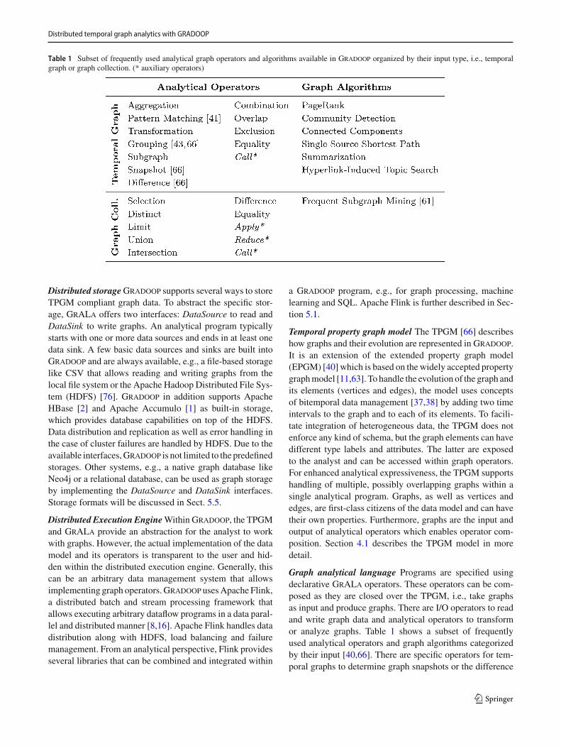
Table 1 Subset of frequently used analytical graph operators and algorithms available in Gradoop organized by their input type, i.e., temporalgraph or graph collection. (* auxiliary operators)
Distributed storageGradoop supports several ways to storeTPGM compliant graph data. To abstract the specific stor-age, GrALa offers two interfaces: DataSource to read andDataSink to write graphs. An analytical program typicallystarts with one or more data sources and ends in at least onedata sink. A few basic data sources and sinks are built intoGradoop and are always available, e.g., a file-based storagelike CSV that allows reading and writing graphs from thelocal file system or the Apache Hadoop Distributed File Sys-tem (HDFS) [76]. Gradoop in addition supports ApacheHBase [2] and Apache Accumulo [1] as built-in storage,which provides database capabilities on top of the HDFS.Data distribution and replication as well as error handling inthe case of cluster failures are handled by HDFS. Due to theavailable interfaces,Gradoop is not limited to the predefinedstorages. Other systems, e.g., a native graph database likeNeo4j or a relational database, can be used as graph storageby implementing the DataSource and DataSink interfaces.Storage formats will be discussed in Sect. 5.5.
Distributed Execution EngineWithinGradoop, the TPGMand GrALa provide an abstraction for the analyst to workwith graphs. However, the actual implementation of the datamodel and its operators is transparent to the user and hid-den within the distributed execution engine. Generally, thiscan be an arbitrary data management system that allowsimplementing graph operators.Gradoop usesApache Flink,a distributed batch and stream processing framework thatallows executing arbitrary dataflow programs in a data paral-lel and distributed manner [8,16]. Apache Flink handles datadistribution along with HDFS, load balancing and failuremanagement. From an analytical perspective, Flink providesseveral libraries that can be combined and integrated within
a Gradoop program, e.g., for graph processing, machinelearning and SQL. Apache Flink is further described in Sec-tion 5.1.
Temporal property graph model The TPGM [66] describeshow graphs and their evolution are represented in Gradoop.It is an extension of the extended property graph model(EPGM) [40] which is based on the widely accepted propertygraphmodel [11,63]. To handle the evolution of the graph andits elements (vertices and edges), the model uses conceptsof bitemporal data management [37,38] by adding two timeintervals to the graph and to each of its elements. To facili-tate integration of heterogeneous data, the TPGM does notenforce any kind of schema, but the graph elements can havedifferent type labels and attributes. The latter are exposedto the analyst and can be accessed within graph operators.For enhanced analytical expressiveness, the TPGM supportshandling of multiple, possibly overlapping graphs within asingle analytical program. Graphs, as well as vertices andedges, are first-class citizens of the data model and can havetheir own properties. Furthermore, graphs are the input andoutput of analytical operators which enables operator com-position. Section 4.1 describes the TPGM model in moredetail.
Graph analytical language Programs are specified usingdeclarative GrALa operators. These operators can be com-posed as they are closed over the TPGM, i.e., take graphsas input and produce graphs. There are I/O operators to readand write graph data and analytical operators to transformor analyze graphs. Table 1 shows a subset of frequentlyused analytical operators and graph algorithms categorizedby their input [40,66]. There are specific operators for tem-poral graphs to determine graph snapshots or the difference
123

C. Rost et al.
between two snapshots as well as temporal versions of moregeneral operators such as pattern matching [41] and graphgrouping [43,66]. Furthermore, there are dedicated trans-formation operators to support data integration [46]. Eachcategory contains auxiliary operators, e.g., to apply unarygraph operators on each graph in a graph collection or to callexternal algorithms. GrALa already integrates well-knowngraph algorithms (e.g., page rank or connected components),which can be seamlessly integrated into a program. Graphoperators will be further described in Sect. 4.2.
Programming interfaces Gradoop provides two options toimplement an analytical program. The most comprehensiveapproach is the Java API containing the TPGM abstractionincluding all operators definedwithinGrALa. Here, the ana-lyst has the highest flexibility of interacting with other Flinkand Java libraries as well as of implementing custom logicfor GrALa operators. For a user-friendly visual definitionof Gradoop programs and a visualization of graph results,we have incorporated Gradoop into the data pipelining toolKNIME Analytics Platform [14]. This extension makes itpossible to use selected GrALa operators within KNIMEanalysis workflows and to execute the resulting workflowson a remote cluster [67,68]. KNIME and the Gradoopextension offer built-in visualization capabilities that can beleveraged for customizable result and graph visualization.
Data integration support Gradoop aims at the analysis ofintegrated data, e.g., knowledge graphs, originating from dif-ferent heterogeneous sources. This can be achieved by firsttranslating the individual sources into a Gradoop represen-tation and then performing data integration for the differentgraphs. Gradoop provides several specific data transforma-tion operators to support this kind of data integration, e.g.,to achieve similarly structured graphs (see Sect. 4.2.6). Fur-thermore, we provide extensive support for entity resolutionand entity clustering within a dedicated framework calledFAMER [70–72] which is based on Gradoop and ApacheFlink. FAMER determines matching entities from two ormore (graph) sources and clusters them together. Such clus-ters of matching entities can then be fused to single entities(with a Fusion operator) for use in an integrated Gradoopgraph. In future work, we will provide a closer integrationof Gradoop and FAMER to achieve a unified data transfor-mation and integration for heterogeneous graph data and theconstruction and evolution of knowledge graphs [59].
4 Temporal property graphmodel
In this section, we present the Temporal Property GraphModel (TPGM) as the graph model of Gradoop that allowsthe representation of evolving graph data and its analysis.Wefirst describe the structural part of TPGM to represent tem-
poral graph data and then discuss the graph operators as partof GrALa. The last subsection briefly discusses the graphalgorithms currently available in Gradoop.
4.1 Graph datamodel
The Property Graph Model (PGM) [11,63] is a widelyaccepted graph data model used by many graph databasesystems [10], e.g., JanusGraph [4], OrientDB [5], Oracle’sGraph Database [22] and Neo4j [57]. A property graph is adirected, labeled and attributed multigraph. Vertex and edgesemantics are expressed using type labels (e.g., Person orknows). Attributes have the form of key-value pairs (e.g.,name:Alice or classYear:2015) and are referred toas properties. Properties are set at the instance level with-out an upfront schema definition. A temporal property graphis a property graph with additional time information onits vertices and edges, which primarily describes the his-torical development of the structure and attributes of thegraph, i.e., when a graph element was available and whenit was superseded. Our presented TPGM adds support fortwo time dimensions, valid and transaction time, to differ-entiate between the evolution of the graph data with respectto the real-world application (valid time) and with respect tothe visibility of changed graph data to the system managingthe data (transaction time). This concept of maintaining twoorthogonal time domains is known as bitemporality [38]. Inaddition, the TPGM supports graph collections, which wereintroduced by the EPGM [40], the non-temporal predecessorof the TPGM. A graph collection contains multiple, possiblyoverlapping property graphs, which are referred to as logi-cal graphs. Like vertices and edges, logical graphs also havebitemporal information, a type label and an arbitrary numberof properties. Before the data model is formally defined, thefollowing preliminaries3 have to be considered:
PreliminariesWe assume two discrete linearly ordered timedomains:Ωval describes the valid-timedomain,whereasΩ t x
describes the transaction-time domain. For each domain, aninstant in time is a time point ωi with limited precision, e.g.,milliseconds. The linear ordering is defined by ωi < ωi+1,which means that ωi happened before ωi+1. A period oftime is defined by a closed-open interval τ = [ωstart , ωend)
that represents a discrete contiguous set of time instances{ω|ω ∈ Ω ∧ ωstart ≤ ω < ωend} starting from ωstart andincluding the start time, continuing toωend but excluding theend time. To separate the time intervals depending on thecorresponding dimension, we use the notion τval and τ t x .
Based on this, a TPGM database is formally defined asfollows:
3 The preliminaries are partly based onmodel definitions of the systemsTGraph [55] and Graphite [27].
123
Distributed temporal graph analytics with GRADOOP
Definition 1 (Temporal Property Graph Modeldatabase) A tuple G = (L, V , E, l, s, t, B, β, K , A, κ)
represents a temporal graph database. L is a finite set oflogical graphs, V is a finite set of vertices and E is a finite setof directed edges with s : E → V and t : E → V assigningsource and target vertex.
Each vertex v ∈ V is a tuple 〈vid, τ val , τ t x 〉, where vid isa unique vertex identifier, τval and τ t x are the time intervalsfor which the vertex is valid with respect to Ωval or Ω t x .Each edge e ∈ E is a tuple 〈eid, τ val , τ t x 〉, where eid is aunique edge identifier that allowsmultiple edges between thesame nodes, τval and τ t x are the time intervals for which theedge exists, analogous to the vertex definition.
B is a set of type labels and β : L ∪ V ∪ E → B assignsa single label to a logical graph, vertex or edge. Similarly,properties are defined as sets of property keys K , propertyvalues A and a partial function κ : (L ∪ V ∪ E) × K⇀A.
A logical graph G ′ = (V ′, E ′, τ val , τ t x ) ∈ L representsa subset of vertices V ′ ⊆ V and a subset of edges E ′ ⊆ E .τval and τ t x are the time intervals for which the logical graphexists in the respective time dimensions. Graph containmentis represented by the mapping l : V ∪ E → P(L) \ {∅}such that ∀v ∈ V ′ : G ′ ∈ l(v) and ∀e ∈ E ′ : s(e), t(e) ∈V ′∧G ′ ∈ l(e). A graph collectionG = {G1,G2, . . . ,Gn} ⊆P(L) is a set of logical graphs.
Constraints Each logical graph has to be a valid directedgraph, implying that for every edge in the graph, theadjacent vertices are also elements in that graph. For-mally: For every logical graph G = (V , E, τ val , τ t x ) andevery edge e = 〈eid, τ val , τ t x 〉 there must exist somev1 = 〈v1id, τ val
1 , τ t x1 〉, v2 = 〈v2id, τ val2 , τ t x2 〉 ∈ V where
s(eid) = v1id and t(eid) = v2id. Additionally, the edgecan only be valid with respect to Ω t x when both verticesare also valid at the same time: τ t x ⊆ τ t x1 ∧ τ t x ⊆ τ t x2 .The same must hold for the valid time domain Ωval : τval ⊆τval1 ∧ τ t x ⊆ τval
2 .Vertices are identified by their unique identifier and their
validity in the transaction-time domain Ω t x , meaning thata temporal graph database may contain two or more ver-tices with the same identifier but different transaction-timevalues. The corresponding intervals of all those verticeshave to be pairwise disjoint, i.e., for every two verticesv1 = 〈v1id, τ val
1 , τ t x1 〉, v2 = 〈v2id, τ val2 , τ t x2 〉 ∈ V it must
hold that v1id = v2id ∧ v1 = v2 �⇒ τ t x1 ∩ τ t x2 = ∅.Edges may be identified in the same way, meaning that thegraph database can also containmultiple edges with the sameidentifier but different transaction time values.
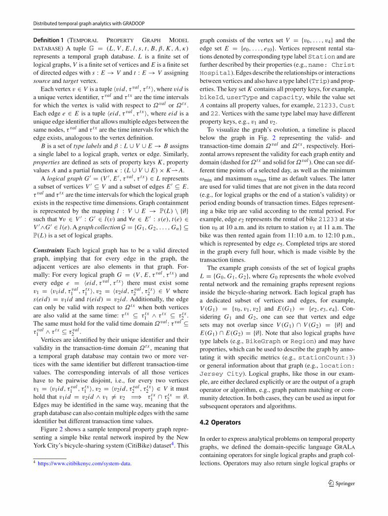
Figure 2 shows a sample temporal property graph repre-senting a simple bike rental network inspired by the NewYork City’s bicycle-sharing system (CitiBike) dataset4. This
4 https://www.citibikenyc.com/system-data.
graph consists of the vertex set V = {v0, . . . , v4} and theedge set E = {e0, . . . , e10}. Vertices represent rental sta-tions denoted by corresponding type label Station and arefurther described by their properties (e.g., name: ChristHospital). Edges describe the relationships or interactionsbetween vertices and also have a type label (Trip) and prop-erties. The key set K contains all property keys, for example,bikeId, userType and capacity, while the value setA contains all property values, for example, 21233, Custand 22. Vertices with the same type label may have differentproperty keys, e.g., v1 and v2.
To visualize the graph’s evolution, a timeline is placedbelow the graph in Fig. 2 representing the valid- andtransaction-time domain Ωval and Ω t x , respectively. Hori-zontal arrows represent the validity for each graph entity anddomain (dashed forΩ t x and solid forΩval ). One can see dif-ferent time points of a selected day, as well as the minimumωmin and maximum ωmax time as default values. The latterare used for valid times that are not given in the data record(e.g., for logical graphs or the end of a station’s validity) orperiod ending bounds of transaction times. Edges represent-ing a bike trip are valid according to the rental period. Forexample, edge e2 represents the rental of bike 21233 at sta-tion v0 at 10 a.m. and its return to station v1 at 11 a.m. Thebike was then rented again from 11:10 a.m. to 12:10 p.m.,which is represented by edge e5. Completed trips are storedin the graph every full hour, which is made visible by thetransaction times.
The example graph consists of the set of logical graphsL = {G0,G1,G2}, where G0 represents the whole evolvedrental network and the remaining graphs represent regionsinside the bicycle-sharing network. Each logical graph hasa dedicated subset of vertices and edges, for example,V (G1) = {v0, v1, v2} and E(G1) = {e2, e3, e4}. Con-sidering G1 and G2, one can see that vertex and edgesets may not overlap since V (G1) ∩ V (G2) = {∅} andE(G1) ∩ E(G2) = {∅}. Note that also logical graphs havetype labels (e.g., BikeGraph or Region) and may haveproperties, which can be used to describe the graph by anno-tating it with specific metrics (e.g., stationCount:3)or general information about that graph (e.g., location:Jersey City). Logical graphs, like those in our exam-ple, are either declared explicitly or are the output of a graphoperator or algorithm, e.g., graph pattern matching or com-munity detection. In both cases, they can be used as input forsubsequent operators and algorithms.
4.2 Operators
In order to express analytical problems on temporal propertygraphs, we defined the domain-specific language GrALacontaining operators for single logical graphs and graph col-lections. Operators may also return single logical graphs or
123

C. Rost et al.
Fig. 2 Example temporal property graph of a bike rental network with two non-overlapping logical graphs
graph collections (i.e., they are closed over the data model),thereby enabling operator composition. In the following, weuse the terms collection and graph collection as well asgraph and logical graph interchangeably. Table 2 lists ourgraph operators including their corresponding pseudocodesyntax for calling them inGrALa. The syntax adopts the con-cept of higher-order functions for several operators (e.g., touse aggregate or predicate functions as operator arguments).Based on the input of operators, we distinguish betweengraph operators and collection operators as well as unaryand binary operators (single graph/collection vs. two graph-s/collections as input). There are also auxiliary operators toapply graph operators on collections or to call specific graph
algorithms. In addition to the listed ones, we provide opera-tors to import external datasets to Gradoop by mapping thedata to the TPGM data model, i.e., creating graphs, verticesand edges including respective labels, properties and bitem-poral attributes. In the following, we focus on a subset of theoperators and refer to our publications [40,41,43,65,66] andGradoop’s GitHub–Wiki [64] for detailed explanations.
4.2.1 Subgraph
In temporal and heterogeneous graphs, often only a spe-cific subgraph is of interest for analytics, e.g., only personsand their relationships in a social network. The subgraph
123

Distributed temporal graph analytics with GRADOOP
Table 2 TPGM graph operators specified with GrALa
operator is used to extract the graph of interest by applyingpredicate functions on each element of the vertex and edgesets of the input graph. Within a predicate function, the userhas access to label, properties and bitemporal attributes ofthe specific entity and can express arbitrary logic. Formally,given a logical graph G(V , E) and the predicate functionsϕv : V → {true, f alse} and ϕe : E → {true, f alse},the subgraph operator returns a new graph G ′ ⊆ G withV ′ = {v | v ∈ V ∧ ϕv(v)} and E ′ = {〈vi , v j 〉 | 〈vi , v j 〉 ∈E ∧ ϕe(〈vi , v j 〉) ∧ vi , v j ∈ V ′}. In the following exam-
ple, we extract the subgraph containing all vertices labeledStation having a property capacity with a value lessthan 30 and their edges of type Trip with a propertygender which value is equal to female:5
subgraph = g0.subgraph((v => v.label == ’Station ’ AND
v.capacity < 30),
5 In our listings, label and property values of an entity n are beingaccessed using dot notation, e.g., n.label or n.name.
123

C. Rost et al.
(e => e.label == ’Trip ’ ANDe.gender == ’female ’))
Applied to the graph G0 of Fig. 2, the operator returnsa new logical graph described through G ′ = 〈{v2, v3, v4},{e8, e9}〉. By omitting either a vertex or an edge predicatefunction exclusively, the operator is also suitable to declarevertex-induced or edge-induced subgraphs, respectively.
4.2.2 Snapshot
The snapshot operator is used to retrieve a valid snapshot ofthe whole temporal graph either at a specific point in timeor a subgraph that is valid during a given time range. It isformally equal to the subgraph operator, but allows for theapplication of specific time-dependent predicate functions,which were partly adapted from SQL:2011 [47] and Allen’sinterval algebra [9].
The predicate asOf (t) returns the graph at a specificpoint in time, whereas all others, like fromTo(t1, t2), pre-cedes(t1, t2) or overlaps(t1, t2), return a graph with allchanges in the specified interval. For each predicate func-tion, the valid-time domain is used by default but can bespecified through an additional argument. Note that a TPGMgraph may represent the entire history of all graph changes.For analysis of the current graph state, it is therefore advis-able to use the snapshot operator with the asOf() predicate,parameterized with the current system timestamp. Bitempo-ral predicates can be defined through multiple operator calls.For example, the following GrALa operator call retrieves asnapshot of the graph for valid time 2020-09-06 at 9 a.m. andat the current system time as the transaction time:
pastGraph = g0.snapshot(
asOf(CURRENT_TIMESTAMP()),TRANSACTION_TIME)
.snapshot(asOf ( ’2019-09-06 09:00:00 ’) ,VALID_TIME)
In the timeline of Fig. 2, one can see that edges e1, e6, e8as well as all vertices and graphs meet the valid-time con-dition and are therefore part of the resulting graph. Allvisible elements exist at the current system time accord-ing to the transaction-time domain; therefore, the resultdoes not change. However, if one changes the argumentof the first (transaction time) predicate to ’2019-09-0609:55:00’, edges e6 and e8 would no longer belong to theresult set, since the information about these trips was not yetpersisted at this point in time.
4.2.3 Difference
In temporal graphs, the difference of two temporal snapshotsmay be of interest for analytics to investigate how a graph haschanged over time. To represent these changes, a differencegraph can be usedwhich is the union of both snapshots and inwhich each graph element is annotated as an added, deletedor persistent element.
The difference operator of GrALa consumes two graphsnapshots defined by temporal predicate functions and cal-culates the difference graph as a new logical graph. Theannotations are stored as a property _diff on each graphelement, whereas the value of the property will be a numberindicating that an element is either equal in both snapshots(0) or added (1) or removed (-1) in the second snapshot. Thisresulting graph can then be used by subsequent operators to,for example, filter for added elements, group removed ele-ments or aggregate specific values of persistent elements. Forthe given example in Fig. 2, the following operator call cal-culates the difference between the graph at 9 a.m. and 10 a.m.of the given day:
diffGraph = g0.diff(asOf ( ’2019-09-06 09:00:00 ’) ,asOf ( ’2019-09-06 10:00:00 ’) ,VALID_TIME)
The operator returns a new logical graph describedthrough G ′ where V (G ′) = {v0, . . . , v4} and E(G ′) ={e1, e2, e6, e7, e8}. Further, the property key _diff is addedto K and the values {−1, 0, 1} are added to A. Since all ver-tices and the edge e8 are valid in both snapshots, a property_diff:0 is added to them. The edges e6 and e1 are nolonger available in the second snapshot; therefore, they areextended by the property _diff:-1, whereas the edges e2and e7 are annotated by _diff:1 to show that they werecreated during this time period.
4.2.4 Time-dependent Graph Grouping
For large graphs, it is often desirable to structurally groupvertices and edges into a condensedgraphwhichhelps uncov-ering insights about hidden patterns [40,43] and exploratoryanalyze an evolving graph at different levels of temporal andstructural granularity. Let G ′ be the condensed graph of G,then each vertex in V ′ represents a group of vertices in Vand edges in E ′ represent a group of edges between the ver-tex group members in V . Formally, V ′ = {v′
1, v′2, . . . , v
′k}
where v′i is called a supervertex and ∀v ∈ V , sν(v) is the
supervertex of v.
123

Distributed temporal graph analytics with GRADOOP
Vertices are grouped together based on the values returnedby key functions. A key function k : V → V is a functionmapping eachvertex to a value in some setV . Let {k1, . . . , kn}be a set of vertex grouping key functions, then ∀u, v ∈V : sν(u) = sν(v) ⇐⇒ ∧n
i=1 ki (u) = ki (v). Somekey functions are provided by the system, namely label()= v �→ β(v) mapping vertices to their label, property(key)= v �→ κ(v, key) mapping vertices to the according prop-erty value as well as timeStamp(...) and duration(...) usedto extract temporal data from elements. The latter functionscan be used to extract either the start or end time of both timedomains or their duration. It is also possible to retrieve date–time fields from timestamps, like the corresponding day ofthe week or the month. This can be used, for example, togroup edges that became valid in the same month together.Further, user defined key functions are supported by the oper-ator, e.g., to calculate a spatial index in form of a grid cellidentifier from latitude and longitude properties to group allvertices of that virtual grid cell together. The values returnedby the key functions are being stored on the supervertex asnew properties.
Similarly, E ′ = {e′1, e
′2, . . . , e
′l} where e′
i is called asuperedge and sε(u, v) is the superedge for 〈u, v〉. Edgegroups are determined along the supervertices and a set ofedge keys {k1, . . . , km}, where k j : E → V are grouping keyfunctions analogous to the vertex keys, such that ∀e, f ∈E : sε(s(e), t(e)) = sε(s( f ), t( f )) ⇐⇒ sν(s(e)) =sν(s( f )) ∧ sν(t(e)) = sν(t( f )) ∧ ∧m
j=1 k j (e) = k j ( f ). Thesame key functions mentioned above for vertices are alsoapplicable for edges. Additionally, vertex and edge aggre-gate functions γv : P(V) → A and γe : P(E) → A are usedto compute aggregated property values for grouped verticesand edges, e.g., the average duration of rentals in a group orthe number of group members. The aggregate value is storedas new property at the supervertex and superedge, respec-tively. The following example shows the application of thegrouping operator using GrALa:
1 summary = g0.groupBy(2 [label(), property(’regionId ’)],3 (superVertex , vertices =>4 superVertex[’count ’]5 = vertices.count(),6 superVertex[’lat ’]7 = avg(vertices.lat),8 superVertex[’lon ’]9 = avg(vertices.lon)),
10 [label(), timeStamp(11 VALID_TIME , FROM , HOUR_OF_DAY)],12 (superEdge , edges =>13 superEdge[’count ’] = edges.count(),14 superEdge[’avgTripLen ’] =15 averageDuration(VALID_TIME ))
The goal of this example is to group Stations and Tripsin the graph of Fig. 2 by region and to calculate the numberof stations and the average coordinates of stations in each
region. Furthermore, we group trip edges by the hour of theday in which the trip was started and calculate the numberand average duration of trips. For example, we can gain aninsight into how popular each region was and which routebetween which regions was the most popular or took thelongest all day. In line 2, we define the vertex grouping keys.Here, we want to group vertices by type label (using thelabel() key function) and property keyregionId (usingthe property() key function). Edges are grouped by labeland by the start of the valid time interval. The timeStampkey function was used for the latter to extract the start of thevalid time interval and to calculate the hour of the day for thistime (lines 10–11). Type labels are added as grouping keys inboth cases, since we want to retain this information on super-vertices and superedges. In lines 3–9 and 12–15, we declarethe vertex and edge aggregate functions, respectively. Bothreceive a superelement (i.e.,superVertex,superEdge)and a set of group members (i.e., vertices, edges) asinputs. They then calculate values for the group and attachthem as properties to the superelement. In our example, acount property is set storing the number of elements in thegroup. We also use the avg function to calculate the averagevalue of a numeric property and the averageDurationfunction to get the average length of the valid time intervalfor elements. Figure. 3 shows the resulting logical graph forthis example.
4.2.5 Temporal pattern matching
A fundamental operation of graph analytics is the retrievalof subgraphs isomorphic or homomorphic6 to a user-definedpattern graph. An important requirement in the scope oftemporal graphs is the access and usage of the temporalinformation, i.e., time intervals and their bounds, inside thepattern. For example, given a bike-sharing network, an ana-lyst may be interested in a chronological sequence of tripsof the same bike that started at a particular station witha radius of three hops (stations). To support such queries,GrALa provides the pattern matching operator [41], wherethe operator argument is a pattern (query) graph Q includ-ing predicates for its vertices and edges. To describe suchquery graphs, we defined TemporalGDL7, a query languagewhich is based on the core concepts of Cypher8, especially its“MATCH” and “WHERE” clauses. For example, the expres-sion (a)-[e]->(b) denotes a directed edge e from vertexa to vertex b and can be used in a MATCH clause. Predi-cates are either embedded into the pattern by defining type
6 GrALa support different morphism semantics, see [41].7 TemporalGDL is an extension of the Graph Definition Language(GDL)which is open source available at https://github.com/dbs-leipzig/gdl.8 http://www.opencypher.org/.
123

C. Rost et al.
Fig. 3 Result graph of grouping example
labels and properties or expressed in the WHERE clause.For a more detailed description of the (non-temporal) lan-guage on which TemporalGDL is based, we refer to ourprevious publication [41]. We extended the language by var-ious syntactic constructs that are partly inspired by Allen’sconventions [9] and the SQL:2011 standard [47], to supportthe TPGM-specific bitemporal attributes. These extensionsenable the construction of time-dependent patterns, e.g., todefine a chronological order of elements or to define Booleanrelations by accessing the element’s temporal intervals andtheir bounds. Table 3 gives an overview of a subset of theTemporalGDL syntax including access options for inter-vals and their bounds of both dimensions (e.g., a.valto get the valid time interval of the graph element that isrepresented by variable a), a set of binary relations for inter-vals and timestamps (e.g., a.val.overlaps(b.val) tocheck whether the valid time intervals of the graph elementsassigned to a and b overlap), functions to create a durationtime constant of a specific time unit (e.g., Seconds(10)to get a duration constant of 10 seconds) and binary rela-tions between duration constants and interval durations, e.g,a.val.shorterThan(b.val) to check whether theduration of the valid time interval of a is shorter than the oneof b or a.val.longerThan(Minutes(5)) to checkwhether the duration of the interval is longer than five min-utes.
Pattern matching is applied to a graph G and returns agraph collection G′, such thatG ′ ∈ G′ ⇔ G ′ ⊆ G∧G ′ � Q,i.e., G′ contains all isomorphic (or homomorphic) subgraphsof G that match the pattern. The pattern matching operatoris applied on a logical graph as follows:
matches = g0.query("MATCH (a:Station {name:’Christ Hospital ’})
-[e:Trip]->(b:Station)(b:Station)-[f:Trip]->(c:Station)(c:Station)-[g:Trip]->(d:Station)
WHERE e.bikeId = f.bikeId ANDf.bikeId = g.bikeId ANDe.val.precedes(f.val) ANDg.val.succeeds(f.val)")
Table 3 Overview of TemporalGDL’s syntax to support temporal graphpatterns
The shown TemporalGDL pattern graph reflects theaforementioned bike-sharing network query. In the exam-ple, we describe a pattern of four vertices and threeedges, which are assigned to variables (a,b,c,d for ver-tices and e,f,g for edges). Variables are optionally fol-lowed by a label (e.g., a:Station) and properties (e.g.,{name:’Christ Hospital’}). More complex predi-cates can be expressed within the WHERE clause. Here, theuser has access to vertex and edge properties using their vari-able and property keys (e.g., e.bikeId = f.bikeId).In addition, bitemporal information of the elements canbe accessed in a similar way using predefined identifiers(e.g., e.val) as described before. A chronological orderof the edges is defined by binary relations, for example,e.val.precedes(f.val). When called for graph G0
123
Distributed temporal graph analytics with GRADOOP
Stationname: 10 Ave & W 28 Stcapacity: 49 lat: 40.75066386lon: -74.00176802regionId: 71
TripbikeId: 21233userType: Subgender: maleyob: 1971
Station 1name: E 17 St & Broadwaycapacity: 66 lat: 40.73704984lon: -73.99009296regionId: 71
Station 4name: Christ Hospitalcapacity: 22 lat: 40.734785818lon: -74.050443636regionId: 70
Stationname: Essex Light Railcapacity: 22 lat: 40.7127742lon: -74.0364857regionId: 70
mapping: { a : 4, b : 0, c : 1, d : 3, e : 1, f : 2, g :5}
1
TripbikeId: 21233userType: Subgender: femaleyob: 1980
TripbikeId: 21233userType: Custgender: maleyob: 1981
4
2
5
0
3
Fig. 4 Result graph of temporal pattern matching example
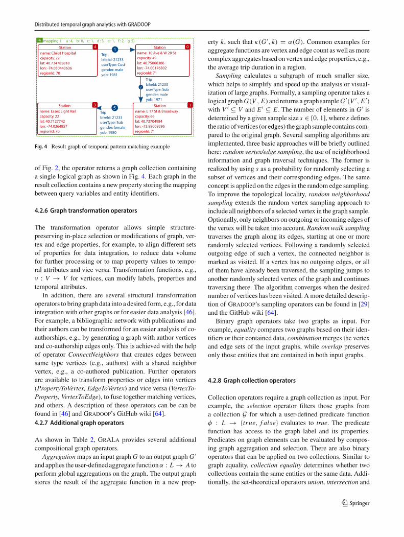
of Fig. 2, the operator returns a graph collection containinga single logical graph as shown in Fig. 4. Each graph in theresult collection contains a new property storing themappingbetween query variables and entity identifiers.
4.2.6 Graph transformation operators
The transformation operator allows simple structure-preserving in-place selection or modifications of graph, ver-tex and edge properties, for example, to align different setsof properties for data integration, to reduce data volumefor further processing or to map property values to tempo-ral attributes and vice versa. Transformation functions, e.g.,ν : V → V for vertices, can modify labels, properties andtemporal attributes.
In addition, there are several structural transformationoperators to bring graph data into a desired form, e.g., for dataintegration with other graphs or for easier data analysis [46].For example, a bibliographic network with publications andtheir authors can be transformed for an easier analysis of co-authorships, e.g., by generating a graph with author verticesand co-authorship edges only. This is achieved with the helpof operator ConnectNeighbors that creates edges betweensame type vertices (e.g., authors) with a shared neighborvertex, e.g., a co-authored publication. Further operatorsare available to transform properties or edges into vertices(PropertyToVertex, EdgeToVertex) and vice versa (VertexTo-Property, VertexToEdge), to fuse together matching vertices,and others. A description of these operators can be can befound in [46] and Gradoop’s GitHub wiki [64].4.2.7 Additional graph operators
As shown in Table 2, GrALa provides several additionalcompositional graph operators.
Aggregationmaps an input graph G to an output graph G ′and applies the user-defined aggregate functionα : L → A toperform global aggregations on the graph. The output graphstores the result of the aggregate function in a new prop-
erty k, such that κ(G ′, k) = α(G). Common examples foraggregate functions are vertex and edge count aswell asmorecomplex aggregates based onvertex and edge properties, e.g.,the average trip duration in a region.
Sampling calculates a subgraph of much smaller size,which helps to simplify and speed up the analysis or visual-ization of large graphs. Formally, a sampling operator takes alogical graphG(V , E) and returns a graph sampleG ′(V ′, E ′)with V ′ ⊆ V and E ′ ⊆ E . The number of elements in G ′ isdetermined by a given sample size s ∈ [0, 1], where s definesthe ratio of vertices (or edges) the graph sample contains com-pared to the original graph. Several sampling algorithms areimplemented, three basic approaches will be briefly outlinedhere: random vertex/edge sampling, the use of neighborhoodinformation and graph traversal techniques. The former isrealized by using s as a probability for randomly selecting asubset of vertices and their corresponding edges. The sameconcept is applied on the edges in the random edge sampling.To improve the topological locality, random neighborhoodsampling extends the random vertex sampling approach toinclude all neighbors of a selected vertex in the graph sample.Optionally, only neighbors on outgoing or incoming edges ofthe vertex will be taken into account. Random walk samplingtraverses the graph along its edges, starting at one or morerandomly selected vertices. Following a randomly selectedoutgoing edge of such a vertex, the connected neighbor ismarked as visited. If a vertex has no outgoing edges, or allof them have already been traversed, the sampling jumps toanother randomly selected vertex of the graph and continuestraversing there. The algorithm converges when the desirednumber of vertices has been visited. Amore detailed descrip-tion of Gradoop’s sampling operators can be found in [29]and the GitHub wiki [64].
Binary graph operators take two graphs as input. Forexample, equality compares two graphs based on their iden-tifiers or their contained data, combinationmerges the vertexand edge sets of the input graphs, while overlap preservesonly those entities that are contained in both input graphs.
4.2.8 Graph collection operators
Collection operators require a graph collection as input. Forexample, the selection operator filters those graphs froma collection G for which a user-defined predicate functionφ : L → {true, f alse} evaluates to true. The predicatefunction has access to the graph label and its properties.Predicates on graph elements can be evaluated by compos-ing graph aggregation and selection. There are also binaryoperators that can be applied on two collections. Similar tograph equality, collection equality determines whether twocollections contain the same entities or the same data. Addi-tionally, the set-theoretical operators union, intersection and
123
C. Rost et al.
difference compute new collections based on graph identi-fiers.
It is often necessary to execute a unary graph operator onmore than one graph, for example, to perform aggregation forall graphs in a collection. Not only the previously introducedoperators subgraph, matching and grouping, but all otheroperators with single logical graphs as in- and output (i.e.,op : L → L) can be executed on each element of a graph col-lection using the apply operator. Similarly, in order to applya binary operator on a graph collection, GrALa adopts thereduce operator as often found in functional programminglanguages. The operator takes a graph collection and a com-mutative binary graph operator (i.e., op : L × L → L) asinput and folds the collection into a single graph by recur-sively applying the operator.
4.3 Iterative graph algorithms
In addition to the presented graph and collection opera-tors, advanced graph analytics often requires the use ofapplication-specific graph algorithms. One application is theextraction of subgraphs that cannot be achieved by patternmatching, e.g., the detection of communities [48] and theirevolution [30].
To support external algorithms, GrALa provides genericcall operators (see Table 2), which may have graphs andgraph collections as input or output. Depending on the out-put type,we distinguish between so-calledcallForGraphand callForCollection operators. Using the formerfunction, a user has access to the API and complete library ofiterative graph algorithms of Apache Flink’s Gelly [3], whichis the Apache Flink implementation of Google Pregel [52].By utilizing Flink’s dataset iteration, co-group and flatMapfunctions Gelly is able to provide different kinds of iterativegraph algorithms. For now, vertex iteration, gather–sum–apply and scatter–gather algorithms are supported. However,since Gelly is based on the property graph model we use abidirectional translation between Gradoop’s logical graphand Gelly’s property graph, as described in Sect. 5.4. Thus,Gradoop already provides a set of algorithms that can beseamlessly integrated into a graph analytical program (seeTable 1), e.g., PageRank, Label Propagation and ConnectedComponents. Besides, we provide TPGM-tailored algorithmimplementations, e.g., for frequent subgraph mining (FSM)within a graph collection [61].
5 Implementation
In this chapter, we will describe the implementation of theTPGM and GrALa on top of a distributed system. SinceGradoop programs model a dataflow where one or multi-ple temporal graphs are sequentially processed by chaining
graph operators, the utilization of distributed dataflow sys-tems such as Apache Spark [84] and Apache Flink [16]is especially promising. These systems offer, in contrast toMapReduce [24], a wider range of dataflow operators and theability to keep data in main memory between the executionof those operators. The major challenges of implementinggraph operators in these systems are identifying an appropri-ate graph representation and an efficient combination of theprimitive dataflow operators to express graph operator logic.
As discussed in Sect. 2, the most recent approaches tolarge-scale graph analytics are libraries on top of such dis-tributed dataflow frameworks, e.g., GraphX [83] on ApacheSpark or Gelly [3] on Apache Flink. These libraries arewell suited for executing iterative algorithms on distributedgraphs in combinationwith general data transformation oper-ators provided by the underlying frameworks. However, theimplemented graph data models have no support for tempo-ral graphs, collections and are generic, whichmeans arbitraryuser-defined data can be attached to vertices and edges. Inconsequence, model-specific operators, i.e., such based onlabels, properties or the time attributes, need to be user-defined, too. Hence, using those libraries to solve complexanalytical problems becomes a laborious programming task.
We thus implemented Gradoop on top of Apache Flinkto provide new features for flexible and general-purposegraph analytics and to benefit from existing capabilities tolarge-scale data and graph processing at the same time. Themajority of graph algorithms listed in Table 1 are available inFlink Gelly. Gradoop adds automatic transformation fromTPGM graphs into Gelly graphs and vice versa, as laterdescribed. In this section, we will briefly introduce Flinkand its programming concepts. We will further show howthe TPGM graph representation and a subset of the intro-duced operators, including graph algorithms, are mapped tothose concepts. The last section focuses on persistent graphformats.
5.1 Apache Flink
Apache Flink [8,16] supports the declarative definition andexecution of distributed dataflow programs sourced fromstreaming and batch data. The basic abstractions of such pro-grams are DataSets (or DataStreams) and Transformations.A Flink DataSet is an immutable, distributed collection ofarbitrary data objects, e.g., Java POJOs or tuple types, andtransformations are higher-order functions that describe theconstruction of new DataSets either from existing ones orfrom data sources. Application logic is encapsulated in user-defined functions (UDFs), which are provided as argumentsto the transformations and applied toDataSet elements.Well-known transformations are map and reduce, additional onesare adapted from relational algebra, e.g., projection, selec-tion, join and grouping (see Sect. 4.2). To describe a dataflow,
123
Distributed temporal graph analytics with GRADOOP
a program may include multiple chained transformations.During executionFlink handles programoptimization aswellas data distribution and parallel processing across a clusterof machines.
The fundamental approach of sequentially applying trans-formations on distributed datasets is inherited by Gradoop:Instead of generic DataSets, the user applies transformations(i.e., graph operators and algorithms) to graphs and collec-tions of those. Transformations create new graphs which inturn can be used as input for subsequent operators herebyenabling arbitrary complex graph dataflows. Gradoop canbe used standalone or in combination with any other libraryavailable in the Flink ecosystem, e.g., for machine learn-ing (Flink ML), graph processing (Gelly) or SQL (FlinkTable).
5.2 Graph representation
One challenge of implementing a system for static and tem-poral graph analytics on a dataflow system is the design ofa graph representation. Such a representation is requiredto support all data model features (i.e., support differententities, labels, properties and bitemporal intervals) andalso needs to provide reasonable performance for all graphoperators.
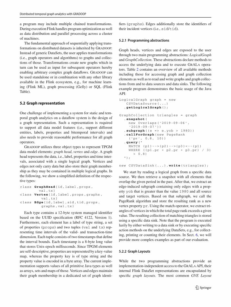
Gradoop utilizes three object types to represent TPGMdata model elements: graph head, vertex and edge. A graphhead represents the data, i.e., label, properties and time inter-vals, associated with a single logical graph. Vertices andedges not only carry data but also store their graph member-ship as they may be contained in multiple logical graphs. Inthe following, we show a simplified definition of the respec-tive types:
class GraphHead{id ,label ,props ,val ,tx}
class Vertex{id ,label ,props ,graphs ,val ,tx}
class Edge{id ,label ,sid ,tid ,props ,graphs ,val ,tx}
Each type contains a 12-byte system managed identifierbased on the UUID specification (RFC 4122, Version 1).Furthermore, each element has a label of type string, a setof properties (props) and two tuples (val and tx) rep-resenting time intervals of the valid- and transaction-timedimension. Each tuple consists of two timestamps that definethe interval bounds. Each timestamp is a 8-byte long valuethat stores Unix-epoch milliseconds. Since TPGM elementsare self-descriptive, properties are represented by a key-valuemap, whereas the property key is of type string and theproperty value is encoded in a byte array. The current imple-mentation supports values of all primitive Java types as wellas arrays, sets andmaps of those. Vertices and edgesmaintaintheir graph membership in a dedicated set of graph identi-
fiers (graphs). Edges additionally store the identifiers oftheir incident vertices (i.e., sid/tid).
5.2.1 Programming abstractions
Graph heads, vertices and edges are exposed to the userthrough two main programming abstractions: LogicalGraphandGraphCollection. These abstractions declare methods toaccess the underlying data and to execute GrALa opera-tors. Table 2 contains an overview of all available methodsincluding those for accessing graph and graph collectionelements as well as to read andwrite graphs and graph collec-tions from and to data sources and data sinks. The followingexample program demonstrates the basic usage of the JavaAPI:
LogicalGraph graph = newCSVDataSource (...)
.getLogicalGraph ();
GraphCollection triangles = graph.snapshot(
new Overlaps (’2019-09-06’,’2019-09-07’))
.subgraph ((e => e.yob > 1980))
.callForGraph(new PageRank(’pr ’, 0.8, 10))
.query("MATCH (p1)-->(p2)-->(p3)<--(p1)WHERE ((p1.pr + p2.pr + p3.pr) / 3)
> 0.8)");
new CSVDataSink (...). write(triangles );
We start by reading a logical graph from a specific datasource. We then retrieve a snapshot with all elements thatoverlap the given period in the past. After that, we extract anedge-induced subgraph containing only edges with a prop-erty yob that is greater than the value 1980 and all sourceand target vertices. Based on that subgraph, we call thePageRank algorithm and store the resulting rank as a newvertex property pr. Using the match operator, we extract tri-angles of vertices inwhich the total page rank exceeds a givenvalue. The resulting collection ofmatching triangles is storedusing a specific data sink. Note that the program is executedlazily by either writing to a data sink or by executing specificaction methods on the underlying DataSets, e.g., for collect-ing, printing or counting their elements. In Sect. 6, we willprovide more complex examples as part of our evaluation.
5.2.2 Graph Layouts
While the two programming abstractions provide animplementation-independent access to theGrALaAPI, theirinternal Flink DataSet representations are encapsulated byspecific graph layouts. The most common GVE Layout
123

C. Rost et al.
Fig. 5 GVE layout of Gradoop. The accuracy of the timestamps has been reduced for readability reasons
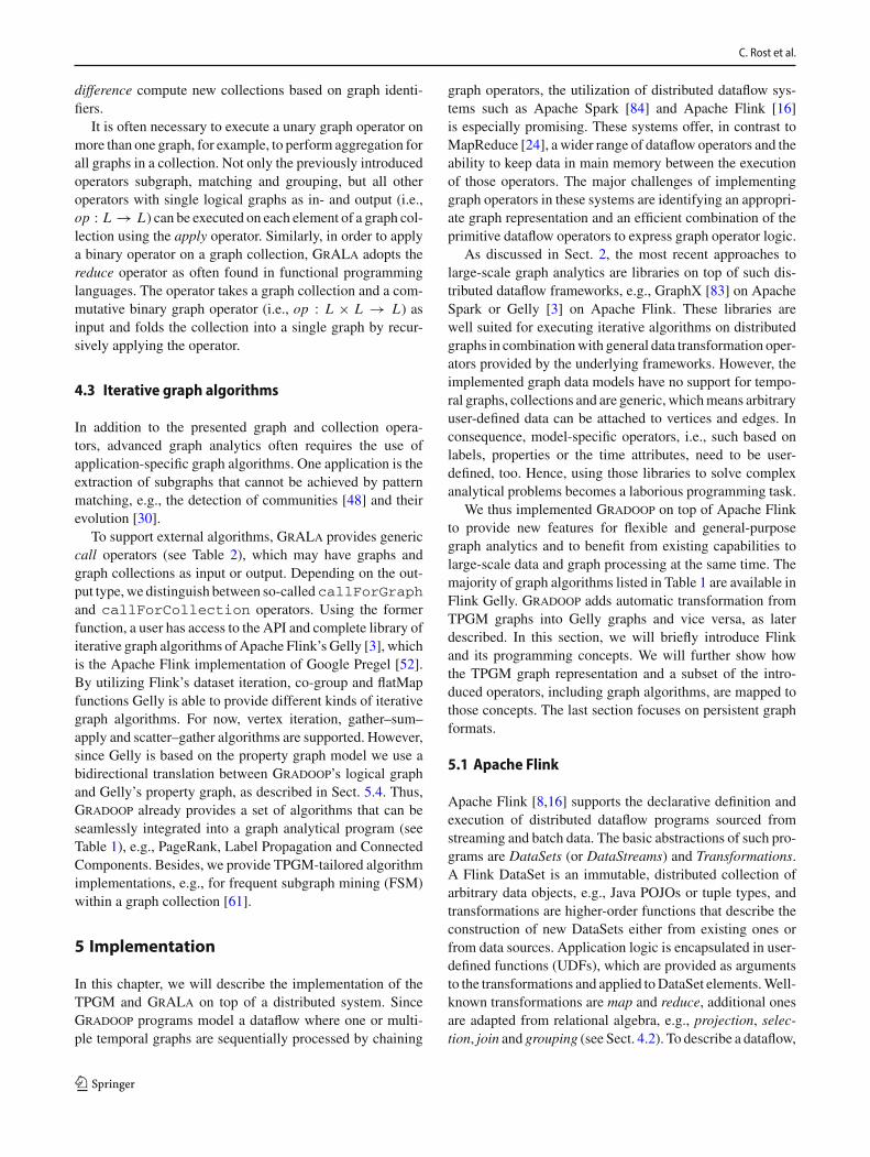
(Graph-Vertex-Edge layout) is the default for single logi-cal graphs and graph collections. The layout corresponds toa relational view of a graph collection by managing a dedi-cated Flink DataSet for each TPGM element type and usingentity identifiers as primary and foreign keys. Operationsthat combine data, e.g., computing the outgoing edges foreach vertex, require join operations between the respectiveDataSets. Since graph containment information is embeddedinto vertex and edge entities, an additional DataSet storingmapping information is not required. Another experimentallayout is IndexedGVE, a variation of theGVE layout inwhichvertex and edge data are partitioned into separate DataSetsbased on the entity label. Other user-defined graph layoutscan be easily integrated by implementing against a providedinterface.
Figure 5 shows an example instance of the GVE layoutfor a graph collection containing logical graphs of Fig. 2.The first DataSet L stores the data attached to logical graphs,vertex data is stored in a second DataSet V and edge data ina third, E . Vertices and edges store a set of graph identifierswhich is a superset of the graph identifiers in L as an entity canbe contained in additional logical graphs (e.g.,G0 andG1). Alogical graph is a special case of a graph collection in whichthe L DataSet contains a single element. Each element storesin addition the two time intervals to capture the visibility forthe valid- and transaction-time dimension.
5.3 Graph operators
The second challenge that needs to be solved when imple-menting a graph framework on a dataflow system is theefficient mapping of graph operators to transformations pro-vided by the underlying system. Table 4 introduces a subset
of transformations available in Apache Flink. Well-knowntransformations have been adopted from the MapReduceparadigm [24]. For example, the map transformation isapplied on a DataSet of elements of type IN and producesa DataSet containing elements of type OUT. Application-specific logic is expressed through a user-defined function(udf: IN -> OUT) that maps an element of the inputDataSet to exactly one element of the output DataSet. Fur-ther DataSet transformations are well known from relationalsystems, e.g., select (filter), join, group-by, project and dis-tinct.
Subsequently, we will explain the mapping of graph oper-ators to Flink transformations.Wewill focus on the operatorsintroduced in Sect. 4: subgraph, snapshot, difference, time-dependent grouping and temporal pattern matching. For alloperators we assume the input graph to be represented in theGVE layout (see Sect. 5.2.2).
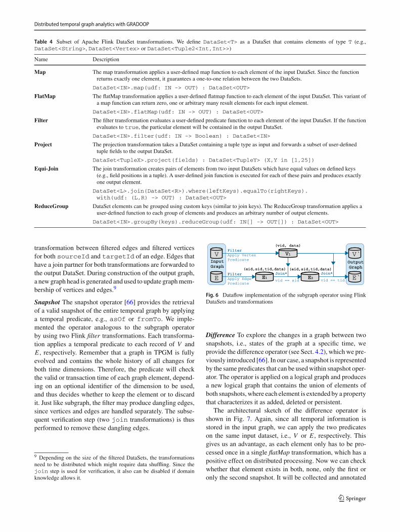
Subgraph The subgraph operator takes a logical graph andtwo user-defined predicate functions (one for vertices, onefor edges) as input. The result is a new logical graph contain-ing only those vertices and edges that fulfill the predicates.Figure 6 illustrates the corresponding dataflow program. Thedataflow is organized from left to right, starting from the ver-tex and edge DataSets of the input graph. Descriptions onthe arrows highlight the applied Flink transformation and itssemantics in the operator context. First,weuse thefilter trans-formation to apply the user-defined predicate functions on thevertex and edge DataSets (e.g., (v => v.capacity >=40)). The resulting vertex DataSet V1 can already be usedto construct the output graph. However, we have to ensurethat no dangling edges exist, i.e., only those filtered edges areselected where source and target vertex are contained in theoutput vertex set. To achieve that, the operator performs a join
123
Distributed temporal graph analytics with GRADOOP
Table 4 Subset of Apache Flink DataSet transformations. We define DataSet<T> as a DataSet that contains elements of type T (e.g.,DataSet<String>, DataSet<Vertex> or DataSet<Tuple2<Int,Int>>)
Name Description
Map The map transformation applies a user-defined map function to each element of the input DataSet. Since the functionreturns exactly one element, it guarantees a one-to-one relation between the two DataSets.
DataSet<IN>.map(udf: IN -> OUT) : DataSet<OUT>
FlatMap The flatMap transformation applies a user-defined flatmap function to each element of the input DataSet. This variant ofa map function can return zero, one or arbitrary many result elements for each input element.
DataSet<IN>.flatMap(udf: IN -> OUT) : DataSet<OUT>
Filter The filter transformation evaluates a user-defined predicate function to each element of the input DataSet. If the functionevaluates to true, the particular element will be contained in the output DataSet.
DataSet<IN>.filter(udf: IN -> Boolean) : DataSet<IN>
Project The projection transformation takes a DataSet containing a tuple type as input and forwards a subset of user-definedtuple fields to the output DataSet.
DataSet<TupleX>.project(fields) : DataSet<TupleY> (X,Y in [1,25])
Equi-Join The join transformation creates pairs of elements from two input DataSets which have equal values on defined keys(e.g., field positions in a tuple). A user-defined join function is executed for each of these pairs and produces exactlyone output element.
DataSet<L>.join(DataSet<R>).where(leftKeys).equalTo(rightKeys).with(udf: (L,R) -> OUT) : DataSet<OUT>
ReduceGroup DataSet elements can be grouped using custom keys (similar to join keys). The ReduceGroup transformation applies auser-defined function to each group of elements and produces an arbitrary number of output elements.
DataSet<IN>.groupBy(keys).reduceGroup(udf: IN[] -> OUT[]) : DataSet<OUT>
transformation between filtered edges and filtered verticesfor both sourceId and targetId of an edge. Edges thathave a join partner for both transformations are forwarded tothe output DataSet. During construction of the output graph,a newgraph head is generated and used to update graphmem-bership of vertices and edges.9
Snapshot The snapshot operator [66] provides the retrievalof a valid snapshot of the entire temporal graph by applyinga temporal predicate, e.g., asOf or fromTo. We imple-mented the operator analogous to the subgraph operatorby using two Flink filter transformations. Each transforma-tion applies a temporal predicate to each record of V andE , respectively. Remember that a graph in TPGM is fullyevolved and contains the whole history of all changes forboth time dimensions. Therefore, the predicate will checkthe valid or transaction time of each graph element, depend-ing on an optional identifier of the dimension to be used,and thus decides whether to keep the element or to discardit. Just like subgraph, the filter may produce dangling edges,since vertices and edges are handled separately. The subse-quent verification step (two join transformations) is thusperformed to remove these dangling edges.
9 Depending on the size of the filtered DataSets, the transformationsneed to be distributed which might require data shuffling. Since thejoin step is used for verification, it also can be disabled if domainknowledge allows it.
Fig. 6 Dataflow implementation of the subgraph operator using FlinkDataSets and transformations
Difference To explore the changes in a graph between twosnapshots, i.e., states of the graph at a specific time, weprovide the difference operator (see Sect. 4.2), which we pre-viously introduced [66]. In our case, a snapshot is representedby the same predicates that can be usedwithin snapshot oper-ator. The operator is applied on a logical graph and producesa new logical graph that contains the union of elements ofboth snapshots, where each element is extended by a propertythat characterizes it as added, deleted or persistent.
The architectural sketch of the difference operator isshown in Fig. 7. Again, since all temporal information isstored in the input graph, we can apply the two predicateson the same input dataset, i.e., V or E , respectively. Thisgives us an advantage, as each element only has to be pro-cessed once in a single flatMap transformation, which has apositive effect on distributed processing. Now we can checkwhether that element exists in both, none, only the first oronly the second snapshot. It will be collected and annotated
123

C. Rost et al.
Fig. 7 Dataflow implementation of the difference operator using FlinkDataSets and transformations
with a property as defined in Sect. 4.2, or discarded if it doesnot exist in at least one snapshot. The annotation step is alsoimplemented inside the flatMap function. The resulting setof (annotated) vertices and edges is thus the union of the ver-tices and edges of both logical snapshots. Dangling edges areremoved analogous to subgraph and snapshot by two joins.
Time-dependent Graph Grouping The grouping operator isapplied on a single logical graph and produces a new logi-cal graph in which each vertex and edge represents a groupof vertices and edges of the input graph. The algorithmicidea is to group vertices based on values returned by group-ing key functions (or just key functions). Elements for whichevery one of these functions returns the same value are beinggrouped together. The group is then represented as a so-calledsupervertex and a mapping from vertices to supervertices isextracted. Edges are additionally grouped with their sourceand target vertex identifier. Figure 8 shows the correspondingdataflow program.
Given a list of vertex grouping key functions, we start bymapping each vertex v ∈ V to a tuple representation contain-ing the vertex identifier, values returned by each of the keyfunctions and property values needed for the declared aggre-gation functions (DataSetV1). In the second step, these vertextuples are grouped on the previously determined key functionvalues (position 1 in the tuple). Each group is then processedby a ReduceGroup function with twomain tasks: (1) creatinga supervertex tuple for each group and (2) creating amappingfrom vertices to supervertices via their identifier. The super-vertex tuple has a similar structure to the vertex tuple, exceptthat it stores the supervertex identifier, the grouping keys andcalculated aggregate values for every aggregation function.In the final step for vertices, we construct supervertices fromtheir previously calculated tuple representation. We there-fore filter out those tuples from the intermediate DataSet V2and apply a map transformation to construct new Vertexinstances for each tuple.
After applying another filter to DataSet V2, we get a map-ping from vertex to supervertex identifier (DataSet V3) whichcan in turn be used to update the input edges inDataSet E andto group them to get superedges E ′. Similar to the first stepfor vertices, DataSet E1 stores a representation of edges astuples, including their source and target identifier, values ofgrouping key functions and property values used for aggrega-
Fig. 8 Dataflow implementation of the grouping operator using FlinkDataSets and transformations. Lists of property values are denoted bythe type A[]
tion functions. We can then join this DataSet with V3 twice,first to replace each source identifier with the identifier ofthe corresponding supervertex and again to replace the targetidentifier. Since the resulting edges (now stored in DataSetE2) are logically connecting supervertices, we can groupthem on source and target identifier as well as key functionvalues. This step yields tuple representations of superedges,which finally mapped to the new Edge instances, represent-ing the final superedges.
Similar to the other operators, the resulting vertex andedge DataSets are used as parameters to instantiate a newlogical graph G ′ including a new graph head and updatedgraph containment information.
Temporal graph pattern matching The graph pattern match-ing operator takes a single logical graph and a Cypher-likepattern query as input and produces a graph collection whereeach contained graph is a subgraph of the input graph thatmatches the pattern. As Flink already provides relationaldataset transformations, our approach is to translate a queryinto a relational operator tree [33,41] and eventually in asequence of Flink transformations. For example, the labeland property predicates within the query
MATCH (a:Station) WHERE a.capacity = 25
are transformed into a selection with two conditionsσlabel=′Station′∧capacity=25(V ) and evaluated using a filtertransformation on the vertex DataSet. Structural patterns are
123

Distributed temporal graph analytics with GRADOOP
being decomposed into join operations. For example the fol-lowing query
MATCH (a)-->(b)
is transformed into two join operations on the vertex and edgeDataSets, i.e., V ��id=sid E ��tid=id V .
Figure 9 shows a simplified10 dataflow program for thefollowing temporal query:MATCH (a:Station)<-[e:Trip]-(c:Station)
(b:Station)<-[f]-(c)WHERE e.val.asOf(Timestamp (2019 -09 -06)) AND
e.val.overlaps(f.val) ANDa.capacity > b.capacity
We start by filtering vertices and edges that are requiredto compute the query result. Predicates are evaluated asearly as possible. Especially when specifying temporalpredicates with constant time values the amount of datais often enormously reduced by the filtering. In addition,only property values needed for further predicate evalua-tion are being kept. For example, to evaluate (e:Trip)and e.val.asOf(...)), we introduce a Filter transfor-mation on the input vertex DataSet E0 and a subsequentMaptransformation to convert the edge object into a tuple contain-ing only the edge id, source id and target id for subsequentjoins and the val interval (that represents the edge’s validtime) for later predicate evaluation (DataSet E1). Join trans-formations compute partial structural matches (DataSet Mi )and subsequent Filter transformations validate the edge iso-morphism semantics that demands a Filter transformationon DataSet M2. Predicates that span multiple query variables(e.g.,a.capacity > b.capacity) can be evaluated assoon as the required input values are contained in the partialmatch (DataSet M4). Each row in the resulting DataSet rep-resents a mapping between the query variables and the dataentities and is converted into a logical graph in a postpro-cessing step.
Since there is generally a huge number of possibleexecution plans for a single query,Gradoop supports a flex-ible integration of query planners to optimize the operatororder [41]. Our reference implementation follows a greedyapproach which iteratively constructs a bushy query plan byestimating the output cardinality of joined partial matchesand picking the query plan with minimum cost. Cardinal-ity estimation is based on statistics about the input graph(e.g., label and property/id distributions). Predicate evalua-tions and property projections are generally planned as earlyas possible.
10 Several steps are being simplified for clarifying the operator logic.For example, the filter and map transformations are actually imple-mented using a single flatMap transformation to avoid unnecessaryserialization. Morphism checks are being executed in a flatJoin trans-formation that allows to implement a filter on each join pair in a singleUDF.
Fig. 9 Dataflow representation of a pattern matching query
5.4 Iterative graph algorithms
Gelly, the Graph API of Apache Flink, uses iterationoperators to support large-scale iterative graph process-ing [3]. It provides a library of graph algorithms as wellas methods to create, transform and modify graphs. InGradoop, iterative graph algorithms, e.g., PageRank, Con-nected Components or Triangle counting, are implementedby using this Graph API. We provide a base class calledGradoopGellyAlgorithm which includes transforma-tion functions to translate a logical graph to a Gelly graphrepresentation. Various algorithms are already available inGradoop and can be integrated into an analytical GrALapipeline using the Call operator (see auxiliary operators inTable 2). Custom or other Gelly algorithms can also be inte-grated simply by extending the aforementioned base classand using the provided graph transformations. Algorithmresults, e.g., the PageRank scores of vertices, the componentidentifiers or the number of triangles, are typically integrated
123

C. Rost et al.
in the resulting logical graph by adding new properties to thegraph (head), vertices or edges.
5.5 Graph storage
Following the principles of Apache Flink, Gradoop pro-grams always start with at least one data source, end in oneor more data sinks and are lazily evaluated, i.e., programexecution needs to be triggered either explicitly or by anaction, such as counting DataSet elements or collecting themin a Java collection. Lazy evaluation allows Flink to optimizethe underlying dataflow program before it is being executed[16]. To allow writing to multiple sinks within a single job,a Gradoop data sink does not trigger program execution.
To define a common API for implementers and to easilyexchange implementations, Gradoop provides two inter-faces: DataSource and DataSink with methods to readand write logical graphs and graph collections, respectively(see the listing in Sect. 5.2.1). Notwithstanding, Gradoopcontains a set of embedded storage implementations, includ-ing file formats and NoSQL stores.
We provide several formats to store graphs and graphcollection within files. A prominent example is the CSV for-mat which stores data optimized for the GVE layout (seeSect. 5.2.2). A separate metadata file contains informationabout labels, property keys and property value types. Gener-ally, a sensible approach is to store the graph in HDFS usingtheCSV format, run analytical programs and export the resultusing the CSV data sink for simpler postprocessing.
In addition to the file-based formats, Gradoop supportstwo distributed database systems for storing logical graphsand graph collections: HBase [2] and Accumulo [1]. Bothstorage engines follow the BigTable approach allowing widetables including column families and fast row lookup by pri-mary keys [19].
Another supported format which is purely used for visu-alization purpose is the open graph description format DOT[28]. A detailed description of both sources and sinks can befound in Gradoop’s GitHub wiki [64].
6 Evaluation
This section is split into two parts. First we show scalabilityresults for a subset of individual TPGM operators, namelysnapshot, difference, time-dependent grouping and temporalpattern matching. In the second part, we analyze the per-formance evaluation for an analytical program composingseveral operators. In both cases, we evaluate runtimes andhorizontal scalability with respect to increasing data volumeand cluster size. The experiments have been run on a clusterwith 16 worker nodes. Each worker consists of a E5-24306(12) 2.5 Ghz CPU, 48GB RAM, two 4 TB SATA disks
Table 5 Dataset characteristics
Name SF |V | |E | Disk size
LDBC 1 3.3M 17.9M 4.2GB
LDBC 10 30,4M 180.4M 42.3GB
LDBC 100 282.6M 1.77B 421.9GB
CitiBike – 1174 97.5M 22.6GB
and runs openSuse 13.2, Hadoop 2.7.3 and Flink 1.9.0. Ona worker node, a Flink Task Manager is configured with 6task slots and 40GBmemory. The workers are connected via1 Gigabit Ethernet.
We use two datasets referred to as LDBC and CitiBikein the evaluation. The LDBC dataset generator creates het-erogenous social network graphs with a fixed schema andstructural characteristics similar to real-world social net-works, e.g., p-law distribution [35]. CitiBike is a real-worlddataset describing New York City bike rentals since 201311.The schema of this dataset corresponds to the one in Fig 2in Sect. 4. Table 5 contains some statistics about the twodatasets considering different scaling factors (SF) for LDBC.The largest graph (SF=100) has about 283 million verticesand 1.8 billion edges. The CitiBike graph covers data overalmost eight years with up to 20M new edges per year.
To evaluate individual operators, we execute each work-flow as follows: First we read a graph from a HDFS datasource, execute the specific operator and finally write allresults back to the distributed file system. The graph ana-lytical program is more complex and used to answer thefollowing analytical questions: What are the areas of NYCwhere people frequently or rarely ride to, in at least 40 or 90minutes? What is the average duration of such trips and howdoes the time of the year influence the rental behavior?
The exemplified GrALa workflow for this analysis isshown in Listing 1. The input is the fully evolved CitiBikenetwork as a single logical graph. First, we extract a snapshotcontaining only bike rentals happened in 2018 and 2019 withoperator Snapshot (line 2–3). In lines 4–5, we add a specificcellId calculated from the geographical coordinates in itsproperties to each vertex (rental station) with the Transfor-mation operator. The Temporal Pattern Matching operatorin lines 6–14 uses the enriched snapshot to match all pairsof rentals with a duration of at least 40 or 90 minutes, eachwhere the first trip starts in a specific cell (2883) in NYCand the second trip starts in the destination of the first tripafter the end of the first trip. Since the result of the Tempo-ral Pattern Matching operator is a graph collection we usea Reduce operator (line 15) to combine the results to a sin-gle logical graph. We further group the combined graph bythe vertex properties name and cellId (line 17) and the
11 https://www.citibikenyc.com/.
123

Distributed temporal graph analytics with GRADOOP
1outGraph = citiBikeGraph2.snapshot(3Overlaps (’2017-01-01’, ’2019-01-01’))4.transform(5v => v[’cellId ’] = getGridCellId(v))6.query(7"MATCH (v1:Station)-[t1:Trip]8->(v2:Station)9(v2)-[t2:Trip]->(v3:Station)10WHERE v1.cellId == 2883 AND11v2.id != v1.id AND12v2.id != v3.id AND13t1.val.precedes(t2.val) AND14t1.val.lengthAtLeast15(Minutes(X)) AND16t2.val.lengthAtLeast17(Minutes(X))")18.reduce(g, h => g.combine(h))19.groupBy(20[label(),prop(’name ’),prop(’cellId ’)],21(),22[label(),timestamp(val -from , MONTH)],23(superEdge , edges =>24superEdge[’count ’] = edges.count(),25superEdge[’avgDur ’]26= edges.avgDur ()))27.subgraph(e => e[’count ’] > 1)
Listing 1 CitiBike Analytical (CBA) program. (X defines the minimumduration of the bike rentals)
edge creation per month (line 19) using the time-dependentgrouping operator. By applying two aggregation functionson the edges (lines 20–22), we determine both the number ofedges represented by a superedge and the average durationof the found rentals. Finally, we apply a Subgraph operatorto output only superedges with a count greater than 1 (line23). The corresponding source code is available online12.
Figures 10, 11 and 12 show the performance results forboth the execution of individual operators (snapshot, differ-ence, grouping and pattern matching (query)) for the LDBCdataset and for the analytical program on the real-world CitiBike dataset (CBA40 and CBA90). We run each experimentfive times and report average execution times. Figure 10shows the impact of the LDBC data size on the runtime ofindividual operators. Figures 11 and 12 show runtimes andspeedup for different cluster sizes with LDBC SF 100 (forindividual operators) and the CitiBike dataset (for the CBAprogram).
Snapshot and difference Both temporal operators scale wellfor both increasing data volume (Fig. 10) and cluster size(Figs. 11 and 12). In general, the execution of Difference isslower than Snapshot since it has to evaluate two predicatesas intermediate results and add a property to each element.
Figure 12 shows the speedup for LDBC.100 grows nearlylinearly until 4 parallel workers and is slightly declining thenfor more workers. This behavior is typical for distributeddataflow engines since a higher worker count increases thecommunication overhead over the network (especially for the
12 https://git.io/JULPM.
10
100
1000
LDBC.1 LDBC.10 LDBC.100
Run
time
[s]
Dataset
SnapshotDifferenceGrouping
Query (Hash)Query (Label)
Fig. 10 Increase data volume
0
2500
5000
7500
10000
1 2 4 8 16
Run
time
[s]
Number of Workers
SnapshotDifferenceGrouping
Query (Hash)Query (Label)
CBA90CBA40
Fig. 11 Increase worker count
1
2
4
8
16
1 2 4 8 16
Spe
edup
Number of Workers
LinearSnapshotDifferenceGroupingQuery (Hash)Query (Label)CBA90CBA40
Fig. 12 Speedup over workers
semi-join performed in the verification step), while the usefulwork per worker becomes smaller with larger configurations.
Grouping The evaluated Grouping operator on the LDBCdatasets uses two grouping key functions: one on label valuesand one that extracts the week timestamp of the lower boundof the valid time interval. The grouping result thus consistsof supervertices and superedges that show the weekly evolu-
123

C. Rost et al.
tion of created entities and their respective relationships overseveral years. For aggregation, we count the number of newentities and relationships per week.
Figure 10 shows that Grouping also scales nearly linearlyfor increasing data size (from LDBC.10 to LDBC.100) sim-ilar to the two previously discussed operators. The runtimereductions for smaller graphs are limited due to job initial-ization times. The execution time for LDBC.100 is reducedfrom 8,097 seconds on a single worker to 967 seconds on 16workers (Fig. 11) resulting in a speedup of more than 8. Fig-ure 12 shows that the speedup for Grouping is almost linearfor up to 8 workers, while more workers result only in mod-est improvements. These results are similar to the originalevaluation of the non-temporal grouping operator in [43].
The shown performance results are influenced by the com-munication overhead to exchange data, in particular for thejoin and group-by transformations in our operator implemen-tations. This overhead increases and becomes dominant formoreworkers. In addition, the usage of aReduceGroup trans-formation on the grouped vertices (see Sec 5.3) can lead toan unbalanced workload for skewed group sizes. We alreadyaddressed this issue in [43]; however, a more comprehensiveevaluation of the influence of skewed graphs is part of futurework.
Pattern matching (query) In this experiment, we executea predefined temporal graph query on the LDBC data onvarious cluster sizes and two partitioning methods: First,hash-partitioned, which uses Flink’s default partitioningapproach combined with Gradoop’s basic GVE Layout andsecond, label-partitioned, a custom partitioning approachwhich combines benefits of data locality and Gradoop’sexperimental IndexedGVELayout (see Sect. 5.2.2). The usedTemporalGDL query is shown below and determines all per-sons that like a comment to a post within partly overlappingperiods.
MATCH (p:person)-[l:likes]->(c:comment),(c)-[r:replyOf]->(po:post)
WHERE l.val_from >= Timestamp(2012 -06 -01) AND
l.val_from <= Timestamp(2012 -06 -02) AND
c.val_from >= Timestamp(2012 -05 -30) AND
c.val_from <= Timestamp(2012 -06 -02) AND
po.val_from >= Timestamp(2012 -05 -30) AND
po.val_from <= Timestamp(2012 -06 -02)
Regarding the default hash partitioning, Fig. 10 shows thatthe execution of this query scales linearly with a larger datasize from LDBC.10 (78s) to LDBC.100 (733s). Increasingthe cluster size for LDBC.100 reduces the query runtimefrom 6857s for one worker to 733 seconds using 16 workers
(Fig. 11). The speedup behavior (Fig. 12) is perfect for upto 4 workers and levels out for more workers to 7.8 for 16workers due to increasing communication overhead resultingfrom semi-joins.
Applying the experimental label-partitioned approach,both the runtimes and the speedup results improve signifi-cantly compared to the use of hash partitioning. As shownin Fig. 10, the runtime improvements increase with growingdata volume from a factor of 2 for LDBC.10 (37 instead of78s) to a factor of 4 for LDBC.100 (178 vs. 733s).
This significant improvement is mainly achieved by areduced complexity during semi-join execution, since ourIndexed GVE Layout provides an indexed access via typelabels. Therefore, Flink is able to optimize the executionpipeline by avoiding complex data shuffling and minimizingintermediate result sets. This is also confirmed by ana-lyzing the impact of a growing number of workers onruntimes (Fig. 11) and speedup (Fig. 12) for LDBC.100.For 16 workers, our label-partitioned approach achieves anexcellent speedup of 13.5 compared to only 7.8with the hash-partitioned GVE Layout.
Overall, the results of the hash-partitioned experiment aresimilar to the ones of the other operators, while the label-partitioned experiment significantly improves runtimes andspeedup by reducing the semi-join complexity and commu-nication effort. A more comprehensive evaluation includingselectivity evaluation for different queries and partitioningapproaches is left for future work.
CBA The results for the more complex analytical pipelinesCBA40 and CBA90 are shown in Figs 11 and 12. Note thatboth analytical programs contain the same operator pipelinebut with different rental durations for the query operatorresulting in largely different result sets of 10M (CBA40)and 150K (CBA90) matches (i.e., matching subgraphs ofthe query graph) representing trips with a duration of at least40 or 90min.
The more selective CBA90 program could be executedin 223s on a single worker and only 42s on 16 workers,while CBA40 takes 1336 and 352s for 1 and 16 workers,respectively. The sequence of multiple operators within theprogram leads to smaller speedup value compared to thesingle operators. This is especially pronounced for CBA40leading to large intermediate results to be processed bythe operators coming after the pattern matching operator.Intermediate results are graphs kept in-memory as input forsubsequent operators, and the execution time of these opera-tors is strongly dependent on the size and also the distributionof their input.
Generally, the size and distribution of the graph data have asignificant impact on the analysis performance in Gradoop.Assume, we ask for a grouping of vertices on type labels butthere are only 4 different type labels for vertices available.
123

Distributed temporal graph analytics with GRADOOP
An execution of grouping on a cluster of 16 machines willsee that only 4 machines of the cluster can be well utilized,while the othermachines remain largely idle. Suchbottleneckoperators can easily occur with analytical programs and limitthe overall runtime. Resolving such problems would ask formore scalable implementations of operators, e.g., for a par-allel grouping of one label on several workers and for anoptimized dynamic data distribution for intermediate graphresults within analytical programs.
7 Lessons learned and ongoing work
We achieved the main goals of the Gradoop project todevelop a comprehensive open-source framework for thedistributed processing and analysis of large temporal prop-erty graphs. This way we combine positive features of graphdatabase systems andof distributed graph processing systemsand extend these systems in several ways, e.g., with supportfor graph collections and bitemporal graphs as well as withbuilt-in analysis capabilities including structural graph trans-formations and temporal graph analysis operators. Given thatthis project runs already over 5 years we will now reflect onsome of our design decisions concerning technology selec-tion, data model, operator concept, etc. Finally, we give anoutlook to ongoing and future work.
Apache Flink One of the first and important design deci-sions was the selection of a suitable processing framework toenable the development of a comprehensive, extensible andhorizontally scalable graph analysis framework. At that time,Apache Flink was shortlisted and finally chosen because itsrich set of composable (Flink) transformations and supportfor automatic program optimization without the need fordeeper system knowledge.
In recent years, however, Apache Flink has focused tobecome a pure stream processing engine so that the DataSetAPI used by Gradoop is planned to be deprecated. We havetherefore begun to evaluate alternate processing frameworkssuch as the DataStream and Table APIs of Apache Flink.Although a re-implementation of a large part of Gradoopand its operators would be necessary, the reorientation canalso provide advantages for improving Gradoop’s perfor-mance and feature set: The streaming model of ApacheFlink already supports two different notions of time (pro-cessing and event time, similar to the bitemporal model of theTPGM), watermarks for out-of-order streams, several win-dow processing features and state backends to materializeintermediate results. Such a major change could thus allowbetter support for processing, analysis and continuous querieson graph streams [15] that we plan to address in the future.
Logical graphs and collections A unique selling point ofGradoop’s original EPGM and the temporal TPGMmodels
is the introduction of logical graphs as an abstraction of asubgraph that can be easily semantically enhanced withoutchanging the structure of the graph by adding new vertex oredge types or adding redundant properties.Graph collections,i.e., sets of logical graphs, have been found to be a hugelyvaluable data structure for modeling (possibly overlapping)logical graphs. Graph collections also facilitate the use ofbinary graph operations, an essential part of graph theory,for property graphs. In addition, they are used as a result ofanalytical operators that produce multiple graphs, for exam-ple, graph pattern matching, where each match represents alogical graph.
Operator concept Another core design decision was themethodology to introduce operators that can be combinedto define analytical workflows. Similar to the transforma-tions between datasets in distributed processing engines, wedeveloped single analytical operators that are closed overthe model. The internal logic of an operator is a composi-tion of (Flink) transformations and hidden to the analyst,thus providing a top level abstraction of the respective func-tion. The large number of operators provided, which containboth simple analyzes and graph algorithms, can therefore beused as a tool kit for composing complex analysis pipelines.An analyst with programming experience can write newor modify existing operators (which requires knowledge ofthe implementation details) to extend the functional scopeof Gradoop. Further, a typical feature of distributed in-memory systems is a scheduler that translates and optimizesthe dataset transformations used in the program to a directedacyclic graph (DAG). Such transformations, represented byvertices in the DAG, are combined and chained to optimizethe overall data flow. This, however, results in a disadvantageof the operator concept since the relation between transfor-mations and operators often gets diluted. As a consequence,performance issues with specific operators and its datasettransformations are hard to identify.
Temporal extensions The evolution of entities and relation-ships is a natural characteristic of many graph datasets thatrepresents a real-world scenario [73]. A static graph modellike the PGM or the initial EPGM of Gradoop is in mostcases unsuitable for performing analyzes that specificallyexamine the development of the graph over time. We foundthat an extension of the data model and the respective oper-ators (including new operators for solely temporal analysis)was covering many requirements of frequently used tempo-ral analysis, for example, the retrieval of a snapshot, withoutbuilding a completely newmodel andprototypical implementa new framework. In addition, through the operator concept,it is possible to combine static and temporal operators, forexample, to first filter for entities and relationships of interestand then analyzing their evolution with the grouping opera-tor and its temporal aggregations. In future work, we plan to
123
C. Rost et al.
develop alternatives to the GVE data layout without separat-ing vertices and edges so that TPGM integrity conditions canbe checked more efficiently. We will also investigate the sep-aration of the newest graph state from its history for increasedperformance.
Scalability The evaluations so far showed that Gradoopgenerally scales very well with increasing dataset sizes. Onthe other hand, the speedup when increasing the number ofmachines on a fixed dataset reaches its limit relatively fast.(For the considered workloads and datasets, the speedup wasmostly lower than 10 with the default hash-based data par-titioning.) A main reason for this behavior can be seen inthe strong dependency on the underlying Flink system andits optimizer and scheduler that are not tailored to graph dataprocessing. For example, data distribution is by default basedon a hash partitioning, in particular for intermediate resultsin an analytical pipeline that prevents the utilization of datalocality for our graphoperators but can result in large commu-nication overhead even for traversing edges. For that reason,we prepared a possibility to partition a graph by label toreduce execution complexity for large-scale graphs. How-ever, experience shows that a single partition strategy is notsuited for all analytical operators Gradoop provides. Partof our future research will thus be to develop improved datadistribution and load balancing techniques to achieve a betterspeedup behavior for single operators as well as for analysispipelines.
Usage and acceptanceGradoop is an open-source (ApacheLicense 2.0) research framework that has been co-developedby developers from industrial partners and many studentswithin their bachelor, master and Ph.D. theses, which ledto a good number of publications. It has been used by usand others within different industrial collaborations [67] andapplications and serves as basis for other research projects,e.g., on knowledge graphs [72].
Furthermore, concepts of Gradoop operators have beenadopted by companies. For example, the graph group-ing operator from Neo4j’s APOC library was inspired byGradoop’s grouping operator [56]. The implementationof Gradoop’s pattern matching operator [41] as a proofof concept for the distributed execution of Cypher(-like)queries, directly influenced the development of Neo4j’sMor-pheus13 project, which provides the OpenCypher grammarfor Apache Spark by using its SQL DataFrame API.
To make it easier to start using Gradoop, we deploy thesystem weekly to the Maven Central Repository14. Thus, itcan be used in own projects by solely adding a dependencywithout any additional installation effort. We provide furthera “getting started” guideline and many example programs in
13 https://github.com/opencypher/morpheus.14 https://mvnrepository.com/artifact/org.gradoop.
the GitHub repository of Gradoop and in its GitHub wiki[64] to support the usage.
The provided analytical language GrALa can be used intwo ways, via Java API or KNIME extensions, to define ananalytical program. Consequently, analysts with and withoutprogramming skills can use the system for graph analysis.Operators can be configured in many ways, whereby it canbe difficult to find out which special configuration should beused for the desired analysis result. Further, many possiblecombinations of the operators may also represent a challengefor the analyst. We therefore provide example operator con-figurations and a detailed documentation in the GitHub wiki[64] to assist for finding the right combination and configu-ration.
Ongoing work In the future, we will investigate how theTPGM and its operator concept can be realized by alter-nate technologies, e.g., using a distributed streaming modelor Actor-like abstractions such as Stateful Functions15 [7],to process temporal graphs. The continuous analysis ofgraph streams, where events indicate vertex and edge addi-tions, deletions and modifications, is an emerging researcharea [17] and will be considered in our future research.Besides, we will integrate machine learning (ML) methodson temporal and streaming graphs, e.g., to identify dimin-ishing and recurring patterns or to predict further evolutionsteps. Another area that we will work more on is to extendGradoop to realize temporal knowledge graphs integratingdata from different sources and to continuously evolve theintegrated data. A further extension is the addition of lay-outing algorithms for the visualization of logical graphs andgraph collections to offload the expensive calculation fromfrontend application. Finally, we will investigate more inoverall performance optimization of Gradoop and add tem-poral graph algorithms as further operators to the framework.
8 Conclusion
Weprovided a systemoverviewof Gradoop, an open-sourcegraph dataflow system for scalable, distributed analytics ofstatic and temporal property graphs. The core of Gradoop isthe TPGM, a property graph model with bitemporal version-ing and graph collection support, which is formally defined inthis work.GrALa, a declarative analytical language, enablesdata analysts to build complex analytical programs by con-necting a broad set of composable graph operators, e.g.,time-dependent graph grouping or temporal patternmatchingwith TemporalGDL as a query language. Analytical pro-grams are executed on a distributed cluster to process large(temporal) graphswith billions of vertices and edges. Several
15 https://statefun.io.
123
Distributed temporal graph analytics with GRADOOP
implementation details show how the parts of the frameworkare realized using Apache Flink as distributed dataflow sys-tem. Our experimental analyses on real-world and syntheticgraphs demonstrate the horizontal scalability of Gradoop.By applying a suitable custom partitioning, we were ableto speed up the performance of our pattern matching oper-ator by a large margin. We finally reflect on several lessonslearned during our 6-year experienceworking on that project.Besides more performance optimizations and graph parti-tioning, future research directions we consider are: (i) usingalternative technologies for Gradoop, its model and opera-tors, (ii) extend our analysis from temporal graphs to graphstreams, and (iii) the integration of analysis using graph ML.
Acknowledgements This work is partially funded by the GermanFederal Ministry of Education and Research under grant BMBF01IS18026B in project ScaDS.AI Dresden/Leipzig.
Open Access This article is licensed under a Creative CommonsAttribution 4.0 International License, which permits use, sharing, adap-tation, distribution and reproduction in any medium or format, aslong as you give appropriate credit to the original author(s) and thesource, provide a link to the Creative Commons licence, and indi-cate if changes were made. The images or other third party materialin this article are included in the article’s Creative Commons licence,unless indicated otherwise in a credit line to the material. If materialis not included in the article’s Creative Commons licence and yourintended use is not permitted by statutory regulation or exceeds thepermitted use, youwill need to obtain permission directly from the copy-right holder. To view a copy of this licence, visit http://creativecommons.org/licenses/by/4.0/.
References
1. Apache Accumulo, July 2020. https://accumulo.apache.org/2. Apache HBase, July 2020. http://hbase.apache.org/3. Gelly: Flink Graph API, July 2020. https://ci.apache.org/projects/
flink/flink-docs-stable/dev/libs/gelly/4. JanusGraph, July 2020. https://janusgraph.org/5. OrientDB Community, July 2020. http://www.orientechnologies.
com/orientdb/6. Aghasadeghi, A., Moffitt, VZ, Schelter, S., Stoyanovich, J.: Zoom-
ing out on an evolving graph. In: Proceedings of the 23rd Inter-national Conference on Extending Database Technology, EDBT2020, vol. 23, pp. 25–36 (2020)
7. Akhter, A., Fragkoulis, M., Katsifodimos, A.: Stateful functions asa service in action. Proc. VLDBEndow. 12(12), 1890–1893 (2019)
8. Alexandrov, A., et al.: The stratosphere platform for big data ana-lytics. The VLDB J. 23(6), 939–964 (2014)
9. Allen, J.F.:Maintaining knowledge about temporal intervals. Com-mun. ACM 26(11), 832–843 (1983)
10. Angles, R.: A Comparison of Current Graph Database Models. In:Proc, ICDEW (2012)
11. Angles, R.: The property graph database model. In: AMW, volume2100 of CEUR Workshop Proceedings. CEUR-WS.org, (2018)
12. Angles, R., Arenas, M., Barceló, P., Hogan, A., Reutter, J., Vrgoc,D.: Foundations of modern query languages for graph databases.ACM Comput. Surv. (CSUR) 50(5), 1–40 (2017)
13. Batarfi, O., et al.: Large scale graph processing systems: surveyand an experimental evaluation.ClusterComput. 18(3), 1189–1213(2015)
14. Berhold, M.R. et al.: KNIME - the Konstanz Information Miner:Version 2.0 and Beyond. SIGKDD Explor. Newsl., (2009)
15. Besta, M., Fischer, M., Kalavri, V., Kapralov, M., Hoefler, T.: Prac-tice of streaming and dynamic graphs: Concepts, models, systems,and parallelism. arXiv preprint arXiv:1912.12740 (2019)
16. Carbone, P., et al.: Apache Flink: Stream and Batch Processing ina Single Engine. IEEE Data Eng. Bull. 38(4), 28–38 (2015)
17. Carbone, P., Fragkoulis, M., Kalavri, V., Katsifodimos, A.: Beyondanalytics: The evolution of stream processing systems. In: Pro-ceedings of the 2020 ACM SIGMOD International Conference onManagement of Data, pp. 2651–2658 (2020)
18. Casteigts, A., Flocchini, P., Quattrociocchi, W., Santoro, N.: Time-varying graphs and dynamic networks. Int. J. Parallel EmergentDistrib. Syst. 27(5), 387–408 (2012)
19. Chang, F., Dean, J., Ghemawat, S., Hsieh, W.C., Wallach, D.A.,Burrows, M., Chandra, T., Fikes, A., Gruber, R.E.: Bigtable: Adistributed storage system for structured data. ACM Trans. Com-put. Syst. 26(2), 4:1–4:26 (2008)
20. Chao, S.-Y: Graph theory and analysis of biological data in com-putational biology, Chapter 7. In: Advanced technologies. InTech(2009)
21. Cheng, R., Hong, J., Kyrola, A., Miao, Y., Weng, X., Wu, M.,Yang, F., Zhou, L., Zhao, F., Chen, E.: Kineograph: taking thepulse of a fast-changing and connected world. In: Proceedings ofthe 7th ACMEuropean Conference on Computer Systems, pp. 85–98, (2012)
22. Corp, O.: Oracle’s Graph Database. https://www.oracle.com/de/database/graph/
23. Curtiss,M., et al.: Unicorn:A system for searching the social graph.PVLDB 6(11), 1150–1161 (2013)
24. Dean, J., Ghemawat, S.: MapReduce: Simplified Data Processingon Large Clusters. Commun. ACM 51(1), 107–113 (2008)
25. Erb, B., Meißner, D., Pietron, J., Kargl, F.: Chronograph: A dis-tributed processing platform for online and batch computations onevent-sourced graphs. In: Proceedings of the 11th ACM Interna-tional Conference on Distributed and Event-based Systems, pp.78–87, (2017)
26. Francis, N., Green, A., Guagliardo, P., Libkin, L., Lindaaker, T.,Marsault, V., Plantikow, S., Rydberg, M., Selmer, P., Taylor, A.:Cypher: An evolving query language for property graphs. In: Pro-ceedings of ACM SIGMOD, pp. 1433–1445, (2018)
27. Gandhi, S., Simmhan, Y.: An interval-centric model for distributedcomputing over temporal graphs. In: 2020 IEEE 36th InternationalConference on Data Engineering (ICDE), pp. 1129–1140. IEEE,(2020)
28. Gansner, E., Koutsofios, E., North, S.: Drawing graphs with dot.http://www.graphviz.org/pdf/dotguide.pdf
29. Gomez, K., Täschner, M., Rostami, M.A., Rost, C., Rahm, E.:Graph sampling with distributed in-memory dataflow systems(2019) arXiv preprint arXiv:1910.04493
30. Gong,M.-G., Zhang,L.-J.,Ma, J.-J., Jiao, L.-C.:Community detec-tion in dynamic social networks based on multiobjective immunealgorithm. J. Comput. Sci. Technol. 27(3), 455–467 (2012)
31. Guo, Y., Biczak, M., Varbanescu, A.L., Iosup, A., Martella, C.,Willke, T.L.: How well do graph-processing platforms perform?an empirical performance evaluation and analysis. In: Proceedingsof IPDPS (2014)
32. Holme, P., Saramäki, J.: Temporal networks. Phys. Rep. 519(3),97–125 (2012). Temporal Networks
33. Hölsch, J., Grossniklaus, M.: An Algebra and Equivalences toTransform Graph Patterns in Neo4j. In: Proceedings of EDBTWorkshops (2016)
123
C. Rost et al.
34. Huang, H., Song, J., Lin, X., Ma, S., Huai, J.: Tgraph: A tempo-ral graph data management system. In: Proceedings of the 25thACM International on Conference on Information and KnowledgeManagement, pp. 2469–2472 (2016)
35. Iosup, A., et al.: Ldbc graphalytics: A benchmark for large-scalegraph analysis on parallel and distributed platforms. Proc. VLDBEndow. 9(13), 1317–1328 (2016)
36. Iyer, A., Pu, Q., Patel, K., Gonzalez, J., Stoica, I.: Tegra: Effi-cient ad-hoc analytics on time-evolving graphs. Technical Report,UCBerkeley RISELab (2019)
37. Jensen, C.S., Snodgrass, R.T.: Temporal data management. IEEETrans. Knowl. Data Eng. 11(1), 36–44 (1999)
38. Johnston, T.: Bitemporal Data: Theory and Practice. Newnes, NewSouth Wales (2014)
39. Junghanns, M., et al.: GRADOOP: scalable graph data manage-ment and analytics with hadoop. CoRR, (2015)
40. Junghanns, M., et al.: Analyzing Extended Property Graphs withApache Flink. In: Proceedings of SIGMODNDAWorkshop (2016)
41. Junghanns, M., Kießling, M., Averbuch, A., Petermann, A., Rahm,E.: Cypher-based graph pattern matching in gradoop. In: Proceed-ings of GRADES (2017)
42. Junghanns, M., Petermann, A., Neumann, M., Rahm, E.: Man-agement and Analysis of Big Graph Data: Current Systems andOpen Challenges. Springer, In: Handbook of Big Data Technolo-gies (2017)
43. Junghanns, M., Petermann, A., Rahm, E.: Distributed Grouping ofProperty Graphs with GRADOOP. In Proc: BTW (2017)
44. Klyne, G., Carroll, J.J., McBride, B.: Resource description frame-work (RDF): Concepts and abstract syntax. http://www.w3.org/TR/2014/REC-rdf11-concepts-20140225/
45. Kostakos, V.: Temporal graphs. Physica A 388(6), 1007–1023(2009)
46. Kricke, M., Peukert, E., Rahm, E.: Graph Data Transformations inGradoop. In: BTW, volume P-289 of LNI, pp. 193–202, (2019)
47. Kulkarni, K., Michels, J.-E.: Temporal features in sql: 2011. ACMSigmod Record 41(3), 34–43 (2012)
48. Lancichinetti, A., Fortunato, S.: Community detection algorithms:a comparative analysis. Phys. Rev. E 80(5), 056117 (2009)
49. Lazarevic, L.: Keeping track of graph changes using tempo-ral versioning, (December 2019). https://medium.com/neo4j/keeping-track-of-graph-changes-using-temporal-versioning-3b0f854536fa
50. Lightenberg, W., Pei, Y., Fletcher, G., Pechenizkiy, M.: Tink: Atemporal graph analytics library for apache flink. Companion Proc.The Web Conf. 2018, 71–72 (2018)
51. Ling, Z.J., et al.: GEMINI: An integrative healthcare analytics sys-tem. PVLDB 7(13), 1766–1771 (2014)
52. Malewicz, G., Austern, M.H., Bik, A.J.C., Dehnert, J.C., Horn, I.,Leiser, N., Czajkowski, G.: Pregel: A system for large-scale graphprocessing. In: Proc. SIGMOD (2010)
53. McColl, R., et al.: A performance evaluation of open source graphdatabases. In: Proc. PPAA (2014)
54. Miao, Y., Han,W., Li, K.,Wu,M., Yang, F., Zhou, L., Prabhakaran,V., Chen, E., Chen, W.: Immortalgraph: A system for storage andanalysis of temporal graphs. ACM Trans. Storage (TOS) 11(3),1–34 (2015)
55. Moffitt, V.Z., Stoyanovich, J.: Temporal graph algebra. In: Pro-ceedings of The 16th International Symposium on DatabaseProgramming Languages, pp. 1–12, (2017)
56. Neo4j Inc. APOCDocumentation - Graph Grouping. https://neo4j.com/labs/apoc/4.1/virtual/graph-grouping/
57. Neo4j Inc. Neo4j. http://www.neo4j.com/58. Neo4j Inc. Cypher Query Language, (July 2020). https://neo4j.
com/developer/cypher/
59. Obraczka, D., Saeedi, A., Rahm, E.: Knowledge graph completionwith FAMER. In: Proc. KDD DI2KG workshop, (2019)
60. Petermann, A., et al.: BIIIG: Enabling Business Intelligence withIntegrated Instance Graphs. In: Proc. ICDEW (2014)
61. Petermann, A., et al.: Dimspan - transactional frequent sub-graph mining with distributed in-memory dataflow systems. Proc.BDCAT (2017)
62. Rodriguez, M.A.: The gremlin graph traversal machine and lan-guage (invited talk). In: Proceedings of the 15th Symposium onDatabase Programming Languages, pp. 1–10, (2015)
63. Rodriguez,M.A.,Neubauer, P.:Constructions fromDots andLines.arXiv:1006.2361v1, (2010)
64. Rost, C., Fritzsche, P., Gomez, K., Adameit, T., Schons, L.:GitHub Wiki of Gradoop, (July 2020). https://github.com/dbs-leipzig/gradoop/wiki
65. Rost, C., Thor, A., Fritzsche, P., Gómez, K., Rahm, E.: Evolu-tion Analysis of Large Graphs with Gradoop. In: PKDD/ECMLWorkshops (1), volume 1167 of Communications in Computer andInformation Science, pages 402–408. Springer, (2019)
66. Rost, C., Thor, A., Rahm, E.: Analyzing temporal graphs withGradoop. Datenbank-Spektrum 19(3), 199–208 (2019)
67. Rostami, M.A., Kricke, M., Peukert, E., Kühne, S., Wilke, M.,Dienst, S., Rahm, E.: BIGGR: Bringing Gradoop to applications.Datenbank-Spektrum 19, 51–60 (2019)
68. Rostami, M.A., Peukert, E., Wilke, M., Rahm, E.: Big graph anal-ysis by visually created workflows. In: Grust, T., Naumann, F.,Böhm, A., Lehner, W., Härder, T., Rahm, E., Heuer, A., Klettke,M., Meyer, H. editors, BTW 2019, pp. 559–563, (2019)
69. Rudolf, M., Paradies, M., Bornhövd, C., Lehner, W.: Synopsys:Large graph analytics in the sap hana database through summariza-tion. In: First International Workshop on Graph Data ManagementExperiences and Systems, GRADES 2013, Co-loated with SIG-MOD/PODS 2013, New York, NY, USA, June 24, 2013, p. 16(2013)
70. Saeedi, A., Nentwig, M., Peukert, E., Rahm, E.: Scalable match-ing and clustering of entities with FAMER. Complex Syst. Inf.Modeling Q. 16, 61–83 (2018)
71. Saeedi, A., Peukert, E., Rahm, E.: Using link features for entityclustering in knowledge graphs. In: European Semantic Web Con-ference, pp. 576–592. Springer, (2018)
72. Saeedi, A., Peukert, E., Rahm, E.: Incremental multi-source entityresolution for knowledge graph completion. In: EuropeanSemanticWeb Conference, pp. 393–408. Springer, (2020)
73. Sahu, S., Mhedhbi, A., Salihoglu, S., Lin, J., Özsu, M.T.: The ubiq-uity of large graphs and surprising challenges of graph processing:extended survey. VLDB J. 29(2–3), 595–618 (2020)
74. Semertzidis, K., Pitoura, E.: Time traveling in graphs using a graphdatabase. In: EDBT/ICDT Workshops (2016)
75. Shao, B., Wang, H., Xiao, Y.: Managing and mining large graphs:Systems and implementations. In: Proc. SIGMOD (2012)
76. Shvachko, K., Kuang, H., Radia, S., Chansler, R.: The HadoopDistributed File System. In: Proceedings of the 2010 IEEE 26thSymposium on Mass Storage Systems and Technologies (MSST),MSST ’10, (2010)
77. Steer, B., Cuadrado, F., Clegg, R.: Raphtory: Streaming analysisof distributed temporal graphs. Future Gener. Computer Syst. 102,453–464 (2020)
78. Valiant, L.G.: A bridging model for parallel computation. Com-mun. ACM 33(8), 103–111 (1990)
79. van Rest, O., Hong, S., Kim, J., Meng, X., Chafi, H.: Pgql: aproperty graph query language. In: Proceedings of the Fourth Inter-national Workshop on Graph Data Management Experiences andSystems, p. 7. ACM, (2016)
123

Distributed temporal graph analytics with GRADOOP
80. Wang, Y., Yuan, Y., Ma, Y., Wang, G.: Time-dependent graphs:Definitions, applications, and algorithms. Data Sci. Eng. 4(4), 352–366 (2019)
81. Wang, Z., Fan, Q., Wang, H., Tan, K., Agrawal, D., El Abbadi, A.:Pagrol: Parallel graph OLAP over large-scale attributed graphs. In:Proc. ICDE (2014)
82. Wu, H., Cheng, J., Huang, S., Ke, Y., Lu, Y., Xu, Y.: Path problemsin temporal graphs. Proc. VLDB Endow. 7(9), 721–732 (2014)
83. Xin, R.S., et al.: GraphX: A resilient distributed graph system onspark. In: Proc. GRADES (2013)
84. Zaharia, M., Chowdhury, M., Das, T., Dave, A., Ma, J., McCauley,M., Franklin, M.J., Shenker, S., Stoica, I.: Resilient distributeddatasets: A fault-tolerant abstraction for in-memory cluster com-puting. In: Proceedings of the 9th USENIX conference on Net-worked Systems Design and Implementation, pages 2. USENIXAssociation, (2012)
Publisher’s Note Springer Nature remains neutral with regard to juris-dictional claims in published maps and institutional affiliations.
123