Distribution of Dissolved LMW Hydrocarbonsin Bristol Bay, Alaska:Implications for Future Gas and Oil Development

Joel D. Cline

Pacific Marine Environmental LaboratorySeattle, Washington

ABSTRACT

27

INTRODUCTION

In September and October, 1975, and again in July, 1976,the distribution of dissolved low molecular weight hydrocar­bons was determined in Bristol Bay, Alaska. The concentra­tions were relatively low compared to other Alaskan shelfareas and show a significant seasonal signature. Local produc­tion of methane is accelerated in summer as it is for the al­kenes. The concentrations of ethane and ethene are in linearrelation in summer, suggesting a common source or perhaps acommon organic precursor. The distribution of methane isstrongly coupled to circulation and, in particular, to the loca­tion of hydrographic fronts. In contrast, the alkenes appear tobe regulated more by biological activity than circulation. Incomposition, LMW hydrocarbons arising from a thermogenicsource can be readily distinguished from their biological equiv­alents on the basis of the relative concentrations of ethaneand ethene. Elementary modeling of a line hydrocarbonsource suggests that hydrocarbon trajectories could be tracedfor several hundred km, assuming a source concentration 100times above ambient levels. Other model scenarios are alsoconsidered.

sediments (Brooks and Sackett 1973, Swinnerton andLamontagne 1974, Bernard et al. 1978). Methane,the most abundant LMW hydrocarbon, is producedthrough the fermentation of simple organic acids orin hydrogen reduction of CO2 by anaerobic micro­organisms (McCarty 1964, Wolfe 1971, Reeburgh andHeggie 1977). Recent evidence suggests that methaneis also produced in oxic marine waters, presumablyfrom organisms living in reducing microenvironments(Scranton and Brewer 1977).

On the other hand, the origin of the C2 -C4 com­pounds is less clear. It is known, for example, thatethene is produced by soil bacteria (Smith and Cook1974), but the significance of these organisms inocean waters is not known. What is known, however,is that the alkenes ethene and propene are usually en­riched in surface ocean waters (Swinnerton and La­montagne 1974, Cline et ale 1978). Production ofthese compounds in marine surface waters appears to

The low molecular weight (LMW) alkanes (Le., be a photochemical process involving dissolved organ­methane, ethane, propane, iso- and n-butanes) are ic carbon (Wilson et ale 1970), but a biological contri­abundant constituents of crude oil and natural gas bution from microorganisms cannot be completely(Clark and Brown 1977). As such, they may indicate dismissed on the basis of currently available data (La­the presence of crude oil and thermogenic gas in ma- montagne et ale 1975).rine waters. These gases may originate in production The purpose of this chapter is to present the distri­activities associated with offshore drilling, venting, butions and abundances of dissolved LMW hydrocar­and transportation and transfer operations (Brooks bons in Bristol Bay, Alaska. The study was carriedand Sackett 1973 and 1977, Bernard et ale 1976), or out in September and October 1975 and July 1976.they may arise from natural hydrocarbon seeps (Car- Emphasis is on the natural occurrences, their relation­lisle et ale 1975, Dunlap et ale 1960, Sackett 1977, ships to circulation and source regions, and the poten­Cline and Holmes 1977). tial usefulness of these compounds in tracing both

The LMW alkanes represent a significant fraction catastrophic and chronic petroleum contaminationof many crude oils, and they also are produced in arising from future resource development. This pro­small but significant amounts in marine waters and gram was developed in response to objectives set

425

426 Chemical oceanography

forth in the Environmental Study Plan for the Gulf ofAlaska, Southeastern Bering Sea, and the BeaufortSea (DOl/DOC 1975).

SAMPLING ANDCHROMATOGRAPHIC ANALYSIS

Water was collected in PVC Niskin® samplers at­tached to a Plessy model 9040 CTD-rosette systemdeployed at predetermined depths. Upon retrieval,water was carefully transferred to I-liter glass­stoppered bottles so as not to include bubbles, al­lowing one volume to overflow for rinsing. To inhibitbiological activity, 100-200 mg sodium azide wasadded to each sample. Samples were stored at am­bient temperatures (approximately 5-10 C) in thedark until analyses could be accomplished, usuallywithin two hours of sampling.

Dissolved low molecular weight hydrocarbons, C1 ­

C4 , were quantitatively removed from solution by amodification of a procedure originally proposed bySwinnerton and Linnenbom (1967). In the modifiedprocedure, hydrocarbons were removed in a stream ofhelium (approximately 100 ml/min) and concen­trated on a single Activated Alumina® trap (0.64 cmo.d. X 5 cm) held at -196 C (LN2 ). Quantitativestripping of the hydrocarbons was achieved in 10minutes at which time the trap was warmed to 100 Cand the hydrocarbons injected into a gas chromato­graph (Hewlett-Packard model 5711) equipped withdual flame ionization detectors. Chromatographicseparation of the components was originally effectedon a Poropak® Q column (0.48 cm o.d. X 2.5 m)held isothermally at 30 C. With a helium carrier flowrate of 60 ml/min, analysis was completed in 15minutes. During the second cruise (July 1976), thechromatographic column was modified by adding ashort activated alumina column (0.48 cm o.d. X 5cm) impregnated with 1 percent silver nitrate byweight. This modification, coupled with temperatureprogramming from 110 C to 150 C, resulted insharper peaks, improved separation of the alkenes,and shorter analysis time (Cline and Feely 1976).

Calibration was carried out by injecting and trap­ping 1-ml volumes of a certified standard hydrocar­bon mixture prepared by the ·Matheson Co. Thisstandard mixture was subsequently recalibrated byNBS and found to conform to the previously statedaccuracy of 10 percent for each component.

Replicate analyses of water samples were carriedout at three stations in Bristol Bay during the fallcruise. A general analytical precision of 5 percent(relative std. dev.) was observed for the componentsmethane, ethane, and ethene, whereas the remaining

components were found in concentrations too low toprovide meaningful estimates of precision. Subse­quent measurements made in July 1976 show thatprecision for propane and propene was also near 5percent; again butanes were present at or below theirdetection limit.

PHYSICAL SETTINGAND HYDROGRAPHY

Bristol Bay is a broad shelf region located in thesoutheastern Bering Sea. It is bounded on the southby the Alaska Peninsula, on the west by the shelfbreak, and on the north by the Alaska Coast (Schu­macher et ale 1979). Freshwater influx, originatingprimarily from the Kuskokwim and Kvichak water­sheds, averages 47 km 3 annually (Kinder 1977). Icecovers approximately 60 percent of Bristol Bay be­tween the months of December through April (Schu­macher et al. 1979).

There are three principal water masses that havebeen identified in Bristol Bay (Coachman and Char­nell 1977). The warmest and most saline water isfound along the outer southern shelf (cf. Fig. 2,Coachman and Charnell 1977). Between this watermass and the 50-m isobath is the middle shelf water,which is usually stratified thermally in summer. Bot­tom temperatures of -1 C are not uncommon. Thecoastal water (z < 50 m) is characterized by thelowest salinity and mayor may not be stratified, de­pending on the season, depth of water, and fresh­water influx.

Currents over the shelf are generally weak (Kinderand Coachman 1978, Coachman and CharneII1979).Along the outer shelf, in summer, current trajectoriesgenerally trend northwest at speeds of approximately5 cm/sec. Across the inner shelf, currents are weak("'" 1 cm/sec) and variable.

Frontal structures have been observed along the50-m and 100-m isobaths, which hydrographicallyseparate the various water domains. Development ofthe front in shallow water appears to be related to theonset of stratification and tidal mixing (Schumacheret al. 1979).

RESULTS

Bristol Bay was sampled for dissolved LMW hydro­carbons in September and October 1975 and in Juneand July 1976. Vertical profiles were made at eachof the stations shown in Fig. 27-1, although instru­mental difficulties and weather forced curtailment ofsampling at a few stations. To document temporalchanges occurring over tidal frequencies, time -SEries

Dissolved LMW hydrocarbons 427

K i lometers

--- Depths in fathoms

a 100I I I I I I

".' -~-' .. '

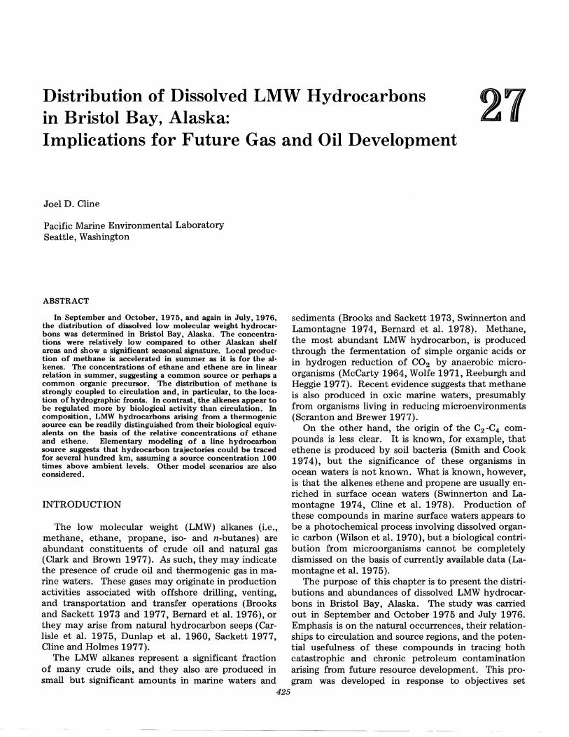
Figure 27-1. Location of stations occupied in Bristol Bay in Sept.-Oct. 1975 and July 1976. The solid lines show the ver­tical sections along which the distribution of properties is discussed. Depth contours are in fathoms.

,measurements (24 hours and 36 hours) were made atStations Ebb 37 and 46 in September and October,1975. In addition to the sampling for dissolved hy­drocarbons, measurements of salinity, temperature,and concentrations of suspended matter were alsomade at each of the stations shown (Feely and Cline1977).

Methane

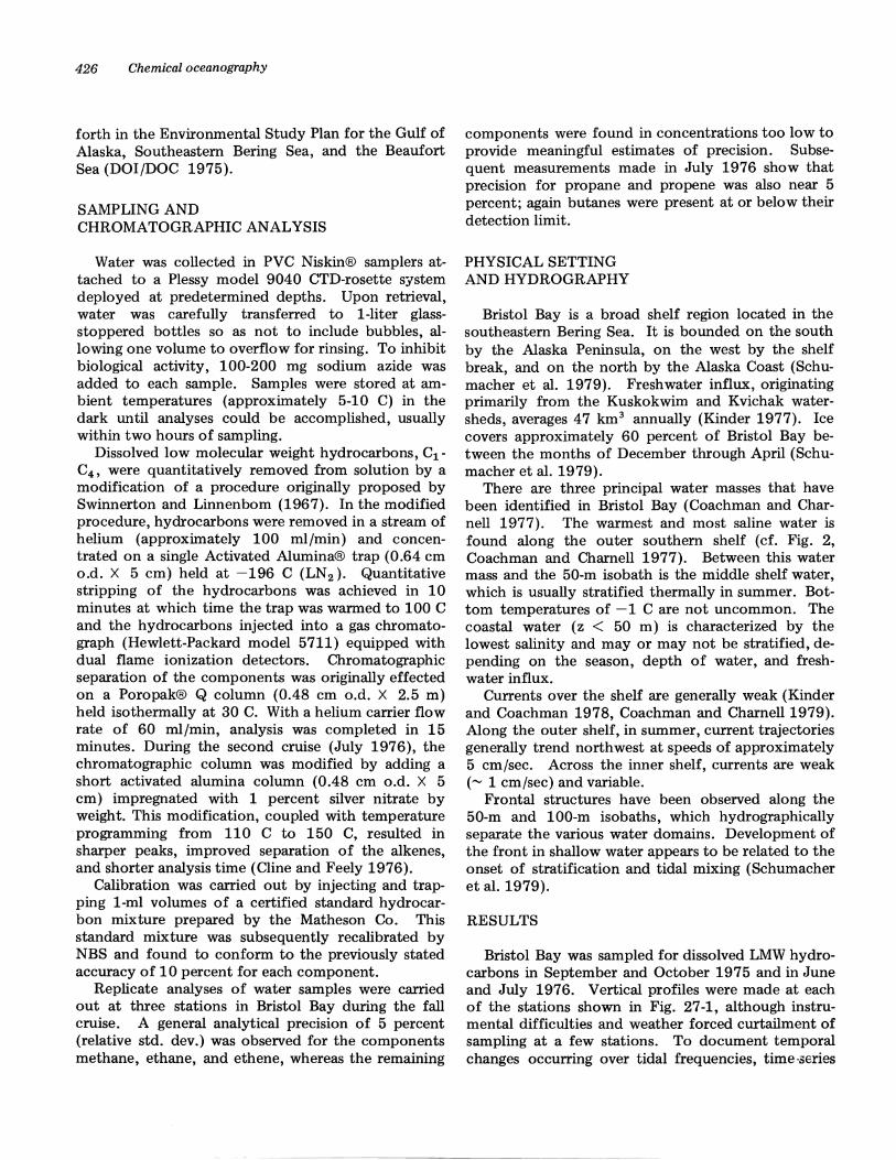
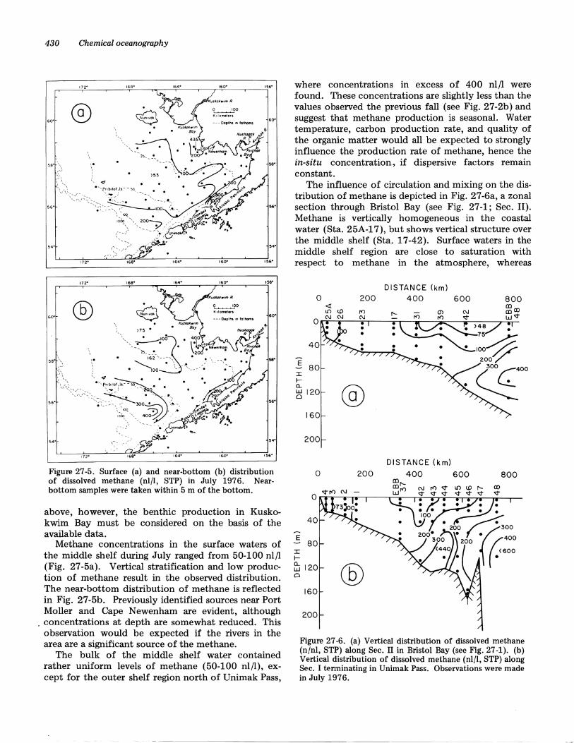
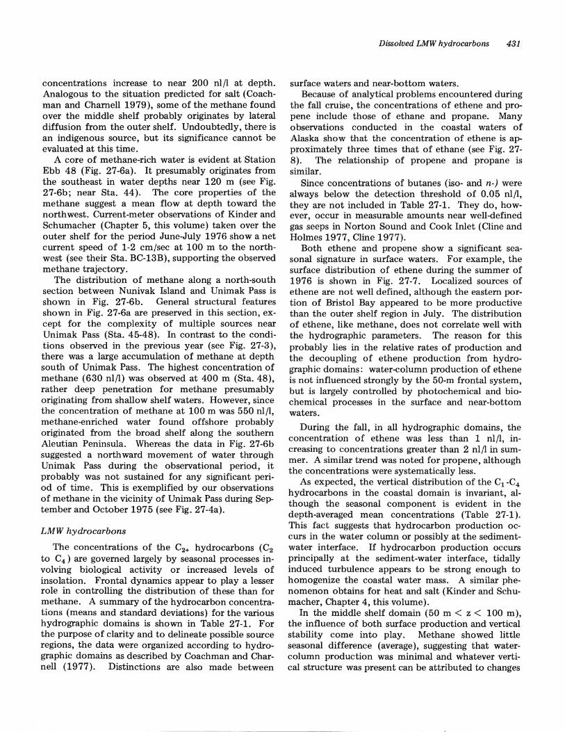
Methane is the dominant dissolved LMW hydrocar­bon and its distribution reflects both seasonal andspatial source patterns. The distributions of dissolvedmethane in surface and near-bottom waters are shownin Figs. 27-2a and b for September and October1975. Except for a localized source near Port Moller,

surface c.oncentrations of methane were near valuesexpected from the saturation of air. Assuming amethane partial pressure of 1.4 ppm(v) (Ehhalt 1974)and a mean surface temperature and salinity of 7 Cand 310 100 (Kinder and Schumacher, Chapter 4, thisvolume), the equilibrium solubility concentration ofCH4 is 53 ± 3 nlfl (STP) (Yamamoto et ale 1976).The plume of methane observed south of Cape New­enham may have arisen from the Nushagak and Kvi­chak Rivers, although the small enrichment noted (75nlll < CH4 < 94 nl/l) is near the ambient noise levelwhen variability in time and space is taken into ac­count. These data, however, do not rule out a con­tribution from bottom sediments in the KuskokwimDelta.

428 Chemical oceanography

Figure 27-2. Surface (a) and near-bottom (b) distributionsof dissolved methane (nl/l, STP) in Sept.-Oct. 1975. Near­bottom samples were taken within 5 m of the bottom.

The elevated concentrations near Port Moller pre­sumably arise from the tidal discharge of methane­rich waters from the lagoon. It is interesting,however, that methane is contained inside the 50-misobath. The lack of a definite plume trajectoryeither east or west also suggests that there was littleor no persistent coastal current at the time of thesemeasurements. This is in general agreement with cir­culation studies carried out in Bristol Bay over thepast several years (Kinder and Schumacher, Chapter5, this volume), in which wind forcing or other mete­orological events may give rise to a coastal current.The strong lateral methane gradient in the absence ofany significant mean flow also suggests that the pre­viously described frontal system along the 50-m iso-

bath (Schumacher et al. 1979) inhibits a horizontalflux of methane to the north.

The concentration of methane within 5 m of thebottom is shown in Fig. 27-2b. The most strikingfeature is the concentrated source over the outershelf, referred to here as St. George Basin. Concen­trations of methane near the bottom were in excessof 600 nl/l (STP) and represent approximately 12­fold supersaturation with respect to the atmosphere.The source of the methane is undoubtedly microbial,presumably arising from the activities of micro­organisms at the sediment-water interface. Accordingto Sharma (1979), bottom sediments along the outershelf are fine grained, containing more than 0.5 per­cent organic carbon by weight. While these concen­trations of carbon are not inordinately high, they areenriched compared to the inner shelf region, whereconcentrations range from 0.05 percent to 0.2 per­cent (Sharma 1979). The exception to this generali­zation is Kuskokwim Bay, where organic carbonconcentrations range from 0.1 percent to 0.5 percent.These fine-grained sediments also are a likely sour,ceof methane, as mentioned earlier.

The methane distribution inside the 50-m isobathwas vertically homogeneous. This distribution is ex­pected if the bottom production rates are small com­pared to the rate of vertical mixing. Salt and heatwere also vertically homogeneous in the coastalwater, suggesting strong vertical mixing at the time ofthe measurements (Kinder and Schumacher, Chapter4, this volume). For the sake of brevity, the distribu­tions of salinity and temperature for that period willnot be shown as they were similar to those observedby Schumacher et al. (1979) for the following year.

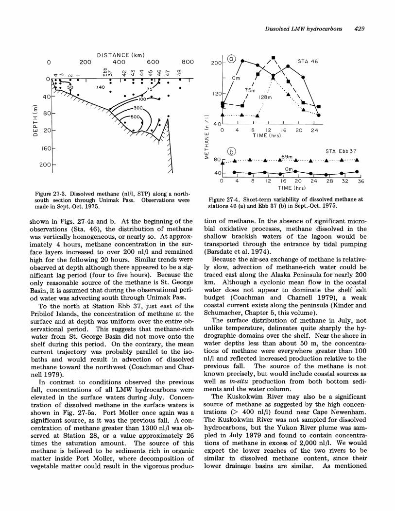
In Bristol Bay, the distribution of methane is con­trolled by several point sources and circulation. Thisis apparent in Fig. 27-3, where the vertical distribu­tion of methane is shown along a north-south sectionbetween Nunivak Island and Unimak Pass (see Fig.27-1; Sec. I). Methane in St. George Basin clearlyoriginates from the bottom. While a weak meancurrent over the outer shelf (Kinder and Schumacher,Chapter 5, this volume) may transport methane tothe northwest, this figure clearly shows the influenceof vertical mixing on the distribution of methane.Because of increased vertical turbulence, methane­rich water was observed at the surface near UnimakPass (Sta. 46). In contrast, the inner shelf region wasnearly homogeneous with respect to dissolved meth­ane, with concentrations near the equilibrium values.

In order to evaluate the short-term variability ofmethane, Stations 46 and Ebb 37 were sampled every4 hours for 24 hours and 36 hours respectively.The results of the time-series measurements are

60·

1600

.~~>45

• Kuskokwim

~ • / Boy

• ""-50.

>48

®

600

Dissolved LMW hydrocarbons 429

Figure 27-3. Dissolved methane (nl/l, STP) along a north­south section through Unimak Pass. Observations weremade in Sept.-Oct. 1975.

2420

•/ \ STA 46\

\

.~". \

128m A. \

". --8 12 16TIM E (hrs)

4

Om

®

·······6· ..

200

wZ<tI

~ (5) STA Ebb 37~ 69m

80f....• ·· ··· ·· ..A···· ···· · .. ·· ·· ...

40t ~ -, "I ~, -, -I ,o 4 8 12 16 20 24 28 32 36

TIME (hrs)

::::: 40~-.l....--_...L...-_...L...-_..1..-_.....L.--_....L.......-

.5 0

Figure 27-4. Short-term variability of dissolved methane atstations 46 (a) and Ebb 37 (b) in Sept.-Oct. 1975.

800DISTANCE (km)

400 600200

80

40

o

160

200

E

::r:r­a..w 120o

shown in Figs. 27-4a and b. At the beginning of theobservations (Sta. 46), the distribution of methanewas vertically homogeneous, or nearly so. At approx­imately 4 hours, methane concentration in the sur­face layers increased to over 200 nl/l and remainedhigh for the following 20 hours. Similar trends wereobserved at depth although there appeared to be a sig­nificant lag period (four to five hours). Because theonly reasonable source of the methane is St. GeorgeBasin, it is assumed that during the observational peri­od water was advecting south through Unimak Pass.

To the north at Station Ebb 37, just east of thePribilof Islands, the concentration of methane at thesurface and at depth was uniform over the entire ob­servational period. This suggests that methane-richwater from St. George Basin did not move onto theshelf during this period. On the contrary, the meancurrent trajectory was probably parallel to the iso­baths and would result in advection of dissolvedmethane toward the northwest (Coachman and Char­nell 1979).

In contrast to conditions observed the previousfall, concentrations of all LMW hydrocarbons wereelevated in the surface waters during July. Concen­tration of dissolved methane in the surface waters isshown in Fig. 27-5a. Port Moller once again was asignificant source, as it was the previous fall. A con­centration of methane greater than 1300 nl/l was ob­served at Station 28, or a value approximately 26times the saturation amount. The source of thismethane is believed to be sediments rich in organicmatter inside Port Moller, where decomposition ofvegetable matter could result in the vigorous produc-

tion of methane. In the absence of significant micro­bial oxidative processes, methane dissolved in theshallow brackish waters of the lagoon would betransported through the entrance by tidal pumping(Barsdate et al. 1974).

Because the air-sea exchange of methane is relative­ly slow, advection of methane-rich water could betraced east along the Alaska Peninsula for nearly 200km. Although a cyclonic mean flow in the coastalwater does not appear to dominate the shelf 'saltbudget (Coachman and Charnell 1979), a weakcoastal current exists along the peninsula (Kinder andSchumacher, Chapter 5, this volume).

The surface distribution of methane in July, notunlike temperature, delineates quite sharply the hy­drographic domains over the shelf. Near the shore inwater depths less than about 50 m, the concentra­tions of methane were everywhere greater than 100nlll and reflected increased production relative to theprevious fall. The source of the methane is notknown precisely, but would include coastal sources aswell as in-situ production from both bottom sedi­ments and the water column.

The Kuskokwim River may also be a significantsource of methane as suggested by the high concen­trations (> 400 nl/l) found near Cape Newenham.The Kuskokwim River was not sampled for dissolvedhydrocarbons, but the Yukon River plume was sam­pled in July 1979 and found to contain concentra­tions of methane in excess of 2,000 nl/l. We wouldexpect the lower reaches of the two rivers to besimilar in dissolved methane content, since theirlower drainage basins are similar. As mentioned

430 Chemical oceanography

DISTANCE (km)

0 200 400 600 800<{ CD 00L{) <.D r-- (j) C\J

~q0

C\J C\J r<> r0 q

~487:1• 75~

40 •• • • 100~•

E • 20080

• • ~oo:r:r-a..

@~ 120

160

200

where concentrations in excess of 400 nl/l werefound. These concentrations are slightly less than thevalues observed the previous fall (see Fig. 27-2b) andsuggest that methane production is seasonal. Watertemperature, carbon production rate, and quality ofthe organic matter would all be expected to stronglyinfluence the production rate of methane, hence thein-situ concentration., if dispersive factors remainconstant.

The influence of circulation and mixing on the dis­tribution of methane is depicted in Fig. 27-6a, a zonalsection through Bristol Bay (see Fig. 27-1; Sec. II).Methane is vertically homogeneous in the coastalwater (Sta. 25A-17), but shows vertical structure overthe middle shelf (Sta. 17-42). Surface waters in themiddle shelf region are close to saturation withrespect to methane in the atmosphere, whereas172 0 168· 164·

1720 168· 164·

600 (§)

1720 1680 160· 156·

@) O'--J.-L--'---J........IOOK,lometers

600

--- Depths In fathoms60·

Figure 27-6. (a) Vertical distribution of dissolved methane(n/nl, STP) along Sec. II in Bristol Bay (see Fig. 27-1). (b)Vertical distribution of dissolved methane (nl/l, STP) alongSec. I terminating in Unimak Pass. Observations were madein July 1976.

800

DISTANCE (km)

400 600CDr--

~r0

200o

40

E80

:r:r-~ 120 @0

160

200

Figure 27-5. Surface (a) and near-bottom (b) distributionof dissolved methane (nl/l, STP) in July 1976. Near­bottom samples were taken within 5 m of the bottom.

172·

above, however, the benthic production in Kusko­kwim Bay must be considered on the basis of theavailable data.

Methane concentrations in the surface waters ofthe middle shelf during July ranged from 50-100 nl/l(Fig. 27-5a). Vertical stratification and low produc­tion of methane result in the observed distribution.The near-bottom distribution of methane is reflectedin Fig. 27-5b. Previously identified sources near PortMoller and Cape Newenham are evident, although

. concentrations at depth are somewhat reduced. Thisobservation would be expected if the rivers in thearea are a significant source of the methane.

The bulk of the middle shelf water containedrather uniform levels of methane (50-100 nl/l), ex­cept for the outer shelf region north of Unimak Pass,

concentrations increase to near 200 nlll at depth.Analogous to the situation predicted for salt (Coach­man and Charnell 1979), some of the methane foundover the middle shelf probably originates by lateraldiffusion from the outer shelf. Undoubtedly, there isan indigenous source, but its significance cannot beevaluated at this time.

A core of methane-rich water is evident at"StationEbb 48 (Fig. 27-6a). It presumably originates fromthe southeast in water depths near 120 m (see Fig.27-6b; near Sta. 44). The core properties of themethane suggest a mean flow at depth toward thenorthwest. Current-meter observations of Kinder andSchumacher (Chapter 5, this volume) taken over theouter shelf for the period June-July 1976 show a netcurrent speed of 1-2 cmlsec at 100 m to the north­west (see their Sta. BC-13B), supporting the observedmethane trajectory.

The distribution of methane along a north-southsection between Nunivak Island and Unimak Pass isshown in Fig. 27-6b. General structural featuresshown in Fig. 27-6a are preserved in this section, ex­cept for the complexity of multiple sources nearUnimak Pass (Sta. 45-48). In contrast to the condi­tions observed in the previous year (see Fig. 27-3),there was a large accumulation of methane at depthsouth of Unimak Pass. The highest concentration ofmethane (630 nl/l) was observed at 400 m (Sta. 48),rather deep penetration for methane presumablyoriginating from shallow shelf waters. However, sincethe concentration of methane at 100 m was 550 nlll,methane-enriched water found offshore probablyoriginated from the broad shelf along the southernAleutian Peninsula. Whereas the data in Fig. 27-6bsuggested a northward movement of water throughUnimak Pass during the observational period, itprobably was not sustained for any significant peri­od of time. This is exemplified by our observationsof methane in the vicinity of Unimak Pass during Sep­tember and October 1975 (see Fig. 27-4a).

LMW hydrocarbons

The concentrations of the C2+ hydrocarbons (C2

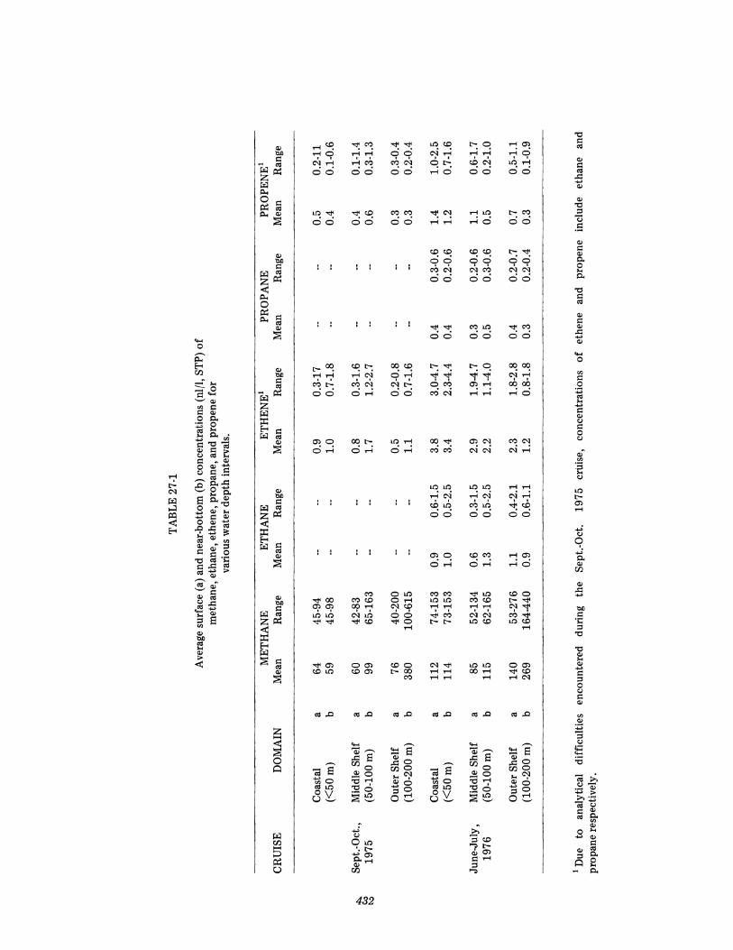
to C4 ) are governed largely by seasonal processes in­volving biological activity or increased levels ofinsolation. Frontal dynamics appear to play a lesserrole in controlling the distribution of these than formethane. A summary of the hydrocarbon concentra­tions (means and standard deviations) for the varioushydrographic domains is shown in Table 27-1. Forthe purpose of clarity and to delineate possible sourceregions, the data were organized according to hydro­graphic domains as described by Coachman and Char­nell (1977). Distinctions are also made between

Dissolved LMW hydrocarbons 431

surface waters and near-bottom waters.Because of analytical problems encountered during

the fall cruise, the concentrations of ethene and pro­pene include those of ethane and propane. Manyobservations conducted in the coastal waters ofAlaska show that the concentration of ethene is ap­proximately three times that of ethane (see Fig. 27­8). The relationship of propene and propane issimilar.

Since concentrations of butanes (iso- and n-) werealways below the detection threshold of 0.05 nlll,they are not included in Table 27-1. They do, how­ever, occur in measurable amounts near well-definedgas seeps in Norton Sound and Cook Inlet (Cline andHolmes 1977, Cline 1977).

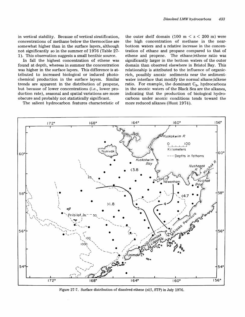
Both ethene and propene show a significant sea­sonal signature in surface waters. For example, thesurface distribution of ethene during the summer of1976 is shown in Fig. 27-7. Localized sources ofethene are not well defined, although the eastern por­tion of Bristol Bay appeared to be more productivethan the outer shelf region in July. The distributionof ethene, like methane, does not correlate well withthe hydrographic parameters. The reason for thisprobably lies in the relative rates of production andthe decoupling of ethene production from hydro­graphic domains: water-column production of etheneis not influenced strongly by the 50-m frontal system,but is largely controlled by photochemical and bio­chemical processes in the surface and near-bottomwaters.

During the fall, in all hydrographic domains, theconcentration of ethene was less than 1 nlll, in­creasing to concentrations greater than 2 nlll in sum­mer. A similar trend was noted for propene, althoughthe concentrations were systematically less.

As expected, the vertical distribution of the C1 -C4

hydrocarbons in the coastal domain is invariant, al­though the seasonal component is evident in thedepth-averaged mean concentrations (Table 27-1).This fact suggests that hydrocarbon production oc­curs in the water column or possibly at the sediment­water interface. If hydrocarbon production occursprincipally at the sediment-water interface, tidallyinduced turbulence appears to be strong enough tohomogenize the coastal water mass. A similar phe­nomenon obtains for heat and salt (Kinder and Schu­macher, Chapter 4, this volume).

In the middle shelf domain (50 m < z < 100 m),the influence of both surface production and verticalstability come into play. Methane showed littleseasonal difference (average), suggesting that water­column production was minimal and whatever verti­cal structure was present can be attributed to changes

TA

BL

E27

-1

Ave

rage

surf

ace

(a)

and

near

-bot

tom

(b)

conc

entr

atio

ns(n

l/l,

STP)

of

met

hane

,et

hane

,eth

ene,

prop

ane,

and

prop

ene

for

vari

ous

wat

erde

pth

inte

rval

s.

ME

TH

AN

EE

TH

AN

EE

TH

EN

El

PRO

PAN

EPR

OPE

NE

l

CR

UIS

ED

OM

AIN

Mea

nR

ange

Mea

nR

ange

Mea

nR

ange

Mea

nR

ange

Mea

nR

ange

Coa

stal

a64

45-9

4--

--0.

90.

3-17

----

0.5

0.2-

11«

50

m)

b59

45-9

8--

--1.

00.

7-1.

8--

--0.

40.

1-0.

6

~S

ept.-

Oct

.,M

iddl

eS

helf

a60

42-8

3--

--0.

80.

3-1.

6--

--0.

40.

1-1.

4~

1975

(50-

100

m)

b99

65-1

63--

--1.

71.

2-2.

7--

--0.

60.

3-1.

3

Out

erS

helf

a76

40-2

00--

--0.

50.

2-0.

8--

--0.

30.

3-0.

4(1

00-2

00m

)b

380

100-

615

----

1.1

0.7-

1.6

----

0.3

0.2-

0.4

Coa

stal

a11

274

-153

0.9

0.6-

1.5

3.8

3.0-

4.7

0.4

0.3-

0.6

1.4

1.0-

2.5

«5

0m

)b

114

73-1

531.

00.

5-2.

53.

42.

3-4.

40.

40.

2-0.

61.

20.

7-1.

6

June

-Jul

y,M

iddl

eS

helf

a85

52-1

340.

60.

3-1.

52.

91.

9-4.

70.

30.

2-0.

61.

10.

6-1.

719

76(5

0-10

0m

)b

115

62-1

651.

30.

5-2.

52.

21.

1-4.

00.

50.

3-0.

60.

50.

2-1.

0

Out

erS

helf

a14

053

-276

1.1

0.4-

2.1

2.3

1.8-

2.8

0.4

0.2-

0.7

0.7

0.5-

1.1

(100

-200

m)

b26

916

4-44

00.

90.

6-1.

11.

20.

8-1.

80.

30.

2-0.

40.

30.

1-0.

9

1D

ueto

anal

ytic

aldi

ffic

ulti

esen

coun

tere

ddu

ring

the

Sep

t.-O

ct.

1975

crui

se,

conc

entr

atio

nso

fet

hene

and

prop

ene

incl

ude

etha

nean

dpr

opan

ere

spec

tive

ly.

Dissolved LMW hydrocarbons 433

in vertical stability. Because of vertical stratification,concentrations of methane below the thermocline aresomewhat higher than in the surface layers, althoughnot significantly so in the summer of 1976 (Table 27­1). This observation suggests a small benthic source.

In fall the highest concentration of ethene wasfound at depth, whereas in summer the concentrationwas higher in the surface layers. This difference is at­tributed to increased biological or induced photo­chemical production in the surface layers. Similartrends are apparent in the distribution of propene,but because of lower concentrations (i.e., lower pro­duction rate), seasonal and spatial variations are moreobscure and probably not statistically significant.

The salient hydrocarbon features characteristic of

the outer shelf domain (100 m < z < 200 m) werethe high concentration of methane in the near­bottom waters and a relative increase in the concen­tration of ethane and propane compared to that ofethene and propene. The ethane/ethene ratio wassignificantly larger in the bottom waters of the outerdomain than observed elsewhere in Bristol Bay. Thisrelationship is attributed to the influence of organic­rich, possibly anoxic sediments near the sediment­water interface that modify the normal alkane /alkeneratio. For example, the dominant C2+ hydrocarbonsin the anoxic waters of the Black Sea are the alkanes,indicating that the production of biological hydro­carbons under anoxic conditions tends toward themore reduced alkanes (Hunt 1974).

K i lometers

a 100I I I I I ,

--- Depths in fathoms

• ,¢ap~4 '.' .~. Newenha~

••

<3.8

••

•

•

•

•

•

••

>I. 8

•

•

•

•

•

••

\\\

•

~•

Figure 27 -7. Surface distribution of dissolved ethene (nI/I, STP) in July 1976.

434 Chemical oceanography

5

(0)

4

2

3

2 3Ethene (nl/l)

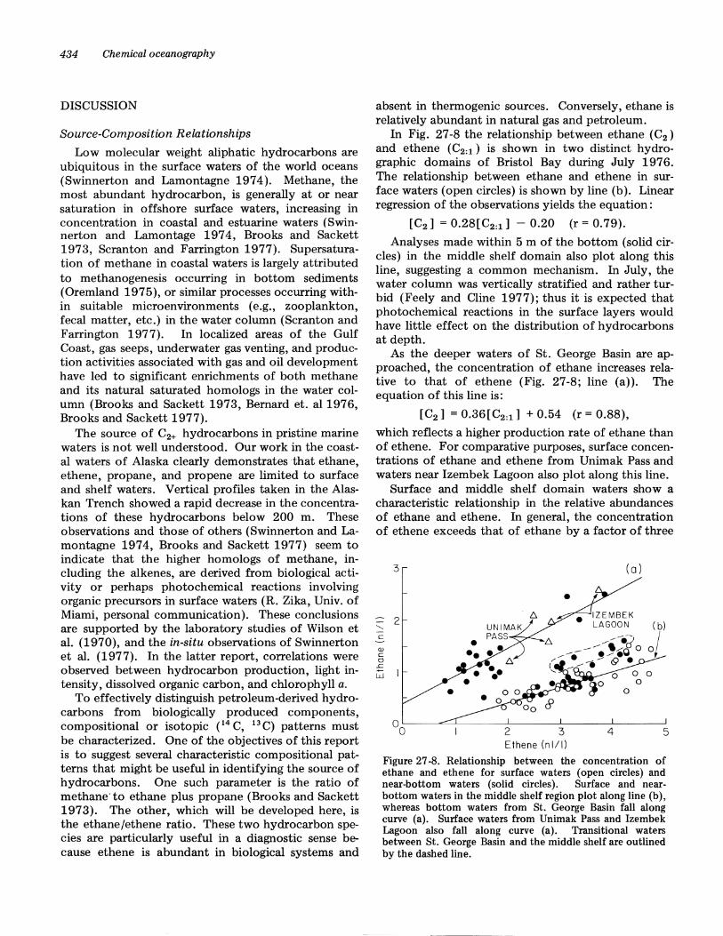
Figure 27 -8. Relationship between the concentration ofethane and ethene for surface waters (open. circles) andnear-bottom waters (solid circles). Surface and near­bottom waters in the middle shelf region plot along line (b),whereas bottom waters from St. George Basin fall alongcurve (a). Surface waters from Unimak Pass and IzembekLagoon also fall along curve (a). Transitional watersbetween St. George Basin and the middle shelf are outlinedby the dashed line.

absent in thermogenic sources. Conversely, ethane isrelatively abundant in natural gas and petroleum.

In Fig. 27-8 the relationship between ethane (C2 )

and ethene (C2 :1 ) is shown in two distinct hydro­graphic domains of Bristol Bay during July 1976.The relationship between ethane and ethene in sur­face waters (open circles) is shown by line (b). Linearregression of the observations yields the equation:

[C2 ] = 0.28[C2 :1 ] - 0.20 (r = 0.79).

Analyses made within 5 m of the bottom (solid cir­cles) in the middle shelf domain also plot along thisline, suggesting a common mechanism. In July, thewater column was vertically stratified and rather tur­bid (Feely and Cline 1977); thus it is expected thatphotochemical reactions in the surface layers wouldhave little effect on the distribution of hydrocarbonsat depth.

As the deeper waters of St. George Basin are ap­proached, the concentration of ethane increases rela­tive to that of ethene (Fig. 27-8; line (a)). Theequation of this line is:

[C2 ] = 0.36[C2 :1 ] + 0.54 (r = 0.88),

which reflects a higher production rate of ethane thanof ethene. For comparative purposes, surface concen­trations of ethane and ethene from Unimak Pass andwaters near Izembek Lagoon also plot along this line.

Surface and middle shelf domain waters show acharacteristic relationship in the relative abundancesof ethane and ethene. In general, the concentrationof ethene exceeds that of ethane by a factor of three

"-..

-5())

co

..c

W

DISCUSSION

Source-Composition Relationships

Low molecular weight aliphatic hydrocarbons areubiquitous in the surface waters of the world oceans(Swinnerton and Lamontagne 1974). Methane, themost abundant hydrocarbon, is generally at or nearsaturation in offshore surface waters, increasing inconcentration in coastal and estuarine waters (Swin­nerton and Lamontage 1974, Brooks and Sackett1973, Scranton and Farrington 1977). Supersatura­tion of methane in coastal waters is largely attributedto methanogenesis occurring in bottom sediments(Oremland 1975), or similar processes occurring with­in suitable microenvironments (e.g., zooplankton,fecal matter, etc.) in the water column (Scranton andFarrington 1977). In localized areas of the GulfCoast, gas seeps, underwater gas venting, and produc­tion activities associated with gas and oil developmenthave led to significant enrichments of both methaneand its natural saturated homologs in the water col­umn (Brooks and Sackett 1973, Bernard et. a11976,Brooks and Sackett 1977).

The source of C2+ hydrocarbons in pristine marinewaters is not well understood. Our work in the coast­al waters of Alaska clearly demo'nstrates -that ethane,ethene, propane, and propene are limited to surfaceand shelf waters. Vertical profiles taken in the Alas­kan Trench showed a rapid decrease in the concentra­tions of these hydrocarbons below 200 m. Theseobservations and those of others (Swinnerton and La­montagne 1974, Brooks and Sackett 1977) seem toindicate that the higher homologs of methane, in­cluding the alkenes, are derived from biological acti­vity or perhaps photochemical reactions involvingorganic precursors in surface waters (R. Zika, Univ. ofMiami, personal communication). These conclusionsare supported by the laboratory studies of Wilson etal. (1970), and the in-situ observations of Swinnertonet ale (1977). In the latter report, correlations wereobserved between hydrocarbon production, light in­tensity, dissolved organic carbon, and chlorophyll a.

To effectively distinguish petroleum-derived hydro­carbons from biologically produced components,compositional or isotopic (14 C, 13 C) patterns mustbe characterized. One of the objectives of this reportis to· suggest several characteristic compositional pat­terns that might be useful in identifying the source ofhydrocarbons. One such parameter is the ratio ofmethane· to ethane plus propane (Brooks and Sackett1973). The other, which will be developed here, isthe ethane/ethene ratio. These two hydrocarbon spe­cies are particularly useful in a diagnostic sense be­cause ethene is abundant in biological systems and

Dissolved LMW hydrocarbons 435

[4] [4]A + «1-X)/X)[4 ]T[~ ] +[Ca ] = [~] A + [Ca ] A + « 1 - x) /x)[~ ] T +[ Ca ] T

(1)[~] [~]A [~]T

[~:l] = [C2:1 ]A + «l-x)/x) [~:l]A (2)

The fraction of ambient water is x, whereas con­centrations of the individual hydrocarbons are shownin brackets. The two sources, between which mixing

SA~k~~~~~I~ / !FLUID :

10° I

10-1 101 102 103 104

[C2]/[C 2:1]

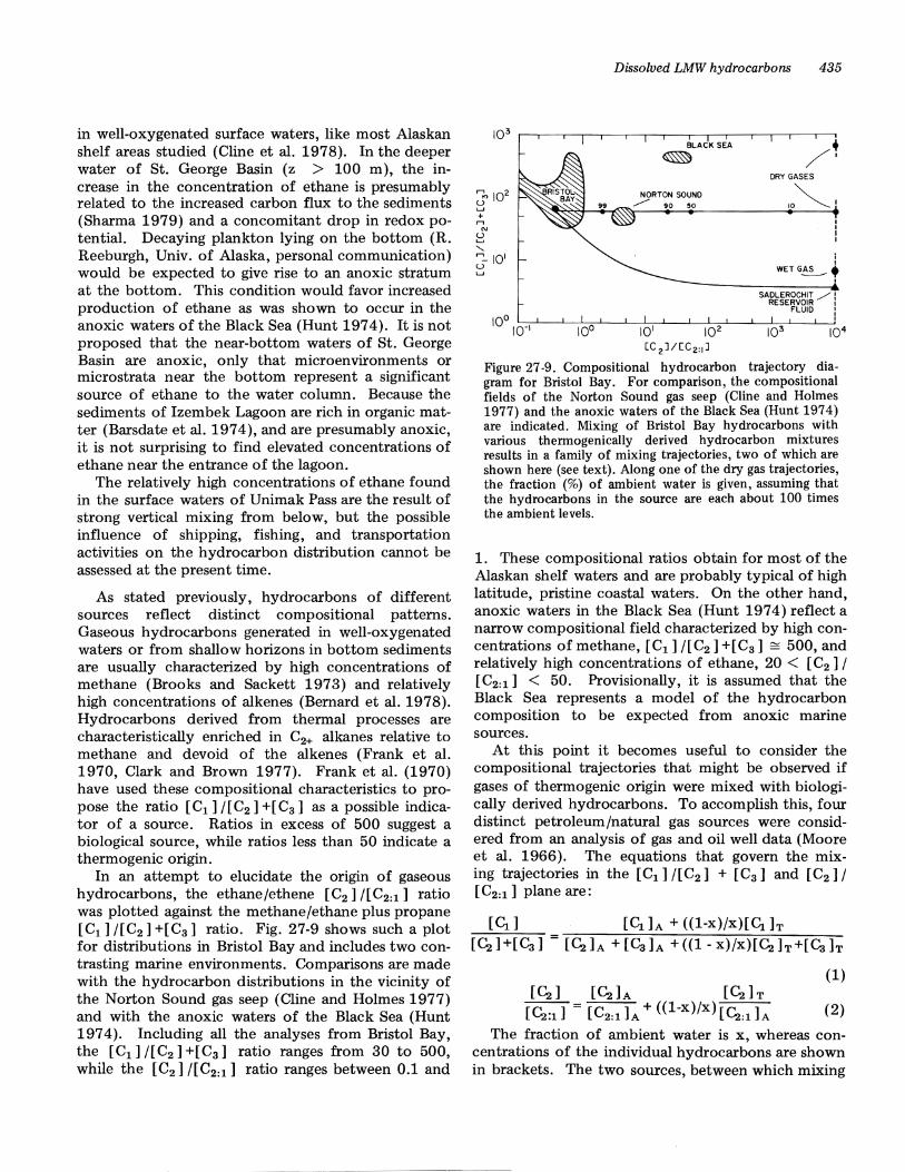
Figure 27-9. Compositional hydrocarbon trajectory dia­gram for Bristol Bay. For comparison, the compositionalfields of the Norton Sound gas seep (Cline and Holmes1977) and the anoxic waters of the Black Sea (Hunt 1974)are indicated. Mixing of Bristol Bay hydrocarbons withvarious thermogenically derived hydrocarbon mixturesresults in a family of mixing trajectories, two of which areshown here (see text). Along one of the dry gas trajectories,the fraction (%) of ambient water is given, assuming thatthe hydrocarbons in the source are each about 100 timesthe ambient levels.

I,WETG~'

DRY GASES

IO~'NORTON SOUND~ 90 50

S 102

L.J

+.,C\I

8"~-IOIL.J

1. These compositional ratios obtain for most of theAlaskan shelf waters and are probably typical of highlatitude, pristine coastal waters. On the other hand,anoxic waters in the Black Sea (Hunt 1974) reflect anarrow compositional field characterized by high con­centrations of methane, [C1 ] /[C2 ] +[Ca ] 3:: 500, andrelatively high concentrations of ethane, 20 < [C2 ] /

[C2 :1 ] < 50. Provisionally, it is assumed that theBlack Sea represents a model of the hydrocarboncomposition to be expected from anoxic marinesources.

At this point it becomes useful to consider thecompositional trajectories that might be observed ifgases of thermogenic origin were mixed with biologi­cally derived hydrocarbons. To accomplish this, fourdistinct petroleum/natural gas sources were consid­ered from an analysis of gas and oil well data (Mooreet ale 1966). The equations that govern the mix­ing trajectories in the [C1 ] /[C2 ] + [Ca ] and [C2 ] /

[C2 :1 ] plane are:

in well-oxygenated surface waters, like most Alaskanshelf areas studied (Cline et ale 1978). In the deeperwater of St. George Basin (z > 100 m), the in­crease in the concentration of ethane is presumablyrelated to the increased carbon flux to the sediments(Sharma 1979) and a concomitant drop in redox po­tential. Decaying plankton lying on the bottom (R.Reeburgh, Univ. of Alaska, personal communication)would be expected to give rise to an anoxic stratumat the bottom. This condition would favor increasedproduction of ethane as was shown to occur in theanoxic waters of the Black Sea (Hunt 1974). It is notproposed that the near-bottom waters of St. GeorgeBasin are anoxic, only that microenvironments ormicrostrata near the bottom represent a significantsource of ethane to the water column. Because thesediments of Izembek Lagoon are rich in organic mat­ter (Barsdate et ale 1974), and are presumably anoxic,it is not surprising to find elevated concentrations ofethane near the entrance of the lagoon.

The relatively high concentrations of ethane foundin the surface waters of Unimak Pass are the result ofstrong vertical mixing from below, but the possibleinfluence of shipping, fishing, and transportationactivities on the hydrocarbon distribution cannot beassessed at the present time.

As stated previously, hydrocarbons of differentsources reflect distinct compositional patterns.Gaseous hydrocarbons generated in well-oxygenatedwaters or from shallow horizons in bottom sedimentsare usually characterized by high concentrations ofmethane (Brooks and Sackett 1973) and relativelyhigh concentrations of alkenes (Bernard et ale 1978).Hydrocarbons derived from thermal processes arecharacteristically enriched in C2+ alkanes relative tomethane and devoid of the alkenes (Frank et al.1970, Clark and Brown 1977). Frank et ale (1970)have used these compositional characteristics to pro­pose the ratio [C1 ] /[C2 ] +[Ca ] as a possible indica­tor of a source. Ratios in excess of 500 suggest abiological source, while ratios less than 50 indicate athermogenic origin.

In an attempt to elucidate the origin of gaseoushydrocarbons, the ethane/ethene [C2 ] /[C2:1 ] ratiowas plotted against the methane/ethane plus propane[C1 ]/[C2 ]+[Ca ] ratio. Fig. 27-9 shows such a plotfor distributions in Bristol Bay and includes two con­trasting marine environments. Comparisons are madewith the hydrocarbon distributions in the vicinity ofthe Norton Sound gas seep (Cline and Holmes 1977)and with the anoxic waters of the Black Sea (Hunt1974). Including all the analyses from Bristol Bay,the [C1 ]/[C2 ]+[Ca ] ratio ranges from 30 to 500,while the [C2 ] /[C2:1 ] ratio ranges between 0.1 and

436 Chemical oceanography

TABLE 27-2.

3.7

{31 = 0.04 ml CH4 (STP}jml H2 0{32 = 0.06 ml C2 H6 (STP}jml H2 0{33 = 0.06 ml C3 Hs (STP}jml H2 0

0.0300.051

Mole FractionC1 C2 Ca

0.44

D 1 = 0.85 X lOS cm2 jsecD2 = 0.69 X 105 cm2 jsecD 3 = 0.55 X lOS cm2 jsec

TABLE 27-3.

where JJi' Di, and Pi represent the Bunsen coefficient,diffusion coefficient, and mole fraction of (1) meth­ane, (2) ethane, and (3) propane. Assuming a meantemperature and salinity of 5 C and 300 100,

Mole fractions of methane, ethane, and propane fromthe reservoir fluid of the Sadlerochit formation,

Prudhoe Bay (Anon. 1971), and the resultingequilibrium solubility ratio. Gas phase was assumed to

contain only C1 -C4 hydrocarbons, nitrogen,carbon dioxide, and helium.

Bunsen coefficients ({3i), corrected for the "saltingout effect" and the molecular diffusion coefficients(Di ), not corrected for the ionic strength of seawater,were estimated from the data of Bonoli and Wither­spoon (1968). The solubility ratio, [C1 ]' I[C2 ]'+[Ca ] " for gas well data calculated from equation 3,is shown in Table 27-2 and is also shown as mixingend members in Fig. 27-9. Because it has been as­sumed that the concentration of ethene is zero (Le.,[C2 ]'/[C2 :1 ]' + 00), the mixing end members are lo­cated at the extreme right margin.

The remaining end member we wish to consider isa wet gas associated with petroleum. For this pur­pose, the volatile fraction from the reservoir fluid ofthe Sadlerochit formation, Prudhoe Bay, was selected(Anon. 1971). The so-called volatile fraction, C1 toC4 hydrocarbons plus air gases, was normalized to100 percent and the partial pressures of methane,ethane, and propane were calculated. As in the ex­ample given earlier, a gas of this composition is equil­ibrated with a parcel of Bristol Bay water. Table 27­3 gives the mole fraction composition of the gasphase and the resulting equilibrium solubility ratio.Bunsen coefficients and diffusion coefficients werethe same as before.

As expected, the gas is relatively rich in C2+ hydro­carbons and its composition is similar to that calcula­ted earlier for a wet gas derived from gas wells. Ofthe gases present in the normalized mixture, methane,ethane, and propane constituted 81.6 percent by vol-

(3)

Wet GasDry Gas"Very"Dry Gas

Definition

[C; ] , JJI D1 PI

[~]' + [Ca ]' = JJ2 D2P2 + JJaDaPa

Mean mole fraction of methane, ethane, and propane,calculated for three arbitrarily defined natural gas fractions

(Moore et a1. 1966). Number of samples used in eachstatistic calculation is shown in column 5. Standard deviation

about the mean is shown in parentheses.

Mole Fraction [C1 ]

Ct ~ Ca [C2 ]+[Ca ]n

.79(.11) .075(.04) .033(.026) 7 313

.96(.02) .011(.005) .002(.002) 61 47

.98(.02) .001(.0006) Tr 672 6

The actual concentration ratio observed in thewater will depend on the component partial pressure(or mole fraction), the Bunsen coefficient, which de­pends upon salinity and temperature, and the depthof water at which gas injection occurs. Implicit in theprevious statement is that equilibrium is achieved be­tween the gaseous and aqueous phases and that therate of solution of the gases is a function of thethickness of the stagnant film boundary layer(Broecker and Peng 1974). Actually, equilibrium isprobably not achieved. However, because the Bunsencoefficients and diffusion coefficients are similar formethane, ethane, and propane, the solubility ratiowill not be significantly different from the equilib­rium ratio. If these minimum conditions hold, thefollowing expression relates the component partialpressure in the gas phase to the equilibrium solubilityratio:

is assumed to occur, are indicated by the subscripts A(ambient) and T (thermogenic source). The implicitassumptions are that the source ratios are constantand that the concentration of ethene in the naturalgas source is zero.

To develop possible mixing scenarios, it was neces­sary to evaluate the possible ra.nge of LMW hydrocar­bon mixtures that might occur as the result ofoffshore production. The [C1 ] I [C2 ] +[Ca ] fre­quency diagram for 366 terrestrial gas wells (Moore etal. 1966) was plotted, and by this means three dis­crete compositions, identified on the basis of their[C1 ] I [C2 ] +[Ca ] ratio, were defined, ranging fromwhat is described as a ''very'' dry gas (methane rich)to a "typical" wet gas (methane poor). Some of thewet gases were associated with petroleum. A sum­mary of the calculations is shown in Table 27-2.

ume, C4 hydrocarbons amounted to 3.4 percent, CO2

was 14.2 percent, and the remaining 0.7 percent wasdivided between N2 and He. Having estimated somepossible petroleum and natural gas end members, tra­jectories that would result from mixing these endmembers with Bristol Bay water can be examined.The mixing trajectory resulting from the injection ofa typical dry gas will be considered first.

To simplify the calculation, it is assumed that am­bient Bering Sea water contains approximately thefollowing concentrations of LMW alkanes: [C1 ] =100 nl/l, [C2 ] = 1 nl/l, [C2 :1 ] = 3 nl/l, and [C3 ] =0.4 nl/l, giving a [C1 ] /[C2 ] +[C3 ] ratio of 71 and a[C2 ] /[C2 :1 ] ratio of approximately 0.33. It is appar­ent that this locus may be biased toward low valuesof the [C1 ]![C2 ]+[C3 ] ratio (Fig. 27-9). If weassume that the local source of hydrocarbons is100 times the ambient levels, the resulting mixingtrajectory, computed from equations 1 and 2, isshown in Fig. 27-9. The values above the solid circlesrepresent the percentage of ambient water at thosepoints. Mixing a gas of this composition with the am­bient water results in little change in the [C1 ] /

[C2 ] +[Cg ] ratio, but a large shift in the [C2 ] /

[C2 :1 ] ratio. This results directly from the assump­tion that the concentration of ethene was zero in thenatural gas source. It is interesting that the mixingline passes through the compositional field observedin the region of the Norton Sound gas seep (Cline andHolmes 1977). Conclusions as to the source of ther­mogenic hydrocarbon gases in Norton Sound on thebasis of this diagram would be misleading, however,since the ambient [C1 ] / [ C2 ] +[Cg] ratio in NortonSound is significantly higher (~500) than the averagevalue assigned for Bristol Bay (~71).

One additional feature of the compositional fielddiagram (Fig. 27-9) is that the mixing line betweentwo defined sources is invariant with respect to thesource concentrations of the hydrocarbons, as long asthe ratios are fixed. This means that regardless of thesource strength, compositional changes due to mixingwill occur along the mixing line between the twosources. With the relative concentrations (Le., 100:1)chosen in the above example, seepage or leakage of adry gas in Bristol Bay would be observable to approx­imately 99 percent dilution. If the relative concen­tration ratio is increased to 1000 :1, the effect is ob­servable to 99.9 percent dilution.

Finally, we calculate the hypothetical mixing line,assuming a wet gas composition similar to that foundin the Sadlerochit formation. This trajectory is alsoreflected in Fig. 27-9 and lies significantly below thepreviously calculated dry gas curve.

General conclusions drawn from Fig. 27-9 are that

Dissolved LMW hydrocarbons 437

typical wet and dry gases should be readily distin­guishable from biologically produced hydrocarbonsusing a combination of the [C1 ] /[C2 ] +[Cg ] and[C2 ] /[C2:1 ] ratios. The composition of LMW hy­drocarbon mixtures characterized by [C1 ] /[C2 ] +[C3 ] < 20 and [C2 ] /[C2 :1 ] > 100 strongly suggeststhat they are thermally derived. The exception is amethane-rich dry gas, such as that produced currentlyfrom several \-vells in upper Cook Inlet (Kelly 1968).These gas wells contain methane in excess of 98 molepercent, only traces of ethane, and no measurablepropane. An injected gas of this composition, in alllikelihood, will not be distinguishable from the suiteof hydrocarbons formed biologically under anoxicconditions (e.g., in sediments, lagoon environments,anoxic waters). Consequently, a dry gas of thiscomposition would be interpreted as biogenic on thebasis of its [C1 ] /[C2 ] +[Cg ] and [C2 ] /[C2 :1 ] ratios.

Additional useful tracers include the [C2 ] /[Cg ]

ratio (Nikonov 1972) and the 0 13 C composition ofthe seep methane (Brooks et al. 1974, Bernard et al.1976). In the latter study, Bernard and coworkershave plotted the [) 13 C of the dissolved methaneagainst the [C1 ] /[C2 ] +[C3 ] ratio for a number ofgas seeps investigated along the Texas shelf. Biogenicmethane was found to be isotopically light (-600 /00

to -700 /00 vs. PDB), whereas methane derived fromthermogenic sources was significantly heavier at-400 /00 to -500 /00. In a similar study, Kvenvoldenet al. (1979) found the pore fluid methane at thelocus of the seep in Norton Sound to be isotopicallyheavy at -360 /00, suggesting a thermal source.

There is no doubt that the isotopic composition ofdissolved methane is an excellent diagnostic param­eter in identifying the origin of natural gas. However,usually the concentration of methane is so low as topreclude the use of isotopic fingerprinting, exceptwhere gas venting is vigorous (e.g., Bernard et al.1976). At low concentrations, the compositionalratios should be useful in identifying sources of hy­drocarbons and their spatial trajectories. Becausethese hydrocarbons are dissolved, they readily iden­tify the trajectories of other dissolved components,which may possess greater toxicity (e.g., benzene).

In the following discussion, attention will be givento the dispersion field of LMW hydrocarbons origi­nating from a localized source and some estimates ofthe areal diffusion and advection scales applicable toBristol Bay.

Dispersion model

The major advantages of using LMW hydrocarbonsas in-situ tracers of petroleum are related to theirrelatively high abundance in crude oil and natural gas

438 Chemical oceanography

C(x,Y) = lhCo exp(-kx/U)[erf«L/2+y)/V2"Ci; )+erf«L/2~)/V2"Ci;)]

(5)

-where Co is the vertically integrated concentration atx = 0, L is the length of the line source, and a y is re­lated to Ky through the equation Ky = (U/2)(da y2 /

dx). Equation 5 is given in terms of the concentra­tion at x = 0 rather than the production rate. Thiswas done because the input rate for a seep would bedifficult to quantify. Moreover, to our knowledgethe production rate of known submarine gas seeps hasnever been documented. Thus, the model is ex­pressed in terms of the concentration field, whichshould be easily measured. To simplify the discussionin terms of maximum trajectory scales, only the cen-

(8)

(9)

(10)k = D /Llz· h.

after substitution.In Bristol Bay, as in any body of water, the source

of gas may be at the surface or at depth. To dis­cuss dispersion scales under both these conditions wewill assume that (1) the source is at the surface and isconsequently influenced by air-sea exchange and (2)the source is at depth and physically isolated fromthe surface by a strong pycnocline (k = 0). We fur­ther assume that the component is biologically un­reactive, which is a reasonable assumption at lowconcentrations. Methane will be selected as themodel component but any of the LMW hydrocarbonspecies would suffice. Equation 5 is valid for all dis­solved hydrocarbon species that possess chemical andbiochemical reactivities similar to that of methane.

Under the assumptions of the model, methane in­jected at the surface will be dispersed by diffusionand advection, and lost from the system through air­sea transfer. The flux of methane across the air-seaboundary can be described by the stagnant film boun­dary layer model (Broecker and Peng 1974),

C(x,o) = Coexp(-kx/U)[erf(L/vsa-;)] (6)

Using empirical relationships presented by Okubo(1971), where a;c = 0.0108t2

•34

, U = x/t, and a;c= 2 ax ay , equation 6 becomes

C(x,o) = Coexp(-kx/U)[erf(L/0.208(x/U)1.17)] (7)

terline distributions (y = 0) will be discussed.Hence:

In order to assess the importance of air-sea ex­change on the methane dispersion scale, the value ofk must be estimated. To accomplish this, nominalseasonal values for surface temperature and mean sca-

where Llz is the depth of the surface mixed layer.Thus from equation 9 and by analogy to equation 4:

where D is the molecular diffusion coefficient, h isthe thickness of the stagnant film, C1 is the averageconcentration in the mixed layer, and C1 ' is the equi­librium solubility concentration. The thickness ofthe molecular film is a function of sea-surface rough­ness or wind velocity (Emerson 1975). From thederivation of Fick's second law, it can be readilyshown that transport across the sea surface is:

(4)a [K aC] -u ac -kC=OdY yay ax '

and the low concentration levels at which they can bemeasured. In the event of a spill, well blowout, orsubsurface seep, it becomes useful to define thetrajectory and areal impact of the dissolved and sus­pended hydrocarbons. Because the LMW hydrocar­bons are moderately soluble, these compoundsbecome useful tracers of the soluble fraction. It isnot the purpose of this report to model actual gas oroil seeps in Bristol Bay, since none were found, butrather to provide general guidelines on the usefulnessof LMW hydrocarbons as tracers of the dissolved frac­tions of petroleum.

For simplicity we assume that the petroleumsource is continuous and steady in time, and resultsin a vertically homogeneous distribution within aselected layer (e.g., surface mixed layer). The modeldescribing these minimum conditions is a two-dimen­sional advection-diffusion equation given by Csanady(1973):

where C is the concentration of the dissolved hydro­carbon, x and y are space coordinates, K y is the scale­dependent horizontal eddy diffusivity, U is the meanhorizontal velocity in the x-direction, and k is a first­order decay constant. In this case, we will use thefirst-order decay term to describe the air-sea exchangeprocess and assume biological oxidation and produc­tion to be negligible. Because the source of hydrocar­bons is presumably small, the horizontal eddy diffu­sivity depends on the mixing scale (Okubo 1971).The solution to equation 4 for a line source is givenby Csanady (1973) and is reproduced here with­out derivation:

Dissolved LMW hydrocarbons 439

TABLE 27-4

Parameters used in the estimation of the first order decayconstant (equation 10) governing the escape rate of methane

across the sea surface.

10-4L.-..-------L__.....L...-_...J.-_.L...-_----L-_---L-_...L.-...._----L._..........

10° 101 102 103

DISTANCE FROM SOURCE (km)

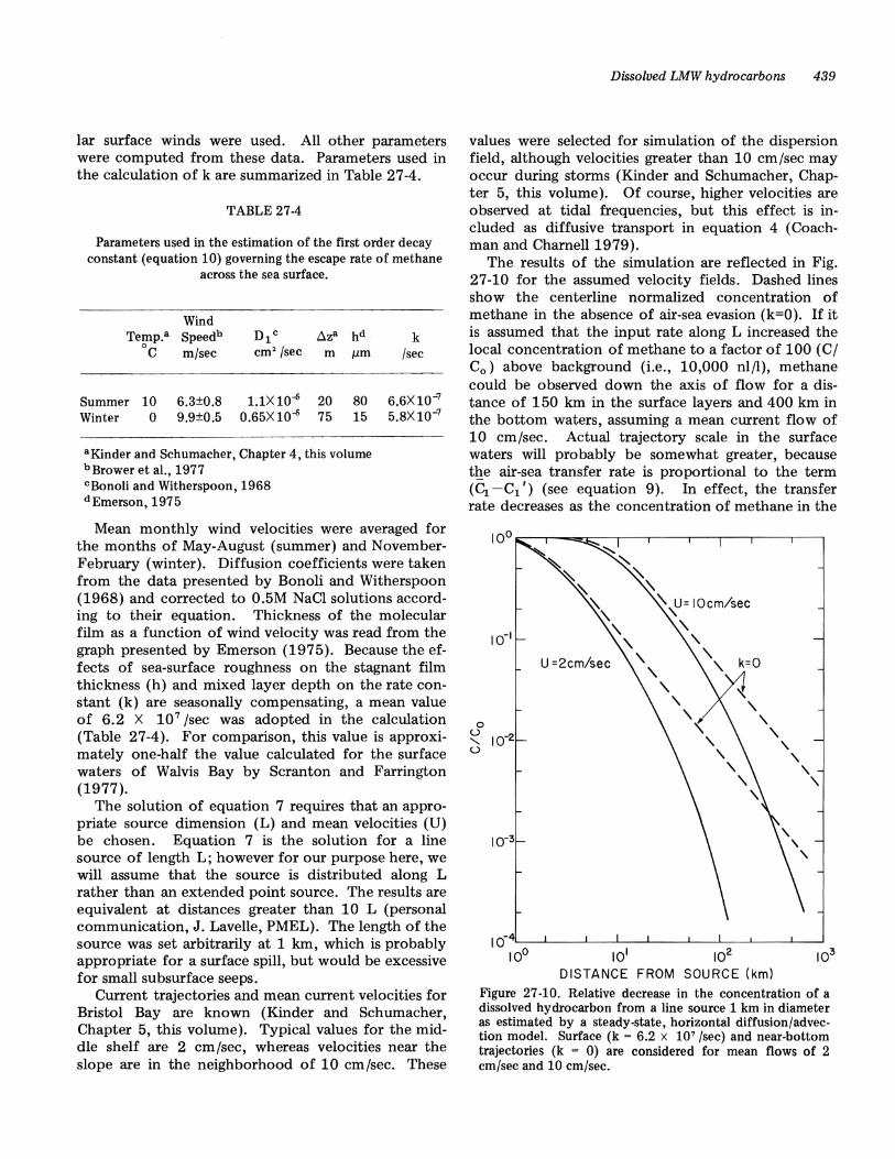
Figure 27-10. Relative decrease in the concentration of adissolved hydrocarbon from a line source 1 km in diameteras estimated by a steady-state, horizontal diffusion/advec­tion model. Surface (k = 6.2 x 10' /sec) and near-bottomtrajectories (k = 0) are considered for mean flows of 2em/sec and 10 em/sec.

values were selected fo.r simulation of the dispersionfield, although velocities greater than 10 cm/sec mayoccur during storms (Kinder and Schumacher, Chap­ter 5, this volume). Of course, higher velocities areobserved at tidal frequencies, but this effect is in­cluded as diffusive transport in equation 4 (Coach­man and Charnell1979).

The results of the simulation are reflected in Fig.27-10 for the assumed velocity fields. Dashed linesshow the centerline normalized concentration ofmethane in the absence of air-sea evasion (k=O). If itis assumed that the input rate along L increased thelocal concentration of methane to a factor of 100 (C/Co) above background (Le., 10,000 nl/l), methanecould be observed down the axis of flow for a dis­tance of 150 km in the surface layers and 400 km inthe bottom waters, assuming a mean current flow of10 cm/sec. Actual trajectory scale in the surfacewaters will probably be somewhat greater, becausethe air-sea transfer rate is proportional to the term(c; -C1 ') (see equation 9). In effect, the transferrate decreases as the concentration of methane in the

k/sec

6.6X 10-7

5.8X 10-78015

1.lX 10-6 200.65X 10-5 75

6.3±0.89.9±0.5

WindTemp.a Speedb

DC m/sec

Summer 10Winter 0

lar surface winds were used. All other parameterswere computed from these data. Parameters used inthe calculation of k are summarized in Table 27-4.

aKinder and Schumacher, Chapter 4, this volumebBrower et aI., 1977CBonoli and Witherspoon, 1968d Emerson, 1975

Mean monthly wind velocities were averaged forthe months of May-August (summer) and November­February (winter). Diffusion coefficients were takenfrom the data presented by Bonoli and Witherspoon(1968) and corrected to 0.5M NaCI solutions accord­ing to their equation. Thickness of the molecularfilm as a function of wind velocity was read from thegraph presented by Emerson (1975). Because the ef­fects of sea-surface roughness on the stagnant filmthickness (h) and mixed layer depth on the rate con­stant (k) are seasonally compensating, a mean valueof 6.2 X 107 /sec was adopted in the calculation(Table 27-4). For comparison, this value is approxi­mately one-half the value calculated for the surfacewaters of Walvis Bay by Scranton and Farrington(1977).

The solution of equation 7 requires that an appro­priate source dimension (L) and mean velocities (U)be chosen. Equation 7 is the solution for a linesource of length L; however for our purpose here, wewill assume that the source is distributed along Lrather than an extended point source. The results areequivalent at distances greater than 10 L (personalcommunication, J. Lavelle, PMEL). The length of thesource was set arbitrarily at 1 km, which is probablyappropriate for a surface spill, but would be excessivefor small subsurface seeps.

Current trajectories and mean current velocities forBristol Bay are known (Kinder and Schumacher,Chapter 5, this volume). Typical values for the mid­dle shelf are 2 cm/sec, whereas velocities near theslope are in the neighborhood of 10 cm/sec. These

440 Chemical oceanography

plume approaches the saturation value; in this casethe equilibrium concentration would be approxi­mately 50 nl/!. At reduced mean current velocities,lateral diffusion becomes more important, reducingthe concentration of methane along the axis of theplume. At velocities of only 2 cm/sec, methanewould be observable along the centerline of theplume for distances of 40 km and 80 km, dependingon whether the injection was at the surface or atdepth (k = 0). Clearly, small seeps can be traced forconsiderable distances, particularly if the injectionoccurs at depth, where hydrostatic pressure increasesthe local concentration.

At this point, it becomes pertinent to ask whathydrocarbon enrichment might be expected from agas seep, natural or otherwise. A typical wet gas, asdescribed earlier (Fig. 27-9), might be expected tocontain mole fractions of methane, ethane, and pro­pane of 0.80, 0.075, and 0.033 respectively. As­suming that the injection of a gas of this compositionoccurred at 50 m (ca. 5 atm hydrostatic pressure)and that the water column became saturated locallywith respect to each of these gases, concentrations ofmethane, ethane, and propane would reach saturationvalues of 1.8 X 108 nl/l, 2.5 X 10 7 nl/l, and 1.0 X107 nljl, respectively. (It has been assumed that theeffect of hydrostatic pressure on solubility is linear.)Assuming ambient levels of methane, ethane, andpropane of 200 nl/l, 2 nljl, and 1 nl/l (these values areabout twice the actual mean values for the middleshelf region; see Table 27-1), the enrichment factorsfor methane, ethane, and propane become 1.0 X 106

,

1.2 X 107, and 1.0 X 107

, respectively. Assumingthat the injection of gas was at 50 m as above, thesehydrocarbons would be observable along the axis ofthe plume for distances up to 1,000 km. Here asignal-to-noise ratio of approximately two is assumed.Actual longitudinal trajectories will depend on a num­ber of factors: the scale of the seep, mean currentvelocities, diffusivity near the source, and biologicaloxidation processes in the water and at the surfaceof the sediments. Biological oxidation is likely to bemuch more important at the higher concentrations ofhydrocarbons, thereby reducing the trajectory scale.Even in the surface layer, we estimate that LMW hy­drocarbons could be traced for several hundreds ofkilometers, depending on a number of factors.Among these are the state of the surface microlayer(wind velocity, surface organics, etc.), depth of themixed layer (vertical dilution), microbial oxidation,and the mean current velocity.

While the above calculations are crude, they never­theless serve to delineate the usefulness of LMWhydrocarbons as effective tracers over moderate space

scales. In the Norton Sound gas seep (Cline andHolmes 1977), the ethane plume was observable forat least 140 km downstream of the source for asource enrichment of about 20 above ambient. Re­ferring to Fig. 27-10, and assuming a 2 cm/sec meancurrent velocity near the bottom (Muench et aI.,Chapter 6, this volume), the model predicts a longi­tudinal trajectory scale of 100 km (k=O). In this case,the model appears to underestimate the actual ob­served scale, possibly by as much as a factor of two.The reasons for the disparity are numerous; amongthem are variable gas seepage rate, fluctuating cur­rents, inappropriate near-source diffusive scale, andpoor characterization of the dimension of the ethanesource. Given the hydrographic uncertainties andmodel assumptions, the prediction is probably asgood as can be developed at this time.

SUMMARY

The concentrations of dissolved LMW hydrocar­bons in Bristol Bay are relatively low when comparedwith other Alaskan shelf waters. Methane, the mostabundant hydrocarbon, is near saturation concentra­tion in surface waters, but increases significantly nearlagoons along the Alaska Peninsula. There appears tobe no major production of methane from the bottomsediments of the middle shelf but significant amountsare produced seasonally from the organic-rich sedi­ments of St. George Basin. The distribution of meth­ane is largely controlled by mean flow and frontaldynamics.

The C2+ fraction shows seasonal variability and ap­pears to be regulated by biological processes, presum­ably microorganisms. As observed elsewhere inAlaskan coastal waters, the alkenes are more abun­dant than the alkanes of the same carbon number.The concentration of ethane, for example, has a lin­ear relation to the concentration of ethene, whichsuggests a common precursor or source. Low concen­trations of LMW hydrocarbons, a relatively high[C1 ll[C2 ]+'[Ca ] ratio of 30 to 500, and a [C2 ]/

[C2 :1 ] ratio of less than 1.0, all suggest a biologicalsource. Since no evidence was found in the LMWhydrocarbon fraction for the presence of petroleum­like hydrocarbons, we conclude that Bristol Bay ispristine.

Comparison of the hydrocarbon composition oftypical natural gas and petroleum with those foundin Bristol Bay shows that small amounts of thermo­genically derived gases should be readily discerniblein the water column, depending, of course, on themagnitude of the source. On the basis of the [C1 ] /

[C2 ] +[Ca ] and [C2 ] /[C2:1 ] ratios, a thermogenic

Dissolved LMW hydrocarbons 441

REFERENCES

Bernard, B. B., J. M. Brooks, and W. M. Sackett1976 Natural gas seepage in the Gulf of

Mexico. Earth Planet. Sci. Lett. 31:48-54.

gram responding to the needs of petroleum develop­ment of the Alaskan shelf is managed by the OuterContinental Shelf Environmental Assessment Pro­gram (OCSEAP) Office.

Prudhoe Bay data are revealed atAlaska for the first time. Gas and OilJ., 57-64.

Anonymous1971

Barsdate, R. J., M. Nebert, and C. P. McRoy1974 Lagoon contributions to sediments

and water of the Bering Sea. In:Oceanography of the Bering Sea, D.W.Hood and E.J. Kelley, eds., 553-78.Inst. Mar. Sci., Occ. Pub. No.2,Univ. Alaska, Fairbanks.

field applicable to Bristol Bay can be defined. Ingeneral, [C1 ] /[C2 ] +[Ca ] ratios less than 20 and[C2 ] / [C2:1] ratios greater than 100 strongly suggesta thermogenic source. A very dry natural gas (CH4 >98 mole percent), similar to that currently being pro­duced in Cook Inlet, represents an exception to theforegoing generalizations. In all likelihood, a meth­ane-rich gas of thermogenic origin would appearto be of biological origin in the [C1 ] /[C2 ] +[Ca ] and[C2 ] /[C2 :1 ] compositional fields.

Finally, an estimate was made of the possible dis­persion scale of LMW hydrocarbons arising from aline source, using a steady-state two-dimensionalmodel. On the basis of typical mean velocities of 2and 10 em/sec with the inclusion of a sink term forair-sea exchange, it was estimated that dissolved LMWhydrocarbons would be identifiable in surface watersover distances of 40-150 km, assuming a local hydro­carbon concentration of 100:1 above ambient. Atdepth below a strong pycnocline, the horizontalmixing scale increases to 100-500 km. Actual trajec­tory scales expected in Bristol Bay will depend on anumber of factors. Among them are the strength ofthe source, degree of solution, diffusive mixing scales,air-sea exchange, and biological oxidation rates.

In this report the usefulness of LMW hydrocarbonsas a diagnostic indicator of petroleum hydrocarbon isdescribed. Not only are these gases excellent tracersof dissolved or emulsified petroleum hydrocarbons,but their ease of measurement allows real-time obser­vations to be made-a valuable adjunct to a moni­toring program.

ACKNOWLEDGMENTS

I wish to thank Lee Ohler, Anthony Young, andSusan Hamilton, who participated in the cruises tothe Bering Sea. Special thanks are due to CharlesKatz, who diligently scrutinized the data for errorsand organized it into a usable form. Criticism of themanuscript was provided by Drs. H. Curl, R. Feely,J. Lavelle, and J. Schumacher of PMEL/NOAA, Dr.K. Kvenvolden of USGS, and Dr. R. Gammon of theUniversity of Washington. To all these people I amgrateful for their helpful suggestions. Finally, I wishto express gratitude to the captains and crews of theNOAA research ships Discoverer and R/V MoanaWave, without whose assistance in the field this workcould not have been carried out.

This study, Contribution No. 456 from the NOAA/ERL Pacific Marine Laboratory, was supported bythe Bureau of Land Management through interagencyagreement with the National Oceanic and Atmos­pheric Administration, under which a multiyear pro-

1978 Light hydrocarbons in recent Texascontinental shelf and slope sediments.J. Geophys. Res. 83: 4053-61.

Bonoli, L., and P. A. Witherspoon1968 Diffusion of paraffin, cycloparaffin

and aromatic hydrocarbons in waterand some effects of salt concentra­tion. In: Advances in organic chem­istry, P.A. Schenck and I. Havenaar,eds., 373-84. Pergamon Press, NewYork.

Broecker, W. S., and T. H. Peng1974 Gas exchange rates between air and

sea. Tellus 26: 21-35.

Brooks, J. M., J. R. Gormly, and W. M. Sackett1974 Molecular and isotopic composition of

two seep gases from the Gulf of Mexi­co. Geophys. Res. Lett. 1: 213-16.

442 Chemical oceanography

Brooks, J. M., and W. M. Sackett1973 Sources, sinks, and concentrations of

light hydrocarbons in the Gulf ofMexico. J. Geophys. Res. 78: 5124­58.

1977 Significance of low-molecular-weighthydrocarbons in marine waters. In:Proc. 7th Inter. Meeting on OrganicGeochemistry. 455-68.

Brower, W. A., Jr., H. W. Searby, J. L. Wise, H. F.Diaz, and A. S. Prechtel

1977 Climatic atlas of the outer continentalshelf waters and coastal regions ofAlaska: II, Bering Sea. AEIDC, Univ.Alaska, Anchorage.

Cline, J. D., and M. L. Holmes1977 Submarine seepage of natural gas in

Norton Sound, Alaska. Science 198:1149-53.

Coachman, L. K., and R. L. Charnell1977 Finestructure in outer Bristol Bay,

Alaska. Deep-Sea Res. 24: 869-89.

1979 On lateral water mass interaction-Acase study, Bristol Bay, Alaska. J.Phys. Oceanogr. 9: 278-97.

Csanady, G. T.1973 Turbulent diffusion in the environ­

ment. D. Reidel Publishing, Boston.

Cline, J.D.1977

Dunlap, H. F., J. S. Bradley, and T. F. Moore1960 Marine seep detection-A new recon­

naissance exploration method. Geo­physics 25:275-82.

Frank, D. J., W. M. Sackett, R. Hall, and A. D. Fred­ericks

1970 Methane, ethane, and propane concen­trations in the Gulf of Mexico. Amer.Assoc. Petrol. Geol. Bull. 54: 1933-8.

DOl/DOC (Department of the Interior /Departmentof Commerce)

1975 Environmental assessment of the Gulfof Alaska, Southeastern Bering andBeaufort Seas, Boulder, Colo.

Gas exchange rates in small CanadianShield lakes. Limnol. Oceanogr. 20:754-61.

The atmospheric cycle of methane.Tellus 26: 58-70.

Emerson, S.1975

Feely, R., and J. D. Cline1977 The distribution, composition, and

transport of suspended particulatematter in the northeastern Gulf ofAlaska, southeastern Bering shelf, andlower Cook Inlet. In: Environ­mental assessment of the Alaskancontinental shelf, 8: 89-179, DOC/NOAA.

Ehhalt, D. H.1974

Carlisle, C. T., G. S. Bayliss, and D. G. Vandelinder1975 Distribution of light hydrocarbons in

seafloor sediments: Correlationsbetween geochemistry, seismic struc­ture, and possible reservoired oil andgas. OTC 2341: 65-8.

Clark, R. C., and D. W. Brown1977 Petroleum: Properties and analyses in

biotic and abiotic systems. In:Effects of petroleum on Arctic andSubarctic marine environments andorganisms, 1-90. Academic Press,N.Y.

Distribution of light hydrocarbons,C1 -C4 , in the northeast Gulf ofAlaska, Lower Cook Inlet, southeast­ern Chukchi Sea. In: Environmentalassessment of the Alaskan conti­nental shelf, 8: 180-268. DOC/NOAA.

Cline, J. D., and R. Feely1976 Distribution of light hydrocarbons,

C1 -C4 , in the Gulf of Alaska andsoutheastern Bering Shelf. In: En­vironmental assessment of the Alas­kan continental shelf, 9: 443-547.DOC/NOAA.

Cline, J. D., R. Feely, and A. Young1978 Identification of natural and anthro­

pogenic petroleum sources in theAlaskan shelf areas utilizing lowmolecular weight hydrocarbons. In:Environmental assessment of theAlaskan continental shelf, 8: 73-198,DOC/NOAA.

Harrison, H., J. E. Johnson, and J. D. Cline1980 Light hydrocarbons in the atmospher­

ic boundary layer over the NorthPacific. (Submitted to J. Geophys.Res.)

Dissolved LMW hydrocarbons 443

Moore, B. J., R. D. Miller, and R. D. Schrewsbury1966 Analyses of natural gases of the

United States, 1964. Bureau ofMines IC-8302: 1-144.

Nikonov, V. F.1972 Distribution of methane homologs in

gas and oil fields. Doklady Akad.Nauk SSSR 226: 234-6.

Hunt, J. M.1974 Hydrochemistry of Black Sea. In:

The Black Sea, geology, chemistry,and biology, E.T. Degens and D.A.Ross, eds., 499-504. Amer. Assoc.Petrol.Geol. Mem. 20.

Okubo, A.1971 Oceanic diffusion diagrams.

Sea Res. 18: 789-802.Deep-

Kelly, T. E.1968

Kinder, T. H.1977

Gas accumulations in non-marinestrata, Cook Inlet, Basin, Alaska. In:Natural gases of North America, B.W.Beebe, ed., 49-64. Amer. Assoc.Petrol. Geol. Mem. 9, Part I.

The hydrographic structure over thecontinental shelf near Bristol Bay,Alaska, June 1976. Dep. Oceanogr.Tech. Rep. M77-3: 1-61. Univ. ofWashington.

Oremland, R. S.1975 Methane production in shallow-water,

tropical marine sediments. Appl.Microbiol. 30: 602-8.

Reeburgh, W. S., and D. T. Heggie1977 Microbial methane consumption reac­

tions and their effect on methanedistributions in freshwater and marineenvironments. Limnol. Oceanogr. 22:1-9.

Kinder, T. H., and L. K. Coachman1978 The front overlying the continental

slope in the eastern Bering Sea. J.Geophys. Res. 83: 4551-9.

Kvenvolden, K. A., K. Weliby, C. H. Nelson, and D. J.Desmarais

1979 Submarine carbon dioxide seep inNorton Sound, Alaska. Science 205:1264-6.

Sackett, W. M.1977 Use of hydrocarbon sniffing in off-

shore exploration. J. Geochem.Explor.7: 243-54.

Schumacher, J. D., T. H. Kinder, D. H. Pashinski, andR. L. Charnell

1979 A structural front over the continentalshelf of the eastern Bering Sea. J.Phys. Oceanogr. 9: 79-87.

Scranton, M. I., and J. W. Farrington1977 Methane production in the waters

off Walvis Bay. J. Geophys. Res.82: 4947-53.

Scranton, M. I., and P. G. Brewer1977 Occurrence of methane in the near

surface waters of the western subtrop­ical North Atlantic. Deep-Sea Res.24: 127-38.

Lamontagne, R. A., W. D. Smith, and J. W. Swinner­ton

1975 C1 -Ca hydrocarbons and chlorophylla concentrations in the equatorialPacific Ocean. In: Analytical methodsin oceanography, T.R.P. Gibbs, Jr.,ed., 163-71. Advances in ChemistrySeries 147, Amer. Chern. Soc.

McCarty, P. L.1964 The methane fermentation. In:

Principles and applications in aquaticmicrobiology, H. Heukelekian andN.C. Dondero, eds., 314-43. JohnWiley, N. Y.

Sharma, G. D.1979 The Alaskan shelf.

N. Y.Springer-Verlag,

444 Chemical oceanography

Smith, A. M., and R. J. Cook1974 Implications of ethylene production

by bacteria for biological balance ofsoil. Nature (London) 252: 703-5.

Swinnerton, J. W., and R. A. Lamontagne1974 Oceanic distribution of low-molecular­

weight hydrocarbons. Environ. Sci.and Techno!. 8: 657-63.

Wilson, D. F., J. W. Swinnerton, and R. A. Lamon­tagne

1970 Production of carbon monoxide andgaseous hydrocarbons in seawater:Relation to dissolved organic carbon.Sci. 168: 1577-9.

Swinnerton, J. W., R. A. Lamontagne, and J. S. Hunt1977 Field study of carbon monoxide and

light hydrocarbons production relatedto natural biological processes, NRLRep. 8099: 1-9.

Wolfe, R. S.1971 Microbial formation of methane. In:

Advances in microbial physiology,A.H. Hose and J.F. Wilkinson, eds., 6:107-46. Academic Press, N. Y.

Swinnerton, J. W., and V. J. Linnenbom1967 Determination of the C1 to C4

hydrocarbons in seawater by gaschromatography. J. Chromatogr. Sci.5: 570-3.

Yamamoto, S., J. B. Alcauskas, and T. E. Grozier1976 Solubility of methane in distilled

water and seawater. J. Chern. Eng.Data 21: 78-80.