Embed Size (px)
Citation preview
DISTRIBUTION OF NEW TEMPERATURE
EXTREMES
by
BAHTIYAR BABANAZAROV, B.S.
A THESIS
IN
MATHEMATICS
Submitted to the Graduate Faculty of Texas Tech University in
Partial Fulfillment of the Requirements for
the Degree of
MASTER OF SCIENCE
Approved
Clyde Martin Chairperson of the Committee
Akif Ibragimov
Accepted
John Borrelli Dean of the Graduate School
December, 2006
ACKNOWLEDGEMENTS
First, I would like to thank my advisor Horn Prof. Clyde Martin, who were very
understanding, supportive and inspiring to me throughout my study. He was inspiring
and helpful in all aspects of the thesis. This thesis would not happen without his
support and motivation.
I also would like to thank Prof. Akif Ibragimov for serving in the committee and
for useful discussions.
I would like to thank very special and close friend of mine who supported me
throughout my studies and always pushed me to work harder and harder. I would
also like to thank all my friends in Lubbock for their continuous and endless moral
support. Resul, Mehmet B., Mehmet K., Hakan, Abdulhadi, Emrah, Faruk, Kazim
abi. I also would like to thank some of my friends who supported me from the
distance. Thanks to Resat abi, Saim abi, Tansel abi and Murat abi.
Finally, I would like to thank my wife Gulzira for her support and dedication to
me. Now, this is the time to thank my parents. I have to thank them for almost
everything...
ii
CONTENTS
ACKNOWLEDGEMENTS . . . . . . . . . . . . . . . . . . . . . . . . . . ii
LIST OF FIGURES . . . . . . . . . . . . . . . . . . . . . . . . . . . . . . v
I INTRODUCTION . . . . . . . . . . . . . . . . . . . . . . . . . . . . 1
1.1 Global Warming . . . . . . . . . . . . . . . . . . . . . . . . . . 1
1.1.1 Causes of Global Warming . . . . . . . . . . . . . . . . . . 1
1.1.2 Complexity of the problem . . . . . . . . . . . . . . . . . . 1
1.2 Our approach to the problem . . . . . . . . . . . . . . . . . . . 2
1.2.1 What is extreme value theory and how are we applying it
to this problem? . . . . . . . . . . . . . . . . . . . . . . . . 2
1.3 Thesis Outline . . . . . . . . . . . . . . . . . . . . . . . . . . . 3
II HISTORY OF EXTREME VALUE THEORY . . . . . . . . . . . . 4
2.1 Historical Background . . . . . . . . . . . . . . . . . . . . . . . 4
2.2 Some other applications of Extreme Value Theory . . . . . . . 5
2.3 Models for Extreme Values . . . . . . . . . . . . . . . . . . . . 5
III EXTREME VALUE MODELS . . . . . . . . . . . . . . . . . . . . . 7
3.1 Classical Block Maxima Models . . . . . . . . . . . . . . . . . 7
3.1.1 Types of distributions . . . . . . . . . . . . . . . . . . . . . 8
3.1.2 Outline Proof of the Extremal Types Theorem . . . . . . . 9
3.2 Threshold Models . . . . . . . . . . . . . . . . . . . . . . . . . 11
3.2.1 The Generalized Pareto Distribution . . . . . . . . . . . . 11
3.2.2 Proof of Theorem 3.3 . . . . . . . . . . . . . . . . . . . . . 12
IV SELECTING A MODEL FOR THE PROBLEM . . . . . . . . . . . 16
4.1 Background . . . . . . . . . . . . . . . . . . . . . . . . . . . . 16
4.1.1 Filtering the data . . . . . . . . . . . . . . . . . . . . . . . 16
4.1.2 Evaluating the data using Matlab/ Matlab Part . . . . . . 16
4.1.3 Table of extreme value exceedances . . . . . . . . . . . . . 21
4.2 Picking a model . . . . . . . . . . . . . . . . . . . . . . . . . . 24
iii
4.2.1 Picking Frechet distribution type . . . . . . . . . . . . . . 25
4.3 Least squares regression of the Model . . . . . . . . . . . . . . 25
4.4 Conclusion . . . . . . . . . . . . . . . . . . . . . . . . . . . . . 28
iv
LIST OF FIGURES
4.1 Frequency of extreme exceedances . . . . . . . . . . . . . . . . . . . . 24
v
CHAPTER I
INTRODUCTION
1.1 Global Warming
1.1.1 Causes of Global Warming
Global warming is one of the very widely discussed topics in our days. It is known
as a human caused problem and the main cause is the burning of fossil fuels-coal,
oil and gas which release carbon dioxide into the atmosphere. As a consequence
atmosphere gets polluted with carbon which blankets the earth and traps in heat.
The trapped heat causes global warming. [1]
In addition to the carbon dioxide, other atmospheric greenhouse gases such as
chlorofluorocarbons and their substitutes, methane, nitrous oxide, etc. have been ob-
served to increase. It is also claimed that atmospheric carbon dioxide concentrations
have increased since the mid-1700s through fossil fuel burning and changes in land
use, with more than 80% of this increase occurring since 1900. As an example, only
electricity generation itself causes 37% of global CO2 emissions. [2]
1.1.2 Complexity of the problem
Although the research show the causes of the global warming, it is not an easy
task to calculate or answer some problems such as
• exactly how fast global warming is happening
• exactly how much it will change
• what part of the earth will be affected more
[3]
The complexity of this is due to the complexity of atmospheric system that we
live in. It is too complicated to be explained with a few causes and predictions.
On the other hand, there are some predictions about which scientists are confident.
According to these mid-continent warming will be greater than over the oceans, and
1
there will be greater warming at higher latitudes. Some polar and glacial ice will
melt, and the oceans will warm; both effects will contribute to higher sea levels. The
hydrologic cycle will change and intensify, leading to changes in water supply as well
as flood and drought patterns. There will be considerable regional variations in the
resulting impacts. [3]
1.2 Our approach to the problem
As we mentioned above, global warming is multi-parametered complex problem
where we have to consider multiple parameters including but not limited to the tem-
perature increase/decrease, greenhouse gases’ change in the atmosphere, human ac-
tivities that might possibly affect the balance in the nature etc.
This thesis, naturally with its size and scope, is far away from considering all those
parameters and does not claim to prove/disprove the global warming. We are mainly
focused on how the extreme weather temperatures are distributed between 1913 and
1964, and what kind of statistical inferences we can make by using the statistical
method called extreme value theory.
1.2.1 What is extreme value theory and how are we applying it to this problem?
We will answer this question first by giving the historical background. Then,
we will see in detail the main types of extreme value models with their properties.
Following these steps, we go to the main part of the thesis; picking the appropriate
extreme value model to our approach and analyze it. Here, we will seek for the
answer to our one of the main questions: Is the frequency of extreme values are
increasing or decreasing? The answer to this question will actually be the main
part of the conclusion.
2
1.3 Thesis Outline
Here is the brief outline of the thesis:
In Chapter 2, we discuss the historical background of the extreme value theory
with major application examples.
In Chapter 3, we see the three types of models that extreme values have and
explore the properties of them in detail.
In Chapter 4, we discuss which model we use and why we use it.
Finally, we conclude the thesis and explain the results.
3
CHAPTER II
HISTORY OF EXTREME VALUE THEORY
2.1 Historical Background
Unlike most statistical methods which mainly deal with what goes on in the center
of a statistical distribution, Extreme Value Theory concerned more with what happens
in the extreme ends. Since by their nature, extreme events occur rarely, here we do
not have a comfort of having many observations, at least in the most cases. This
requires us to be able to guess more often than estimate by calculation as we would
do in a most statistical methods. So, Extreme Value Theory is a collection of methods
that deal with extreme or rare events. [4]
Emil Julius Gumbel, a German mathematician is considered to be the founder of
the extreme value theory. He once said ”It seems that the rivers know the theory. It
only remains to convince the engineers of the validity of this analysis.” [4]. He devel-
oped a distribution type, called Gumbel distribution which is used to find the sample
maximum (or the minimum) of a number of various distributions. The distributions
of the samples could be of the normal or exponential type. As we can see from the
quote of Gumbel, historically his original focus was to predict the maximum level of
the river.
Theorem called three types theorem is the cornerstone of the extreme value theory.
It was first stated by Fisher and Tipett [4] and was proved rigorously by Gnedenko to
the effect that there are only three types of distributions which can arise as limiting
distributions of extremes in random samples. [4]
Gumbel followed this theory and developed statistical methodology for extreme
values based on fitting the extreme value distributions to data consisting of maxima or
minima over a fixed time intervals. [4] To see an example, consider applying Gumbel’s
method to the annual maxima of a series of river flows for a certain period time. Now,
let’s say you want to find the maximum level of a river in a particular year having had
the list of maximum values for the past fifty years. Gumbel distribution is employed
4
to find the maximum and then this information is used to predict the probability of
maximums that might occur in the future. Therefore, predicting this would help you
to determine how tall should an embankment be so you do not get a flood.
2.2 Some other applications of Extreme Value Theory
Application of Extreme Value Theory (EVT) is not limited to the natural phe-
nomenon as once it was when Gumbel started this method. Recently, insurance and
finance world have been using the EVT very intensively. In insurance, a typical prob-
lem would be pricing of the catastrophic loss. EVT would be used to predict this.
In financial environment the example of main application of EVT is to stock market.
For example, what is the probability of stock market crash in 3 days? In addition to
the stock market, EVT is widely used in industry to calculate the industry losses. [5]
Another area where EVT is intensively used is risk-management. An example in
this field would be credit risk management. Expected loss, unexpected loss and stress
loss are the main parameters in this area that people try to estimate by using the
EVT. [5]
Gumbel and similar type distributions are therefore used in extreme value theory.
We will discuss all the details of the EVT such as what distribution families are there,
what models we have etc. in the coming chapter.
Properties of the Gumbel distribution:
• The standard Gumbel distribution has µ = 0 and β = 1
• cumulative distribution function F (x) = exp{− exp(−x)}
• and probability density function f(x) = exp{−x} ∗ exp{− exp(−x)}
2.3 Models for Extreme Values
We should note here briefly that there are mainly two types of models for Extreme
Values. We will just state them here briefly and discuss them detailly in the next
chapter.
5

1. Block Maxima
2. Threshold Models
We should note here that in recent years, the methodology that was once used by
Gumble has shifted towards the methods based on the exceedances over thresholds
rather than annual maxima. The limiting distribution in this context leads to the
distribution type called Pareto distribution. [6]
There are two main reason why threshold methods preferred to annual maximum
methods:
• The data is used more efficiently by taking all exceedances over a certain thresh-
old
• It is easily extended to situations where one wants to study how the extreme
levels of one variable, Y depends on some other variable, X
This completes the discussion of the historical background and main types of
models for Extreme Values. In the next chapter we will see the properties of these
distribution families and types in great detail.
6
CHAPTER III
EXTREME VALUE MODELS
Analysis of extreme events or extreme values requires estimation of the proba-
bilities of extreme events. Extreme value models are developed using asymptotic
arguments.
There are two families of models that describe the Extreme Values. First one is
the classical Block Maxima family models and the other one is Threshold Models
or Peak Over Threshold Models. [6] Threshold models have been developed lately
and have certain advantages over the Block Maxima models. The main advantage in
Threshold Model is the data is used more efficiently by taking all exceedances over
a certain threshold whereas in the Block Maxima model, you might waste the data
if one block happens to contain more extreme events than another. [4] Although,
it seems like they are two different families of models, in the later sections of this
chapter we will show that one family has a corresponding distribution family within
the another one.
3.1 Classical Block Maxima Models
Suppose
X1...Xn
are independent random variables with common distribution F.
F (x) = Pr(Xj ≤ x)∀j, x
The distribution function of the maximum
Mn = max{X1...Xn}
is given by the F n:
{Pr(Mn ≤ x)} = Pr{X1 ≤ x,X2 ≤ x, ...., Xn ≤ x}
7
= Pr{X1 ≤ x} ∗ Pr{X2 ≤ x}.... ∗ Pr{Xn ≤ x}
= F n(x)
[4]
This does not give us anything useful except we know that this distribution → 0
as n →∞ when it is in the range of 0 and 1. [4]
It turns out that we get a useful result by renormalizing. Define scaling constants
an ≥ 0 and bn so that
Pr{Mn − bn
an
≤ x} = Pr{Mn ≤ an ∗ x + bn}
= F n(an ∗ x + bn)
→ H(x) as n →∞ where H is nondegenerate. [6, p. 45] In another words,
Pr{Mn−bn
an≤ x} → H(x) as n →∞
It is beyond the scope of this thesis to discuss how to determine the constants an
and bn, but the examples will be provided for different an’s and bn’s where they will
lead to different types of Extreme Value Models.
3.1.1 Types of distributions
Theorem 3.1 [6, p. 48] If there exist sequence of constants {an} and {bn} such
that
Pr{Mn−bn
an≤ z} → G(z) as n → ∞,
where G is a non-degenerate distribution function, then G belongs to one of the
following families:
1. G(z) = Gumbel type:
• G(z) = exp{−exp(−( z−aa
))} where -∞ < z < ∞
2. G(z) = Frechet type:
8
• G(z) = 0 , if z ≤ b
• G(z) = exp{−( z−ba
)−α}, if z > b
3. Weibull type:
• G(z) = exp{−(−( z−aa
)α)}, if z < b
• G(z) = 1 , if z ≥ b
Each family has a location and scale parameter, b and a respectively; additionally,
Frechet and Weibull families have a shape parameter α. The importance of this
theorem is given any F, its limit distribution is one of the above families. It is kind
of equivalence of central limit theorem in extreme values.
These three distributions can be combined into a single family of models having
distribution functions of the form
G(z) = exp{−(1 + ξ ∗ (z − µ
σ))−1/ξ} (3.1)
This is called generalized extreme value(GEV) family of distributions. Now The-
orem 3.1 can be interpreted as if there exist sequences of constants {an} and {bn}such that
Pr{Mn−bn
an≤ z} → G(z) as n → ∞,
where G is a non-degenerate function, then G is the a member of the GEV family.
3.1.2 Outline Proof of the Extremal Types Theorem
Here is the informal proof: [6, p.49-51]
Formal justification of the extremal theorem is technical, though not especially
complicated - see Leadbetter et al. (1983), for example. In this section we give
informal proof. First, it is convenient to make the following definition.
Definition 3.1 A distribution G is said to be max-stable if, for every n = 2, 3, ...,
there are constants αn > 0 and βn such that Gn(αnz + βn) = G(z).
9
Since Gn is the distribution function of Mn = max{X1, ..., Xn}, where the Xi are
independent variables each having distribution function G, max-stability is a property
satisfied by distributions for which the operation of taking samle maxima leads to an
identical distribution, apart from a change of scale and location. The connection with
the extreme value limit laws is made by the following result.
Theorem 3.2 A distribution is max-stable if, and only if, it is a generalized value
distribution.
It requires only simple algebra to check that all members of the GEV family are
indeed max-stable. The converse requires ideas from functional analysis that are
beyond the scope of this book.
Theorem 3.2 is used directly in the proof of the extremal types theorem. The idea
is to consider Mnk, the maximum random variable in a sequence of nxk variables for
some large value of n. This can be regarded as the maximum of a single sequence
of length nxk, or as the maximum of k maxima, each of which is the maximum of
n observations. More precisely, suppose the limit distribution of Mn−bn
anis G. So, for
large enough n,
Pr{(Mn − bn
an
) ≤ z} ≈ G(z)
By Theorem 3.1. Hence, for any integer k, since nk is large,
Pr{(Mnk − bnk
ank
) ≤ z} ≈ G(z) (3.2)
But, since Mnk is the maximum of k variables having the same distribution as
Mn,
Pr{(Mnk − bnk
ank
) ≤ z} = (Pr{(Mn − bn
an
) ≤ z})k (3.3)
Hence, by (3.2) and (3.3) respectively,
Pr{Mnk ≤ z} ≈ G(z − bnk
ank
)
10
and
Pr{Mnk ≤ z} ≈ Gk(z − bn
an
)
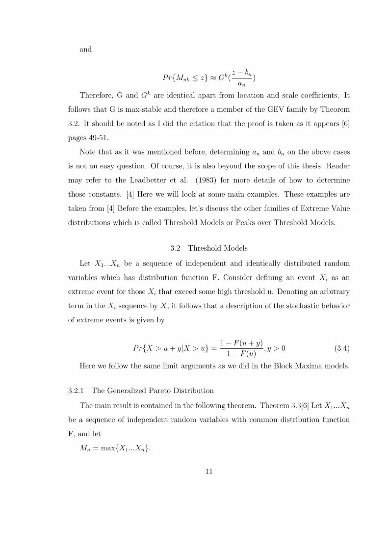
Therefore, G and Gk are identical apart from location and scale coefficients. It
follows that G is max-stable and therefore a member of the GEV family by Theorem
3.2. It should be noted as I did the citation that the proof is taken as it appears [6]
pages 49-51.
Note that as it was mentioned before, determining an and bn on the above cases
is not an easy question. Of course, it is also beyond the scope of this thesis. Reader
may refer to the Leadbetter et al. (1983) for more details of how to determine
those constants. [4] Here we will look at some main examples. These examples are
taken from [4] Before the examples, let’s discuss the other families of Extreme Value
distributions which is called Threshold Models or Peaks over Threshold Models.
3.2 Threshold Models
Let X1...Xn be a sequence of independent and identically distributed random
variables which has distribution function F. Consider defining an event Xi as an
extreme event for those Xi that exceed some high threshold u. Denoting an arbitrary
term in the Xi sequence by X, it follows that a description of the stochastic behavior
of extreme events is given by
Pr{X > u + y|X > u} =1− F (u + y)
1− F (u), y > 0 (3.4)
Here we follow the same limit arguments as we did in the Block Maxima models.
3.2.1 The Generalized Pareto Distribution
The main result is contained in the following theorem. Theorem 3.3[6] Let X1...Xn
be a sequence of independent random variables with common distribution function
F, and let
Mn = max{X1...Xn}.
11
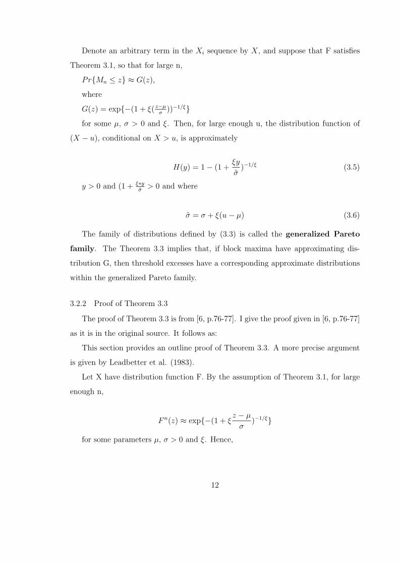
Denote an arbitrary term in the Xi sequence by X, and suppose that F satisfies
Theorem 3.1, so that for large n,
Pr{Mn ≤ z} ≈ G(z),
where
G(z) = exp{−(1 + ξ( z−µσ
))−1/ξ}for some µ, σ > 0 and ξ. Then, for large enough u, the distribution function of
(X − u), conditional on X > u, is approximately
H(y) = 1− (1 +ξy
σ)−1/ξ (3.5)
y > 0 and (1 + ξ∗yσ
> 0 and where
σ = σ + ξ(u− µ) (3.6)
The family of distributions defined by (3.3) is called the generalized Pareto
family. The Theorem 3.3 implies that, if block maxima have approximating dis-
tribution G, then threshold excesses have a corresponding approximate distributions
within the generalized Pareto family.
3.2.2 Proof of Theorem 3.3
The proof of Theorem 3.3 is from [6, p.76-77]. I give the proof given in [6, p.76-77]
as it is in the original source. It follows as:
This section provides an outline proof of Theorem 3.3. A more precise argument
is given by Leadbetter et al. (1983).
Let X have distribution function F. By the assumption of Theorem 3.1, for large
enough n,
F n(z) ≈ exp{−(1 + ξz − µ
σ)−1/ξ}
for some parameters µ, σ > 0 and ξ. Hence,
12
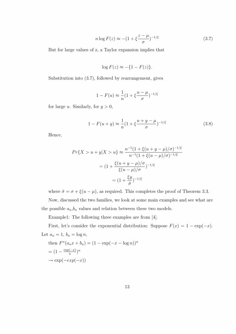
n log F (z) ≈ −(1 + ξz − µ
σ)−1/ξ (3.7)
But for large values of z, a Taylor expansion implies that
log F (z) ≈ −{1− F (z)}.
Substitution into (3.7), followed by rearrangement, gives
1− F (u) ≈ 1
n(1 + ξ
u− µ
σ)−1/ξ
for large u. Similarly, for y > 0,
1− F (u + y) ≈ 1
n(1 + ξ
u + y − µ
σ)−1/ξ (3.8)
Hence,
Pr{X > u + y|X > u} ≈ n−1(1 + ξ(u + y − µ)/σ)−1/ξ
n−1(1 + ξ(u− µ)/σ)−1/ξ
= (1 +ξ(u + y − µ)/σ
ξ(u− µ)/σ)−1/ξ
= (1 +ξy
σ)−1/ξ
where σ = σ + ξ(u− µ), as required. This completes the proof of Theorem 3.3.
Now, discussed the two families, we look at some main examples and see what are
the possible an,bn values and relation between these two models.
Example1: The following three examples are from [4].
First, let’s consider the exponential distribution: Suppose F (x) = 1 − exp(−x).
Let an = 1, bn = log n,
then F n(anx + bn) = (1− exp(−x− log n))n
= (1− exp(−x)n
)n
→ exp(−exp(−x))
13
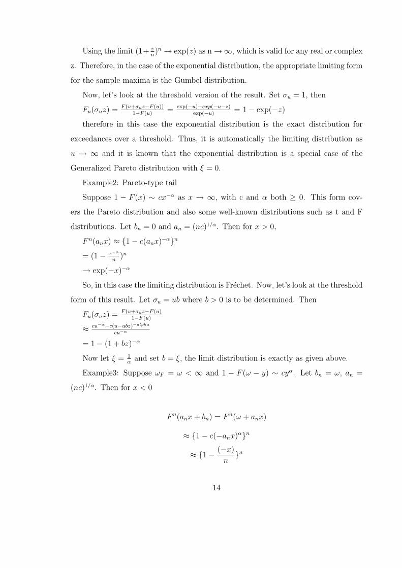
Using the limit (1+ zn)n → exp(z) as n→∞, which is valid for any real or complex
z. Therefore, in the case of the exponential distribution, the appropriate limiting form
for the sample maxima is the Gumbel distribution.
Now, let’s look at the threshold version of the result. Set σu = 1, then
Fu(σuz) = F (u+σuz−F (u))1−F (u)
= exp(−u)−exp(−u−z)exp(−u)
= 1− exp(−z)
therefore in this case the exponential distribution is the exact distribution for
exceedances over a threshold. Thus, it is automatically the limiting distribution as
u → ∞ and it is known that the exponential distribution is a special case of the
Generalized Pareto distribution with ξ = 0.
Example2: Pareto-type tail
Suppose 1 − F (x) ∼ cx−α as x → ∞, with c and α both ≥ 0. This form cov-
ers the Pareto distribution and also some well-known distributions such as t and F
distributions. Let bn = 0 and an = (nc)1/α. Then for x > 0,
F n(anx) ≈ {1− c(anx)−α}n
= (1− x−α
n)n
→ exp(−x)−α
So, in this case the limiting distribution is Frechet. Now, let’s look at the threshold
form of this result. Let σu = ub where b > 0 is to be determined. Then
Fu(σuz) = F (u+σuz−F (u)1−F (u)
≈ cu−α−c(u−ubz)−alpha
cu−α
= 1− (1 + bz)−α
Now let ξ = 1α
and set b = ξ, the limit distribution is exactly as given above.
Example3: Suppose ωF = ω < ∞ and 1 − F (ω − y) ∼ cyα. Let bn = ω, an =
(nc)1/α. Then for x < 0
F n(anx + bn) = F n(ω + anx)
≈ {1− c(−anx)α}n
≈ {1− (−x)
n}n
14
→ exp{−(−x)α}
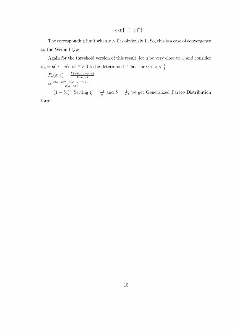
The corresponding limit when x > 0 is obviously 1. So, this is a case of convergence
to the Weibull type.
Again for the threshold version of this result, let u be very close to ω and consider
σu = b(ω − u) for b > 0 to be determined. Then for 0 < z < 1b
Fu(σuz) = F (u+σuz−F (u)1−F (u)
≈ c(ω−u)α−c(ω−u−σuz)α
c(ω−u)α
= (1 − bz)α Setting ξ = −1α
and b = 1α, we get Generalized Pareto Distribution
form.
15
CHAPTER IV
SELECTING A MODEL FOR THE PROBLEM
4.1 Background
4.1.1 Filtering the data
This project is completely based on the data that we obtained from National
Climatic Data Center’s web site. This data is the maximum daily temperatures from
a fixed station near Lubbock between 1913 and 1964.
Originally this data was in the Microsoft Excel format. Since all the calculations
were made in Matlab, the original data was filtered and stored in an array. The reason
why we call it filtering is because when we had the data in original form, there were
some letters representing Fahrenheit(F) and some other related terms. Obviously we
could not do anything with the numbers mixed with letters, so we had to filter the
data.
4.1.2 Evaluating the data using Matlab/ Matlab Part
Stored the data into matrix in Matlab, now it is time to write some code in Matlab
to explore the data more detailly. Recall that our aim is to fit our data into one of
the extreme value models. In order to be able to do so, we need to know more about
our data such as whether extreme values are increasing/decreasing, is the relative
frequency of the extreme values are getting increased/decreased etc.
The Matlab code is heavily commented and explained thoroughly, so we just attach
the code. Here is the Matlab code which gives the extreme exceedances between 1914
and 1963.
A = [x1 x2 x3 x4 x5 x6 x7 x8 x9 x10 x11 x12 x13 x14 x15 x16
x17 x18 x19 x20 x21 x22 x23 x24 x25 x26 x27 x28 x29 x30
x31];
16
% x1 is a column vector, it is the 1st day of the each month
%between 1914 % and 1963.
% As seen above, matrix A is consists of these column vectors.
k = 1;
k2 = 1;
% This is to put whole data into one string, in case if I want
%to graph everything at once
for i = 1:599
for j = 1:31
z(k,1) = A(i,j);
k = k+1;
end
end
% putting data into one string ends here
t = 1;
n = 2;
% putting the data of 1913 into one string
for i = 1:124
y1913(i,1) = z(i,1);
end
% taking out the 1913’s data out of the general string
% because 1913 is not given as a complete year. We have
%only September through December and including 1913
%messes up the analysis
[a,b] = size(z);
17
c = 1;
for i = 125:a
z2(c,1) = z(i,1);
c = c+1;
end
%=====================================================
[a,b] = size(z2);
t = 1;
v = 5;
rown = 1;
coln = 1;
% putting the rest of the data into years t=1 means 1914,
% t=49 means 1963
while(t<50)
for i = v:v+11
for j = 1:31
B(rown,t) = A(i,j);
rown = rown+1;
end
end
rown = 1;
t = t+1;
v = v+12;
end
% end putting the data into years t=1 means 1914, t=49 means 1963
18
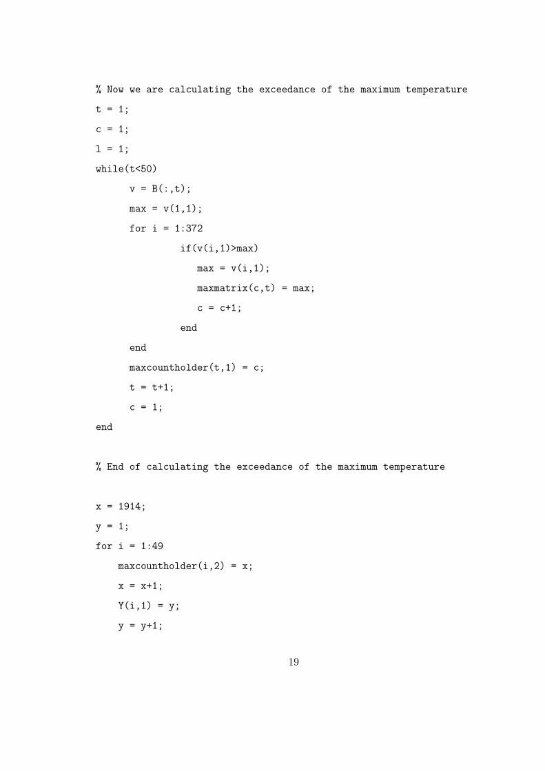
% Now we are calculating the exceedance of the maximum temperature
t = 1;
c = 1;
l = 1;
while(t<50)
v = B(:,t);
max = v(1,1);
for i = 1:372
if(v(i,1)>max)
max = v(i,1);
maxmatrix(c,t) = max;
c = c+1;
end
end
maxcountholder(t,1) = c;
t = t+1;
c = 1;
end
% End of calculating the exceedance of the maximum temperature
x = 1914;
y = 1;
for i = 1:49
maxcountholder(i,2) = x;
x = x+1;
Y(i,1) = y;
y = y+1;
19
end
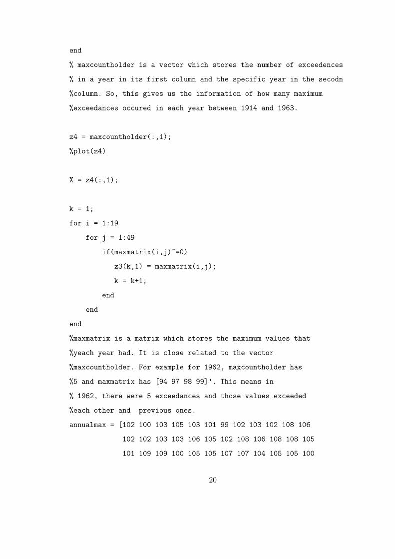
% maxcountholder is a vector which stores the number of exceedences
% in a year in its first column and the specific year in the secodn
%column. So, this gives us the information of how many maximum
%exceedances occured in each year between 1914 and 1963.
z4 = maxcountholder(:,1);
%plot(z4)
X = z4(:,1);
k = 1;
for i = 1:19
for j = 1:49
if(maxmatrix(i,j)~=0)
z3(k,1) = maxmatrix(i,j);
k = k+1;
end
end
end
%maxmatrix is a matrix which stores the maximum values that
%yeach year had. It is close related to the vector
%maxcountholder. For example for 1962, maxcountholder has
%5 and maxmatrix has [94 97 98 99]’. This means in
% 1962, there were 5 exceedances and those values exceeded
%each other and previous ones.
annualmax = [102 100 103 105 103 101 99 102 103 102 108 106
102 102 103 103 106 105 102 108 106 108 108 105
101 109 109 100 105 105 107 107 104 105 105 100
20
104 106 105 108 103 103 104 103 106 104 100 100]’;
%=========== end of the program ================================
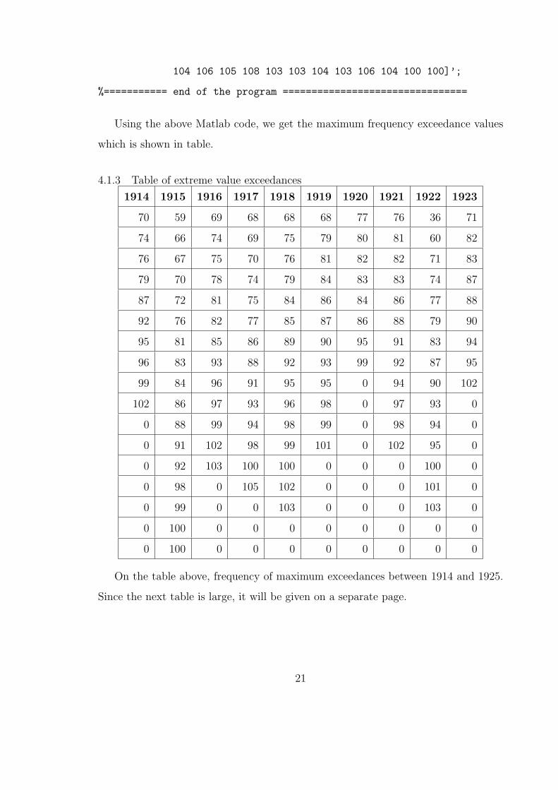
Using the above Matlab code, we get the maximum frequency exceedance values
which is shown in table.
4.1.3 Table of extreme value exceedances
1914 1915 1916 1917 1918 1919 1920 1921 1922 1923
70 59 69 68 68 68 77 76 36 71
74 66 74 69 75 79 80 81 60 82
76 67 75 70 76 81 82 82 71 83
79 70 78 74 79 84 83 83 74 87
87 72 81 75 84 86 84 86 77 88
92 76 82 77 85 87 86 88 79 90
95 81 85 86 89 90 95 91 83 94
96 83 93 88 92 93 99 92 87 95
99 84 96 91 95 95 0 94 90 102
102 86 97 93 96 98 0 97 93 0
0 88 99 94 98 99 0 98 94 0
0 91 102 98 99 101 0 102 95 0
0 92 103 100 100 0 0 0 100 0
0 98 0 105 102 0 0 0 101 0
0 99 0 0 103 0 0 0 103 0
0 100 0 0 0 0 0 0 0 0
0 100 0 0 0 0 0 0 0 0
On the table above, frequency of maximum exceedances between 1914 and 1925.
Since the next table is large, it will be given on a separate page.
21
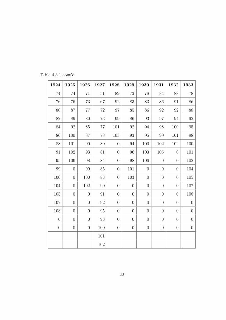
Table 4.3.1 cont’d
1924 1925 1926 1927 1928 1929 1930 1931 1932 1933
74 74 71 51 89 73 78 84 88 78
76 76 73 67 92 83 83 86 91 86
80 87 77 72 97 85 86 92 92 88
82 89 80 73 99 86 93 97 94 92
84 92 85 77 101 92 94 98 100 95
86 100 87 78 103 93 95 99 101 98
88 101 90 80 0 94 100 102 102 100
91 102 93 81 0 96 103 105 0 101
95 106 98 84 0 98 106 0 0 102
99 0 99 85 0 101 0 0 0 104
100 0 100 88 0 103 0 0 0 105
104 0 102 90 0 0 0 0 0 107
105 0 0 91 0 0 0 0 0 108
107 0 0 92 0 0 0 0 0 0
108 0 0 95 0 0 0 0 0 0
0 0 0 98 0 0 0 0 0 0
0 0 0 100 0 0 0 0 0 0
101
102
22
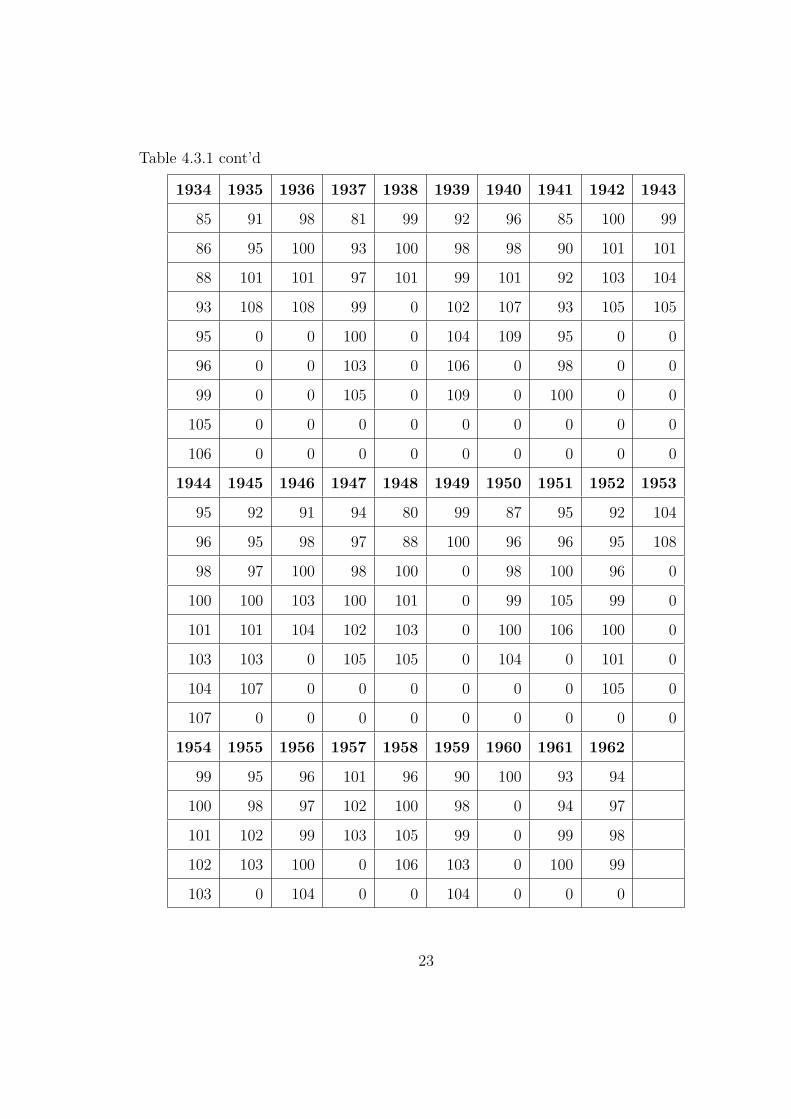
Table 4.3.1 cont’d
1934 1935 1936 1937 1938 1939 1940 1941 1942 1943
85 91 98 81 99 92 96 85 100 99
86 95 100 93 100 98 98 90 101 101
88 101 101 97 101 99 101 92 103 104
93 108 108 99 0 102 107 93 105 105
95 0 0 100 0 104 109 95 0 0
96 0 0 103 0 106 0 98 0 0
99 0 0 105 0 109 0 100 0 0
105 0 0 0 0 0 0 0 0 0
106 0 0 0 0 0 0 0 0 0
1944 1945 1946 1947 1948 1949 1950 1951 1952 1953
95 92 91 94 80 99 87 95 92 104
96 95 98 97 88 100 96 96 95 108
98 97 100 98 100 0 98 100 96 0
100 100 103 100 101 0 99 105 99 0
101 101 104 102 103 0 100 106 100 0
103 103 0 105 105 0 104 0 101 0
104 107 0 0 0 0 0 0 105 0
107 0 0 0 0 0 0 0 0 0
1954 1955 1956 1957 1958 1959 1960 1961 1962
99 95 96 101 96 90 100 93 94
100 98 97 102 100 98 0 94 97
101 102 99 103 105 99 0 99 98
102 103 100 0 106 103 0 100 99
103 0 104 0 0 104 0 0 0
23
0 10 20 30 40 502
4
6
8
10
12
14
16
18
20
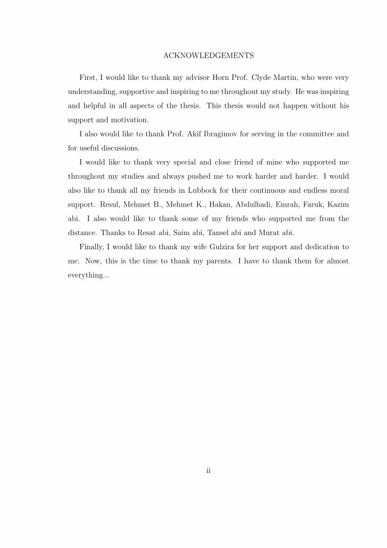
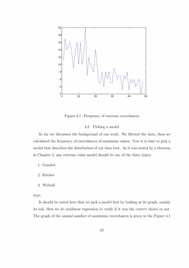
Figure 4.1: Frequency of extreme exceedances
4.2 Picking a model
So far we discussed the background of our work. We filtered the data, then we
calculated the frequency of exceedances of maximum values. Now it is time to pick a
model that describes the distribution of our data best. As it was stated by a theorem
in Chapter 3, any extreme value model should be one of the three types:
1. Gumbel
2. Frechet
3. Weibull
type.
It should be noted here that we pick a model first by looking at its graph, mainly
its tail, then we do nonlinear regression to verify if it was the correct choice or not.
The graph of the annual number of maximum exceedances is given in the Figure 4.1
24
By looking at the graph closely, we see that it can be modeled by Frechet distribution
family.
4.2.1 Picking Frechet distribution type
Suppose F whose tail is of power law form,
1− F (x) ∼ c ∗ x−α
as x →∞ with both c and α ≥ 0
This form covers the Pareto distribution as well as t and F distributions. [7]
Let’s define scaling constants an = (n ∗ c)1/α and bn = 0 and renormalize F.
Then for x > 0
F n(an ∗ x) ≈ (1− c ∗ (an ∗ x)−α)n (4.1)
F n(an ∗ x) = (1− x−α
n)n (4.2)
equation on the above converges to exp(−x−α) for α ≥ 0 [?]
Thus, the limiting distribution is Frechet type.
4.3 Least squares regression of the Model
In the Figure 1.1, the x coordinate represents time(years) between 1914 and 1963.
So, x = 1 refers to the 1914 and so on. Let xi be represented by ti where i = 1...49.
The y coordinate has the values of the number of maximum temperature exceedances
and let yi be represented by βi.
In order to check how well our data fit into the picked Frechet model, we want to
do the least squares regression. Putting the values into the equation, we get:
f(α) =1
2∗
49∑i=1
(exp(−ti)−αi − βi)
2 (4.3)
Since this is a nonlinear equation, we will solve this iteratively by using the Matlab.
In fact, we use Newton’s method to solve f(α). Recall that Newton’s method is :
ki+1 = ki − f(x)
f ′(x)(4.4)
25
As we see above equation, we need first and second derivative of f(α).
Differentiating the equation 4.5 with respect to α using maple we get
f ′(α) =49∑i=1
(exp(−ti)−αi − βi) ∗ x−α ∗ ln(ti) ∗ exp(−ti)
−αi (4.5)
Taking the second derivative of f(α) with respect to α yields:
f ′′(α) =49∑i=1
[(−ti−αi)2 ∗ ln(ti)
2 ∗ (exp(−ti)−αi)2]−
−49∑i=1
[(exp(−ti)−αi − βi) ∗ x−α ∗ ln(ti)
2 ∗ exp(−ti)−αi ]+
+49∑i=1
[(exp(−ti)−αi − βi) ∗ x−α ∗ ln(ti)
2 ∗ exp(−ti)−αi ]
Here we attach the matlab code for this nonlinear least squares fit that we dis-
cussed above:
% This code is for the least squares fit of the data.
% The original equation is given in a seperate sheet.
% Here we look only on the numerical part of the solution
% This program solves the nonlinear equation by using the
% Newton’s method.
clear
clc
xz = 1;
for i = 1:49
t(i,1) = xz;
i = 1+i;
xz = xz+1;
end
for i = 1:49
26
a(i,1) = exp(t(i,1));
i = i+1;
end
% vector alfa stores the number of exceedances of the maximum
%temperature in each year between 1914 and 1963
alfa = [11 17 14 15 16 13 9 13 16 10 16 10 13 20 7 12 10 9 8
14 10 5 5 8 4 8 6 8 5 5 9 8 6 7 7 3 7 6 8 3 6 5 6 4
5 6 2 5 5]’;
% now k will be calculated iteratively.
% v1 is used to store the values of the first derivative
% w is used to store the values of the second derivative for
%the sake of % clarity, I split it into two parts.
v1 = 0;
v2 = 0;
w1 = 0;
w2 = 0;
v = 0;
w = 0;
k(1,1) = 0;
j = 1;
for l = 1:10
for i = 1:49
v = v + ((exp(-t(i,1)^(-k(j,1))))-alfa(i,1))
*t(i,1)*(t(i,1))^(-k(j,1))*log(t(i,1))*
*exp((-t(i,1))^(-k(j,1)));
w1 = (t(i,1)^(-k(j,1)))^2*(log(t(i,1)))^2*
*(exp(-t(i,1)^(-k(j,1))))^2;
w2 = ((exp(-t(i,1)^(-k(j,1))))-alfa(i,1))*
27
*(t(i,1))^(-k(j,1))*
(log(t(i,1)))^2*(exp(-t(i,1)^(-k(j,1))));
w3 = (exp(-t(i,1)^(-k(j,1)))-alfa(i,1))*
*(t(i,1)^(-k(j,1)))^2*
(log(t(i,1)))^2*exp(-t(i,1)^(-k(j,1)));
w = w1-w2+w3;
i = i+1;
end
j = j+1;
k(j,1) = k(j-1,1)-(v/w);
l = l+1;
i = 1;
end
Solution of the above equation yields α = 3.3717 ∗ 104
4.4 Conclusion
In this thesis, we worked with data which is the maximum daily temperatures
between 1913 and 1963. Our goal was to use the statistical methodology called
Extreme Value Theory to support the idea that there is a global warming. We
have applied Gumbel and Frechet distributions from Block Maximum Model to our
data and the result that we obtained contradicts with the fact of existence of Global
warming. Therefore, we conclude that Extreme Value Theory does not work for this
type problem. We think the reasons of Extreme Value Theory methods not working
for this problem might be:
1. The underlying probability distribution is changing
2. There might be some very important factors that we did not consider for this
problem
28
BIBLIOGRAPHY [1] Global warming, Retrieved September 8, 2006, from http://www.globalwarming.org, (n.d.). [2] American Geophysical Union (AGU), Human impacts on climate. Retrieved September 10, 2006, from http://www.agu.org/sci_soc/policy/climate_change_position.html, (n.d.). [3] World wild life, Retrived October 2, 2006, from www.worldwildlife.org, (n.d.). [4] Smith, R. Lecture notes on environmental statistics. Lecture presented at University of North Carolina, Chapel Hill, NC. Retrieved September 15, 2006, from http://www.stat.unc.edu/postscript/rs/envnotes.pdf. (n.d.). [5] Katz, R. Statistics of weather and climate extremes. Retrieved September 3, 2006, from www.isse.ucar.edu/extremevalues/extreme.html, (n.d.). [6] Embrechts, P. Resnick, S. & Samorodnitsky, G. Extreme value theory as a risk management tool. North American Actuarial Journal, 3, 30-41, (1999). [7] Coles, S. An introduction to statistical modeling of extreme values. New York: Springer, (2001).
29
PERMISSION TO COPY
In presenting this thesis in partial fulfillment of the requirements for a master’s
degree at Texas Tech University or Texas Tech University Health Sciences Center, I
agree that the Library and my major department shall make it freely available for
research purposes. Permission to copy this thesis for scholarly purposes may be granted
by the Director of the Library or my major professor. It is understood that any copying
or publication of this thesis for financial gain shall not be allowed without my further
written permission and that any user may be liable for copyright infringement.
Agree (Permission is granted.)
___________Bahtiyar Babanazarov __________________ ______11/20/06__ Student Signature Date Disagree (Permission is not granted.) _______________________________________________ _________________ Student Signature Date