1

DISTRIBUTION PLANNING

CONSIDERING WAREHOUSING DECISIONS

Pratik J. Parikh, Xinhui Zhang, and Bhanuteja Sainathuni

Wright State University

Abstract

Modern supply chains heavily depend on warehouses for rapidly

fulfilling customer demands through retail, web-based, and catalogue

channels. The traditional approach that considers warehouses as cost-

centers has affected the profitability of numerous supply chains. A lack of

synchronization between procurement and allocation decisions causes

warehouses to scramble for resources during peak times and be faced with

under-utilized resources during drought times. Warehouses, however, have

emerged as service-centers and it is imperative that warehousing decisions

be an integral part of supply chain decisions. In this paper we propose a

mixed-integer programming model to integrate warehousing decisions

with those of inventory and transportation to minimize long-run

distribution cost. Preliminary experiments suggest a sizeable reduction in

the level and variance in the warehouse workforce requirements. A cost

savings ranging between 2-6% is also realized.

1 Motivation According to the 20th State of the Logistics Report [5], logistics costs comprise of 9.4%

of the U.S. GDP, which accounts to about $1,309B dollars. Warehousing costs rose

almost 10% from 2007 to 2008 to $122B dollars across 600,000 small and large

warehouses in the nation. Warehouses, however, are often considered as cost centers and

treated outside the realms of supply chain planning and optimization. Consequently,

warehouse managers are often squeezed between their procurement department and the

allocation department (or stores). The procurement department determines the quantity of

products to be purchased from vendors and subsequently stocked at the warehouse to

reap maximum benefits from quantity discounts. The centralized allocation department

(or decentralized store ordering) determines the quantity to be delivered from warehouses

to stores in order to minimize the inventory and/or transportation costs. Both these

decisions often cause a large variation in the inbound and outbound shipments at the

warehouse resulting in an imbalance in warehouse’s workload. Warehouse managers

often scramble for resources during peak-times resulting in hiring temporary workers

and/or paying overtime, and have trouble generating enough work during slow times

resulting in underutilized resources.

2

The problem we consider was motivated by our general observation in industry and

specifically at the warehouse of our industry partner --- an U.S-based apparel supply

chain. The warehouse at this apparel supply chain operates in a reactive mode; that is,

warehousing decisions are made after the procurement and allocation decisions.

Consequently, depending on the timing and quantity of products received by and shipped

from the warehouse, the workforce utilization varies significantly. We observed that

during a 5-day week the workforce utilization varied from 50% to 150%, a staggering

300% variation. This has cost the company millions of dollars annually due to operating

inefficiencies at the warehouse. This begs the question, how would a supply chain benefit

if it proactively accounted for warehousing decisions at the planning stage, instead of

warehouses having to react?

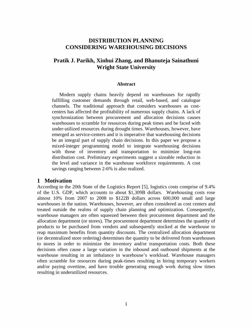
To address this question, we introduce the integrated warehousing-inventory-

transportation problem (WITP) that jointly considers warehouse utilization and

capacities, along with inventory and transportation decisions to identify an optimal

distribution strategy (see Figure 1). The focus of WITP is to determine the optimal

allocation and distribution of products from vendors to stores via warehouses such that

total distribution cost is minimized.

(a) (b)

V2

W1

W2

V1

S1 S3 S4S2

INB

OU

ND

OU

T B

OU

ND

WAREHOUSE

UTILIZATION

M T W R FINVENTORY

M T W R F

TRANSPORTATION W I T P

WAREHOUSING

INVENTORY TRANSPORTATION

I R P

Figure 1: The Warehousing, Inventory, and Transportation Decisions and their Integration in a

Multi-Echelon Supply Chain.

The remaining part of this paper is outlined as follows. In Section 2 we briefly review

academic literature in this area. In Section 3 we provide details of the WITP and present a

cost model for estimating workforce cost at a warehouse. Section 4 presents a

mathematical programming model for the WITP. Results based on preliminary

experiments are presented in Section 5, followed by a summary in Section 6.

2 Literature Review Recent years have seen a significant thrust on integrating transportation decisions with

inventory in supply chain. The objective has been to trade-off inventory-related and

3

transportation-related costs to minimize supply chain cost. We briefly review integrated

models proposed for centralized supply chains.

The presence of a centralized system has led to the questions of when to deliver

(timing), how much to deliver (quantity), and how to deliver (mode and routing). From a

research standpoint, a popular integrated problem in this area is the inventory-routing

problem (IRP), which refers to developing a repeatable distribution strategy that

minimizes transportation costs and the number of stock-outs. Both deterministic and

stochastic IRP-versions have been introduced in the literature [3, 9]. Abdelmaguid and

Dessouky [1] argued that the primary focus of the IRP is on minimizing the total

transportation cost, with little consideration for inventory costs. Consequently, they

propose an integrated inventory-distribution problem (IDP) that considers inventory and

transportation costs, allowing backorders, in a multi-period setting. In essence, they

suggest that the IRP is a relaxation of the IDP. They present a nonlinear mixed integer

programming model for the IDP and solve it using genetic algorithm. They specifically

designed the mutation part in the improvement phase of genetic algorithm to investigate

partial deliveries, as they can provide significant reductions in transportation and shortage

costs.

Lei et al. [10] considered the production-inventory-distribution-routing problem

(PIDRP), where the focus is on coordinating the production and transportation schedules

between a set of vendors and a set of customers (which could be warehouses). They solve

a multi-plant, multi-DC, and multi-period PIDRP using a two-stage sequential approach.

Bard and Nananukul [2] solved a one-plant, multi-customer PIDRP assuming a single

mode of transportation by employing a reactive tabu search algorithm with path-

relinking. Their study differs from the traditional IRP as it considers the trade-off

between production decision and inventory level at the facility.

Cetinkaya et al. [4] presented a renewal theoretic model to compute parameters of an

integrated inventory-transportation policy where demand follows a general stochastic

process. Their research considered one-echelon, one-vendor, one-customer, and one-

product scenario, unit transportation cost that includes handling (loading the truck), and

inventory related costs at vendor’s warehouse. However, they did not capture

warehousing costs related to key activities, such as unloading, put-away, picking, and

cross-docking in their model.

In the area of warehousing academic literature has focused primarily on warehouse

location, design, and operation. White and Francis [15] were probably the first

researchers to develop quantitative models to decide between private and leased

warehouses. Since then numerous models have been developed to assist in warehouse

design, more specifically sizing [6, 8, 11] aisle-layout [7, 14], and operational aspects

[12, 13].

From our review of the literature, and industry-practice, we know of no research or

tool that integrates warehousing, inventory, and transportation decisions in a single

optimization framework. We believe that such integration has the potential of reducing

supply chain costs significantly. We now provide details of our proposed research, along

with our preliminary work in this area.

4

3 The Warehouse-Inventory-Transportation Problem The warehousing-inventory-transportation problem (WITP) is to determine the optimal

allocation and distribution of product from vendor to stores via one or more warehouses

with the objective of minimizing long-term distribution cost. This problem jointly

considers warehousing, inventory, and transportation, and addresses the following

questions:

When and in what quantity of each product to order from vendors to replenish

warehouses?

When and what quantities to deliver from warehouses to stores, and which

warehouse to source from?

Is drop-shipping certain products from vendors to stores beneficial?

Which transportation modes and delivery routes to follow?

What level of warehouse workforce (permanent and temporary) should be used?

In the WITP we consider the decision of whether or not to advance or delay

shipments depending upon warehouse’s workforce utilization, space utilization, and

inventory availability. Doing so has cost trade-offs. On one hand, by advancing or

delaying shipments warehouse costs may be reduced by better managing the workload on

a daily basis, thus reducing variation in workforce utilization. Transportation costs may

be reduced due to better consolidation, which may reduce the number of shipments

during the time-horizon. However, the stores and warehouses may run a risk of holding

too much inventory by advancing or delaying shipments.

The WITP integrates relevant warehousing, inventory, and transportation decisions to

tradeoff the associated costs. The warehousing decisions that WITP considers include

space, layout, material handling system, workforce planning and scheduling, utilities, and

alike. For this study, our focus is on workforce planning.

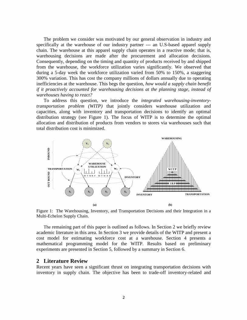
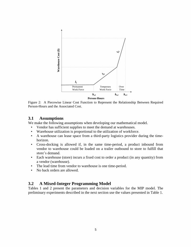
To model warehouse workforce we use the fact that the workforce level is

proportional to the person-hours required for various activities in the warehouse. We

consider five key activities; unloading inbound trailers, put-away, picking, loading

outbound trailers, and cross-docking. We express the relationship between the required

person-hours and the corresponding workforce cost through a piecewise linear cost

function; see Figure 2. The parametric curve in the Figure 2 reflects the way most

warehouses operate; i.e., most have a mix of permanent and temporary employees, with a

possibility of overtime. In the cost function, bw1 and bw2 represent the levels of permanent

and temporary employees, respectively. The region between bw2 and bw3 represents

overtime. We next present our assumptions in developing a mathematical model for the

WITP.

5

Ware

hou

se C

ost

($)

Person-Hours

l1

l 2

l 3

bw1 bw3

Over

Time

Temporary

Work Force

Permanent

Work Force

bw2

Figure 2: A Piecewise Linear Cost Function to Represent the Relationship Between Required

Person-Hours and the Associated Cost.

3.1 Assumptions

We make the following assumptions when developing our mathematical model.

• Vendor has sufficient supplies to meet the demand at warehouses.

• Warehouse utilization is proportional to the utilization of workforce.

• A warehouse can lease space from a third-party logistics provider during the time-

horizon.

• Cross-docking is allowed if, in the same time-period, a product inbound from

vendor to warehouse could be loaded on a trailer outbound to store to fulfill that

store’s demand.

• Each warehouse (store) incurs a fixed cost to order a product (in any quantity) from

a vendor (warehouse).

• The lead time from vendor to warehouse is one time-period.

• No back orders are allowed.

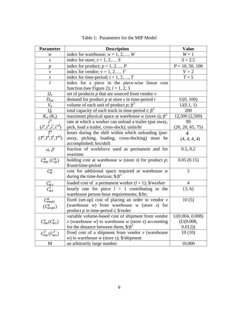
3.2 A Mixed-Integer Programming Model Tables 1 and 2 present the parameters and decision variables for the MIP model. The

preliminary experiments described in the next section use the values presented in Table 1.

6

Table 1: Parameters for the MIP Model

Parameter Description Value

w index for warehouse; w = 1, 2,…, W W = 1

s index for store; s = 1, 2,…, S S = 2,5

p index for product; p = 1, 2,…, P P = 10, 50, 100

v index for vendor; v = 1, 2,…, V V = 2

t index for time-period; t = 1, 2,…, T T = 5

l index for a piece in the piece-wise linear cost

function (see Figure 2); l = 1, 2, 3

Ωv set of products p that are sourced from vendor v

Dspt demand for product p at store s in time-period t U(0, 100)

Vp volume of each unit of product p; ft3 U(0.1, 1)

Qt total capacity of each truck in time-period t; ft3 200

Kw (Ks) maximum physical space at warehouse w (store s); ft3 12,500 (2,500)

λu

(λp,λ

k,λ

l,λ

xd)

rate at which a worker can unload a trailer (put away,

pick, load a trailer, cross-dock); units/hr

90

(20, 20, 65, 75)

Tu

(T

p,T

k,T

l,T

xd)

hours during the shift within which unloading (put-

away, picking, loading, cross-docking) must be

accomplished; hrs/shift

4

(4, 4, 4, 4)

, fraction of workforce used as permanent and for

overtime

0.5, 0.2

( ) holding cost at warehouse w (store s) for product p;

$/unit/time-period

0.05 (0.15)

cost for additional space required at warehouse w

during the time-horizon; $/ft3

5

loaded cost of a permanent worker (l = 1); $/worker 4

hourly rate for piece l > 1 contributing to the

warehouse person-hour requirements; $/hr;

{3, 6}

fixed (set-up) cost of placing an order to vendor v

(warehouse w) from warehouse w (store s) for

product p in time-period t; $/order

10 (5)

(

variable volume-based cost of shipment from vendor

v (warehouse w) to warehouse w (store s) accounting

for the distance between them; $/ft3

U(0.004, 0.008)

(U(0.008,

0.012))

fixed cost of a shipment from vendor v (warehouse

w) to warehouse w (store s); $/shipment

10 (10)

M an arbitrarily large number 10,000

7

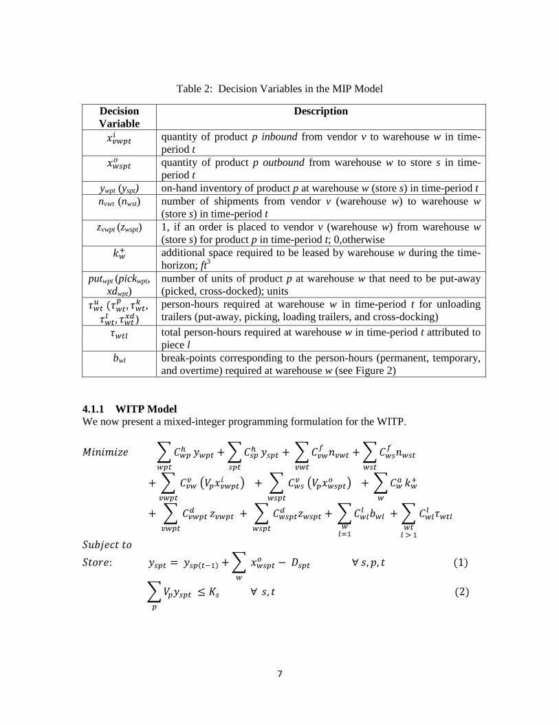
Table 2: Decision Variables in the MIP Model

Decision

Variable

Description

quantity of product p inbound from vendor v to warehouse w in time-

period t

quantity of product p outbound from warehouse w to store s in time-

period t

ywpt (yspt) on-hand inventory of product p at warehouse w (store s) in time-period t

nvwt (nwst) number of shipments from vendor v (warehouse w) to warehouse w

(store s) in time-period t

zvwpt (zwspt) 1, if an order is placed to vendor v (warehouse w) from warehouse w

(store s) for product p in time-period t; 0,otherwise

additional space required to be leased by warehouse w during the time-

horizon; ft3

putwpt (pickwpt,

xdwpt)

number of units of product p at warehouse w that need to be put-away

(picked, cross-docked); units

)

person-hours required at warehouse w in time-period t for unloading

trailers (put-away, picking, loading trailers, and cross-docking)

total person-hours required at warehouse w in time-period t attributed to

piece l

bwl break-points corresponding to the person-hours (permanent, temporary,

and overtime) required at warehouse w (see Figure 2)

4.1.1 WITP Model

We now present a mixed-integer programming formulation for the WITP.

8

The objective of the above model is to minimize the total distribution cost. The cost

elements considered include transportation (fixed and variable), holding at warehouse

9

and store, additional warehouse space, and workforce required at the warehouse.

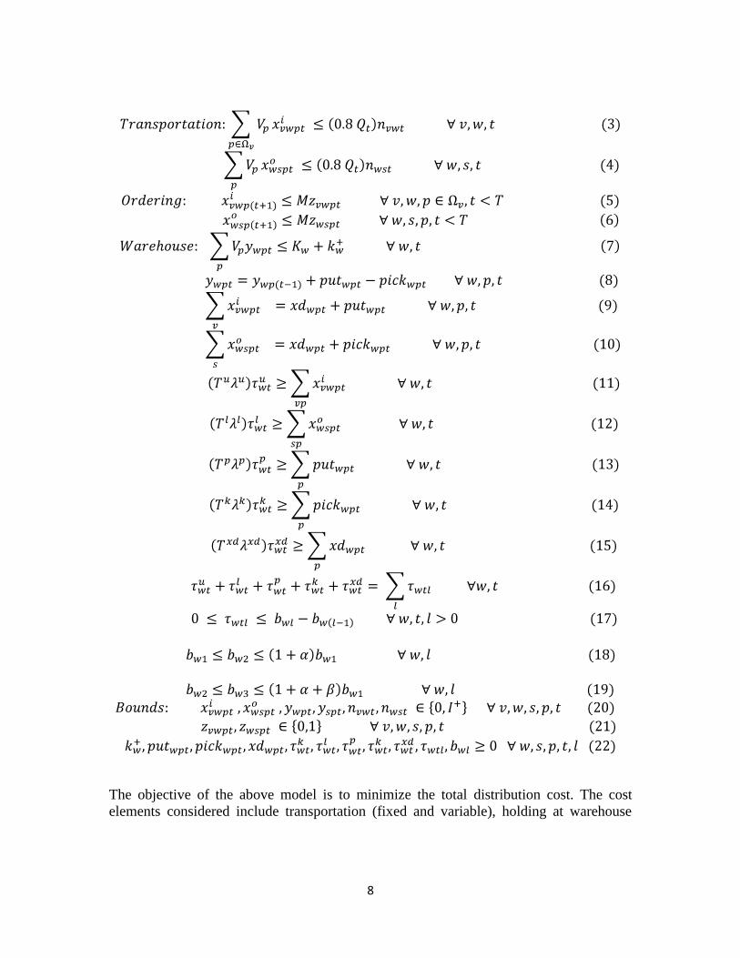
Constraints (1) and (2) are related to stores, Constraints (3) and (4) to transportation,

Constraints (5) and (6) to order setup, and Constraints (7)-(19) to warehouse space and

workforce.

Constraint (1) calculates the on-hand inventory for each product at a store in the

current time-period depending on the on-hand inventory in the previous time-period,

quantity delivered from warehouses, and the demand at the store. Constraint (2) imposes

space constraint at each store.

The transportation capacities (volume-based) for vendor-to-warehouse and

warehouse-to-store are modeled through Constraints (3) and (4). Because we do not

consider the geometry of the trailer and the products, we restrict the trailer-fill rate to

80% of its volumetric capacity to ensure practical feasibility of loading products in the

trailer. Constraints (5) and (6) are used to find if an order is placed by a warehouse (store)

to a vendor (warehouse) for a product in a time-period.

Constraint (7) calculates the actual space required at a warehouse allowing for the

provision of leasing additional space during the time-horizon. Constraint (8) calculates

the on-hand inventory at a warehouse. Constraint (9) balances inbound quantities at the

warehouse with cross-docked and put-away quantities, while Constraint (10) balances

outbound quantities with cross-docked and picked quantities. The required hours for

unloading, put-away, picking, loading, and cross-docking are calculated by Constraints

(11)-(15). Constraint (16) calculates the required person-hours at the warehouse to

accomplish the five activities during the time-period. Constraint (17) satisfies the

incremental person-hours requirement; i.e., first use the permanent workforce, then use

temporary, and finally overtime. The requirement that temporary workforce cannot be

more than a certain fraction, , of the permanent workforce at each warehouse is

modeled by Constraint (18). Essentially, we are trying to identify the level of permanent

and temporary workforce, corresponding to break-points bw1 and bw2, respectively, for the

time-horizon. Constraint (19) indicates that the allowed overtime at a warehouse is

restricted to a certain fraction, β, of the permanent workforce. Constraints (20)-(22)

specify bounds on the decision variables.

5 Preliminary Experiments

To evaluate the benefits of the WITP approach, we compare the total distribution cost

obtained from the model for WITP to that obtained by sequentially solving the models for

ITP (inventory-transportation problem) and WP (warehouse problem). We believe this

sequential approach is the current norm in academic literature and industry.

The models for ITP and WP are obtained by decomposing the model for WITP. That

is, the model for ITP includes the inventory, transportation, and ordering constraints and

associated cost terms in the objective function, while the model for WP includes only the

warehousing constraints. Both these models are presented below.

10

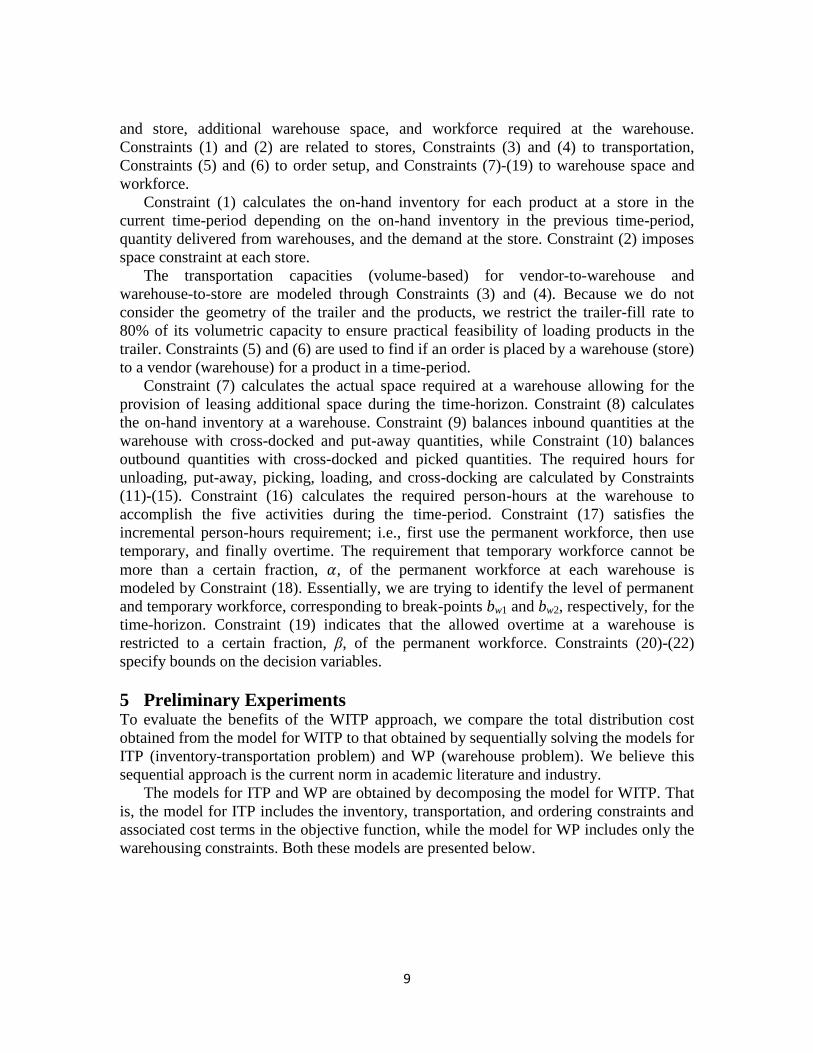
Model for the Inventory-Transportation Problem (ITP)

Subject to: Constraint-sets (1) – (7) from WITP model

Model for the Warehousing Problem (WP)

Subject to: Constraint-sets (9) – (19) from WITP model

For a given data-set, the optimal solution of ITP provides information about inbound

and outbound quantities, warehouse and store inventories, shipments, and ordering. These

inbound and outbound quantities, along with warehouse inventory, are used as inputs in

the WP model. The optimal solution to the WP provides information about the workforce

level at the warehouse, which helps in calculating the warehousing cost. The total

distribution cost is then calculated as the sum of inventory, transportation, warehousing,

and order set-up costs obtained from both the models.

The total distribution cost resulting from the sequential approach (ITP+WP) is then

compared with the optimized solution of integrated WITP model. We also compare the

required person-hours for each time-period in the warehouse, and the optimal break-

points for all the three types of work forces (permanent, temporary, and over-time) in

both the approaches, WITP and ITP+WP. These comparisons are presented in the next

section.

11

5.1 Experimental Set-Up

The optimization models for ITP, WP, and WITP were solved using xPress Optimization

software version 12.0. All the computations were performed on a system with 2.53 GHz

processor and 512 MB RAM. Several experiments were run with various data-sets to

gauge the performance of the solver on these problems. Through initial experiments we

observed that though the LP solution was obtained in a few seconds the solver could not

obtain optimal solution or prove optimality of the current best solution within 12 hours.

Based on these initial experiments, we decided to conduct our preliminary experiments

with the following four data-sets:

DS1: v2w1s2p10t5

DS2: v2w1s2p50t5

DS3: v2w1s5p50t5

DS4: v2w1s5p100t5

where v2w1s2p10t5 stands for 2 vendors, 1 warehouse, 2 stores, 10 products, and 5 time-

periods.

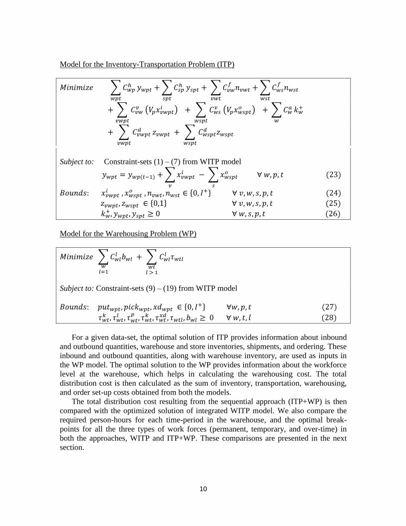
6 Results and Discussion The costs of different components (inventory, transportation, warehousing, and order set-

up) and the %-savings obtained from the model for WITP, as compared to the sequential

ITP+WP approach, are shown in Table 3. A key thing to observe from these results, apart

from the 2-6% savings in the total distribution cost, is that the WITP is able to reduce the

person-hours at the warehouse in each time-period compared to the ITP+WP approach.

Table 3: Comparison of results obtained from the models for ITP+WP and WITP for

four data-sets. (Note: DS = Data-Set, IC = Inventory Cost, TC = Transportation Cost,

WC = Warehousing Cost, SC = Order Set-Up Cost, ∑C = Total Cost, WHBP =

Warehouse Break-Points)

Savings

DS IC TC WC SC ∑C WHBP (hrs) IC TC WC SC ∑C WHBP (hrs) %

$ $ $ $ $ b1,b2,b3 $ $ $ $ $ b1,b2,b3

DS1 220 555 359 410 1544 14,21,24 182 555 204 520 1460 8,12,13 5.45

DS2 1042 2929 1805 2075 7852 73,110,125 838 2929 1096 2500 7364 41,61,70 6.21

DS3 1410 7602 2979 5035 17025 118,177,201 1037 7602 2512 5520 16672 96,145,164 2.08

DS4 2583 12680 5982 10310 31555 229,343,389 1844 12680 5063 11260 30846 185,277,314 2.24

WITPITP + WP

For example, for the data-set DS2 (v1w1s2p50t5), we observe a 6.2% of savings in

the total cost, accounting mostly due to the differences in the warehousing costs. The

model for WITP was able to reduce the warehousing costs from $1,805.27 to $1,095.93,

a reduction of nearly 40%. However, the increase in the order set-up cost did reduce these

savings quite a bit.

12

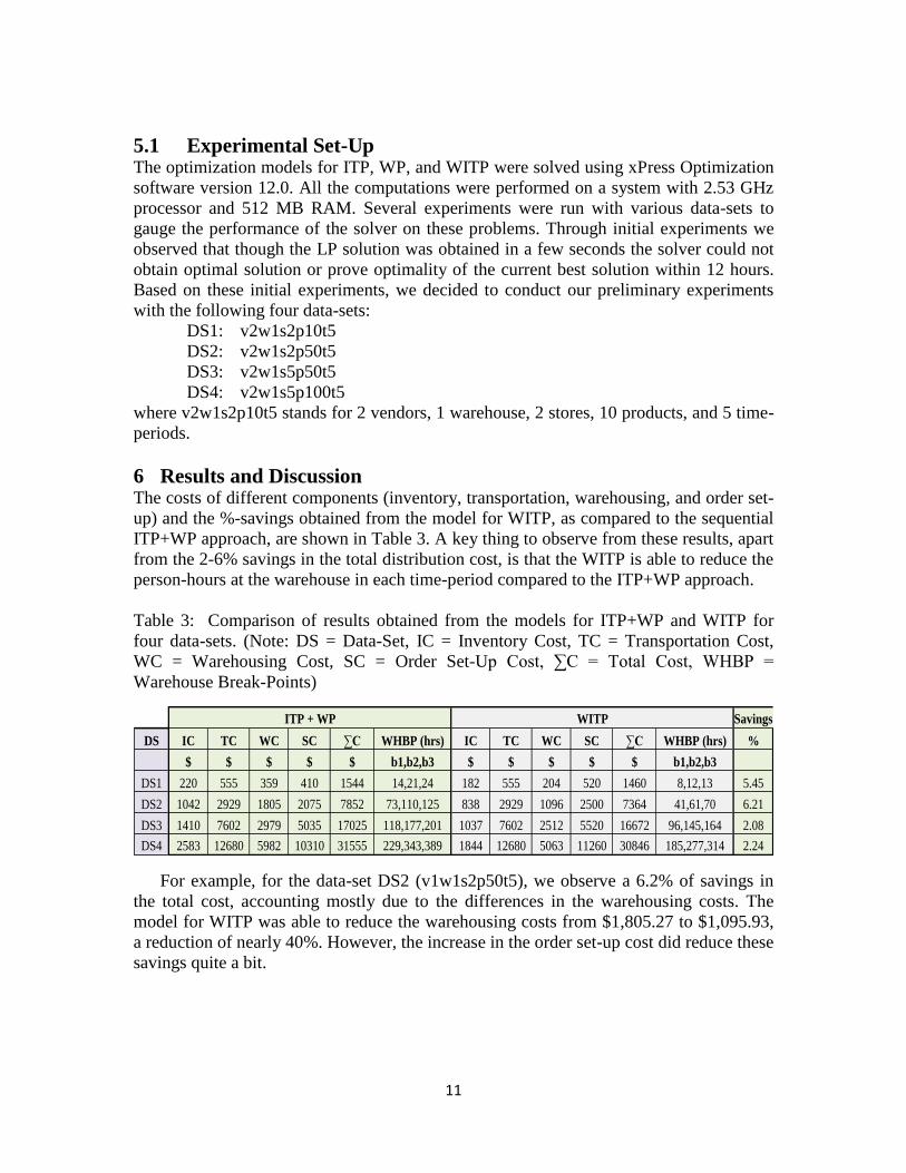
Figures 3-6 represent the differences between the WITP and ITP+WP approaches

with respect to the required number of person-hours in each time-period. From Figure 3

we observe that, for the ITP+WP approach, in time-periods 1 and 4, the number of

required person-hours is relatively high requiring overtime to accomplish the workload

during that time-period. However, during time-periods 2 and 5 the workload was

relatively low resulting in no need for overtime hours; in fact, no temporary workers are

required during time-period 5. Such a large variation in the amount of workload across

time-periods in a time-horizon is commonly experienced by many warehouses, and

makes it relatively difficult for the warehouse manager to plan the workforce.

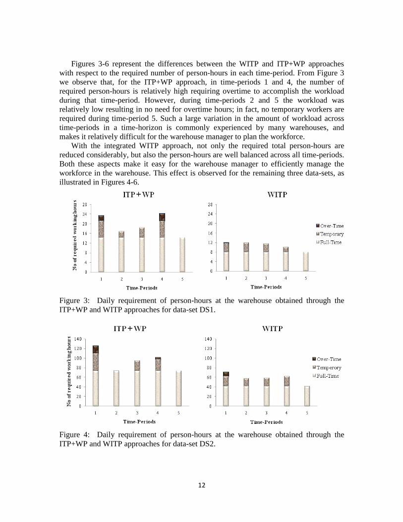
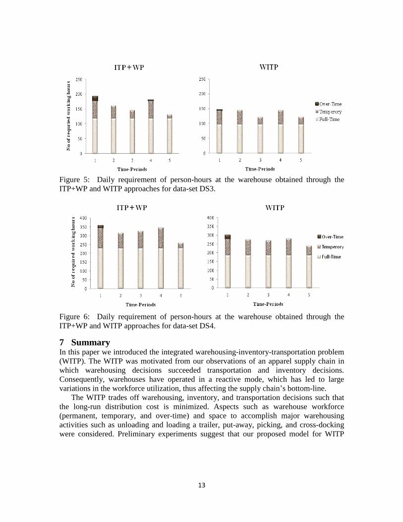
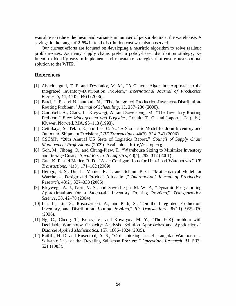
With the integrated WITP approach, not only the required total person-hours are

reduced considerably, but also the person-hours are well balanced across all time-periods.

Both these aspects make it easy for the warehouse manager to efficiently manage the

workforce in the warehouse. This effect is observed for the remaining three data-sets, as

illustrated in Figures 4-6.

Figure 3: Daily requirement of person-hours at the warehouse obtained through the

ITP+WP and WITP approaches for data-set DS1.

Figure 4: Daily requirement of person-hours at the warehouse obtained through the

ITP+WP and WITP approaches for data-set DS2.

13

Figure 5: Daily requirement of person-hours at the warehouse obtained through the

ITP+WP and WITP approaches for data-set DS3.

Figure 6: Daily requirement of person-hours at the warehouse obtained through the

ITP+WP and WITP approaches for data-set DS4.

7 Summary In this paper we introduced the integrated warehousing-inventory-transportation problem

(WITP). The WITP was motivated from our observations of an apparel supply chain in

which warehousing decisions succeeded transportation and inventory decisions.

Consequently, warehouses have operated in a reactive mode, which has led to large

variations in the workforce utilization, thus affecting the supply chain’s bottom-line.

The WITP trades off warehousing, inventory, and transportation decisions such that

the long-run distribution cost is minimized. Aspects such as warehouse workforce

(permanent, temporary, and over-time) and space to accomplish major warehousing

activities such as unloading and loading a trailer, put-away, picking, and cross-docking

were considered. Preliminary experiments suggest that our proposed model for WITP

14

was able to reduce the mean and variance in number of person-hours at the warehouse. A

savings in the range of 2-6% in total distribution cost was also observed.

Our current efforts are focused on developing a heuristic algorithm to solve realistic

problem-sizes. As many supply chains prefer a policy-based distribution strategy, we

intend to identify easy-to-implement and repeatable strategies that ensure near-optimal

solution to the WITP.

References

[1] Abdelmaguid, T. F. and Dessouky, M. M., “A Genetic Algorithm Approach to the

Integrated Inventory-Distribution Problem,” International Journal of Production

Research, 44, 4445–4464 (2006).

[2] Bard, J. F. and Nananukul, N., “The Integrated Production-Inventory-Distribution-

Routing Problem,” Journal of Scheduling, 12, 257–280 (2008).

[3] Campbell, A., Clark, L., Kleywegt, A., and Savelsberg, M., “The Inventory Routing

Problem,” Fleet Management and Logistics, Crainic, T. G. and Laporte, G. (eds.),

Kluwer, Norwell, MA, 95–113 (1998).

[4] Cetinkaya, S., Tekin, E., and Lee, C. Y., “A Stochastic Model for Joint Inventory and

Outbound Shipment Decisions,” IIE Transactions, 40(3), 324–340 (2006).

[5] CSCMP, “20th Annual US State of Logistics Report,” Council of Supply Chain

Management Professional (2009). Available at http://cscmp.org.

[6] Goh, M., Jihong, O., and Chung-Piaw, T., “Warehouse Sizing to Minimize Inventory

and Storage Costs,” Naval Research Logistics, 48(4), 299–312 (2001).

[7] Gue, K. R. and Meller, R. D., “Aisle Configurations for Unit-Load Warehouses,” IIE

Transactions, 41(3), 171–182 (2009).

[8] Heragu, S. S., Du, L., Mantel, R. J., and Schuur, P. C., “Mathematical Model for

Warehouse Design and Product Allocation,” International Journal of Production

Research, 43(2), 327–338 (2005).

[9] Kleywegt, A. J., Nori, V. S., and Savelsbergh, M. W. P., “Dynamic Programming

Approximations for a Stochastic Inventory Routing Problem,” Transportation

Science, 38, 42–70 (2004).

[10] Lei, L., Liu, S., Ruszczynski, A., and Park, S., “On the Integrated Production,

Inventory, and Distribution Routing Problem,” IIE Transactions, 38(11), 955–970

(2006).

[11] Ng, C., Cheng, T., Kotov, V., and Kovalyov, M. Y., “The EOQ problem with

Decidable Warehouse Capacity: Analysis, Solution Approaches and Applications,”

Discrete Applied Mathematics, 157, 1806–1824 (2009).

[12] Ratliff, H. D. and Rosenthal, A. S., “Order-picking in a Rectangular Warehouse: a

Solvable Case of the Traveling Salesman Problem,” Operations Research, 31, 507–

521 (1983).

15

[13] Parikh, P. J. and Meller, R. D., “A Travel-Time Model for an Order Picking System

Employing a Person-Onboard Equipment,” European Journal of Operational

Research, 200(2), 385–394 (2010).

[14] Roodbergen, K. J. and Vis, I. F. A., “A Model for Warehouse Layout,” IIE

Transactions, 38(10), 799–812 (2006).

[15] White, J. A. and Francis, R. L., “Normative Models for Some Warehouse Sizing

Problems,” AIIE Transactions, 9(3), 185–190 (1971).