Distribution Ray Tracing

In Whitted Ray Tracing we computed lighting very crudely

Phong + specular global lighting

In Distributed Ray Tracing we want to compute the lighting as accurately as possiblelighting as accurately as possible

Use the formalism of RadiometryCompute irradiance at each pixel (by integrating all the i i li ht)incoming light) Since integrals are can not be done analytically, we will employ numeric approximationsy

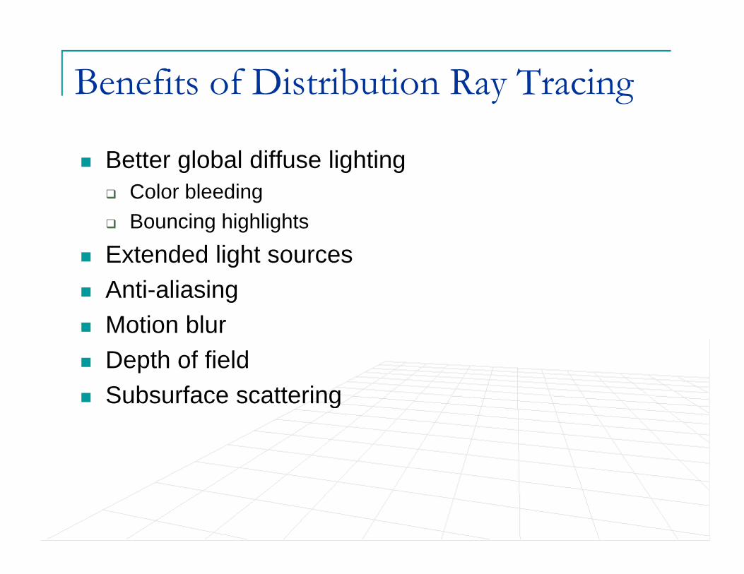
Benefits of Distribution Ray Tracing

Better global diffuse lightingColor bleedingBouncing highlights

Extended light sourcesExtended light sourcesAnti-aliasingMotion blurMotion blurDepth of fieldSubsurface scatteringSubsurface scattering

Radiance at a PointRecall that radiance (shading) at a surface point is given by

ωρ ddndpLdddpL iii )(),(),(),(rrrrrr

⋅−= ∫If we parameterize directions in spherical coordinates and assume small differential solid angle we get

ωρ ddndpLdddpL iiiee )(),(),(),( ∫Ω

and assume small differential solid angle, we get( ) ( )( ) φθθθφθφθφρ

πφ πθ

dddndpLdddpL iiiee ∫ ∫∈ ∈

⋅−=]2,0[ ]2,0[

sin),(),(,),(,),(rrrrrr

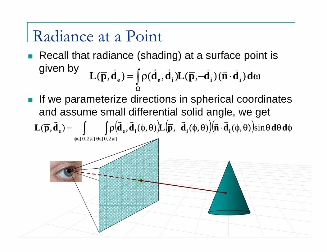
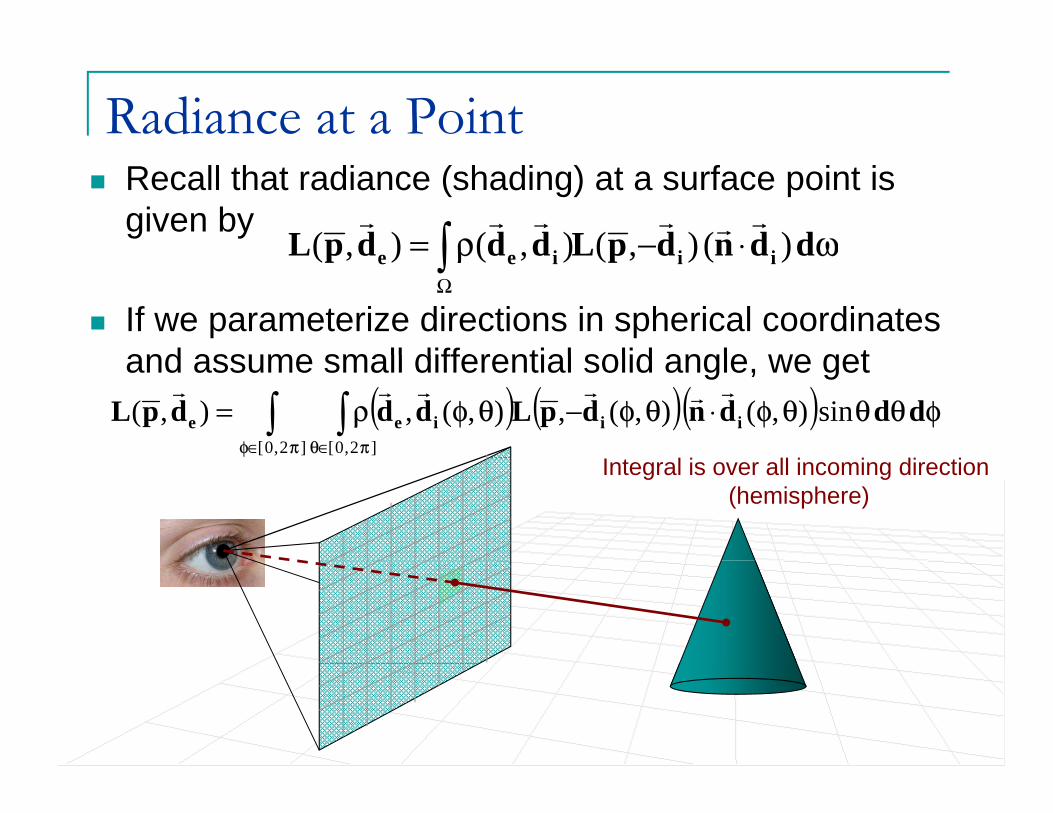
Radiance at a PointRecall that radiance (shading) at a surface point is given by

ωρ ddndpLdddpL iii )(),(),(),(rrrrrr

⋅−= ∫If we parameterize directions in spherical coordinates and assume small differential solid angle we get

ωρ ddndpLdddpL iiiee )(),(),(),( ∫Ω

and assume small differential solid angle, we get( ) ( )( ) φθθθφθφθφρ

πφ πθ

dddndpLdddpL iiiee ∫ ∫∈ ∈

⋅−=]2,0[ ]2,0[

sin),(),(,),(,),(rrrrrr

I l i ll i i di iIntegral is over all incoming direction (hemisphere)

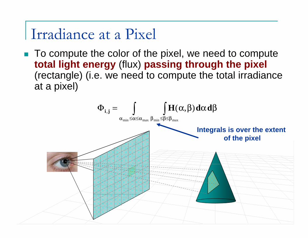
Irradiance at a PixelTo compute the color of the pixel, we need to compute total light energy (flux) passing through the pixel(rectangle) (i e we need to compute the total irradiance(rectangle) (i.e. we need to compute the total irradiance at a pixel)

∫ ∫ βαβαααα βββ

ddHji ),(maxmin maxmin

, ∫ ∫≤≤ ≤≤

=Φ

Integrals is over the extent of the pixel

Numerical Integration (1D Case)Remember: integral is an area under the curveWe can approximate any integral numerically asWe can approximate any integral numerically as follows

xiy

)(xfid

xD

∫DN

∫∑=

∞→⎯⎯ →⎯i

Nii dxxfxfd01

)()(

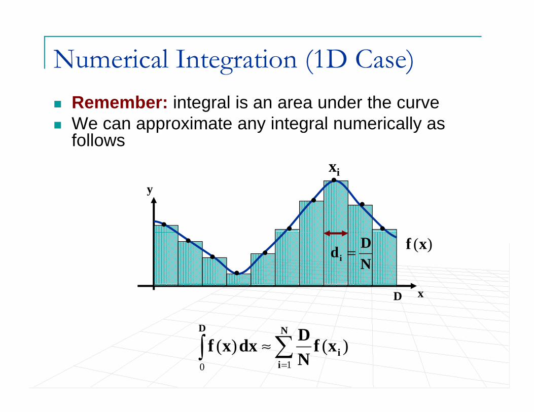
Numerical Integration (1D Case)Remember: integral is an area under the curveWe can approximate any integral numerically asWe can approximate any integral numerically as follows

xiy

)(xfNDdi =

D

∫ND D

x

∑∫=

≈i

ixfNDdxxf

10

)()(

Numerical Integration (1D Case)Problem: what if we are really unlucky and our signal has the same structure as sampling?signal has the same structure as sampling?

xiy

)(xf

D

∫ND D

x

∑∫=

≈i

ixfNDdxxf

10

)()(

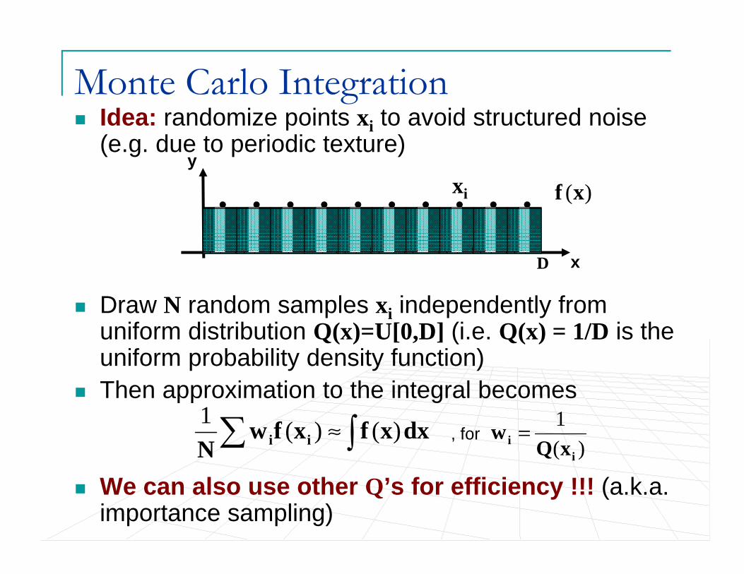
Monte Carlo IntegrationIdea: randomize points xi to avoid structured noise (e.g. due to periodic texture)

y

)(xfxi

Draw N random samples xi independently from if di t ib ti Q( ) U[0 D] (i Q( ) 1/D i th

xD

uniform distribution Q(x)=U[0,D] (i.e. Q(x) = 1/D is the uniform probability density function)Then approximation to the integral becomesThen approximation to the integral becomes

∑ ∫≈ dxxfxfwN ii )()(1

)(1

ii xQ

w =, for

We can also use other Q’s for efficiency !!! (a.k.a. importance sampling)

Monte Carlo Integration

xiy

)(xf

D

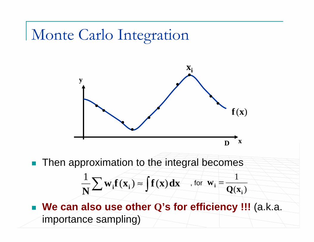
Then approximation to the integral becomes

x

pp g

∑ ∫≈ dxxfxfwN ii )()(1

)(1

ii xQ

w =, for

We can also use other Q’s for efficiency !!! (a.k.a. importance sampling)

Stratified SamplingIdea: combination of uniform sampling plus random jitterBreak domain into T intervals of widths d and NBreak domain into T intervals of widths dt and Ntsamples in interval t

y dt

)(xf

Integral approximated using the following:D x

Integral approximated using the following:

∑ ∑= =

T

tjt

N

jt

t

xfdN

t

1,

1)(1

Stratified SamplingIf intervals are uniform dt = D/T and there are same number of samples in each interval Nt = N/T then this

i ti d t T Napproximation reduces to:

The interval size and the # of samples can vary !!!

∑∑= =

T

tjt

N

jxf

NDt

1,

1)(

The interval size and the # of samples can vary !!!

y dt

)(xf

Integral approximated using the following:

)(

D xIntegral approximated using the following:

∑ ∑= =

T

tjt

N

jt

t

xfdN

t

1,

1)(1

Back to Distribution Ray TracingBased on one of the approximate integration approaches we need to compute

Let’s try uniform sampling

( ) ( )( ) φθθθφθφθφρπφ πθ

dddndpLdddpL iiiee ∫ ∫∈ ∈

⋅−=]20[ ]20[

sin),(),(,),(,),(rrrrrr

πφ πθ∈ ∈]2,0[ ]2,0[

( ) ( )( ) φθθθφθφθφρ ΔΔ⋅−≈∑∑= =

sin),(),(,),(,1 1

M

m

N

nnminminmie dndpLdd

rrrrr

= =1 1m n

πθ 2/Δθθ Δ⎟⎞⎜⎛ 1n

where

N

Mπφ

θ

2=Δ

=Δ

φφ

θθ

Δ⎟⎠⎞

⎜⎝⎛ −=

Δ⎟⎠

⎜⎝

−=

21

2

m

n

m

n

N⎠⎝ 2

midpoint of the interval (sample point) Interval width

Importance Sampling in Distribution Ray Tracing

Problem: Uniform sampling is too expensive (e.g. p g p ( g100 samples/hemisphere with depth of ray recursion of 4 => 1004=108 samples per pixel … with 105 pixels =>1015 samples)>10 samples)

Solution: Sample more densely (using importance p y ( g psampling) where we know that effects will be most significant

Direction toward point or extended light source areDirection toward point or extended light source are significantSpecular and off-axis specular are significantTexture/lightness gradients are significantTexture/lightness gradients are significant Sample less with greater depth of recursion

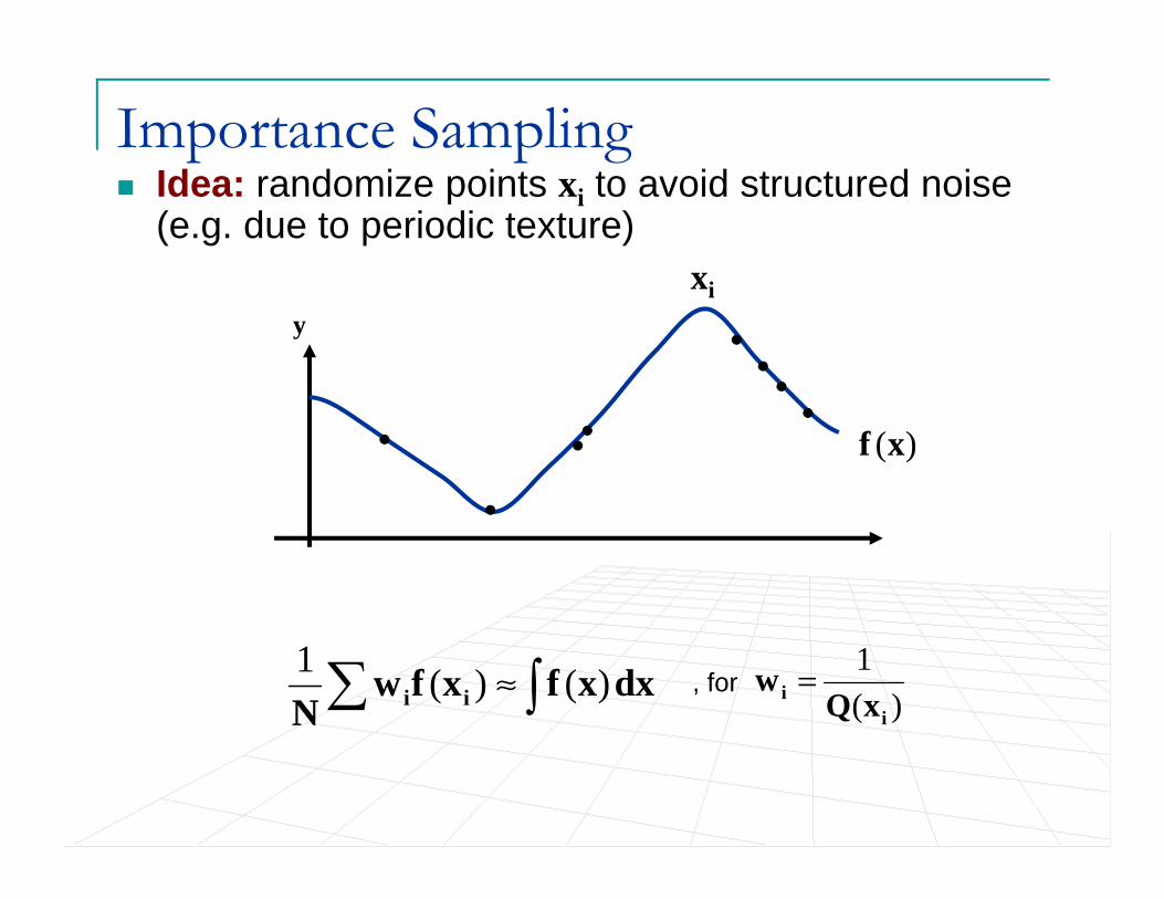
Importance SamplingIdea: randomize points xi to avoid structured noise (e.g. due to periodic texture)

xxiy

)(xf

∑ ∫≈ dxxfxfwN ii )()(1

)(1

ii xQ

w =, for

Shadows in Ray TracingRecall, we shoot a ray towards a light source and see if it is intercepted

knr

kp

jik dc ,

rr−=

knj

l

no shadow rays one shadow rayImages from the slides by Durand and Cutler

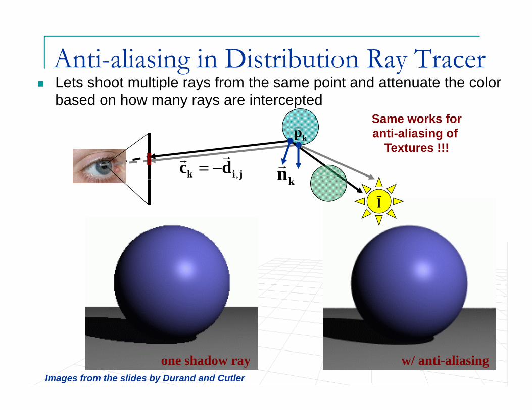
Anti-aliasing in Distribution Ray TracerLets shoot multiple rays from the same point and attenuate the color based on how many rays are intercepted

Same works forkp

jik dc ,

rr−=

knr

anti-aliasing of Textures !!!

j

l

kn

Images from the slides by Durand and Cutler

w/ anti-aliasingone shadow ray

Anti-aliasing by Deterministic IntegrationIdea: Use multiple rays for every pixel

Al ithAlgorithmSubdivide pixel (i,j) into squaresCast ray through square centersAverage the obtained light

Susceptible to structured noise, repeating texturesp , p g

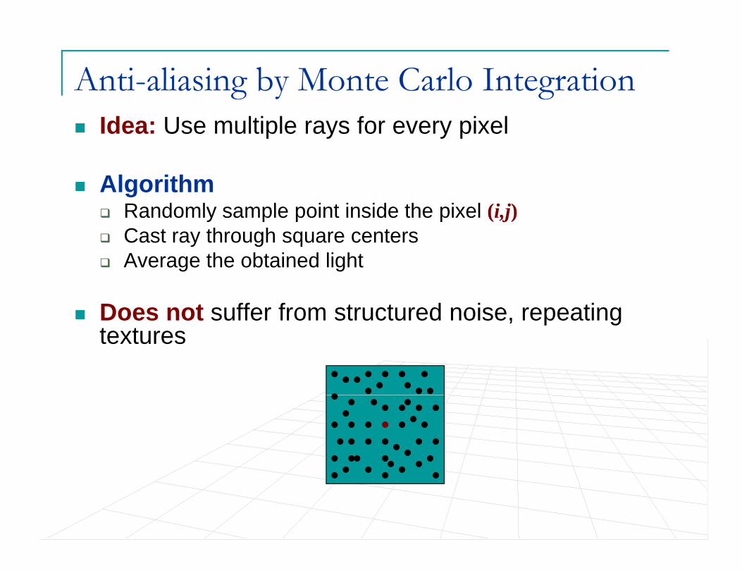
Anti-aliasing by Monte Carlo IntegrationIdea: Use multiple rays for every pixel

Al ithAlgorithmRandomly sample point inside the pixel (i,j)Cast ray through square centersAverage the obtained light

Does not suffer from structured noise, repeating , p gtextures

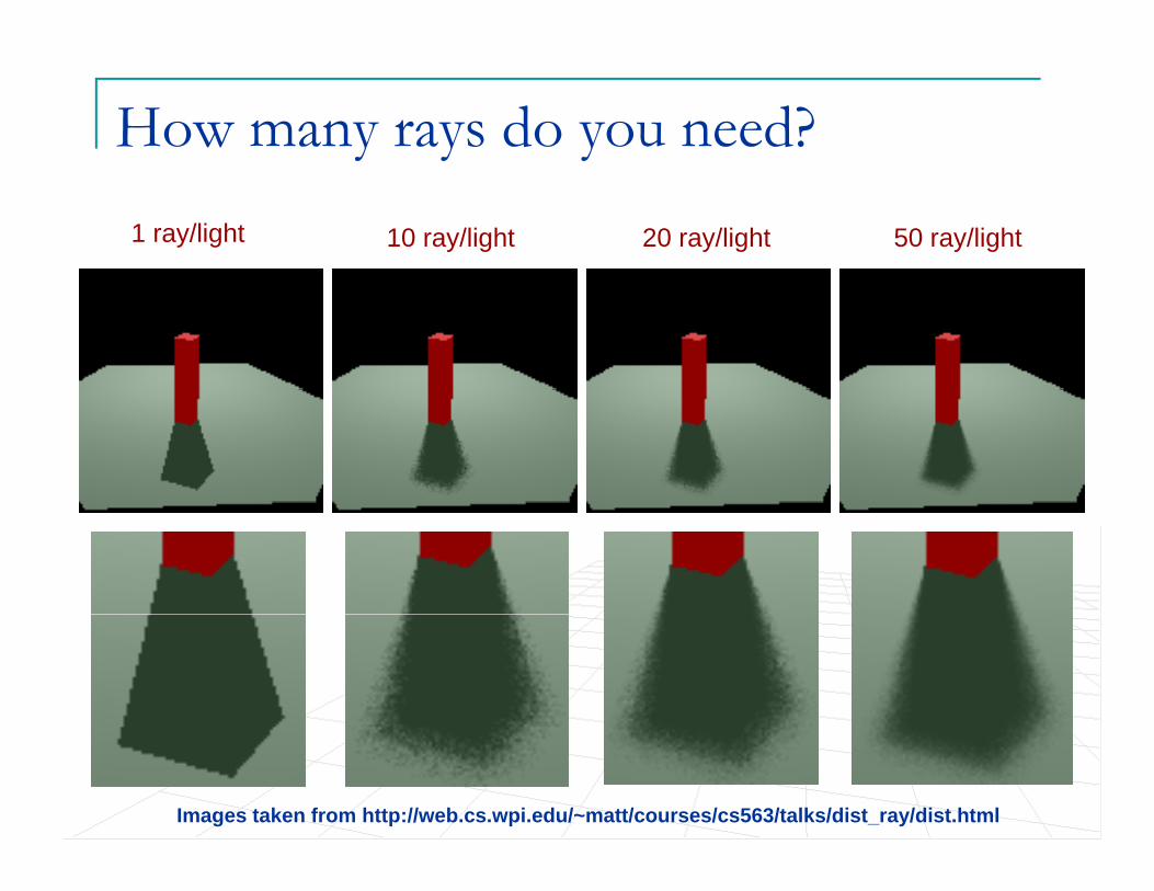
How many rays do you need?1 ray/light 10 ray/light 20 ray/light 50 ray/light

Images taken from http://web.cs.wpi.edu/~matt/courses/cs563/talks/dist_ray/dist.html

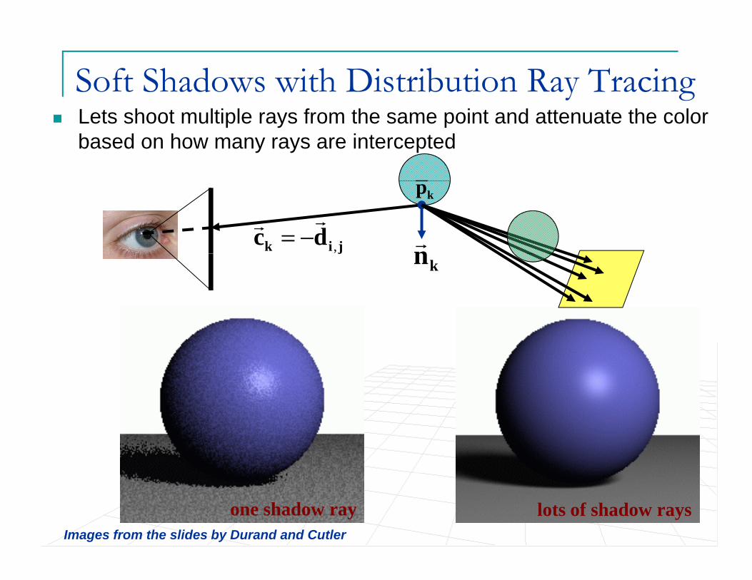
Soft Shadows with Distribution Ray TracingLets shoot multiple rays from the same point and attenuate the color based on how many rays are intercepted

nr

kp

jik dc ,

rr−=

knj

one shadow ray lots of shadow raysImages from the slides by Durand and Cutler

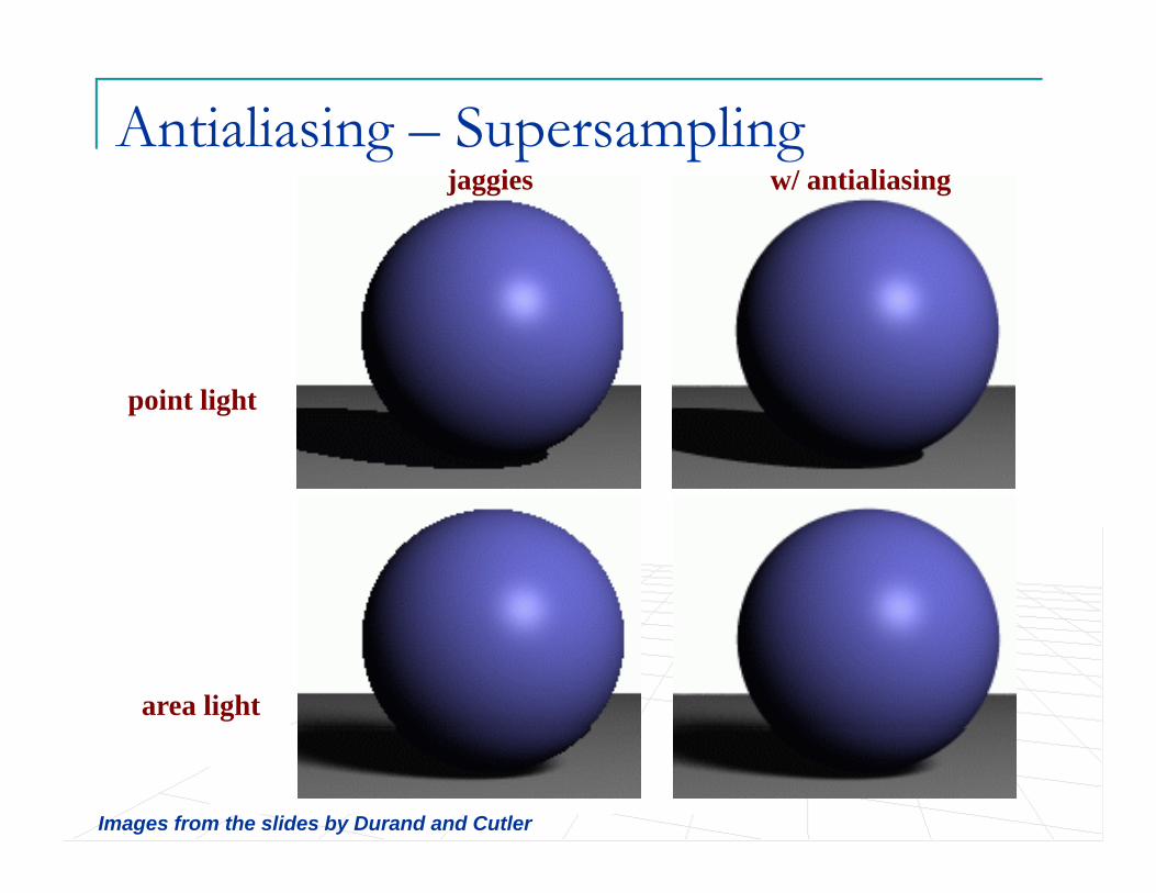
Antialiasing – Supersamplingjaggies w/ antialiasing

i li hpoint light

area light

Images from the slides by Durand and Cutler

Specular ReflectionsRecall, we had to shoot a ray in a perfect specular reflection direction (with respect to the camera) and get th di t th lti hit i tthe radiance at the resulting hit point

kpkkkks cnncm rrrrr

−⋅= )(2

knrjik dc ,

rr−=

ksr

kkkkk snnsrrrrrr

−⋅= )(2

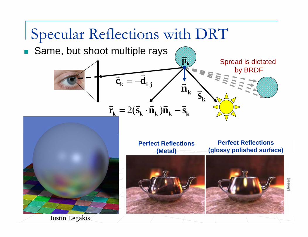
Specular Reflections with DRT

kpSame, but shoot multiple rays

Spread is dictated by BRDF

knrjik dc ,

rr−=

ksr

y

kkkkk snnsrrrrrr

−⋅= )(2

Perfect Reflections(Metal)

Perfect Reflections(glossy polished surface)

Justin Legakis

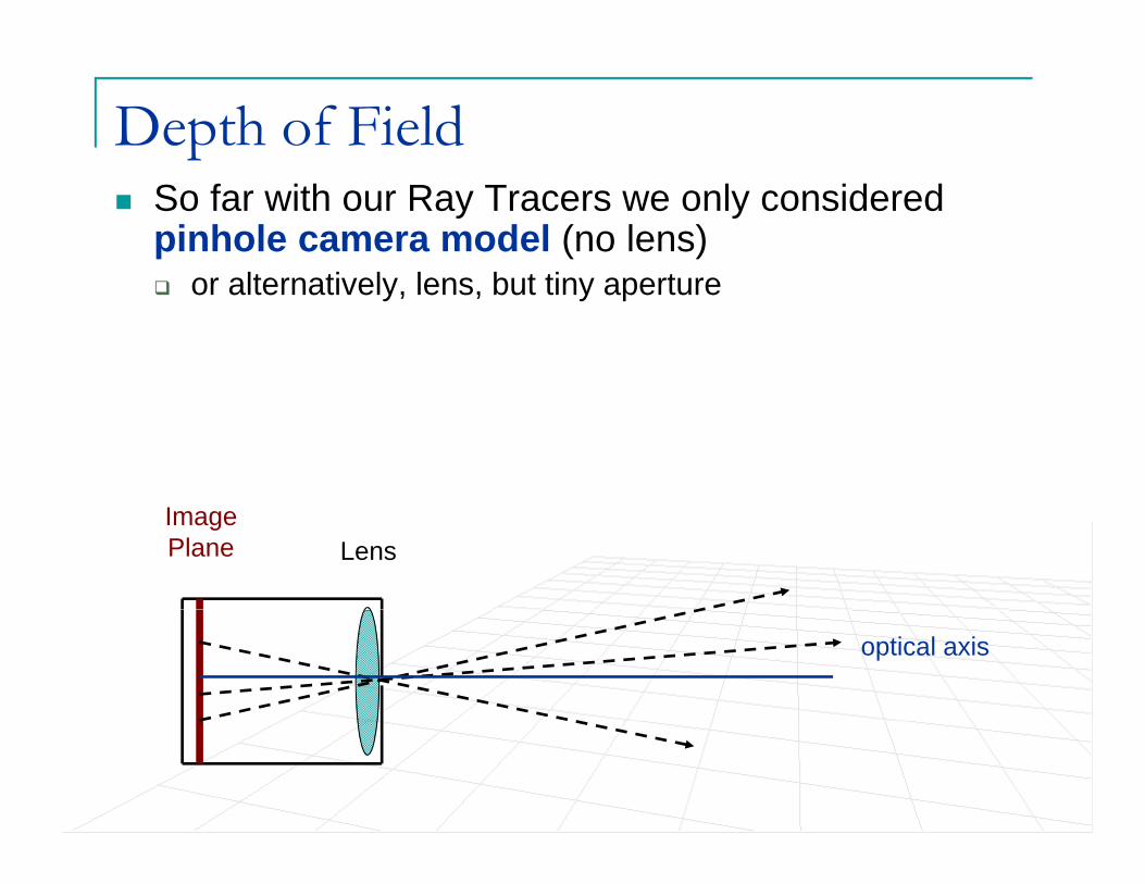
Depth of FieldSo far with our Ray Tracers we only considered pinhole camera model (no lens)

lt ti l l b t ti tor alternatively, lens, but tiny aperture

ImagePlane Lens

optical axis

Depth of FieldSo far with our Ray Tracers we only considered pinhole camera model (no lens)

lt ti l l b t ti tor alternatively, lens, but tiny apertureWhat happens if we put a lens into our “camera”

or increase the apertureo c ease t e ape tu eRemember the thin lens equation?

111ImagePlane Lens 10

111zzf

+=

optical axis

0z 1z

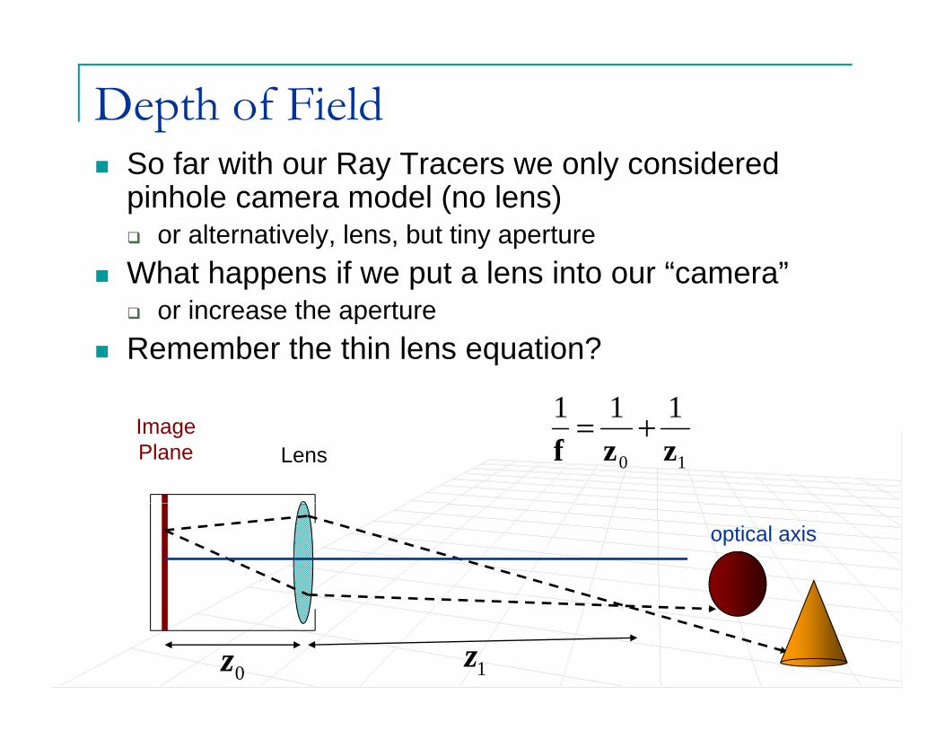
Depth of FieldSo far with our Ray Tracers we only considered pinhole camera model (no lens)

lt ti l l b t ti tor alternatively, lens, but tiny apertureWhat happens if we put a lens into our “camera”

or increase the apertureo c ease t e ape tu eRemember the thin lens equation?

111ImagePlane Lens 10

111zzf

+=

optical axis

0z 1z

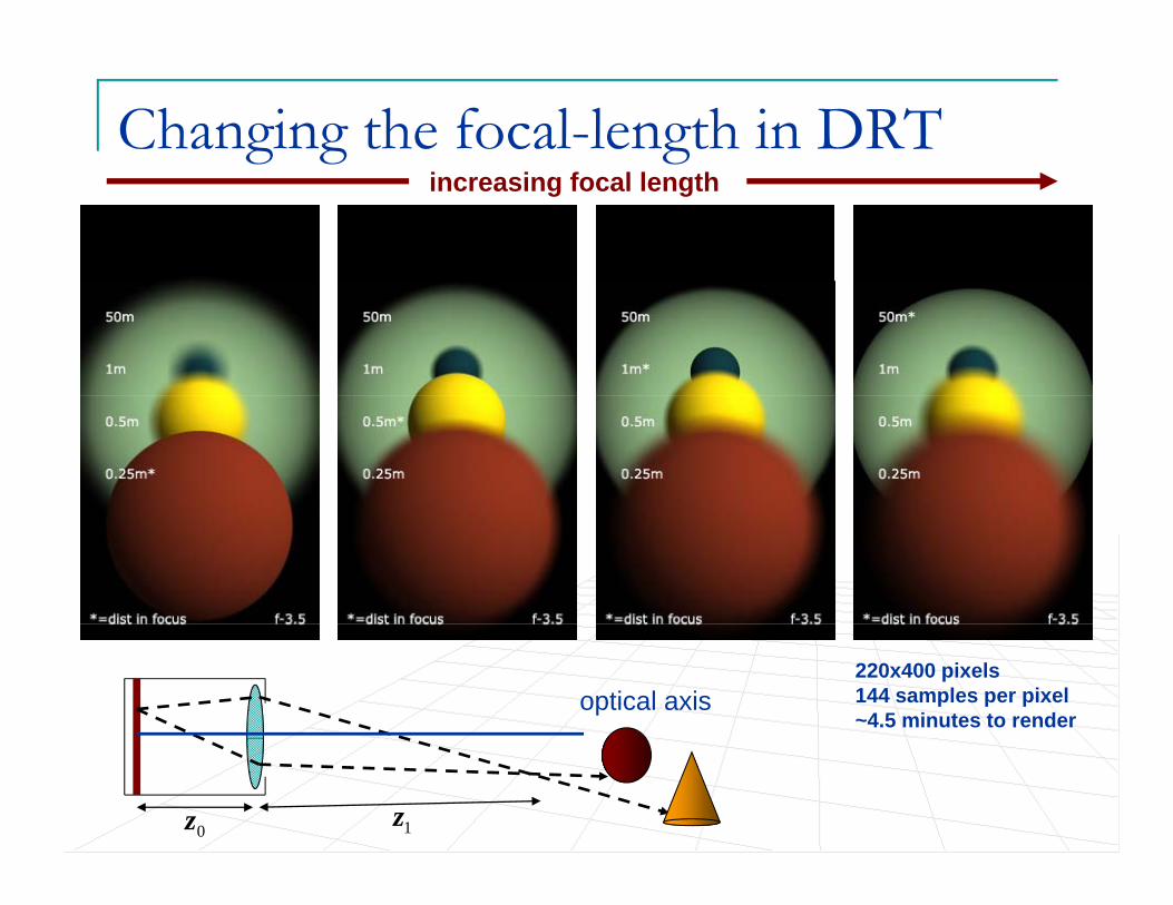
Changing the focal-length in DRTincreasing focal length

optical axis220x400 pixels144 samples per pixel~4.5 minutes to render

0z 1z

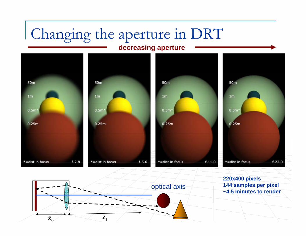
Changing the aperture in DRTdecreasing aperture

optical axis220x400 pixels144 samples per pixel~4 5 minutes to render

0z 1z

4.5 minutes to render

Depth of Field

Depth of Field

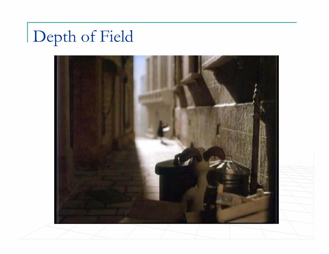
Depth of Field

Depth of Field

Depth of Field

Camera Shutter

We ignored the fact that it takes time to form the imageWe ignored the fact that it takes time to form the imageWe ignored this for radiometry

During that time the shutter is open and light is collectedWe need to integrate temporally, not only spatially

dtddtHt

βαβαα β

),,(∫ ∫ ∫

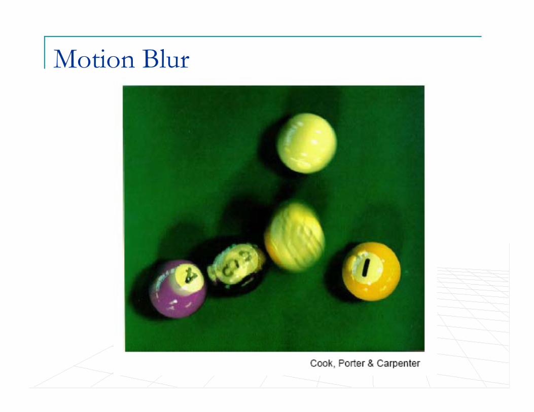
Motion Blur

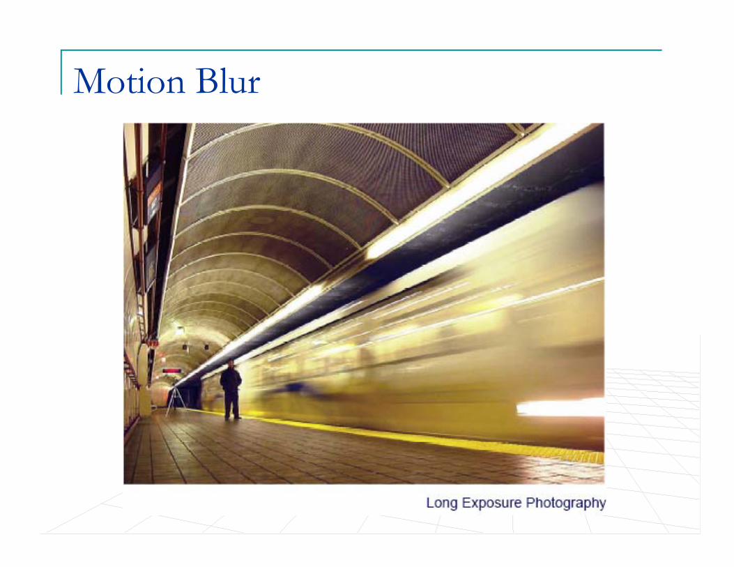
Motion Blur

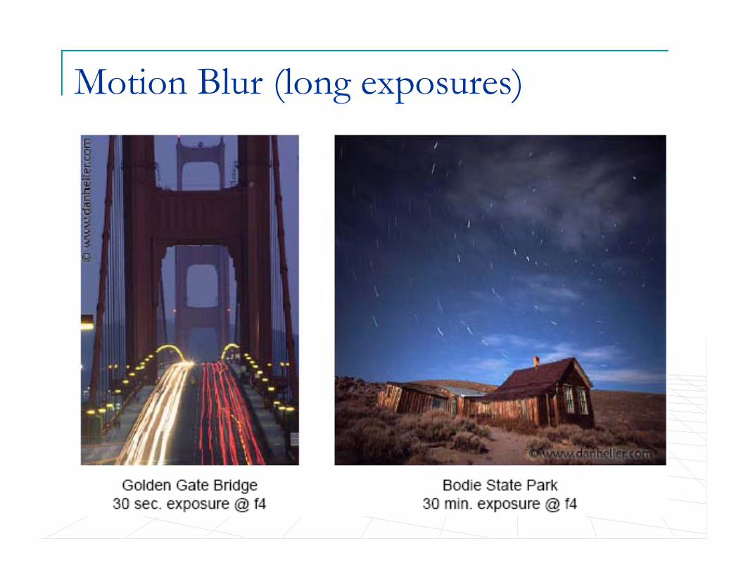
Motion Blur (long exposures)

Motion Blur (short exposures)

Sub-surface Scattering

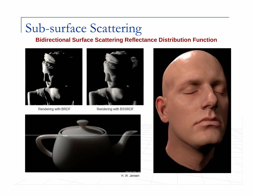
Sub-surface ScatteringBidirectional Surface Scattering Reflectance Distribution Function

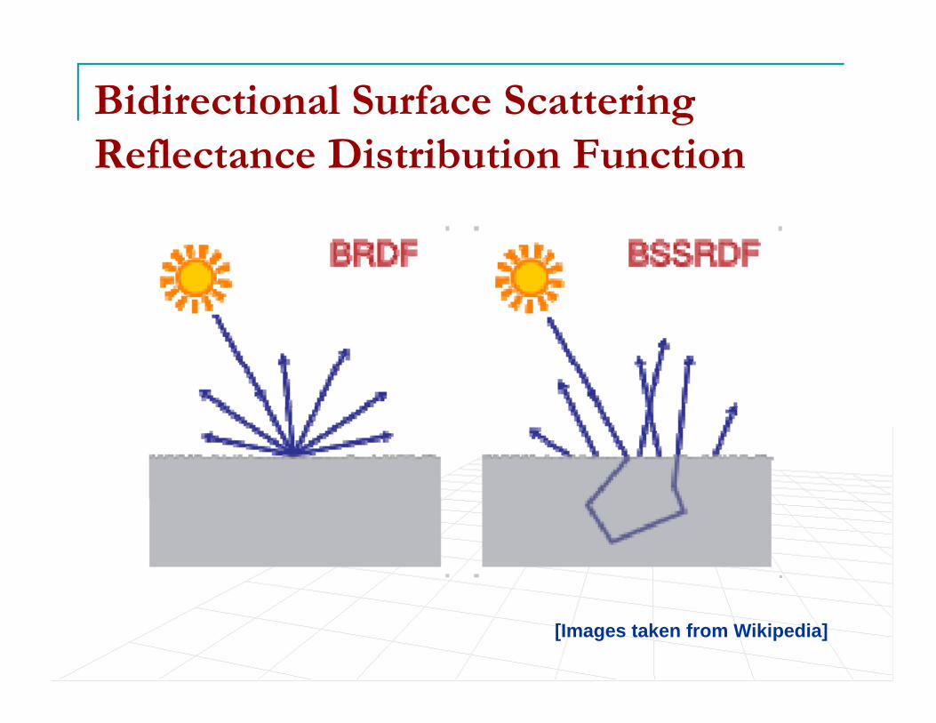
Bidirectional Surface Scattering Reflectance Distribution Function

[Images taken from Wikipedia]

Semi-Transparencies

Image form http://www.graphics.cornell.edu/online/tutorial/raytrace/

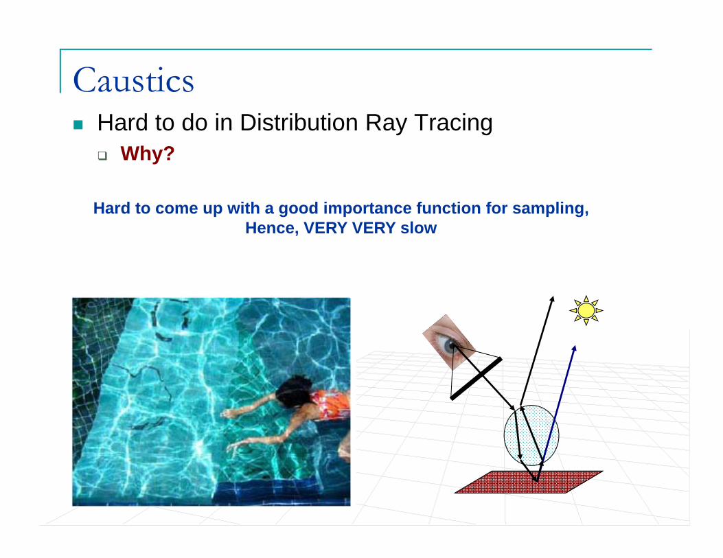
CausticsHard to do in Distribution Ray Tracing

Why?

CausticsHard to do in Distribution Ray Tracing

Why?

Hard to come up with a good importance function for sampling,Hence, VERY VERY slow

CausticsOften done using bi-directional ray tracing (a.k.a. photon mapping)

Shoot light rays from light sourcesShoot light rays from light sources Accumulate the amount of light (radiance) at each surfaceShoot rays through image plane pixels to “look-up” the

di ( d i t t i di th f thradiance (and integrate irradiance over the area of the pixel)

Photon Mapping

Simulates individual photonsSimulates individual photonsIn DTR we were simulating radiance (flux)

Photons are emitted from light sourcesPhotons are emitted from light sourcesPhotons bounce off of specular surfacesPh t d it d diff fPhotons are deposited on diffuse surfaces

Held in a 3-D spatial data structureS f d t b t i dSurfaces need not be parameterized

Photons collected by ray tracing from eye

PhotonsA photon is a particle of light that carries flux, which is encoded as follows

magnitude (in Watts) and color of the flux it carries, stored as an RGB triplelocation of the photon (on a diffuse surface)location of the photon (on a diffuse surface)the incident direction (used to compute irradiance)

E l ( i t li ht h t itt dExample (point light source, photons emitted uniformly)

Power of source (in Watts) distributed evenly among photons( ) y g pFlux of each photon equal to source power divided by total # of photons60W light bulb would sending 100 photons, will result in 0.660W light bulb would sending 100 photons, will result in 0.6 W per photon

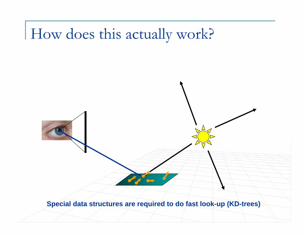
How does this actually work?

Special data structures are required to do fast look-up (KD-trees)

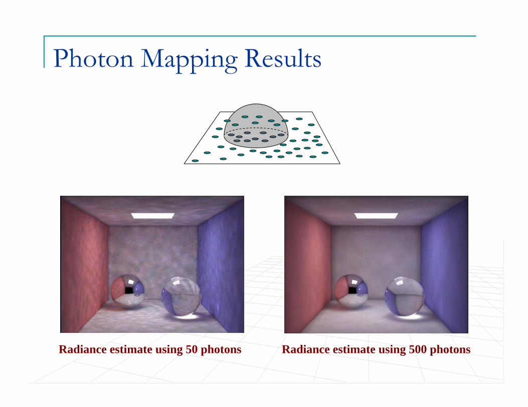
Photon Mapping Results

Radiance estimate using 50 photons Radiance estimate using 500 photons