WP/13/195

Distributional Consequences of Fiscal

Consolidation and the Role of Fiscal Policy:

What Do the Data Say?

Jaejoon Woo, Elva Bova, Tidiane Kinda,

and Y. Sophia Zhang

© 2013 International Monetary Fund WP/13/195

IMF Working Paper

Fiscal Affairs Department

Distributional Consequences of Fiscal Consolidation and the Role of Fiscal Policy:

What Do the Data Say?*

Prepared by Jaejoon Woo, Elva Bova, Tidiane Kinda, and Y. Sophia Zhang

Authorized for Distribution by Martine Guerguil

September 2013

Abstract

The 2007-09 Great Recession has led to an unprecedented increase in public debt in many

countries, triggering substantial fiscal adjustments. What are the distributional consequences of

fiscal austerity measures? This is an important policy question. This paper analyzes the effects of

fiscal policies on income inequality in a panel of advanced and emerging market economies over

the last three decades, complemented by a case study of selected consolidation episodes. The

paper shows that fiscal consolidations are likely to raise inequality through various channels

including their effects on unemployment. Spending-based consolidations tend to worsen

inequality more significantly, relative to tax-based consolidations. The composition of austerity

measures also matters: progressive taxation and targeted social benefits and subsidies introduced

in the context of a broader decline in spending can help offset some of the adverse distributional

impact of consolidation. In addition, fiscal policy can favorably influence long-term trends in

both inequality and growth by promoting education and training among low- and middle-income

workers.

JEL Classification Numbers: D30, D63, H20, I24, I38

Keywords: Inequality, Gini Coefficient, Fiscal Consolidation, Fiscal Policy, Tax and Spending policy

Authors’ E-Mail Addresses: jwoo@imf.org; ebova@imf.org; tkinda@imf.org; yzhang@imf.org

* The authors would like to thank Martin Cerisola, David Coady, Carlo Cottarelli, Xavier Debrun, Markus Eller,

Greetje Everaert, Lorenzo Forni, Davide Furceri, Phil Gerson, Martine Guerguil, Sanjeev Gupta, Mulas

Granados, Frigyes Heinz, Andrea Lemgruber, Laura Jaramillo Mayor, Leandro Medina, Tigran Poghosyan,

Marcos Poplawski Ribeiro, Serges Saksonovs, Andrea Schaechter, Bahrom Shukurov, Yan Sun, Anke Weber,

and participants in IMF seminars and Villa Mondragone International Economic Seminar in Rome for helpful

comments and discussions. The main results of the paper were published in the IMF’s October 2012 Fiscal

Monitor. Petra Dacheva and Carsten Jung provided excellent research assistance.

This Working Paper should not be reported as representing the views of the IMF.

The views expressed in this Working Paper are those of the author(s) and do not necessarily represent those of

the IMF or IMF policy. Working Papers describe research in progress by the author(s) and are published to

elicit comments and to further debate.

1

Contents Page

I. Introduction ....................................................................................................................2

II. Data, Trends In Income Distribution, and Related Studies ...........................................4

III. Econometric Analysis: Fiscal Consolidation, Fiscal Policy, and Inequality .................8

IV. Case Study of Fiscal Consolidation Episodes ..............................................................18

V. Concluding Remarks ....................................................................................................20

Tables

1. Pairwise Correlation of Measures of Income Distribution and

Unemployment, 1980-2010 .........................................................................................26

2. Impact on Disposable Income Gini Coefficient of Fiscal Consolidation:

OECD Countries, 1978-2009 .......................................................................................27

3. Determinants of Income Inequality, 1980-2010 ..................................................................28

Box

1. Fiscal Policy and Inequality: Survey of Evidence .................................................................8

Figures

1. Selected European Economies: Change in ..........................................................................21

2. Trends in Disposable Income Inequality: Gini Coefficient, 1985-2010 ..............................22

3. Ratio of Direct to Indirect Taxes and Social Benefits Spending, 1980-2009 ......................23

4. Dynamic Effects of Fiscal Consolidation on Income ..........................................................24

5. Changes in Income Inequality: Spending-Based versus Tax-Based ....................................25

Appendixes

1. Description of Data and List of Sample Countries ..............................................................30

Appendix Tables

1. Level of Initial Government Debt, Growth, and Investment, 1970–2007 ...........................31

2. Cross-country Regression—Government Debt and Real per capita GDP Growth .............31

References ................................................................................................................................32

2

I. INTRODUCTION

The Great Recession of 2007-09 has led to an unprecedented increase in public debt, raising

serious concerns about fiscal sustainability. Against this backdrop, many governments have

been making substantial fiscal adjustments through a combination of spending cuts and tax

hikes to reduce their ratios of debt to GDP. What are the distributional consequences of fiscal

austerity measures?1 This is an important policy question. Preventing a significant worsening

of income distribution during the adjustment period is critical to the sustainability of deficit

reduction efforts, as a consolidation that is perceived as being fundamentally unfair will be

difficult to maintain. Moreover, high income inequality can harm long-term growth through

various channels (for example, see Easterly 2007; Berg et al. 2011; and Woo 2011).2

Surprisingly, however, there has been little systematic analysis of the distributional effects of

fiscal consolidations.3

This paper provides evidence on the effects of fiscal consolidation and a set of fiscal

variables (tax structure, specific taxes and expenditures) on income inequality in a panel of

advanced and emerging market economies over the last three decades, which is

complemented with a case study of selected consolidation episodes. For the econometric

analysis, the paper builds on a large literature on the determinants of cross-country variations

in income inequality (for example, see De Gregorio and Lee 2002; IMF 2007; and Barro

2008).

Specifically, we address the following two sets of questions: (i) Does fiscal austerity worsen

income inequality? If so, how and by how much? Does the size of fiscal adjustment matter?

(ii) What are the effects on income distribution of specific fiscal policies, such as tax

structure, direct and indirect taxes, social benefits spending and wage bills? Exploring the

latter would provide some guidance on adjustment packages that would limit their adverse

effects, if any, on inequality. Our results suggest that fiscal consolidations tend to increase

income inequality, including through their effects on unemployment. Alternative estimation

methods find a similar range of impact magnitude: on average, a consolidation of 1

1 The distributional impact of failing to adjust is beyond the scope of the paper. However, the impact on income

distribution of a delay in fiscal consolidation could be even worse if it results in an eventual debt crisis that

forces a sudden, even greater fiscal adjustment, accompanied by a severe recession.

2 The paper focuses on the distributional effects of fiscal adjustments and of fiscal policy, but it is important to

recognize the potential trade-off between equity and efficiency when designing redistributive policies.

Redistributive tax and benefit systems can introduce economic efficiencies with implications for long-term

productivity and growth, as redistributive policies can influence the incentives for people to work, save and

invest. There is a large literature on the relationship between inequality and growth (besides the aforementioned

papers, see also Alesina and Rodrik 1994; Banerjee and Duflo 2003; Bertola et al. 2005; and Barro 2008 and

references therein).

3 Notable exceptions are Agnello and Sousa (2012) for 18 OECD countries in 1978-2009 and Mulas-Granados

(2005) for 15 EU nations in 1960-2000.

3

percentage point of GDP is associated with an increase in the disposable income Gini

coefficient of around 0.4-0.7 percent over the first two years. Spending-based consolidations

tend to significantly worsen inequality, relative to tax-based consolidations. So do large-sized

consolidations (those greater than 1½ percent of GDP). This seems to reflect the fact that

large-sized consolidations tend to be longer in duration and mostly expenditure-based, which

is confirmed in the case study. Unemployment also tends to increase inequality, and hence, to

the extent that fiscal consolidation raises unemployment, it constitutes an important channel

through which consolidation affects inequality. Loosely speaking, about 15-20 percent of the

increase in inequality due to consolidation may be occurring via the increase in

unemployment.

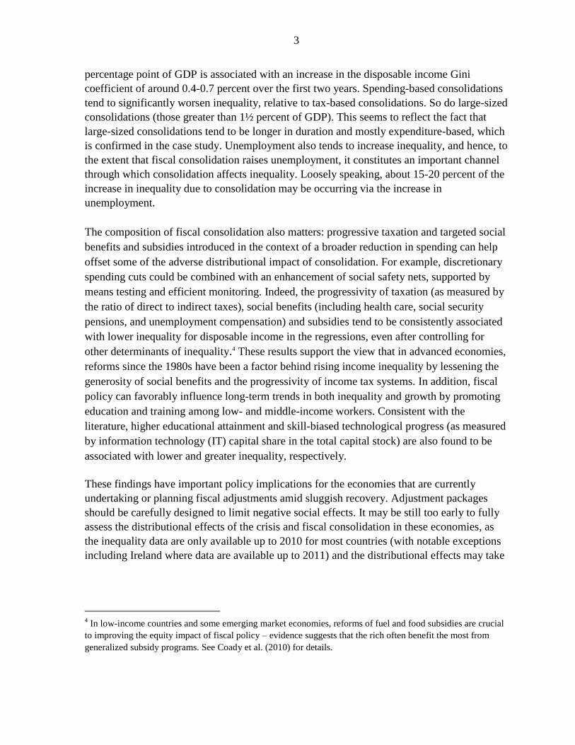
The composition of fiscal consolidation also matters: progressive taxation and targeted social

benefits and subsidies introduced in the context of a broader reduction in spending can help

offset some of the adverse distributional impact of consolidation. For example, discretionary

spending cuts could be combined with an enhancement of social safety nets, supported by

means testing and efficient monitoring. Indeed, the progressivity of taxation (as measured by

the ratio of direct to indirect taxes), social benefits (including health care, social security

pensions, and unemployment compensation) and subsidies tend to be consistently associated

with lower inequality for disposable income in the regressions, even after controlling for

other determinants of inequality.4 These results support the view that in advanced economies,

reforms since the 1980s have been a factor behind rising income inequality by lessening the

generosity of social benefits and the progressivity of income tax systems. In addition, fiscal

policy can favorably influence long-term trends in both inequality and growth by promoting

education and training among low- and middle-income workers. Consistent with the

literature, higher educational attainment and skill-biased technological progress (as measured

by information technology (IT) capital share in the total capital stock) are also found to be

associated with lower and greater inequality, respectively.

These findings have important policy implications for the economies that are currently

undertaking or planning fiscal adjustments amid sluggish recovery. Adjustment packages

should be carefully designed to limit negative social effects. It may be still too early to fully

assess the distributional effects of the crisis and fiscal consolidation in these economies, as

the inequality data are only available up to 2010 for most countries (with notable exceptions

including Ireland where data are available up to 2011) and the distributional effects may take

4 In low-income countries and some emerging market economies, reforms of fuel and food subsidies are crucial

to improving the equity impact of fiscal policy – evidence suggests that the rich often benefit the most from

generalized subsidy programs. See Coady et al. (2010) for details.

4

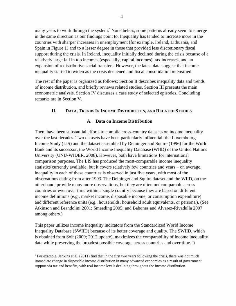
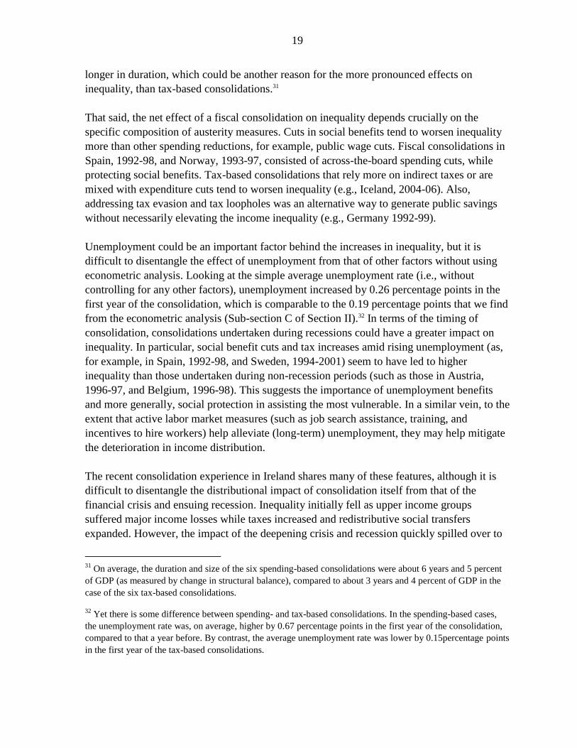
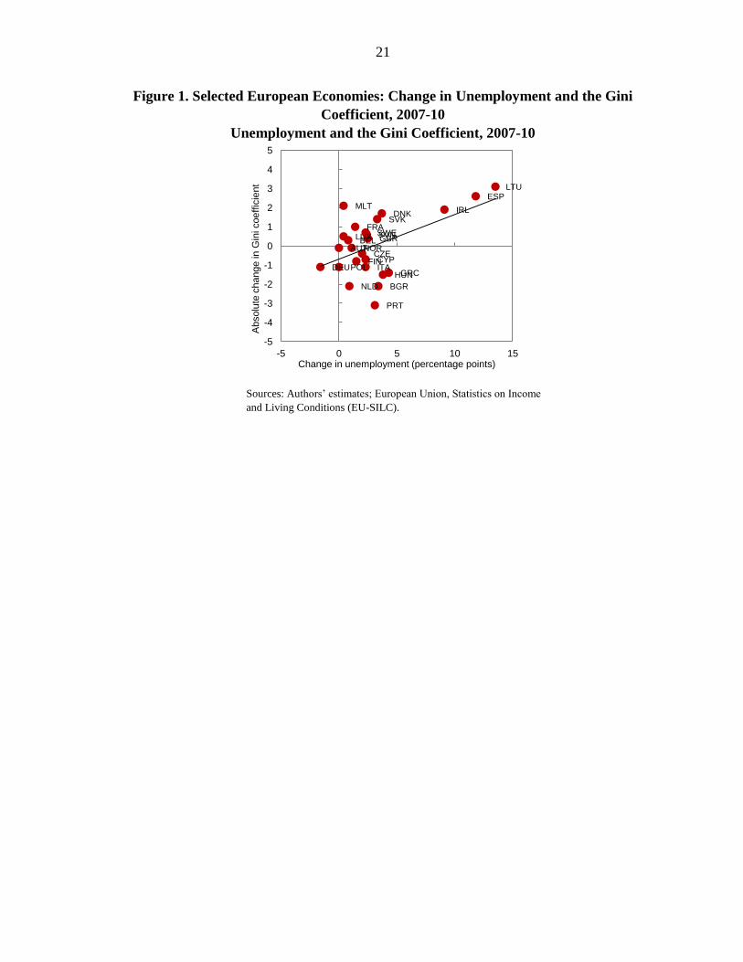
many years to work through the system.5 Nonetheless, some patterns already seem to emerge

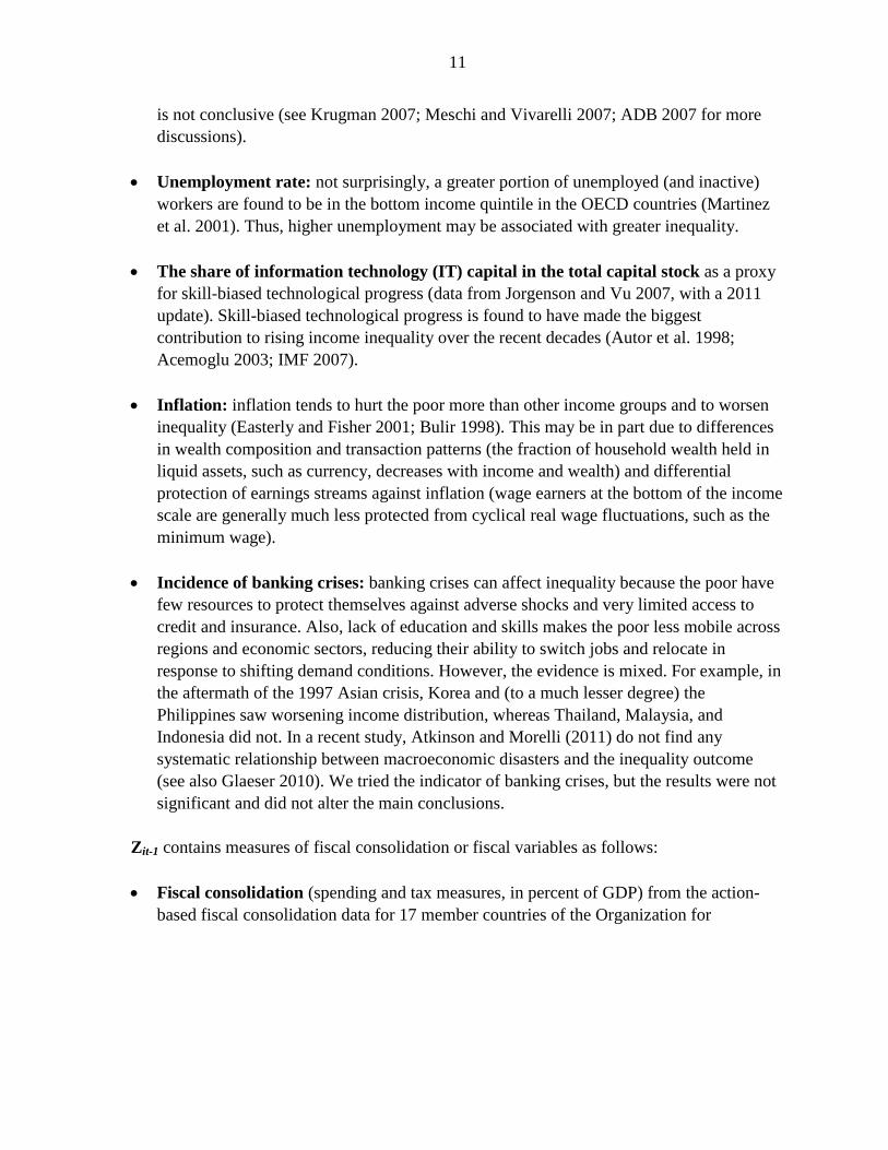
in the same direction as our findings point to. Inequality has tended to increase more in the

countries with sharper increases in unemployment (for example, Ireland, Lithuania, and

Spain in Figure 1) and to a lesser degree in those that provided less discretionary fiscal

support during the crisis. In Ireland, inequality initially declined during the crisis because of a

relatively large fall in top incomes (especially, capital incomes), tax increases, and an

expansion of redistributive social transfers. However, the latest data suggest that income

inequality started to widen as the crisis deepened and fiscal consolidation intensified.

The rest of the paper is organized as follows: Section II describes inequality data and trends

of income distribution, and briefly reviews related studies. Section III presents the main

econometric analysis. Section IV discusses a case study of selected episodes. Concluding

remarks are in Section V.

II. DATA, TRENDS IN INCOME DISTRIBUTION, AND RELATED STUDIES

A. Data on Income Distribution

There have been substantial efforts to compile cross-country datasets on income inequality

over the last decades. Two datasets have been particularly influential: the Luxembourg

Income Study (LIS) and the dataset assembled by Deininger and Squire (1996) for the World

Bank and its successor, the World Income Inequality Database (WIID) of the United Nations

University (UNU-WIDER, 2008). However, both have limitations for international

comparison purposes. The LIS has produced the most-comparable income inequality

statistics currently available, but it covers relatively few countries and years – on average,

inequality in each of these countries is observed in just five years, with most of the

observations dating from after 1993. The Deininger and Squire dataset and the WIID, on the

other hand, provide many more observations, but they are often not comparable across

countries or even over time within a single country because they are based on different

income definitions (e.g., market income, disposable income, or consumption expenditure)

and different reference units (e.g., households, household adult equivalents, or persons,). (See

Atkinson and Brandolini 2001; Smeeding 2005; and Babones and Alvarez-Rivadulla 2007

among others.)

This paper utilizes income inequality indicators from the Standardized World Income

Inequality Database (SWIID) because of its better coverage and quality. The SWIID, which

is obtained from Solt (2009; 2012 update), maximizes the comparability of income inequality

data while preserving the broadest possible coverage across countries and over time. It

5 For example, Jenkins et al. (2011) find that in the first two years following the crisis, there was not much

immediate change in disposable income distribution in many advanced economies as a result of government

support via tax and benefits, with real income levels declining throughout the income distribution.

5

standardizes the WIID database and provides comparable Gini coefficients for market and

disposable income for up to 153 countries for as many years as possible from 1960 to 2011

(see Solt 2009 for details).

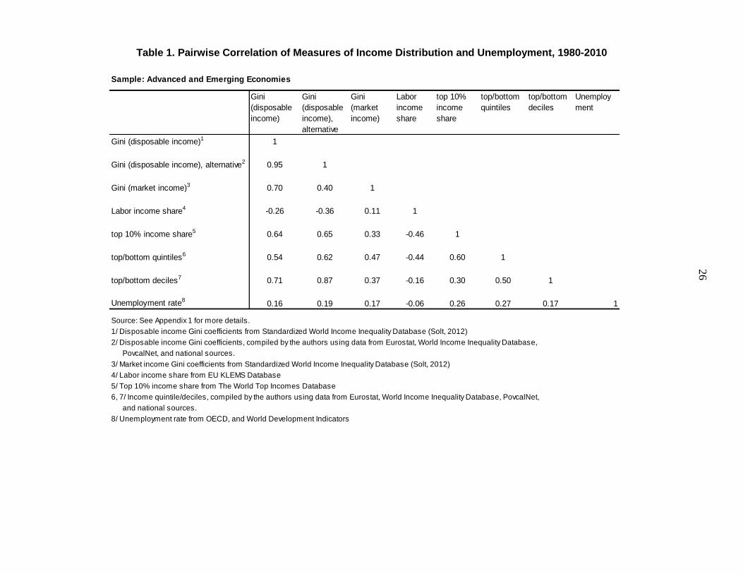
As further robustness checks, we use alternative data on Gini coefficients for disposable

income and alternative measures of income inequality (e.g., ratios of top to bottom

quintiles/deciles, and labor income share) compiled from original sources including the

WIID, the LIS, World Bank’s PovcalNet, and Eurostat. Measures of income inequality are

relatively highly correlated with each other (Table 1) – for example, the correlation

coefficient between Gini indices for disposable income from the SWIID and those in

alternative dataset compiled from the aforementioned original sources is 0.95 (p-value=0.00).

B. Trends in Income Inequality

Data suggest that income inequality has increased since the 1980s in most advanced and

many developing economies. This reflects an array of factors including skill-biased

technological progress, technology diffusion, international trade, and market reforms.

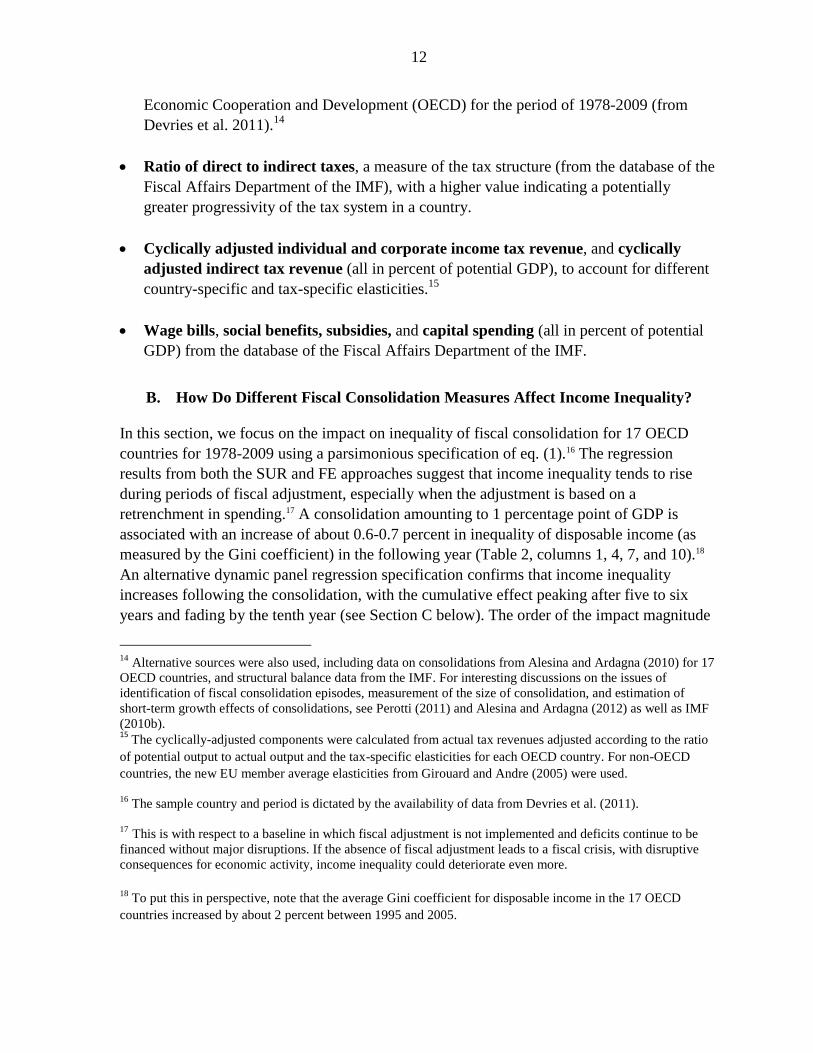
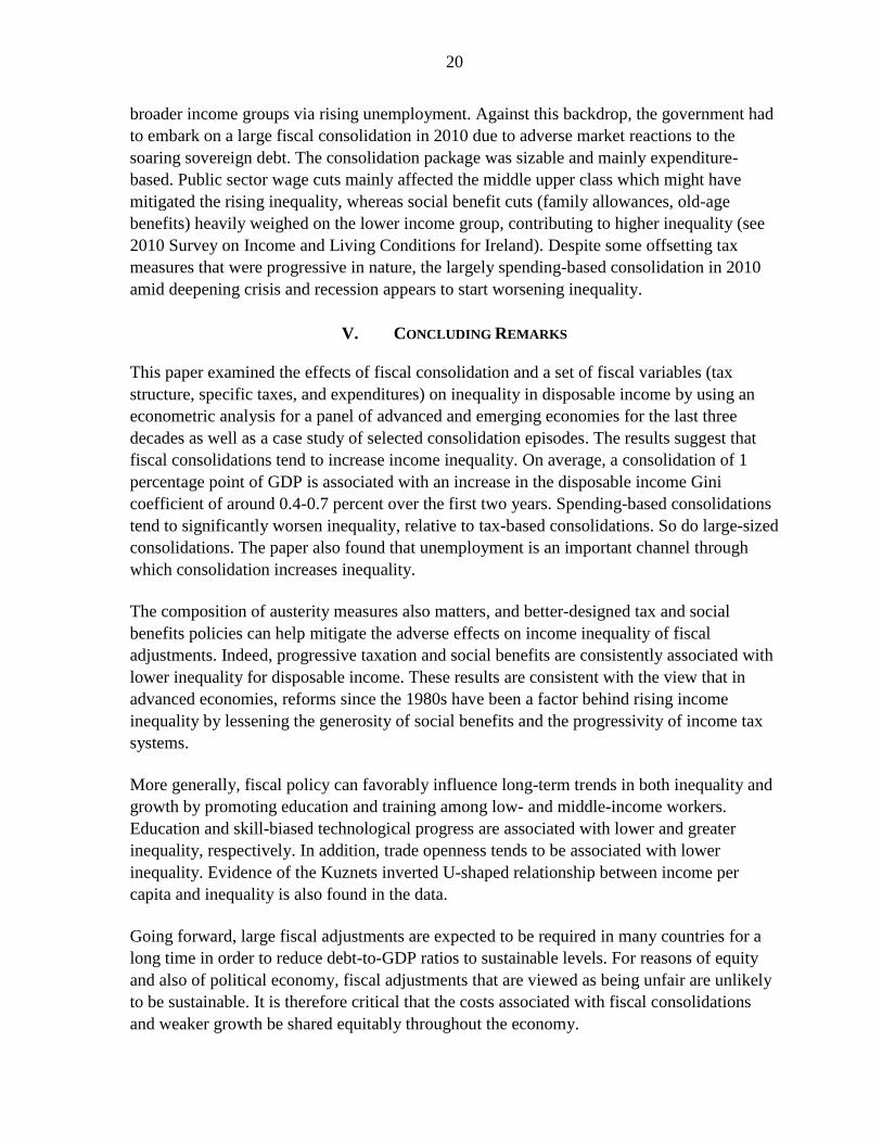
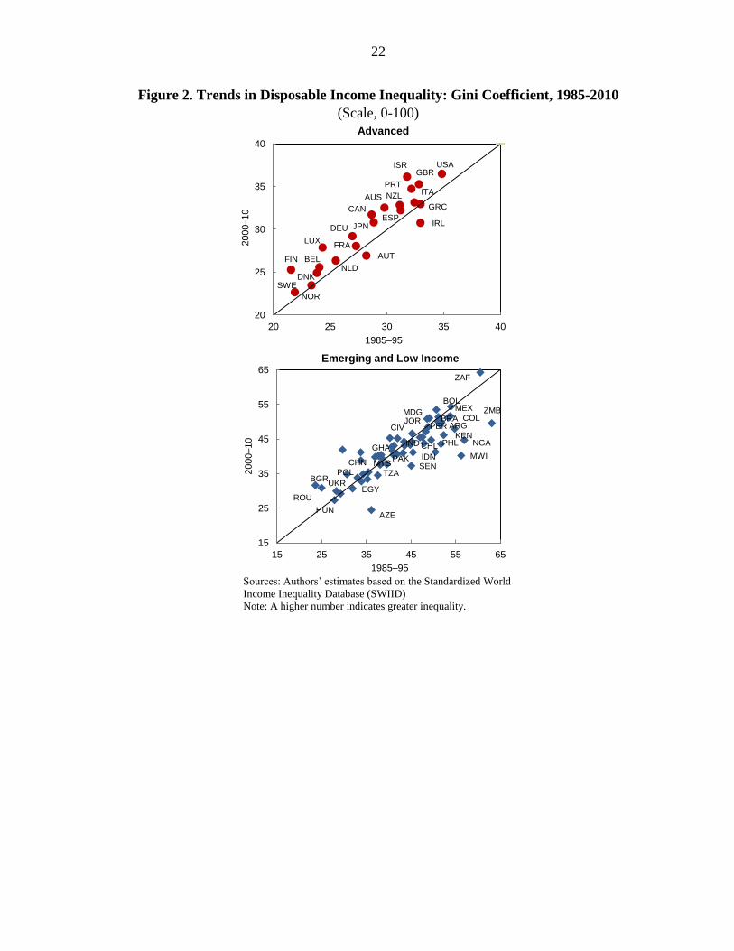
Inequality in disposable income (income after taxes and transfers) exhibits a similar upward

trend, but there is a wider variation across countries and regions, largely due to different

degrees of progressivity in income tax systems and spending policies (Figure 2).6

During 1980-2010, the average disposable income Gini coefficients in advanced economies

and emerging Europe, the most equal regions, increased by 3 and 6 percentage points,

respectively. The Gini coefficients also increased in most countries in Asia and the Pacific

region during the same period. In the two most unequal regions (Sub-Saharan Africa and

Latin America), however, income inequality increased in the 1980s and 1990s but

subsequently declined markedly.

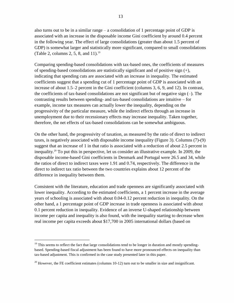
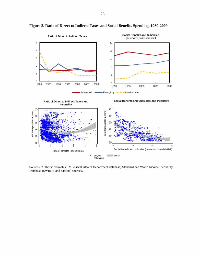
In advanced economies, redistributive fiscal policy has played a significant role in reducing

inequality in market income via progressive tax system and social transfers. However,

reforms since the 1980s have been a factor behind rising income inequality by lessening the

generosity of social benefits and the progressivity of income tax systems (Figure 3).

Consistent with this observation, the correlation coefficient between the Gini coefficient for

market income and that for disposable income has markedly declined from 0.5 in the 1990s

to 0.37 in the 2000s.

In emerging and low-income economies, the redistributive capacity of fiscal policy has

historically been limited because of weak taxation systems (large parts of the economy are

6 For a review of income inequality trends and evolution of fiscal policies, see Bastagli et al. (2012), Chu et al.

(2004) and references therein.

6

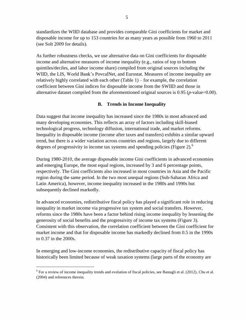
outside the income tax system, and the efficiency of tax collection is relatively low) and

poorly targeted social transfers (see Chu et al. 2004; Gemmell and Morrissey 2005; and

Box 1). Social benefits and subsidies increased in these countries since the 1980s. However,

their declining ratio of direct to indirect taxes indicates decreasing tax progressivity. Overall,

data point to a strong negative association between social spending and disposable income

inequality and to a negative, albeit less clear cut, relationship between the ratio of direct to

indirect taxes and inequality in the entire sample of advanced, emerging and low-income

economies for the period of 1980-2009.

Box 1. Fiscal Policy and Inequality: A Survey of Evidence

Authors Period

1970-2009

Joumard et al. 2012

Paulus et al. 2009 mid-2000s

Chu et al. 2000 1970s-1990s

1960s-90s

Cubero & Hollar 2010 1995-2008

Lorenz and

concentration curves;

six African countries

From literature review and their estimation: personal income

taxes are progressive, corporate taxes have a U-shape effect

(regressive and then progressive); property, indirect taxes

and taxes on exports are regressive. Overall tax systems are

regressive at low income levels.

Redistributive policy is more effective in Europe than in Latin

America. In both regions, redistribution is more effective

through transfers than taxes.

Lorenz &

concentration curves,

quasi-Gini coefficients,

Kakwani and Reynolds-

Smolensky indexes;

Cental America.

Income taxes are progressive; VAT, sales taxes, excise

duties and international trade taxes are regressive. Social

security spending is regressive, while total education and

health spending are progressive. Social spending has a more

redistributive potential than taxes.

Market and disposable-

income Gini; Latin

America and Western

Europe.

Different

selected

years

Progressive PIT & CIT reduce inequality (for CIT, smaller

effect with more globalization). Consumption taxes, excises,

customs duties increase inequality. Welfare, education,

health, and housing expenditures reduce inequality.

Market- and disposable-

income Gini; OECD

countries.

mid 1990s-

late 2000s

Transfers reduce income dispersion more than taxes. Family

and housing benefits are the most progressive while pension

benefits the most regressive. Income taxes are the most

progressive; while, consumption and real estate taxes the

most regressive.

Inequality measure

& country sampleEmpirical findings

Martinez-Vazquez et

al. 2012

Gemmell & Morrissey

2005

Goni, Lopez & Serven

2008

Fiscal policies and inequality

Gini coefficients,

deciles; 19 European

Union countries.

Benefits and personal taxes have the largest redistributive

impact; social contributions smallest impact. In Scandinavia,

Austria & Belgium, non means-tested benefits have a larger

impact; while in Ireland and the UK, means-tested benefits

have a larger impact.

Gini coefficients; 19

developing countries

From literature review and their estimation: less unequal

before-tax distribution in developing countries than in OECD;

smaller tax redistributive effect. Income tax, health and

education spending are progressive. Direct/indirect tax

change is progressive.

Gini coefficients; 150

countries.

7

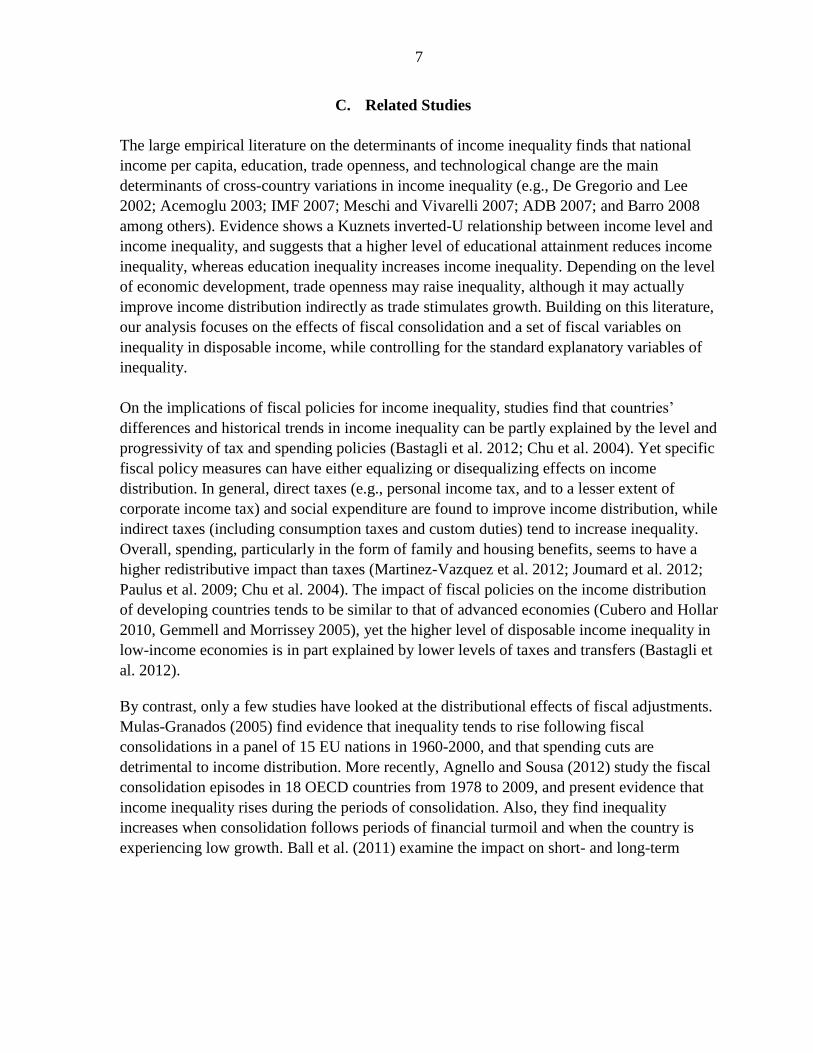
C. Related Studies

The large empirical literature on the determinants of income inequality finds that national

income per capita, education, trade openness, and technological change are the main

determinants of cross-country variations in income inequality (e.g., De Gregorio and Lee

2002; Acemoglu 2003; IMF 2007; Meschi and Vivarelli 2007; ADB 2007; and Barro 2008

among others). Evidence shows a Kuznets inverted-U relationship between income level and

income inequality, and suggests that a higher level of educational attainment reduces income

inequality, whereas education inequality increases income inequality. Depending on the level

of economic development, trade openness may raise inequality, although it may actually

improve income distribution indirectly as trade stimulates growth. Building on this literature,

our analysis focuses on the effects of fiscal consolidation and a set of fiscal variables on

inequality in disposable income, while controlling for the standard explanatory variables of

inequality.

On the implications of fiscal policies for income inequality, studies find that countries’

differences and historical trends in income inequality can be partly explained by the level and

progressivity of tax and spending policies (Bastagli et al. 2012; Chu et al. 2004). Yet specific

fiscal policy measures can have either equalizing or disequalizing effects on income

distribution. In general, direct taxes (e.g., personal income tax, and to a lesser extent of

corporate income tax) and social expenditure are found to improve income distribution, while

indirect taxes (including consumption taxes and custom duties) tend to increase inequality.

Overall, spending, particularly in the form of family and housing benefits, seems to have a

higher redistributive impact than taxes (Martinez-Vazquez et al. 2012; Joumard et al. 2012;

Paulus et al. 2009; Chu et al. 2004). The impact of fiscal policies on the income distribution

of developing countries tends to be similar to that of advanced economies (Cubero and Hollar

2010, Gemmell and Morrissey 2005), yet the higher level of disposable income inequality in

low-income economies is in part explained by lower levels of taxes and transfers (Bastagli et

al. 2012).

By contrast, only a few studies have looked at the distributional effects of fiscal adjustments.

Mulas-Granados (2005) find evidence that inequality tends to rise following fiscal

consolidations in a panel of 15 EU nations in 1960-2000, and that spending cuts are

detrimental to income distribution. More recently, Agnello and Sousa (2012) study the fiscal

consolidation episodes in 18 OECD countries from 1978 to 2009, and present evidence that

income inequality rises during the periods of consolidation. Also, they find inequality

increases when consolidation follows periods of financial turmoil and when the country is

experiencing low growth. Ball et al. (2011) examine the impact on short- and long-term

8

effects on unemployment of fiscal adjustments and find evidence that unemployment tends to

rise following adjustments in advanced economies.7

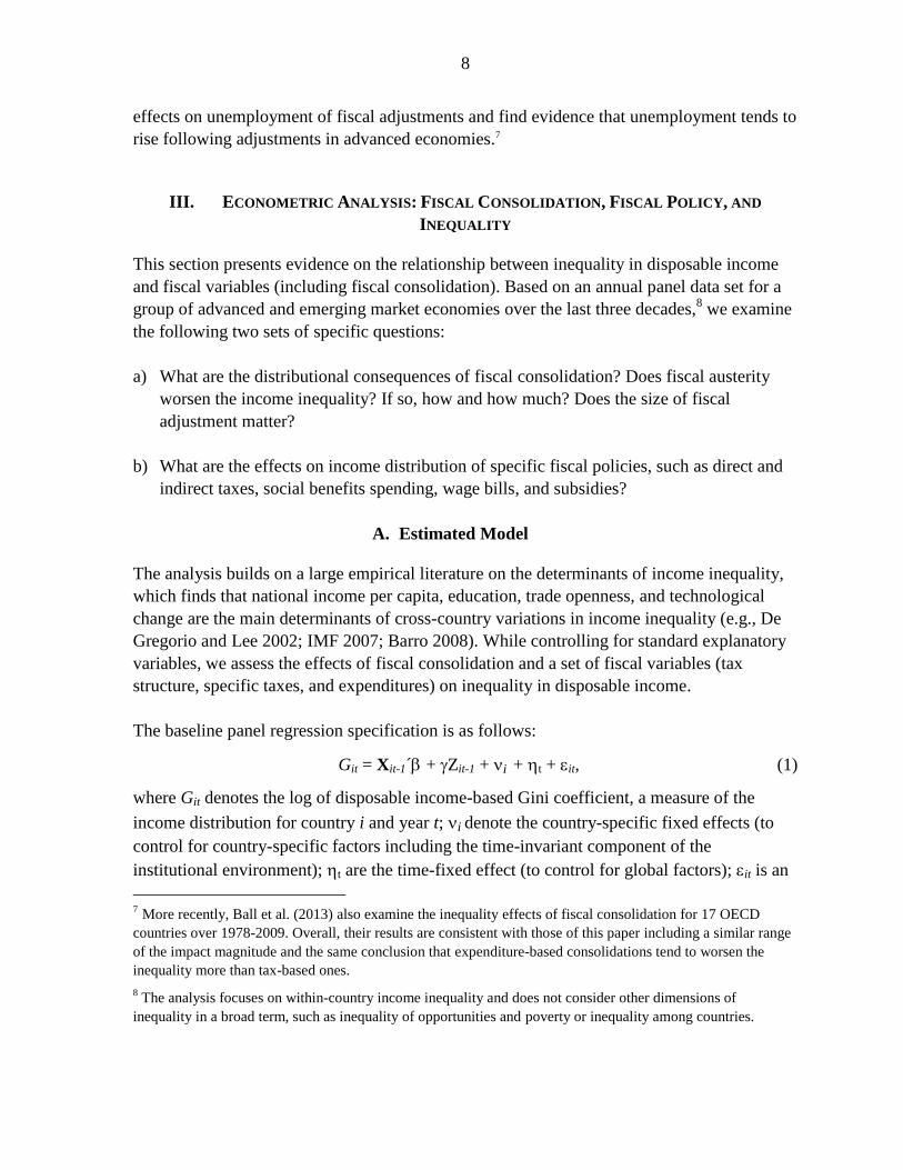
III. ECONOMETRIC ANALYSIS: FISCAL CONSOLIDATION, FISCAL POLICY, AND

INEQUALITY

This section presents evidence on the relationship between inequality in disposable income

and fiscal variables (including fiscal consolidation). Based on an annual panel data set for a

group of advanced and emerging market economies over the last three decades,8 we examine

the following two sets of specific questions:

a) What are the distributional consequences of fiscal consolidation? Does fiscal austerity

worsen the income inequality? If so, how and how much? Does the size of fiscal

adjustment matter?

b) What are the effects on income distribution of specific fiscal policies, such as direct and

indirect taxes, social benefits spending, wage bills, and subsidies?

A. Estimated Model

The analysis builds on a large empirical literature on the determinants of income inequality,

which finds that national income per capita, education, trade openness, and technological

change are the main determinants of cross-country variations in income inequality (e.g., De

Gregorio and Lee 2002; IMF 2007; Barro 2008). While controlling for standard explanatory

variables, we assess the effects of fiscal consolidation and a set of fiscal variables (tax

structure, specific taxes, and expenditures) on inequality in disposable income.

The baseline panel regression specification is as follows:

Git = Xit-1´ + Zit-1 + i + t + it, (1)

where Git denotes the log of disposable income-based Gini coefficient, a measure of the

income distribution for country i and year t; i denote the country-specific fixed effects (to

control for country-specific factors including the time-invariant component of the

institutional environment); t are the time-fixed effect (to control for global factors); it is an

7 More recently, Ball et al. (2013) also examine the inequality effects of fiscal consolidation for 17 OECD

countries over 1978-2009. Overall, their results are consistent with those of this paper including a similar range

of the impact magnitude and the same conclusion that expenditure-based consolidations tend to worsen the

inequality more than tax-based ones.

8 The analysis focuses on within-country income inequality and does not consider other dimensions of

inequality in a broad term, such as inequality of opportunities and poverty or inequality among countries.

9

error term; Xit-1 is a vector of economic control variables; and Zit is the measure of fiscal

consolidation or fiscal variables.

Two econometric methods are employed to estimate the panel regression. The first approach

utilizes the fixed-effects (FE) panel regression, with Driscoll-Kraay standard errors that

robust to very general forms of cross-sectional and temporal dependence. The error structure

is assumed to be heteroskedastic, autocorrelated up to two lags (to account for the persistence

of income inequality), and correlated between the panels (i.e., countries) possibly due to

common shocks, say, to technology or international trade. The second approach adopts a

seemingly unrelated regression (SUR) for panel data which consists of two regression

equations – one for disposable income Gini coefficient and the other for market income Gini

coefficient. If the errors are correlated across the equations (i.e., the unobserved determinants

of inequality in market income and disposable income could be correlated), the SUR

estimator will be more efficient.9 In addition, we use alternative regression specification and

estimation methods as robustness checks, including a dynamic panel regression (see section

C below), as well as ordinary least squares (OLS) and panel-corrected standard error (PCSE)

estimates, which also allow the variance-covariance matrix of the estimates to be consistent

when the error terms are heteroskedastic and/or contemporaneously correlated across panels

or auto-correlated within panel (Beck and Katz, 1995). The results are broadly similar.10

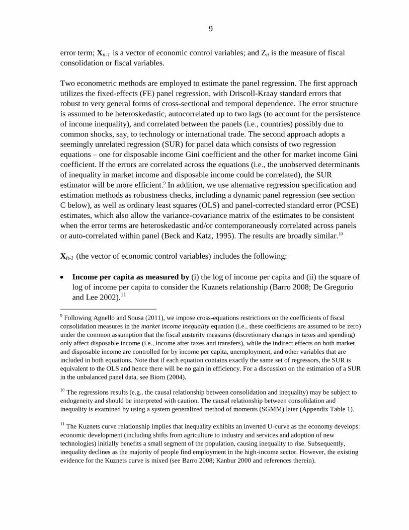
Xit-1 (the vector of economic control variables) includes the following:

Income per capita as measured by (i) the log of income per capita and (ii) the square of

log of income per capita to consider the Kuznets relationship (Barro 2008; De Gregorio

and Lee 2002).11

9 Following Agnello and Sousa (2011), we impose cross-equations restrictions on the coefficients of fiscal

consolidation measures in the market income inequality equation (i.e., these coefficients are assumed to be zero)

under the common assumption that the fiscal austerity measures (discretionary changes in taxes and spending)

only affect disposable income (i.e., income after taxes and transfers), while the indirect effects on both market

and disposable income are controlled for by income per capita, unemployment, and other variables that are

included in both equations. Note that if each equation contains exactly the same set of regressors, the SUR is

equivalent to the OLS and hence there will be no gain in efficiency. For a discussion on the estimation of a SUR

in the unbalanced panel data, see Biorn (2004).

10 The regressions results (e.g., the causal relationship between consolidation and inequality) may be subject to

endogeneity and should be interpreted with caution. The causal relationship between consolidation and

inequality is examined by using a system generalized method of moments (SGMM) later (Appendix Table 1).

11

The Kuznets curve relationship implies that inequality exhibits an inverted U-curve as the economy develops:

economic development (including shifts from agriculture to industry and services and adoption of new

technologies) initially benefits a small segment of the population, causing inequality to rise. Subsequently,

inequality declines as the majority of people find employment in the high-income sector. However, the existing

evidence for the Kuznets curve is mixed (see Barro 2008; Kanbur 2000 and references therein).

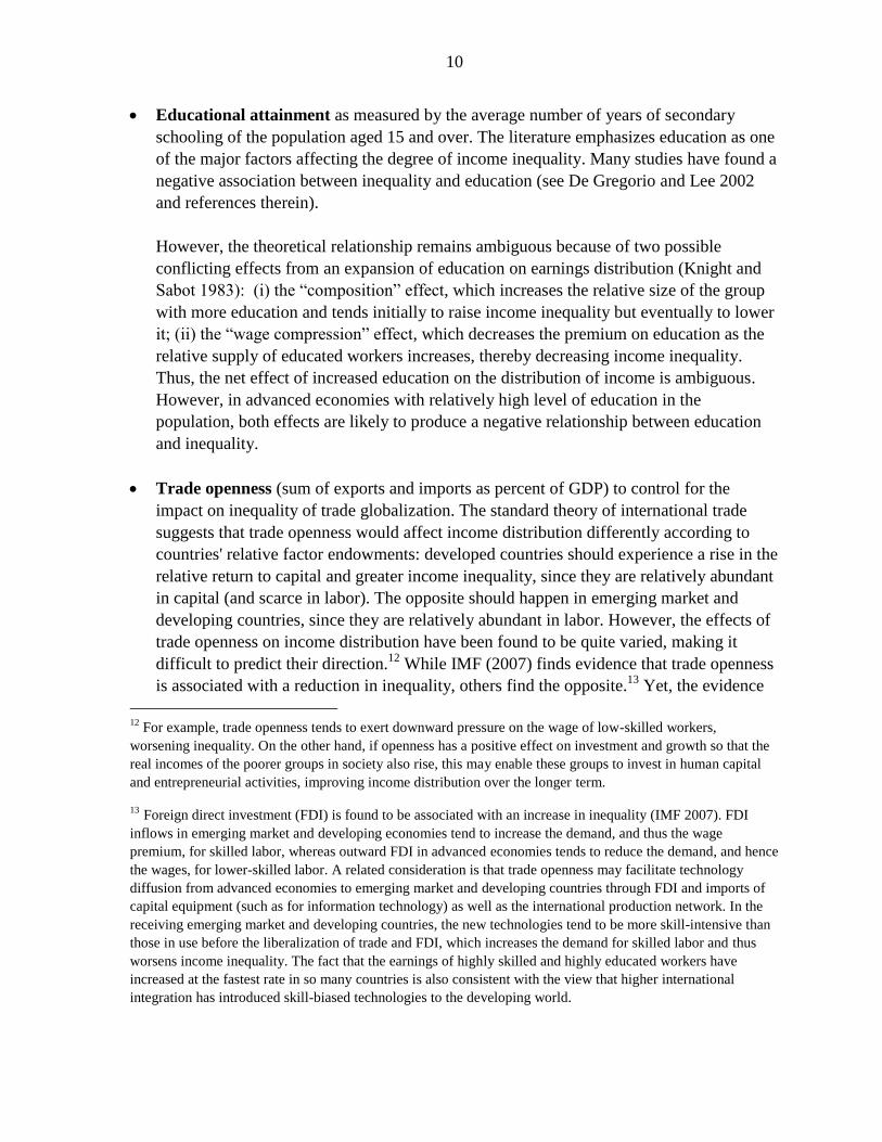
10

Educational attainment as measured by the average number of years of secondary

schooling of the population aged 15 and over. The literature emphasizes education as one

of the major factors affecting the degree of income inequality. Many studies have found a

negative association between inequality and education (see De Gregorio and Lee 2002

and references therein).

However, the theoretical relationship remains ambiguous because of two possible

conflicting effects from an expansion of education on earnings distribution (Knight and

Sabot 1983): (i) the “composition” effect, which increases the relative size of the group

with more education and tends initially to raise income inequality but eventually to lower

it; (ii) the “wage compression” effect, which decreases the premium on education as the

relative supply of educated workers increases, thereby decreasing income inequality.

Thus, the net effect of increased education on the distribution of income is ambiguous.

However, in advanced economies with relatively high level of education in the

population, both effects are likely to produce a negative relationship between education

and inequality.

Trade openness (sum of exports and imports as percent of GDP) to control for the

impact on inequality of trade globalization. The standard theory of international trade

suggests that trade openness would affect income distribution differently according to

countries' relative factor endowments: developed countries should experience a rise in the

relative return to capital and greater income inequality, since they are relatively abundant

in capital (and scarce in labor). The opposite should happen in emerging market and

developing countries, since they are relatively abundant in labor. However, the effects of

trade openness on income distribution have been found to be quite varied, making it

difficult to predict their direction.12

While IMF (2007) finds evidence that trade openness

is associated with a reduction in inequality, others find the opposite.13

Yet, the evidence

12

For example, trade openness tends to exert downward pressure on the wage of low-skilled workers,

worsening inequality. On the other hand, if openness has a positive effect on investment and growth so that the

real incomes of the poorer groups in society also rise, this may enable these groups to invest in human capital

and entrepreneurial activities, improving income distribution over the longer term. 13 Foreign direct investment (FDI) is found to be associated with an increase in inequality (IMF 2007). FDI

inflows in emerging market and developing economies tend to increase the demand, and thus the wage

premium, for skilled labor, whereas outward FDI in advanced economies tends to reduce the demand, and hence

the wages, for lower-skilled labor. A related consideration is that trade openness may facilitate technology

diffusion from advanced economies to emerging market and developing countries through FDI and imports of

capital equipment (such as for information technology) as well as the international production network. In the

receiving emerging market and developing countries, the new technologies tend to be more skill-intensive than

those in use before the liberalization of trade and FDI, which increases the demand for skilled labor and thus

worsens income inequality. The fact that the earnings of highly skilled and highly educated workers have

increased at the fastest rate in so many countries is also consistent with the view that higher international

integration has introduced skill-biased technologies to the developing world.

11

is not conclusive (see Krugman 2007; Meschi and Vivarelli 2007; ADB 2007 for more

discussions).

Unemployment rate: not surprisingly, a greater portion of unemployed (and inactive)

workers are found to be in the bottom income quintile in the OECD countries (Martinez

et al. 2001). Thus, higher unemployment may be associated with greater inequality.

The share of information technology (IT) capital in the total capital stock as a proxy

for skill-biased technological progress (data from Jorgenson and Vu 2007, with a 2011

update). Skill-biased technological progress is found to have made the biggest

contribution to rising income inequality over the recent decades (Autor et al. 1998;

Acemoglu 2003; IMF 2007).

Inflation: inflation tends to hurt the poor more than other income groups and to worsen

inequality (Easterly and Fisher 2001; Bulir 1998). This may be in part due to differences

in wealth composition and transaction patterns (the fraction of household wealth held in

liquid assets, such as currency, decreases with income and wealth) and differential

protection of earnings streams against inflation (wage earners at the bottom of the income

scale are generally much less protected from cyclical real wage fluctuations, such as the

minimum wage).

Incidence of banking crises: banking crises can affect inequality because the poor have

few resources to protect themselves against adverse shocks and very limited access to

credit and insurance. Also, lack of education and skills makes the poor less mobile across

regions and economic sectors, reducing their ability to switch jobs and relocate in

response to shifting demand conditions. However, the evidence is mixed. For example, in

the aftermath of the 1997 Asian crisis, Korea and (to a much lesser degree) the

Philippines saw worsening income distribution, whereas Thailand, Malaysia, and

Indonesia did not. In a recent study, Atkinson and Morelli (2011) do not find any

systematic relationship between macroeconomic disasters and the inequality outcome

(see also Glaeser 2010). We tried the indicator of banking crises, but the results were not

significant and did not alter the main conclusions.

Zit-1 contains measures of fiscal consolidation or fiscal variables as follows:

Fiscal consolidation (spending and tax measures, in percent of GDP) from the action-

based fiscal consolidation data for 17 member countries of the Organization for

12

Economic Cooperation and Development (OECD) for the period of 1978-2009 (from

Devries et al. 2011).14

Ratio of direct to indirect taxes, a measure of the tax structure (from the database of the

Fiscal Affairs Department of the IMF), with a higher value indicating a potentially

greater progressivity of the tax system in a country.

Cyclically adjusted individual and corporate income tax revenue, and cyclically

adjusted indirect tax revenue (all in percent of potential GDP), to account for different

country-specific and tax-specific elasticities.15

Wage bills, social benefits, subsidies, and capital spending (all in percent of potential

GDP) from the database of the Fiscal Affairs Department of the IMF.

B. How Do Different Fiscal Consolidation Measures Affect Income Inequality?

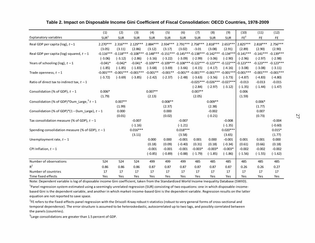
In this section, we focus on the impact on inequality of fiscal consolidation for 17 OECD

countries for 1978-2009 using a parsimonious specification of eq. (1).16 The regression

results from both the SUR and FE approaches suggest that income inequality tends to rise

during periods of fiscal adjustment, especially when the adjustment is based on a

retrenchment in spending.17 A consolidation amounting to 1 percentage point of GDP is

associated with an increase of about 0.6-0.7 percent in inequality of disposable income (as

measured by the Gini coefficient) in the following year (Table 2, columns 1, 4, 7, and 10).18

An alternative dynamic panel regression specification confirms that income inequality

increases following the consolidation, with the cumulative effect peaking after five to six

years and fading by the tenth year (see Section C below). The order of the impact magnitude

14 Alternative sources were also used, including data on consolidations from Alesina and Ardagna (2010) for 17

OECD countries, and structural balance data from the IMF. For interesting discussions on the issues of

identification of fiscal consolidation episodes, measurement of the size of consolidation, and estimation of

short-term growth effects of consolidations, see Perotti (2011) and Alesina and Ardagna (2012) as well as IMF

(2010b). 15

The cyclically-adjusted components were calculated from actual tax revenues adjusted according to the ratio

of potential output to actual output and the tax-specific elasticities for each OECD country. For non-OECD

countries, the new EU member average elasticities from Girouard and Andre (2005) were used.

16 The sample country and period is dictated by the availability of data from Devries et al. (2011).

17 This is with respect to a baseline in which fiscal adjustment is not implemented and deficits continue to be

financed without major disruptions. If the absence of fiscal adjustment leads to a fiscal crisis, with disruptive

consequences for economic activity, income inequality could deteriorate even more.

18

To put this in perspective, note that the average Gini coefficient for disposable income in the 17 OECD

countries increased by about 2 percent between 1995 and 2005.

13

also turns out to be in a similar range – a consolidation of 1 percentage point of GDP is

associated with an increase in the disposable income Gini coefficient by around 0.4 percent

in the following year. The effect of large consolidations (greater than about 1.5 percent of

GDP) is somewhat larger and statistically more significant, compared to small consolidations

(Table 2, columns 2, 5, 8, and 11).19

Comparing spending-based consolidations with tax-based ones, the coefficients of measures

of spending-based consolidations are statistically significant and of positive sign (+),

indicating that spending cuts are associated with an increase in inequality. The estimated

coefficients suggest that a spending cut of 1 percentage point of GDP is associated with an

increase of about 1.5–2 percent in the Gini coefficient (columns 3, 6, 9, and 12). In contrast,

the coefficients of tax-based consolidations are not significant but of negative sign (–). The

contrasting results between spending- and tax-based consolidations are intuitive – for

example, income tax measures can actually lower the inequality, depending on the

progressivity of the particular measure, while the indirect effects through an increase in

unemployment due to their recessionary effects may increase inequality. Taken together,

therefore, the net effects of tax-based consolidations can be somewhat ambiguous.

On the other hand, the progressivity of taxation, as measured by the ratio of direct to indirect

taxes, is negatively associated with disposable income inequality (Figure 3). Columns (7)-(9)

suggest that an increase of 1 in that ratio is associated with a reduction of about 2.5 percent in

inequality.20 To put this in perspective, let us consider an illustrative example. In 2009, the

disposable income-based Gini coefficients in Denmark and Portugal were 26.5 and 34, while

the ratios of direct to indirect taxes were 1.91 and 0.74, respectively. The difference in the

direct to indirect tax ratio between the two countries explains about 12 percent of the

difference in inequality between them.

Consistent with the literature, education and trade openness are significantly associated with

lower inequality. According to the estimated coefficients, a 1 percent increase in the average

years of schooling is associated with about 0.04-0.12 percent reduction in inequality. On the

other hand, a 1 percentage point of GDP increase in trade openness is associated with about

0.1 percent reduction in inequality. Evidence of an inverse U-shaped relationship between

income per capita and inequality is also found, with the inequality starting to decrease when

real income per capita exceeds about $17,700 in 2005 international dollars (based on

19

This seems to reflect the fact that large consolidations tend to be longer in duration and mostly spending-

based. Spending-based fiscal adjustment has been found to have more pronounced effects on inequality than

tax-based adjustment. This is confirmed in the case study presented later in this paper.

20 However, the FE coefficient estimates (columns 10-12) turn out to be smaller in size and insignificant.

14

column 1).21 Also, it is interesting to note that the coefficients of unemployment are of

positive sign but insignificant, after controlling for measures of consolidation (columns 4-12)

– for example, if we drop the fiscal consolidation variable from the regression in column (4),

then the coefficient of unemployment becomes significant at 1 percent (the coefficient

estimate is 0.003 and its implied magnitude of impact on inequality turns out to be similar to

those reported in Section D below).

C. Dynamic Effects of Fiscal Consolidation on Income Inequality

Since fiscal consolidations may have lingering effects on inequality over time, we further

investigate the dynamic impact of fiscal consolidation on inequality by adopting a dynamic

panel regression specification, again for the 17 OECD countries over 1978-2009. To this end,

a univariate autoregressive model is extended to include the current and lagged impacts of

the fiscal shock and to derive the relative impulse response functions (IRFs) in an unbalanced

annual panel:22

, (2)

where i is a country; t is a year; git denotes the Gini coefficient for disposable income; vi are

country-specific fixed effects; t are time-fixed effects (to control for global factors); and Fit

is a measure of fiscal consolidation (as percent of GDP) from Devries, et al. (2011). The

number of lags has been restricted to two; the presence of additional lags was rejected by the

data.23

Impulse response functions (IRFs) are obtained by simulating a shock on the fiscal

consolidation. The shape of these response functions depends on the value of the and

coefficients. For instance, the simultaneous response will be 0, while the one-year ahead

response will be 1 + 0 0, and so on.

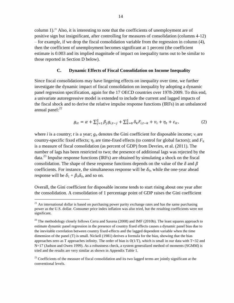
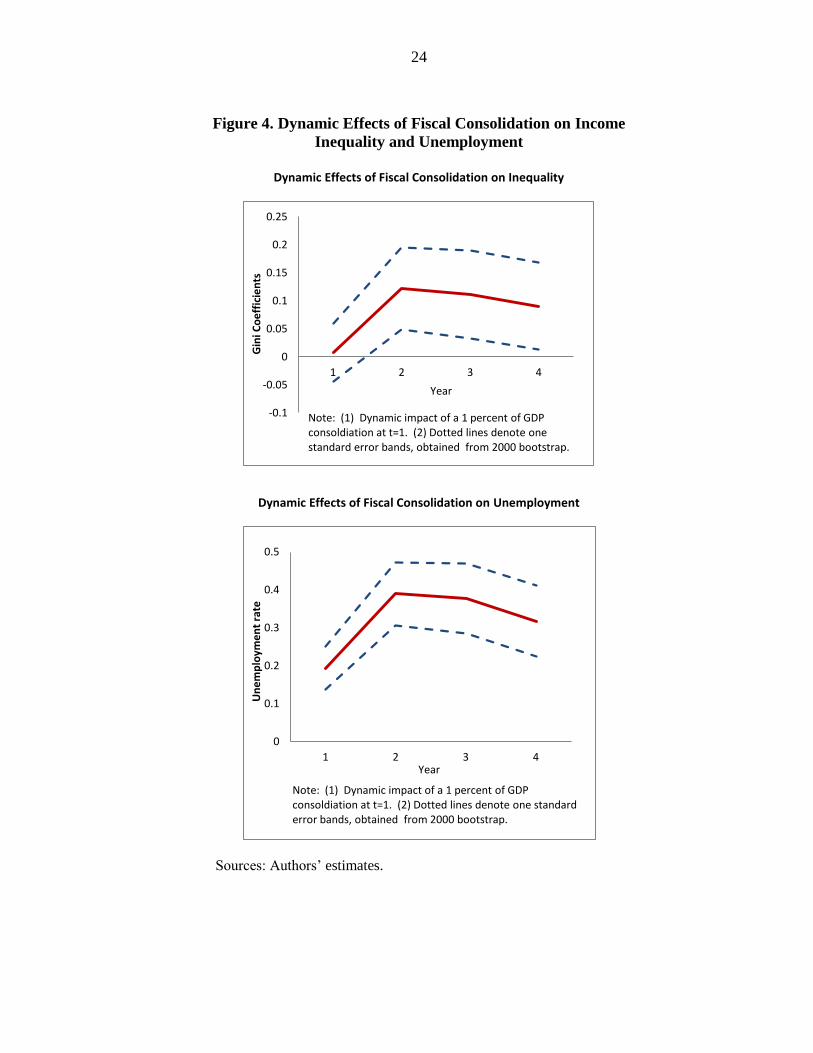
Overall, the Gini coefficient for disposable income tends to start rising about one year after

the consolidation. A consolidation of 1 percentage point of GDP raises the Gini coefficient

21 An international dollar is based on purchasing power parity exchange rates and has the same purchasing

power as the U.S. dollar. Consumer price index inflation was also tried, but the resulting coefficients were not

significant. 22

The methodology closely follows Cerra and Saxena (2008) and IMF (2010b). The least squares approach to

estimate dynamic panel regression in the presence of country fixed effects causes a dynamic panel bias due to

the inevitable correlation between country fixed-effects and the lagged dependent variable when the time

dimension of the panel (T) is small. Nickell (1981) derives a formula for the bias, showing that the bias

approaches zero as T approaches infinity. The order of bias is O(1/T), which is small in our data with T=32 and

N=17 (Judson and Owen 1999). As a robustness check, a system generalized method of moments (SGMM) is

tried and the results are very similar as shown in Appendix Table 1.

23 Coefficients of the measure of fiscal consolidation and its two lagged terms are jointly significant at the

conventional levels.

15

by 0.13 points in the second year, and by 0.4 cumulatively over five years (Figure 4).24

On

average, the 0.13 and 0.4 increases in the Gini are equivalent to increases in inequality of

0.4 percent and 1.3 percent, respectively (the OECD average of the Gini coefficient for

disposable income in the sample period is 30.02). The order of magnitude of the impact (a

0.4 percent rise in the first two years) is comparable to the 0.6-0.7 percent increase suggested

by the baseline regression (Table 2). Also, an alternative measure of fiscal consolidation

from Alesina and Ardagna (2010) is used.25

The result is qualitatively similar, suggesting that

a consolidation raises the Gini coefficient by 0.12 points in the second year, and by 0.66

cumulatively over five years.

To gauge the impact of consolidation on inequality through the channel of unemployment,

the same model described above is used to derive the dynamic impact of consolidation on

unemployment (Figure 4). Consolidation seems to start affecting unemployment

immediately, with a consolidation of 1 percent of GDP leading to a 0.19 percentage point

increase in the unemployment rate in the first year,26 and 1.5 percentage points cumulatively

over five years. The impact subsequently gets smaller, disappearing by the tenth year and

then turning negative. Coefficients of the measure of fiscal consolidation and its two lagged

terms are jointly significant at the conventional level. However, if an alternative measure of

fiscal consolidation from Alesina and Ardagna (2010) is used for the same exercise on

unemployment, none of the coefficients of the consolidation and its two lagged terms are

individually or jointly significant. According to the lower estimates in Table 3 (columns 1-8),

a 1 percentage point increase in unemployment rate is associated with an increase in

inequality of about 0.3-0.4 percent, which implies that about 15-20 percent of the increase in

inequality due to consolidation may be occurring via the increase in unemployment.

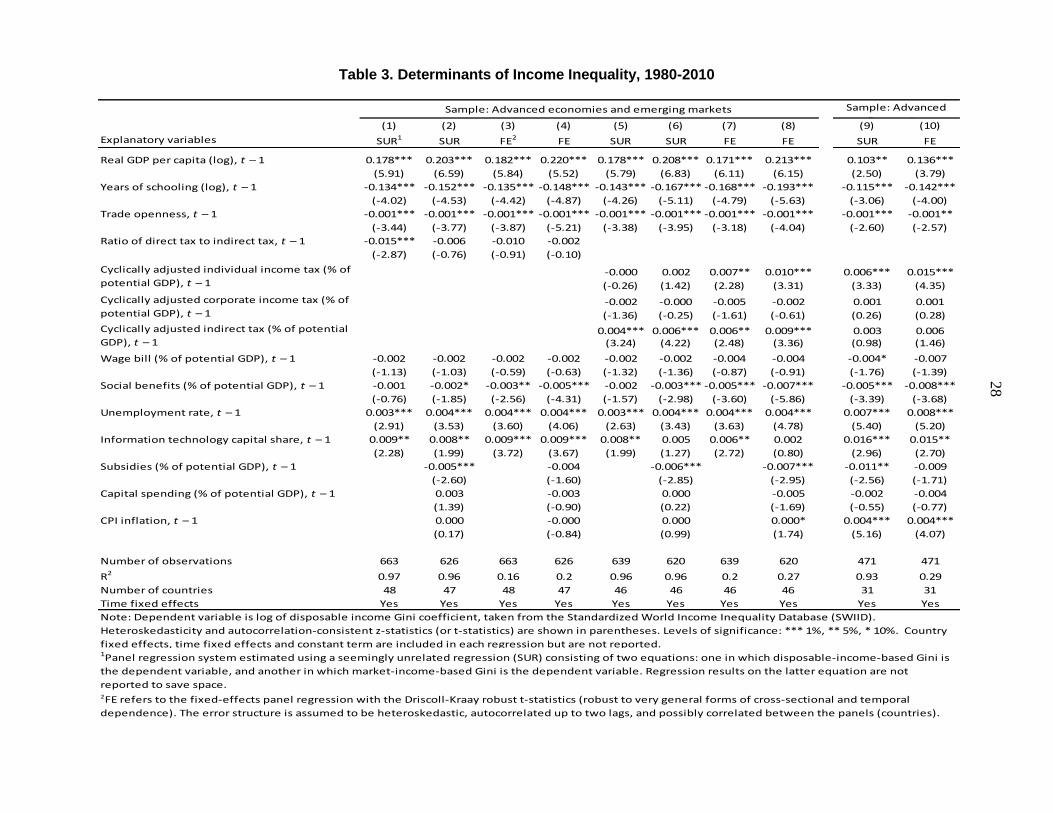
D. Fiscal Policy and Income Inequality

So far we have examined the inequality impact of fiscal consolidation. Now, we turn to a set

of fiscal variables (tax structure, specific taxes and expenditures) and assess their effects on

disposable income inequality in a sample of 48 advanced and emerging market economies

during 1980-2010 by using the regression specification of eq. (1). The regression results

24

Results are closely similar when Gini coefficient or its log is used as the dependent variable in the dynamic

panel regression. The Gini coefficient is employed here to facilitate interpretation of the chart.

25 The measure is a dummy variable taking a value of 1 in the year of a large consolidation and 0 otherwise,

where a large fiscal consolidation is defined by Alesina and Ardagna (2010) to be larger than 1.5 percent of

GDP. Thus, the result using this dummy variable is not directly comparable to that based on the consolidation

measure (in percent of GDP) from Devries et al. (2011).

26 This magnitude is similar to that in Ball et al. (2011).

16

suggest that higher social spending and (to a lesser degree in terms of statistical significance)

greater progressivity in taxation tend to be associated with lower inequality (Table 3). In

particular, the coefficients of the ratio of direct to indirect taxes as a measure of progressivity

of taxation are negatively associated with disposable income inequality in columns (1)-(4).

According to the estimates in column (1), an increase in the ratio by 1 is associated with

about 1.5 percent reduction in inequality as captured by the Gini coefficient for disposable

income. In columns 2-4, however, the coefficients lose statistical significance, as they turn

out to be sensitive to other conditional variables. According to the estimates in column (1),

an increase in the ratio by 1 is associated with about 1.5 percent reduction in inequality as

captured by the Gini coefficient for disposable income.

Major categories of taxes (personal income taxes, corporate income taxes, indirect taxes) are

also considered in the regressions. The coefficients of indirect tax are significant and of the

expected (+) sign, which indicates an association with higher income inequality, in the

sample of 48 advanced and emerging market economies (columns 5-8). A 1 percentage point

of potential GDP increase in indirect taxes is associated with a 0.4-0.9 percent rise in

inequality. However, the coefficients of indirect taxes become insignificant in the OECD

country sample (columns 9-10), although the implied impact magnitude is comparable to that

in the sample of 48 economies. The coefficients of corporate taxes are of the expected sign (–

), which indicates progressivity of the tax, except for columns (9) and (10). However, none of

them are significant at the conventional levels.27

On the expenditure side, social benefits (including health care, social security pensions, and

unemployment compensation) are statistically significantly associated with lower inequality

(except for columns 1 and 5 in which the coefficients are insignificant, albeit negatively

signed). This positive contribution of government social benefits spending to income

distribution may occur through two channels. The first is that part of social expenditure

consists of direct transfers to the poor, increasing their income and redistributing income

from rich to poor. The second is that social expenditure may promote access for the poor to

education and other human-capital-enhancing activities, such health care, thereby

contributing to future income equality. Based on the significant coefficients (columns 2-4

and 6-8), the implied magnitude of the impact suggests that increasing social benefits

spending by 1 percentage point of potential GDP is associated with a 0.2-0.7 percent

reduction in inequality. The order of magnitude of the impact is quite similar to that found in

De Gregorio and Lee (2002).

27

Also, the coefficients of individual income taxes are mostly of positive sign and significant (columns 7-10).

But the collected tax revenue as percent of potential GDP may not necessarily indicate the degree of

progressivity in individual income taxation.

17

The government wage bill, subsidies, and capital spending also tend to be negatively

associated with inequality, although the regression results turn out to be fragile. The negative

coefficients of the wage bill suggest that increases in government employee pay are

associated with lower inequality, which seems to imply that government employees occupy a

below-average position in the income distribution of the population. Interestingly, the

opposite sign is obtained for the coefficient of wage bills in low income countries (higher

government wages widen inequality), which suggests that government employees may be

better compensated than the average employee in those countries (not reported).

Subsidies – including transfers to public corporations to compensate for operating losses on

public transportation, electricity, and other services – tend to be associated with lower

inequality.28 While the statistical significance of subsidies is sensitive to estimation methods,

the seemingly unrelated regression estimates suggest that an increase in subsidies of

1 percentage point of potential GDP is associated with a 0.5-1.1 percent reduction in

inequality. Of course, a policy to reduce inequality that targets these subsidies to low-income

consumers could be even more effective and less costly.

Unemployment is found to be a significant determinant of income inequality. A 1 percentage

point increase in the unemployment rate is associated with a 0.3-0.4 percent increase in

inequality (and 0.7-0.8 percent for advanced economies). In addition, it is noteworthy that the

coefficients of basic explanatory variables (including income per capita, average years of

schooling, and trade openness) are of the expected sign and mostly significant at 1-10 percent

levels.29 In particular, it is interesting to find that the impact of education on inequality tends

to be a bit greater in the broad sample than in the advanced economy group: an increase in

the number of years of schooling of 1 percent is associated with a 0.13-0.19 percent

reduction in inequality. Also, the coefficients of a measure of skill-biased technological

progress are all of the expected sign (+) and significant except for columns 6 and 8. If we use

the significant coefficients to get a sense of the order of magnitude, the results suggest that a

1 percentage point in the IT share of total capital is associated with a 1.5-1.6 percent increase

in inequality for the sample of advanced economies (columns 9-10). To put this in

perspective, let us take the cases of Korea and the United States. In 2007, the IT capital share

was 3.5 in Korea and 8.2 percent in the United States, and in 2008 the respective Gini

coefficients for disposable income were 31.4 and 36. Other things being equal, the difference

28

However, universal price subsidy programs (e.g., fuel subsidy) are often found to be a very expensive and

inefficient tool for redistribution, especially in low income countries. For the sake of efficiency and

effectiveness, expenditure reforms should focus on reducing universal price subsidies, improving the capacity to

implement better targeted transfers, and gradually expanding social insurance systems (see Coady et al., 2010). 29

The square term of log of income per capita is not included, as it often becomes insignificant or changes its

sign in the regressions in which an array of fiscal variables are controlled for in the sample of 48 advanced and

emerging economies (not reported to save space).

18

in the IT capital share can account for more than 48 percent of the gap of 4.6 Gini points

between the two countries. On the other hand, inflation turns out to be significant mainly in

the advanced economy sample, while mostly insignificant in the sample of 48 advanced and

emerging economies.

Finally, the results are broadly similar if we use either alternative data sets (from World

Income Inequality Data (WIID), Luxembourg Income Study (LIS) and the World Bank’s

PovcalNet) or alternative measures of inequality (including ratios of top to bottom

quintiles/deciles) (Appendix Table 2).

IV. CASE STUDY OF FISCAL CONSOLIDATION EPISODES

We examine twelve selected large fiscal consolidation episodes (six spending-based and six

tax-based) and highlight their salient features. To do this, we first classified all the

consolidation episodes from Devries et al. (2011) into three categories according to the

magnitude of inequality changes after the consolidation (bottom 1/3 percentile, middle 1/3

percentile, and top 1/3 percentile), and then picked two largest spending-based and two

largest tax-based episodes (as measured by the size of consolidation) from each category.

The six spending-based consolidation episodes are Austria, 1996-97; Germany, 1992-99;

Iceland, 1993-99; Norway, 1993-97; Spain, 1992-98; and Sweden, 1994-2001. The six tax

based consolidation episodes are Australia, 1994-96; Belgium, 1996-98; France, 1994-97;

Iceland, 2004-06; the Netherlands, 2004-05; and the United Kingdom, 1994-98.30

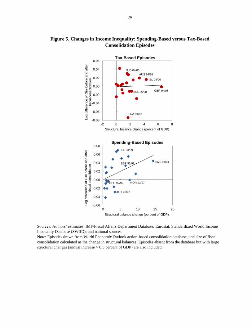
Overall, the impact on income distribution seems to vary with the composition of the

consolidation package, a country’s position in the business cycle, and labor market

conditions. Nonetheless, some patterns emerge from these episodes. We find that spending-

based consolidations tend to be associated with increases in income inequality (Figure 5).

Looking at the simple average, inequality increased about 2 percent after the spending-based

consolidations, while it rose about 1 percent in the case of the tax-based episodes. This seems

to be largely because lower income earners are typically more affected by spending cuts as a

larger portion of their disposable income comes from public spending and they are more

vulnerable to losing their jobs. In contrast, tax-based consolidations tend to have mixed net

effects on inequality: direct taxes tend to be progressive, whereas indirect taxes are

regressive. Looking at historical episodes, spending-based consolidations (as in Iceland,

1993-99, and Sweden, 1994-2001), or tax-based consolidations with a significant portion of

expenditure measures (as in the United Kingdom, 1994-98) tend to be larger in size and

30

Many of these episodes took place as European Union member states attempted to meet the Maastricht

criteria (i.e., the convergence criteria) for adoption of the euro as their currency.

19

longer in duration, which could be another reason for the more pronounced effects on

inequality, than tax-based consolidations.31

That said, the net effect of a fiscal consolidation on inequality depends crucially on the

specific composition of austerity measures. Cuts in social benefits tend to worsen inequality

more than other spending reductions, for example, public wage cuts. Fiscal consolidations in

Spain, 1992-98, and Norway, 1993-97, consisted of across-the-board spending cuts, while

protecting social benefits. Tax-based consolidations that rely more on indirect taxes or are

mixed with expenditure cuts tend to worsen inequality (e.g., Iceland, 2004-06). Also,

addressing tax evasion and tax loopholes was an alternative way to generate public savings

without necessarily elevating the income inequality (e.g., Germany 1992-99).

Unemployment could be an important factor behind the increases in inequality, but it is

difficult to disentangle the effect of unemployment from that of other factors without using

econometric analysis. Looking at the simple average unemployment rate (i.e., without

controlling for any other factors), unemployment increased by 0.26 percentage points in the

first year of the consolidation, which is comparable to the 0.19 percentage points that we find

from the econometric analysis (Sub-section C of Section II).32 In terms of the timing of

consolidation, consolidations undertaken during recessions could have a greater impact on

inequality. In particular, social benefit cuts and tax increases amid rising unemployment (as,

for example, in Spain, 1992-98, and Sweden, 1994-2001) seem to have led to higher

inequality than those undertaken during non-recession periods (such as those in Austria,

1996-97, and Belgium, 1996-98). This suggests the importance of unemployment benefits

and more generally, social protection in assisting the most vulnerable. In a similar vein, to the

extent that active labor market measures (such as job search assistance, training, and

incentives to hire workers) help alleviate (long-term) unemployment, they may help mitigate

the deterioration in income distribution.

The recent consolidation experience in Ireland shares many of these features, although it is

difficult to disentangle the distributional impact of consolidation itself from that of the

financial crisis and ensuing recession. Inequality initially fell as upper income groups

suffered major income losses while taxes increased and redistributive social transfers

expanded. However, the impact of the deepening crisis and recession quickly spilled over to

31

On average, the duration and size of the six spending-based consolidations were about 6 years and 5 percent

of GDP (as measured by change in structural balance), compared to about 3 years and 4 percent of GDP in the

case of the six tax-based consolidations.

32 Yet there is some difference between spending- and tax-based consolidations. In the spending-based cases,

the unemployment rate was, on average, higher by 0.67 percentage points in the first year of the consolidation,

compared to that a year before. By contrast, the average unemployment rate was lower by 0.15percentage points

in the first year of the tax-based consolidations.

20

broader income groups via rising unemployment. Against this backdrop, the government had

to embark on a large fiscal consolidation in 2010 due to adverse market reactions to the

soaring sovereign debt. The consolidation package was sizable and mainly expenditure-

based. Public sector wage cuts mainly affected the middle upper class which might have

mitigated the rising inequality, whereas social benefit cuts (family allowances, old-age

benefits) heavily weighed on the lower income group, contributing to higher inequality (see

2010 Survey on Income and Living Conditions for Ireland). Despite some offsetting tax

measures that were progressive in nature, the largely spending-based consolidation in 2010

amid deepening crisis and recession appears to start worsening inequality.

V. CONCLUDING REMARKS

This paper examined the effects of fiscal consolidation and a set of fiscal variables (tax

structure, specific taxes, and expenditures) on inequality in disposable income by using an

econometric analysis for a panel of advanced and emerging economies for the last three

decades as well as a case study of selected consolidation episodes. The results suggest that

fiscal consolidations tend to increase income inequality. On average, a consolidation of 1

percentage point of GDP is associated with an increase in the disposable income Gini

coefficient of around 0.4-0.7 percent over the first two years. Spending-based consolidations

tend to significantly worsen inequality, relative to tax-based consolidations. So do large-sized

consolidations. The paper also found that unemployment is an important channel through

which consolidation increases inequality.

The composition of austerity measures also matters, and better-designed tax and social

benefits policies can help mitigate the adverse effects on income inequality of fiscal

adjustments. Indeed, progressive taxation and social benefits are consistently associated with

lower inequality for disposable income. These results are consistent with the view that in

advanced economies, reforms since the 1980s have been a factor behind rising income

inequality by lessening the generosity of social benefits and the progressivity of income tax

systems.

More generally, fiscal policy can favorably influence long-term trends in both inequality and

growth by promoting education and training among low- and middle-income workers.

Education and skill-biased technological progress are associated with lower and greater

inequality, respectively. In addition, trade openness tends to be associated with lower

inequality. Evidence of the Kuznets inverted U-shaped relationship between income per

capita and inequality is also found in the data.

Going forward, large fiscal adjustments are expected to be required in many countries for a

long time in order to reduce debt-to-GDP ratios to sustainable levels. For reasons of equity

and also of political economy, fiscal adjustments that are viewed as being unfair are unlikely

to be sustainable. It is therefore critical that the costs associated with fiscal consolidations

and weaker growth be shared equitably throughout the economy.

21

Figure 1. Selected European Economies: Change in Unemployment and the Gini

Coefficient, 2007-10

Unemployment and the Gini Coefficient, 2007-10

Sources: Authors’ estimates; European Union, Statistics on Income

and Living Conditions (EU-SILC).

BEL

BGR

CZE

DNK

DEU

IRL

GRC

ESP

FRA

ITA CYP

LTU

LUX

HUN

MLT

NLD

AUT

POL

PRT

SVN

SVK

FIN

SWE GBR

NOR

-5

-4

-3

-2

-1

0

1

2

3

4

5

-5 0 5 10 15

Absolu

te c

hange in

Gin

i coeff

icie

nt

Change in unemployment (percentage points)

22

Figure 2. Trends in Disposable Income Inequality: Gini Coefficient, 1985-2010

(Scale, 0-100)

Sources: Authors’ estimates based on the Standardized World

Income Inequality Database (SWIID)

Note: A higher number indicates greater inequality.

AUS

AUT BEL

CAN

DNK

FIN

FRA

DEU

GRC

IRL

ISR

ITA

JPN

LUX

NLD

NZL

NOR

PRT

ESP

SWE

GBR USA

20

25

30

35

40

20 25 30 35 40

2000

–10

1985–95

Advanced

AZE

BGR

HUN

POL

ROU

UKR

CIV

GHA

KEN

MDG

MWI

NGA

SEN

ZAF

TZA

ZMB

EGY

JOR

PAK

ARG

BOL

BRA

CHL

COL

MEX

PER

CHN

IND

IDN MYS

PHL

15

25

35

45

55

65

15 25 35 45 55 65

2000

–10

1985–95

Emerging and Low Income

23

Figure 3. Ratio of Direct to Indirect Taxes and Social Benefits Spending, 1980-2009

Sources: Authors’ estimates; IMF/Fiscal Affairs Department database; Standardized World Income Inequality

Database (SWIID); and national sources.

0

1

2

3

4

5

1980 1985 1990 1995 2000 2005 2009

Advanced Emerging Low Income

0

4

8

12

16

20

1990 1995 2000 2005 2009

Ratio of Direct to Indirect Taxes and Inequality

Social Benefits and Subsidies and Inequality

Gin

i (dis

posa

ble

inco

me)

Gin

i (dis

posa

ble

inco

me)

Ratio of Direct to Indirect TaxesSocial Benefits and Subsidies

(percent of potential GDP)

Ratio of direct to indirect taxesSocial benefits and subsidies (percent of potential GDP)

24

Figure 4. Dynamic Effects of Fiscal Consolidation on Income

Inequality and Unemployment

Dynamic Effects of Fiscal Consolidation on Inequality

Dynamic Effects of Fiscal Consolidation on Unemployment

Sources: Authors’ estimates.

-0.1

-0.05

0

0.05

0.1

0.15

0.2

0.25

1 2 3 4

Gin

i Co

eff

icie

nts

Note: (1) Dynamic impact of a 1 percent of GDP consoldiation at t=1. (2) Dotted lines denote one standard error bands, obtained from 2000 bootstrap.

Year

0

0.1

0.2

0.3

0.4

0.5

1 2 3 4

Un

em

plo

yme

nt

rate

Note: (1) Dynamic impact of a 1 percent of GDP consoldiation at t=1. (2) Dotted lines denote one standard error bands, obtained from 2000 bootstrap.

Year

25

Figure 5. Changes in Income Inequality: Spending-Based versus Tax-Based

Consolidation Episodes

Sources: Authors’ estimates; IMF/Fiscal Affairs Department Database; Eurostat; Standardized World Income

Inequality Database (SWIID); and national sources.

Note: Episodes drawn from World Economic Outlook action-based consolidation database, and size of fiscal

consolidation calculated as the change in structural balances. Episodes absent from the database but with large

structural changes (annual increase > 0.5 percent of GDP) are also included.

AUS 94/96

FRA 94/97

GBR 94/98 BEL 96/98

ISL 04/06

NLD 04/05

-0.08

-0.06

-0.04

-0.02

0.00

0.02

0.04

0.06

-2 0 2 4 6 8

Log d

iffe

rence o

f G

ini befo

re a

nd a

fter

fiscal c

onsolid

atio

n

Structural balance change (percent of GDP)

Tax-Based Episodes

AUT 96/97

DEU 92/99

ESP 92/98

NOR 93/97

SWE 94/01

ISL 93/99

-0.06

-0.04

-0.02

0.00

0.02

0.04

0.06

0.08

0 5 10 15 20

Log d

iffe

rence o

f G

ini befo

re a

nd a

fter

fiscal c

onsolid

atio

n

Structural balance change (percent of GDP)

Spending-Based Episodes

26

Table 1. Pairwise Correlation of Measures of Income Distribution and Unemployment, 1980-2010

Sample: Advanced and Emerging Economies

Gini

(disposable

income)

Gini

(disposable

income),

alternative

Gini

(market

income)

Labor

income

share

top 10%

income

share

top/bottom

quintiles

top/bottom

deciles

Unemploy

ment

Gini (disposable income)1 1

Gini (disposable income), alternative2 0.95 1

Gini (market income)3 0.70 0.40 1

Labor income share4 -0.26 -0.36 0.11 1

top 10% income share5 0.64 0.65 0.33 -0.46 1

top/bottom quintiles6 0.54 0.62 0.47 -0.44 0.60 1

top/bottom deciles7 0.71 0.87 0.37 -0.16 0.30 0.50 1

Unemployment rate80.16 0.19 0.17 -0.06 0.26 0.27 0.17 1

Source: See Appendix 1 for more details.

1/ Disposable income Gini coefficients from Standardized World Income Inequality Database (Solt, 2012)

2/ Disposable income Gini coefficients, compiled by the authors using data from Eurostat, World Income Inequality Database,

PovcalNet, and national sources.

3/ Market income Gini coefficients from Standardized World Income Inequality Database (Solt, 2012)

4/ Labor income share from EU KLEMS Database

5/ Top 10% income share from The World Top Incomes Database

6, 7/ Income quintile/deciles, compiled by the authors using data from Eurostat, World Income Inequality Database, PovcalNet,

and national sources.

8/ Unemployment rate from OECD, and World Development Indicators

2

7

(1) (2) (3) (4) (5) (6) (7) (8) (9) (10) (11) (12)

Explanatory variables SUR1 SUR SUR SUR SUR SUR SUR SUR SUR FE2 FE FE

Real GDP per capita (log), t –1 2.270*** 2.316*** 2.129*** 2.884*** 2.934*** 2.791*** 2.758*** 2.818*** 2.653*** 2.825*** 2.818*** 2.756***

(3.05) (3.11) (2.86) (3.12) (3.17) (3.02) -3.01 (3.08) (2.91) (2.89) (2.90) (2.90)

Real GDP per capita (log) squared, t – 1 -0.116*** -0.118*** -0.108*** -0.148*** -0.151*** -0.145***-0.138*** -0.142*** -0.134*** -0.141*** -0.141*** -0.139***

(-3.06) (-3.12) (-2.86) (-3.16) (-3.22) (-3.09) (-2.99) (-3.06) (-2.90) (-2.96) (-2.97) (-2.98)

Years of schooling (log), t – 1 -0.041* -0.042* -0.041* -0.109*** -0.109*** -0.108***-0.122*** -0.123*** -0.122*** -0.123*** -0.123*** -0.123***

(-1.85) (-1.85) (-1.83) (-3.68) (-3.69) (-3.66) (-4.15) (-4.17) (-4.16) (-3.08) (-3.08) (-3.11)

Trade openness, t – 1 -0.001*** -0.001*** -0.001*** -0.001** -0.001** -0.001** -0.001*** -0.001*** -0.001*** -0.001*** -0.001*** -0.001***

(-3.72) (-3.69) (-3.85) (-2.42) (-2.37) (-2.48) (-3.63) (-3.56) (-3.73) (-4.87) (-4.83) (-4.80)

Ratio of direct tax to indirect tax, t – 1 -0.025*** -0.026*** -0.027*** -0.013 -0.013 -0.015

(-2.84) (-2.97) (-3.12) (-1.35) (-1.44) (-1.47)

Consolidation (% of GDP), t – 1 0.006* 0.007** 0.007** 0.006

(1.79) (2.13) (2.05) (1.59)

Consolidation (% of GDP)*Dum_Large,3 t – 1 0.007** 0.008** 0.009** 0.006*

(1.99) (2.37) (2.38) (1.77)

Consolidation (% of GDP)*(1 – Dum_Large), t – 1 0.000 0.000 -0.002 0.007

(0.01) (0.02) (-0.21) (0.73)

Tax consolidation measure (% of GDP), t – 1 -0.007 -0.007 -0.008 -0.004

(-1.16) (-1.21) (-1.35) (-0.60)

Spending consolidation measure (% of GDP), t – 1 0.016*** 0.018*** 0.020*** 0.015*

(3.11) (3.58) (3.65) (1.77)

Unemployment rate, t – 1 0.000 0.000 -0.001 0.001 0.000 -0.001 0.001 0.001 0.000

(0.18) (0.09) (-0.40) (0.31) (0.18) (-0.34) (0.61) (0.66) (0.18)

CPI Inflation, t – 1 -0.001 -0.001 -0.001 -0.003* -0.003* -0.003* -0.002 -0.002 -0.002

(-0.85) (-0.89) (-0.88) (-1.79) (-1.85) (-1.86) (-1.56) (-1.55) (-1.62)

Number of observations 524 524 524 499 499 499 485 485 485 485 485 485

R2 0.86 0.86 0.86 0.87 0.87 0.87 0.87 0.87 0.87 0.26 0.26 0.27

Number of countries 17 17 17 17 17 17 17 17 17 17 17 17

Time fixed effects Yes Yes Yes Yes Yes Yes Yes Yes Yes Yes Yes Yes

3Large consolidations are greater than 1.5 percent of GDP.

Note: Dependent variable is log of disposable income Gini coefficient, taken from the Standardized World Income Inequality Database (SWIID). 1Panel regression system estimated using a seemingly unrelated regression (SUR) consisting of two equations: one in which disposable-income-

based Gini is the dependent variable, and another in which market-income-based Gini is the dependent variable. Regression results on the latter

equation are not reported to save space.2FE refers to the fixed-effects panel regression with the Driscoll-Kraay robust t-statistics (robust to very general forms of cross-sectional and

temporal dependence). The error structure is assumed to be heteroskedastic, autocorrelated up to two lags, and possibly correlated between

the panels (countries).

Table 2. Impact on Disposable Income Gini Coefficient of Fiscal Consolidation: OECD Countries, 1978-2009

28

(1) (2) (3) (4) (5) (6) (7) (8) (9) (10)

Explanatory variables SUR1 SUR FE2 FE SUR SUR FE FE SUR FE

Real GDP per capita (log), t – 1 0.178*** 0.203*** 0.182*** 0.220*** 0.178*** 0.208*** 0.171*** 0.213*** 0.103** 0.136***

(5.91) (6.59) (5.84) (5.52) (5.79) (6.83) (6.11) (6.15) (2.50) (3.79)

Years of schooling (log), t – 1 -0.134*** -0.152*** -0.135*** -0.148*** -0.143*** -0.167*** -0.168*** -0.193*** -0.115*** -0.142***

(-4.02) (-4.53) (-4.42) (-4.87) (-4.26) (-5.11) (-4.79) (-5.63) (-3.06) (-4.00)

Trade openness, t – 1 -0.001*** -0.001*** -0.001*** -0.001*** -0.001*** -0.001*** -0.001*** -0.001*** -0.001*** -0.001**

(-3.44) (-3.77) (-3.87) (-5.21) (-3.38) (-3.95) (-3.18) (-4.04) (-2.60) (-2.57)

Ratio of direct tax to indirect tax, t – 1 -0.015*** -0.006 -0.010 -0.002

(-2.87) (-0.76) (-0.91) (-0.10)

-0.000 0.002 0.007** 0.010*** 0.006*** 0.015***

(-0.26) (1.42) (2.28) (3.31) (3.33) (4.35)

-0.002 -0.000 -0.005 -0.002 0.001 0.001

(-1.36) (-0.25) (-1.61) (-0.61) (0.26) (0.28)

0.004*** 0.006*** 0.006** 0.009*** 0.003 0.006(3.24) (4.22) (2.48) (3.36) (0.98) (1.46)

Wage bill (% of potential GDP), t – 1 -0.002 -0.002 -0.002 -0.002 -0.002 -0.002 -0.004 -0.004 -0.004* -0.007

(-1.13) (-1.03) (-0.59) (-0.63) (-1.32) (-1.36) (-0.87) (-0.91) (-1.76) (-1.39)

Social benefits (% of potential GDP), t – 1 -0.001 -0.002* -0.003** -0.005*** -0.002 -0.003*** -0.005*** -0.007*** -0.005*** -0.008***

(-0.76) (-1.85) (-2.56) (-4.31) (-1.57) (-2.98) (-3.60) (-5.86) (-3.39) (-3.68)

Unemployment rate, t – 1 0.003*** 0.004*** 0.004*** 0.004*** 0.003*** 0.004*** 0.004*** 0.004*** 0.007*** 0.008***

(2.91) (3.53) (3.60) (4.06) (2.63) (3.43) (3.63) (4.78) (5.40) (5.20)

Information technology capital share, t – 1 0.009** 0.008** 0.009*** 0.009*** 0.008** 0.005 0.006** 0.002 0.016*** 0.015**

(2.28) (1.99) (3.72) (3.67) (1.99) (1.27) (2.72) (0.80) (2.96) (2.70)

Subsidies (% of potential GDP), t – 1 -0.005*** -0.004 -0.006*** -0.007*** -0.011** -0.009

(-2.60) (-1.60) (-2.85) (-2.95) (-2.56) (-1.71)

Capital spending (% of potential GDP), t – 1 0.003 -0.003 0.000 -0.005 -0.002 -0.004

(1.39) (-0.90) (0.22) (-1.69) (-0.55) (-0.77)

CPI inflation, t – 1 0.000 -0.000 0.000 0.000* 0.004*** 0.004***

(0.17) (-0.84) (0.99) (1.74) (5.16) (4.07)

Number of observations 663 626 663 626 639 620 639 620 471 471

R2 0.97 0.96 0.16 0.2 0.96 0.96 0.2 0.27 0.93 0.29

Number of countries 48 47 48 47 46 46 46 46 31 31

Time fixed effects Yes Yes Yes Yes Yes Yes Yes Yes Yes Yes

Sample: Advanced economies and emerging markets Sample: Advanced

Economies

Cyclically adjusted individual income tax (% of

potential GDP), t – 1

Cyclically adjusted corporate income tax (% of

potential GDP), t – 1

Note: Dependent variable is log of disposable income Gini coefficient, taken from the Standardized World Income Inequality Database (SWIID).

Heteroskedasticity and autocorrelation-consistent z-statistics (or t-statistics) are shown in parentheses. Levels of significance: *** 1%, ** 5%, * 10%. Country

fixed effects, time fixed effects and constant term are included in each regression but are not reported.1Panel regression system estimated using a seemingly unrelated regression (SUR) consisting of two equations: one in which disposable-income-based Gini is

the dependent variable, and another in which market-income-based Gini is the dependent variable. Regression results on the latter equation are not

reported to save space.2FE refers to the fixed-effects panel regression with the Driscoll-Kraay robust t-statistics (robust to very general forms of cross-sectional and temporal

dependence). The error structure is assumed to be heteroskedastic, autocorrelated up to two lags, and possibly correlated between the panels (countries).

Cyclically adjusted indirect tax (% of potential

GDP), t – 1

Table 3. Determinants of Income Inequality, 1980-2010

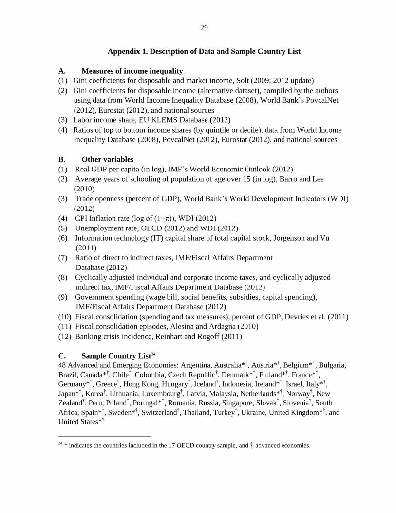
29

Appendix 1. Description of Data and Sample Country List

A. Measures of income inequality

(1) Gini coefficients for disposable and market income, Solt (2009; 2012 update)

(2) Gini coefficients for disposable income (alternative dataset), compiled by the authors

using data from World Income Inequality Database (2008), World Bank’s PovcalNet

(2012), Eurostat (2012), and national sources

(3) Labor income share, EU KLEMS Database (2012)

(4) Ratios of top to bottom income shares (by quintile or decile), data from World Income

Inequality Database (2008), PovcalNet (2012), Eurostat (2012), and national sources

B. Other variables

(1) Real GDP per capita (in log), IMF’s World Economic Outlook (2012)

(2) Average years of schooling of population of age over 15 (in log), Barro and Lee

(2010)

(3) Trade openness (percent of GDP), World Bank’s World Development Indicators (WDI)

(2012)

(4) CPI Inflation rate (log of (1+π)), WDI (2012)

(5) Unemployment rate, OECD (2012) and WDI (2012)

(6) Information technology (IT) capital share of total capital stock, Jorgenson and Vu

(2011)

(7) Ratio of direct to indirect taxes, IMF/Fiscal Affairs Department

Database (2012)

(8) Cyclically adjusted individual and corporate income taxes, and cyclically adjusted

indirect tax, IMF/Fiscal Affairs Department Database (2012)

(9) Government spending (wage bill, social benefits, subsidies, capital spending),

IMF/Fiscal Affairs Department Database (2012)

(10) Fiscal consolidation (spending and tax measures), percent of GDP, Devries et al. (2011)

(11) Fiscal consolidation episodes, Alesina and Ardagna (2010)

(12) Banking crisis incidence, Reinhart and Rogoff (2011)

C. Sample Country List34

48 Advanced and Emerging Economies: Argentina, Australia*†, Austria*†, Belgium*†, Bulgaria,

Brazil, Canada*†, Chile†, Colombia, Czech Republic†, Denmark*†, Finland*†, France*†,

Germany*†, Greece†, Hong Kong, Hungary†, Iceland†, Indonesia, Ireland*†, Israel, Italy*†,

Japan*†, Korea†, Lithuania, Luxembourg†, Latvia, Malaysia, Netherlands*†, Norway†, New

Zealand†, Peru, Poland†, Portugal*†, Romania, Russia, Singapore, Slovak†, Slovenia†, South

Africa, Spain*†, Sweden*†, Switzerland†, Thailand, Turkey†, Ukraine, United Kingdom*†, and

United States*†

34

* indicates the countries included in the 17 OECD country sample, and † advanced economies.

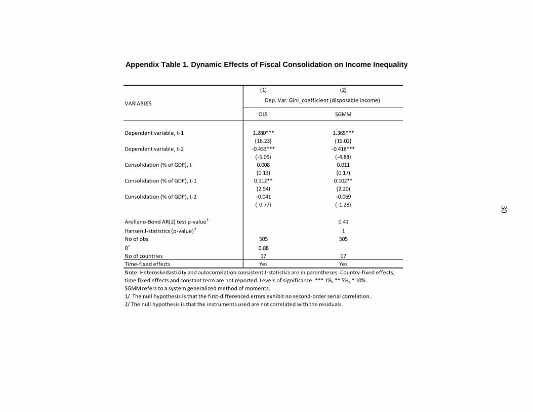
30

(1) (2)

VARIABLES

OLS SGMM

Dependent variable, t-1 1.280*** 1.365***

(16.23) (19.02)

Dependent variable, t-2 -0.433*** -0.418***

(-5.05) (-4.88)

Consolidation (% of GDP), t 0.008 0.011

(0.13) (0.17)

Consolidation (% of GDP), t-1 0.112** 0.102**

(2.54) (2.20)

Consolidation (% of GDP), t-2 -0.041 -0.069

(-0.77) (-1.28)

Arellano-Bond AR(2) test p-value1 0.41

Hansen J-statistics (p-value)2 1

No of obs 505 505

R2 0.88

No of countries 17 17

Time-fixed effects Yes Yes

SGMM refers to a system generalized method of moments.

1/ The null hypothesis is that the first-differenced errors exhibit no second-order serial correlation.

2/ The null hypothesis is that the instruments used are not correlated with the residuals.

Dep. Var: Gini_coefficient (disposable income)

Note: Heteroskedasticity and autocorrelation consistent t-statistics are in parentheses. Country-fixed effects,

time fixed effects and constant term are not reported. Levels of significance: *** 1%, ** 5%, * 10%.

Appendix Table 1. Dynamic Effects of Fiscal Consolidation on Income Inequality

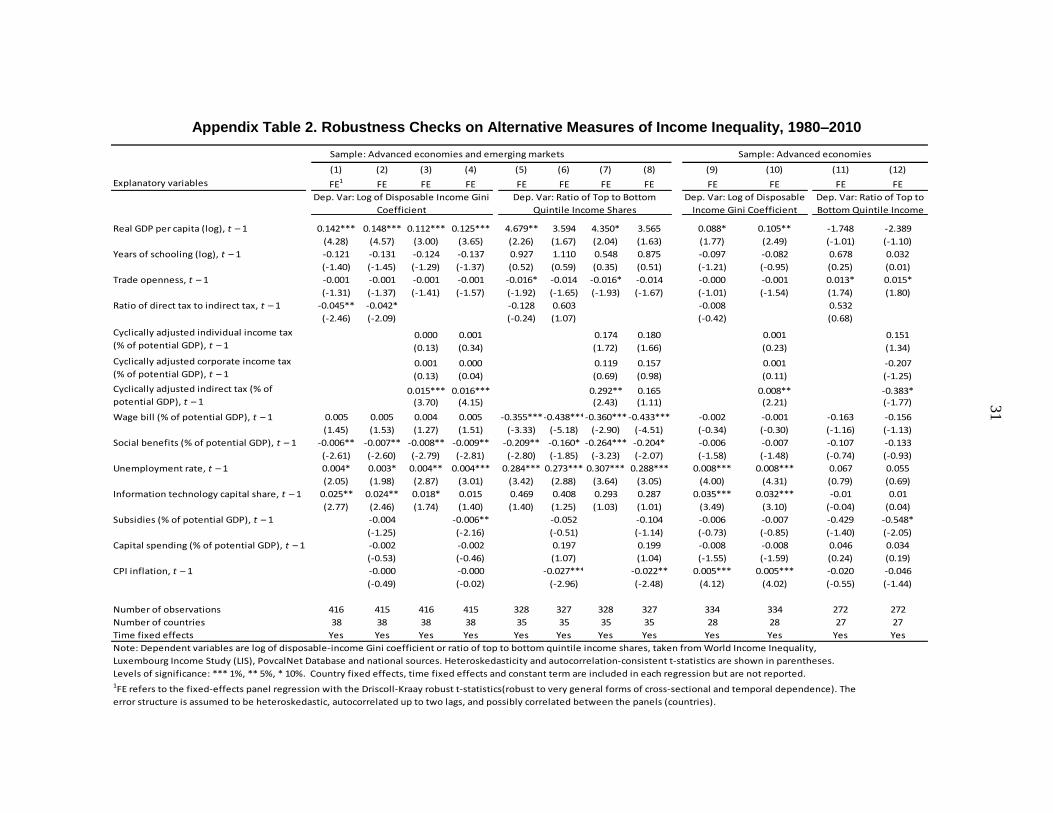
31

(1) (2) (3) (4) (5) (6) (7) (8) (9) (10) (11) (12)

Explanatory variables FE1 FE FE FE FE FE FE FE FE FE FE FE

Real GDP per capita (log), t – 1 0.142*** 0.148*** 0.112*** 0.125*** 4.679** 3.594 4.350* 3.565 0.088* 0.105** -1.748 -2.389

(4.28) (4.57) (3.00) (3.65) (2.26) (1.67) (2.04) (1.63) (1.77) (2.49) (-1.01) (-1.10)

Years of schooling (log), t – 1 -0.121 -0.131 -0.124 -0.137 0.927 1.110 0.548 0.875 -0.097 -0.082 0.678 0.032

(-1.40) (-1.45) (-1.29) (-1.37) (0.52) (0.59) (0.35) (0.51) (-1.21) (-0.95) (0.25) (0.01)

Trade openness, t – 1 -0.001 -0.001 -0.001 -0.001 -0.016* -0.014 -0.016* -0.014 -0.000 -0.001 0.013* 0.015*

(-1.31) (-1.37) (-1.41) (-1.57) (-1.92) (-1.65) (-1.93) (-1.67) (-1.01) (-1.54) (1.74) (1.80)

Ratio of direct tax to indirect tax, t – 1 -0.045** -0.042* -0.128 0.603 -0.008 0.532

(-2.46) (-2.09) (-0.24) (1.07) (-0.42) (0.68)

0.000 0.001 0.174 0.180 0.001 0.151

(0.13) (0.34) (1.72) (1.66) (0.23) (1.34)

0.001 0.000 0.119 0.157 0.001 -0.207

(0.13) (0.04) (0.69) (0.98) (0.11) (-1.25)

0.015*** 0.016*** 0.292** 0.165 0.008** -0.383*(3.70) (4.15) (2.43) (1.11) (2.21) (-1.77)

Wage bill (% of potential GDP), t – 1 0.005 0.005 0.004 0.005 -0.355***-0.438***-0.360***-0.433*** -0.002 -0.001 -0.163 -0.156

(1.45) (1.53) (1.27) (1.51) (-3.33) (-5.18) (-2.90) (-4.51) (-0.34) (-0.30) (-1.16) (-1.13)

Social benefits (% of potential GDP), t – 1 -0.006** -0.007** -0.008** -0.009** -0.209** -0.160* -0.264*** -0.204* -0.006 -0.007 -0.107 -0.133

(-2.61) (-2.60) (-2.79) (-2.81) (-2.80) (-1.85) (-3.23) (-2.07) (-1.58) (-1.48) (-0.74) (-0.93)

Unemployment rate, t – 1 0.004* 0.003* 0.004** 0.004*** 0.284*** 0.273*** 0.307*** 0.288*** 0.008*** 0.008*** 0.067 0.055

(2.05) (1.98) (2.87) (3.01) (3.42) (2.88) (3.64) (3.05) (4.00) (4.31) (0.79) (0.69)

Information technology capital share, t – 1 0.025** 0.024** 0.018* 0.015 0.469 0.408 0.293 0.287 0.035*** 0.032*** -0.01 0.01

(2.77) (2.46) (1.74) (1.40) (1.40) (1.25) (1.03) (1.01) (3.49) (3.10) (-0.04) (0.04)

Subsidies (% of potential GDP), t – 1 -0.004 -0.006** -0.052 -0.104 -0.006 -0.007 -0.429 -0.548*

(-1.25) (-2.16) (-0.51) (-1.14) (-0.73) (-0.85) (-1.40) (-2.05)

Capital spending (% of potential GDP), t – 1 -0.002 -0.002 0.197 0.199 -0.008 -0.008 0.046 0.034

(-0.53) (-0.46) (1.07) (1.04) (-1.55) (-1.59) (0.24) (0.19)

CPI inflation, t – 1 -0.000 -0.000 -0.027*** -0.022** 0.005*** 0.005*** -0.020 -0.046

(-0.49) (-0.02) (-2.96) (-2.48) (4.12) (4.02) (-0.55) (-1.44)

Number of observations 416 415 416 415 328 327 328 327 334 334 272 272

Number of countries 38 38 38 38 35 35 35 35 28 28 27 27

Time fixed effects Yes Yes Yes Yes Yes Yes Yes Yes Yes Yes Yes Yes

Dep. Var: Ratio of Top to Bottom

Quintile Income Shares

Sample: Advanced economies and emerging markets Sample: Advanced economies

Dep. Var: Log of Disposable Income Gini

Coefficient

Dep. Var: Log of Disposable

Income Gini Coefficient

Dep. Var: Ratio of Top to

Bottom Quintile Income

Note: Dependent variables are log of disposable-income Gini coefficient or ratio of top to bottom quintile income shares, taken from World Income Inequality,

Luxembourg Income Study (LIS), PovcalNet Database and national sources. Heteroskedasticity and autocorrelation-consistent t-statistics are shown in parentheses.

Levels of significance: *** 1%, ** 5%, * 10%. Country fixed effects, time fixed effects and constant term are included in each regression but are not reported.1FE refers to the fixed-effects panel regression with the Driscoll-Kraay robust t-statistics(robust to very general forms of cross-sectional and temporal dependence). The

error structure is assumed to be heteroskedastic, autocorrelated up to two lags, and possibly correlated between the panels (countries).

Cyclically adjusted individual income tax

(% of potential GDP), t – 1

Cyclically adjusted corporate income tax

(% of potential GDP), t – 1

Cyclically adjusted indirect tax (% of

potential GDP), t – 1

Appendix Table 2. Robustness Checks on Alternative Measures of Income Inequality, 1980–2010

32

References

Acemoglu, D. (2003), “Cross-Country Inequality Trends,” The Economic Journal,

113: F121–F149.

Agnello, L., and R. M. Sousa (2012), “How Does Fiscal Consolidation Impact on Income

Inequality?” Banque De France, No. 382.

Alesina, A., and S. Ardagna (2010), “Large Changes in Fiscal Policy: Taxes versus

Spending,” In: Brown, J. R. (Ed.). Tax Policy and the Economy, Vol. 24. National

Bureau of Economic Research, NBER, The University of Chicago Press.

Alesina, A., and S. Ardagna (2012), “The Design of Fiscal Adjustments”, Unpublished

Working Paper, Harvard University.

Asian Development Bank (2007), “Inequality in Asia,” In Key Indicators 2007: Inequality in

Asia, Asian Development Bank, Manila.

Atkinson, A.B., and A. Brandolini (2001), “Promise and Pitfalls in the Use of ‘Secondardy

Data-Sets: Income Inequality in OECD Countries as a Case Study,” Journal of

Economic Literature 39(3): 771-799.

Atkinson, A.B., and S. Morelli (2011), “Inequality and Banking Crises: A First Look,”

UNDP Human Development Research Paper 2011/06.

Autor, D., L. Katz, and A. Krueger (1998), “Computing Inequality: Have Computers

Changed the Labor Market?” Quarterly Journal of Economics, 1169-1213.

Ball, L., D. Leigh, and P. Loungani (2011), “Painful Medicine,” Finance and Development,

Vol 49, International Monetary Fund.

Ball, L., D. Furceri, D. Leigh, and P. Loungani (2013), “The Distributional Effects of Fiscal

Austerity,” Manuscript, International Monetary Fund.

Barones, S.J., and M.J. Alvarez-Rivadulla (2007), “Standardized Income Inequality Data for

Use in Cross-National Research,” Socio-logical Inquiry 77(1): 3-22.

Barro, R. (2008), “Inequality and Growth Revisited,” Asian Development Bank Working

Paper Series on Regional Economic Integration, No. 11, January.

Bastagli, F., D. Coady, and S. Gupta (2012), “Income Inequality and Fiscal Policy,” IMF,

Staff Discussion Note, 12/08.

33

Beck, N. and J. Katz (1995), “What to Do (and Not to Do) with Time-Series Cross-Section

Data, American Political Science Review, 89 (3): 634-647.

Berg, A., J.D. Ostry, and J. Zettelmeyer (2011), “What makes growth sustained?” European

Bank for Reconstruction and Development Working Paper No. 33, July.

BiØrn, X. (2004), “Regression Systems for Unbalanced Panel Data: A Stepwise Maximum

Likelihood Procedure,” Journal of Econometrics 122(2): 281-291.

Bruno, G. (2005), “Estimation and Inference in Dynamic Unbalanced Panel-Data Models

with a Small Number of Individuals,” Stata Journal 5(4): 473-500.

Bulir, A. (1998), “Income Inequality: Does Inflation Matters?” IMF Working Paper No 98/7.

Cerra, V., and S. Saxena. 2008. “Growth Dynamics: The Myth of Economic Recovery,”

American Economic Review, 98(1): 439–57.

Chu, K-Y., H. Davoodi, and S. Gupta (2004), “Income Distribution and Tax and Government

Social-Spending Policies in Developing Countries,” in Inequality, Growth, and

Poverty in an Era of Liberalization and Globalization, ed. by Giovanni Andrea Cornia

(New York: Oxford University Press).

Coady, D., R. Gillingham, R. Ossowski, J. Piotrowski, S. Tareq, and J. Tyson (2010),

“Petroleum Product Subsidies: Costly, Inequitable, and Rising” IMF Staff Position

Note SPN/10/05.

Cubero, R. and I. V. Hollar (2010), “Equity and Fiscal Policy: The Income Distribution

Effects of Taxation and Social Spending in Central America,” IMF Working Paper,

10/112.

Deininger, K. and L. Squire (1996), “A New Data Set Measuring Income Inequality,” World

Bank Econ Rev (1996) 10 (3): 565-591.

De Gregorio, J., and J. Lee (2002), “Education and Income Inequality: New Evidence From

Cross-Country Data,” Review of Income and Wealth, 48(3): 395-416.

Devries, P., Guajardo, J., Leigh, D., and A. Pescatori (2011), “A New Action-based Dataset

of Fiscal Consolidation,” IMF Working Paper No. 128.

Driscoll, J.C., and A.C. Kraay (1998), “Consistent Covariance Matrix Estimation with

Spatially Dependent Panel Data,” Review of Economics and Statistics, 80, 549-560.

34

Easterly, W. and S. Fisher, (2001), “Inflation and the Poor,” Journal of Money, Credit and

Banking, 1, 159-178.

Easterly, W. (2007), “Inequality Does Cause Underdevelopment: Insights from a New

Instrument,” Journal of Development Economics, 84(2), 755-776.

Gemmell, N. and O. Morrissey (2005), “Distribution and Poverty Impacts of Tax Structure

Reform in Developing Countries: How Little We Know,” Development Policy

Review, 23 (2): 131-144.

Glaeser, E. (2010), “Does Economic Inequality Cause Crises?” The New York Times, Dec

14, 2010.

Goñi, E., López, J., H. and L. Servén (2008), “Fiscal Redistribution and Income Inequality in

Latin America,” Policy Research Working Paper 4487.

IMF (2007), “Globalization and Inequality,” World Economic Outlook: 31-65.

IMF (2010a), “Appendix 3. Fiscal Adjustment and Income Distribution in Advanced and

Emerging Economies,” Fiscal Monitor, November: 94-98.

IMF (2010b), “Will It Hurt? Macroeconomic Effects of Fiscal Consolidation”, World

Economic Outlook, October.

Jorgenson, D. and K. Vu (2007), “Information Technology and the World Growth

Resurgence,” German Economic Review, 8(2): 125–145.

Joumard, I., Pisu, M., and D. Bloch (2012), “Less Income Inequality and More Growth – Are

They Compatible?: Part 3. Income Redistribution via Taxes and Transfers Across

OECD Countries,” OECD Economic Department Working Papers No. 926.

Judson, R. and A. Owen (1999), “Estimating Dynamic Panel Data Models: A Guide for

Macroeconomists," Economics Letters, 65(1): 9-15.

Kanbur, R. (2000), “Income Distribution and Development,” In A.B. Atkinson and F.

Bourguignon (editors), Handbook of Income Distribution, 791–841.

Knight, J.B. and R. Sabot (1983), “Educational Expansion and the Kuznets Effects,”

American Economic Review, 73: 1132-36.

Krugman, P. (2008), “Trade and Wages, Reconsidered,” Brookings Papers on Economic

Activity, 2: 103-137.

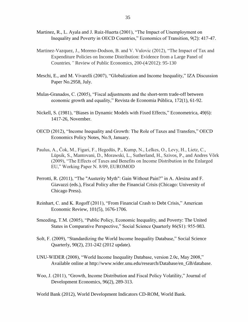
35

Martinez, R., L. Ayala and J. Ruiz-Huerta (2001), “The Impact of Unemployment on

Inequality and Poverty in OECD Countries,” Economics of Transition, 9(2): 417-47.

Martinez-Vazquez, J., Moreno-Dodson, B. and V. Vulovic (2012), “The Impact of Tax and

Expenditure Policies on Income Distribution: Evidence from a Large Panel of

Countries,” Review of Public Economics, 200-(4/2012): 95-130

Meschi, E., and M. Vivarelli (2007), “Globalization and Income Inequality,” IZA Discussion

Paper No.2958, July.

Mulas-Granados, C. (2005), “Fiscal adjustments and the short-term trade-off between

economic growth and equality,” Revista de Economia Pública, 172(1), 61-92.

Nickell, S. (1981), “Biases in Dynamic Models with Fixed Effects,” Econometrica, 49(6):

1417-26, November.

OECD (2012), “Income Inequality and Growth: The Role of Taxes and Transfers,” OECD

Economics Policy Notes, No.9, January.

Paulus, A., Čok, M., Figari, F., Hegedüs, P., Kump, N., Lelkes, O., Levy, H., Lietz, C.,

Lüpsik, S., Mantovani, D., Morawski, L., Sutherland, H., Szivos, P., and Andres Võrk

(2009), “The Effects of Taxes and Benefits on Income Distribution in the Enlarged

EU,” Working Paper N. 8/09, EUROMOD

Perrotti, R. (2011), “The "Austerity Myth": Gain Without Pain?” in A. Alesina and F.

Giavazzi (eds.), Fiscal Policy after the Financial Crisis (Chicago: University of

Chicago Press).

Reinhart, C. and K. Rogoff (2011), “From Financial Crash to Debt Crisis,” American

Economic Review, 101(5), 1676-1706.

Smeeding, T.M. (2005), “Public Policy, Economic Inequality, and Poverty: The United

States in Comparative Perspective,” Social Science Quarterly 86(S1): 955-983.

Solt, F. (2009), “Standardizing the World Income Inequality Database,” Social Science

Quarterly, 90(2), 231-242 (2012 update).

UNU-WIDER (2008), “World Income Inequality Database, version 2.0c, May 2008,”

Available online at http://www.wider.unu.edu/research/Database/en_GB/database.

Woo, J. (2011), “Growth, Income Distribution and Fiscal Policy Volatility,” Journal of

Development Economics, 96(2), 289-313.

World Bank (2012), World Development Indicators CD-ROM, World Bank.