Embed Size (px)
Citation preview
SIAM J. OPTIM. c© 2014 Society for Industrial and Applied MathematicsVol. 24, No. 3, pp. 1485–1506
DISTRIBUTIONALLY ROBUST STOCHASTIC KNAPSACKPROBLEM∗
JIANQIANG CHENG† , ERICK DELAGE‡ , AND ABDEL LISSER†
Abstract. This paper considers a distributionally robust version of a quadratic knapsack prob-lem. In this model, a subsets of items is selected to maximizes the total profit while requiring thata set of knapsack constraints be satisfied with high probability. In contrast to the stochastic pro-gramming version of this problem, we assume that only part of the information on random datais known, i.e., the first and second moment of the random variables, their joint support, and pos-sibly an independence assumption. As for the binary constraints, special interest is given to thecorresponding semidefinite programming (SDP) relaxation. While in the case that the model onlyhas a single knapsack constraint we present an SDP reformulation for this relaxation, the case ofmultiple knapsack constraints is more challenging. Instead, two tractable methods are presented forproviding upper and lower bounds (with its associated conservative solution) on the SDP relaxation.An extensive computational study is given to illustrate the tightness of these bounds and the valueof the proposed distributionally robust approach.
Key words. stochastic programming, chance constraints, distributionally robust optimization,semidefinite programming, knapsack problem
AMS subject classifications. 90C15, 90C22, 90C59
DOI. 10.1137/130915315
1. Introduction. We consider the classical quadratic knapsack problem consist-ing of the decision to include or not each of a list of n items in a bag able to carry acertain maximum weight. The “multidimensional” version of this problem takes theform of the following optimization problem
(KP ) maximizex
xTRx(1.1a)
subject to wTj x ≤ dj ∀ j ∈ {1, 2, . . . ,M},(1.1b)
xi ∈ {0, 1} ∀ i ∈ {1, 2, . . . , n},(1.1c)
where x is a vector of binary values indicating whether each item is included in theknapsack, and R ∈ �n×n is a matrix whose (i, j)th term describes the linear contribu-tion to reward of holding both items i and j. This allows us to model complementarity,when Ri,j > 0 or substitution, when Ri,j < 0, between items. Finally, for each j,wj ∈ �n is a vector of attributes (typically weights) whose total amount must satisfysome capacity constraint dj . Constraints (1.1b) are typically called knapsack con-straints and might serve to model the maximum weight or volume the bag is capableof carrying, or the fact that the total value of items that are carried must satisfysome given budget. There is a wide range of real life applications of the knapsackproblem especially in the following topics: transportation, finance, e.g. the purchaseof commodities or stocks with a limited budged, schedule planning [19]. The knapsackproblem is also used as a subproblem in several combinatorial optimization problems,
∗Received by the editors June 12, 2013; accepted for publication (in revised form) July 3, 2014;published electronically September 11, 2014.
http://www.siam.org/journals/siopt/24-3/91531.html†LRI, Universite Paris Sud, 91405, Orsay, France ([email protected], [email protected]). The first author’s
research was supported by CSC (China Scholarship Council). The third author’s research was sup-ported by HADAMARD/PGMO grant.
‡HEC Montreal, H3T2A7, Montreal, Canada ([email protected]).
1485
1486 JIANQIANG CHENG, ERICK DELAGE, AND ABDEL LISSER
e.g., cutting problems, column generation, separation of cover inequalities, knapsackcryptosystems, and combinatorial auctions [18].
In practice, it is often the case that at the time of making the knapsack decisioneither the reward parameters or the weights parameter (or both) are not exactlyknown. In that case, one has the option to represent knowledge of these parametersthrough describing a measurable space of outcomes (Ω,F) and a probability measureF on this space. The knapsack problem thus becomes a stochastic problem where Rand each wj must be considered as a randommatrix and a random vector, respectively.
Specifically, R : Ω → §R and wj : Ω → §w, with §R and §w compact convex subsetsof �n×n and �n, respectively.1 In this context, it is natural to formulate the followingstochastic program:
(SKP ) maximizex
EF [u(xT Rx)](1.2a)
subject to PF (wTj x ≤ dj ∀ j ∈ {1, . . . ,M}) ≥ 1− η,(1.2b)
xi ∈ {0, 1} ∀ i ∈ {1, 2, . . . , n}(1.2c)
for some concave utility function u(·) that captures risk aversion with respect to thetotal achieved reward. In this formulation, the knapsack constraints are required tobe jointly met with probability larger than 1− η for some small η.
Under many circumstances, the assumption of full knowledge of the distributionF fails. For this reason, it can be necessary to consider that the only knowledge wehave of a distribution is that it is part of some uncertainty set D. Following a robustapproach, in this context we might be interested in choosing items for our knapsackso that the value of the knapsack, as measured by the stochastic program, has thebest worst-case guarantees under the choice of a distribution in this uncertainty set.Hence, our interest lies in solving:
(DRSKP ) maximizex
infF∈D
EF [u(xT Rx)](1.3a)
subject to infF∈D
PF (wTj x ≤ dj ∀ j ∈ {1, 2, . . . ,M}) ≥ 1− η,(1.3b)
xi ∈ {0, 1} ∀ i ∈ {1, 2, . . . , n}.(1.3c)
In this paper, we consider a distributionally robust stochastic knapsack problem,where we assume that only part of the information on random data is known. Forthe knapsack problem with a single knapsack constraint, when information is limitedto mean, covariance, and support of the uncertain data, we show that the (DRSKP)problem reduces to a semidefinite program (SDP) after applying the SDP based relax-ation scheme to the binary constraints. To the best of our knowledge, this is the firsttime that an SDP representation is derived for distributionally robust chance con-straints where both first and second moments and support are known. Unfortunately,this reformulation does not extend to multidimensional knapsack problems whereM > 1. Therefore, for the more general form, after relaxing the binary constraintswith some common linear matrix inequality, we study the case here information islimited to the distribution’s first and second moments and some form of indepen-dence and propose efficient approximations that provide both a lower bound and an
1Note that d is assumed certain without loss of generality since one can always capture such un-certainty by including an additional decision x0 that absolutely needs to be included in the knapsackand a set of random weights (wj)0.
DISTRIBUTIONALLY ROBUST STOCHASTIC KNAPSACK 1487
upper bound for the model. As a side product, a conservative solution to the re-laxed problem is obtained. An extensive computational study is provided to illustratethe tightness of these bounds and the value of the proposed distributionally robustapproach.
The rest of the paper is organized as follows. In section 2, we review recent work onthe topic of stochastic and robust knapsack problems. In section 3, we describe in moredetails the distributionally robust stochastic knapsack problem (DRSKP) with singleknapsack constraint and introduce its SDP relaxation. Later, in section 4, we proposetwo approximation methods for the DRSKP with multiple knapsack constraints, alsoreferred to as a multidimensional knapsack problem. Finally, in section 5, we reportour numerical experiments and section 6 summarizes our results.
Remark 1.1. Note that one can show that solving (DRSKP) is equivalent tosolving
(1.4) maximizex∈{0,1}n
infF∈D
SKP(x, F ),
where SKP(x, F ) refers to the objective function of this problem that is augmentedwith feasibility verification, i.e.,
SKP(x;F ) =
{EF [u(x
T Rx)] if PF (wTj x ≤ dj ∀ j ∈ {1, 2, . . . ,M}) ≥ 1− η,
−∞ otherwise..
This is simply due to the fact that in order for infF∈D SKP(x, F ) to be finite valued,x must satisfy constraint (1.3b).
2. Prior work. The binary quadratic knapsack problem (QKP) was first intro-duced by Gallo et al. [12]. Since then, there has been an extensive literature on QKPand its various aspects [3, 4, 6, 24]. Gallo, Hammer, and Simeone [12] invented QKPand gave a family of upper bounds based on upper planes. Martello and Toth [24] gavea pseudo-polynomial-time algorithm. Johnson, Mehrotra, and Nemhauser [16] consid-ered a graph version of the QKP and solved it by a branch-and-cut system. Billionnetand Calmels [3] used a classical linearization technique of the objective function toobtain an integer linear program formulation. Due to different uncertainty factors,the parameters are not known in advance. Then, it is natural to model the problemas a stochastic problem. For more information about the stochastic knapsack prob-lem, we refer the reader to [11, 19, 20, 23, 33] and references therein. The knapsackproblem has also been studied under the lens of robust optimization. In [17], it wasestablished that the problem is strongly NP-hard even when the uncertainty is limitedto the objective function and the uncertainty set is composed of a finite number ofscenarios. More recently, in [21] the authors considered a min-max knapsack problemthat was specifically designed to solve the chance-constrained problem and proposed asolution method whose complexity again grew exponentially in the size of the scenarioset. In an attempt to circumvent the computational challenge, Bertsimas and Sim [1]identified an uncertainty set, referred to as being “budgeted,” that allowed a mixedinteger linear programming reformulation for robust combinatorial problems like theknapsack, thus amenable to be solved by powerful available algorithms such as inCPLEX [15]. In [25], the authors provided tight bounds on the price of robustness ofknapsack problems, i.e. relative cost increase for using a solution that was feasible forall weight perturbations. To the best of our knowledge, there is no prior work study-ing the application of distributionally robust optimization to the stochastic quadraticknapsack (or multidimensional knapsack) problem.

1488 JIANQIANG CHENG, ERICK DELAGE, AND ABDEL LISSER
The concept of distributionally robust optimization was initially introduced in1958 by Scarf [27] who named the method minimax stochastic programming. Whilethe original application was a single item newsvendor problem, the range of appli-cations of this method was rather limited due to numerical difficulties encounteredwhen solving large instances. Recently, mainly due to the development of efficientinterior point algorithms for solving SDPs and perhaps also because of the new “dis-tributionally robust” branding, the method has become very popular. In [9], theauthors showed that a large range of distributionally robust optimization models,where the distribution’s mean and covariance matrix were constrained, can be solvedin polynomial time, and were often equivalent to an SDP reformulation. In [5], theframework was applied to address chance constraints which were typically consideredas an intractable construct when the distribution was assumed to be known. BothChen et al. [7] and Zymler, Kuhn, and Rustem [34], extended this work to provideapproximations when chance constraints were joint (i.e. constraints must be satisfiedjointly with high probability). Recently, the work in [32] has shed even more light onthe range of functions and uncertainty sets that can be addressed using SDP.
Unfortunately, to this day, the application of distributionally robust optimizationto integer programs has been rather scarce. In [2], the authors sought bounds forthe worst-case objective function value of stochastic integer programs when only mo-ments were known about the distribution. In [22], the authors considered a schedulingproblem where the integer decision variables were the number of employees assignedto different schedules. They considered uncertainty in scenario probabilities and usedpolyhedral uncertainty sets to preserve the mixed integer linear programming struc-ture of the nominal problem. Most closely related to our work is the work by Wagnerin [30] who studied a stochastic 0-1 linear program with chance constraints wheredistribution information was limited to moments up to order k. He presented how toaddress this problem using a hierarchy of SDPs with integer constraints. Compara-tively, we address a stochastic 0-1 quadratic program and consider the joint chanceconstraint in the case of a multidimensional knapsack.
3. Distributionally robust knapsack problem. There are two difficultiesthat need to be addressed when searching for the optimal solution of the DRSKPproblem. First, the worst-case analysis that is needed to evaluate the objective andverify the chance constraint involves optimization over an infinite dimensional de-cision space. Second, the problem is intrinsically a combinatorial one. In this sec-tion, we provide an approximation for the distributionally robust knapsack problemwith a single knapsack constraint, i.e., M = 1. This approximation will be basedon an exact reformulation of problem (1.3) as a finite dimensional SDP problemwith binary variables. We will then relax the binary constraints using linear matrixinequalities.
3.1. Finite dimensional reformulation. We start our study by making asmall set of assumptions. These will be needed to ensure that the approximationmodel we obtain can be solved efficiently.
Definition 3.1. Let ξ be a random vector in �m on which R and w1 (referredto henceforth as w) depend linearly:
R =
m∑i=1
ARi ξi, w = Awξ.

DISTRIBUTIONALLY ROBUST STOCHASTIC KNAPSACK 1489
Assumption 3.2. The utility function u(·) is piecewise linear, increasing, andconcave. In other words, it can be represented in the form
u(y) = mink∈{1,2,...,K}
aky + bk,
where a ∈ �K and a ≥ 0.Assumption 3.3. The distributional uncertainty set accounts for information
about the convex support §, mean μ in the strict interior of §, and an upper boundΣ 0 on the covariance matrix of the random vector ξ:
D(§, μ,Σ) =
⎧⎪⎨⎪⎩F
∣∣∣∣∣∣∣P(ξ ∈ §) = 1
EF [ξ] = μ
EF [(ξ − μ)(ξ − μ)T ] Σ
⎫⎪⎬⎪⎭ .
Definition 3.1 is made without loss of generality since we can always consider ξto contain all the terms of R and w. On the other hand, regarding Assumption 3.2,although piecewise-linear utility functions are not the common functions to use whenapplying expected utility theory, they provide enough flexibility to approximate to ahigh level of accuracy any function that one might be interested in using. Finally, As-sumption 3.3 implies that one only knows the support of R and w (or a set containingthis support), the mean of these random terms, and some information about varianceand covariance. We refer the reader to [9] for a full discussion about this choice ofdistributional uncertainty, in particular for the use of a linear matrix inequality tocapture information about the covariance matrix.
Theorem 3.4. Under Assumptions 3.2 and 3.3, and given that § is compact andM = 1, then the following deterministic problem
(3.1a)
maximizex,t,q,Q,t,q,Q,s
t− μTq− (Σ + μμT ) •Q
(3.1b)
subject to t ≤m∑j=1
ak ξjxTAR
j x+ bk + ξTq+ ξTQξ ∀ξ ∈ § ∀k = {1, . . . ,K},
t+ 2μT q+ (Σ + μμT ) • Q ≤ ηs,(3.1c)
t+ 2ξT q+ ξT Qξ ≥ 0 ∀ ξ ∈ §,(3.1d)
t+ 2ξT q+ ξT Qξ − s+ 2d− 2ξTAwTx ≥ 0 ∀ ξ ∈ §,(3.1e)
Q � 0, Q � 0, s ≥ 0,(3.1f)
xi ∈ {0, 1} ∀i ∈ {1, 2, . . . , n},(3.1g)
where t, t ∈ �, q, q ∈ �m, Q, Q ∈ �m×m, s ∈ �, and • is the Frobenius inner productdefined by A•B =
∑i,j AijBij , where A and B are two conformal matrices, identifies
a solution x∗ that is guaranteed to be feasible for problem (1.3) and to perform at leastas well in terms of the objective function as an optimal solution of problem (1.3) withd1 replaced by d1 − ε for any ε > 0.
Remark 3.5. In practice, one might actually consider that the solution of prob-lem (3.1) is the solution that one is looking for given that dj is a continuous parameter

1490 JIANQIANG CHENG, ERICK DELAGE, AND ABDEL LISSER
and could have easily been slightly overestimated (and similarly E[w] might have beenunderestimated).
Proof. The proof relies here on applying the theory presented in [9] to convertthe distributionally robust objective into its deterministic equivalent. This gives riseto the reformulated objective function in terms of auxiliary variables t, q, and Q, andconstraint (3.1b). In a second step, one can adapt the ideas used to prove Theorem1 of [10] to an uncertainty set that account for the first and second moments and thesupport constraints presented in Assumption 3.3. The key idea here will be to replaceconstraint (1.3b) with
infF∈(§,μ,Σ)
PF (ξTAwT
x < d) ≥ 1− η,
which is both stricter than the original one and more relaxed than
infF∈(§,μ,Σ)
PF (ξTAwT
x ≤ d− ε) ≥ 1− η
for any ε > 0. This new constraint is equivalent to verifying that the optimal valueof the following infinite dimensional problem is not greater than η:
supF∈(§,μ,Σ)
EF [�{ξTAwTx ≥ d}],
where �{·} is the indicator function that gives one if the statement is verified andzero otherwise. By duality theory (see [9]), this problem is equivalent to
minimizet,q,Q
t+ 2μT q+ (Σ + μμT ) • Q
subject to − �{ξTAwTx ≥ d}+ t+ 2ξT q+ ξT Qξ ≥ 0 ∀ ξ ∈ §,
Q � 0,
where t ∈ �, q ∈ �m, and Q ∈ �m×m. One can show that duality is strict since theconditions laid out in Assumption 3.3 ensure that the Dirac measure δμ lies in therelative interior of the distributional set, hence the weaker version of Proposition 3.4in [28] applies.
When M = 1, we get that constraint (1.3b) can be reformulated as
t+ 2μT q+ (Σ + μμT ) • Q ≤ η,(3.2a)
t+ 2ξT q+ ξT Qξ ≥ 0 ∀ ξ ∈ §,(3.2b)
−1 + t+ 2ξT q+ ξT Qξ ≥ 0 ∀ ξ ∈ § ∩ {ξ ∈ �m|ξTAwTx ≥ d}.(3.2c)
Studying more closely the third constraint, one realizes that it can be expressed as
minξ∈§
supλ≥0
−1 + t+ 2ξT q+ ξT Qξ + 2λ(d− ξTAwTx) ≥ 0,
which by Sion’s minimax theorem, since § is compact and Q is positive semidefinite,is equivalent to
supλ≥0
minξ∈§−1 + t+ 2ξT q+ ξT Qξ + 2λ(d− ξTAwT
x) ≥ 0.
DISTRIBUTIONALLY ROBUST STOCHASTIC KNAPSACK 1491
Again since § is compact, this constraint can be replaced by
supλ>0
minξ∈§−1 + t+ 2ξT q+ ξT Qξ + 2λ(d− ξTAwT
x) ≥ 0,
which can be reformulated as
supλ>0
minξ∈§−1/λ+ (1/λ)t+ 2(1/λ)ξT q+ (1/λ)ξT Qξ + 2(d− ξTAwT
x) ≥ 0.
The three constraints can therefore be restated as
(1/λ)t+ 2(1/λ)μT q+ (Σ + μμT ) • (1/λ)Q ≤ η(1/λ),
(1/λ)t+ 2(1/λ)ξT q+ (1/λ)ξT Qξ ≥ 0 ∀ ξ ∈ §,−(1/λ) + (1/λ)t+ 2(1/λ)ξT q+ (1/λ)ξT Qξ + 2(d− ξTAwT
x) ≥ 0 ∀ ξ ∈ §.
A simple replacement of variables s := (1/λ), t′ := (1/λ)t, q′ := (1/λ)q, and Q′ :=(1/λ)Q leads to constraints (3.1c), (3.1d), (3.1e).
It is important to realize that while many ideas behind this result are drawn fromthe existing litterature on distributionally robust optimization, to the best of ourknowledge the proposed reformulation for a distributionally robust chance constraintthat accounts for both first and second moment and support information appears forthe first time and should be of interest in other fields of application. The key inobtaining this result is in exploiting the structure of EF [(ξ − μ)(ξ − μ)T ] Σ, aswas done in [9], which ensures that Q and Q are positive-semidefinite matrices. Thisproperty enables the use of conic duality to reformulate constraint (3.2c) instead ofusing an approximate version of the S-lemma.
While problem (3.1) still takes the form of an infinite dimensional problem, ifthe support set § is representable by a set of linear matrix inequalities, then one caneasily obtain the robust counterparts of constraints (3.1b), (3.1d), and (3.1e). Next,we present three natural examples.
Corollary 3.6. Given that the support of F is ellipsoidal, § ={ξ|(ξ − ξ0)
TΘ(ξ − ξ0) ≤ 1}, problem (1.4) further reduces to the following problem
maximizex,t,q,Q,v,s,t,q,Q,s
t− μTq− (Σ + μμT ) •Q(3.3a)
subject to
[Q q+akv
2
qT+akvT
2 bk − t
]� −sk
[Θ −Θξ0
−ξT0 Θ ξT0 Θξ0 − 1
]∀ k,(3.3b)
vj = ARj • (xxT )∀ j ∈ {1, 2, . . . ,m},(3.3c)
t+ 2μT q+ (Σ + μμT ) • Q ≤ ηs1,(3.3d) [Q q
qT t
]� −s2
[Θ −Θξ0
−ξT0 Θ ξT0 Θξ0 − 1
],(3.3e)
[Q q−AwT
x
(q−AwTx)T t+ 2d− s1
]� −s3
[Θ −Θξ0
−ξT0 Θ ξT0 Θξ0 − 1
],(3.3f)
Q � 0, Q � 0, s ≥ 0, s ≥ 0,(3.3g)
xi ∈ {0, 1} ∀i ∈ {1, 2, . . . , n}.(3.3h)

1492 JIANQIANG CHENG, ERICK DELAGE, AND ABDEL LISSER
Alternatively, if the support of F is polyhedral, i.e., § = {ξ|Cξ ≤ c} with C ∈ �p×m
and c ∈ �p, then problem (1.4) reduces to
maximizex, t,q,Q,v, s, t, q, Qλ1, λ2, . . . , λK + 2
t− μTq− (Σ + μμT ) •Q
subject to
⎡⎣ Q q+akv+CTλk
2
qT+akvT+λT
k C2 bk − t− cTλk
⎤⎦ � 0 ∀ k
vj = ARj • (xxT ) ∀ j ∈ {1, 2, . . . ,m},
t+ 2μT q+ (Σ + μμT ) • Q ≤ ηs,[Q q+ 1
2CTλK+1
qT + 12λ
TK+1C t− cTλK+1
]� 0,
⎡⎣ Q q−AwT
x+ 12C
TλK+2
(q−AwTx)T + 1
2λTK+2C t+ 2d− s− cTλK+2
⎤⎦ � 0,
Q � 0, Q � 0, s ≥ 0, λk ≥ 0 ∀k ∈ {1, 2, . . . ,K + 2},xi ∈ {0, 1} ∀i ∈ {1, 2, . . . , n},
where λk ∈ �p for all k are the dual variables associated with the linear inequalitiesCξ ≤ c for each infinite set of constraints. Finally, if the support of F is unbounded(i.e. § = �m), then problem (1.4) reduces to
maximizex,t,q,Q,v,z,τ
t− μTq− (Σ + μμT ) •Q(3.4a)
subject to
[Q q+akv
2
qT+akvT
2 bk − t
]� 0 ∀ k = {1, 2, . . . ,K},(3.4b)
vj = ARj • (xxT ) ∀ j ∈ {1, 2, . . . ,m},(3.4c)
Q � 0, τk ≥ 0 ∀ k = {1, 2, . . . ,K},(3.4d) [0m,m Σ1/2z
zTΣ1/2 0
]�√
η
1− η(μT z− d)I,(3.4e)
z = AwTx,(3.4f)
xi ∈ {0, 1} ∀i ∈ {1, 2, . . . , n}.(3.4g)
Proof. In the case of the spherical support, the proof simply relies on applyingthe S-Lemma (see [26] for details) on each infinite set of constraints (3.1b), (3.1d),and (3.1e). Otherwise, with the polyhedral set, since Q and Q are positive semi-definite, one can easily apply duality theory to construct the so-called robust coun-terpart of each constraint that is indexed by ξ ∈ §. Finally, although the support setis not compact when § = �m, duality theory can still be applied and the reductionsneeded for the worst-case expected cost and worst-case chance constraint have beenpresented in [9] and [10].
Example 3.7. For clarity, we present an example in which problem (3.1) returnsa conservative solution for problem (1.3) that we argue might actually be the solutionthat a practitioner should implement. Consider a knapsack problem with a single item

DISTRIBUTIONALLY ROBUST STOCHASTIC KNAPSACK 1493
with weight in the range [0, 2] with an expected value estimated to be 1 and standarddeviation of 1. The question is whether to put the item in the knapsack or not giventhat we wish to have at least 90% confidence that the total weight will be less than orequal to 2, i.e. the maximum weight the knapsack can hold. It is clear here that theoptimal solution of problem (1.3) is to wrap the item in the knapsack thus giving fullconfidence that the total weight will be less than or equal to 2. Yet, since problem (3.1)is derived after changing the maximum total weight constraint to a strict inequalityin the chance constraint, it will consider that the optimal solution is to leave the itemout of the knapsack since in the worst case there is a 50% chance that the weightis exactly 2. This approximate solution is feasible in terms of problem (1.3) andperforms at least as well as the optimal solution of all versions of the problem wherethe maximum total weight that is considered is strictly smaller than two. Since theworst-case distribution for the solution that wraps the item up has 50% probabilitythat the knapsack will carry exactly its estimated maximum load, in practice thesolution of leaving the item aside is potentially the better one considering that it isbetter protected against estimation error.
3.2. Semidefinite programming approximation. In order to obtain an ap-proximation model with known polynomial convergence rate, we apply an SDP basedrelaxation scheme to the binary constraints. This scheme makes use of a liftingthrough the decision matrix X:
X = xxT .
As what is commonly done for combinatorial problems, we start by imposing theredundant constraints
Xi,j ≥ 0 ∀ i, j & Xi,i = xi ∀ i,since xixj ≥ 0 and x2
i = xi when xi is either zero or one.We then relax the nonconvex constraint X = xxT to X � xxT which can take
the form of a linear matrix inequality.[X x
xT 1
]� 0.
When the support set is ellipsoidal, we have the following SDP problem:
maximizex,t,q,Q,v,s,t,q,Q,s
t− μTq− (Σ + μμT ) •Q
(3.5a)
subject to
[Q q+akv
2
qT+akvT
2 bk − t
]� −sk
[Θ −Θξ0
−ξT0 Θ ξT0 Θξ0 − 1
]∀ k,(3.5b)
vj = ARj •X ∀ j ∈ {1, 2, . . . ,m},(3.5c)
t+ 2μT q+ (Σ + μμT ) • Q ≤ ηs1,(3.5d) [Q q
qT t
]� −s2
[Θ −Θξ0
−ξT0 Θ ξT0 Θξ0 − 1
],(3.5e)
[Q q−AwT
x
(q−AwTx)T t+ 2d− s1
]� −s3
[Θ −Θξ0
−ξT0 Θ ξT0 Θξ0 − 1
],(3.5f)

1494 JIANQIANG CHENG, ERICK DELAGE, AND ABDEL LISSER
Q � 0, Q � 0, s ≥ 0, s ≥ 0,(3.5g) [X x
xT 1
]� 0,(3.5h)
Xi,i = xi ∀ i, Xi,j ≥ 0 ∀ i, j,(3.5i)
where we removed constraint 0 ≤ x ≤ 1 given that it is already imposed throughconstraints (3.5h) and (3.5i).
4. Multidimensional knapsack problem. Here we consider a distributionallyrobust approach to stochastic multidimensional knapsack problems. To make thissection self-contained, we recall that the DRSKP is formulated as
maximizex
infF∈D
EF [u(xT Rx)](4.1a)
subject to infF∈D
PF (wTj x ≤ dj , j = 1, . . . ,M) ≥ 1− η,(4.1b)
xi ∈ {0, 1} ∀ i ∈ {1, 2, . . . , n}(4.1c)
for some piecewise linear concave increasing utility function u(·), where F now de-scribes the joint distribution of all types of “weights” of all items, {wj}Mj=1 ∼ F , andD now describes a set of such joint distributions.
Definition 4.1. Without loss of generality, for all j = 1, . . . ,M , let ξj be a
random vector in �m on which the wj depend linearly and let R depend linearly on{ξj}Mj=1:
R =M∑j=1
m∑i=1
ARji(ξj)i, wj = A
wj
j ξj , j = 1, . . . ,M.
Assumption 4.2. The distributional uncertainty set accounts for informationabout the mean μj , and an upper bound Σj on the covariance matrix of the randomvector ξj , for each j = 1, . . . ,M :
D(μj ,Σj) =
{Fj
∣∣∣∣∣EFj [ξj ] = μj
EFj [(ξj − μj)(ξj − μj)T ] Σj
}.
Furthermore, the random vectors ξi and ξj are independent when i �= j. Note thatthe support of Fj is unbounded, i.e. § = �m.
Theorem 4.3. Under Assumptions 3.2 and 4.2, the following problem is a con-servative approximation2 of problem (4.1):
(4.2a)
maximizex,t,q,Q,v
t− μTq− (Σ + μμT ) •Q(4.2b)
subject to
[Q q+akv
2
qT+akvT
2 bk − t
]� 0 ∀ k = {1, 2, . . . ,K},
2The concept of conservative approximation denotes the fact that the solution to the approximatemodel is guaranteed to achieve an expected utility that is at least as large as the obtained approximateoptimal objective value.
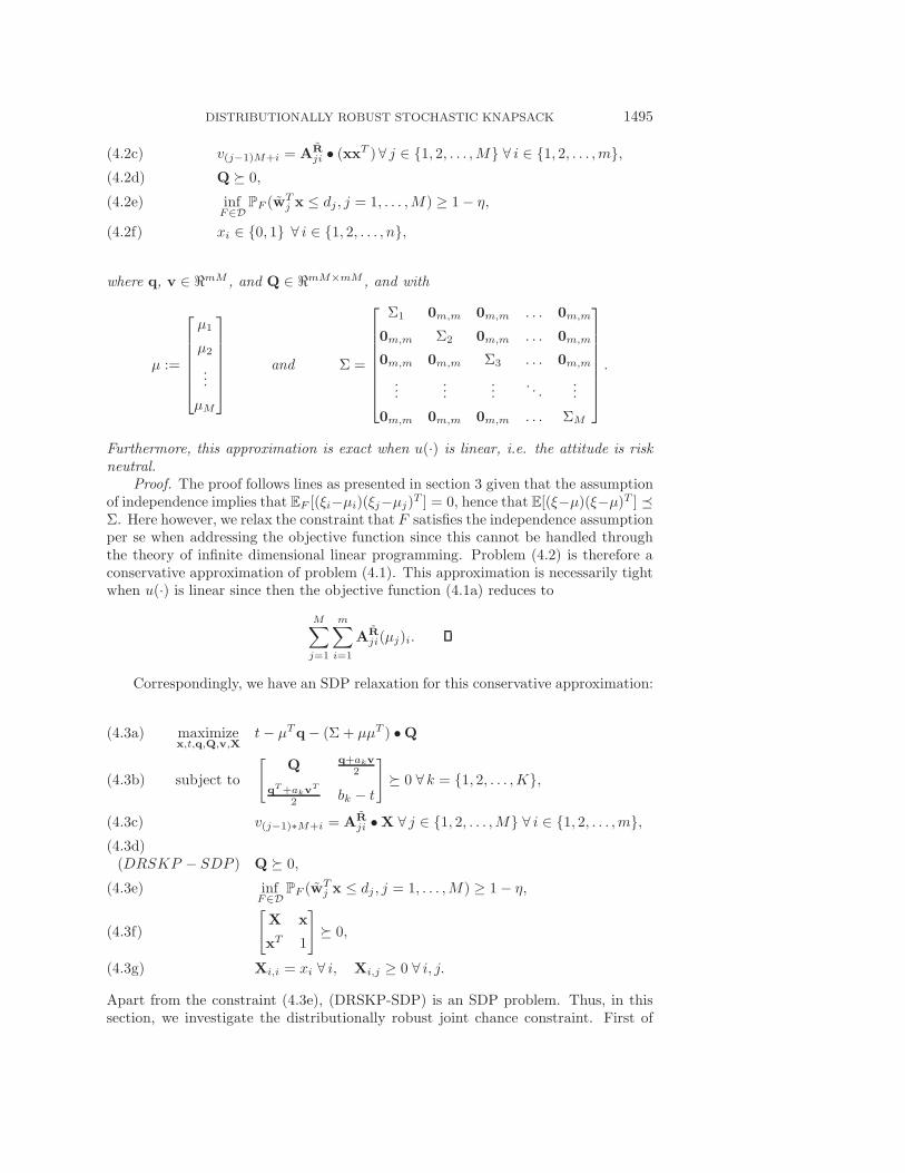
DISTRIBUTIONALLY ROBUST STOCHASTIC KNAPSACK 1495
v(j−1)M+i = ARji • (xxT )∀ j ∈ {1, 2, . . . ,M} ∀ i ∈ {1, 2, . . . ,m},(4.2c)
Q � 0,(4.2d)
infF∈D
PF (wTj x ≤ dj , j = 1, . . . ,M) ≥ 1− η,(4.2e)
xi ∈ {0, 1} ∀ i ∈ {1, 2, . . . , n},(4.2f)
where q, v ∈ �mM , and Q ∈ �mM×mM , and with
μ :=
⎡⎢⎢⎢⎢⎢⎣
μ1
μ2
...
μM
⎤⎥⎥⎥⎥⎥⎦ and Σ =
⎡⎢⎢⎢⎢⎢⎢⎢⎣
Σ1 0m,m 0m,m . . . 0m,m
0m,m Σ2 0m,m . . . 0m,m
0m,m 0m,m Σ3 . . . 0m,m
......
.... . .
...
0m,m 0m,m 0m,m . . . ΣM
⎤⎥⎥⎥⎥⎥⎥⎥⎦.
Furthermore, this approximation is exact when u(·) is linear, i.e. the attitude is riskneutral.
Proof. The proof follows lines as presented in section 3 given that the assumptionof independence implies that EF [(ξi−μi)(ξj−μj)
T ] = 0, hence that E[(ξ−μ)(ξ−μ)T ] Σ. Here however, we relax the constraint that F satisfies the independence assumptionper se when addressing the objective function since this cannot be handled throughthe theory of infinite dimensional linear programming. Problem (4.2) is therefore aconservative approximation of problem (4.1). This approximation is necessarily tightwhen u(·) is linear since then the objective function (4.1a) reduces to
M∑j=1
m∑i=1
ARji(μj)i.
Correspondingly, we have an SDP relaxation for this conservative approximation:
maximizex,t,q,Q,v,X
t− μTq− (Σ + μμT ) •Q(4.3a)
subject to
[Q q+akv
2
qT+akvT
2 bk − t
]� 0 ∀ k = {1, 2, . . . ,K},(4.3b)
v(j−1)∗M+i = ARji •X ∀ j ∈ {1, 2, . . . ,M} ∀ i ∈ {1, 2, . . . ,m},(4.3c)
(DRSKP − SDP ) Q � 0,(4.3d)
infF∈D
PF (wTj x ≤ dj , j = 1, . . . ,M) ≥ 1− η,(4.3e) [
X x
xT 1
]� 0,(4.3f)
Xi,i = xi ∀ i, Xi,j ≥ 0 ∀ i, j.(4.3g)
Apart from the constraint (4.3e), (DRSKP-SDP) is an SDP problem. Thus, in thissection, we investigate the distributionally robust joint chance constraint. First of

1496 JIANQIANG CHENG, ERICK DELAGE, AND ABDEL LISSER
all, we review two lower bounding (also referred to as “conservative”) approximationsthat have recently been proposed in the literature. We then introduce two novelapproximations for lower bounding and upper bounding the value of (DRSKP-SDP)which will exploit the structure of the joint chance constraint under our independenceassumption.
4.1. Bonferroni’s conservative bound. A popular approximation for jointchance-constrained problems is based on Bonferroni’s inequality, which decomposesthe joint constraint into M individual constraints. When
∑Mj=1 ηj = η for any F ,
we have
PF (wTj x ≤ dj) ≥ 1− ηj , j = 1, . . . ,M ⇒ PF (w
Tj x ≤ dj , j = 1, . . . ,M) ≥ 1− η.
One can already obtain from this fact a trivial conservative approximation for the(DRSKP-SDP) problem.
Theorem 4.4. The (DRSKP-SDP) problem with constraint (4.3e) replaced with[0m,m Σ
1/2j zj
zTj Σ1/2j 0
]�√
ηj1− ηj
(μTj zj − dj)I ∀ j = 1, . . . ,M,
zj = Awj
j
Tx ∀ j = 1, . . . ,M,
where zj ∈ �m are additional auxiliary decision variables, is an SDP problem. Theoptimal solution of this SDP is feasible according to the original (DRSKP-SDP) andits optimal value provides a lower bound on the value of the original problem.
4.2. Zymler, Kuhn, and Rustem’s conservative bound. In [34], the au-thors address the distributionally robust chance constraint by introducing a scalingparameter α ∈ A = {α ∈ �M : α > 0} and reformulating it as a distributionallyrobust value-at-risk constraint. For any α ∈ A
infF∈D
PF (wTj x ≤ dj , j = 1, . . . ,M) ≥ 1− η
⇔ infF∈D
PF
(max
j{αj(w
Tj x− dj)} ≤ 0
)≥ 1− η
⇔ infF∈D
VaR-ηF
(max
j{αj(w
Tj x− dj)}
)≤ 0.
The next step involves replacing the value-at-risk operator by an upper boundingconditional value-at-risk operation to make it both convex and tractable. For anyα > 0, this leads to the following conservative approximation of (DRSKP-SDP). Werefer the reader to [34] for more details.
Theorem 4.5. Consider the (DRSKP-SDP) problem with constraint (4.3e) re-placed by
β +1
η
[Σ+ μμT 1
2μ
12μ
T 1
]•M ≤ 0,
M−[0mM,mM
12αjyj
12αjy
Tj −αjdj − β
]� 0 ∀j = 1, . . . ,M,
yj =[0(j−1)m
T xTAjwj 0(M−j)m
T]T
,
M� 0,
DISTRIBUTIONALLY ROBUST STOCHASTIC KNAPSACK 1497
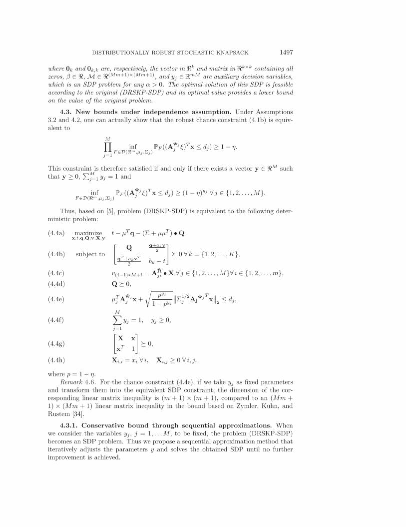
where 0k and 0k,k are, respectively, the vector in �k and matrix in �k×k containing allzeros, β ∈ �,M ∈ �(Mm+1)×(Mm+1), and yj ∈ R
mM are auxiliary decision variables,which is an SDP problem for any α > 0. The optimal solution of this SDP is feasibleaccording to the original (DRSKP-SDP) and its optimal value provides a lower boundon the value of the original problem.
4.3. New bounds under independence assumption. Under Assumptions3.2 and 4.2, one can actually show that the robust chance constraint (4.1b) is equiv-alent to
M∏j=1
infF∈D(�m,μj ,Σj)
PF ((Awj
j ξ)Tx ≤ dj) ≥ 1− η.
This constraint is therefore satisfied if and only if there exists a vector y ∈ �M suchthat y ≥ 0,
∑Mj=1 yj = 1 and
infF∈D(�m,μj ,Σj)
PF ((Awj
j ξ)Tx ≤ dj) ≥ (1− η)yj ∀ j ∈ {1, 2, . . . ,M}.
Thus, based on [5], problem (DRSKP-SDP) is equivalent to the following deter-ministic problem:
maximizex,t,q,Q,v,X,y
t− μTq− (Σ + μμT ) •Q(4.4a)
subject to
[Q q+akv
2
qT+akvT
2 bk − t
]� 0 ∀ k = {1, 2, . . . ,K},(4.4b)
v(j−1)∗M+i = ARji •X ∀ j ∈ {1, 2, . . . ,M}∀ i ∈ {1, 2, . . . ,m},(4.4c)
Q � 0,(4.4d)
μTj A
wj
j x+
√pyj
1− pyj
∥∥Σ1/2j Aj
wjTx∥∥2≤ dj ,(4.4e)
M∑j=1
yj = 1, yj ≥ 0,(4.4f)
[X x
xT 1
]� 0,(4.4g)
Xi,i = xi ∀ i, Xi,j ≥ 0 ∀ i, j,(4.4h)
where p = 1− η.Remark 4.6. For the chance constraint (4.4e), if we take yj as fixed parameters
and transform them into the equivalent SDP constraint, the dimension of the cor-responding linear matrix inequality is (m + 1) × (m + 1), compared to an (Mm +1) × (Mm + 1) linear matrix inequality in the bound based on Zymler, Kuhn, andRustem [34].
4.3.1. Conservative bound through sequential approximations. Whenwe consider the variables yj , j = 1, . . .M , to be fixed, the problem (DRSKP-SDP)becomes an SDP problem. Thus we propose a sequential approximation method thatiteratively adjusts the parameters y and solves the obtained SDP until no furtherimprovement is achieved.
1498 JIANQIANG CHENG, ERICK DELAGE, AND ABDEL LISSER
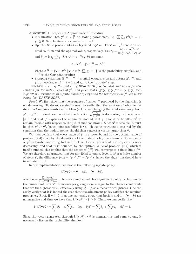
Algorithm 1. Sequential Approximation Procedure.• Initialization: Let y1 ∈ RM
+ be scaling parameters, i.e.,∑M
j=1 y1(j) = 1,
y1 ≥ 0. Set the iteration counter to t := 1.• Update: Solve problem (4.4) with y fixed to yt and let xt and f t denote an op-
timal solution and the optimal value, respectively. Let zj =(dj−μT A
wjj xt)2
(‖Σ1/2j Aj
wjTxt‖2)2
and ytj = logpzj
zj+1 . Set yt+1 ← U(y; y) for some
U : ΔM × [0, 1]M → ΔM ,
where ΔM = {y ∈ �M |y ≥ 0 &∑
j yj = 1} is the probability simplex, and“×” is the Cartesian product.• Stopping criterion: if f t − f t−1 is small enough, stop and return xt, f t, andyt, otherwise, set t := t+ 1 and go to the “Update” step.
Theorem 4.7. If the problem (DRSKP-SDP) is bounded and has a feasiblesolution for the initial values of y1, and given that U(y; y) ≥ y for all y ≥ y, thenAlgorithm 1 terminates in a finite number of steps and the returned value f t is a lowerbound for (DRSKP-SDP).
Proof. We first show that the sequence of values f t produced by the algorithm isnondecreasing. To do so, we simply need to verify that the solution xt obtained atiteration t remains feasible in problem (4.4) when changing the fixed variables y from
yt to yt+1. Indeed, we have that the function√
pyj
1−pyj is decreasing on the interval
]0, 1] and that ytj captures the minimum amount that yj should be to allow xt toremain feasible with respect to the jth chance constraint. Since xt is feasible, it mustbe that yt ≥ yt, hence joint feasibility for all chance constraints is ensured by thecondition that the update policy should then suggest a vector larger than y.
We then confirm that every value of f t is a lower bound on the optimal value ofproblem (4.4) since by the definition of the update policy each term of the sequenceof yt is feasible according to this problem. Hence, given that the sequence is non-decreasing, and that it is bounded by the optimal value of problem (4.4) which isitself bounded, this implies that the sequence {f t} will converge to a finite limit f∞.We are therefore guaranteed that for any fixed tolerance level ε, after a finite numberof steps T , the difference fT+1− fT ≤ f∞ − fT ≤ ε, hence the algorithm should haveterminated.
In our implementation, we choose the following update policy:
U(y; y) = y + α(1 − (y − y)),
where α =∑
j(yj−yj)∑
j(1−(yj−yj)). The reasoning behind this adjustment policy is that, under
the current solution xt, it encourages giving more margin to the chance constraintsthat are the tightest at xt, effectively using ytj− ytj as a measure of tightness. One caneasily verify that it is indeed the case that this adjustment policy satisfies the requiredproperties. First, if y ≥ y then one can easily show that both α and 1− (y − y) arenonnegative and thus we have that U(y; y) ≥ y ≥ 0. Then, we can verify that
1TU(y; y) =∑j
yj + α∑j
(1− (yj − yj)) =∑j
yj +∑j
(yj − yj) = 1.
Since the vector generated through U(y; y) ≥ y is nonnegative and sums to one, itnecessarily lies on the probability simplex.

DISTRIBUTIONALLY ROBUST STOCHASTIC KNAPSACK 1499
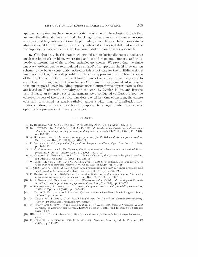
4.3.2. Upper bound through linearization. In order to estimate how con-servative any of the above approximations are compared to the true solution of the(DRSKP-SDP), there is a need for a procedure that might provide an upper boundfor the optimal value of the problem. In order to do so, we exploit the fact that thenonlinearity in constraint (4.4e) is due to the product of two special convex functions.
Lemma 4.8. Function f(y) =√
py
1−py is convex and decreasing for y ∈ ]0, 1] when
p ∈ ]0, 1[. Hence, given any set of values {yl}Ll=1 with each yl ∈ ]0, 1], then we have
f(y) ≥ maxl∈{1,2,...,L}
aly + bl, y ∈ ]0, 1],
where
al =∂(√
py
1−py
)∂y
∣∣∣∣∣∣y=yl
and bl =
√pyl
1− pyl− alyl.
Proof. Since (√
py
1−py )′ = ln p
√py
2(1−py)32≤ 0,when y ∈ ]0, 1], p ∈ ]0, 1[, we have that√
py
1−py is decreasing. Furthermore, since (√
py
1−py )′′ = (ln p)2
4
√py(1+2py)
(1−py)52≥ 0, when
y ∈ ]0, 1], p ∈ ]0, 1[, we confirm that f(y) is convex. Finally, given any yl ∈ ]0, 1],convexity ensures that for all y ∈ ]0, 1],
f(y) ≥ f(yl) + (y − yl)f′(yl)⇒ f(y) ≥ f ′(yl)y + f(yl)− ylf
′(yl)
⇒ f(y) ≥ aly + bl.
This concludes our proof.
Figure 1 provides an illustration of this function for different values of p. Italso illustrates how this function can be lower bounded by a piecewise linear convexfunction which is tangent to the actual function at a finite number of points for anyvalue of p ∈ ]0, 1]. To get an upper bound for the value of our problem, our scheme
0.1 0.2 0.3 0.4 0.5 0.6 0.7 0.8 0.9 10
5
10
15
20
25
30
35
40
45
0 0.1 0.2 0.3 0.4 0.5 0.6 0.7 0.8 0.91
1.5
2
2.5
3
3.5
4
P=0.95
P=0.9
Piecewise linear approximation
Piecewisetangentapproximation
(a) (b)
Fig. 1. Function f(y) =√
py
1−pyis convex and decreasing in y for all p ∈ ]0, 1[. (a) f(y) for
p = 0.5, 0.55, 0.6, 0.7, 0.8, 0.9, 0.95; (b) shows how f(y) can be lower bounded by a piecewise linearconvex function that is tangent to f(y) at a number of points.

1500 JIANQIANG CHENG, ERICK DELAGE, AND ABDEL LISSER
approximates the function√
pyj
1−pyj with a piecewise linear convex lower bounding
function
f(y) = maxl∈{1,2,...,L}
aly + bl ≈√
py
1− py
and linearizes some quadratic terms that emerge after a series of algebraic manipula-tions. We obtain the following upper bounding SDP:
(4.5a)
maximizex,t,q,Q,v,y,z,x
t− μTq− (Σ + μμT ) •Q(4.5b)
subject to
[Q q+akv
2
qT+akvT
2 bk − t
]� 0 ∀ k = {1, 2, . . . ,K},
v(j−1)∗M+i = ARji •X ∀ j ∈ {1, 2, . . . ,M} ∀ i ∈ {1, 2, . . . , n},(4.5c)
Q � 0,(4.5d) ⎡⎣ 0m,m Σ
1/2j Aj
wjTzj
(Σ1/2j Aj
wjTzj)
T 0
⎤⎦(4.5e)
� (μTj Aj
wjTx− djtj)I ∀ j ∈ {1, 2, . . . ,M},(4.5f)
zj ≥ alxj + blx ∀ l ∈ {1, 2, . . . , L} ∀ j ∈ {1, 2, . . . ,M},(4.5g)
M∑j=1
xj = x,(4.5h)
0 ≤ xj ≤ x, (yj − 1)en + x ≤ xj ≤ yjen∀ j ∈ {1, 2, . . . ,M},(4.5i)
M∑j=1
yj = 1, yj ≥ 0 ∀ j ∈ {1, 2, . . . ,M},(4.5j)
[X x
xT 1
]� 0,(4.5k)
Xi,i = xi ∀ i Xi,j ≥ 0 ∀ i, j,(4.5l)
where zj ∈ �n, xj ∈ �n, and en is the vector in �n containing all ones.Theorem 4.9. The optimal value of (4.5) is an upper bound for the optimal
value of (DRSKP-SDP).Proof. The main idea of the proof relies on applying the theory presented in [8].
We focus on the constraint (4.4e). We can first show that{x ∈ �n
∣∣∣∣μTAwj
j x+
√pyj
1− pyj
∥∥∥Σ1/2j Aj
wjTx∥∥∥2≤ dj , j = 1, . . . ,M
}
is equivalent to{x : μTA
wj
j x+
∥∥∥∥Σ1/2j Aj
wjT(√
pyj
1− pyjx
)∥∥∥∥2
≤ dj , j = 1, . . . ,M
}.
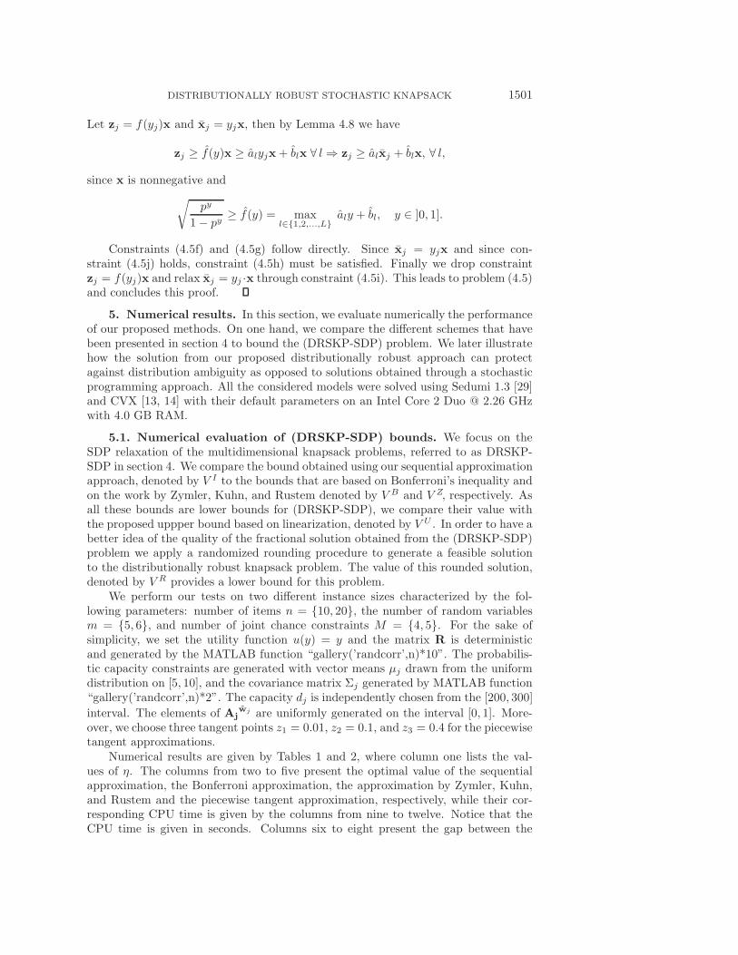
DISTRIBUTIONALLY ROBUST STOCHASTIC KNAPSACK 1501
Let zj = f(yj)x and xj = yjx, then by Lemma 4.8 we have
zj ≥ f(y)x ≥ alyjx+ blx ∀ l⇒ zj ≥ alxj + blx, ∀ l,
since x is nonnegative and√py
1− py≥ f(y) = max
l∈{1,2,...,L}aly + bl, y ∈ ]0, 1].
Constraints (4.5f) and (4.5g) follow directly. Since xj = yjx and since con-straint (4.5j) holds, constraint (4.5h) must be satisfied. Finally we drop constraintzj = f(yj)x and relax xj = yj ·x through constraint (4.5i). This leads to problem (4.5)and concludes this proof.
5. Numerical results. In this section, we evaluate numerically the performanceof our proposed methods. On one hand, we compare the different schemes that havebeen presented in section 4 to bound the (DRSKP-SDP) problem. We later illustratehow the solution from our proposed distributionally robust approach can protectagainst distribution ambiguity as opposed to solutions obtained through a stochasticprogramming approach. All the considered models were solved using Sedumi 1.3 [29]and CVX [13, 14] with their default parameters on an Intel Core 2 Duo @ 2.26 GHzwith 4.0 GB RAM.
5.1. Numerical evaluation of (DRSKP-SDP) bounds. We focus on theSDP relaxation of the multidimensional knapsack problems, referred to as DRSKP-SDP in section 4. We compare the bound obtained using our sequential approximationapproach, denoted by V I to the bounds that are based on Bonferroni’s inequality andon the work by Zymler, Kuhn, and Rustem denoted by V B and V Z, respectively. Asall these bounds are lower bounds for (DRSKP-SDP), we compare their value withthe proposed uppper bound based on linearization, denoted by V U . In order to have abetter idea of the quality of the fractional solution obtained from the (DRSKP-SDP)problem we apply a randomized rounding procedure to generate a feasible solutionto the distributionally robust knapsack problem. The value of this rounded solution,denoted by V R provides a lower bound for this problem.
We perform our tests on two different instance sizes characterized by the fol-lowing parameters: number of items n = {10, 20}, the number of random variablesm = {5, 6}, and number of joint chance constraints M = {4, 5}. For the sake ofsimplicity, we set the utility function u(y) = y and the matrix R is deterministicand generated by the MATLAB function “gallery(’randcorr’,n)*10”. The probabilis-tic capacity constraints are generated with vector means μj drawn from the uniformdistribution on [5, 10], and the covariance matrix Σj generated by MATLAB function“gallery(’randcorr’,n)*2”. The capacity dj is independently chosen from the [200, 300]
interval. The elements of Ajwj are uniformly generated on the interval [0, 1]. More-
over, we choose three tangent points z1 = 0.01, z2 = 0.1, and z3 = 0.4 for the piecewisetangent approximations.
Numerical results are given by Tables 1 and 2, where column one lists the val-ues of η. The columns from two to five present the optimal value of the sequentialapproximation, the Bonferroni approximation, the approximation by Zymler, Kuhn,and Rustem and the piecewise tangent approximation, respectively, while their cor-responding CPU time is given by the columns from nine to twelve. Notice that theCPU time is given in seconds. Columns six to eight present the gap between the
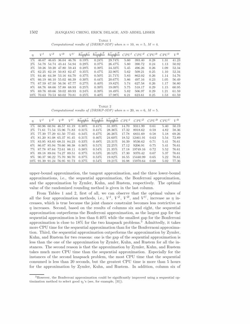
1502 JIANQIANG CHENG, ERICK DELAGE, AND ABDEL LISSER
Table 1
Computational results of (DRSKP-SDP) when n = 10, m = 5, M = 4.
η V I V Z V B V U V U−V I
V IV U−V Z
V ZV U−V B
V B CPUI CPUZ CPUB CPUU V R
1% 46.67 46.65 36.04 46.76 0.19% 0.24% 29.74% 5.60 393.40 0.28 1.31 41.232% 54.78 54.74 43.44 54.94 0.29% 0.37% 26.47% 5.80 390.72 0.24 1.13 50.923% 59.26 59.20 47.80 59.43 0.29% 0.39% 24.33% 5.45 496.26 0.26 1.09 52.344% 62.25 62.18 50.83 62.47 0.35% 0.47% 22.90% 5.62 509.21 0.25 1.10 52.345% 64.46 64.38 53.16 64.70 0.37% 0.50% 21.71% 5.83 862.02 0.26 1.14 54.766% 66.19 66.10 55.02 66.39 0.30% 0.44% 20.67% 5.86 497.16 0.23 1.05 56.497% 67.59 67.50 56.56 67.77 0.27% 0.40% 19.82% 5.74 627.58 0.26 1.17 56.808% 68.76 68.66 57.88 68.93 0.25% 0.39% 19.09% 5.75 518.17 0.29 1.15 60.959% 69.76 69.66 59.02 69.93 0.24% 0.39% 18.49% 5.82 506.97 0.29 1.21 61.5910% 70.63 70.53 60.02 70.81 0.25% 0.40% 17.98% 6.21 623.61 0.25 1.53 61.59
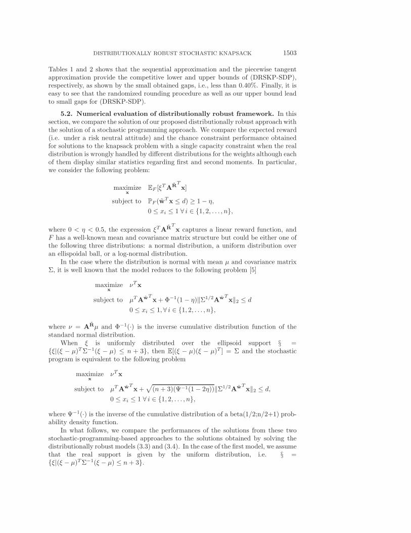
Table 2
Computational results of (DRSKP-SDP) when n = 20, m = 6, M = 5.
η V I V Z V B V U V U−V I
V IV U−V Z
V ZV U−V B
V B CPUI CPUZ CPUB CPUU V R
1% 60.96 60.94 46.57 61.19 0.38% 0.41% 31.39% 14.70 9311.99 0.61 5.40 50.192% 71.61 71.54 55.96 71.83 0.31% 0.41% 28.36% 17.32 8918.62 0.59 4.82 58.363% 77.39 77.29 61.50 77.65 0.34% 0.47% 26.26% 17.78 6831.69 0.58 5.18 69.264% 81.20 81.08 65.37 81.45 0.31% 0.46% 24.60% 18.52 12461.91 0.63 5.54 72.895% 83.95 83.83 68.31 84.23 0.33% 0.48% 23.31% 16.39 9536.62 0.71 5.41 76.616% 86.07 85.94 70.66 86.38 0.36% 0.51% 22.25% 17.12 9206.91 0.75 5.41 76.617% 87.78 87.64 72.61 88.11 0.38% 0.54% 21.35% 17.18 19749.16 0.72 5.52 76.618% 89.18 89.04 74.27 89.51 0.37% 0.53% 20.52% 17.30 9370.42 0.67 5.37 76.619% 90.37 90.22 75.70 90.70 0.37% 0.53% 19.82% 16.55 15440.99 0.65 5.22 76.6110% 91.39 91.24 76.95 91.73 0.37% 0.54% 19.21% 16.98 15970.64 0.68 5.02 77.36
upper-bound approximation, the tangent approximation, and the three lower-boundapproximations, i.e., the sequential approximation, the Bonferroni approximation,and the approximation by Zymler, Kuhn, and Rustem, respectively. The optimalvalue of the randomized rounding method is given in the last column.
From Tables 1 and 2, first of all, we can observe that the optimal values ofall the four approximation methods, i.e., V I , V Z , V B, and V U , increase as η in-creases, which is true because the joint chance constraint becomes less restrictive asη increases. Second, based on the results of columns six and eight, the sequentialapproximation outperforms the Bonferroni approximation, as the largest gap for thesequential approximation is less than 0.40% while the smallest gap for the Bonferroniapproximation is close to 18% for the two knapsack problems.3 Admittedly, it takesmore CPU time for the sequential approximation than for the Bonferrnoni approxima-tion. Third, the sequential approximation outperforms the approximation by Zymler,Kuhn, and Rustem for two reasons: one is the gap of the sequential approximation isless than the one of the approximation by Zymler, Kuhn, and Rustem for all the in-stances. The second reason is that the approximation by Zymler, Kuhn, and Rustemtakes much more CPU time than the sequential approximation. Especially for theinstances of the second knapsack problem, the most CPU time that the sequentialconsumed is less than 20 seconds, but the greatest CPU time is more than 5 hoursfor the approximation by Zymler, Kuhn, and Rustem. In addition, column six of
3However, the Bonferroni approximation could be significantly improved using a sequential op-timization method to select good ηj ’s (see, for example, [31]).
DISTRIBUTIONALLY ROBUST STOCHASTIC KNAPSACK 1503
Tables 1 and 2 shows that the sequential approximation and the piecewise tangentapproximation provide the competitive lower and upper bounds of (DRSKP-SDP),respectively, as shown by the small obtained gaps, i.e., less than 0.40%. Finally, it iseasy to see that the randomized rounding procedure as well as our upper bound leadto small gaps for (DRSKP-SDP).
5.2. Numerical evaluation of distributionally robust framework. In thissection, we compare the solution of our proposed distributionally robust approach withthe solution of a stochastic programming approach. We compare the expected reward(i.e. under a risk neutral attitude) and the chance constraint performance obtainedfor solutions to the knapsack problem with a single capacity constraint when the realdistribution is wrongly handled by different distributions for the weights although eachof them display similar statistics regarding first and second moments. In particular,we consider the following problem:
maximizex
EF [ξTAR
Tx]
subject to PF (wTx ≤ d) ≥ 1− η,
0 ≤ xi ≤ 1 ∀ i ∈ {1, 2, . . . , n},
where 0 < η < 0.5, the expression ξTARTx captures a linear reward function, and
F has a well-known mean and covariance matrix structure but could be either one ofthe following three distributions: a normal distribution, a uniform distribution overan ellispoidal ball, or a log-normal distribution.
In the case where the distribution is normal with mean μ and covariance matrixΣ, it is well known that the model reduces to the following problem [5]
maximizex
νTx
subject to μTAwTx+ Φ−1(1− η)‖Σ1/2AwT
x‖2 ≤ d
0 ≤ xi ≤ 1, ∀ i ∈ {1, 2, . . . , n},
where ν = ARμ and Φ−1(·) is the inverse cumulative distribution function of thestandard normal distribution.
When ξ is uniformly distributed over the ellipsoid support § ={ξ|(ξ − μ)TΣ−1(ξ − μ) ≤ n + 3}, then E[(ξ − μ)(ξ − μ)T ] = Σ and the stochasticprogram is equivalent to the following problem
maximizex
νTx
subject to μTAwTx+
√(n+ 3)(Ψ−1(1− 2η))‖Σ1/2AwT
x‖2 ≤ d,
0 ≤ xi ≤ 1 ∀ i ∈ {1, 2, . . . , n},
where Ψ−1(·) is the inverse of the cumulative distribution of a beta(1/2;n/2+1) prob-ability density function.
In what follows, we compare the performances of the solutions from these twostochastic-programming-based approaches to the solutions obtained by solving thedistributionally robust models (3.3) and (3.4). In the case of the first model, we assumethat the real support is given by the uniform distribution, i.e. § ={ξ|(ξ − μ)TΣ−1(ξ − μ) ≤ n+ 3}.
1504 JIANQIANG CHENG, ERICK DELAGE, AND ABDEL LISSER
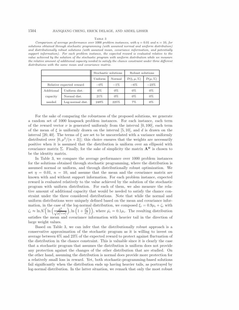
Table 3
Comparison of average performance over 1000 problem instances, with η = 0.01 and n = 10, forsolutions obtained through stochastic programming (with assumed normal and uniform distribution)and distributionally robust solutions (with assumed mean, covariance information, and potentiallysupport information). For each problem instance, the expected reward is evaluated relative to thevalue achieved by the solution of the stochastic program with uniform distribution while we measurethe relative amount of additional capacity needed to satisfy the chance constraint under three differentdistributions with the same mean and covariance matrix.
Stochastic solutions Robust solutions
Uniform Normal D(§, μ,Σ) D(μ,Σ)
Relative expected reward −0% −1% −6% −23%
Additional Uniform dist. 0% 0% 0% 0%
capacity Normal dist. 21% 0% 0% 0%
needed Log-normal dist. 249% 225% 7% 0%
For the sake of comparing the robustness of the proposed solutions, we generatea random set of 1000 knapsack problem instances. For each instance, each termof the reward vector ν is generated uniformly from the interval [0, 100], each termof the mean of ξ is uniformly drawn on the interval [5, 10], and d is drawn on theinterval [20, 40]. The terms of ξ are set to be uncorrelated with a variance uniformlydistributed over [0, μ2/(n + 3)]; this choice ensures that the weights are necessarilypositive when it is assumed that the distribution is uniform over an ellipsoid withcovariance matrix Σ. Finally, for the sake of simplicity the matrix Aw is chosen tobe the identity matrix.
In Table 3, we compare the average performance over 1000 problem instancesfor the solutions obtained through stochastic programming, where the distribution isassumed normal or uniform, and through distributionally robust optimization. Weset η = 0.01, n = 10, and assume that the mean and the covariance matrix areknown with and without support information. For each problem instance, expectedreward is evaluated relatively to the value achieved by the solution of the stochasticprogram with uniform distribution. For each of them, we also measure the rela-tive amount of additional capacity that would be needed to satisfy the chance con-straint under the three considered distributions. Note that while the normal anduniform distributions were uniquely defined based on the mean and covariance infor-mation, in the case of the log-normal distribution, we composed ξi = 0.9μi + ζi with
ζi ≈ lnN(ln(
μ2i√
μ2i+σ2
i
), ln(1 +
σ2i
μ2i
)), where μi = 0.1μi. The resulting distribution
satisfies the mean and covariance information with heavier tail in the direction oflarge weight values.
Based on Table 3, we can infer that the distributionally robust approach is aconservative approximation of the stochastic program as it is willing to invest onaverage between 6% and 23% of the expected reward to protect against fluctuation ofthe distribution in the chance constraint. This is valuable since it is clearly the casethat a stochastic program that assumes the distribution is uniform does not provideany protection against the changes of the other distribution that are studied. Onthe other hand, assuming the distribution is normal does provide more protection fora relatively small loss in reward. Yet, both stochastic-programming-based solutionsfail significantly when the distribution ends up having heavier tails, as portrayed bylog-normal distribution. In the latter situation, we remark that only the most robust
DISTRIBUTIONALLY ROBUST STOCHASTIC KNAPSACK 1505
approach still preserves the chance constraint requirement. The robust approach thatassumes the ellipsoidal support might be thought of as a good compromise betweenstochastic and fully robust solutions. In particular, we see that the chance constraint isalways satisfied for both uniform (as theory indicates) and normal distribution, whilethe capacity increase needed for the log-normal distribution appears reasonable.
6. Conclusions. In this paper, we studied a distributionally robust stochasticquadratic knapsack problem, where first and second moments, support, and inde-pendence information of the random variables are known. We prove that the singleknapsack problem can be reformulated as an SDP after applying the SDP relaxationscheme to the binary constraints. Although this is not case for the multidimensionalknapsack problem, it is still possible to efficiently approximate the relaxed versionof the problem and obtain upper and lower bounds that appear numerically close toeach other for a range of problem instances. Our numerical experiments also indicatethat our proposed lower bounding approximation outperforms approximations thatare based on Bonferroni’s inequality and the work by Zymler, Kuhn, and Rustem[34]. Finally, an extensive set of experiments were conducted to illustrate how theconservativeness of the robust solutions does pay off in terms of ensuring the chanceconstraint is satisfied (or nearly satisfied) under a wide range of distribution fluc-tuations. Moreover, our approach can be applied to a large number of stochasticoptimization problems with binary variables.
REFERENCES
[1] D. Bertsimas and M. Sim, The price of robustness, Oper. Res., 52 (2004), pp. 35–53.[2] D. Bertsimas, K. Natarajan, and C.-P. Teo, Probabilistic combinatorial optimization:
Moments, semidefinite programming and asymptotic bounds, SIAM J. Optim., 15 (2004),pp. 185–209.
[3] A. Billionnet and F. Calmels, Linear programming for the 0-1 quadratic knapsack problem,Eur. J. Oper. Res., 92 (1996), pp. 310–325.
[4] P. Brucker, An O(n) algorithm for quadratic knapsack problems, Oper. Res. Lett., 3 (1984),pp. 163–166.
[5] G. C. Calafiore and L. El Ghaoui, On distributionally robust chance-constrained linearprograms, J. Optim. Theory Appl., 130 (2006), pp. 1–22.
[6] A. Caprara, D. Pisinger, and P. Toth, Exact solution of the quadratic knapsack problem,INFORMS J. Comput., 11 (1999), pp. 125–137.
[7] W. Chen, M. Sim, J. Sun, and C. P. Teo, From CVaR to uncertainty set: implications injoint chance constrained optimization, Oper. Res., 58 (2010), pp. 470–485.
[8] J. Cheng and A. Lisser, A second-order cone programming approach for linear programs withjoint probabilistic constraints, Oper. Res. Lett., 40 (2012), pp. 325–328.
[9] E. Delage and Y. Ye, Distributionally robust optimization under moment uncertainty withapplication to data-driven problems, Oper. Res., 58 (2010), pp. 596–612.
[10] L. El Ghaoui, M. Oks, and F. Oustry, Worst-case value-at-risk and robust portfolio opti-mization: a conic programming approach, Oper. Res., 51 (2003), pp. 543–556.
[11] A. Gaivoronski, A. Lisser, and R. Lopez, Knapsack problem with probability constraints,J. Global Optim., 49 (2011), pp. 397–413.
[12] G. Gallo, P. Hammer, and B. Simeone, Quadratic knapsack problems, Math. Program. Stud.,12 (1980), pp. 132–149.
[13] M. Grant and S. Boyd, CVX: MATLAB Software for Disciplined Convex Programming,Version 2.0 Beta http://cvxr.com/cvx (2012).
[14] M. Grant and S. Boyd, Graph Implementations for Nonsmooth Convex Programs, RecentAdvances in Learning and Control, Lecture Notes in Control and Inform. Sci., Springer:Berlin, 2008.
[15] IBM ILOG, CPLEX Optimizer, http://www.ibm.com/software/integration/optimization/cplex/.
[16] E. Johnson, A. Mehrotra, and G. Nemhauser, Min-cut clustering, Math. Program., 62(1993), pp. 133–152.
1506 JIANQIANG CHENG, ERICK DELAGE, AND ABDEL LISSER
[17] P. Kouvelis and G. Yu, Robust Discrete Optimization and its Application, Kluwer Academic,Dordrecht, 1997.
[18] H. Kellerer, U. Pferschy, and D. Pisinger, Knapsack Problems, Springer, Berlin, 2004.[19] S. Kosuch and A. Lisser, Upper bounds for the stochastic knapsack problem and a B&B
algorithm, Ann. Oper. Res., 176 (2010), pp. 77–93.[20] S. Kosuch and A. Lisser, On two-stage stochastic knapsack problems with or without proba-
bility constraint, Discrete Appl. Math., 159 (2011), pp. 1827–1841.[21] M. Kress, M. Penn, and M. Polukarov, The minmax multidimensional knapsack prob-
lem with application to a chance-constrained problem, Naval. Res. Logist., 54 (2007),pp. 656–666.
[22] S. Liao, C. van Delft, and J. P. Vial, Distributionally robust workforce scheduling in callcenters with uncertain arrival rates, Optim. Methods Softw., 28 (2013), pp. 501–522.
[23] A. Lisser and R. Lopez, Stochastic quadratic knapsack with recourse, Electron. Notes DiscreteMath., 36 (2010), pp. 97–104.
[24] S. Martello and P. Toth, Knapsack Problems: Algorithms and Computer Implementations,John Wiley, New York, 1990.
[25] M. Monaci and U. Pferschy, On the robust knapsack problem, SIAM J. Optim., 23 (2013),pp. 1956–1982.
[26] I. Polik and T. Terlaky, A survey of the S-Lemma, SIAM Rev., 49 (2007), pp. 371–418.[27] H. Scarf, A min-max solution of an inventory problem, in Studies in the Mathematical Theory
of Inventory and Production, Stanford University Press, Stanford, CA, 1958, pp. 201–209.[28] A. Shapiro, On the duality theory of conic linear problems, in Semi-Infinite Programming:
Recent Advances, Kluwer Academic, Dordrecht, 2001, pp. 135–165.[29] J. F. Sturm, Using SeDuMi 1.02, a Matlab toolbox for optimization over symmetric cones,
Optim. Method. Softw., 11–12 (1999), pp. 625–653.[30] M. R. Wagner, Stochastic 0–1 linear programming under limited distributional information,
Oper. Res. Lett., 36 (2008), pp. 150–156.[31] W. Wiesemann, D. Kuhn, and B. Rustem, Multi-resource allocation in stochastic project
scheduling, Ann. Oper. Res., 193 (2012), pp. 193–220.[32] W. Wiesemann, D. Kuhn, and M. Sim, Distributionally robust convex optimization, Oper.
Res., to appear.[33] K. Yoda and A. Prekopa, Convexity and Solutions of Stochastic Multidimensional Knapsack
Problems with Probabilistic Constraints, Technical report Rutgers Center for OperationsResearch, New Brunswick, NJ, 2012.
[34] S. Zymler, D. Kuhn, and M. Rustem, Distributionally robust joint chance constraints withsecond-order moment information, Math. Program., 137 (2013), pp. 167–198.