DISUSSIN PAP SIS - ftp.iza.orgftp.iza.org/dp11726.pdf · method as Saiz and Wachter (2011) using the UK labor force survey. She concludes that a 1 She concludes that a 1 percent increase

DISCUSSION PAPER SERIES

IZA DP No. 11726

Josef KjellanderViktor NilssonAico van Vuuren

The Impact of the Announcement of Temporary Building Sites for Refugees on House Prices in Gothenburg

AUGUST 2018

Any opinions expressed in this paper are those of the author(s) and not those of IZA. Research published in this series may include views on policy, but IZA takes no institutional policy positions. The IZA research network is committed to the IZA Guiding Principles of Research Integrity.The IZA Institute of Labor Economics is an independent economic research institute that conducts research in labor economics and offers evidence-based policy advice on labor market issues. Supported by the Deutsche Post Foundation, IZA runs the world’s largest network of economists, whose research aims to provide answers to the global labor market challenges of our time. Our key objective is to build bridges between academic research, policymakers and society.IZA Discussion Papers often represent preliminary work and are circulated to encourage discussion. Citation of such a paper should account for its provisional character. A revised version may be available directly from the author.

Schaumburg-Lippe-Straße 5–953113 Bonn, Germany

Phone: +49-228-3894-0Email: [email protected] www.iza.org

IZA – Institute of Labor Economics

DISCUSSION PAPER SERIES

IZA DP No. 11726

The Impact of the Announcement of Temporary Building Sites for Refugees on House Prices in Gothenburg

AUGUST 2018

Josef KjellanderUniversity of Gothenburg

Viktor NilssonUniversity of Gothenburg

Aico van VuurenUniversity of Gothenburg, Georgetown Center for Economic Research and IZA

ABSTRACT

IZA DP No. 11726 AUGUST 2018

The Impact of the Announcement of Temporary Building Sites for Refugees on House Prices in Gothenburg*

We evaluate the price development of apartments in neighborhoods surrounding temporary

housing for refugees using the unpredicted announcement of three building sites, targeting

refugees, in Gothenburg. More in particular, we look at the price development in the year

after the announcement. We use a causal outcome model that takes account of time and

postal-code fixed effects and we define an area to be affected by the announcement based

on walking distance. We find support for a small and significant price effect. In addition,

we find that the price effect of the neighborhood depends on the income level of the

neighborhood. We interpret this as evidence for the fact that not having to live close to

refugees can be seen as a luxury good.

JEL Classification: O15, O18, R31

Keywords: house prices, migration

Corresponding author:Aico van VuurenDepartment of EconomicsUniversity of GothenburgVasagatan 1SE-405 30 GothenburgSweden

E-mail: [email protected]

* We would like to thank Stuart Rosenthal for his useful comments.

1 Introduction

Investments in property as dwellings are often the largest financial decisions for individuals

during their lifetime. Therefore, stability and predictability of the housing market in terms

of price and price developments are desirable and governmental policy should target such

predictability. Nevertheless, governments often need to make decisions that can have un-

predicted and negative impacts on the price development in some neighborhoods. One such

decision is the construction of refugee housing and therefore, this has been used as an argu-

ment when opposing specific (temporary) housing sites for refugees 1. Despite its importance,

there are hardly any papers investigating the impact of refugee housing on neighboring house

prices (Lastrapes and Lebesmuehlbacher, 2017, constitute an exception). This knowledge

gap creates a great difficulty in addressing the question of where and whether to build refugee

housing. Therefore, we examine the recent events in Gothenburg, where the construction of

twelve temporary housing sites was announced in January 2016 and investigate its impact

on house prices.

For this purpose, we collect data on property sales within Gothenburg between 2014 -

2017 and generate a distance variable with a unique value for every property by extracting

information on coordinates from geo-coded data. Similar to previous research on the housing

market, this paper builds on the hedonic pricing method, which assumes that the price of a

good is determined by both internal (such as the number of rooms and living area) as well

as external factors (such as neighborhood factors). Due to the attention (pattern) that the

announcement attracted, we argue that the locations were not anticipated and treat it as a

natural experiment. We estimate an empirical model with time and region fixed effects to

examine if the price per square meter trend has been different for the properties surrounding

1See Goteborgs Posten, “SD mobiliserar mot flyktingboenden: “Folk ar radda”“, February, 4th, 2016.

1

the announced locations after the announcement, as compared to the trend in the rest of

Gothenburg. Our objective is to investigate whether the announcement can have any impact

rather than to find out by exactly how much the house prices changed for individual houses.

The latter is a much more difficult question to answer because of general equilibrium effects

and the sensitivity to the exact specification of the econometric model.

In our analysis, we focus on the price per square meter for apartments. This is a relatively

liquid and homogeneous asset and we would like to separate it from single family houses.

The reason for this separation is also due to the special regulations regarding the ownership

of apartments in Sweden (Hjalmarsson and Hjalmarsson, 2009). Our results indicate that

there has been a negative effect on surrounding apartment prices. More in particular, we

find that houses that were sold in the year after the announcement and that were within a

15-minute walking distance were sold at a price that was around 3 percent lower than the

houses that were sold at a longer distance from temporary housing for refugees. We perform

a number of robustness checks such as changing the cutoff value of a 15-minute walk to a

10- and 20-minute walk, respectively, changing the comparison group and we delete some

outliers in terms of price. Although the robustness checks indicate that some of our results

may have been driven by the extremely cheap and expensive houses, we find an overall,

robust and negative impact of the temporary building sites. We interpret this as a new

result, especially since the refugee housing was not even built in the period of our analysis.

Even though the number of papers that have been looking at refugee housing is far from

abundant, there is ample research on the impact of the inflow of immigrants on house prices.

Using US data, Saiz (2007) finds that there was a larger appreciation of house prices in

areas where immigrants more frequently settled between 1983 and 1997 due to an increased

demand. Saiz and Wachter (2011) use decennial data for US metropolitan areas at the census

2

tract level (small areas with on average 4000 inhabitants) to evaluate if having immigrant

neighbors affects house prices. They find that the appreciation of house prices is negatively

affected by the growth of a neighborhood’s immigrant share. Sa (2015) adopts a similar

method as Saiz and Wachter (2011) using the UK labor force survey. She concludes that a 1

percent increase in the stock of immigrants results in a 1.7 percent decrease in house prices.

She also finds that this impact is driven by a negative impact in the poorest neighborhoods

(with the lowest levels of education), while the negative impact is shown to mainly be driven

by the fact that the highest earning families in the poor neighborhoods move after an increase

in the immigrant population. One problem of all mentioned research is that immigration

in general has two opposing impacts. First, immigration has a positive impact on housing

demand, which is driven directly by the immigrants. Second, due to the potential outflow of

families, there is a negative impact on housing demand. These two opposing impacts make

the total impact ambiguous and the results somewhat hard to interpret. We do not have this

problem in our analysis, since the building sites do not directly compete with the existing

housing supply.

The only paper that studies the impact of refugees on house prices is from Lastrapes

and Lebesmuehlbacher (2017). They mention that refugees are demographically different

from many other types of immigrants (especially in terms of education). Moreover, refugees

typically do not make their choice of residence based on the economic situation of the neigh-

borhood and, in many cases, do not have any say at all in their location decision. Lastrapes

and Lebesmuehlbacher (2017) find that there is an ambiguous impact of refugees on house

prices in general. However, they find an unambiguously small and negative impact for low-

priced houses and houses of low quality. One challenge in their research is that refugees

are typically located in hard-to-let residential housing, which is usually located in neighbor-

3

hoods that are not doing well in the first place. They correct for this problem by using an

instrument (i.e. the change in the share of subsistence-only asylum seekers located in neigh-

boring districts). We do not have this problem in our analysis since the chosen locations

in Gothenburg were selected based on the objective to omit segregation and are therefore

randomly chosen by the municipality.

Gautier, Siegmann and van Vuuren (2009) is closely related to our paper in terms of

research question and empirical strategy. They investigate whether the assassination of the

controversial movie maker Theo van Gogh in Amsterdam in 2004, carried out by a radical

Muslim, affected house prices differently in these neighborhoods. Using a difference-in-

difference approach, the authors discover that after the murder, house prices in neighbor-

hoods with a relatively large number of migrants from a Muslim country experienced around

a 0,07% lower increase per week.

In the final part of the paper, we try to explain our results. Since the housing sites form

a different market than the present housing stock, supply changes are not likely to explain

these results. Hence, we expect them to be largely driven by demand changes of potential

buyers in the affected areas. As potential explanations, we investigate immigrants density,

education and income levels. We find that difference in income forms the most import

determinant for the severity of the price decrease. That is, low income neighborhoods do not

seem to suffer any price loss. Hence, we interpret our results as evidence for the fact that

not having to live close to refugees can be seen as a luxury good which becomes important

for higher income levels. We also find that neither education nor the number of immigrants

has a large impact on the results.

The paper has the following outline. We present a background to the events in 2015

and 2016 in Section 2. Section 3 describes the data and the key variables of interest and

4

is followed by our empirical strategy in Section 4. The results are presented in Section 5

and we investigate the robustness of the results in Section 6. Section 7 discusses potential

explanations of our results. Section 8 presents our conclusions.

2 Background

Due to the war in Syria and an increased migration from northern Africa, the inflow of

migrants to Sweden increased rapidly during the second half of 2015. At its peak in November

2015, Sweden received around 10,000 applications for asylum each week, as compared to

around 2,000 per week in 2014. By the end of 2015, 162,877 people had been seeking asylum

in Sweden - as compared to 81,301 in 2014 and 54,259 in 2013. This increase put a great

deal of pressure on the Swedish reception system and led to problems providing housing for

the new residents.

The Swedish housing market in the major cities was affected by the large inflow of

refugees, but the market had already been struggling for some time before 2015, thus creating

a large deficit of housing.2 An estimated 700,000 new homes need to have been built by 2025

to cover this deficit. Further, there are pronounced insider-outsider effects in the Swedish

housing market.3 In the fall of 2015, the city of Gothenburg announced that it was to build

1000 apartments on temporary building permits targeting the newly arrived in order to

address some of the more acute issues.

Locations for twelve temporary housing sites were presented on January 28th, 2016. Since

the day of the announcement, there has been a substantial newspaper coverage on the issue.

As an illustration, Figure 1 shows the newspaper coverage in one of the most important

2For example, the average waiting time for a rental apartment has increased from about 2 to 4 years inthe period 2012 - 2016 .

3See for example an article published in the Gaurdian by D. Crouch, “Pitfalls of rent restraints: whyStockholm’s model has failed many ”, August, 19th, 2015.

5

newspapers in the city of Gothenburg using the Google search words temporary, houses and

refugees. The locations were chosen considering certain characteristics such as communica-

tion, service and a low share of refugees in that particular city area, the last one in order

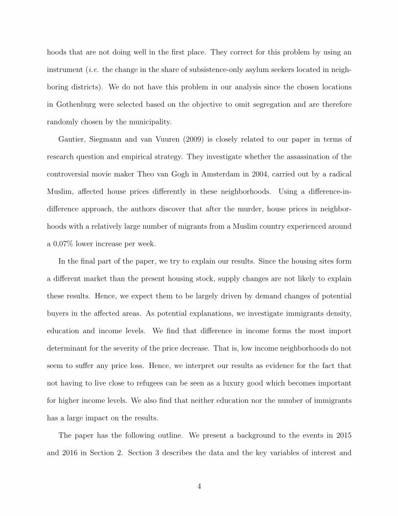
to combat segregation (Goteborgs stad, 2016). Figures 3 and 4 show the locations of the

temporary building sites. Since the announcement, all sites have been debated and further

evaluated. At the end of May 2017, the temporary building permit was approved for three

sites (Karralundsvallen and Askimsbadet and Lemmingsvallen). The remainder of the sug-

gested locations have been rejected for various reasons. A timeline summarizing the events

for all of the sites can be seen in Figure 2. Therefore, we only use these three building sites

for our analysis. The number of apartments currently planned to be built on these three

sites were 158. 44 out of these were planned at Karralundsvallen and 114 were planned

(with an equal split) at Askimsbadet and Lemmingsvallen. At the end of September 2017,

Karralundsvallen and Lemmingsvallen decided to no longer use their building permit due to

the high costs involved. However, this date is quite far from our observation window.

3 Data

We collected data for around 20,000 properties from the site Booli.se (using their API to

retrieve it). Booli is an independent search engine for private properties. The site collects

publicly available data from most real-estate agencies’ websites. One does not need to

actively advertise on Booli for the property to be available on the website; it only needs to

be available on the real-estate agencies’ websites. Apart from the houses that are currently

for sale, Booli also presents houses that have been sold since 2012 and this is the information

that we use for our analysis. This data only includes sales made by open ascending bids

(the most common way of selling a property in Sweden). All sales that took place before the

6

−200−100 0 100 200 300 400 500

0

1

2

3

4

5

6

Days after the announcement

New

spap

erar

ticl

es

Figure 1: Number of newspaper articles published per week in Goteborgs Posten from 6 monthsbefore the announcement to one year after the announcement.

1/1 28/1

Ann

ounc

emen

tof

the12

pote

ntial

site

s

7/3

Hin

sholm

en, A

mun

don,

Skin

tebo

smab

atsh

amn,

Tuvean

dFis

keba

ck

reject

ed

17/5

Ana

sfalte

tre

ject

ed

19/8

Bui

ldin

gpe

rmit

sent

info

r

Ask

imsv

iken

11/10

Bui

ldin

gpe

rmit

sent

info

r

Kar

ralu

ndsv

allen

and

Lemm

ings

valle

n

25/10

Bui

ldin

gpe

rmit

appr

oved

for

Ask

imsv

iken

3/11

Bjo

rkek

arrspl

an, G

lasm

asta

rega

tan

and

Frid

kulla

gata

nre

ject

ed

20/12

Bui

ldin

gpe

rmit

appr

oved

for

Kar

ralu

ndsv

allen

Figure 2: Timeline of events in 2016 (time-scale not proportional)

7

start of the bidding process are not public and hence not available through their API.

We use the open source routing machine (OSRM) to calculate the walking distances

between the apartments and the temporary building sites. Using walking distances instead

of using physical (Euclidean) distances has the advantage of accounting for the fact that there

are many rivers, islands, forests and hills in Gothenburg and hence even though two sites

might be very close to each other based on geographic location, the distance to move between

these locations may take quite some time. Since we use rather short walking distances, i.e.

15 minutes for our baseline analysis, it can be expected that our choice does not depend to

any great extent on the mode of transport. That is, the ranking between two locations is

unlikely to be affected by this mode of transport. The reason for using walking distance is

that we do not want our results to be affected by the fact that some houses are located very

close to either a major railway station or a highway and are therefore closely related to a

huge range of different locations including the temporary building sites.

In terms of geographical area, our data set covers the municipality where the sites are

located (Gothenburg) and to which they border (Molndal and Partille), while the time period

in our most general specification is January 2014 - November 2017.4 This means that the

data consists of two years prior to the announcement of the temporary housing sites until

almost two years after the announcement. However, since we typically look at the impact

up to one year after the announcement, our baseline time window is from January 2014

to January 2017. A relatively short time period in our baseline analysis has been chosen

to reduce the probability of things other than the treatment affecting the property prices.

Further, both data sets have been cleaned from obvious misreports, missing values and

properties not suitable for year-round living.5

4Molndal and Partille are included since at least one of the original twelve sites are within 1 kilometerof the municipality border.

5Properties not suitable for year-round living include summer houses and houses that only have running

8

A few notes should be made about the data set and the Swedish market. First, apartment

buyers do not really own the property in Sweden. Instead, they acquire shares (or rights) of

an economic association that owns the property. This is always the case for apartments, but

also smaller houses (which are typical within Gothenburg) have this arrangement. The buyer

of the shares obtains the right as a single user of the property, but she also has to pay a rent

for using it. This arrangement is also common in other Nordic countries, but not elsewhere.

Note that the rents are substantial and vary a great deal between the different properties

(Hjalmarsson and Hjalmarsson, 2009). Hence, we cannot simply compare owned houses

with houses that have these arrangements. This is the reason why we focus on apartments

rather than on owned houses in our analysis. It implies that the total number of properties

available for us is around 13,500. Second, selling prices are collected from Booli’s website as

the last/highest bids. For most cases, this will correspond to the selling price and in those

cases that it does not, it still serves as a good valuation of the property. There are two

scenarios when the highest bid does not correspond to the selling price: (1) the seller sells

to a lower bidder or does not sell at all and (2) the highest bidder withdraws her bid. Both

reasons are not necessarily problematic in our analysis as long as the valuation derived from

the highest bid is still consistent with the market valuation in the hedonic pricing model to be

discussed in the next section. Third, the market for properties was booming in Gothenburg

during our observation window. There is a deficit of properties and the average time that

an object is for sale is short. It is not unusual that objects are sold before the start of the

bidding process.6 As previously mentioned, these sales are not included in our data set. This

can potentially underestimate the (absolute value of the) impact of the temporary building

sites if less houses are sold before the bidding starts in the areas close to these sites during

water and electricity half of the year.6According to the site Hemnet, 25% of all properties in Gothenburg were sold before the bidding began

in 2016.

9

the period of our analysis. That is, some extremely good houses in these areas would not

have been observed in our data set in the case that the building sites were not announced,

because they would have been sold before the bidding starts.

As an alternative, we could have used the Swedish register for property in our analysis.

However, apart from the fact that it will result in fewer control variables, this has two

drawbacks. First, the majority of houses within the city of Gothenburg are apartments and

these are not registered by the Swedish register. Second, the register only uses the date of the

change of ownership, which is typically a couple of months after the date of the transaction.

Booli uses the date at which the final offer was made and this is a more accurate date for

our analysis than the date of changing ownership.

The descriptive statistics for the dependent variable, price per square meter, and the

control variables are listed in Table 1. Control variables in the regressions consist of living

area, construction year, square meters per room, yearly rent per square meter and floor. The

descriptive statistics are split up between apartments situated at either within or outside

the affected areas of the three sites that are still considered in May 2017 (Askimsbadet,

Karralundsvallen and Lemmingsvallen). From this point, only these three sites are included

in our analysis if nothing else is mentioned.

We define whether a house is within the affected area by using walking distance to any of

the temporary building sites. In our baseline analysis, we use a 15-minute walking distance.

We expect that this distance is close enough to potentially be directly affected by the sites

as well as indirectly affected by the rumors going around about how the sites will affect

neighborhoods. As can be seen in Table 1, there are 495 apartments in the “affected” area

that were sold during our time window. 150 of these were sold during the year after the

announcement. We also consider other cut-off distances to investigate if this changes the

10

Table 1: Descriptive Statistics

Apartments Apartmentswithin outside

mean sd mean sd

Price 2874.18 1093.98 2725.35 1268.20Price/m2 47.22 10.65 43.10 14.92Living area (m2) 61.91 21.13 65.43 22.98Construction year 1951.62 23.25 1957.58 31.43Rooms 2.37 0.96 2.43 0.93m2/rooms 27.48 5.69 28.00 5.58Rent 3410.08 1022.73 3667.86 1151.63Yearly rent/m2 683.92 142.11 690.91 129.75Floor 2.08 0.92 2.73 1.86Number of observations 495 12907

results. With a cut-off distance of 10 minutes, the number of observations within the affected

area is 224 apartments (of which 65 were in the year after the announcement), while a 20

minute walking distance results in an affected group of 1073 apartments (of which 341 were

in the year after the announcement).

Apartments in the affected areas are, on average, somewhat more expensive, especially

when we look at the price per square meter. Remember that the aim was to build the tem-

porary building sites in areas with good communications and services and thus not increase

the segregation. It is therefore not surprising that properties in areas surrounding these sites

on average have higher prices per square meter, compared to the rest of Gothenburg.

Apartments located outside the threshold distance are, on average, roughly 10% larger -

resulting in the relationship previously mentioned concerning price and square meter price.

There is also roughly a 10% difference in monthly rent, but it is also found that this difference

can be completely ascribed to the difference in size; the rent per square meter is virtually

identical for the two types of areas. Therefore, we use yearly rent per square meter as the

control variable for our regressions. We do the same for the number of rooms that we alter

11

to square meters per room.7

We use the logarithm for the variables price per square meter, living area, square meter

per room and yearly rent per square meter. This has the advantage that the relative difference

in these variables is a better measurement than the absolute difference and also typically

reduces heteroskedasticity (improving efficiency).

The total number of months in the data is 38 for both houses and apartments. 26 out of

these are before the announcement and 12 are after. Postal codes will be included to control

for external characteristics. For our baseline analysis, the dataset consists of 358 unique

postal codes. Months and postal codes will be included as dummies in the empirical model

in order to control for time and neighborhood fixed effects.

4 Empirical strategy

We use the following baseline model:

logPijt = β0 + δ1Dwithini + δ2D

withini ∗Dpost

t + β′3Xi + αj + λt + Uijt, (4.1)

where i indicates individual property, j indicates neighborhood and t indicates time. logPijt

is our outcome variable and is defined as the log price per square meter. The variable

Dwithini is a dummy indicating if a property is within the threshold (walking) distance to

any of the temporary housing sites (i.e. within a 15-minute walking distance in our baseline

model). Dpostt is a time dummy equal to 1 after the sites were announced and zero before.

The interaction term between the two dummies Dpostt ∗ Dwithin

i is the variable of interest:

it measures the mean impact of the price per square meter for houses within the threshold

7The alternation of the variables does not change the outcome in terms of significance. It only changesthe parameter value and the fit of the model marginally, as compared to when including them in their originalform.

12

distance after the announcement, as compared to houses outside the threshold distance,

keeping everything else constant. We can interpret this impact as causal as long as Uijt is

independent from the regressors (including the fixed effects). Here, a causal impact implies

that we can interpret it as the impact due to the announcement of the temporary building

sites, i.e. the average observed houseprice minus the houseprice that we would have observed

had there been no announcement.

In order to make the assumption of independence between Uijt and Dwithini and Dwithin

i ∗

Dpostt more plausible, a vector of house characteristics (Xi) is included as well as time (λt)

and neighborhood (αj) fixed effects. A key assumption is that the announcement - the

treatment effect - can be considered as an exogenous and not anticipated event. As was

already shown in Figure 1, the announcement of the twelve original sites received much

attention by the public and media and we argue that this strengthens the assumption that

they were unanticipated.

Our approach focuses on the investigation of whether there is any impact of the announce-

ment of the temporary building sites on the price of the houses close to those building sites.

We do not aim at estimating the exact impact or explaining such an impact based on dis-

tance or type of area or house. Hence, even though specification (4.1) may be restrictive, it

suffices for our research question. For example, it may be possible that instead of (4.1), the

actual relationship is as follows:

logPijt = β0 + δ2f(Di)Dpostt + β′

3Xi + αj + λt + Uijt,

where Di is the distance to any of the temporary building sites and f is a decreasing function

of this distance. Naturally, it may be interesting to estimate the function f , but it is clear

that if f decreases sufficiently around the cut-off value, then our parameter of interest, i.e.

13

δ2 in (4.1), should be negative. Moreover, it is impossible to have a negative sign of δ2

even in the case that f is completely flat for any value of Di. Still, in order to obtain more

confidence in our results, we do investigate whether our results are affected by changes in

the cut-off value.

As stated above, our approach yields the possibility to obtain a causal treatment effect.

However, there are some crucial assumptions for this approach to be applicable: (1) there

must be a parallel trend before the announcement between the affected group and the re-

maining houses in order to justify the assumption that the trend would have been equal in

the case of no treatment, (2) the method assumes that the unobserved characteristics before

and after treatment are equal. This means that properties sold within the areas of interest

have similar unobserved characteristics before and after the treatment. If this is not the

case, for example, if the supply of properties in terms of their attractiveness is more skewed

to the right after the treatment relative to before, a negative treatment effect could appear

due to the fact that less expensive properties are bought at that time (an indirect treatment

effect), (3) there cannot be any spillover effect from the affected to the non-affected areas.

Although properties cannot be moved, this problem may arise due to general equilibrium

effects, i.e. the fact that some areas become less attractive may increase the prices in other

areas. Although this can have an impact on the precise value of our estimate, it will not

affect the sign.

Since the model controls for time and neighborhood fixed effects, it controls for variables

that differ across the different geographic areas but are constant over time (such as proximity

to the ocean) and for variables that evolve over time, but are the same for all geographical

areas (such as interest rate). Time fixed effects consist of monthly time dummy variables

and neighborhood fixed effects are dummy variables for postal code.

14

5 Results

Table 2 lists the main results of this paper. The variable within “walking distance” implies

that one of the three building sites is within a 15-minute walking distance from the apartment

that is sold. The impact of the announcement of the building sites is measured by the

variable that indicates that the house is within walking distance and sold after the date

of the announcement. In our baseline analysis, we correct for a full set of dummy postal

codes and hence the impact of the announcement of the building sites is identified from the

fact that there are houses within a postal code that can either be shorter or longer than

a 15-minute walk to the building site. We find that houses within this walking distance

from the temporary building sites had a 3.3 percent lower increase in their house prices than

houses situated further from those building sites. Based on the use of heteroskedasticity

robust standard errors, as we do in the first column of Table 2, we can conclude that the

impact is also significant. As a robustness check, we also provided the standard errors based

on clustering of the postal codes. Note that the use of such clustered standard errors is

only correct in the case that there is substantial heterogeneity in terms of the impact of the

building sites between the postal codes (see Abadie, Athey and Wooldridge, 2017). If this

is not the case, then these clustered standard errors are biased. In fact, the impact of the

building sites is modeled to be homogeneous, i.e. specification (2), which makes the use

of the standard heteroskedasticity robust standard errors more appropriate. Nevertheless,

given the fact that we use three different building sites, which implies that the postal codes

that are affected can be quite far from each other, it is possible that there is heterogeneity.

As can be seen from the second column of Table 2, the clustered standard error of the impact

is somewhat higher than the heteroskedasticity robust standard error, but the impact is still

15

significantly different from zero (based on a significance level of 5 percent).8

Note that our model is identified since there are postal code areas that have both affected

and not affected houses, i.e. areas for which the cutoff line of a 15-minute walk crosses

the postal code area. Both the use of a 15-minute walk and the use of the lowest level

of aggregation of the postal codes are arbitrary. The assumption of a 15-minute walk is

discussed in the next section. Here we discuss the use of the aggregation of postal codes.

The third column of Table 2 lists our results in the case that we use only the first four digits

of the postal code area. Surprisingly, our results are not affected to any extent by using such

a level of aggregation although the standard error of the impact of the temporary building

sites is slightly higher. When we use an even higher level of aggregation, then we are no

longer able to say anything about the impact and the impact is quantitatively close to zero.

However, it is questionable whether this is the right level of aggregation since it implies that

many houses within a postal code can be quite different from each other. Remember that

the temporary building sites are very good areas in Gothenburg and using a high level of

aggregation implies that we compare very good areas that are within this long “walking

distance” from the temporary building sites to lower ranked areas that are not close to the

temporary building sites. This is exactly what happens when going from columns 1 and 2

to columns 3 and 4 of Table 2 when we look at the within walking distance dummy variable:

it grows from virtually equal to zero to around 7 percent.

In order to investigate whether the temporary building sites had the same price develop-

ment as the non-affected areas, we report the results of an extension of the model reported

in columns 1 and 2 of Table 2 in column 5 of that table, where we also include an interaction

dummy of the affected areas with the year 2015. This is to investigate whether our results

8Note that the use of a more aggregate level of clustering would have been an error in this case. That is,the heterogeneity should be expected at the same level as the level used for the postal code dummy variables.

16

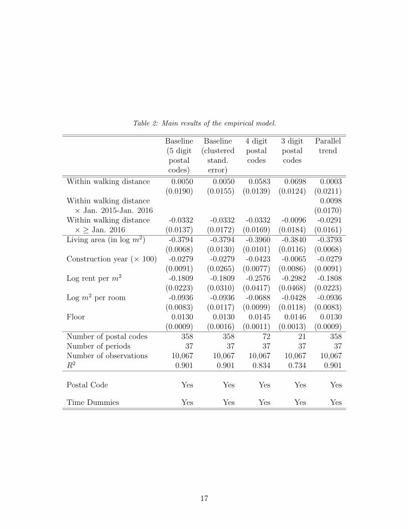
Table 2: Main results of the empirical model.

Baseline Baseline 4 digit 3 digit Parallel(5 digit (clustered postal postal trendpostal stand. codes codescodes) error)

Within walking distance 0.0050 0.0050 0.0583 0.0698 0.0003(0.0190) (0.0155) (0.0139) (0.0124) (0.0211)

Within walking distance 0.0098× Jan. 2015-Jan. 2016 (0.0170)

Within walking distance -0.0332 -0.0332 -0.0332 -0.0096 -0.0291× ≥ Jan. 2016 (0.0137) (0.0172) (0.0169) (0.0184) (0.0161)

Living area (in log m2) -0.3794 -0.3794 -0.3960 -0.3840 -0.3793(0.0068) (0.0130) (0.0101) (0.0116) (0.0068)

Construction year (× 100) -0.0279 -0.0279 -0.0423 -0.0065 -0.0279(0.0091) (0.0265) (0.0077) (0.0086) (0.0091)

Log rent per m2 -0.1809 -0.1809 -0.2576 -0.2982 -0.1808(0.0223) (0.0310) (0.0417) (0.0468) (0.0223)

Log m2 per room -0.0936 -0.0936 -0.0688 -0.0428 -0.0936(0.0083) (0.0117) (0.0099) (0.0118) (0.0083)

Floor 0.0130 0.0130 0.0145 0.0146 0.0130(0.0009) (0.0016) (0.0011) (0.0013) (0.0009)

Number of postal codes 358 358 72 21 358Number of periods 37 37 37 37 37Number of observations 10,067 10,067 10,067 10,067 10,067R2 0.901 0.901 0.834 0.734 0.901

Postal Code Yes Yes Yes Yes Yes

Time Dummies Yes Yes Yes Yes Yes

17

may be driven by a low increase in the house prices of these areas that was already initiated

before the date of announcement. We find this not to be the case; if anything, it suggests

that the house prices were increasing at a quicker rate in the affected areas, but the estimated

impact is extremely small and far from significant.

The control variables have the expected signs. The variables living area, construction

year, yearly rent per square meter and square meters per room all have a negative effect

on the property price per square meter, while the opposite effect is found for floor. The

neighborhood effects are statistically significant in the vast majority of cases, indicating that

neighborhood characteristics are important for determining the price. Further, the time

dummies show a long-term positive and significant price trend and signs of seasonality in

the Gothenburg property market.

6 Robustness checks and extensions

We report a couple of robustness checks in this section. We look at the definition of affected

areas in Section 6.1. We change the timing of the events (i.e. by looking at placebo treat-

ments) in Section 6.2 and we delete outliers in Section 6.3. In Section 6.4, we change the

definition of the non-affected control areas. We look at what happened in the period after our

time window of interest in Section 6.5. Finally, we look at the impact among single-family

houses. We report our results in Tables 3 to 7 and leave out the estimators of the control

variables in order to improve the readability.

6.1 Change in the definition of the affected areas

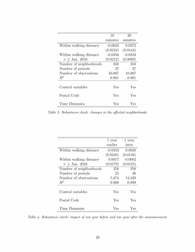
Table 3 presents the results of our baseline model of Table 2 in the case that we use two

different definitions of an affected area. The first new definition is based on a walking distance

18

of 10 minutes, while the second new definition looks at a walking distance of 20 minutes.

Note that this does not only affect the definition of the affected areas, but also the notion

of a comparison group. In general, the postal codes on which we base our identification,

i.e. those postal codes that have houses from both the affected and non-affected areas, are

at a longer distance from the building sites. This is reflected in the fact that the Within

walking distance dummy variable goes from insignificantly negative to significantly positive.

The impact of the building sites on the house price, i.e. the interacted dummy variable, is

less affected by the change in the definition. Still, we find the impact to be reducing with

distance. This is not surprising, since it can be argued that a 20-minute walking distance is

too far for the temporary building site to have a large impact.

6.2 Change in the timing of the impact on the building sites

Table 4 lists the results of our baseline model of Table 2 in the case that we forward or delay

the date of impact by one year. Naturally, the first exercise should not result in any impact

unless there is something wrong with the date that we have chosen or with the choice of

control and treatment group. The first column of Table 4 shows that there is indeed no

impact with a point estimator virtually equal to zero. It is also very unlikely that there is an

impact if we delay the date of the impact by one year. This implies that the dummy variable

Within walking distance is now a mixture of the period before January 2016 and the period

between January 2016 and January 2017. From our baseline results, we know that the first

period was slightly positive and since this period is the longest by far, it is not surprising

that the dummy variable is slightly positive as well. The impact variable of the temporary

building sites is still somewhat negative, but it is far from significant.

19

10 20minutes minutes

Within walking distance -0.0023 0.0373(0.0216) (0.0144)

Within walking distance -0.0356 -0.0234× ≥ Jan. 2016 (0.0212) (0.0089)

Number of neighborhoods 358 358Number of periods 37 37Number of observations 10,067 10,067R2 0.901 0.901

Control variables Yes Yes

Postal Code Yes Yes

Time Dummies Yes Yes

Table 3: Robustness check: changes in the affected neighborhoods.

1 year 1 yearearlier later

Within walking distance -0.0353 0.0028(0.0248) (0.0148)

Within walking distance 0.0017 -0.0082× ≥ Jan. 2016 (0.0179) (0.0125)



Postal Code Yes Yes


Table 4: Robustness check: impact of one year before and one year after the announcement.

20

6.3 Deletion of outliers

Table 5 shows the impact of our baseline results when we delete either 1 or 5 percent of the

lowest and highest prices in our sample. Even though we do not expect a huge amount of

measurement error in our analysis, it is still interesting to understand whether our results are

based on observations that are located at the edges of the support of the price distribution.

The point estimator in the case that we delete 1 percent of the highest and lowest prices is

somewhat lower than the point estimator reported in the first column of Table 2. However,

the difference is small and it does not really change our conclusions in a qualitative way.

That is, we still have a negative and significant impact of the temporary building sites.

This result changes whenever we delete the 5 percent highest and lowest prices in our data

set, respectively. The point estimator is reduced even further and becomes insignificant.

This result shows that our baseline results are somewhat affected by the choice of our data

set. Nevertheless, a deletion of 10 percent of the observations is quite drastic and it is not

surprising that the impact is not completely homogeneous with the price level.

6.4 Change in the control group

Our baseline model assumes that we can interpret the rest of Gothenburg, Partille and

Molndal as comparable to the affected areas in our analysis. This is an appropriate assump-

tion as long as the coefficients of the controls (including the time trend) do not differ to

any considerable extent between the affected and non-affected areas. However, especially

the (poorer) northern part of Gothenburg differs considerably from the temporary building

sites, which are located in prosperous areas in Gothenburg. Therefore, we use an alternative

estimation technique in this subsection, where we only include houses that are located no

further than a 60 minute walking distance from any of the temporary building sites. This

21

1 percent 5 percentdeleted deleted

Within walking distance -0.0373 -0.0006(0.0196) (0.0082)

Within walking distance -0.0288 -0.0196× ≥ Jan. 2016 (0.0139) (0.0176)



Postal Code Yes Yes


Table 5: Robustness check: changes in the affected neighborhoods.

excludes any of the poor neighborhoods in the northern part of Gothenburg, which can be

reached only by car or public transport (due to the river that divides the northern from the

southern part). The results of this exercise are listed in Table 6, where we have redone all

estimations of Table 2. Note that we lose around 60 percent of our observations by using this

approach. We find that the point estimator for our baseline model is negative and somewhat

smaller in absolute value than what was reported in Table 2. Although the difference is not

extreme, we also find that the coefficient is only significant in the case that we do not use

clustered standard errors. As discussed earlier, not correcting for clusters means that we

rule out strong heterogeneity in the impacts between the postal codes. Moreover, the results

for higher levels of aggregation are no longer significant even though we remind ourselves

that we have a strong preference for the low level of aggregation that we use in our baseline

analysis. Finally, the parallel trend assumption is not violated for this estimation strategy.

22

Baseline Baseline 4 digit 3 digit Parallel(5 digit (clustered postal postal trend

postal codes) stand. err.) codes codes


Within walking distance 0.0039× < Jan. 2016 (0.0162)

Within walking distance -0.0245 -0.0245 -0.0223 0.0090 -0.0229× ≥ Jan. 2016 (0.0135) (0.0181) (0.0171) (0.0193) (0.0153)

Number of neighborhoods 160 160 37 11 160Number of periods 37 37 37 37 37Number of observations 4,808 4,808 4,808 4,808 4,808R2 0.891 0.891 0.800 0.686 0.891

Control variables Yes Yes Yes Yes Yes

Postal Codes Yes Yes Yes Yes Yes


Table 6: Robustness check: restricted control group.

6.5 Extension of the time window

Up till now, we have only looked at the period one year after the announcement. Obviously,

this is the most important period for our analysis and it would be surprising if the (suspected)

impact of the announcement would have had a time lag that is longer than one year. Still, it

is interesting to investigate whether there was even an impact after a year. This is even more

important since it was announced in September 2017 that the temporary building sites of

Karralundsvallen and Lemmingsvallen were canceled due to the high costs of these building

sites. It implies that only the temporary building site of Askimsbadet was still planed after

September 2017. Moreover, the impact of this building site may be small due to the fact that

there are very few apartments within walking distance of this building site. Hence, even if

there is any impact, it is unlikely that we would pick it up in our baseline analysis. Therefore,

we look at two periods in Table 7: first the period from January 2016 to September 2017

23

and then the period from September 2017 to November 2017. The results from the same

specifications as Table 2 are reported in Table 7. The results for the period from January

2016 to September 2017 are surprisingly similar to the earlier reported results. However, the

impact after September 2017 is very small and far from significant.

6.6 Additional results for single-family houses

Our baseline results are only based on data from apartments which are relatively homoge-

neous. Nevertheless, it is interesting to investigate whether our results depend on this choice.

Therefore, Table 8 lists the results for single-family houses. We apply the same methods as

in the original Table 2, but we exclude floor and rent from the set of regressors. The results

are in line with our earlier results. The regression coefficient of the impact of the temporary

building sites is once more negative and even larger in absolute values than the results in

Table 2. Apart from our baseline regression, the results are also significant at the 10 percent

level. Based on these results, it is not possible to say that this contradicts our earlier results,

even though the standard errors are somewhat too large to say that these results underline

the earlier results.

In contrast to apartments, transactions of single-family houses are registered in Sweden

and hence, it is interesting to investigate the impact of measurement error in the Booli

dataset. That is, we can investigate the fact that some houses may not have been sold even

after a final bid or they might have been sold, but at a substantially lower price. For this

purpose, we merge our dataset with the records from the Swedish register. Unfortunately, we

do not have a common registration number, nor do we have the exact address of the houses.

Therefore, we decided to merge on basis of the GPS codes. We use the first six digits for this

purpose. Based on this, we were not able to match 698 observations. This can be due to a

24





Within walking distance -0.0242 -0.0242 -0.0218 0.0017 -0.0195× ≥ Jan. 2016-Sept. 2017 (0.0120) (0.0148 ) (0.0143) (0.0155) (0.0148)

Within distance -0.0091 -0.0091 0.0116 0.0047 -0.0039× ≥ Sept. 2017 (0.0243) (0.0181 ) (0.0266) (0.0361) (0.0260)





Table 7: Robustness check: longer time period.

25



Within walking distance -0.0061 -0.0061 -0.0011 0.1715 -0.0185(0.0342) (0.0412) (0.0275) (0.0289) (0.0185)


Within walking distance -0.0735 -0.0735 -0.0816 -0.1034 -0.0660× ≥ Jan. 2016-Jan. 2017 (0.0470) (0.0201) (0.0488 ) (0.0522) (0.0532)





Table 8: Robustness check: single-family houses after deletion of houses that were not merged withdata from the register.

gap in the GPS coding, but it is also possible that some houses were not sold or were sold,

but the change of ownership was after the period for which we have data (January 2017).9 In

addition, we also delete observations with a change in ownership before the transaction date

on Booli. Such a transaction typically indicates that there were multiple transactions and

the reported transaction on Booli was simply after the previous change of ownership. We

also delete observations with a change in ownership one year or more after the transaction

date from Booli or when the price on Booli does not match the price that was reported

by the register. All these filters resulted in a deletion of 380 observations. The results of

this exercise are reported in Table 9. We find that the results for the baseline analysis are

not changed to any large extent, while the change in the other columns is somewhat larger.

However, the large standard errors frustrate any definite conclusion here, most likely due to

9In fact, we had to do a recoding since the GPS coding of the register uses a coding system calledSWEREF99 which was not used by the Booli website.

26

the low number of observations.

7 Discussion

The previous sections have shown evidence for a reduction in the apartment prices as a result

of the announcement of the temporary building sites in the affected areas. In this section, we

investigate some potential explanations for the drop in the apartment prices. Our preferred

interpretation of the results is that supply effects did not play a large role since the houses

that were planned to be built are unlikely to compete with the apartments that were for sale

after the announcement of the temporary building sides. That is, prospective buyers of the

apartments cannot buy a house in the temporary building sites, while it is unlikely to be the

case that the municipality would have bought these (in general quite expensive) apartments

for the housing of refugees in the case that the temporary building sites would not have been

announced. This implies that the houses to be build on the temporary building sites are part

of another market than the apartments that we investigate. Hence, if anything, it would

reduce the prospective supply of apartments in these areas by reducing the opportunities

for developers to buy the land in the future. However, that would have resulted in a price

increase rather than a decrease. Therefore, it is more likely that demand effects have played

a role. That is, the announcement of the temporary building sites lowered demand for the

areas that were close to these sites since prospective buyers were averse to living close to

the temporary building sites. Still, it is possible that the extent of the preference to live

close to these sites depends on the attributes of the current and prospective residents as

well as the characteristics of the neighborhood. In order to investigate this, we look at

the impact of the number of existing immigrants, the education and the income level of

the neighborhoods involved. For this purpose, we matched our dataset with data from the

27





Within walking distance -0.0596 -0.0596 -0.0297 -0.0306 -0.0428× ≥ Jan. 2016-Jan. 2017 (0.0800) (0.0802) (0.0648) (0.0488 ) (0.0835)





Table 9: Robustness check: single-family houses.

database of the municipality of Gothenburg and use the definition of primary neighborhoods

(primaromraden) which divides Gothenburg into 94 different neighborhoods. All our data

is for the year 2016.

In order to investigate the impact of immigrants, we calculate the percentage of individu-

als in between 19 and 65 years of age who are born outside of Sweden and divide this by the

total number of individuals within this age category who live in the neighborhood. Then,

we use two different indicators for immigrant neighborhoods, those with more than 10 and

those with more than 25 percent immigrants. In general, the impact of immigrants is not

that clear a priori. Since the number of houses that is to be built in any of the temporary

building sites is not that high in comparison to the present housing stock, it is not to be

expected that the relative number of immigrants is changing a lot due to the building of

these housing sites. Hence, it is possible that areas that do not have a lot of immigrants

28

are not affected by a large extent since the immigrants are still going to be in far minority.

Economic theory states that the likelihood of integration of small groups is very high (Ad-

vani and Reich, 2015). On the other hand, going from a percentage of immigrants that is far

below 10 percent (as is the case in many areas around Askimsbadet), to a percentage that is

somewhat higher can at least psychologically be seen as a large difference, while going from

a percentage well above 25 percent to a little bit higher can be interpreted as not a large

difference at all.

Table 10 lists the results of our exercise. The first column reports the results of a re-

gression with the 10 percent immigrants dummy variable as an additional variable. This

column is introduced to compare it with our baseline results. Our results are not affected

by any extend and we find a negative impact of the dummy variable of having more than

10 percent immigrants on the apartment price. Note that the sign and size of this dummy

variable cannot be interpreted as causal as many unobserved neighborhood characteristics

may be correlated with the number of immigrants residing in a particular neighborhood. The

second column lists the main effects and shows that as soon as the percentage of immigrants

is larger than 10 percent, then the impact is much smaller and only significantly different

from zero for a significance level of 10 percent.10 This suggests that our results are mainly

driven by Swedish native buyers who prefer to be living in areas with a population that

is almost entirely from a Swedish background. Prospective buyers who buy houses closer

to immigrant dense neighborhoods seem not highly affected by the announcement of the

temporary building sides. The third column presents results of a similar regression but here

we also investigate the impact of neighborhoods with at least 25 percent of immigrants. We

find here an even larger positive impact for the severely mixed neighborhoods even though

the results are not statistically significant.

10The t-value (not reported here) equals 1.64.

29

Baseline Immigration Immigration rate+ immigration rate > 10% ≥ 10 % and

rate ≥ 25 %

Within walking distance -0.0003 0.0709 0.0923(0.0190) (0.0550) (0.0558)

Within walking distance -0.0747 -0.0973× Immigration rate ≥ 10% (0.0536) (0.0547)

Within walking distance -0.0150× Immigration rate ≥ 25% (0.0384)

Within walking distance -0.0317 -0.0444 -0.0449× ≥ Jan. 2016-Jan. 2017 (0.0136) (0.0244) (0.0249)

Within walking distance 0.0178 0.0143× ≥ Jan. 2016-Jan. 2017 (0.0289) (0.0297)× Immigration rate ≥ 10%

Within walking distance 0.0514× ≥ Jan. 2016-Jan. 2017 (0.0493)× Immigration rate ≥ 25%

Immigration rate ≥ 10% -0.0404 0.0165 0.0394(0.0216) (0.0459) (0.0478)

Immigration rate ≥ 25% -0.0276(0.0081)

Number of neighborhoods 220 220 220Number of periods 37 37 37Number of observations 10,067 10,067 10,067R2 0.901 0.901 0.901

Control variables Yes Yes Yes

Postal Code Yes Yes Yes

Time Dummies Yes Yes Yes

Table 10: Discussion: including the migration rate in the analysis.

30

Our second exercise is to investigate the impact of education on the price impact of

the temporary building sites. We look at education levels within the neighborhood for the

population in between 25 and 65 years of age.11 From the ethnic and migration literature,

it is known that higher levels of education typically reduce negative prejudice with respect

to foreigners and hence we expect education to reduce the impact of the temporary building

sites (see for example Hjerm, 2001). Also, it is suggested in the popular literature in Sweden

that especially the lower educated are more likely to vote in favor of the anti-immigration

party.12 Here we use a dummy variable in the case that the neighborhood is ranked below the

median of neighborhoods in terms of education level. The results of this exercise are listed

in Table 11. The first column is again the baseline regression but now with the education

dummy included. Low education levels in a neighborhood have a large negative impact on the

apartment prices but again this can be interpreted as an effect of unobserved neighborhood

characteristics rather than the presence of high educated individuals themselves. In the

second column, we find, somewhat surprisingly, that a low level of education decreases the

impact of the temporary building sites but the results are not significant. It is important

to notice that this may be due to the fact that education is correlated with migration rates

in the sense that low migration areas are typically areas with on average high education

levels. Therefore, we include our immigration dummy together with the education levels

in the third column of Table 11. Again, it is difficult to draw strong conclusions from this

column, but we find that it is definitely not the case that low levels of education correlate

with bigger impacts of the temporary building sites.

As a final exercise, we look at the impact of income on the price effect of temporary

building sites by including a dummy that equals one in the case that the median income

11Education levels are calculated in years of education, based on the highest grade obtained.12See Aftonbladet, May, 26th, 2014.

31

Baseline Education Immigration rate+ education level + education

level level

Within walking distance 0.0039 0.0011 0.0152(0.0191) (0.0200) (0.0549)

Within walking distance -0.0062 0.0164× Education below median (0.0253) (0.0304)



Within walking distance 0.0208 0.0115× ≥ Jan. 2016-Jan. 2017 (0.0274) (0.0376)× Education below median


Education level below median -0.0412 -0.0416 -0.0419(0.0080) (0.0086) (0.0086)






Table 11: Discussion: including the neighborhood education level in the analysis.

32

is ranked among the 50 percent lowest medians over all neighborhoods. The results of

this exercise are listed in Table 12. Again, the first column is for comparison where we

include the dummy variable in the baseline analysis. The results are not affected to any

large extent and the income dummy variable has an unsurprisingly negative impact on the

price of the house. The second column extents our baseline by investigating the impact of

the announcement in terms of the house price for different income levels. Even though the

overall impact is negative and significant, the impact is insignificant and positive for low

income neighborhoods. This is identical to the statement that our results are driven by

above median income neighborhoods. Column 3 of Table 12 also includes education level

and immigration rate into the analysis. We find these neighborhood characteristics to be of

minor importance than income. Hence, our interpretation of the results is that not having

to live close to refugees can be seen as a luxury good in a hedonic framework of housing

characteristics. That is, for lower incomes, there are likely to be other characteristics that

drive the value of the apartment, but as soon as individuals obtain a certain level of income,

then having the opportunity not to live close to refugees becomes more important. We

cannot speculate whether this is caused by high-income house buyers to be unwilling to buy

houses close to immigrants or that they are only reluctant to buy a house close to refugees.

We can equally not speculate whether these results are driven by a taste to live distant

from refugees (or immigrants in general) or whether it is just a concern of the high-income

buyers that their prospective investment might lose value. Again, we find education not to

play any role: if anything, individuals in high-educated neighborhoods have the tendency

to care even more about the negative impact of a potential high concentration of refugees

on the neighborhood’s apartment prices. Note that this is not necessarily in contrast with

the earlier mentioned observation that the lowly educated are more likely to vote for anti-

33

migration parties. The highly educated have typically a high level of income and they can

overcome the effects of high migration rates simply by living in areas with low concentrations

of migrants. Hence, for these highly educated having high migration rates is not really an

issue when it comes to their voting behavior. On the contrary, such behavior is impossible

for the lowly educated. Also, the number of immigrants does not seem to play a role, but we

should notice that high-income neighborhoods do not have a lot of immigrants in the first

place.

8 Conclusions

This paper investigated whether property prices nearby temporary housing sites were affected

after the announcement of the sites by using an empirical model with both postal code and

time effects. We define the affected neighborhoods based on walking distance. The results

suggest that the market for apartments has experienced a negative effect, although some of

the robustness checks were insignificant.

Our results are especially interesting since the temporary building sites were not built

during our observation window and, as it turned out, the majority of the building sites (2 out

of 3) are not going to be built either. This implies that potential house buyers are forward

looking and that only an announcement of a building site can even result in substantial price

losses of the houses around that building site. Thus, this implies that governments should

be careful with their announcements.

34

Baseline Income Income ++ income level education level

level + immigration rate

Within walking distance 0.0043 0.0006 0.0176(0.0191) (0.0211) (0.0554)

Within walking distance 0.0286 -0.0238× Income below median (0.0328) (0.0335)

Within walking distance 0.0131× Education below median (0.0306)



Within walking distance 0.1508 0.1475× ≥ Jan. 2016-Jan. 2017 (0.0824) (0.0827)× Income below median

Within walking distance 0.0061× ≥ Jan. 2016-Jan. 2017 (0.0377)× Education below median


Below median income -0.0279 -0.0280 -0.0111(0.0108) (0.0108) (0.0101)

Education level below median -0.0378(0.0090)






Table 12: Discussion: including the neighborhood income level in the analysis.

35

References

Abadie, A. S. Athey, G. Imbens and J. Wooldridge (2017), “When should you adjust

standard errors for clustering?”, working paper, Massachusetts Institute of Technology,

Cambridge (MA)

Advani, A. and B. Reich (2015), “Melting pot or salad bowl: the formation of heteroge-

neous communities”, working paper, University College London.

Bejenariu, S., and Mitrut, A. (2013), “Austerity measures and infant health. Lessons

from an unexpected wage cut policy”, working paper, University of Gothenburg.

Gautier, P. A., A. Siegmann, A., and A.P. Van Vuuren (2009), “Terrorism and

attitudes towards minorities: The effect of the Theo van Gogh murder on house prices

in Amsterdam”, Journal of Urban Economics, 65, 113-26.

Goteborg Stad (2016), “Temporra bostader”, report, Gothenburg.

Hjalmarsson, E. and R.. Hjalmarsson (2009), “Efficiency in housing markets: which

home buyers know how to discount?”, Journal of Banking and Finance, 33, 2150-63.

Hjerm, M. (2010), “Education, xenophobia and nationalism: A comparative analysis”,

Journal of Ethnic and Migration Studies, 27, 37–60.

Lastrapes, W.D and T. Lebesmuehlbacher (2016), “The European refugee crisis

and house prices: evidence from the United Kingdom ”, working paper, University of

Georgia, Athens (GA).

Saiz, A. (2007). “Immigration and housing rents in American cities ”. Journal of Urban

Economics, 61, 345–71.

36

Saiz, A., and Wachter, S. (2011). “Immigration and the neighborhood”, American

Economic Journal: Economic Policy, 3, 16988.

Sa, F. (2015), “Immigration and house prices in the UK ”, Economic Journal, 125, 1393-

1424 .

Appendix

Table 13: Variable definition and sources

Variable Description Source

Price The price at which the property was sold, in thousand SEK. Booli.se, Lantmateriet

Square meter price Price/Living area Booli.se, Lantmateriet

DistanceDistance to closest refugee site expressed in kilometers, calculated using

Booli.se, Lantmaterietcoordinates in the WGS 84 and SWEREF 99 standard

WithinBinary variable, 1 if property located within a threshold cut-off distance - Booli.se, Goteborg.se,

(0.5, 1 or 1,5 kilometer) of a refugee site, 0 otherwise Lantmateriet

PostDummy variable indicating 1 if the month of sale was after the announcement Booli.se, Goteborg.se

of placement of refugee sites, 0 otherwise. Lantmateriet

Living area Surface of property measured in square meters. Booli.se, Lantmateriet

Construction year Year construction of the property was finished. Booli.se, Lantmateriet

Floor Floor on which the apartment is located in the building. Booli.se

Rent Monthly rent paid to the building association. Booli.se

Yearly rent/m2 (Rent ∗ 12)/Living area. Booli.se

Rooms Number of rooms in the apartment excluding kitchen and bathroom(s). Booli.se

m2/rooms Living area/Rooms. Booli.se

Additional areaArea connected to the house but not defined as Living area,

Lantmateriete.g. Basement and garage

House type Category of housetype where villa=1, chain house=2 and town house=3. Lantmateriet

Lot size Size of lot on which the single-family house is situated in square meters. Lantmateriet

Value pointsA measure of points for the standard of the single-family house,

Lantmaterietbased on the buildings material and equipment.

Waterfront house Dummy variable, 1 if house is situated within 150 meters to the shoreline, 0 otherwise Lantmateriet

Postal codePostal code. Specified as a 5-digit postal code

Booli.se, Lantmaterietor as 4- or 3-digit code, using the first 3 or 4 digits of the postal code.

Time On a monthly basis. Ranges from January 2014 to February 2017. Booli.se, Lantmateriet

37

Figure 3: Location of sites - East

Figure 4: Location of sites - West

38

Documents

DISUSSIN PAP SIS - ftp.iza.orgftp.iza.org/dp11726.pdf · method as Saiz and Wachter (2011) using the UK labor force survey. She concludes that a 1 She concludes that a 1 percent increase