Diversi cation Reconsidered: Minimum Tail Dependency · Diversi cation Reconsidered: Minimum Tail Dependency ... 6th R/Rmetrics Meielisalp Workshop ... Utilization in Optimization

Diversification Reconsidered:Minimum Tail Dependency

Bernhard [email protected]

Invesco Asset Management Deutschland GmbH, Frankfurt am Main

6th R/Rmetrics Meielisalp WorkshopJune 24 –28, 2012

Meielisalp, Lake Thune Switzerland

Pfaff (Invesco) Diversification R/Rmetrics 1 / 24

Contents

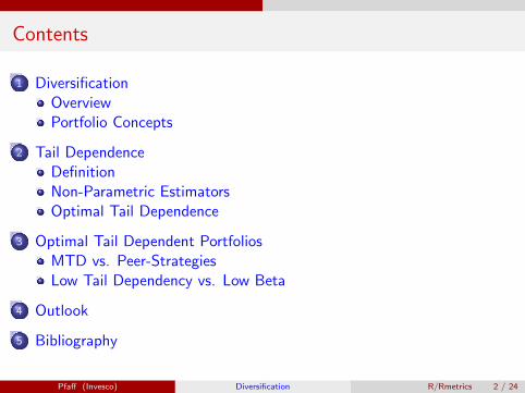
1 DiversificationOverviewPortfolio Concepts

2 Tail DependenceDefinitionNon-Parametric EstimatorsOptimal Tail Dependence

3 Optimal Tail Dependent PortfoliosMTD vs. Peer-StrategiesLow Tail Dependency vs. Low Beta

4 Outlook

5 Bibliography


Diversification Overview

DiversificationOverview

60th anniversary of MPT (see Markowitz, 1952)

Reducing risk by investing in a variety of assets

At least two scopes of the word ‘diversification’

Divers with respect to what?How to measure diversification?


Diversification Portfolio Concepts

DiversificationPortfolio Concepts: The Peers

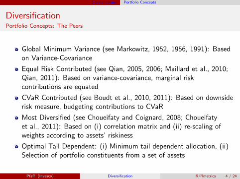
Global Minimum Variance (see Markowitz, 1952, 1956, 1991): Basedon Variance-Covariance

Equal Risk Contributed (see Qian, 2005, 2006; Maillard et al., 2010;Qian, 2011): Based on variance-covariance, marginal riskcontributions are equated

CVaR Contributed (see Boudt et al., 2010, 2011): Based on downsiderisk measure, budgeting contributions to CVaR

Most Diversified (see Choueifaty and Coignard, 2008; Choueifatyet al., 2011): Based on (i) correlation matrix and (ii) re-scaling ofweights according to assets’ riskiness

Optimal Tail Dependent: (i) Minimum tail dependent allocation, (ii)Selection of portfolio constituents from a set of assets


Tail Dependence Definition

Tail DependenceDefinition (i)

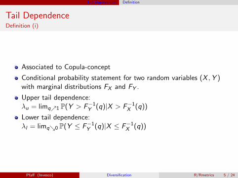
Associated to Copula-concept

Conditional probability statement for two random variables (X ,Y )with marginal distributions FX and FY .

Upper tail dependence:λu = limq↗1 P(Y > F−1

Y (q)|X > F−1X (q))

Lower tail dependence:λl = limq↘0 P(Y ≤ F−1

Y (q)|X ≤ F−1X (q))


Tail Dependence Definition

Tail DependenceDefinition (ii)

Expressed in Copula-terms:

Upper tail dependence:λu = 2 + limq↘0

C(1−q,1−q)−1q

Lower tail dependence:λl = limq↘0

C(q,q)q

Student’s t Copula:λu = λl = 2tν+1(−

√ν + 1

√(1− ρ)/(1 + ρ))

Archimedean Copulae:

Gumbel Copula: λu = 2− 21/θ

Clayton Copula: λl = 2−1/δ


Tail Dependence Non-Parametric Estimators

Tail DependenceNon-Parametric Estimators (i)

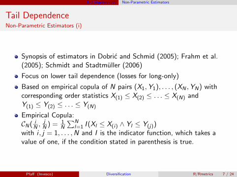
Synopsis of estimators in Dobric and Schmid (2005); Frahm et al.(2005); Schmidt and Stadtmuller (2006)

Focus on lower tail dependence (losses for long-only)

Based on empirical copula of N pairs (X1,Y1), . . . , (XN ,YN) withcorresponding order statistics X(1) ≤ X(2) ≤ . . . ≤ X(N) andY(1) ≤ Y(2) ≤ . . . ≤ Y(N)

Empirical Copula:CN( i

N ,jN ) = 1

N

∑Nl=1 I (Xl ≤ X(i) ∧ Yl ≤ Y(j))

with i , j = 1, . . . ,N and I is the indicator function, which takes avalue of one, if the condition stated in parenthesis is true.


Tail Dependence Non-Parametric Estimators

Tail DependenceNon-Parametric Estimators (ii)

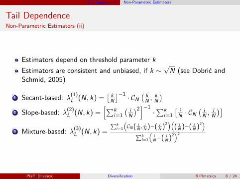
Estimators depend on threshold parameter k

Estimators are consistent and unbiased, if k ∼√N (see Dobric and

Schmid, 2005)

1 Secant-based: λ(1)L (N, k) =

[kN

]−1 · CN

(kN ,

kN

)2 Slope-based: λ

(2)L (N, k) =

[∑ki=1

(iN

)2]−1·∑k

i=1

[iN · CN

(iN ,

iN

)]3 Mixture-based: λ

(3)L (N, k) =

∑ki=1

(CN( i

N, i

N )−( iN )

2)(

( iN )−( i

N )2)

∑ki=1

(iN−( i

N )2)2


Tail Dependence Optimal Tail Dependence

Tail DependenceUtilization in Optimization

Minimum Tail Dependent Portfolio

Approach similar to MDPFirst step: Derive optimal solution if TDC-matrix is used withmain-diagonal elements are set to one.Second step: Re-scale optimal weight vectors by assets volatility(riskiness).Implemented in package FRAPO (see Pfaff, 2012)

Asset Selection

Benchmark-relative OptimisationsChoose constitutents which are least lower tail dependent to thebenchmark (index).No implication with respect to the upper tail dependencies, in contrastto low β strategies that are in general based on a symmetricco-dispersion measure.


Optimal Tail Dependent Portfolios MTD vs. Peer-Strategies

MTD vs. Peer-StrategiesOverview

Swiss Performance Sector Indexes

Static long-only optimisation according to

GMVMDPERCMTD

Analysis of allocations, risk- & marginal risk contributions, and keymeasures



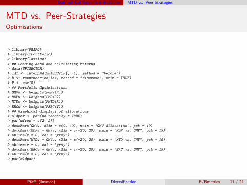
MTD vs. Peer-StrategiesOptimisations

> library(FRAPO)

> library(fPortfolio)

> library(lattice)

> ## Loading data and calculating returns

> data(SPISECTOR)

> Idx <- interpNA(SPISECTOR[, -1], method = "before")

> R <- returnseries(Idx, method = "discrete", trim = TRUE)

> V <- cov(R)

> ## Portfolio Optimisations

> GMVw <- Weights(PGMV(R))

> MDPw <- Weights(PMD(R))

> MTDw <- Weights(PMTD(R))

> ERCw <- Weights(PERC(V))

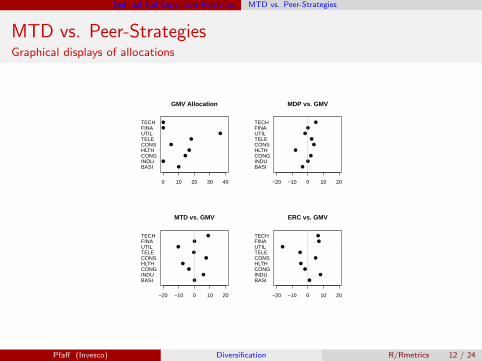
> ## Graphical displays of allocations

> oldpar <- par(no.readonly = TRUE)

> par(mfrow = c(2, 2))

> dotchart(GMVw, xlim = c(0, 40), main = "GMV Allocation", pch = 19)

> dotchart(MDPw - GMVw, xlim = c(-20, 20), main = "MDP vs. GMV", pch = 19)

> abline(v = 0, col = "gray")

> dotchart(MTDw - GMVw, xlim = c(-20, 20), main = "MTD vs. GMV", pch = 19)


> dotchart(ERCw - GMVw, xlim = c(-20, 20), main = "ERC vs. GMV", pch = 19)


> par(oldpar)



MTD vs. Peer-StrategiesGraphical displays of allocations

BASIINDUCONGHLTHCONSTELEUTILFINATECH

●

●

●

●

●

●

●

●

●

0 10 20 30 40

GMV Allocation


●

●

●

●

●

●

●

●

●

−20 −10 0 10 20

MDP vs. GMV


●

●

●

●

●

●

●

●

●

−20 −10 0 10 20

MTD vs. GMV


●

●

●

●

●

●

●

●

●

−20 −10 0 10 20

ERC vs. GMV



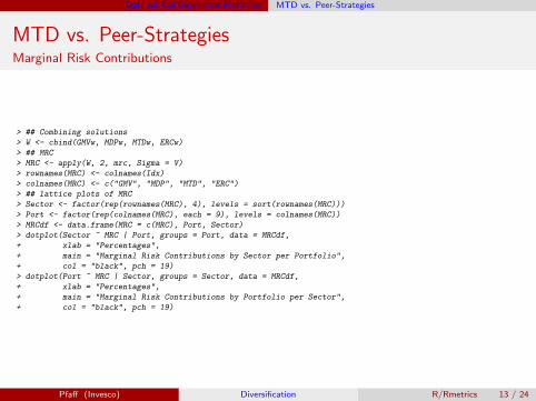
MTD vs. Peer-StrategiesMarginal Risk Contributions

> ## Combining solutions

> W <- cbind(GMVw, MDPw, MTDw, ERCw)

> ## MRC

> MRC <- apply(W, 2, mrc, Sigma = V)

> rownames(MRC) <- colnames(Idx)

> colnames(MRC) <- c("GMV", "MDP", "MTD", "ERC")

> ## lattice plots of MRC

> Sector <- factor(rep(rownames(MRC), 4), levels = sort(rownames(MRC)))

> Port <- factor(rep(colnames(MRC), each = 9), levels = colnames(MRC))

> MRCdf <- data.frame(MRC = c(MRC), Port, Sector)

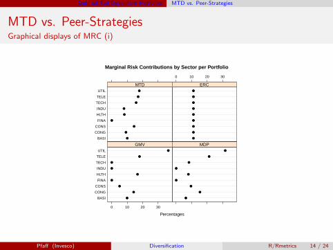
> dotplot(Sector ~ MRC | Port, groups = Port, data = MRCdf,

+ xlab = "Percentages",

+ main = "Marginal Risk Contributions by Sector per Portfolio",

+ col = "black", pch = 19)

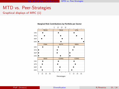
> dotplot(Port ~ MRC | Sector, groups = Sector, data = MRCdf,

+ xlab = "Percentages",

+ main = "Marginal Risk Contributions by Portfolio per Sector",

+ col = "black", pch = 19)



MTD vs. Peer-StrategiesGraphical displays of MRC (i)

Marginal Risk Contributions by Sector per Portfolio

Percentages

BASI

CONG

CONS

FINA

HLTH

INDU

TECH

TELE

UTIL

0 10 20 30

●

●

●

●

●

●

●

●

●

GMV

●

●

●

●

●

●

●

●

●

MDP

BASI

CONG

CONS

FINA

HLTH

INDU

TECH

TELE

UTIL

●

●

●

●

●

●

●

●

●

MTD

0 10 20 30

●

●

●

●

●

●

●

●

●

ERC



MTD vs. Peer-StrategiesGraphical displays of MRC (ii)

Marginal Risk Contributions by Portfolio per Sector

Percentages

GMV

MDP

MTD

ERC

0 10 20 30

●

●

●

●

BASI

●

●

●

●

CONG

0 10 20 30

●

●

●

●

CONS

GMV

MDP

MTD

ERC

●

●

●

●

FINA

●

●

●

●

HLTH

●

●

●

●

INDU

GMV

MDP

MTD

ERC

●

●

●

●

TECH

0 10 20 30

●

●

●

●

TELE

●

●

●

●

UTIL



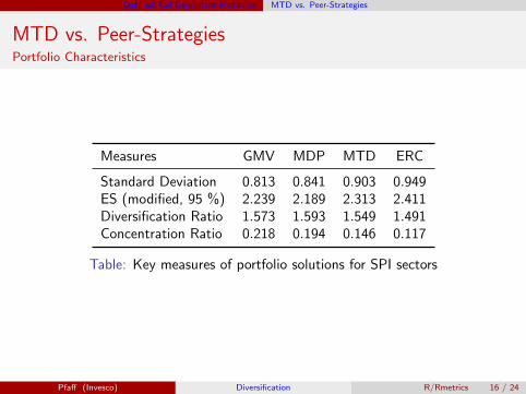
MTD vs. Peer-StrategiesPortfolio Characteristics

Measures GMV MDP MTD ERC

Standard Deviation 0.813 0.841 0.903 0.949ES (modified, 95 %) 2.239 2.189 2.313 2.411Diversification Ratio 1.573 1.593 1.549 1.491Concentration Ratio 0.218 0.194 0.146 0.117

Table: Key measures of portfolio solutions for SPI sectors


Optimal Tail Dependent Portfolios Low Tail Dependency vs. Low Beta

Low Tail Dependency vs. Low BetaOverview

Benchmark relative optimisation: S&P 500

Weekly data: 291 observations of the index and 457 constituents.The sample starts in March 1991 and ends in September 1997.Source: INDTRACK6 (OR-Library)

Long-only portfolio, in-sample period 260 observations

Similar analysis in Malevergne and Sornette (2008)



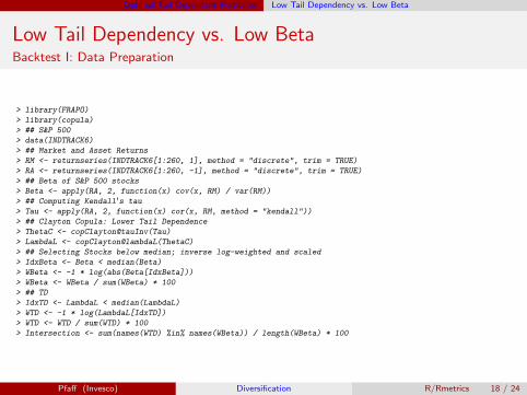
Low Tail Dependency vs. Low BetaBacktest I: Data Preparation

> library(FRAPO)

> library(copula)

> ## S&P 500

> data(INDTRACK6)

> ## Market and Asset Returns

> RM <- returnseries(INDTRACK6[1:260, 1], method = "discrete", trim = TRUE)

> RA <- returnseries(INDTRACK6[1:260, -1], method = "discrete", trim = TRUE)

> ## Beta of S&P 500 stocks

> Beta <- apply(RA, 2, function(x) cov(x, RM) / var(RM))

> ## Computing Kendall's tau

> Tau <- apply(RA, 2, function(x) cor(x, RM, method = "kendall"))

> ## Clayton Copula: Lower Tail Dependence

> ThetaC <- copClayton@tauInv(Tau)

> LambdaL <- copClayton@lambdaL(ThetaC)

> ## Selecting Stocks below median; inverse log-weighted and scaled

> IdxBeta <- Beta < median(Beta)

> WBeta <- -1 * log(abs(Beta[IdxBeta]))

> WBeta <- WBeta / sum(WBeta) * 100

> ## TD

> IdxTD <- LambdaL < median(LambdaL)

> WTD <- -1 * log(LambdaL[IdxTD])

> WTD <- WTD / sum(WTD) * 100

> Intersection <- sum(names(WTD) %in% names(WBeta)) / length(WBeta) * 100



Low Tail Dependency vs. Low BetaBacktest II: Out-of-sample

> ## Out-of-Sample Performance

> RMo <- returnseries(INDTRACK6[260:290, 1], method = "discrete",

+ percentage = FALSE) + 1

> RAo <- returnseries(INDTRACK6[260:290, -1], method = "discrete",

+ percentage = FALSE) + 1

> ## Benchmark

> RMo[1] <- 100

> RMEquity <- cumprod(RMo)

> ## Low Beta

> LBEquity <- RAo[, IdxBeta]

> LBEquity[1, ] <- WBeta

> LBEquity <- rowSums(apply(LBEquity, 2, cumprod))

> ## TD

> TDEquity <- RAo[, IdxTD]

> TDEquity[1, ] <- WTD

> TDEquity <- rowSums(apply(TDEquity, 2, cumprod))



Low Tail Dependency vs. Low BetaBacktest III: Progression of Portfolio Equity

> ## Collecting results

> y <- cbind(RMEquity, LBEquity, TDEquity)

> ## Time series plots of equity curves

> plot(RMEquity, type = "l", ylim = range(y), ylab = "Equity Index",

+ xlab = "Out-of-Sample Periods")

> lines(LBEquity, col = "green")

> lines(TDEquity, col = "blue")

> legend("topleft", legend = c("S&P 500", "Low Beta", "Lower Tail Dep."),

+ col = c("black", "green ", "blue"))

> ## Bar plot of out-performance

> RelOut <- rbind((LBEquity / RMEquity - 1) * 100,

+ (TDEquity / RMEquity - 1) * 100)

> RelOut <- RelOut[, -1]

> barplot(RelOut, beside = TRUE, ylim = c(-5, 17), names.arg = 1:ncol(RelOut),

+ legend.text = c("Low Beta", "Lower Tail Dep."),

+ args.legend = list(x = "topleft"))

> abline(h = 0)

> box()



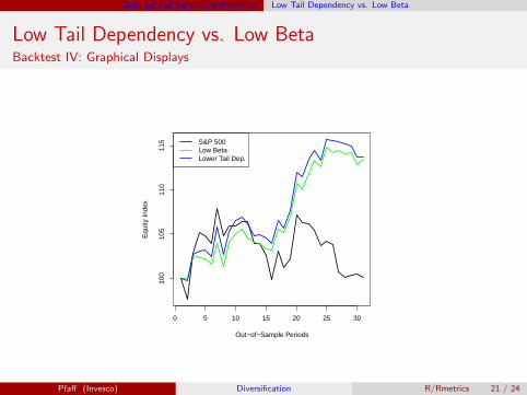
Low Tail Dependency vs. Low BetaBacktest IV: Graphical Displays

0 5 10 15 20 25 30

100

105

110

115

Out−of−Sample Periods

Equ

ity In

dex

S&P 500Low BetaLower Tail Dep.



Low Tail Dependency vs. Low BetaBacktest IV: Graphical Displays

1 3 5 7 9 11 14 17 20 23 26 29

Low BetaLower Tail Dep.

−5

05

1015


Outlook

OutlookExtension and Modifications

Use lower-partial moments for re-scaling of weights

Use upper- /lower TD ratio for optimization

Adapt approach to long-/short strategies


Bibliography

Bibliography I

Boudt, K., P. Carl, and B. Peterson (2010, April). Portfolio optimization with cvar budgets. Presentation at r/financeconference, Katholieke Universteit Leuven and Lessius, Chicago, IL.

Boudt, K., P. Carl, and B. Peterson (2011, September). Asset allocation with conditional value-at-risk budgets. Technicalreport, http://ssrn.com/abstract=1885293.

Choueifaty, Y. and Y. Coignard (2008). Toward maximum diversification. Journal of Portfolio Management 34(4), 40–51.

Choueifaty, Y., T. Froidure, and J. Reynier (2011). Properties of the most diversified portfolio. Working paper, TOBAM.

Dobric, J. and F. Schmid (2005). Nonparametric estimation of the lower tail dependence λl in bivariate copulas. Journal ofApplied Statistics 32(4), 387–407.

Frahm, G., M. Junker, and R. Schmidt (2005). Estimating the tail dependence coefficient: Properties and pitfalls. Insurance:Mathematics and Economics 37(1), 80–100.

Maillard, S., T. Roncalli, and J. Teiletche (2010). The properties of equally weighted risk contribution portfolios. The Journal ofPortfolio Management 36(4), 60–70.

Malevergne, Y. and D. Sornette (2008). Extreme Financial Risks – From Dependence to Risk Management. Berlin, Heidelberg:Springer-Verlag.

Markowitz, H. (1952, March). Portfolio selection. The Journal of Finance 7(1), 77–91.

Markowitz, H. (1956). The optimization of a quadratic function subject to linear constraints. Naval Research LogisticsQuarterly 3(1–2), 111–133.

Markowitz, H. (1991). Portfolio Selection: Efficient Diversification of Investments (2nd ed.). Cambridge, MA: Basil Blackwell.

Pfaff, B. (2012). Financial Risk Modelling and Portfolio Optimisation with R. London: Jon Wiley & Sons, Ltd. (forthcoming).

Qian, E. (2005). Risk parity portfolios: Efficient portfolios through true diversification. White paper, PanAgora, Bostan, MA.

Qian, E. (2006). On the financial interpretation of risk contribution: Risk budgets do add up. Journal of InvestmentManagement 4(4), 1–11.

Qian, E. (2011, Spring). Risk parity and diversification. The Journal of Investing 20(1), 119–127.

Schmidt, R. and U. Stadtmuller (2006). Nonparametric estimation of tail dependence. The Scandinavian Journal ofStatistics 33, 307–335.


Documents

Diversi cation Reconsidered: Minimum Tail Dependency · Diversi cation Reconsidered: Minimum Tail Dependency ... 6th R/Rmetrics Meielisalp Workshop ... Utilization in Optimization