Division rings and theory of equationsby Vivek Mukundan

Vivekananda College, ChennaiGuide : Professor B.Sury

This was the second part of a report on the project done under the JNCASRSummer Fellowship in May-June 2006 in I.S.I.Bangalore

In the first report, I had described the structure theory of semisimple ringsand modules and its applications to matrix groups. As mentioned there, thestructure theory isolates the division rings as basic objects of study fromwhich semisimple rings are built. Here, I start by studying some aspectsof division algebras. After discussing a number of interesting characteriza-tions of commutativity due to Herstein, Jacobson and to Wedderburn etc.,the Cartan-Brauer-Hua theorem and the fundamental Skolem-Noether the-orem are proved. Following this, the theory of equations over division ringsis studied. Results due to Gordon, Motzkin, Bray, Whaples and Niven aredemonstrated. Finally, Vandermonde matrices over division rings are dis-cussed culminating in a beautiful result of Lam on their invertibility whoseproof uses the ideas above.

1

§ Division rings and commutativity theorems

Recall that a division ring D is a (not necessarily commutative) ring withunity in which the set D∗ of non-zero elements is a group under the mul-tiplication of D. Of course, all fields are division rings. The most familiarexample of a division ring which is not a field is that of Hamilton’s realquaternions

H = a0 + a1i + a2j + a3k : ai ∈ R.Note in this example, H contains R as constant quaternions a0. Thus, Hcontains the field R as a subring which is contained in its center; this isreferred to as an R-algebra. In general, if D is a division ring, its center is afield k, and D is a simple (as a ring) k-algebra. One calls D central simpleover a field K if its center is K. In this section, we start by studying variousproperties of division rings which force commutativity. Following that, wediscuss the famous result of Frobenius which classifies all the possible divisionrings with center R. Then, we also prove the important Skolem-Noethertheorem.

Examples :

(i) General quaternion algebra.If a, b ∈ Q∗, the generalized quaternion algebra D(a, b) is defined as follows.Consider formal symbols i, j, k with i2 = a, j2 = b, ij = k = −ji. One canconsider the Q-algebra generated by i, j; that is,

D(a, b) = a0 + aii + a2j + a3k.The multiplication is dictated by the multiplication of the symbols i, j above.Note in particular that k2 = −ab. Then D(a, b) is a division algebra if, andonly if, the equation ax2 + by2 = 1 has no solution x, y ∈ Q.

(ii) Cyclic algebras.Let K/F be a cyclic (Galois) extension. Let G(K/F ) be the Galois group ofK/F and let σ be a generator. Put s = order of σ. Fix a ∈ F ∗ and a symbolx. We define

D = K.1⊕K.x⊕ · · · ⊕K.xs−1

with multiplication described by

xs = a, x.t = σ(t)x ∀ t ∈ K.

2

Then D is an F−algebra of dimension s2 and F ⊆ Z(D). Such an algebraD is called the cyclic algebra associated with σ and a and it is denoted by(K/F, σ, a).

H = (C/R, σ,−1), where σ is complex conjugation, the usual Hamiltonquaternion algebra is an example of a cyclic algebra.

Remarks :Consider the map θ from the division algebra H of real quaternions to thering M2(C) of 2× 2 matrices over the complex numbers, defined as follows :

a0 + a1i + a2j + a3k 7→(

a0 + a1i a2 + a3i−a2 + a3i a0 − a1i

).

This is a ring homomorphism. Note also that every non-zero element of Hmaps to an invertible matrix. In this manner, H can be viewed as a subringof M2(C). Thus, H is a real form of the complex matrix ring and this aspecthas far-reaching generalizations. The theory of Brauer groups of fields (thatis of various forms of simple algebras over the field which become isomorphicto a matrix algebra over the algebraic closure of the field) is a major subjectof study by itself.

Remarks :There is no division algebra D which is finite-dimensional as a vector spaceover C (or more generally, an algebraically closed field) other than C it-self. The reason is that each element of D outside C would give a properfinite extension field of C, an impossibility. The following beautiful result ofWedderburn shows a similar fact holds over finite fields also.

Wedderburn’s “Little” TheoremLet D be a finite division ring. Then D is a field. In particular, any finitesubring of a division ring is a field.Proof.Consider the center F of D; this is a finite field and has cardinality a powerof a prime, say |F | = q = pd. Let n = dimF D. We need to show thatn = 1. Suppose n > 1; then D∗ is a finite nonabelian group. Look at itsclass equation. Firstly, we note that if a ∈ D, then its centralizer CD(a) inD is an F -vector subspace of D; in fact, it is clearly a division ring itself. Ifr(a) = dimF CD(a), then by transitivity of the dimension, we have r(a)|n. In

3

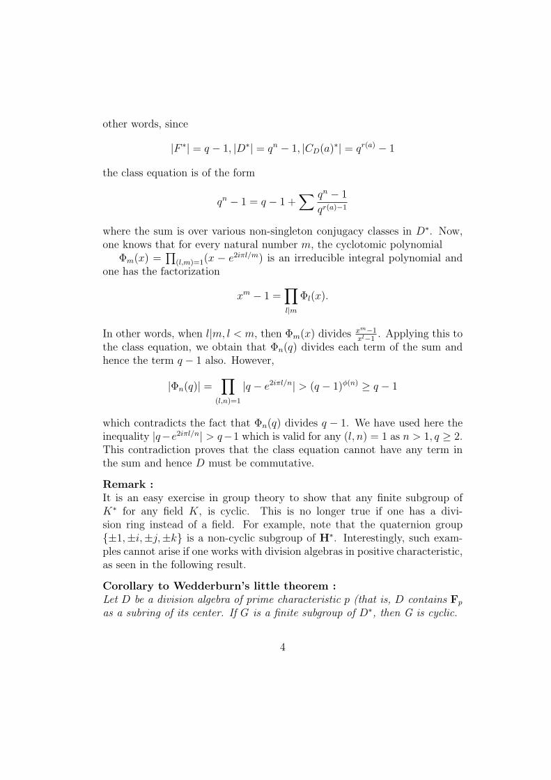
other words, since

|F ∗| = q − 1, |D∗| = qn − 1, |CD(a)∗| = qr(a) − 1

the class equation is of the form

qn − 1 = q − 1 +∑ qn − 1

qr(a)−1

where the sum is over various non-singleton conjugacy classes in D∗. Now,one knows that for every natural number m, the cyclotomic polynomial

Φm(x) =∏

(l,m)=1(x − e2iπl/m) is an irreducible integral polynomial andone has the factorization

xm − 1 =∏

l|mΦl(x).

In other words, when l|m, l < m, then Φm(x) divides xm−1xl−1

. Applying this tothe class equation, we obtain that Φn(q) divides each term of the sum andhence the term q − 1 also. However,

|Φn(q)| =∏

(l,n)=1

|q − e2iπl/n| > (q − 1)φ(n) ≥ q − 1

which contradicts the fact that Φn(q) divides q − 1. We have used here theinequality |q−e2iπl/n| > q−1 which is valid for any (l, n) = 1 as n > 1, q ≥ 2.This contradiction proves that the class equation cannot have any term inthe sum and hence D must be commutative.

Remark :It is an easy exercise in group theory to show that any finite subgroup ofK∗ for any field K, is cyclic. This is no longer true if one has a divi-sion ring instead of a field. For example, note that the quaternion group±1,±i,±j,±k is a non-cyclic subgroup of H∗. Interestingly, such exam-ples cannot arise if one works with division algebras in positive characteristic,as seen in the following result.

Corollary to Wedderburn’s little theorem :Let D be a division algebra of prime characteristic p (that is, D contains Fp

as a subring of its center. If G is a finite subgroup of D∗, then G is cyclic.

4

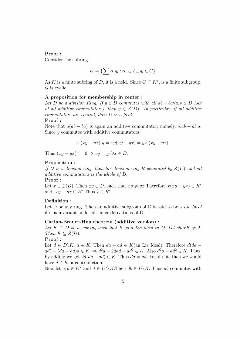
Proof :Consider the subring

K = ∑

αigi : αi ∈ Fp, gi ∈ G.

As K is a finite subring of D, it is a field. Since G ⊆ K∗, is a finite subgroup.G is cyclic.

A proposition for membership in center :Let D be a division Ring. If y ∈ D commutes with all ab− ba∀a, b ∈ D (setof all additive commutators), then y ∈ Z(D). In particular, if all additivecommutators are central, then D is a field.Proof :Note that a(ab − ba) is again an additive commutator, namely, a.ab − ab.a.Since y commutes with additive commutators

x.(xy − yx).y = xy(xy − yx) = yx.(xy − yx).

Thus (xy − yx)2 = 0 ⇒ xy = yx∀x ∈ D.

Proposition :If D is a division ring, then the division ring R generated by Z(D) and alladditive commutators is the whole of D.Proof :Let x ∈ Z(D). Then ∃y ∈ D, such that xy 6= yx.Therefore x(xy − yx) ∈ R∗

and xy − yx ∈ R∗.Thus x ∈ R∗.

Definition :Let D be any ring. Then an additive subgroup of D is said to be a Lie Idealif it is invariant under all inner derivations of D.

Cartan-Brauer-Hua theorem (additive version) :Let K ⊂ D be a subring such that K is a Lie ideal in D. Let charK 6= 2.Then K ⊆ Z(D).Proof :Let d ∈ D\K, a ∈ K. Then da − ad ∈ K(an Lie Ideal). Therefore d(da −ad)− (da− ad)d ∈ K. ⇒ d2a− 2dad + ad2 ∈ K. Also d2a− ad2 ∈ K. Thus,by adding we get 2d(da− ad) ∈ K. Thus da = ad. For if not, then we wouldhave d ∈ K, a contradiction.Now let a, b ∈ K∗ and d ∈ D∗\K.Then db ∈ D\K. Thus db commutes with

5

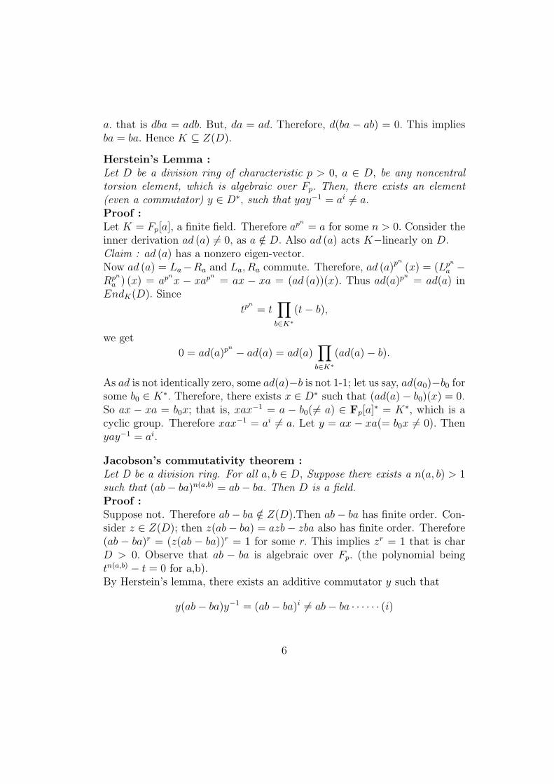
a. that is dba = adb. But, da = ad. Therefore, d(ba − ab) = 0. This impliesba = ba. Hence K ⊆ Z(D).

Herstein’s Lemma :Let D be a division ring of characteristic p > 0, a ∈ D, be any noncentraltorsion element, which is algebraic over Fp. Then, there exists an element(even a commutator) y ∈ D∗, such that yay−1 = ai 6= a.Proof :Let K = Fp[a], a finite field. Therefore apn

= a for some n > 0. Consider theinner derivation ad (a) 6= 0, as a /∈ D. Also ad (a) acts K−linearly on D.Claim : ad (a) has a nonzero eigen-vector.Now ad (a) = La−Ra and La, Ra commute. Therefore, ad (a)pn

(x) = (Lpn

a −Rpn

a ) (x) = apnx − xapn

= ax − xa = (ad (a))(x). Thus ad(a)pn= ad(a) in

EndK(D). Since

tpn

= t∏

b∈K∗(t− b),

we get

0 = ad(a)pn − ad(a) = ad(a)∏

b∈K∗(ad(a)− b).

As ad is not identically zero, some ad(a)−b is not 1-1; let us say, ad(a0)−b0 forsome b0 ∈ K∗. Therefore, there exists x ∈ D∗ such that (ad(a)− b0)(x) = 0.So ax − xa = b0x; that is, xax−1 = a − b0(6= a) ∈ Fp[a]∗ = K∗, which is acyclic group. Therefore xax−1 = ai 6= a. Let y = ax− xa(= b0x 6= 0). Thenyay−1 = ai.

Jacobson’s commutativity theorem :Let D be a division ring. For all a, b ∈ D, Suppose there exists a n(a, b) > 1such that (ab− ba)n(a,b) = ab− ba. Then D is a field.Proof :Suppose not. Therefore ab− ba /∈ Z(D).Then ab− ba has finite order. Con-sider z ∈ Z(D); then z(ab− ba) = azb− zba also has finite order. Therefore(ab − ba)r = (z(ab − ba))r = 1 for some r. This implies zr = 1 that is charD > 0. Observe that ab − ba is algebraic over Fp. (the polynomial beingtn(a,b) − t = 0 for a,b).By Herstein’s lemma, there exists an additive commutator y such that

y(ab− ba)y−1 = (ab− ba)i 6= ab− ba · · · · · · (i)

6

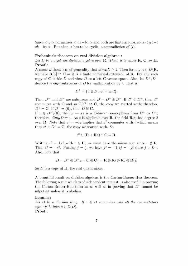
Since < y > normalizes < ab− ba > and both are finite groups, so is < y ><ab− ba > . But then it has to be cyclic, a contradiction of (i).

Frobenius’s theorem on real division algebras :Let D be a algebraic division algebra over R. Then, it is either R, C ,or H.Proof :Assume without loss of generality that dimRD ≥ 2. Then for any α ∈ D\R,we have R[α] ∼= C as it is a finite nontrivial extension of R. Fix any suchcopy of C inside D and view D as a left C-vector space. Also, let D+, D−

denote the eigensubspaces of D for multiplication by i. That is,

D± = d ∈ D : di = ±id.

Then D+ and D− are subspaces and D = D+ ⊕ D−. If d+ ∈ D+, then d+

commutes with C and so C[d+] ∼= C, the copy we started with; thereforeD+ = C. If D− = 0, then D ∼= C.If z ∈ D−\0, then x → xz is a C-linear isomorphism from D+ to D−;therefore, dimRD = 4. As z is algebraic over R, the field R[z] has degree 2over R. Note that zi = −iz implies that z2 commutes with i which meansthat z2 ∈ D+ = C, the copy we started with. So

z2 ∈ (R + Rz) ∩C = R.

Writing z2 = ±r2 with r ∈ R, we must have the minus sign since z 6∈ R.Thus z2 = −r2. Putting j = z

r, we have j2 = −1, ij = −ji since j ∈ D−.

Also, note that

D = D+ ⊕D+z = C⊕Cj = R⊕Ri⊕Rj ⊕Rij.

So D is a copy of H, the real quaternions.

A beautiful result on division algebras is the Cartan-Brauer-Hua theorem.The following result which is of independent interest, is also useful in provingthe Cartan-Brauer-Hua theorem as well as in proving that D∗ cannot benilpotent unless it is abelian.

Lemma :Let D be a division Ring. If a ∈ D commutes with all the commutatorsxyx−1y−1, then a ∈ Z(D).Proof :

7

Suppose a /∈ Z(D). Then there exists an element b such that ab 6= ba. Thenb 6= 0,−1 and so b−1, (b + 1)−1 exist and we have

1− aba−1b−1 = 1 + aba−1 − aba−1 − aba−1b−1

= a(b + 1)a−1 − aba−1b−1(b + 1)

= (a(b + 1)a−1(b + 1)−1 − aba−1b−1)(b + 1).

Now as a commutes with all commutators, and thus, it commutes with theleft hand side as well as with the two terms within the first bracket on theright hand side. Therefore a commutes with b + 1, and hence with b itself,which is a contradiction.

Cartan-Brauer-Hua theorem (multiplicative version) :Let A ⊆ D be a division subring stable under all inner conjugations of D.Then A = D or A ⊆ Z(D).Proof :Assume A 6= D. Let a ∈ A∗, b ∈ D\A. Using the identity in the lemma wehave a−1 − ba−1b−1 = ((b + 1)a−1(b + 1)−1 − ba−1b−1)(b + 1). Since the lefthand side is in A and (b+1)a−1(b+1)−1− ba−1b−1 ∈ A, and since b+1 6∈ A,we have that the left hand side must be 0. Thus ab = ba. Let now a′ ∈ A.Then a′b ∈ D\A.So a.a′b = a′b.a = a′.ba = a′.ab; that is, aa′ = a′a. Therefore A ⊆ Z(D).

Corollary :(i) Let D be a division ring and assume d ∈ D\Z(D). Then D is generatedby the conjugates of d.(ii)If D is a noncommutative division ring, then it is generated as a divisionring by all xyx−1y−1.

Theorem (nilpotence implies abelian) :Let D be a division ring and

1 ⊆ G1 ⊆ G2 ⊆ · · ·

be the upper central series of D∗; that is,

G1 = Z(D∗), Gi+1/Gi = Z(D∗/Gi), · · ·

ThenG1 = G2 = · · · · · ·

8

Hence D∗ is nilpotent if and only if D is a field.Proof :We shall use the Carter-Brauer-Hua theorem. Let a ∈ G2\G1. So axa−1x−1 ∈G1∀x ∈ D∗. So a /∈ G1 = Z(D). Therefore there exists b ∈ D∗ such thatab 6= ba. From the identity

1− aba−1b−1 = a(b + 1)a−1(b + 1)−1 − aba−1b−1(b + 1)

we have(a(b + 1)a−1(b + 1)−1 − aba−1b−1)(b + 1) ∈ Z(D).

Since Z(D) is a field, we have b + 1 ∈ Z(D), which is a contradiction.

Remarks and definitions :Let F = Z(D) be the center of a division ring D. If f(t) ∈ F [t], andif a ∈ D is a root of f, then so is any conjugate of a. Also note that ifa ∈ D is algebraic over F (that is, it satisfies a nonzero polynomial over F ),then so are all its conjugates and they have the same minimum polynomialover F , which is called the minimum polynomial of the conjugacy class. Infact, if D is algebraic over F , and a ∈ D, then any other root of the minimalpolynomial of a must be conjugate to a in D ! This follows from the followingvery important and widely used result :

Skolem-Noether theorem :Let A be a central simple algebra over K. Let B be a simple K algebra. Letσ, τ : B → A be two algebra homomorphisms. Then there exists an innerautomorphism Int(a) of A such that τ = Int(a) σ.Proof :Consider the case A = End(V ) for a K vector space V. Then V is alsoa A−module. Via σ and τ we can view V as a B module in two ways.Call them Vσ and Vτ . Since all B simple modules have to be isomorphic bySchur’s lemma, there exists a B-isomorphism f : Vτ → Vσ that is ∀b ∈ B, x ∈V, f(τ(b)x) = σ(b)(f(x)). Hence τ(b) = f−1σ(b)f. Since f ∈ A, we have theresult in this case.In the general case we consider B⊗K Ao for B and A⊗K Aop for A where Aop

denotes the opposite algebra of A. Consider σ⊗ id, τ ⊗ id from B ⊗K Aop →A⊗K Aop ∼= EndK(A).The last isomorphism is seen as follows. For a ∈ A, b ∈ Aop, the map φ :A → A given by φ(x) = axb is an endomorphism of the K vector space A.

9

Now the map a⊗ b → φ is the required isomorphism.By the first case there exists an α ∈ A⊗K Aop such that

(σ ⊗ id)(x) = α(τ ⊗ id)(x)α−1∀x ∈ B ⊗ Aop · · · (i)

Hence α ∈ CA⊗Aop(1⊗ Aop) = A⊗ 1.Writing α = a⊗1 and applying (i) to x = c⊗1, we get σ(c) = aτ(c)a−1. Notethat the first case applies because B ⊗ Ao is simple for the general reasonthat whenever X is a central simple algebra and Y is simple over K, thenX ⊗K Y is simple.

10

§ Polynomials over division algebras

Over a field K, a non-zero polynomial f can have at the most deg f roots;this is easy to see using the remainder theorem. However, already over H,we see that i, j, k etc. are all roots of the polynomial t2 + 1. Moreover,our familiar intuitions from equations over fields often fails in many otherways. For example, over a field, a polynomial with a factor of the form t− aevidently vanishes when evaluated at a. However, look at the polynomial(t − i)(t − j) = t2 − (i + j)t + ij over the Hamilton quaternion divisionalgebra H. The value at i is

i2 − (i + j)i + ij = ij − ji 6= 0!

Note however that the value at j is 0. A careful look at this aspect revealsthe following. In the above, we are writing polynomials in the form c0 +c1t + c2t

2 + · · · + cntn with the constants ci on the left and the powers ofthe variable t on the right. When we specialize a value of t, obviously thevalue depends on whether the variable has appeared to the left or to theright. As we shall see, if we write polynomials in the above familiar formwith the coefficients to the left, various facts like remainder theorem holdgood when we look at ‘right’ remainders. If we consider a polynomial ofthe form g(t)(t − a) (with the same convention of writing coefficients onthe left), it will turn out that the polynomial vanishes when evaluated ata. Similarly, if we were to write polynomials with the coefficients on theright, we would have a ‘left’ remainder theorem etc. In this section, westudy polynomial equations over noncommutative division rings and describethe various points of departure from equations over fields. The results aresurprising and interesting. Without further ado, let us discuss these aspectsnow.

Firstly, here is a curious characterization of division rings using linear equa-tions. Note that a general linear equation over a noncommutative ring isof the form

∑ri=1 aixbi = c. The equation which has been studied is the

equation of the form ax− xb = c. The following result characterizes divisionrings in terms of solutions of this type of equations.

Let R be a ring with unity. Assume that the equation ax−xb = c is solvable inx whenever a 6= b. Then R is a division ring. Further, if each such equation

11

has a unique solution, then R is a field.Proof :For the first statement, consider a ∈ R, a 6= 0, b = 0 and c = 1. Then theequation reads ax = 1. Let x = a1 be a solution Then aa1 = 1. Note thata1 6= 0 and so we also have a2 such that a1a2 = 1. Thus a = a(a1a2) =(aa1)a2 = a2. Thus each a ∈ R is invertible and hence R is a division ring.For the second statement, let us suppose R to be a noncommutative ringwhich admits a solution for each equation of the form ax − xb = c witha 6= b. If ab 6= ba for some a, b, then the equation abx − xba = 0 has twodifferent solutions 0 and a. So the above type of equations over R can haveunique solutions only if R is commutative.

Open question :Is there a division ring which is not a field and admits solutions for everyequation of the form ax− xb = c with a 6= b ?

Let R be any ring and D be a division ring contained in R. If f(t) =∑

aiti ∈

R[t], we define the value f(r) :=∑

airi. We call r ∈ R a right root of

f(t) =∑

aiti, if f(r) = 0.

Note that∑

i airi may not be equal to

∑i r

iai.In particular, if f(t) = g(t)h(t), then we may not have f(r) = g(r)h(r); thatis, the ‘evaluation map’ may not be a homomorphism. However, sticking tothis ‘evaluation’ map, an easy observation is the right factor theorem statednext. Following that is a key lemma which tells us what one can say abouta root of g(t)h(t) which is not a root of h(t).

Right factor theorem :Let R be any ring and r ∈ R is a root of f(t) if and only if t − r is a rightdivisor of f(t) in R[t]. The set of polynomials having r as a root is the leftideal R[t](t− r).

Lemma :Let f(t) = g(t)h(t) ∈ D[t]. If d ∈ D is such that h(d) = a 6= 0, thenf(d) = g(ada−1)h(d). Consequently, if d is a root of f but not a root of h,then ada−1 is a root of g.Proof:Let g(t) =

∑mi=1 bit

i. Then f(t) =∑m

i=1 bih(t)ti. So

f(d) =m∑

i=1

bih(d)di =m∑

i=1

biadi =m∑

i=1

biadia−1a =m∑

i=1

bi(ada−1)ia = g(ada−1)h(d).

12

Corollary :If f(t) = (t − a1)(t − a2) · · · (t − an) where ai ∈ D. Then every root of f isconjugate to one of the ai’s.

As we observed earlier, x2 + 1 = 0 has infinite roots over the division ring H(division ring of real quaternions). The following result is a generalisation ofthe familiar result that over a field, a polynomial has at the most its degreenumber of roots :

Theorem (Gordon-Motzkin) :Let D be a division ring. If f(t) ∈ D[t], then all its roots lie in at most nconjugacy classes where deg f = n.Proof:We proceed by induction on n. For n = 1 it is obvious. Suppose n ≥ 2 andlet r be a root of f.Then by the proposition above f(t) = g(t)(t−r) for someg(t) ∈ D[t] of degree n− 1. If s 6= r is another root of f , then by the lemma,s is conjugate to a root of g which in turn lies in one of the n− 1 conjugacyclasses by the induction hypothesis. Thus by induction, we have the result.

Lemma :Let A be an algebraic conjugacy class in D(over F ) with minimum polynomialf(t) ∈ F [t]. If a polynomial h(t) ∈ D[t]\0 vanishes identically on A, thendeg h ≥ deg f.Proof :Suppose not. Pick a polynomial h(t) = tm+a1t

m−1+· · ·+am such that h(A) =0 and m < deg f. Since h(t) 6∈ F [t], some ai 6∈ F. Therefore there exists anelement b ∈ D∗ so that bai 6= aib. Clearly now am + a1a

m−1 + · · · + am = 0∀a ∈ A. Conjugating by b, we have

(bab−1)m + (ba1b−1)(bab−1)m−1 + · · ·+ (bamb−1) = 0 ∀a ∈ A · · · (I)

But since bab−1 ∈ A,

(bab−1)m + a1(bab−1)m−1 + · · ·+ am = 0 ∀a ∈ A · · · (II)

From (I) and (II), we get that∑

(baib−1 − ai)t

m−i vanishes on A; this con-tradicts the choice of m and proves the lemma.

Corollary :If h(t) ∈ D[t] vanishes on A if and only if h(t) ∈ D[t]f(t).

13

Proof :If f(a) = 0∀a ∈ A, then f(t) ∈ D[t](t− a). If h(t) ∈ D[t]f(t), clearly h(t) ∈D[t](t−a) and therefore h(A) = 0. Conversely, if h(A) = 0, h(t) 6= 0, then bydivision algorithm, h(t) = g(t)f(t)+r(t), with deg r(t) < deg f(t), where f(t)is the minimum polynomial of the conjugacy class A. Since h(A) = f(A) = 0,we have r(t) = 0. Thus, from the lemma above we have deg h > deg f. Thush(t) = g(t)f(t) ⇒ h(t) ∈ D[t]f(t).

Corollary :Let D be an infinite division ring. Then if h(t) ∈ D[t] is such that h(d) =0∀d ∈ D, then h(t) = 0, the zero polynomial.Proof :Suppose not. Pick a monic polynomial h of least degree such that h(d) = 0∀d ∈ D. Let h(t) = tm + a1t

m−1 + · · · + am. We get that all ai ∈ Z(D) = F(similar to the argument used in the lemma). Therefore, h(t) ∈ F [t]. Sinceh(F ) = 0, F is finite. Now h(D) = 0 ⇒ D is algebraic over F , and so D iscommutative. This is a contradiction.

Theorem(Dickson) :Let a, b ∈ D be algebraic over F. Then a is conjugate to b in D if and only ifthey have the same minimum polynomial.Proof :Clearly, if a, b are conjugates, then they have the same minimum polynomial.Conversely, suppose f is the common minimum polynomial for a and b.Regarding f as an element of F (a)[t], f(t) = g(t)(t− a) = (t− a)g(t) by theremainder theorem over fields. Since deg g < deg f and f is the minimumpolynomial of b, by the lemma there exists some conjugate xbx−1 of b in Dsuch that g(xbx−1) 6= 0. But f(t) ∈ F [t] is the minimum polynomial of b, andso f(aba−1) = 0 since f(xbx−1) = 0, g(xbx−1) 6= 0, therefore some conjugateof xbx−1 is a zero of t−a by the lemma prior to the Gordon-Motzkin theorem.Thus a is conjugate to b.

Theorem (Wedderburn) :Let A be a conjugacy class which is algebraic over F. Let f denote its mini-mum polynomial over F and suppose n = deg f. Then there exist a1, a2, · · · , an ∈A such that f(t) = (t− an) · · · (t− a1). Moreover a1 ∈ A can be chosen arbi-trarily. Further the decomposition of f can be cyclically permuted.Proof :Let a1 ∈ A be arbitrary. Since f(a1) = 0,Therefore f(t) = g(t)(t − a1)

14

for some g(t). If A = a1, then a1 ∈ F and therefore f(t) = (t − a1).If A 6= a1, there exists a conjugate a′2 of a1 such that a′2 6= a1. Sincef(a′2) = 0. Therefore g vanishes at some conjugate a2 of a′2. Therefore wecan write g(t) = g2(t)(t − a2). that is f(t) = g2(t)(t − a2)(t − a1). Pro-ceeding this way, we get f(t) = gr(t)(t − ar) · · · (t − a1) with r maximumpossible. This implies by the above discussion that a1, · · · , ar = A. Sinceh(t) := (t−ar) · · · (t−a1) vanishes identically on A, we have h(t) ∈ D[t]f(t).That is, deg h ≥ deg f. But f(t) = gr(t)h(t). Therefore f(t) = h(t). Finally,cyclic permutations are possible because a factorization of a polynomial inF [t] into two factors in D[t] is necessarily commutative; that is, if α ∈ F [t],α = β1(t)β2(t), βi ∈ D[t], then β1(t)β2(t) = β2(t)β1(t)).

Corollary :With the same notations as above, if f(t) = tn +d1t

n−1 + · · ·+dn ∈ F [t], thend1 is a sum of the elements of A and (−1)ndn is the product of the elementsof A.

Remarks :From the above theorem we note that there are infinitely many factorizations.This is because, from the above theorem, we saw that a1 was arbitrary.We know that A is infinite unless A = a1, a1 ∈ F. The next theoremdeals further on the above theme for polynomial equations; it shows thatpolynomials with at least 2 conjugate zeroes has infinitely many.

Theorem (Gordon-Motzkin) :Let D be a division ring and f(t) =

∑ni=0 ait

i ∈ D[t]. Let A be a conjugacyclass in D. Assume that f has atleast two zeroes in A. Then f has infinitelymany zeroes in A. In particular, for f = 0, this means that |A| ≥ 2 ⇒ |A| isinfinite.Proof :Fix any a ∈ A. If some dad−1 is a zero of f, then

∑aidai = 0. So, we must

look for d ∈ D∗ such that∑

aidai = 0. Define Φ : D → D; such that Φ(d) =∑aidai. Then Φ(dz) = Φ(d)z∀z ∈ CD(a). Therefore the centralizer CD(a) of

a acts on ker Φ on the right. We have a map θ : D∗∩ker Φ → zeroes of f in A.θ(d) = dad−1. Note θ(d) = θ(d′) if and only if d ∈ d′.CD(a). Thus the set ofzeroes of f in A is in bijection with ker Φ\0/CD(a), the projective space ofthe right CD(a) vector space ker Φ. We are given that ker Φ has dim ≥ 2 overCD(a). Thus, the corresponding projective space ker Φ\0/CD(a) is infinite,since CD(a) is infinite (because D is not commutative since |A| ≥ 2).

15

Corollary :If f(t) ∈ D[t] has degree n and Γ be the set of roots in D, then either |Γ| ≤ nor Γ is infinite.Proof :Suppose |Γ| > n and let a1, · · · , an+1 ∈ Γ be distinct. Since the zero of f liein at most n conjugacy classes, atleast two of the ai’s are conjugate. By theabove theorem, the corresponding conjugacy class intersects Γ in an infiniteset.

Remarks :Over fields, we know that given n distinct points c1, · · · , cn, there exists aunique polynomial of degree ≤ n vanishing at c1, · · · , cn; namely, the poly-nomial (t − c1) · · · (t − cn). The analogue for division rings is the followingtheorem.

Theorem(Bray-Whaples) :Let D be a division ring and let c1, · · · , cn be pairwise nonconjugate elementsof D. Then there exists a unique polynomial f(t) ∈ D[t] such that f(ci) = 0∀i.Further, this polynomial necessarily satisfies :(a) c1, · · · , cn are its only zeroes,(b) if h(t) ∈ D[t] vanishes at all the ci ’s, then h(t) ∈ D[t]f(t).Proof :The uniqueness is clear. This is because the difference of two such polyno-mials would be a polynomial vanishing at n points in n distinct conjugacyclasses while having degree ≤ n − 1, which is a contradiction. To see theexistence, we proceed by induction on n.For n = 1, f(t) = t− c1 clearly. For n = 2, choose d2 so that (t− d2)(t− c1)vanishes at c2 (this clearly means d2 = (c2− c1)c2(c2− c1)

−1). Proceeding inthis way, we can get clearly f(t)in the form (t− dn) · · · (t− d2)(t− c1) wheredi is the conjugate of ci. This proves the existence of f also.To prove (b), we divide h by f and write h(t) = q(t)f(t) + r(t). Sinceh(ci) = 0, and (q(t)f(t))(ci) = 0, r(ci) = 0. And deg r < n and r van-ishes at points from n distinct conjugacy classes. Thus r(t) ≡ 0.To prove (a), we again proceed by induction on n. For n = 1, it is clear.Assume the result for all m < n. Write fn(t) = (t − d)fm(t). where fn(t) isthe unique polynomial vanishing at c1, · · · , cn and fm(t) is the one vanishingat c1, · · · , cn−1. Observe that d is the conjugate of cn. Suppose fn(c) = 0 forsome c ∈ D. If fm(c) = 0, then c must be one among c1, · · · , cn−1 by induc-

16

tion hypothesis. Therefore, assume fm(c) 6= 0. Then c is a conjugate of dand therefore of cn.We claim that d = cn. Suppose not. Consider the polynomial g(t) =(t − e)(t − cn) where e is chosen so that g(c) = 0 where e is chosen sothat g(c) = 0. Indeed e = (c − cn)e(c − cn)−1. Divide fn by g and writefn(t) = q(t)g(t) + r(t), where deg r < deg g = 2. Since fn vanishes at cand cn and since (q(t)g(t)) vanishes at c and cn, therefore r(t) vanishes atc and cn. But deg r ≤ 1. Thus, the only possibility is r ≡ 0 (as c 6= cn).Therefore fn(t) = q(t)g(t). Therefore deg q ≤ n−2. But g does not vanish atc1, · · · , cn−1, as any zero of g is conjugate of cn. Now q vanishes at conjugatesof c1, · · · , cn−1, which is a contradiction since deg q ≤ n− 2. Thus c = cn.

Analogous to fields being algebraically closed, there is a notion of a divisionring being right-algebraically-closed. D is defined to be so if every nonconstantpolynomial f in one variable over D has a right root in D. A theorem of Baersays that the only noncommutative division ring which is right algebraicallyclosed is necessarily the ring of quaternions over a real closed field. Recallthat a field is said to be real closed if (like in R) −1 is not a sum of squaresin it.

Lemma :Let D be any division ring with center F, and A be a conjugacy class of Dwhich has a quadratic minimum polynomial λ(t). If f(t) ∈ D[t] has two rootsin A, then f(t) ∈ D[t]λ(t) and f(A) = 0.

Proposition(Niven) :Take R to be a real closed field, and D = R ⊕ Ri ⊕ Rj ⊕ Rk be the ring ofquaternions over R. For 0 6= f(t) ∈ D[t], the following are equivalent:(i)f(t) has infinitely many roots in D.(ii) There exist a, b ∈ R with b 6= 0 such that f(a + ib) = 0 = f(a− ib).(iii) f has a right factor λ(t) which is an irreducible quadratic in R[t].If these three equivalent conditions hold for f then f vanishes on the conju-gacy class of a + bi.Proof :Assume (i) holds. Then f(t) has two roots in certain conjugacy class A. Theminimum polynomial λ(t) of A over R is an irreducible quadratic over R.By the above lemma, we have f(t) ∈ D[t]λ(t). Thus, being quadratic its tworoots are of the form a + bi and a− bi. This proves (ii) holds.Now, assume (iii). Let c be the root of λ(t) in R(i). c has infinitely many

17

conjugates in D. All these are roots of λ(t) and hence of f(t). This proves(iii) from (i).Now (ii) ⇒ (iii) is easily deduced from the remainder theorem.

Here is a beautiful result on polynomials over division rings over real closedfields.

Proposition :Let D,R be as above, and let f(t) =

∑ni=0 ait

i, where a0 ∈ D\R, anda1, · · · , an ∈ R. Then f has at most n roots in D.Proof :Let α be any root of f. Then α commute with

∑aiα

i = −a0. Thereforeα ∈ CD(R(α0)). But in this case R(α0) is a maximal subfield of D and there-fore CD(R(α0)) = R(α0). Thus α ∈ R(α0). Thus every root is in the fieldR(α0). Since f has at most n roots in a field, the proposition is proved.

Corollary (Niven) :For a ∈ D \ R, the equation tn = a has exactly n solutions in D and all ofthem lie in R(α0).

18

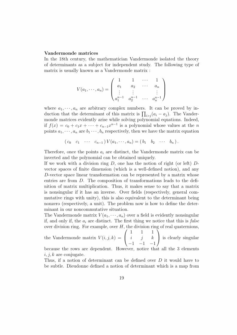
Vandermonde matricesIn the 18th century, the mathematician Vandermonde isolated the theoryof determinants as a subject for independent study. The following type ofmatrix is usually known as a Vandermonde matrix :

V (a1, · · · , an) =

1 1 · · · 1a1 a2 · · · an...

......

an−11 an−1

2 · · · an−1n

where a1, · · · , an are arbitrary complex numbers. It can be proved by in-duction that the determinant of this matrix is

∏i>j(ai − aj). The Vander-

monde matrices evidently arise while solving polynomial equations. Indeed,if f(x) = c0 + c1x + · · · + cn−1x

n−1 is a polynomial whose values at the npoints a1, · · · , an are b1 · · · , bn respectively, then we have the matrix equation

( c0 c1 · · · cn−1 ) V (a1, · · · , an) = ( b1 b2 · · · bn ) .

Therefore, once the points ai are distinct, the Vandermonde matrix can beinverted and the polynomial can be obtained uniquely.If we work with a division ring D, one has the notion of right (or left) D-vector spaces of finite dimension (which is a well-defined notion), and anyD-vector space linear transformation can be represented by a matrix whoseentries are from D. The composition of transformations leads to the defi-nition of matrix multiplication. Thus, it makes sense to say that a matrixis nonsingular if it has an inverse. Over fields (respectively, general com-mutative rings with unity), this is also equivalent to the determinant beingnonzero (respectively, a unit). The problem now is how to define the deter-minant in our noncommutative situation.The Vandermonde matrix V (a1, · · · , an) over a field is evidently nonsingularif, and only if, the ai are distinct. The first thing we notice that this is falseover division ring. For example, over H, the division ring of real quaternions,

the Vandermonde matrix V (i, j, k) =

1 1 1i j k−1 −1 −1

is clearly singular

because the rows are dependent. However, notice that all the 3 elementsi, j, k are conjugate.Thus, if a notion of determinant can be defined over D it would have tobe subtle. Dieudonne defined a notion of determinant which is a map from

19

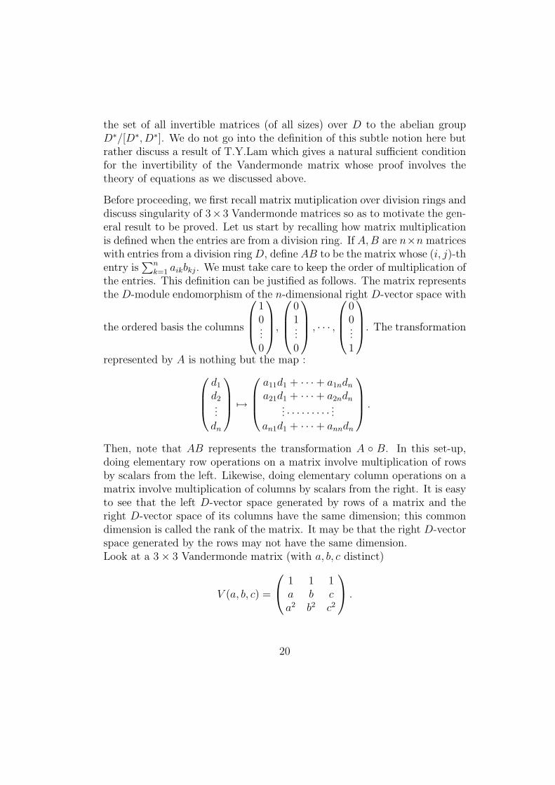
the set of all invertible matrices (of all sizes) over D to the abelian groupD∗/[D∗, D∗]. We do not go into the definition of this subtle notion here butrather discuss a result of T.Y.Lam which gives a natural sufficient conditionfor the invertibility of the Vandermonde matrix whose proof involves thetheory of equations as we discussed above.

Before proceeding, we first recall matrix mutiplication over division rings anddiscuss singularity of 3× 3 Vandermonde matrices so as to motivate the gen-eral result to be proved. Let us start by recalling how matrix multiplicationis defined when the entries are from a division ring. If A, B are n×n matriceswith entries from a division ring D, define AB to be the matrix whose (i, j)-thentry is

∑nk=1 aikbkj. We must take care to keep the order of multiplication of

the entries. This definition can be justified as follows. The matrix representsthe D-module endomorphism of the n-dimensional right D-vector space with

the ordered basis the columns

10...0

,

01...0

, · · · ,

00...1

. The transformation

represented by A is nothing but the map :

d1

d2...

dn

7→

a11d1 + · · ·+ a1ndn

a21d1 + · · ·+ a2ndn... · · · · · · · · · ...

an1d1 + · · ·+ anndn

.

Then, note that AB represents the transformation A B. In this set-up,doing elementary row operations on a matrix involve multiplication of rowsby scalars from the left. Likewise, doing elementary column operations on amatrix involve multiplication of columns by scalars from the right. It is easyto see that the left D-vector space generated by rows of a matrix and theright D-vector space of its columns have the same dimension; this commondimension is called the rank of the matrix. It may be that the right D-vectorspace generated by the rows may not have the same dimension.Look at a 3× 3 Vandermonde matrix (with a, b, c distinct)

V (a, b, c) =

1 1 1a b ca2 b2 c2

.

20

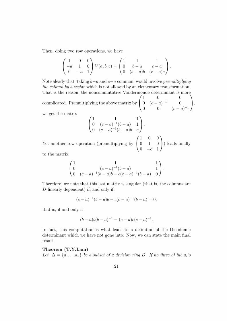
Then, doing two row operations, we have

1 0 0−a 1 00 −a 1

V (a, b, c) =

1 1 10 b− a c− a0 (b− a)b (c− a)c

.

Note aleady that ‘taking b−a and c−a common’ would involve premultiplyingthe column by a scalar which is not allowed by an elementary transformation.That is the reason, the noncommutative Vandermonde determinant is more

complicated. Premultiplying the above matrix by

1 0 00 (c− a)−1 00 0 (c− a)−1

,

we get the matrix

1 1 10 (c− a)−1(b− a) 10 (c− a)−1(b− a)b c

.

Yet another row operation (premultiplying by

1 0 00 1 00 −c 1

) leads finally

to the matrix

1 1 10 (c− a)−1(b− a) 10 (c− a)−1(b− a)b− c(c− a)−1(b− a) 0

.

Therefore, we note that this last matrix is singular (that is, the columns areD-linearly dependent) if, and only if,

(c− a)−1(b− a)b− c(c− a)−1(b− a) = 0;

that is, if and only if

(b− a)b(b− a)−1 = (c− a)c(c− a)−1.

In fact, this computation is what leads to a definition of the Dieudonnedeterminant which we have not gone into. Now, we can state the main finalresult.

Theorem (T.Y.Lam)Let ∆ = a1, ....an be a subset of a division ring D. If no three of the ai’s

21

lie in a single conjugacy class, then the Vandermonde matrix Vn(a1, ....an) isinvertible.

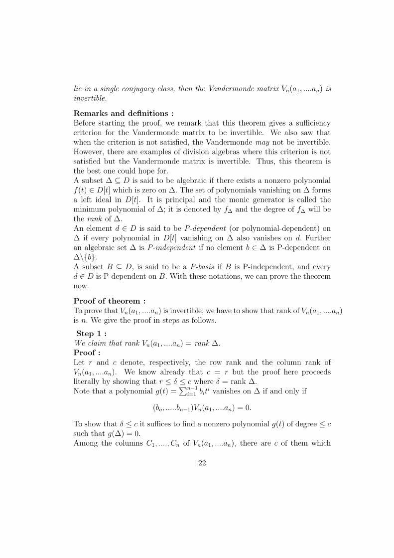
Remarks and definitions :Before starting the proof, we remark that this theorem gives a sufficiencycriterion for the Vandermonde matrix to be invertible. We also saw thatwhen the criterion is not satisfied, the Vandermonde may not be invertible.However, there are examples of division algebras where this criterion is notsatisfied but the Vandermonde matrix is invertible. Thus, this theorem isthe best one could hope for.A subset ∆ ⊆ D is said to be algebraic if there exists a nonzero polynomialf(t) ∈ D[t] which is zero on ∆. The set of polynomials vanishing on ∆ formsa left ideal in D[t]. It is principal and the monic generator is called theminimum polynomial of ∆; it is denoted by f∆ and the degree of f∆ will bethe rank of ∆.An element d ∈ D is said to be P-dependent (or polynomial-dependent) on∆ if every polynomial in D[t] vanishing on ∆ also vanishes on d. Furtheran algebraic set ∆ is P-independent if no element b ∈ ∆ is P-dependent on∆\b.A subset B ⊆ D, is said to be a P-basis if B is P-independent, and everyd ∈ D is P-dependent on B. With these notations, we can prove the theoremnow.

Proof of theorem :To prove that Vn(a1, ....an) is invertible, we have to show that rank of Vn(a1, ....an)is n. We give the proof in steps as follows.

Step 1 :We claim that rank Vn(a1, ....an) = rank ∆.Proof :Let r and c denote, respectively, the row rank and the column rank ofVn(a1, ....an). We know already that c = r but the proof here proceedsliterally by showing that r ≤ δ ≤ c where δ = rank ∆.Note that a polynomial g(t) =

∑n−1i=1 bit

i vanishes on ∆ if and only if

(bo, .....bn−1)Vn(a1, ....an) = 0.

To show that δ ≤ c it suffices to find a nonzero polynomial g(t) of degree ≤ csuch that g(∆) = 0.Among the columns C1, ...., Cn of Vn(a1, ....an), there are c of them which

22

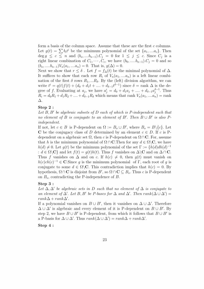
form a basis of the column space. Assume that these are the first c columns.Let g(t) =

∑bit

i be the minimum polynomial of the set a1, ....ac. Thendeg g ≤ c ≤ n and (bo, ....bn−1).Cj = 0 for 1 ≤ j ≤ c. Since Cj is aright linear combination of C1, · · · , Cc, we have (b0, .....bn−1).Cj = 0 and so(bo, .....bn−1)Vn(a1, ....an) = 0. That is, g(∆) = 0.Next we show that r ≤ δ . Let f = f∆(t) be the minimal polynomial of ∆.It suffices to show that each row Ri of Vn(a1, ....an) is a left linear combi-nation of the first δ rows R1, ...Rδ. By the (left) division algorithm, we canwrite ti = q(t)f(t) + (d0 + d1t + .... + dδ−1t

δ−1) since δ = rank ∆ is the de-gree of f. Evaluating at aj, we have ai

j = d0 + d1aj + .... + dδ−1aδ−1j . Thus

Ri = d0R1 + d1R2 + ....+ dδ−1Rδ which means that rank Vn(a1, ....an) = rank∆.

Step 2 :Let B, B′ be algebraic subsets of D each of which is P-independent such thatno element of B is conjugate to an element of B′. Then B ∪ B′ is also P-independent.If not, let c ∈ B is P-dependent on Ω := Bo ∪ B′, where Bo = B\c. LetC be the conjugacy class of D determined by an element c ∈ D. If c is P-dependent on a algebraic set Ω, then c is P-dependent on Ω∩C. For, assumethat h is the minimum polynomial of Ω∩C.Then for any d ∈ Ω\C, we haveh(d) 6= 0. Let g(t) be the minimum polynomial of the set Γ := h(d)dh(d)−1

: d ∈ Ω\C and let f(t) = g(t)h(t). Thus f vanishes on ∆\C and on ∆∩C.Thus f vanishes on ∆ and on c. If h(c) 6= 0, then g(t) must vanish onh(c)ch(c)−1 ∈ C.Since g is the minimum polynomial of Γ, each root of g isconjugate to some d ∈ Ω\C. This contradiction implies that h(c) = 0. Byhypothesis, Ω∩C is disjoint from B′, so Ω∩C ⊆ Bo. Thus c is P-dependenton Bo, contradicting the P-independence of B.

Step 3 :Let ∆, ∆′ be algebraic sets in D such that no element of ∆ is conjugate toan element of ∆′. Let B, B′ be P-bases for ∆ and ∆′. Then rank(∆ ∪∆′) =rank∆ + rank∆′.If a polynomial vanishes on B ∪ B′, then it vanishes on ∆ ∪ ∆′. Therefore∆ ∪ ∆′ is algebraic and every element of it is P-dependent on B ∪ B′. Bystep 2, we have B ∪ B′ is P-dependent, from which it follows that B ∪ B′ isa P-basis for ∆ ∪∆′. Thus rank(∆ ∪∆′) = rank∆ + rank∆′.

Step 4 :

23

Let ∆ be the algebraic set in D. Then rank∆ =∑

rank(∆ ∩ C), where Cranges over the finitely many conjugacy classes which intersects ∆. Furtherif |∆ ∩C| ≤ 2 for each C then |∆| < ∞ and ∆ is P-independent.The first statement is proved from step 3 and induction. If there exists onlyone conjugacy class which intersects ∆, then the statement immediately fol-lows. If there are two conjugacy classes which intersect ∆, then the statementfollows from step 3. Let the statement be true for n − 1 conjugacy classes.Suppose there exists n conjugacy classes which intersects ∆. Let the conju-gacy classes be Ci for 1 ≤ i ≤ n and let ∆i = ∆ ∩ Ci.Let ∆′ = ∪n−1

i=1 ∆i.Again, by step 3 we have rank(∆n−1 ∪∆′) = rank∆n−1 + rank∆′.Thus we have rank∆ =

∑ni−1 rank(∆i) =

∑ni−1 rank(∆ ∩Ci).

The second statement of step 4 follows from the first statement and the factthat no doubleton set is P-independent.

Let us see how the proof follows from these steps. Now since no three ai’sare in the same conjugacy class, the hypothesis of step 4 is fulfilled and wehave ∆ = a1, ....an is P-independent. Inductively we may assume thatrank(∆\a1) = n−1. Let f be the minimum polynomial of ∆ and g be theminimum polynomial of ∆\a1. Then f is a left multiple of g but f 6= g.Hence deg f ≥ 1 + deg g = n.On the other hand, deg f ≤ |∆| = n, hence rank ∆ = deg f = n.Since rank ∆ = n, it follows from step 1 that Vn(a1, · · · , an) is invertible.This completes the proof.

24