DNS Study on Motion around a Vortex Ring in Transitional ...Figure 8. The shape of a vortex ring and its vortex filaments in boundary layers 2. Maximum velocity around some vortex

http://www.uta.edu/math/preprint/

Technical Report 2015-05

DNS Study on Motion around a Vortex Ring in Transitional

Boundary Layers

Yiqian Wang Shuhyi Chern Chaoqun Liu

American Institute of Aeronautics and Astronautics

1

DNS Study on Motion around a Vortex Ring

in Transitional Boundary Layers

Yiqian Wang1, Shuhyi Chern

2, Chaoqun Liu

3

University of Texas at Arlington, Arlington, Texas 76019

Vortex rings are common in turbulent flows of liquids and gases. Therefore, considerable

attention has been paid to investigate their movement and deformation. However, researches

on the motion around vortex rings, especially in turbulent boundary layer, are relatively

rare. In this paper, the motion around a vortex ring in turbulent boundary layers is carefully

examined using the DNS results of a flat-plate boundary layer. Velocities, vorticities, vortex

filaments and pressure distribution are illustrated with iso-surfaces of λ2 representing the

vortices and vortex filaments. The toroidal motion of the vortices is also studied to show how

quick the vortex rotation is. It is found that there is substantial discrepancy between the

DNS results and time-averaged mathematical modeling like RANS or regular experiments

for the transitional boundary layer flow. The emphasis is put on these differences and some

distinguished characteristics of vortex rings in turbulent boundary layers.

Key words: Vortex ring, rotation, Boundary Layer, Transition

Nomenclature

∞M = Mach number Re = Reynolds number

inδ = inflow displacement thickness wT = wall temperature

∞T = free stream temperature inLz = height at inflow boundary

outLz = height at outflow boundary

Lx = length of computational domain along x direction

Ly = length of computational domain along y direction

inx = distance between leading edge of flat plate and upstream boundary of computational domain

dA2 = amplitude of 2D inlet disturbance

dA3 = amplitude of 3D inlet disturbance

ω = frequency of inlet disturbance

2 3d d,α α = two and three dimensional streamwise wave number of inlet disturbance

β = spanwise wave number of inlet disturbance R = ideal gas constant

γ = ratio of specific heats ∞µ = viscosity

x, y, z – stremwise, spanwise, normal directions

I. Introduction

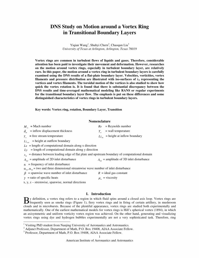
y definition, a vortex ring refers to a region in which fluid spins around a closed axis loop. Vortex rings are

frequently seen as smoke rings (Figure 1), fiery vortex rings and in firing of certain artillery, in mushroom

clouds and in microbursts. Because of the plentiful appearance, vortex rings are studied both experimentally and

mathematically. One of the earliest mathematical models for vortex rings is Hill’s spherical vortex (1894), in which

an axisymmetric and uniform vorticity vortex region was achieved. On the other hand, generating and visualizing

vortex rings using dye and hydrogen bubbles experimentally are not a very sophisticated task. Therefore, ring

1 Visiting PhD student from Nanjing University of Aeronautics and Astronautics.

2 Adjunct Professor, Department of Math, P.O. Box 19408, AIAA Associate Fellow.

3 Professor, Department of Math, P.O. Box 19408, AIAA Associate Fellow.

B


2

velocity, growth rate and vorticity distribution were extensively investigated (Maxworthy 1972). More models

(Lamb 1945; Saffman 1970) were developed thereafter based on these characteristics.

Figure 1: Smoke ring from a smoke chamber (Traitor 2006)

It is not until the arrival of high computational capacity and advanced experimental methods, such as 3-D PIV,

that make researchers able to study the instantaneous vortical structures in boundary layer flows. It is found that

many ring-like vortices exist in boundary layer and believed to play a significant role in turbulence generation and

sustenance. These vortex rings differ from the axisymmetric rings in many ways. For example, the axis loop is not

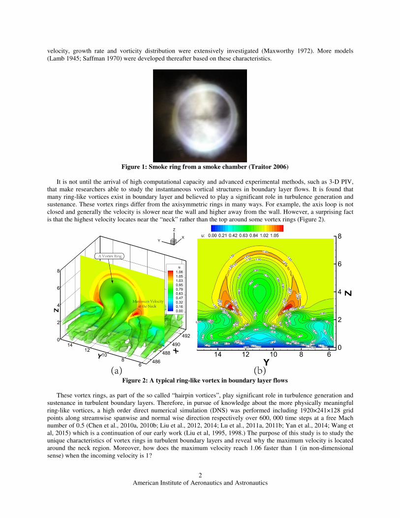
closed and generally the velocity is slower near the wall and higher away from the wall. However, a surprising fact

is that the highest velocity locates near the “neck” rather than the top around some vortex rings (Figure 2).

Figure 2: A typical ring-like vortex in boundary layer flows

These vortex rings, as part of the so called “hairpin vortices”, play significant role in turbulence generation and

sustenance in turbulent boundary layers. Therefore, in pursue of knowledge about the more physically meaningful

ring-like vortices, a high order direct numerical simulation (DNS) was performed including 1920×241×128 grid

points along streamwise spanwise and normal wise direction respectively over 600, 000 time steps at a free Mach

number of 0.5 (Chen et al., 2010a, 2010b; Liu et al., 2012, 2014; Lu et al., 2011a, 2011b; Yan et al., 2014; Wang et

al, 2015) which is a continuation of our early work (Liu et al, 1995, 1998.) The purpose of this study is to study the

unique characteristics of vortex rings in turbulent boundary layers and reveal why the maximum velocity is located

around the neck region. Moreover, how does the maximum velocity reach 1.06 faster than 1 (in non-dimensional

sense) when the incoming velocity is 1?


3

II. Case Setup and Code Validation

2.1 Case setup The computational domain is shown in Figure 3(a). The grid includes 1920×128×241 points in streamwise (x),

spanwise (y), and wall normal (z) directions respectively. A uniform grid is employed in both streamwise and

spanwise directions, while a stretching grid is used in normal direction. The first grid interval is carefully chosen to

make sure the grid is fine enough to capture all the small scales. The Message Passing Interface (MPI) plus the

streamwise direction domain decomposition which is shown in Figure 3(b) is utilized for parallel computation. The

flow conditions, including Reynolds number, Mach number, etc. are listed in Table 1. Lx and Ly are the lengths of

the computational domain in streamwise and spanwise directions, while Lzin is the height of the computational

domain at the inlet. xin is the distance between inlet and the leading edge of the flat plate and Tw represents the wall

temperature.

Table 1: Flow parameters

∞M 1000Re = 300 79in inx .= δ 798 03Lx .= δ 22in

Ly = δ 40in in

Lz = δ 273 15w

T . K= 273 15T .∞ =

0.5 1000 300.79 inδ 798.03 inδ 22 inδ 40 inδ 273.15K 273.15K

(a)

(b)

Figure 3. (a) Computational domain (b) Domain decomposition along the streamwise direction

2.2 Code Validation The code “DNSUTA” was developed at the University of Texas at Arlington and carefully validated by NASA

Langley and UTA researchers (Jiang et al., 2003; Liu et al., 2010b, Lu et al., 2011). The results have been compared

to experiments (Lee C B & Li R Q, 2007) and other’s DNS results (Rist et al., 2002), and the consistence shows our

results are correct and accurate. Since the detailed validation has been reported, only a brief describtion will be

given here.

2.2.1 Comparison with Log Law and grid convergence Time and spanwise-averaged streamwise velocity profiles for various streamwise locations in two different grid

levels are shown in Fig. 4. The inflow velocity profiles at x=300.79δin is a typical laminar flow velocity profile. At

x=632.33δin, the mean velocity profile approaches a turbulent flow velocity profile (Log law). This comparison

shows that the velocity profile from the DNS results is turbulent flow velocity profile and the grid convergence has

been realized.


4

(a) Coarse Grids (960x64x121) (b) Fine Grids (1920x128x241)

Figure 4. Log-linear plots of the time-and spanwise-averaged velocity profile in wall unit

2.2.2 Comparison with Experiment

By using λ2-eigenvalue visualization method, the vortex structures shaped by the nonlinear evolution of T-S

waves in the transition process are shown in Fig. 5. The evolution details are studied in our previous paper (Liu et al)

and the formation of ring-like vortices chains is consistent with the experimental work (Lee C B & Li R Q, 2007,

Fig. 6) .

Figure 5. Evolution of vortex structure at the late-stage of transition (Where T is the period of T-S wave)

z+

U+

100

101

102

103

0

10

20

30

40

50

x=300.79

x=632.33

Linear Law

Log Law


5

Figure 6. Evolution of the ring-like vortex chain

by experiment (Lee et al, 2007)

2.2.3 Comparison with Rist’s DNS data Fig. 7 shows a comparison of our DNS results with the data set provided by Rist as his personal kindness. The

comparison shows both DNS have same vortex structure. All these verifications and validations above show that our

code is correct and our DNS results are reliable.

(a) Our DNS (b) Rist’s DNS data

Figure 7. Comparison of our DNS results with Rist’s DNS data including vortex filaments and 2λ

All these verifications and validations above show that our code is correct and our DNS results are reliable.

III. DNS observation on vortex rings in boundary layer 1. The shape of vortex rings in boundary layer differs from axisymmetric vortex rings

The vortex rings in boundary layer has an open axis loop. Accordingly, the vortex filaments passing

through the vortex ring is not closed and originate from side boundaries as shown in Fig. 8. This unique

shape might be a decisive factor in the role vortex rings play in a boundary layer flow.


6

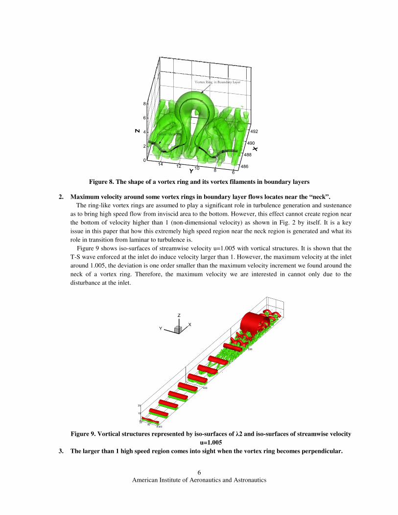
Figure 8. The shape of a vortex ring and its vortex filaments in boundary layers

2. Maximum velocity around some vortex rings in boundary layer flows locates near the “neck”.

The ring-like vortex rings are assumed to play a significant role in turbulence generation and sustenance

as to bring high speed flow from inviscid area to the bottom. However, this effect cannot create region near

the bottom of velocity higher than 1 (non-dimensional velocity) as shown in Fig. 2 by itself. It is a key

issue in this paper that how this extremely high speed region near the neck region is generated and what its

role in transition from laminar to turbulence is.

Figure 9 shows iso-surfaces of streamwise velocity u=1.005 with vortical structures. It is shown that the

T-S wave enforced at the inlet do induce velocity larger than 1. However, the maximum velocity at the inlet

around 1.005, the deviation is one order smaller than the maximum velocity increment we found around the

neck of a vortex ring. Therefore, the maximum velocity we are interested in cannot only due to the

disturbance at the inlet.

Figure 9. Vortical structures represented by iso-surfaces of λ2 and iso-surfaces of streamwise velocity

u=1.005

3. The larger than 1 high speed region comes into sight when the vortex ring becomes perpendicular.


7

The maximum streamwise velocity around ring-like vortices is not always around the neck region unless

the vortex rings become perpendicular enough. Fig. 10 shows three consecutive vortex rings and their

streamwise velocity distribution. The second ring-like vortex is identified as the same one shown in Fig. 2

and Fig.8 at earlier time steps. Fig. 10(c) shows the maximum streamwise velocity of this vortex ring is at

top of it which differs from its later configuration in Fig. 2. However, the first vortex ring in Fig. 10(a) is

more perpendicular with maximum velocity around the neck region shown in Fig. 10(b). For the third

vortex ring, which is oblique more obviously, the maximum velocity also locates at the top as illustrated in

Fig. 10(d).

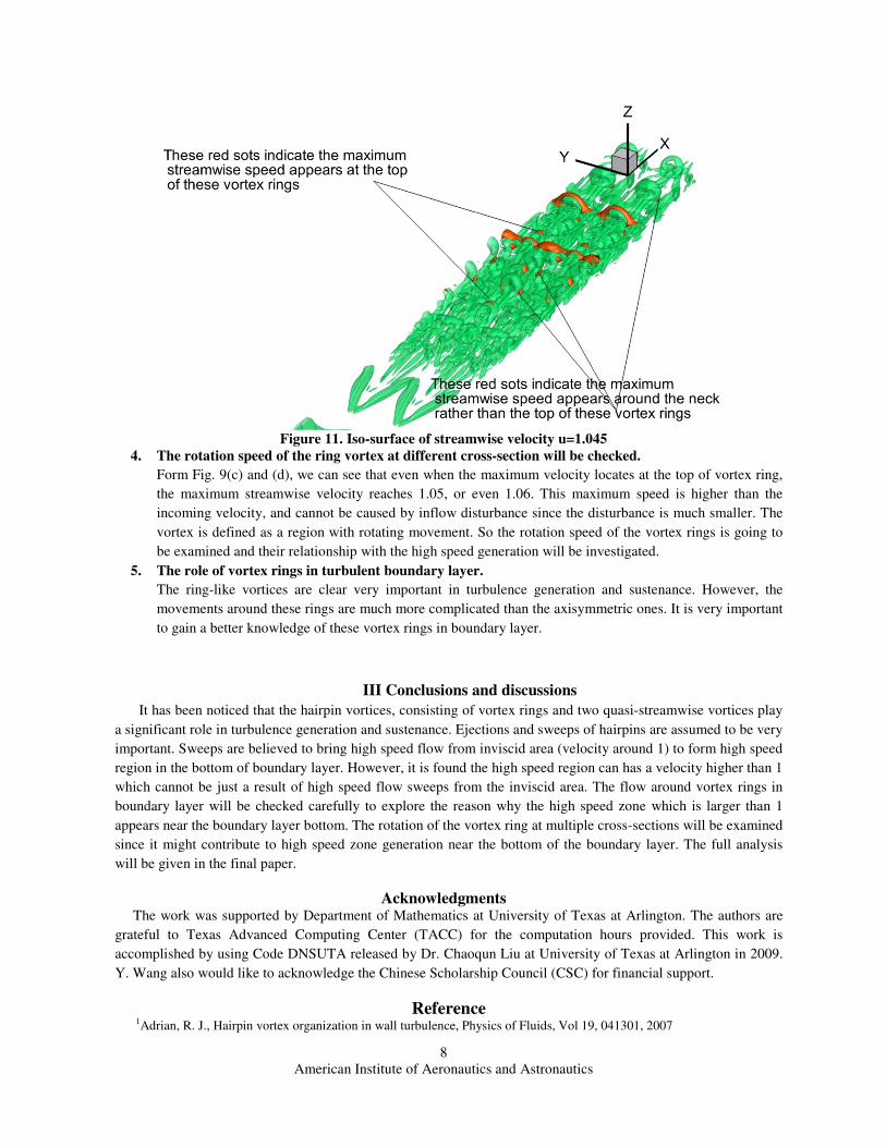
Fig. 11 shows the iso-surface of streamwise velocity u=1.045. It can be found that the maximum velocity

around some vortex rings locates around the neck region while the maxima around some rings are on the

top. Fig. 11 also verified the assumption that, when the ring is more perpendicular, the maxima tend to

locate at the neck region rather than on the top. Note that, for the rings in Fig. 11 with iso-surface of

streamwise velocity cover both the top and neck region, we cannot accurately determine where the

maximum velocity is just by this figure.

Figure 10. Three consecutive vortex rings and their streamwise velocity distribution


8

Figure 11. Iso-surface of streamwise velocity u=1.045

4. The rotation speed of the ring vortex at different cross-section will be checked.

Form Fig. 9(c) and (d), we can see that even when the maximum velocity locates at the top of vortex ring,

the maximum streamwise velocity reaches 1.05, or even 1.06. This maximum speed is higher than the

incoming velocity, and cannot be caused by inflow disturbance since the disturbance is much smaller. The

vortex is defined as a region with rotating movement. So the rotation speed of the vortex rings is going to

be examined and their relationship with the high speed generation will be investigated.

5. The role of vortex rings in turbulent boundary layer.

The ring-like vortices are clear very important in turbulence generation and sustenance. However, the

movements around these rings are much more complicated than the axisymmetric ones. It is very important

to gain a better knowledge of these vortex rings in boundary layer.

III Conclusions and discussions

It has been noticed that the hairpin vortices, consisting of vortex rings and two quasi-streamwise vortices play

a significant role in turbulence generation and sustenance. Ejections and sweeps of hairpins are assumed to be very

important. Sweeps are believed to bring high speed flow from inviscid area (velocity around 1) to form high speed

region in the bottom of boundary layer. However, it is found the high speed region can has a velocity higher than 1

which cannot be just a result of high speed flow sweeps from the inviscid area. The flow around vortex rings in

boundary layer will be checked carefully to explore the reason why the high speed zone which is larger than 1

appears near the boundary layer bottom. The rotation of the vortex ring at multiple cross-sections will be examined

since it might contribute to high speed zone generation near the bottom of the boundary layer. The full analysis

will be given in the final paper.

Acknowledgments The work was supported by Department of Mathematics at University of Texas at Arlington. The authors are

grateful to Texas Advanced Computing Center (TACC) for the computation hours provided. This work is

accomplished by using Code DNSUTA released by Dr. Chaoqun Liu at University of Texas at Arlington in 2009.

Y. Wang also would like to acknowledge the Chinese Scholarship Council (CSC) for financial support.

Reference 1Adrian, R. J., Hairpin vortex organization in wall turbulence, Physics of Fluids, Vol 19, 041301, 2007


9

2Chen, L., Liu, X., Oliveira, M., Liu, C., DNS for ring-like vortices formation and roles in positive spikes formation, AIAA

Paper 2010-1471, Orlando, FL, January 2010a. 3Chen L., Tang, D., Lu, P., Liu, C., Evolution of the vortex structures and turbulent spots at the late-stage of transitional

boundary layers, Science China, Physics, Mechanics and Astronomy, Vol. 53 No.1: 1−14, January 2010b, 4Dou, H.-S., Physics of flow instability and turbulent transition in shear flows, International Journal of Physical Science,

6(6), 2011, 1411-1425. 5Hama, F.R. and Nutant, J., 1963, Detailed flow-field observations in the transition process in a thick boundary layer. Proc.

1963 Heat Transfer & Fluid Mech. Inst. (Palo Alto, Calif.: Stanford Univ. Press) pp. 77-93. 6Hill, Micaiah John Muller. "On a Spherical Vortex." Proceedings of the Royal Society of London 55.331-335 (1894): 219-

224. 7Jiang, L., Chang, C. L. (NASA), Choudhari, M. (NASA), Liu, C., Cross-Validation of DNS and PSE Results for

Instability-Wave Propagation, AIAA Paper 2003-3555, The 16th AIAA Computational Fluid Dynamics Conference, Orlando,

Florida, June 23-26, 2003 8Lamb, Horace. "Hydrodynamics Dover." New York 43 (1945). 9Lee C B., Li R Q. A dominant structure in turbulent production of boundary layer transition. Journal of Turbulence, 2007,

Volume http://www.informaworld.com/smpp/title~db=all~content=t713665472~tab=issueslist~branches=8 - v88,

N 55 10Liu, C., and Liu, Z., Multigrid mapping and box relaxation for simulation of the whole process of flow transition in 3-D

boundary layers, J. of Computational Physics, Vol. 119, pp. 325-341, 1995. 11Liu, C., Chen, L., Lu, P., New theories on boundary layer transition and turbulence formation, J. of Modeling and

Simulation in Engineering, Volume 2012, ID 649419, 2012, Hindawi Publishing Corporation. 12Liu, C., Yan, Y. and Lu, P., Physics of turbulence generation and sustenance in a boundary layer, Computers & Fluids

102 (2014) 353–384. 13Liu Z., Xiong G, Liu, C., A contravarient velocity based implicit multilevel method for simulating the whole process of

incompressible flow transition around Joukowsky airfoils, J. of Applied Mechanics and Engineering, pp111-161, No. 1, Vol. 3,

1998. 14Lu, P. and Liu, C., Numerical study on mechanism of small vortex generation in boundary layer transition. AIAA Paper

2011-0287, 2011b 15Lu, P. and Liu, C., DNS Study on Mechanism of Small Length Scale Generation in Late Boundary Layer Transition,

Physica D: Nonlinear Phenomena, 241 (2012) 11-24, 2011c 16Maxworthy, T. "The structure and stability of vortex rings." J. Fluid Mech 51.1 (1972): 15-32. 17

Moin, P., Leonard, A. and Kim, J., Evolution of curved vortex filament into a vortex ring. Phys. Fluids, 29(4), 955-963,

1986 18Morton, T. S. "The velocity field within a vortex ring with a large elliptical cross-section." Journal of Fluid

Mechanics 503 (2004): 247-271. 19Rist, U., et al. Turbulence mechanism in Klebanoff transition: a quantitative comparison of experiment and direct

numerical simulation. J. Fluid Mech. 2002, 459, pp. 217-243. 20Robinson, S. K., 1991, “Coherent Motion in the Turbulent Boundary Layer,” Annu. Rev. Fluid Mech., 23, pp. 601–639. 21Saffman, Po G. "The velocity of viscous vortex rings(Small cross section viscous vortex ring velocity in ideal fluid with

arbitrary vorticity distribution in core)." Studies in Applied Mathematics 49 (1970): 371-380. 22Schoppa, W. and Hussain, F., Coherent structure generation in near-wall turbulence, J. Fluid Mech. 453 (2002), pp. 57–

108. 23Theodorsen, T., Mechanism of turbulence, Proceedings of the Midwestern Conference Fluid Mechanics, 1-19, Ohio State

University, Columbus, 1952. 24Traitor, smoke ring from smoke chamber, 2006. http://en.wikipedia.org/wiki/Smoke_ring 25Wallace, J.M., Highlights from 50 years of turbulent boundary layer research, Journal of Turbulence Vol. 13, No. 53,

2013, 1–70 26Wang, Y., Al-dujaly, H., Tang, J., & Liu, C. DNS Study on Hairpin Vortex Structure in Turbulence. AIAA Paper 2015-

1524, Orlando, FL, 2015. 27Wu, X. and Moin, P., Direct numerical simulation of turbulence in a nominally zero-pressure gradient flat-plate boundary

layer, JFM, Vol 630, pp5-41, 2009 28Yan, Y., Chen, C., Fu, H., Liu, C., DNS Study on λ-Vortex and Vortex Ring Formation in Flow Transition at Mach

Number 0.5. Journal of Turbulence, Vol 15(1), pp 1-21,2014

Documents

DNS Study on Motion around a Vortex Ring in Transitional ...Figure 8. The shape of a vortex ring and its vortex filaments in boundary layers 2. Maximum velocity around some vortex