Embed Size (px)
Citation preview
Do Bank-affiliated Analysts Benefit from Lending Relationships?
By Xiumin Martin
Abstract
This paper investigates whether private information from lending activities improves the
forecast accuracy of bank-affiliated analysts. Using a matched sample design, matching
by affiliated bank or borrower, we demonstrate that the forecast accuracy of bank-
affiliated analysts increases after the followed firm borrows from the affiliated bank. We
also find that the increase in forecast accuracy is more pronounced for borrowers with
greater information asymmetry and bad news, and for deals with financial covenants.
Last, we find that the informational advantage of bank-affiliated analysts exists only
when the affiliated banks serve as lead arrangers, not merely as participating lenders.
Overall our evidence suggests that information flows from commercial banking to equity
research divisions within financial conglomerates.
JEL: G14, G21, G24, G28
Key Words: Bank-affiliated analyst, conglomerate forecast, information sharing
*We would like to the editor, Abbie Smith, the anonymous referee, Douglas Skinner,
Terry Shevlin, Donal Byard, and workshop participants at Washington University in St.
Louis, Hong Kong University of Science and Technology, Singapore Nanyang
Technology University, and University of Texas at Dallas for their helpful comments.

2

1
1. Introduction
Since the 1990s, the financial industry in the United States has seen a wave of
mergers and acquisitions. Much of the consolidation has been spurred by the relaxation of
the Glass-Steagall provisions in the late 1980s and peaked after the passage of the
Gramm-Leach-Bliley Act (GLBA) in 1999. GLBA repealed the Glass-Steagall Act of
1933, which had separated commercial banking from investment banking and other types
of security dealing businesses. This financial industry consolidation resulted in
conglomerates that not only provide commercial lending service, but also engage in
securities dealing and market making businesses. As is well known, commercial banks,
thanks to their lending activities, have superior information about borrowers (e.g., Fama
[1985], James [1987], Petersen and Rajan [1994]).
In this paper, we investigate whether banks’ information advantage benefits their
affiliated security analysts by helping them make more accurate earnings forecasts.
Specifically, we ask two questions: First, do EPS forecasts by bank-affiliated analysts for
borrowers become more accurate after loan initiation? Second, if so, do we see cross-
sectional variation in the improvement of forecast accuracy that is related to borrower
characteristics and deal structure?
We investigate these questions using a sample of bank loans and analyst forecasts
for the period 1994 to 2007. For purposes of our analysis, we define conglomerate
analysts as security analysts who are affiliated with a commercial bank within a financial
conglomerate. A conglomerate analyst can issue earnings forecasts for firms that borrow
from the affiliated bank and firms that do not borrow from the affiliated bank. The former
are referred to as conglomerate forecasts. We employ a pre and post and matched-pair

2
research design in the paper. Specifically, we make a pre and post loan comparison in the
accuracy of conglomerate forecasts relative to benchmark forecasts issued by the same
analyst for firms that do not borrow from the affiliated bank. We also compare
conglomerate forecasts made during the pre and post loan period to benchmark forecasts
made by nonconglomerate analysts who follow the same borrower.
We document four main findings. First, the accuracy of conglomerate forecasts
increases after a firm borrows from the affiliated bank, and this increase is both
statistically and economically significant. Relative to benchmark forecasts, conglomerate
analysts reduce annual EPS forecast error by seven cents, which is about one sixth of the
average EPS forecast error in our sample. This result is robust to various model
specifications and controls. Second, the increase in the accuracy of conglomerate
forecasts after loan initiation is more pronounced for (1) borrowers with high information
asymmetry—that is, those characterized by small size and high standard deviation of
analyst EPS forecasts—and for (2) deals with financial covenants and high bank
ownership. Third, the informational advantage of conglomerate analysts is concentrated
among borrowers with bad news and high credit risk. Fourth, the informational advantage
for conglomerate analysts exists only when conglomerates serve as lead arrangers, not
merely as participating lenders. Taken together, our results suggest that there is
information spillover from the commercial lending divisions to the equity research
divisions of financial conglomerates and that bank-affiliated analysts benefit from this
information spillover via more accurate forecasts. Although information sharing is
beneficial to financial conglomerates, it is not without controversy, particularly when
much of the superior information comes from ongoing correspondence between

3
borrowers and banks.1 In recent years, regulators and market participants have expressed
concerns that the spillover of private information into the public domain might breach
confidentiality agreements between lenders and issuers and, more importantly, could lead
to illegal trading (Standard & Poor’s [2008]). Banks have tried to address this concern by
establishing limits to the flow of information among different parts of a financial
conglomerate, that is, erecting so-called Chinese Walls. Analysts, along with public
trading and sales desks that they are associated with, work on the public side of the wall
and are therefore not supposed to receive private information. Our findings suggest that,
despite the purported existence of Chinese Walls, financial analysts still have access to
superior information from lending relationships and exploit this access to improve their
forecast accuracy.
In this regard, our study is closely related to several recent papers that investigate
the information flow from the lending arm to other divisions of financial conglomerates
or sometimes even to outside parties. Acharya and Johnson [2007], for example, provide
evidence consistent with the use of private information by informed banks in the credit
default swap market. Similarly, Massa and Rehman [2008] show that a subset of bank-
affiliated mutual funds benefits from information sharing within a financial conglomerate.
Ivashina et al. [2009] find that the probability of a borrower being a target increases when
both the acquirer and the target have the same lender, suggesting information sharing
between the bank and potential acquirers. Our study adds to this stream of literature by
identifying a new channel of information sharing within financial conglomerates and
documenting the impact of this information sharing on analyst forecast accuracy.
1 The superior information may include material private information such as financial projections and plans
for mergers or acquisitions.

4
Our study also relates to several recent papers that document that institutional
investors as syndicate lenders trade on borrowers’ private information acquired from the
loan market (Bushman et al. [2010], Ivashina and Sun [2010], Massoud et al. [2010]).
Our findings suggest that borrowers’ private information can also be capitalized by
lender-affiliated security analysts to improve their forecast accuracy.
Our study also adds to the security analyst literature. A considerable amount of
literature examines the impact of investment banking ties or brokerage firm affiliation on
the properties of analyst forecasts and recommendations (e.g., Lin and McNichols [1998],
Michaely and Womack [1999], Bradley et al. [2003], and Cowen et al. [2006]). However,
little research focuses on how commercial banking ties affect the incentives and
performance of financial analysts. We fill this void by documenting that bank-affiliated
analysts increase forecast accuracy after the initiation of lending relationships between
followed firms and affiliated banks. The accompanying increase in forecast accuracy
could enhance the analysts’ job security and attract more investment advisory business
and trading volume to financial conglomerates.
Finally, our study has implications for policymakers. First, it speaks to the debate
regarding the reform of the banking industry in the 1990s, particularly on the repeal of
Glass-Steagall Act of 1933. So far, much of the evidence regarding the effects of the
repeal has focused on the consequences of housing lending and underwriting under the
same roof (e.g., Puri [1996], Gande et al. [1997, 1999], and Roten and Mullineaux
[2002]). Our study, together with Acharya and Johnson [2007], Ivashina et al. [2009], and
Massa and Rehman [2008], suggests that conflicts of interest may arise not only when
banks combine lending with underwriting but also when they engage in other types of

5
securities businesses such as equity research, trading, and investment advisory service.
Second, the U.S. Securities and Exchange Commission (SEC) implemented Regulation
FD (Fair Disclosure) on October 23, 2000, to prohibit firms from privately disclosing
value-relevant information to select securities markets professionals without
simultaneously disclosing the same information to the public. Although private
communications between lenders and borrowers are exempt from Regulation FD, sharing
of private information with analysts violates the spirit of the regulation and may warrant
regulators’ attention.
The rest of the paper is organized as follows. Section 2 develops testable
hypotheses. Sections 3 and 4 discuss sample selection and research methodology,
respectively. Section 5 presents empirical results and additional analyses. Section 6
discusses sensitivity tests, and section 7 concludes.
2. Literature review and hypotheses development
2.1. Background about the regulation changes in the banking industry
The Glass-Steagall Act of 1933 prohibited commercial banks from underwriting
and dealing in corporate securities. In the 1980s, the banking industry sought to repeal
Glass-Steagall. In 1987, the Federal Reserve permitted banks to establish Section 20
subsidiaries to engage in underwriting or dealing ―ineligible‖ securities. However,
Section 20 subsidiaries are subject to a substantial set of firewalls that limit information,
resource, and financial linkage between them and their parent holding companies as well
as their commercial banking affiliates. The Federal Reserve also limited to 5 percent of
the subsidiary’s total revenue the amount of revenue that a Section 20 subsidiary could
derive from bank ―ineligible‖ activities. The limit was raised to 10 percent in 1989 and

6
then to 25 percent in 1996. On November 26, 1999, Congress passed the GLBA, which
effectively repealed the Glass-Steagall Act. The GLBA expands the options available for
a financial conglomerate to engage in securities underwriting and dealing activities by
creating the financial holding company (FHC). Securities subsidiaries of FHCs do not
face the revenue constraints of Section 20s and are subject to far fewer firewall
constraints.
Over the course of 1990s and early 2000s, commercial banks acquired or merged
with investment banks and brokerage firms on a massive scale. In the United States alone,
about 10% of brokerage firms tracked by First Call (referred to as financial conglomerate
analysts in this article) were affiliated with commercial banks through the same parent
holding companies between 1994 and 2007.
2.2. Hypotheses development
Prior literature on financial intermediation highlights that banks have superior
information about borrowers that is not available to other market participants. Rajan
[1992], for example, shows that lending relationships generate valuable information
including "soft data" such as insights on the competence of management. Stein [2002]
echoes this point and argues that the unique characteristic of small-business lending is
that banks rely on the "soft data" generated by the lending relationship. Petersen and
Rajan [1994] likewise show that lending relationships reduce the asymmetric information
problem between the firm and its lender, with the positive effect of expanding the
availability of credit to firms. Chemmanur and Fulghieri [1994] argue that banks have an
incentive to spend resources obtaining private information and monitoring their

7
borrowing firms’ activities. Doing so enables them to evaluate whether to liquidate the
firm or renegotiate its loans when a firm undergoes financial distress.
Given that most of the information obtained from lending activities is nonpublic
and material, it is not surprising that regulators have long required banks to erect
―Chinese Walls‖ to limit the flow of this information within financial conglomerates.
However, evidence from prior studies suggests that Chinese Walls may not be totally
effective in preventing information spillover from the lending division to other divisions
of a financial conglomerate. Massa and Rehman [2008] find that lending relationships
affect portfolio allocation of bank-affiliated funds in a way that is consistent with bank-
affiliated funds exploiting superior information acquired from the lending side of their
parent company. Ivashina et al. [2009] also document information spillover: they find
that the probability of a borrower being a target increases when both the acquirer and the
target borrow from the same lender, suggesting information sharing between the lender
and the acquirer.
We hypothesize that information spillover may also exist from the lending division
to the equity research division within financial conglomerates. Inside information is
valuable to financial analysts as they have a strong incentive to forecast accurately. Keane
and Runkle [1998] note that ―… financial analysts’ livelihoods depend on the accuracy of
their forecasts…‖ Furthermore, Hong et al. [2000] show that inaccurate earnings
forecasts threaten security analysts’ careers. Consequently, when a brokerage firm is
affiliated with a financial conglomerate, its research analysts would have strong
motivation to obtain private information from the lending division about any borrower for
which they make forecasts.

8
Accurate forecasts can also benefit conglomerates by generating more trading
volume and attracting more investment advising business; Alford and Berger [1999], for
example, document a positive relation between brokerage commissions and analyst
forecast accuracy. Such benefits can to some extent disincentivize financial
conglomerates from strictly enforcing their Chinese Walls.2
Of course, any benefits reflected in more accurate equity research need to be
balanced against potential litigation and reputational costs associated with breaching the
Chinese Walls. However, we argue that during our sample period, the benefits from
information spillover were likely to exceed potential costs for at least three reasons. First,
insider trading can be difficult to prove in court. 3
Insider trading generally requires proof
of breaching a duty either based on a relationship or a confidentiality agreement.
Furthermore, evidence of insider trading is seldom straightforward. Instead, it tends to be
circumstantial and subject to inference and interpretation.4 Second, although borrowers
may bring cases against banks if they suspect that the banks misuse the confidential
lending information, they may have little incentive to do so when their capital providers
are on the giving end and research analysts (rather than their competitors or potential
suitors) are on the receiving end. Dass and Massa [2009] show that close banking
2 Note that information spillover from the lending division to the equity division does not necessarily
diminish the opportunities for financial conglomerates to capitalize their information advantage through
proprietary trading because they can time the release of analyst forecasts and proprietary trading.
3 For example, recently, a federal judge dismissed a high-profile insider-trading case against a Deutsche
Bank salesman and a hedge-fund trader, against whom the SEC brought enforcement action on the account
that they shared confidential information about a leveraged buyout deal and then traded credit swaps based
on that information. In dismissing the case, the US district judge John Koeltl wrote that, ―While the SEC
attempts to attribute nefarious content to those calls through circumstantial evidence, there is, in fact, no
evidence to support this inference and ample evidence that undercuts the SEC’s theory that the defendants
engaged in insider trading.‖ (Hurtado and Weidlich [2010]).
4 We thank Hillary Sale, a law professor at Washington University in St. Louis and corporate lawyer, for
discussion and insights relating to the legal issues involved in insider trading.

9
relationships increase borrowers’ firm value through banks’ active monitoring, which
further reduces borrowers’ motive to sue conglomerates. Third, due to the lack of staff at
the SEC, the regulator rarely brings enforcement actions against banks for misusing
lending information in equity research. These lines of argument lead to our first
hypothesis, formally stated as follows:
Hypothesis 1 (H1): The accuracy of conglomerate forecasts increases after loan
initiation.
When information asymmetry between firms and outsiders is large, banks are
likely to expend more resources and effort in screening and monitoring these firms due to
the lack of publicly available information. For this reason, a lending relationship is likely
to generate more private information for opaque firms compared with transparent firms.
Consistent with this view, Petersen and Rajan [1994], Berger and Udell [1995], and
Bharath et al. [2007] argue that durable relationships between lenders and borrowers can
attenuate information asymmetry for smaller firms. Slovin et al. [1992] find that, for
small firms, both loan initiation and renewal are associated with positive abnormal
returns when announced, while for large firms, neither initiation nor renewal has
significant excess returns. Based on this line of reasoning, we posit that lending
relationships have a greater impact on the accuracy of conglomerate forecasts when
borrower information asymmetry is high. The second hypothesis is stated formally as
follows:
Hypothesis 2 (H2): The accuracy of conglomerate forecasts increases more after loan
initiation for borrowers with high information asymmetry.
Since creditors' claims are more sensitive to bad news than good news (Smith
[1979]), banks are naturally more alert about potential deteriorations in borrowers'

10
financial positions. In addition, loan contracts often contain mechanisms (i.e., financial
covenants) through which bad news is revealed to lenders on a more timely basis than
good news. Consistent with these arguments, Acharya and Johnson [2007] show that the
information revealed by the credit default swap market is asymmetric and consists mainly
of bad news. Allen et al. [2009] find that the information about earnings is reflected in
loan prices four to five weeks prior to public earnings announcements and the pre-
announcement price movement is more pronounced for firms with bad news. Based on
these arguments, we posit that the information effect of lending relationships on the
accuracy of conglomerate analyst forecasts is more pronounced when firms experience
bad news. Our third hypothesis is formally stated as follows:
Hypothesis 3 (H3): The accuracy of conglomerate forecasts increases more after loan
initiation for borrowers with bad news.
When a loan contract imposes financial covenants, borrowers are required to
provide syndicate lenders timely covenant reports that often preempt information relevant
to loan pricing in upcoming quarterly earnings releases (Allen et al. [2009]). Furthermore,
lenders are more likely to include financial covenants in loan contracts for more
informationally opaque borrowers (Standard & Poor’s [2008], Bradley and Roberts
[2004], Chava et al. [2009], Bushman et al. [2010]). Both arguments suggest that
syndicate lenders have a greater information advantage when a loan contract includes
financial covenants. Therefore, our fourth hypothesis is stated as follows:
Hypothesis 4 (H4): The accuracy of conglomerate forecasts increases more after loan
initiation when a loan includes financial covenants.
The majority of the loans issued during our sample period and covered by
Dealscan are syndicated loans. An important feature of a loan syndicate is that the lead

11
arranger and the other participating banks play different roles and receive different
information. Lead arrangers establish and maintain a relationship with the borrower by
taking on the primary role of information collection and monitoring. In contrast, the other
participants rarely directly negotiate with the borrower, maintaining an arm’s-length
relationship and communicating through the lead arranger (Sufi [2007]). Bushman and
Wittenberg-Moerman [2009] note that soft information collected by the lead arranger in
the process of screening and monitoring the borrower is not available to uninformed
investors. Because soft information is costly to process, the lead arranger may have an
incentive not to disclose it to other syndicate participants in order to retain an information
advantage. Since the possession of information advantage by banks is the key argument
underlying our previous hypotheses, we restrict attention to single-lender loans or
syndicated loans where financial conglomerates act as lead arrangers when testing
hypothesis 1-4.
One could argue that every member of a syndicate has the same right to the
information gathered by the lead arrangers and that this information is actively shared
electronically (Acharya and Johnson [2007]). Therefore, participating lenders can have
private information about a borrower that resembles what the lead arranger has. If this is
true, the forecast accuracy of financial conglomerates that act as participating lenders
may also increase after a loan initiation. Given the two-sided argument regarding the
information advantage of the participating lenders, we state the next hypothesis in the
null form.
Hypothesis 5 (H5): The forecast accuracy of a financial conglomerate does not increase
after loan initiation when a conglomerate acts as a participating bank in a
syndicated loan.
12
3. Data and sample construction
3.1 Sample banks and their securities subsidiaries
We are interested in instances where a firm borrows from a financial
conglomerate and is covered concurrently by an analyst affiliated with that financial
conglomerate. We start our sample selection with a list of financial conglomerates and
their securities subsidiaries obtained from the Federal Reserve Board.5 There are 85
securities subsidiaries, associated with 62 financial conglomerates, as of December 2008.
We then manually match these securities subsidiaries with broker names in First Call’s
Broker ID file. We identify 32 matches. These 32 securities subsidiaries, along with the
27 financial conglomerates that they are affiliated with, constitute our initial list of
sample banks. Panel A of Appendix A provides a list of these financial conglomerates
and their securities subsidiaries.
Many of the sample banks and their securities subsidiaries are products of
mergers and acquisitions throughout the 1990s and beyond. This adds at least two
complications to our data construction: first, when measuring lending relationships
between a bank and its borrowers, we need to account for lending relationships inherited
via acquisitions. Second, some securities subsidiaries were acquired by their parent banks
during our sample period. In these cases, we need to ensure that the potential information
sharing between a securities subsidiary and its parent bank’s lending unit did not start
until the acquisition was completed. To tackle these complications, we use the SDC
Mergers and Acquisitions database to identify all merger/acquisition transactions
5 http://www.federalreserve.gov/generalinfo/subsidiaries/

13
involving our sample banks or their predecessors that were completed between 1991 and
2008.6 Based on the SDC data, we then construct a merger history tree for each of our
sample banks, focusing on those transactions that would have implications for our data
construction. Figure 1 provides an illustration of the merger history tree using Bank of
America as an example. We refer back to this example when we later explain how the
aforementioned two complications are dealt with based on the merger history compiled in
this step.
3.2 Bank loans
Bank loans are obtained from the Loan Pricing Corporation’s (LPC) Dealscan
database. The database provides detailed information on syndicated loans and single-
lender loans, including lenders’ identities, loan sizes and maturities, facility start and end
dates etc. We focus on loans initiated by the sample banks between Jan. 1, 1994, and Dec.
31, 2007, to nonfinancial firms (excluding firms identified with 2-digit SIC codes 60
through 70). The cut-off date of Dec. 31, 2007, is chosen because we require at least one
earnings forecast to be issued after a loan inception and EPS forecasts data from the First
Call end in 2008. We choose Jan. 1, 1994, as the beginning date of loan initiation for two
reasons: first, most of financial conglomerates were formed in the 1990s; second, the
coverage of First Call was not stable until 1993.
To account for the lending relationship inherited from acquired banks, we assume
that acquiring banks assume the lending relationships of their targets when a
6 The reason we start searching M&A deal announcements in the financial industry from 1991 is to ensure
the accuracy of identifying conglomerate analysts. Our sample analyst forecasts start from 1993 and it
usually takes about one or two years to complete an acquisition.

14
merger/acquisition is completed.7 Besides the above requirements, a deal-lender facility
is included in our sample if it also satisfies the following criteria: (1) borrowers are public
non-financial U.S. companies and their financial information is available in the
Compustat annual database;8 (2) it is the first lending relationship between the lender and
the borrower since 1990 or the maturity date of the previous loan and the starting date of
the current loan for the same lender-borrower pair are at least one year apart;9 (3) the
lending bank is either the sole lender or the lead arranger in a syndicated loan; 10,
11
(4)
the lending bank owns at least 10% of a loan.12
3.3 Analysts forecasts data
7 For example, Bank of America acquired FleetBoston on October 27, 2003 as illustrated in Figure 1. If
there are any outstanding loan deals between FleetBoston and its borrowers as of October 27, 2003, we
assume that this relationship is inherited by Bank of America and set October 27, 2003 as the loan initiation
date for all the outstanding loans. This assumption is based on the belief that the affiliated analysts of
acquiring banks will not have access to the private information of acquired banks’ borrowers until the
completion of acquisitions. 8 We thank Michael Roberts for providing Dealscan-Compustat link data. For details on the construction
and usage of the data, please see Chava and Roberts [2008]. 9 We impose this requirement because these deals are more likely to generate substantial amount of new
information for lending banks and there is less ambiguity in attributing the information effect to the current
loan rather than the previous one. 10
We classify a lender as a lead arranger if the lender’s role is not participant, technical, packager or
secondary investor. 11
In testing hypothesis 5, we require that financial conglomerates are participant lenders instead of lead
arrangers. All other sample selection procedure remains the same. Specifically, we require a sample deal
with a financial conglomerate as a participating lender and this deal is either the first deal or a deal whose
start date is at least one year apart from the maturity date of the prior deal for the same lender-borrower pair.
Note that the affiliating bank can be a lead arranger or a participating lender in the prior deal. Further, all
sample deals are still required to have at least one lead arranger with 10% ownership because participant
lenders rely on information provided by lead arrangers (Jones et al., 2005) and higher loan ownership
increases lead arrangers’ incentive to acquire private information to monitor borrowers. Then we obtain
earnings forecasts for both affiliated analysts and matched benchmarks (matched by affiliating banks or
borrowing firms) and form the broker constant sample and the firm constant sample, respectively. 12
Criteria (3) and (4) are imposed to make sure that lending banks have incentives to gather necessary
information on the borrowing firms, which is the primary condition for testing the first four hypotheses.
Similar criteria are imposed in prior studies (e.g., Massa and Rehman [2008], Mora and Sowerbutts
[ 2008]).

15
We obtain analysts annual EPS forecast data from the First Call Historical
Database.13
The actual earnings are also collected from First Call to be consistent with
forecasts in the treatment of nonrecurring items. For each deal-lender facility identified in
the previous step, we gather conglomerate analyst forecasts (if any) for the borrowing
firm made during the one-year period prior to and after a loan initiation date.14
We delete
those loan deals where conglomerate analysts provide no forecasts for the borrowing
firms during the one-year period either before or after the loan initiation day.
Table 1 summarizes our sample selection process in detail. After imposing the
above selection criteria, our final loan sample contains 418 unique deal-lender facilities
and 382 unique loan facilities. During our sample period (1994 through 2007), there are
24,988 unique loan facilities in the LPC database where borrowers are Compustat
nonfinancial firms and 7,109 unique loan facilities with loan ownership data available.
The total loan value of these 7,109 deals amounts to US$1.65 trillion. Of these, 4,396
(US$1.41 trillion) deals have at least one lead arranger with an equity research division
and 1,257 (US$0.64 trillion) deals have at least one lead arranger whose analysts issue
conglomerate forecasts. Thus our final sample of 382 unique loan facilities, which
amounts to $US0.26 trillion, is equivalent to 40% of the value of the loans with
conglomerate forecasts and ownership data available that are more relevant for our
study. While economically significant, our results need to be interpreted with caution
13
If an analyst issues multiple annual EPS forecasts with different forecasting period ends on the same day,
we keep the one with the closest forecasting period end. 14
Following Massa and Rehman [2008] who examine holdings of bank-affiliated mutual funds over a six-
month period prior to and after a loan initiation, we choose one-year period to investigate analyst earnings
forecasts. Furthermore, forecasts issued in the year before loan initiation will not be affected by the
information obtained from previous lending relationship due to the requirement of one-year separation
between two adjacent loans.

16
with regard to the representativeness of our findings for all banks issuing conglomerate
forecasts.
[Insert Table 1]
4. Methodology
4.1 Matched sample design
We’re interested in whether private information generated by lending activities
helps financial-conglomerate analysts improve their forecast accuracy. Part of our
research design involves comparing the accuracy of conglomerate forecasts in the post
loan-initiation period to that in the pre loan-initiation period. However, such pre/post
comparison may be confounded by changes in lender or borrower characteristics or both
or a general trend in forecast accuracy. To mitigate these confounding factors, we employ
a matched sample design and construct two sets of benchmark forecasts to compare with
the conglomerate forecasts.
The first set of benchmark forecasts, defined as the broker-constant sample,
consists of forecasts made by the same conglomerate analysts for matching nonborrowing
firms. A set of matching nonborrowing firms is identified for the borrowing firm in a
deal-lender facility in the following way. First, we identify all nonborrowing firms
followed by the analysts in the same financial conglomerate during the loan initiation
year that are within the same industry (measured by 2-digit SIC code) as the borrowing
firm. Nonborrowing firms are defined as firms in Compustat universe that do not borrow
from any of the 27 financial conglomerate banks listed in Panel A of Appendix A. We
further require that the selected nonborrowing firms be followed by the bank-affiliated

17
analysts during both the pre and post loan-initiation periods and have financial data
available from Compustat. Among the firms that satisfy these criteria, we choose five
with the closest total assets to the borrowing firm at the fiscal year-end prior to loan
initiation as the matching firms.15
This matching yields 1,868 unique matched pairs for
the 418 deal-lender facilities previously identified. The loan initiation year of the
borrowing firm is hypothetically assigned to the matching nonborrowing firm. As shown
in Table 1, conglomerate analysts issued a total of 19,363 unique forecasts for the
matching nonborrowing firms and 4,509 unique forecasts for the borrowing firms during
the one-year period prior to and after loan initiation. These 23,872 unique forecasts
constitute our broker-constant sample. This sample has the advantage of controlling for
the impact of brokerage characteristics and any general trend in analyst forecast accuracy.
The second set of benchmark forecasts, defined as the firm-constant sample,
consists of forecasts made by matching nonconglomerate analysts for the same borrowing
firms. Specifically, for each deal-lender facility, we first identify all nonconglomerate
analysts that follow the same borrowing firm during both the pre and post loan-initiation
periods. Among these analysts, we choose the five analysts with the closest number of
firms being followed (in the deal initiation year) compared with the conglomerate analyst.
16,17 We find matching nonconglomerate analysts for 376 out of the 418 deal-lender
facilities previously identified. These nonconglomerate analysts issued a total of 4,041
15
Lee [1997], Lyon et al. [1999] and Chan et al. [2004] suggest that using one control firm leads to noisy
point estimates. Since our paper focuses on testing corporate finance theory, the noise from low power
methods is of primary concern. Therefore, we follow their suggestion and use multiple control firms to
reduce the noise in single benchmark and increase the power of our tests.. 16
Our results are qualitatively similar when each deal-lender facility is matched with one or three non-
borrowing firm(s) for the broker-constant sample and one or three non-conglomerate analyst(s) for the
firm-constant sample. 17
For borrowers with fewer than five analysts following, we use all these analysts as benchmarks for the
conglomerate analyst in the firm-constant sample.

18
unique forecasts for the borrowing firms during the two-year period surrounding the loan
initiation, while conglomerate analysts issued a total of 16,627 unique forecasts. These
20,668 forecasts comprise our firm-constant sample. The advantage of this matching
procedure is that it controls for correlated omitted borrower characteristics and any
general trend that may affect analyst forecast accuracy.
4.2 Regression models for lending relationship and conglomerate analyst forecast
accuracy
Our first set of tests investigates whether the accuracy of conglomerate forecasts
improves relative to that of benchmark forecasts after loan initiation. We estimate the
following OLS model for the broker-constant sample and the firm-constant sample,
respectively. To control for invariant firm/broker characteristics and year specific shocks
that may affect analyst forecast accuracy, we include firm and year fixed effects for the
broker-constant sample and broker and year fixed effects for the firm-constant sample in
all estimations. In addition, heteroscedasticity-consistent standard errors clustered at the
firm level are used to derive p values.
ERROR = β0 + β1POST + β2CONGLOMERATE* POST + γCONTROLS +ε (1)
where ERROR is measured as the absolute difference between an analyst forecast and
actual earnings deflated by the stock price at the beginning of the forecast month
(Mikhail et al. [1999]). POST is a dummy variable that equals 1 if a forecast is issued
during the post loan-initiation period and 0 otherwise. Recall that nonborrowing firms
assume the loan initiation date from their matched borrowing firms in the broker-constant
sample. CONGLOMERATE is a dummy variable that equals 1 for conglomerate forecasts

19
and 0 for benchmark forecasts. Due to the way that we constructed our benchmark
samples, there is no variation in CONGLOMERATE within a firm for the broker constant
sample and no variation in CONGLOMERATE within an analyst for the firm-constant
sample. Consequently, firm fixed effects and broker fixed effects subsume the estimation
of CONGLOMERATE for both samples18 , 19
Although the coefficient on CONGLO-
MERATE cannot be estimated in our fixed effects regressions due to its time invariant
nature, the estimation of our main variable of interest, POST*CONGLOMERATE is not
affected by the inclusion of firm/broker fixed effects since CONGLOMERATE is
interacted with POST that changes over time. Based on Hypothesis 1, we expect the
coefficient on POST*CONGLOMERATE to be negative (i.e. β2<0).
CONTROLS includes a set of firm characteristics and forecast characteristics
identified in the prior research that are associated with forecast accuracy. First, firm
characteristics include log market value (LOGMKT), market-to-book ratio (MB), the
probability of loss (PLOSS), and a dummy for earnings increase (EPSUP). We expect
larger firms, firms with lower market to book ratio, lower probability of losses, and
earnings increases to have more accurate earnings forecasts. Second, we include the
number of analysts following a firm (LOGNUMANALYST) in year t as another control
variable. On the one hand, prior research finds that consensus forecast accuracy is
positively associated with the number of analysts following a firm (Alford and Berger
[1999]). To the extent that consensus forecast accuracy reflects the individual analyst
18
The inability to estimate the coefficients on the time-invariant variables has long been recognized as a
disadvantage of the fixed effects model. As Greene [2008] points out, "this lack of identification is the
price of the robustness of the specification to unmeasured correlation between the common effects and the
exogenous variables". 19
All our results (except for the forecast optimism test based on the broker-constant sample) are robust to
the exclusion of firm or broker fixed effects, where the coefficient on CONGLOMERATE can be separately
estimated.

20
ability, it implies a negative relation between the number of analysts following and
forecast error. On the other hand, Bhushan [1989] argues that investor demand for analyst
coverage is greater for firms with greater share price volatility, because the potential
investor gains from firm-specific information are greater for these firms. If analyst
coverage is positively related to stock price volatility as Bhushan argues, we may instead
observe a positive association between the number of analysts following and forecast
error since greater price volatility can lead to larger forecast errors. Third, many prior
papers identify the age of forecasts as being negatively associated with forecast accuracy
(e.g., Brown et al. [1987], O’Brien [1988], Clement [1999]). We use HORIZON,
measured as the number of days between the forecast date and the earnings
announcement date, to control for this effect. We also control for the number of months
for which an analyst has been following a firm before the current year (LOGEXP) and
expect it to be negatively associated with forecast error (Mikhail et al. [1997], Clement
[1999]). The effect of analyst learning on forecast accuracy could diminish with
experience. Therefore we include a square term of experience and expect a positive
coefficient on this term. All firm level control variables are measured at the end of the
fiscal year prior to the issuance of an EPS forecast. A more detailed description of these
variables and their measurement is provided in Appendix B. All continuous variables are
winsorized at 1% and 99% levels.
Hypothesis 2 predicts that increases in the accuracy of conglomerate forecasts are
more pronounced for borrowers with high information asymmetry. To test this hypothesis,
we employ two measures of information asymmetry used in the previous literature. The
first measure is total market value of equity measured at the fiscal year prior to loan

21
initiation (LOGMKT); the second measure is the standard deviation of analyst annual
earnings forecasts made in the fiscal year prior to loan initiation (STD DEV). Using these
two measures, we estimate model (1) for the two subsamples partitioned based on the
sample median of LOGMKT or STD DEV, respectively.
If Hypothesis 2 holds, we would expect the coefficient on CONGLOMERATE*
POST to be more pronounced for the subsample of small firms (i.e. firms with LOGMKT
below the corresponding sample median) and the subsample of firms with a high standard
deviation of analyst earnings forecasts (i.e. firms with STD DEV above the corresponding
sample median).
Furthermore, Hypotheses 3 and 4 predict that increases in the accuracy of
conglomerate forecasts are more pronounced for borrowers with bad news and for loans
with financial covenants. To test the bad news hypothesis, we partition the broker-
constant sample (the firm-constant sample) into two subgroups based on positive or
negative stock return of a borrower in the year that an EPS forecast is issued, where the
annual stock return is cumulative abnormal stock return over a fiscal year. To test the
covenant hypothesis, we adopt a similar approach and partition the broker-constant
sample (the firm-constant sample) into two subgroups based on whether a loan contains a
financial covenant. We then rerun model (1) for both subgroups under each partition. If
these two hypotheses hold, the coefficient on CONGLOMERATE *POST should be
greater for the subgroup of firms with bad news and for the subgroup of loans with
financial covenants.
Hypothesis 5 tests whether forecast accuracy increases after loan initiation for
financial conglomerates that act as participant lenders. To test this hypothesis, we
22
construct a parallel broker-constant sample and firm-constant sample for participant
lenders as described in Footnote 9 and re-estimate model (1) for the new samples.
5. Empirical results
5.1 Summary statistics
Table 2 reports the summary statistics for the main variables for the broker-
constant sample and the firm-constant sample. The summary statistics for all variables
are similar across the two samples, so we only focus on the broker-constant sample.
Analyst forecast errors (ERROR) are right skewed with a mean of 0.014 and a median of
0.004, comparable with that reported in Mikhail et al. [1999]. As a result of our research
design, the number of benchmark forecasts (81.1% of the broker-constant sample) is
slightly less than five times that of conglomerate forecasts (18.9% of the sample). On
average, bank-affiliated analysts issued similar numbers of forecasts in the one-year
period before and after the loan initiation. Two size variables are also highly skewed: the
mean (median) market value (MKT) is 9,316 (2,907) millions and the mean (median)
asset size (ASSETS) is 8,949 (2,623) millions.20
The mean (median) market-to-book (MB)
ratio is 3.29 (2.51). The average predicted probability of loss (PLOSS) for the broker-
constant sample is about 13.3%, while 57.1% of observations report an earnings increase
(EPSUP) during the fiscal year prior to analyst forecasts. There are, on average, 11
analysts following the sample firms over the course of a fiscal year (NUMANALYST) and
the average forecast horizon (HORIZON) and forecast experience (EXPERIENCE) are
298 days and 59.3 months respectively. Finally, about 37.3% of forecasts are issued for
20
Compared to Sufi [2007] and Ball et al. [2008], our sample firms are much larger. This is expected given
all our sample banks are large financial conglomerates and therefore are more likely to have large
borrowers.

23
investment grade firms (INVEST) and about 55.5% of firm-years experience negative
abnormal return (BADNEWS) during the forecast year.
Regarding deal characteristics, the mean (median) bank ownership of a loan is
24.9% (16%). About 62.4% of deals have at least one financial covenant. Conditional on
the existence of a financial covenant, the average number of financial covenants in the
sample is 1.21.
[Insert Table 2]
Table 3 presents the correlation matrix for the variables used in our analyses for
the broker-constant sample (Panel A) and the firm-constant sample (Panel B). Pearson
(Spearman) correlations are displayed in the lower (upper) diagonal. CONGLOMERATE
is negatively correlated with ERROR in the broker constant sample and positively
correlated with ERROR in the firm constant sample. In general larger firms and firms
with more growth opportunities, more analyst following, lower leverage, better
performance, and smaller standard deviation of analyst EPS forecasts have more accurate
analyst forecasts. All of these results are consistent with our predictions. In addition
analysts with more forecasting experience for a firm provide more accurate forecasts.
Analyst forecasts are also more accurate for investment grade firms than for non-
investment grade firms.21
[Insert Table 3]
5.2 Univariate results
21
Note that the high correlation between LOGMKT and LOGNUMANALYST is of concern and may cause
biased coefficient estimates. To address this concern, we further check VIFs for these variables based on
model (1) and the VIF for LOGMKT is 3.11, which are much lower than 10. Therefore multicollinearity is
not likely to be a problem in interpreting the results.

24
In Table 4, we compare properties of conglomerate forecasts with those of
benchmark forecasts in the pre and post loan-initiation periods. For the broker-constant
sample (Panel A of Table 4), the mean conglomerate forecast error is 0.0133 in the pre
loan-initiation period, which is not statistically different from the mean benchmark
forecast error (0.0136) during the same period. In contrast, after loan initiation, the
conglomerate forecast error decreases by 0.0011 to 0.0123, while the benchmark forecast
error increases by 0.0015 to 0.0151. Both changes are statistically significant. Looking at
the medians, conglomerate forecast error decreases from 0.0039 to 0.0038 after loan
initiation. However, the change is not statistically significant based on Wilcoxon sign-
rank test. The median benchmark forecast error increases from 0.0041 to 0.0043 after
loan initiation, and the increase is statistically significant at 5% level.
Turning to the firm-constant sample (Panel B of Table 4), the mean conglomerate
forecast error decreases significantly from 0.0123 before loan initiation to 0.0102 after
loan initiation at the .01 level, while the benchmark forecast error increases significantly
from 0.0130 before loan initiation to 0.0160 after loan initiation. When focusing on
medians, the error of conglomerate forecasts decreases from 0.0040 before loan initiation
to 0.0039 after loan initiation, and the decrease is statistically significant at 10% level
based on Wilcoxon sign-rank test. By comparison, the median benchmark forecast errors
remain unchanged after loan initiation. Taken together, the univariate evidence from both
the broker-constant sample and the firm-constant sample is consistent with the prediction
of Hypothesis 1 that the accuracy of conglomerate forecasts improves relative to
benchmark forecasts after loan initiation.

25
Table 4 also provides information on the control variables for conglomerate
forecasts and benchmark forecasts. Underscoring the importance of controlling for these
variables in the multivariate analysis, most control variables are significantly different
across conglomerate forecasts and benchmark forecasts or across the pre and post loan-
initiation periods.
[Insert Table 4]
5.3 Multivariate regression results
5.3.1 The association between conglomerate analyst forecast accuracy and loan
initiation
Table 5 presents regression results for model (1). The estimated results for the
broker-constant sample are reported in columns 1 and 2 of Table 5. The coefficient on
POST is insignificant suggesting little change in benchmark forecasts accuracy after loan
initiation. In contrast, the coefficient on CONGLOMERATE*POST is negative and
statistically significant at less than 5% level (β3= -0.002, p=0.012). This is consistent with
Hypothesis 1 that the accuracy for conglomerate forecasts increases after loan initiation
relative to that of benchmark forecasts made by the same analysts for nonborrowing firms.
Helping to put the above estimates in economic perspective, the mean stock price
of the broker-constant sample is $34. Thus a 0.002 reduction in forecast error relative to
the benchmark forecasts translates to about 7 cents of improvement in forecast accuracy,
which is not only statistically but also economically significant. Another way to evaluate
the materiality of the above estimate is to compare it with the mean forecast error for the
overall sample. The mean ERROR in the pre loan period is 0.013 for the broker-constant
sample as shown in Table 4. Thus a 0.002 reduction in forecast error represents nearly a
one-sixth improvement in forecast accuracy relative to an average forecast.

26
The estimated coefficients for the control variables are largely consistent with our
predictions: larger firms as well as firms with lower market-to-book ratios, lower
probabilities of losses, and earnings increases are associated with more accurate forecasts.
In addition, greater analyst following leads to larger forecast errors, which is consistent
with the argument in Bhushan [1989]. Analyst forecasts are more accurate when they are
issued closer to earnings announcement dates. The coefficient on analyst experience is
inconsistent with our predictions for the broker-constant sample but consistent for the
firm-constant sample.22
Finally, the coefficient on the square term of analyst experience
is positive and consistent with our predictions for both the broker-constant sample and
the firm-constant sample.
[Insert Table 5]
The estimated results for the firm-constant sample—reported in columns 3 and 4
of Table 5—are both quantitatively and qualitatively similar to those based on the broker-
constant sample. The accuracy of benchmark forecasts does not change after loan
initiation as indicated by the insignificant coefficient before POST. More importantly, the
coefficient on CONGLOMERATE*POST is negative and statistically significant at less
than 5% level, (β2= -0.002, p=0.017), suggesting that the accuracy of conglomerate
forecasts improves relative to benchmark forecasts after loan initiation.
Overall, the results in Table 5 corroborate the univariate evidence presented in
Table 4 and provide support for Hypothesis 1: regardless of the benchmark forecasts used,
the accuracy of conglomerate forecasts significantly improves after loan initiation relative
to benchmark forecasts.
22
However, the estimate of this coefficient is sensitive to the inclusion of firm fixed effects. When we re-
estimate model (1) for the broker-constant sample without controlling for firm fixed effects, the coefficient
on analyst experience has the predicted sign.

27
5.3.2 The association of conglomerate analyst forecast accuracy with loan initiation and
borrower information asymmetry
Table 6 reports the estimated results for tests of hypothesis 2 for the broker-
constant sample and the firm-constant sample using firm size (Panel A) and the standard
deviation of analyst forecasts (Panel B) as proxies for information asymmetry,
respectively. Since the estimated results are qualitatively similar across the two samples,
we focus our discussion on the results estimated from the broker-constant sample. The
coefficient on CONGLOMERATE *POST is significantly negative for the subsample of
small firms (β2= -0.002, p=0.030) and the subsample of firms with the standard deviation
of analyst forecasts above the sample median (β2= -0.005, p<0.001), while it is
indistinguishable from 0 for the subsample of large firms and the subsample of firms with
the standard deviation of analyst forecasts below the sample median. Therefore, the
evidence supports Hypothesis 2 that the improvement in the accuracy of conglomerate
forecasts after loan initiation relative to benchmark forecasts is more pronounced for
borrowers with poorer information environment.
[Insert Table 6]
5.3.3 The association of conglomerate analyst forecast accuracy with loan initiation and
the type of news
Hypothesis 3 predicts that the information effect of a lending relationship on
conglomerate forecast accuracy is stronger for borrowers experiencing bad news. The
estimated results are summarized in Table 7. Consistent with our prediction, the
coefficient on CONGLOMERATE*POST is negative and statistically significant for firms
with bad news (columns 3, 4, 7, and 8). In contrast, the same coefficient is not
distinguishable from 0 for firms with good news (columns 1, 2, 5, and 6).

28
[Insert Table 7]
5.3.4 The association of conglomerate analyst forecast accuracy with loan initiation and
existence of financial covenants
Hypothesis 4 conjectures that the accuracy of financial conglomerate forecasts
increases more when a loan deal contains financial covenants. Table 8 reports the test
results for this hypothesis. For deals with financial covenants, the coefficient on our main
variable of interest, CONGLOMERATE*POST is significantly negative, (β2= -0.003,
p=0.005 for the broker constant sample (columns 1 and 2); β2= -0.002, p=0.060 for the
firm constant sample (columns 5 and 6). Conversely, for deals without financial
covenants, the coefficient on CONGLOMERATE*POST is not distinguishable from 0
(columns 3, 4, 7, and 8). This provides support for Hypothesis 4 that the accuracy of
financial conglomerate forecasts increases more when a deal contains financial covenants.
These results are also consistent with the findings in prior studies that the existence of
financial covenants enables lenders to have more timely access to firms’ nonpublic
information (Bushman et al. [2010], Massoud et al. [2010]).
[Insert Table 8]
5.3.5 The association of conglomerate analyst forecast accuracy with loan initiation
when banks are participant lenders
Table 9 reports the test results of Hypothesis 5 based on the two samples for
participant lenders as described in Footnote 9. As can be seen, the coefficient on
CONGLOMERATE*POST is positive but statistically indistinguishable from 0 for both
samples, suggesting no information spillover effect after loan initiation. Therefore,
consistent with the arguments of Sufi [2007] and Bushman and Wittenberg-Moerman

29
[2009], we do not find that participant lenders have a similar information advantage as
lead arrangers.
[Insert Table 9]
5.4 Additional analyses
5.4.1. The association of conglomerate analyst forecast optimism with loan initiation
Though our focus is on analyst forecast accuracy, we also investigate how lending
relationships affect analyst optimism. Prior studies show that analysts could issue
optimistic forecasts to please firms’ managers in order to obtain private information to
improve forecast accuracy (e.g., Das et al. [1998], Francis and Philbrick [1993], Lim
[2001], and Richardson et al. [2004]). If a lending relationship allows conglomerate
analysts access to superior information, then it could mitigate analysts’ incentives to issue
upward biased forecasts or optimistic stock recommendations in an attempt to curry favor
with firms’ managers.
Using both signed earnings forecast error and stock recommendation levels (e.g.,
―strong buy‖ and ―buy‖ present optimism compared to ―sell‖ and ―hold‖) to proxy for
analyst optimism, we investigate the relation between conglomerate analyst optimism and
loan initiation.23
Overall, we find no evidence that conglomerate forecast optimism
decreases after loan initiation. One possible explanation is that, to maintain current or
future lending relationships, conglomerate analysts still have incentives to issue
optimistic forecasts and recommendations. Such incentives offset the effect of superior
information in reducing analysts’ optimism.
23
The broker-constant sample and the firm-constant sample for signed forecast error test are the same as
the two main samples used for testing forecast accuracy. The broker-constant sample and the firm-constant
sample for stock recommendation test are much smaller than the two main samples (N = 9,882 and 9,652).

30
5.4.2. The association of conglomerate analyst forecast accuracy with loan initiation and
borrower default risk
In addition to the three cross-sectional analyses as posited in Hypothesis 2 to
Hypothesis 4, we further investigate whether the information spillover effect varies with
a borrower’s default risk. When borrowers are highly levered or have low credit ratings,
their default risk increases, resulting in high agency costs of debt. In these instances,
lenders have greater incentives to collect private information about borrowers to reduce
the likelihood of losses. Therefore we would expect the information spillover effect to be
more pronounced for borrowers with high leverage and low credit rating.
Panels A and B of Table 10 present the estimation results for the leverage effect
and the credit rating effect, respectively. In Panel A, the coefficient on
CONGLOMERATE*POST is significantly negative for the subsample of firms with
above-median leverage ratios while indistinguishable from 0 for the subsample of firms
with below-median leverage ratios. This is consistent with our expectation that the
information spillover effect from the lending division to the equity research division is
more pronounced for firms with high credit risk.
[Insert Table 10]
In Panel B, we estimate model (1) for investment grade firms and non-investment
grade firms separately.24
For investment grade firms (columns 3, 4, 7, and 8 of the table),
the coefficient on CONGLOMERATE *POST is close to 0 and insignificant for both the
broker-constant sample and the firm-constant sample. In contrast, the coefficient on
CONGLOMERATE*POST is significantly negative for non-investment grade firms based
on both the broker-constant sample (columns 1 and 2) and the firm-constant sample
24
The investment grade firms include firms without credit ratings. The results are unaltered when firms
without credit ratings are deleted.

31
(columns 5 and 6). In sum, the evidence is consistent with our prediction that the
information spillover effect is more pronounced for high default risk firms.
5.4.3. Forecast horizon, loan characteristics, and prior lending relationship
Prior studies document that analyst forecast accuracy is inversely related to
forecast horizon as analysts collect more information when forecast issuance dates are
closer to earnings announcements (e.g., Brown et al. [1987], O’Brien [1988], Clement
[1999]). One interesting question is whether the information advantage of conglomerate
analysts varies with forecast horizon. We measure forecast horizon as the number of days
between a forecast issuance and the earnings announcement (HORIZON). Then
HORIZON is interacted with CONGLOMERATE* POST in equation (1). Untabulated
results show a negative and statistically significant coefficient on this three-way
interaction term for the two main samples, suggesting that conglomerate analysts have
greater information advantage for longer horizon forecasts, possibly due to less
availability of public information and thus more uncertainty about the borrowers when a
forecast is issued far away from the earnings announcement.
Though we require all lead banks to have at least 10 percent ownership of the
loans, the extent of information advantage for lead banks can still vary positively with
bank ownership. The idea is that banks have greater incentive to engage in information
acquisition when they hold a larger fraction of loan shares (Gorton and Pennacchi [1995],
Mora and Sowerbutts [2008], Ivashina [2009]). Confirming this conjecture, based on the
two main samples, we find that the information effect of lending relationship on the
accuracy of conglomerate forecasts is more pronounced for loans with larger bank
ownership.

32
We also examine whether the information effect of bank loans on conglomerate
analyst forecasts varies with loan maturity. On the one hand, short maturity loans could
simply indicate greater information asymmetry between lenders and borrowers (Barnea et
al. [1980], Leland and Toft [1996]), which predicts a stronger information effect for short
maturity debt based on Hypothesis 2. On the other hand, banks could have less incentive
to acquire information for short maturity loans because debt value is less sensitive to the
assets value of borrowers (Barnea et al. [1980]). This predicts a weaker information
effect for short maturity debt. Loan maturity is interacted with the test variables in
equation (1), and we find no effect of loan maturity on the change of conglomerate
forecast accuracy based on the two main samples.
Lastly, we examine whether the information spillover effect is reduced for
borrowers having prior lending relationships with their lenders. By sample construction
as shown in Table 1, our sample is dominated by first deals for the same borrower-lender
pair (82.5%), which reduces our test power. We create one dummy variable, PRIOR,
equal to 1 if a borrower had a lending relationship with the current lender in the five
years prior to the current deal and 0 otherwise. Then PRIOR is interacted with
CONGLOMERATE*POST in equation (1). Untabulated results show an insignificant
coefficient on this three-way interaction term. Therefore, we do not find that prior
lending relationship has an impact on the information spillover effect within financial
conglomerates.
6. Sensitivity tests
6.1. Reporting regime shifts

33
We examine the sensitivity of our results to alternative reporting regime. The SEC
implemented Reg FD on October 23, 2000, intending to prohibit firms from privately
disclosing value-relevant information to select securities markets professionals without
simultaneously disclosing that same information to the public. As borrowers can still
selectively pass along private information to lending institutions after the passage of Reg
FD, we would expect that the information effect predicted in Hypothesis 1 to be stronger
after the regulation.
A dummy variable, FD, is created to capture the Reg FD regime shift, and it is
coded as 1 if a forecast is issued after October 1, 2000, and and 0 otherwise. We then
interact FD with the test variable in equation (1). Based on both the broker-constant and
the firm-constant sample, we do not find that Reg FD has any impact on the accuracy
improvement of conglomerate forecasts in the post loan-initiation period.
6.2. Estimation issues
6.2.1. Outliers
Though we winsorize analyst forecast errors at 1% and 99% levels, they are still
right skewed for both the broker-constant and the firm-constant samples. To ensure that
our results are not driven by outliers, we perform three additional procedures. First, we re-
run all our main analyses using median regression. Median regression is more robust in
response to large outliers compared to ordinary least squares regression (Koenher [2005]).
Second, we use percentage ranked forecast errors within a firm across sample period as
dependent variable. Third, we conduct diagnostic analysis of outliers using standardized

34
residuals and Cook’s D and delete those outliers exceeding the conventional level of the
cutoffs.25
All results are robust to these additional procedures.26
6.2.2. Bad news subsample and most recent earnings forecast subsample
As documented in section 5.3.3, our results mainly concentrate in firms with bad
news. In this section, we examine whether the information spillover effect is more
pronounced for firms with high information asymmetry for the subsample of firms
experiencing bad news. Similar to what we find for the full sample (Table 6), when we
partition the subsample of bad news firms into large versus small firms and firms with
high versus low standard deviation of analyst earnings forecasts, the coefficient on
CONGLOMERATE*POST is only significantly negative for the subsample of small firms
and the subsample of firms with high standard deviation of analyst earnings forecasts.
Moreover, the magnitudes of this coefficient are stronger for this subsample than those
presented based on the full sample.
Furthermore, we re-run model (1) using the most recent analyst earnings forecasts
issued within 240 days prior to earnings announcements based on both the broker-
constant sample and the firm-constant sample. Untabulated results show that the
coefficient on CONGLOMERATE*POST is negative but statistically indistinguishable
from 0. These results are not surprising given our earlier finding, explained in section
5.4.4, that the information spillover effect mostly concentrates in longer horizon analyst
forecasts.
25
The conventional cutoff values that we used for absolute standardized residuals is 3.5 and 4/n (where n is
the number of observations) for Cook’s D. 26
Although the economic magnitude of the change in median conglomerate forecast error relative to
benchmark forecast error after loan initiation is small based on the univariate test as shown in Table 4, the
median regression results suggest that this change is economically significant. For example, the coefficient
on POST*CONGLOMERATE for the broker-constant sample is -0.0007 based on the median regression,
which is about one sixth of the median conglomerate forecast error (0.0039, Table 4) in the pre-loan
initiation period.

35
6.3 An alternative explanation
Our results consistently point to the conclusion that bank-affiliated analysts
possess superior information after a loan inception, enabling them to make more accurate
EPS forecasts. However, one can argue that a bank’s ownership in a loan gives its
affiliated analysts the incentive to work harder and that their greater effort yields better
forecasts. Yet this alternative explanation seems unlikely. Yu [2007], after all, finds that
banks have superior information about borrowers’ future earnings, compared with
financial analysts, and this finding suggests that the superior information flows from the
lending division to equity research side rather than vice versa. Furthermore, the greater-
effort argument predicts a symmetric improvement in conglomerate forecast accuracy
with respect to borrowers experiencing good or bad news. Given that we find asymmetric
improvement in conglomerate forecast accuracy, we conclude that the information
argument better explains our results.
7. Conclusion
Over the course of the 1990s and the early 2000s, the financial industry witnessed
a wave of mergers and acquisitions. As a result, many commercial banks acquired
investment banks, brokerage houses, and assets management firms and formed financial
conglomerates. Prior studies show that commercial banks have superior information
about borrowers and are perceived to be quasi-insiders. The formation of conglomerates
created more opportunities for information sharing between lending and security dealing
divisions within financial conglomerates. We investigate whether bank-affiliated
(conglomerate) analysts obtain private information from lending divisions for the period

36
from 1994 through 2007. Specifically, we test whether the accuracy of conglomerate
analysts improves after the followed firm borrows from an affiliated bank.
Using a matched sample design, matching either by affiliated bank or by borrower,
we have four key findings. First, the accuracy of conglomerate forecasts increases during
the one-year period after a loan inception. Second, the increase in conglomerate forecasts
accuracy after a loan inception is more pronounced for borrowers with high information
asymmetry and for deals with financial covenants and high bank ownership. Third, the
increase in conglomerate forecast accuracy is concentrated in borrowers with negative
news and high credit risk. Fourth, the informational advantage for conglomerate analysts
exists only when conglomerates serve as lead arrangers, not merely as participating
lenders. Collectively, this paper provides evidence that divisions within large financial
conglomerates share information and that bank-affiliated analysts benefit from the
information spillover. However, since our results are based on a small sample of loan
deals, they should be interpreted with caution with regard to the representativeness of our
findings for all banks issuing conglomerate forecasts.
Although the information sharing is beneficial from financial conglomerate’s
perspective, it seems to underscore regulators’ concern that leakage of private lending
information to public domain might breach confidentiality agreements between banks and
borrowers and that illegal trading could result (Standard & Poor’s [2008]). Amid the
financial crisis that started in 2007, large standalone U.S. investment banks have
disappeared from the banking scene.27
The universal banking model, which allows
financial conglomerates to combine a wide range of financial activities, has emerged as a
27
Large investment banks cease to exist through bankruptcy (Lehman Brothers), takeovers (of Bear Sterns
by JP Morgan and of Merill Lynch by Bank of America), and conversions into commercial banks (JP
Morgan and Goldman Sachs).

37
more desirable structure for a financial institution from viewpoint of policymakers due to
its resilience to adverse shocks (Demirguc-Kunt and Huizinga [2010]). As a
consequence, information spillover among different divisions within financial
conglomerates is likely to be of greater concern.

38
Reference
ACHARYA, V., AND T. JOHNSON. ―Insider Trading in Credit Derivatives.‖ Journal of
Financial Economics 84 (2007): 110-141.
ALFORD, A., AND P. BERGER. ―A Simultaneous Equations Analysis of Forecast
Accuracy, Analyst following, and Trading Volume.‖ Journal of Accounting,
Auditing and Finance 14 (1999): 219-240.
ALLEN, L.; H. GUO; AND J. WEINTROP. ―The Information Content of Quarterly
Earnings in Syndicated Bank Loan Prices.‖ Asia-Pacific Journal of Accounting
and Economics forthcoming (2009).
BALL, R.; R. BUSHMAN; AND F. VASVARI. ―The Debt-Contracting Value of
Accounting Information and Loan Syndicate Structure.‖ Journal of Accounting
Research 46 (2008): 247-287.
BARNEA, A.; R. HAUGEN; AND L. SENBET. ―A Rationale for Debt Maturity
Structure and Call Provisions in the Agency Theoretic Framework.‖ Journal of
Finance 35 (1980): 1223-1234.
BERGER, A., AND G. UDELL. ―Relationship Lending and Lines of Credit in Small
Firm Finance.‖ Journal of Business 68 (1995): 351-382.
BHARATH, S.; S. DAHIYA; A. SAUNDERS; AND A. SRINIVASAN "So What Do I
get: A Bank's View of Lending Relationships?" Journal of Financial Economics
85 (2007): 368-419
BHUSHAN, R. ―Firm Characteristics and Analyst Following.‖ Journal of Accounting
and Economics 37 (1989): 39-65.
BRADLEY, D.; B. JORDAN; AND J. RITTER. ―The Quiet Period Goes out with a
Bang.‖ Journal of Finance 58 (2003): 1–36.
BRADLEY, M, AND M. ROBERTS. ―The Structure and Pricing of Corporate Debt
Covenants.‖ Working Paper, Duke University, 2004.
BROWN, L.; P. GRIFFIN; R. HAGERMAN; AND M. ZMIJEWSKI. ―Security Analyst
Superiority Relative to Univariate Time-Series Models in Forecasting Quarterly
Earnings.‖ Journal of Accounting and Economics 9 (1987): 61–87.
BUSHMAN, R.; A. SMITH; AND R. WITTENBERG-MOERMAN. ―Price Discovery
and Dissemination of Private Information by Loan Syndicate Participants.‖
Journal of Accounting Research, forthcoming (2010).

39
BUSHMAN, R., AND R. WITTENBERG-MOERMAN. ―Does Secondary Loan Market
Trading Destroy Lenders’ Incentives?‖ Working paper, University of Chicago
(2009).
CHAN, K; D. IKENBERRY; AND I. Lee. ―Economic Sources of Gain in Stock
Repurchases. ‖ Journal of Financial and Quantitative Analysis 39 (2004): 461-479.
CHAVA, S; P. KUMAR; AND M. ROBERTS. ―How does Financing Impact Investment?
The Role of Debt Covenants.‖ Journal of finance 63 (2008), 2085-2121.
CHAVA, S; P. KUMAR; AND A. WARGA. ―Managerial Agency and Bond covenants.‖
Review of Financial Studies, forthcoming (2009).
CHEMMANUR, T, AND P. FULGHIERI. ―Reputation, Renegotiation and the Choice
between Bank Loans and Publicly Traded Debt.‖ Review of Financial Studies 7
(1994): 475-506.
CLEMENT, M. ―Analyst Forecast Accuracy: Do Ability, Resources, and Portfolio
Complexity Matter?‖ Journal of Accounting and Economics 27 (1999): 285-303.
COWEN, A.; B. GROYSBERG; AND P. HEALY. ―Which Types of Analyst Firms are
More Optimistic?‖ Journal of Accounting and Economics 41 (2006): 119-146.
DAS, S.; C. LEVINE; AND K. SIVARAMAKRISHNAN. ―Earnings Predictability and
Bias in Analysts’ Earnings Forecasts.‖ The Accounting Review 73 (1998): 277–95.
DASS, N, AND M. MASSA. "The Impact of a Strong Bank-Firm Relationship on the
Borrowing Firm." Review of Financial Studies, forthcoming (2009).
DEMIRGUC-KUNT, A., AND H. HUIZINGA. ―Bank Activity and Funding Strategies:
The Impact on Risk and Returns.‖ Journal of Financial Economics, Forthcoming
(2010).
FAMA, E.. ―What’s Different about Banks?‖ Journal of Monetary Economics 15 (1985):
29-39.
FRANCIS, J., AND D. PHILBRICK. ―Analysts’ Decisions as Products of a Multi-Task
Environment.‖ Journal of Accounting Research 31 (1993): 216–231.
GANDE, A.; M. PURI; A. SAUNDERS; AND I. WALTER. ―Bank Underwriting of
Debt Securities: Modern Evidence.‖ Review of Financial Studies 10 (1997),
1175–1202.
GANDE, A.; M. PURI; AND A. SAUNDERS. ―Bank Entry, Competition, and the
Market for Corporate Securities Underwriting.‖ Journal of Financial Economics
54 (1999), 165–195.

40
GORTON, G., AND G. PENNACCHI. ―Banks and Loan Sales Marketing
Nonmarketable Assets.‖ Journal of Monetary Economics 35 (1995), 389-411.
GREENE, W. H. "Econometric Analysis", 6th edition, Pearson Education, Inc (2008).
HONG, H.; K. JEFFREY; AND A. SOLOMON. ―Security Analysts' Career Concerns
and Herding of Earnings Forecasts.‖ RAND Journal of Economics 31 (2000): 121-
144.
HURTADO, P., AND WEIDLICH, T. " Deutsche Bank’s Rorech Wins First SEC Swap
Insider-Trading Suit." Bloomberg Businessweek (June 26, 2010)
IVASHINA, V.; V. NAIR; A. SAUDERS; N. MASSOUD; AND R. STOVER. ―Bank
Debt and Corporate Governance.‖ Review of Financial Studies 22 (2009): 41-77.
IVASHINA, V. ―Asymmetric Information Effects on Loan Spreads.‖ Journal of
Financial Economics 92 (2009): 300-319.
IVASHINA, V.; AND SUN, Z. ―Institutional Stock Trading on Loan Market
Information.‖ Journal of Financial Economics, forthcoming (2010).
JAMES, C. ―Some Evidence on the Uniqueness of Bank Loans.‖ Journal of Financial
Economics 19 (1987): 217–235.
JONES, J.; W. LANG; AND P. NIGRO. ―Agent Bank Behavior in Bank Loan
Syndications‖, The Journal of Financial Research, 28 (2005): 385-402.
KEANE, M., AND D. RUNKLE. ―Are Financial Analysts’ Forecasts of Corporate Profits
Rational?‖ Journal of Political Economy, 106 (1998): 768–805.
KOENKER, R., ―Quantile Regression‖, Cambridge University Press, (2005).
LEE, I. ―Do Firms Knowingly Sell Overvalued Equity?‖ Journal of Finance 52 (1997):
1439-1466.
LELAND, H., AND K. TOFT. ―Optimal Capital Structure, Endogeneous Bankruptcy,
and the Term Structure of Credit Spreads.‖ Journal of Finance 51 (1996): 987-
1019.
LIM, T. ―Rationality and Analysts’ Forecast Bias.‖ The Journal of Finance 56 (2001):
369–386.
LIN, H., AND M. MCNICHOLS. ―Underwriting Relationship, Analysts’ Earnings
Forecasts and Investment Recommendations.‖ Journal of Accounting and
Economics 25 (1998): 101–128.

41
LYON, J.; B. BARBER; AND C. TSAI. ―Improved Methods for Test of Long-Run
Abnormal Stock Returns.‖ The Journal of Finance 54 (1999): 165–201.
MASSA, M., AND Z. REHMAN. ―Information Flows within Financial Conglomerates:
Evidence from the Banks-mutual Funds Relationship.‖ Journal of Financial
Economics 89 (2008): 288-306.
MASSOUD, N.; D. NANDY; A. SAUNDERS; AND K. SONG. ―Do Hedge Funds Trade
on Private Information? Evidence from Syndicated Lending and Short-Selling.‖
Journal of Financial Economics, forthcoming (2010).
MICHAELY, R., AND K. WOMACK. ―Conflict of Interest and the Credibility of
Underwriter Analyst Recommendations.‖ Review of Financial Studies 12 (1999):
653–686.
MIKHAIL, M.; B. WALTHER; AND R. WILLIS. ―Do Security Analysts Improve Their
Performance with Experience?‖ Journal of Accounting Research 35 (1997): 131–
157.
MIKHAIL, M.; B. WALTHER; AND R. WILLIS. ―Does Forecast Accuracy Matter to
Security Analysts?‖ The Accounting Review 74 (1999): 185 – 200.
MORA, N., AND R. SOWERBUTTS. ―The Paradox of Liquid Loans.‖ Working Paper,
The Bank of England, 2008.
O’BRIEN, P. ―Analysts’ Forecasts as Earnings Estimates.‖ Journal of Accounting and
Economics 10 (1988): 53-83.
PETERSEN, M., AND R. RAJAN. ―The Benefits of Lending Relationships: Evidence
from Small Business Data.‖ Journal of Finance 49 (1994): 3-37.
PURI, M. ―Commercial Banks in Investment Banking: Conflict of Interest or
Certification Role?‖ Journal of Financial Economics 40 (1996): 373–401.
RICHARDSON, S.; S. TEOH; AND P. WYSOCKI. ―The Walkdown to Beatable
Analysts’ Forecasts: The Role of Equity Issuance and Inside Trading Incentives.‖
Contemporary Accounting Research 21 (2004): 885–924.
RAJAN, R. ―Insiders and Outsiders: The Choice between Informed and Arm's Length
Debt.‖ Journal of Finance 47 (1992): 1367-1400.
ROTEN, I, AND D. MULLINEAUX. ―Debt Underwriting by Commercial Bank
affiliated Firms and Investment Banks: More Evidence.‖ Journal of Banking and
Finance 16 (2002): 679-718.

42
SLOVIN, M.; S. JOHNSON; AND J. GLASCOCK. ―Firm Size and the Information
Content of Bank Loan Announcements.‖ Journal of Banking & Finance 16
(1992): 1057-1071.
SMITH, C. ―Applications of options pricing analysis.‖ In: Bicksler, J.L. (Ed.), Handbook
of Financial Economics (1979). North-Holland, Amsterdam, 79-121.
STANDARD & POOR’S, 2008, A Guide to the Loan Market (Standard & Poor’s, New
York).
STEIN, J. ―Information Production and Capital Allocation: Decentralized versus Hierar-
chical Firms.‖ Journal of Finance 57 (2002): 1891-1921.
SUFI, A. ―Information Asymmetry and Financing Arrangements: Evidence from
Syndicated Loans.‖ Journal of Finance 62 (2007): 629-668.
YU, J. ―Loan Spreads and Unexpected Earnings: Do Banks Know What Analysts Don’t
Know?‖ Working paper, Ohio State University, 2007.

43
Figure 1 Merger history tree of Bank of America
1991 1992 1993 1994 1995 1996 1997 1998 1999 2000 2001 2002 2003 2004 2005 2006 2007
Bankamerica Corp
Continental Bank Corp
Robertson Stephens & Co
Boatmen's Bancshares
Nationsbank Corp
MJ Meehan & co llc
Fleetboston Financial Corp
Barnett Banks
Montgomery Securities
Abn Amro North America Holding
Mbna Corp
Summit Bancorp
Banc of America
Chrysler First Inc
Corpus Christi National Bank
Figure 1 depicts the M&As conducted by Bank of America as an illustration for the development of financial conglomerates
consolidating brokers and commercial banks over 1990s and 2000s around the repeal of the Gramm-Leach-Bliley Act.

44
Table 1 Sample Selection Broker constant sample Firm constant sample
Sample Selection:
# of unique syndication deal/facility matched to compustat 24,988 24,988
# of syndication deal/facility lenders matched to compustat 192,308 192,308
# of deal- lenders initiated after 1999 for which lead arrangers 7,777 7,777
have greater than 10% ownership requiring lenders not being
participant technical, packager and secondary investor
# of deal-lenders with lead arrangers who are financial conglomerates 3,384 3,384
# of first deal-lenders or deal-lenders whose facility start dates are at least three years away from the maturity date 418 418
of the lender's previous deal with financial conglomerates
# of first deal-lender 345 345
# of non-first deal lender having facility start date after facility end date of previous deal 73 73
# of deal-lenders succesfully matched by the broker (the borrower) 418 376
Final Sample:
# of forecasts from first call issued by financial conglomerate 4,509 4,041
analysts during the three years before and after the first loan initiation
# of forecasts issued by the same analysts for firms who did not 19,363 16,627
borrow from financial conglomerate over the sample period
# of analyst forecasts with non-missing Compustat control variables 23,872 20,668
Unique loans in the sample 382 376
Unique loan deal lenders 418 376
Unique firms in the sample 1,151 302
Unique firms borrowing from financial conglomerates 310 302
Unique firms not borrowing from financial conglomerates 841 -
Unique brokers 16 120
Unique financial conglomerate broker 16 16
Unique non-financial conglomerate brokers 16 104 Table 1 describes sample selection procedure from Dealscan for syndicated loans, First call for analyst forecasts, and Compustat for
financial variables.

45
Table 2 Summary Statistics
Panel A: Broker constant sample Lower Upper
Variable N Mean Std Dev Quartile Median Quartile
ERROR 23872 0.014 0.028 0.001 0.004 0.013
CONGLOMERATE 23872 0.189 0.391 0.000 0.000 0.000
POST 23872 0.508 0.500 0.000 1.000 1.000
MKT ($Million) 23872 9316 19624 997 2907 8780
ASSETS ($Million) 23872 8949 21527 879 2623 8150
MB 23872 3.288 3.189 1.689 2.512 4.051
LEVERAGE 23872 0.258 0.192 0.117 0.249 0.370
PLOSS 23872 0.133 0.121 0.052 0.092 0.173
EPSUP 23872 0.571 0.495 0.000 1.000 1.000
NUMANALYST 23872 11.229 5.971 6.650 10.366 15.133
STD DEV 20477 0.093 0.126 0.025 0.049 0.105
HORIZON (Days) 23872 297.688 195.488 156.000 273.000 366.000
EXPERIENCE (Months) 23872 59.256 47.202 20.000 48.000 87.000
BADNEWS 23872 0.555 0.497 0.000 1.000 1.000
INVEST 23872 0.373 0.484 0.000 0.000 1.000
BANK SHARE (%) 4509 24.912 21.395 12.000 16.027 27.000
FINCOVENANT 4509 0.624 0.484 0.000 1.000 1.000
NCOVENANT 4509 1.213 1.152 0.000 1.000 2.000
Panel B: Firm constant sample
Lower Upper
Variable N Mean Std Dev Quartile Median Quartile
ERROR 20668 0.012 0.028 0.001 0.003 0.010
CONGLOMERATE 20668 0.196 0.397 0.000 0.000 0.000
POST 20668 0.510 0.500 0.000 1.000 1.000
MKT ($Million) 20668 10537 19024 1263 3675 11007
ASSETS ($Million) 20668 8277 12826 1186 3283 9878
MB 20668 3.561 3.480 1.845 2.615 4.129
LEVERAGE 20668 0.275 0.171 0.163 0.260 0.367
PLOSS 20668 0.104 0.092 0.045 0.075 0.133
EPSUP 20668 0.574 0.494 0.000 1.000 1.000
NUMANALYST 20668 11.998 6.027 7.667 10.960 15.230
STD DEV 17694 0.075 0.100 0.023 0.043 0.088
HORIZON (Days) 20668 301.071 193.106 161.000 277.000 369.000
EXPERIENCE (Months) 20668 72.105 53.983 24.000 59.000 118.000
BADNEWS 20668 0.534 0.499 0.000 1.000 1.000
INVEST 20668 0.504 0.500 0.000 1.000 1.000
BANK SHARE (%) 4041 24.757 21.563 12.000 16.000 25.000
FINCOVENANT 4041 0.624 0.484 0.000 1.000 1.000
NCOVENANT 4041 1.224 1.165 0.000 1.000 2.000 Panels A and B present summary statistics for all variables in the empirical analysis
based on the broker-constant sample and the firm-constant sample, respectively. All
variables are defined in Appendix B.

46
Table 3 Correlation Matrix
Panel A: Broker constant sample (N= 23872)
Variable ERROR
CONGLO-
MERATE POST
LOG-
MKT MB PLOSS EPSUP
LOGNUMA
NALYST
HORI-
ZON EXP
STD
DEV
LEV-
ERAGE
BAD-
NEWS INVEST
ERROR -0.029 0.009 -0.230 -0.289 0.215 -0.131 -0.085 0.376 -0.036 0.415 0.174 0.081 -0.164
CONGLOMERATE -0.021 -0.020 0.035 0.018 -0.091 0.010 -0.003 0.020 0.038 -0.046 0.096 -0.014 0.113
POST 0.018 -0.020 0.016 -0.018 -0.010 0.003 0.027 -0.011 0.114 0.050 0.002 -0.001 -0.002
LOGMKT -0.233 0.028 0.013 0.310 -0.661 0.090 0.655 0.009 0.416 0.023 -0.073 -0.213 0.619
MB -0.161 0.030 -0.026 0.232 -0.161 0.131 0.166 0.019 0.006 -0.363 -0.269 -0.176 0.088
PLOSS 0.264 -0.084 -0.002 -0.556 -0.076 -0.087 -0.304 -0.007 -0.354 0.078 0.033 0.190 -0.585
EPSUP -0.121 0.010 0.003 0.090 0.075 -0.070 0.027 0.017 0.030 -0.116 -0.088 -0.147 0.042
LOGNUMANALYST -0.118 0.001 0.033 0.664 0.090 -0.285 0.023 -0.010 0.284 0.057 -0.155 -0.066 0.301
HORIZON 0.221 0.019 -0.010 0.013 0.018 0.002 0.021 -0.004 0.001 -0.054 -0.006 -0.006 -0.009
EXP -0.045 0.030 0.162 0.377 -0.032 -0.286 0.024 0.294 0.016 0.095 -0.024 -0.064 0.286
STD DEV 0.386 -0.059 0.021 0.061 -0.205 0.113 -0.097 0.046 -0.032 0.057 0.273 0.030 0.043
LEVERAGE 0.203 0.082 0.002 -0.118 -0.178 0.204 -0.092 -0.124 -0.002 -0.057 0.164 0.038 0.107
BADNEWS 0.111 -0.014 -0.001 -0.223 -0.145 0.181 -0.147 -0.083 -0.012 -0.052 0.013 0.043 -0.097
INVEST -0.172 0.113 -0.002 0.605 0.055 -0.445 0.042 0.307 -0.008 0.250 0.015 0.049 -0.097 Values above 0.012 are statistically significant at the .10 level, values above 0.015 are statistically significant at the .05 level, and
values above 0.02 are statistically significant at the .01 level.

47
Table 3 (Continued)
Panel B: Borrowing firm constant sample (N= 20668)
Variable ERROR
CONGLO-
MERATE POST
LOG-
MKT MB PLOSS EPSUP
LOGNUM
ANALYST
HORI-
ZON EXP
STD
DEV
LEV-
ERAGE
BAD-
NEWS INVEST
ERROR 0.034 -0.011 -0.260 -0.297 0.187 -0.121 -0.098 0.355 -0.060 0.392 0.129 0.110 -0.217
CONGLOMERATE 0.018 -0.027 -0.042 -0.025 0.023 -0.004 -0.058 0.002 -0.091 0.019 0.039 0.005 -0.027
POST -0.001 -0.027 0.021 -0.003 0.005 0.011 0.001 -0.012 0.077 0.041 0.004 -0.003 -0.012
LOGMKT -0.270 -0.048 0.014 0.438 -0.631 0.125 0.639 0.062 0.477 -0.091 -0.006 -0.171 0.646
MB -0.175 -0.013 -0.004 0.344 -0.254 0.129 0.213 0.038 0.123 -0.353 -0.189 -0.117 0.249
PLOSS 0.251 0.032 0.019 -0.581 -0.184 -0.074 -0.309 -0.042 -0.375 0.035 -0.118 0.099 -0.555
EPSUP -0.146 -0.004 0.011 0.126 0.071 -0.091 0.070 0.028 0.065 -0.136 -0.159 -0.182 0.065
LOGNUMANALYST -0.139 -0.066 0.001 0.643 0.124 -0.342 0.071 0.007 0.343 -0.005 -0.105 -0.063 0.369
HORIZON 0.150 0.003 -0.013 0.061 0.028 -0.042 0.029 0.005 0.008 -0.053 0.002 -0.012 0.028
EXP -0.072 -0.069 0.110 0.427 0.073 -0.348 0.045 0.350 0.018 0.094 0.039 -0.098 0.380
STD DEV 0.338 0.017 0.052 -0.141 -0.152 0.218 -0.093 -0.013 -0.038 0.042 0.298 0.063 -0.039
LEVERAGE 0.189 0.040 0.006 -0.090 -0.110 0.158 -0.160 -0.135 0.001 -0.014 0.196 0.007 0.061
BADNEWS 0.144 0.005 -0.003 -0.170 -0.072 0.124 -0.182 -0.066 -0.010 -0.073 0.090 0.021 -0.096
INVEST -0.217 -0.027 -0.012 0.629 0.198 -0.465 0.065 0.374 0.026 0.328 -0.093 0.012 -0.096 Values above 0.014 are statistically significant at the .10 level, values above 0.017 are statistically significant at the .05 level, and
values above 0.02 are statistically significant at the .01 level.
Panels A and B reports Pearson and Spearman correlations among variables used in the empirical analysis below and above the
diagonal, respectively. All variables are defined in Appendix B.

48
Table 4 Univariate Results of the Association between Financial Conglomerate, Loan Initiation, and Analyst Forecast Error
Panel A: Broker constant sample (N = 23872) CONGLOMERATE CONGLOMERATE Matching Sample Matching Sample
Variable PRE (1) POST (2) PRE (3) POST (4) (1) - (2) (3) - (4) (1) - (3) (2) - (4)
ERROR (mean) 0.0133 0.0123 0.0136 0.0151 0.0011 -0.0015 -0.0003 -0.0028
ERROR (median) 0.0039 0.0038 0.0041 0.0043 0.0001 -0.0002 -0.0002 -0.0005
MKT ($Million) 9392 10480 8883 9452 -1088 -569 509 1028
ASSETS ($Million) 7692 8236 8822 9520 -544 -698 -1130 -1284
MB 3.614 3.355 3.312 3.175 0.259 0.138 0.302 0.181
PLOSS 0.109 0.115 0.139 0.136 -0.006 0.002 -0.030 -0.021
EPSUP 0.566 0.596 0.570 0.567 -0.030 0.003 -0.004 0.030
NUMANALYST 11.187 11.332 11.025 11.410 -0.146 -0.385 0.162 -0.078
STD DEV 0.074 0.082 0.095 0.099 -0.007 -0.004 -0.021 -0.017
HORIZON (Days) 305.859 302.590 298.611 293.823 3.270 4.788 7.249 8.767
EXPERIENCE (Months) 58.695 66.957 53.830 62.840 -8.262 -9.009 4.865 4.118
N 2311 2198 9438 9925
Difference
Panel B: Firm constant sample (N = 20668)
CONGLOMERATE CONGLOMERATE Matching Sample Matching Sample
Variable PRE (1) POST (2) PRE (3) POST (4) (1) - (2) (3) - (4) (1) - (3) (2) - (4)
ERROR (mean) 0.0123 0.0102 0.0130 0.0160 0.0022 -0.0029 -0.0007 -0.0058
ERROR (median) 0.0040 0.0039 0.0034 0.0034 0.0001 0.0001 0.0006 0.0005
MKT ($Million) 9938 11534 9129 10695 -1596 -1566 810 840
ASSETS ($Million) 7999 9723 8916 11187 -1724 -2271 -917 -1464
MB 3.752 3.340 3.477 3.080 0.412 0.397 0.275 0.259
PLOSS 0.103 0.096 0.127 0.121 0.007 0.006 -0.024 -0.024
EPSUP 0.565 0.624 0.579 0.586 -0.059 -0.007 -0.015 0.038
NUMANALYST 11.658 12.464 11.367 12.274 -0.806 -0.907 0.291 0.190
STD DEV 0.206 0.205 0.222 0.207 0.000 0.015 -0.016 -0.001
HORIZON (Days) 310.863 303.394 301.887 291.970 7.469 9.917 8.976 11.424
EXPERIENCE (Months) 57.977 81.501 52.335 73.719 -23.523 -21.384 5.642 7.781
N 4015 3998 20074 20469
Difference
Table 4 reports univariate comparison in variables used in the empirical analysis between conglomerate forecasts and their benchmark
forecasts in the pre- and post-loan period based on the broker-constant sample in Panel A and the firm-constant sample in Panel B.
Mean difference is reported for all variables except that the difference in ERROR is reported for both mean and median. Independent
T-test is used to test mean difference and Wilcoxon signed rank test is used to test median difference. Statistical significance equal or
less than 0.10 is bolded. All variables are defined in Appendix B.

49
Table 5 Multivariate Results of the Association between Conglomerate Forecast
Accuracy and Loan Initiation
ERROR = β0 +β1POST+β2CONGLOMERATE*POST
+ γCONTROLS +ε (1)
Predicted
Variable Sign Coeff. Estimate (1) p-value (2) Coeff. Estimate (3) p-value (4)
INTERCEPT ? -0.022 <.001 0.014 <.001
POST ? 0.000 0.560 0.000 0.619
CONGLOMERATE * POST - -0.002 0.012 -0.002 0.017
LOGMKT - -0.006 <.001 -0.004 <.001
MB + 0.000 0.047 -0.001 <.001
PLOSS + 0.065 <.001 0.041 <.001
EPSUP - -0.004 <.001 -0.006 <.001
LOGNUMANALYST ? 0.004 <.001 0.003 <.001
HORIZON + 0.010 <.001 0.006 <.001
LOGEXP - 0.002 <.001 -0.001 0.054
(LOGEXP)2
+ 0.000 0.007 0.000 <.001
Firm fixed effect
Broker fixed effect
Year fixed effect
N
Adj - R2 (%)
Firm Constant Sample
20668
Broker Constant Sample
Yes
19.75
Yes
53.83
Yes
Yes
23872
Table 5 presents results of testing the relation between conglomerate forecast accuracy
and loan initiation based on the broker-constant sample and the firm-constant sample,
respectively. In the broker-constant sample, a loan deal for the borrower is assigned for
their matching non-borrowers hypothetically, which assume the same loan initiation date.
Firm and year fixed effects are included in the model for the broker-constant sample and
broker and year fixed effects are included in the model for the firm-constant sample.
Robust standard errors clustered at the firm level are used to derive p values. All
variables are defined in Appendix B.

50
Table 6 The Association of Conglomerate Forecast Accuracy with Loan Initiation and Borrower Information Asymmetry
Panel A:
ERROR = β0 +β1POST+β2CONGLOMERATE *POST+ γCONTROLS +ε (1)
Predixted
Variable Sign Coeff. Est. (1) p-value (2) Coeff. Est. (3) p-value (4) Coeff. Est. (5) p-value (6) Coeff. Est. (7) p-value (8)
INTERCEPT ? -0.023 0.008 -0.007 0.379 0.047 <.001 0.015 <.001
POST ? 0.002 0.002 -0.001 0.002 0.002 0.005 -0.001 0.023
CONGLOMERATE * POST - -0.002 0.030 -0.001 0.425 -0.003 0.039 0.000 0.949
LOGMKT - -0.011 <.001 -0.005 <.001 -0.010 <.001 -0.004 <.001
MB + 0.001 <.001 0.000 0.080 -0.002 <.001 0.000 <.001
PLOSS + 0.049 <.001 0.043 0.001 0.038 <.001 -0.002 0.767
EPSUP - -0.006 <.001 -0.002 <.001 -0.009 <.001 -0.003 <.001
LOGNUMANALYST - 0.004 0.013 0.002 0.049 0.003 0.009 0.003 <.001
HORIZON + 0.014 <.001 0.007 <.001 0.009 <.001 0.004 <.001
LOGEXP - 0.002 0.029 -0.001 0.134 -0.001 0.202 -0.002 0.006
(LOGEXP)2
+ 0.000 0.024 0.000 0.419 0.000 0.047 0.000 <.001
Firm fixed effect
Broker fixed effect
Year fixed effect
N
Adj - R2 (%)
Broker Constant Sample Firm Constant Sample
SMALL FIRM=1 SMALL FIRM=0 SMALL FIRM=1 SMALL FIRM=0
Yes Yes Yes Yes
Yes Yes
Yes Yes
58.95 42.80 26.07 21.31
11928 11944 10271 10397

51
Table 6 (To be continued)
Panel B:
ERROR = β0 +β1POST+β2CONGLOMERATE *POST+ γCONTROLS +ε (1)
Predixted
Variable Sign Coeff. Est. (1) p-value (2) Coeff. Est. (3) p-value (4) Coeff. Est. (5) p-value (6) Coeff. Est. (7) p-value (8)
INTERCEPT ? -0.034 0.003 -0.002 0.736 0.037 <.001 0.004 0.185
POST ? 0.000 0.706 0.000 0.652 0.002 0.072 0.000 0.694
CONGLOMERATE * POST - -0.005 <.001 0.001 0.202 -0.005 0.007 -0.001 0.266
LOGMKT - -0.008 <.001 -0.004 <.001 -0.007 <.001 -0.001 <.001
MB + 0.000 0.967 0.000 0.039 -0.001 <.001 0.000 0.445
PLOSS + 0.101 <.001 0.015 0.200 0.044 <.001 0.012 0.001
EPSUP - -0.006 <.001 -0.002 <.001 -0.010 <.001 -0.001 <.001
LOGNUMANALYST - 0.005 0.013 0.002 0.173 0.004 <.001 0.000 0.981
HORIZON + 0.015 <.001 0.005 <.001 0.010 <.001 0.004 <.001
LOGEXP - 0.004 0.010 0.000 0.303 -0.002 0.355 0.000 0.311
(LOGEXP)2
+ 0.000 0.029 0.000 0.507 0.000 0.084 0.000 0.876
Firm fixed effect
Broker fixed effect
Year fixed effect
N
Adj - R2 (%)
Broker Constant Sample Firm Constant Sample
HIGH STDDEV=1 HIGH STDDEV=0 HIGH STDDEV=1 HIGH STDDEV=0
Yes Yes Yes Yes
Yes Yes
Yes Yes
56.29 45.09 27.63 16.20
10237 10240 7911 9783
Table 6 presents results of testing the relation between the change in conglomerate analyst forecast accuracy after loan initiation and
borrower information asymmetry as measured by based on the broker-constant sample and the firm-constant sample, respectively.
SMALLFIRM is a dummy variable equal to 1 if total market value of equity measured at the fiscal year prior to loan initiation
(LOGMKT) is below the sample median, and equal to 0 otherwise; HIGH STDDEV is a dummy variable equal to 1 if the standard
deviation of analyst annual earnings forecasts made in the fiscal year prior to loan initiation (STD DEV) is above the sample median,
and equal to 0 otherwise. In the broker-constant sample, a loan deal for the borrower is assigned for their matching non-borrowers
hypothetically, which assume the same loan initiation date. Firm and year fixed effects are included in the model for the broker-
constant sample and broker and year fixed effects are included in the model for the firm-constant sample. Robust standard errors
clustered at the firm level are used to derive p values. All variables are defined in Appendix B.

52
Table 7 The Association of Conglomerate Forecast Accuracy with Loan Initiation and the Type of News
ERROR = β0 +β1POST+β2CONGLOMERATE *POST+ γCONTROLS +ε (1)
Predicted
Variable Sign Coeff. Est. (1) p-value (2) Coeff. Est. (3) p-value (4) Coeff. Est. (5) p-value (6) Coeff. Est. (7) p-value (8)
INTERCEPT ? -0.028 0.003 0.003 0.766 0.000 0.818 0.025 <.001
POST ? -0.001 0.001 0.001 0.001 -0.001 0.104 0.000 0.802
CONGLOMERATE * POST - -0.001 0.380 -0.002 0.080 -0.001 0.477 -0.003 0.017
LOGMKT - 0.000 0.867 -0.011 <.001 -0.002 <.001 -0.006 <.001
MB + 0.000 0.067 0.000 0.072 0.000 0.714 -0.001 <.001
PLOSS + 0.049 0.007 0.058 <.001 0.017 <.001 0.042 <.001
EPSUP - 0.001 0.065 -0.007 <.001 0.002 <.001 -0.011 <.001
LOGNUMANALYST ? 0.000 0.882 0.007 <.001 0.002 <.001 0.005 <.001
HORIZON + 0.009 <.001 0.011 <.001 0.006 <.001 0.007 <.001
LOGEXP - 0.001 0.301 0.001 0.115 0.000 0.450 -0.004 0.005
(LOGEXP)2
+ 0.000 0.133 0.000 0.186 0.000 0.091 0.001 <.001
Broker fixed effect
Firm fixed effect
Year fixed effect
N
Adj - R2 (%)
Broker Constant Sample Firm Constant Sample
BADNEWS=0 BADNEWS=1 BADNEWS=0 BADNEWS=1
Yes Yes Yes Yes
Yes Yes
15.47 27.35
9638 11030
Yes Yes
10622 13250
51.67 59.90 Table 7 presents results of testing the relation between conglomerate analyst forecast accuracy and loan initiation for borrowers with
bad news and borrowers without bad news based on the broker-constant sample and the firm-constant sample, respectively. In the
broker-constant sample, a loan deal for the borrower is assigned for their matching non-borrowers hypothetically, which assume the
loan initiation date. Bad news are defined as dummy variable equal to 1 if a firm has negative cumulative annual abnormal returns,
and 0 otherwise. Firm and year fixed effects are included in the model for the broker-constant sample and broker and year fixed
effects are included in the model for the firm-constant sample. Robust standard errors clustered at the firm level are used to derive p
values. All variables are defined in Appendix B.

53
Table 8 The Association of Conglomerate Forecast Accuracy with Loan Initiation and Existence of Financial Covenant
ERROR = β0 +β1POST+β2CONGLOMERATE* POST + γCONTROLS +ε (1)
Predixted
Variable Sign Coeff. Est. (1) p-value (2) Coeff. Est. (3) p-value (4) Coeff. Est. (5) p-value (6) Coeff. Est. (7) p-value (8)
INTERCEPT ? 0.009 0.266 -0.016 0.458 0.011 0.048 0.003 0.892
POST ? 0.000 0.551 0.001 0.436 0.000 0.698 -0.001 0.744
CONGLOMERATE * POST - -0.003 0.005 -0.001 0.285 -0.002 0.060 -0.001 0.143
LOGMKT - -0.007 <.001 -0.006 0.012 -0.003 <.001 -0.006 0.021
MB + 0.000 0.009 0.000 0.529 0.000 <.001 -0.001 0.079
PLOSS + 0.067 <.001 0.077 0.013 0.025 <.001 0.049 0.010
EPSUP - -0.004 <.001 -0.003 0.013 -0.005 <.001 -0.008 0.013
LOGNUMANALYST - 0.003 0.021 -0.001 0.854 0.004 <.001 0.001 0.795
HORIZON + 0.010 <.001 0.010 <.001 0.005 <.001 0.008 <.001
LOGEXP - 0.002 0.007 0.001 0.338 -0.002 0.012 0.001 0.569
(LOGEXP)2
+ 0.000 0.009 0.000 0.564 0.000 0.011 0.000 0.519
Firm fixed effect
Broker fixed effect
Year fixed effect
N
Adj - R2 (%) 59.02 54.42 16.45 34.60
15361 8511 12863 7805
Yes Yes Yes Yes
Yes Yes
Yes Yes
Broker Constant Sample Firm Constant Sample
FCOVENANT=1 FCOVENANT=0 FCOVENANT=1 FCOVENANT=0
Table 8 presents results of testing the relation between conglomerate analyst forecast accuracy and loan initiation for loans with
financial covenants and loans without financial covenants based on the broker-constant sample and the firm-constant sample,
respectively. In the broker-constant sample, a loan deal for the borrower is assigned for their matching non-borrowers hypothetically,
which assume the same covenant specification. Firm and year fixed effects are included in the model for the broker-constant sample
and broker and year fixed effects are included in the model for the firm-constant sample. Robust standard errors clustered at the firm
level are used to derive p values. All variables are defined in Appendix B.

54
Table 9 Multivariate Results of the Association between Conglomerate Forecast Accuracy and Loan
Initiation when conglomerate analysts are participant lenders
ERROR = β0 +β1POST+β2CONGLOMERATE*POST
+ γCONTROLS +ε (1)
Table 9 presents results of testing the relation between conglomerate analyst forecast accuracy and
loan initiation for financial conglomerates as participant lenders based on the broker-constant
sample and the firm-constant sample, respectively. In the broker-constant sample, a loan deal for the
borrower is assigned for their matching non-borrowers hypothetically, which assume the same
covenant specification. Firm and year fixed effects are included in the model for the broker-constant
sample and broker and year fixed effects are included in the model for the firm-constant sample.
Robust standard errors clustered at the firm level are used to derive p values. All variables are
defined in Appendix B.
Predicted
Variable Sign Coeff. Estimate p-value Coeff. Estimate p-value
INTERCEPT ? 0.004 0.729 0.006 0.460
POST ? 0.001 0.002 0.000 0.856
CONGLOMERATE * POST ? 0.000 0.964 0.001 0.415
LOGMKT - -0.004 0.000 -0.003 0.013
MB + 0.000 0.929 0.000 0.185
PLOSS + 0.057 0.001 0.062 0.000
EPSUP - -0.003 0.000 -0.003 0.037
LOGNUMEST ? 0.008 0.000 0.005 0.082
HORIZON + 0.009 0.000 0.008 0.000
LOGEXP - 0.000 0.468 -0.001 0.401
(LOGEXP)2
+ 0.000 0.022 0.000 0.106
Firm fixed effect
Broker fixed effect
Year fixed effect
N
Adj - R2 (%)
Broker Constant Sample Firm Constant Sample
Yes
Yes
Yes Yes
33779 25973
48.65 17.36
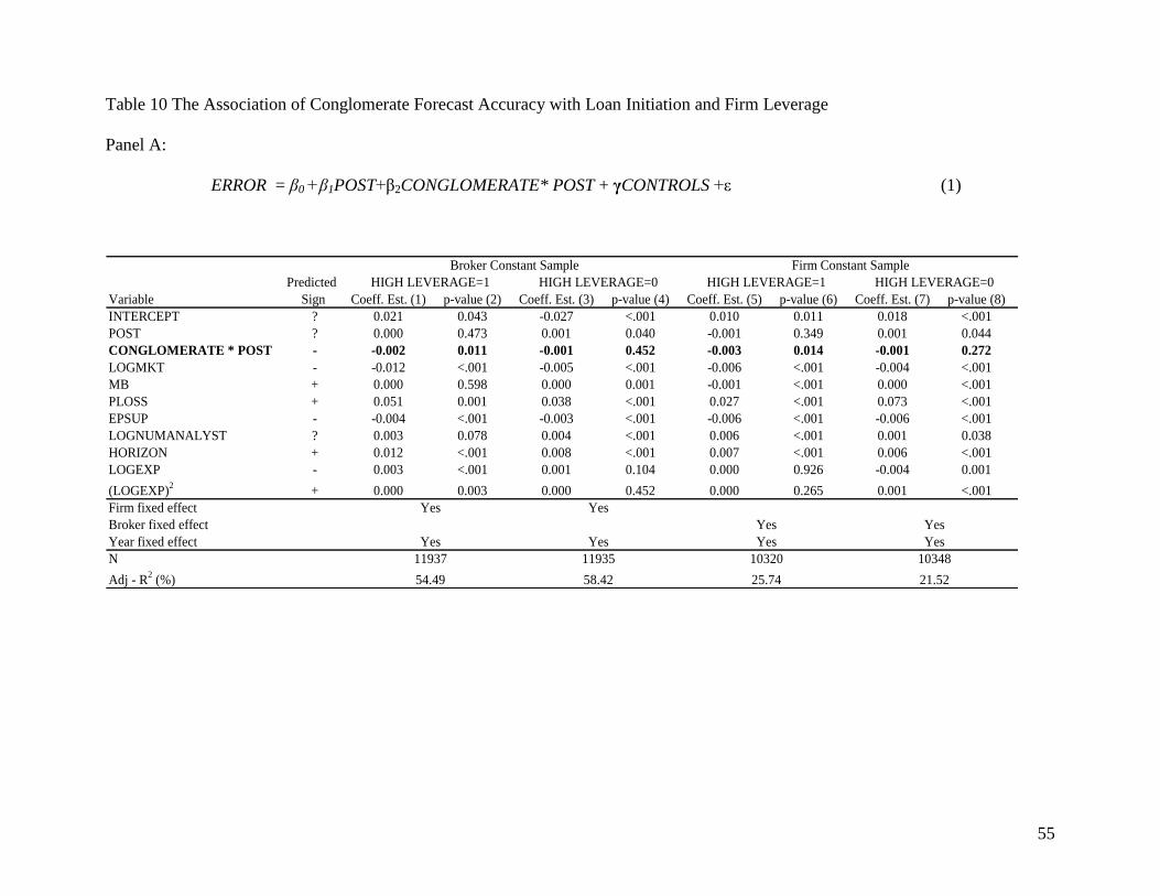
55
Table 10 The Association of Conglomerate Forecast Accuracy with Loan Initiation and Firm Leverage
Panel A:
ERROR = β0 +β1POST+β2CONGLOMERATE* POST + γCONTROLS +ε (1)
Predicted
Variable Sign Coeff. Est. (1) p-value (2) Coeff. Est. (3) p-value (4) Coeff. Est. (5) p-value (6) Coeff. Est. (7) p-value (8)
INTERCEPT ? 0.021 0.043 -0.027 <.001 0.010 0.011 0.018 <.001
POST ? 0.000 0.473 0.001 0.040 -0.001 0.349 0.001 0.044
CONGLOMERATE * POST - -0.002 0.011 -0.001 0.452 -0.003 0.014 -0.001 0.272
LOGMKT - -0.012 <.001 -0.005 <.001 -0.006 <.001 -0.004 <.001
MB + 0.000 0.598 0.000 0.001 -0.001 <.001 0.000 <.001
PLOSS + 0.051 0.001 0.038 <.001 0.027 <.001 0.073 <.001
EPSUP - -0.004 <.001 -0.003 <.001 -0.006 <.001 -0.006 <.001
LOGNUMANALYST ? 0.003 0.078 0.004 <.001 0.006 <.001 0.001 0.038
HORIZON + 0.012 <.001 0.008 <.001 0.007 <.001 0.006 <.001
LOGEXP - 0.003 <.001 0.001 0.104 0.000 0.926 -0.004 0.001
(LOGEXP)2
+ 0.000 0.003 0.000 0.452 0.000 0.265 0.001 <.001
Firm fixed effect
Broker fixed effect
Year fixed effect
N
Adj - R2 (%)
Yes
Yes
HIGH LEVERAGE=1 HIGH LEVERAGE=0HIGH LEVERAGE=0HIGH LEVERAGE=1
11937 11935
Yes
58.42
Yes
Broker Constant Sample
25.74 21.52
Yes
54.49
Yes
10320 10348
Yes
Firm Constant Sample
Yes

56
Table 10 (To be continued)
Panel B:
ERROR = β0 +β1POST+β2CONGLOMERATE* POST + γCONTROLS +ε (1)
Predicted
Variable Sign Coeff. Est. (1) p-value (2) Coeff. Est. (3) p-value (4) Coeff. Est. (5) p-value (6) Coeff. Est. (7) p-value (8)
INTERCEPT ? -0.026 <.001 -0.007 0.287 0.028 <.001 0.018 <.001
POST ? 0.000 0.358 0.000 0.264 0.000 0.668 0.000 0.166
CONGLOMERATE * POST - -0.003 0.005 -0.001 0.164 -0.004 0.018 0.000 0.660
LOGMKT - -0.008 <.001 -0.001 0.052 -0.006 <.001 -0.002 <.001
MB + 0.000 0.055 0.000 0.631 -0.002 <.001 0.000 0.454
PLOSS + 0.069 <.001 -0.038 0.004 0.017 <.001 0.089 <.001
EPSUP - -0.006 <.001 -0.001 0.015 -0.012 <.001 0.000 0.561
LOGNUMANALYST ? 0.002 0.057 0.001 0.440 0.003 0.029 0.000 0.911
HORIZON + 0.012 <.001 0.007 <.001 0.009 <.001 0.004 <.001
LOGEXP - 0.002 0.004 -0.001 0.148 -0.004 <.001 -0.005 <.001
(LOGEXP)2
+ 0.000 0.020 0.000 0.179 0.001 <.001 0.001 <.001
Firm fixed effect
Broker fixed effect
Year fixed effect
N
Adj - R2 (%)
Firm Constant Sample
Yes
Broker Constant Sample
19.85 31.76
Yes
55.22
Yes
10253 10415
Yes Yes
14971 8901
Yes
43.49
Yes
Yes
INVEST=0 INVEST=1INVEST=1INVEST=0
Table 10 Panel A presents results of testing the relation between conglomerate analyst forecast accuracy and loan initiation for
borrowers with high leverage and borrowers with low leverage based on the broker-constant sample and the firm-constant sample,
respectively. HIGHLEVERAGE is a dummy variable coded as 1 if the borrower's leverage ratio (measured as total debt (Compustat
#34 + #9) scaled by total assets (Compustat #6)) is above the sample median, and 0 otherwise. Panel B presents results for borrowers
with an investment grade rating and borrowers without an investment grade rating, respectively based on two samples. A credit rating
equal or above BBB is defined as investment grade rating. In the broker-constant sample, a loan deal for the borrower is assigned for
their matching non-borrowers hypothetically, which assume the same loan initiation date. Firm and year fixed effects are included in
the model for the broker-constant sample and broker and year fixed effects are included in the model for the firm-constant sample.
Robust standard errors clustered at the firm level are used to derive p values. All variables are defined in Appendix B.

57
Appendix A
Panel A: List of Conglomerate banks and their Securities Subsidiaries
Financial conglomerate (Bank) Security subsidiaries
ABN ABN AMRO Inc.
Bank of America Banc of America
Bank of Montreal BMOCM-Canada
Bank of Montreal BMOCM-US
Bank of Nova Scotia Scotia Capital
CIBC CIBC World Mkts
Capital One Bank Capital One
Citigroup Citigroup
Commerzbank Commerzbank
Credit Agricole Calyon Sec. USA
Credit Suisse Group Credit Suisse Securities (USA), LLC
Deutsche Bank DeutscheBankSec
Dresdner Dresdner US
FRB FBR & Company
Fortis Fortis Sec.
HSBC HSBC
JP Morgan J.P.Morgan
KeyBank NA KeyBanc Capital
National Bank of Canada NB Financial
National City Bank NatCity Inv.
U.S. Bankcorp Piper Jaffray
Regions Financial Group Morgan Keegan
Royal Bank of Canada RBC Capital Mkt
Royal Bank of Canada RBC Wealth Mgmt
SunTrust SunTrust RH
Toronto Dominion Commerce Cap
Toronto Dominion TD Newcrest
UBS AG UBS (US)
UBS AG UBS Canada
Wachovia A.G. Edwards
Wachovia Wachovia Cap
Wells fargo Ragen Mackenzie

58
Appendix A (Continued)
Panel B: Conglomerate banks in the broker and firm constant samples
N % N %
ABN 3 0.72 2 0.53
Bank of America 120 28.71 106 28.19
Bank of Montreal 2 0.48 2 0.53
Bank of Nova Scotia 1 0.24 1 0.27
CIBC 3 0.72 3 0.72
Capital One Bank 1 0.24 1 0.27
Citigroup 89 21.29 70 18.62
Credit Suisse 10 2.39 10 2.66
Deutsche Bank 15 3.59 14 3.72
HSBC 1 0.24 1 0.27
JP Morgan 106 25.36 106 28.19
Regions Financial Group 1 0.24 1 0.27
Royal Bank of Canada 1 0.24 1 0.27
SunTrust 20 4.78 19 5.05
UBS AG 4 0.96 3 0.8
Wachovia 41 9.81 36 9.57
Total 418 100 376 100
Panel C: Lender role in the broker and firm constant samples
Lender role Broker Constant Sample Firm Constant Sample
N % N %
Admin agent 263 62.92 240 63.83
Agent 45 10.77 43 11.44
Arranger 8 1.91 7 1.86
Bookrunner 2 0.48 1 0.27
Documentation agent 6 1.44 6 1.6
Lead manager 1 0.24 1 0.27
Mandated arranger 1 0.24 1 0.27
Syndications agent 92 22.01 77 20.48
Total 418 100 376 100 Appendix A Panel A reports the list of financial conglomerates contained in Dealscan
with the left column being bank holding company and the right column being the broker
division. Panel B describes the frequency distribution of financial conglomerates for all
loan deals in our broker-constant sample and firm-constant sample, respectively. Panel C
reports the frequency distribution of the role of lead arranges for all loan deals in our
broker-constant sample and firm-constant sample, respectively.

59
Appendix B: Variable Definition
Dependent variables:
ERROR = analyst forecast error, calculated as |annual EPS forecast – actual
EPS forecast|/price, where price is firm stock price at the beginning
of forecast month.
Independent variables:
CONGLOMERATE = 1 if an EPS forecast is issued by a bank-affiliated analyst,
and 0 otherwise.
POST = 1 if an EPS forecast is issued after loan initiation, and 0
otherwise.
MKT = market value of equity (Compustat #199 * #25) measured at the
end of the fiscal year prior to an EPS forecast.
SMALLFI RM = dummy variable coded as 1 if LOGMKT is below the sample
median, and 0 otherwise .
ASSET = total assets (Compustat #6).
MB = market value of equity divided by book value of equity (Compustat
#60) measured at the end of the fiscal year prior to an EPS forecast.
PLOSS = the probability of a firm experiencing loss in the fiscal year prior to
an EPS forecast is issued. The probability is predicted using the
model with industry fixed effects and industry is based on three
digit SIC code as follows:
Prob (loss = 1) = Industry fixed effects + γ1LOGMKT
+ γ2 LAG_ROA + γ3 LAG_CFO + γ4CFO + γ6SG
+ γ7DIVDUM+ ε
Where LOGMKT is natural logarithm of market value of equity,
LAGROA is returns on assets (Compustat #18/#6) at the end of
prior fiscal year; LAG_CFO and CFO is operating cash flow
scaled by total assets (Compustat #308/#6) measured at the end of
prior fiscal year and the end of current fiscal year, respectively; SG
is sales growth (Compustat Δ#12/#12); and DIVDUM is dummy
variable equal to 1 if a firm pays dividend, and 0 otherwise.
EPSUP = 1 if a firm experiences an increase in EPS compared with previous
fiscal year, and 0 otherwise measured at the end of the fiscal year
prior to an EPS forecast..

60
NUMANALYST = average number of analysts following a firm over the course of a
fiscal year measured during the fiscal year prior to an EPS forecast.
Natural logarithm is taken in the regression.
STD DEV = the average of standard deviation of analyst annual EPS forecast
over the course of a fiscal year measured during the fiscal year
prior to an EPS forecast.
HIGH STDDEV = dummy variable coded as 1 if STD DEV is above the sample
median, and 0 otherwise.
HORIZON = number of days between the time when an EPS forecast is issued
and the actual EPS announcement date. Natural logarithm is taken
in the regression.
EXPERIENCE = number of months between the time when an analyst started to
follow a firm and the time when a specific forecast is issued in
year t. Natural logarithm is taken in the regression.
LEVERAGE = total debt (Compustat #34 + #9) scaled by total assets (Compustat
#6).
HIGHLEVERAGE = dummy variable coded as 1 if LEVERAGE is above the sample
median and 0 otherwise.
BADNEWS = dummy variable coded as 1 if cumulative abnormal return in the
year that an EPS forecast is issued. is negative, and 0 otherwise.
INVEST = dummy variable coded as 1 if a firm has a S&P credit rating equal
or above BBB, and 0 otherwise.
BANK SHARE = ownership of a loan by a lead arranger.
FINCOVENANT = dummy variable coded as 1 if a deal contains at least one financial
covenant, and 0 otherwise.