Do Basketball Scoring Patterns Reflect Illegal Point

Shaving or Optimal In-Game Adjustments?∗

Jesse Gregory

University of Wisconsin, NBER

jmgregory@ssc.wisc.edu

Current Version: August, 2017

Abstract

This paper develops and estimates a model of college basketball teams’ search for scoringopportunities, to provide a benchmark of the winning margin distributions that should arise ifteams’ only goal is to win. I estimate the model’s structural parameters using first-half play-by-play data from college games and simulate the estimated model’s predicted winning margindistributions. Teams’ optimal state-dependent strategies generate patterns that match thosepreviously cited as evidence of point shaving. The results suggest that corruption in NCAAbasketball is less prevalent than previously suggested and that indirect forensic economicsmethodology can be sensitive to seemingly innocuous institutional features.JEL Codes: C61, L83 K42

∗I am grateful to John Bound, Charlie Brown, Morris Davis, Robert Gillezeau, Sam Gregory, Dmitry Lubensky,Brian McCall, Mike McWilliams, Todd Pugatch, Colin Raymond, Lones Smith, Chris Taber, Justin Wolfers, and EricZitzewitz for helpful comments. All remaining errors are my own.

Measuring corruption is inherently difficult because law-breakers cover their tracks. For thatreason, empirical studies in forensic economics typically develop indirect tests for the presence ofcorruption. These tests look for behavior that is a rational response to incentives that only thosewho engage in the particular corrupt behavior face. The validity of these indirect tests depends crit-ically on the assumption that similar patterns do not occur if agents only respond to the incentivesgenerated by the institutions that govern non-corrupt behavior.

Research designs in forensic economics vary to the extent that they are informed by formaleconomic theory. In a survey of the field, Zitzewitz (2011) proposes a “taxonomy” of forensiceconomic research designs that ranges from the entirely atheoretical, in which corrupt behavior ismeasured directly, to the formally theoretical, in which corrupt behavior is inferred from particularviolations of price theory or the efficient-market hypothesis. A common intermediate approach isto posit a statistical model of non-corrupt behavior and to measure the extent to which observedbehaviors deviate from that model in a manner that is consistent with corrupt incentives. Thesoundness of a research design of this variety depends on the plausibility of the assumed statisticalmodel and the extent to which the study’s findings are robust to deviations from the assumedstatistical model.

A recent application of this “intermediate” forensic economic strategy purports to find evidenceof rampant illegal point shaving in college basketball (Wolfers 2006). Point shaving is when aplayer on a favored team places a point-spread bet that the opposing team will “cover” the pointspread – win outright or lose by less than the point spread – and then manages his effort so that histeam wins but by less than the point spread.1 Because this behavior causes some games that wouldotherwise end with the favored team winning by more than the median winning margin to win byjust below the median winning margin, point shaving tends to increase the degree of right skewnessin the distribution of favored teams’ winning margins. Under an assumption that the distributionof winning margins would be symmetric in the absence of point shaving, Wolfers (2006) tests forpoint shaving by measuring skewness in the empirical distribution of winning margins around thepoint spread. The skewness-based test suggests that point shaving is rampant, occuring in about sixpercent of games where one team is strongly favored. Wolfers’ study garnered significant attentionin the popular media2, reflecting public surprise that corruption might be so pervasive in amateurathletics. While point-shaving scandals have been uncovered with some regularity dating as farback as the early 1950s, the public’s perception seems to be that such scandals are fairly isolated

1A point-spread bet allows a gambler to wager that a favored team’s winning margin will exceed a given number,the point spread, or bet that the winning margin will not exceed the point spread. A typical arrangement is for thebettor to risk $11 to win $10 for a point spread bet on either the favorite or the underdog.

2Bernhardt and Heston (2008) cite a group of media outlets in which Wolfers’ (2006) study was featured. Theseinclude the “New York Times, Chicago Tribune, USAToday, Sports Illustrated and Barrons, as well as National PublicRadio and CNBC TV.”

1

incidents.To obtain a more formal benchmark of the patterns that one should expect under the no-point-

shaving null hypothesis, this paper develops and estimates a dynamic model of college basketballteams’ within-game searches for scoring opportunities. Using play-by-play data from the firsthalves of NCAA games linked to gambling point spread data, I estimate the model’s structural pa-rameters from play during the first halves of games. With the estimated model, I then simulate playduring the second halves of games. I find that the sorts of strategic adjustments across game states(current score and time remaining) that are commonly observed in actual games are consistent withan optimal policy. Further, I find that the scoring patterns generated by optimal policies generateskewness patterns that closely match those previously cited as evidence of illegal point shaving.The analysis suggests that the existing skewness-based test greatly exaggerates the prevalence ofpoint shaving.

In the model, teams take turns as the offensive side searching for scoring opportunities. Theoffensive side faces a sequence of arriving shot opportunities which vary in their probability ofsuccess. As in actual NCAA basketball games, the offensive side has 35 seconds to attempt a shotbefore the opponent is automatically awarded the ball. Like a worker in a job-search model, thesearching team compares each arriving opportunity with the value of continued search. Becauseof the fixed horizon, the optimal strategy within a possession is a declining reservation policywhere initially only the most advantageous opportunities are accepted and less advantageous op-portunities become acceptable as time goes by. The optimal reservation policy depends on thecurrent relative score and the time remaining in the game. Especially near the end of the game, atrailing team prefers to hurry by taking short possessions, and the leading team prefers to stall bytaking long possessions. I show that the direction of skewness that this process introduces to thedistribution of the stronger team’s winning margin depends on whether stalling incurs the largeropportunity cost (causing left skewness) or hurrying incurs the larger opportunity cost (causingright skewness). The parameters of the search process determine the opportunity cost of stallingand the opportunity cost of hurrying.

I estimate the model’s parameters using play-by-play data from the first halves of games, andI find that under the estimated parameter values stalling is less costly than hurrying. As a result,the leading team makes larger strategic adjustments than the trailing team, and the score differencetends to shrink (or grow more slowly) on average compared to what would occur if each team chosethe strategy that maximized its expected points per possession. These optimal adjustments resultin a right-skewed distribution of winning margins in games in which one team is a large favorite.As a false experiment, I apply the skewness-based test for point shaving to simulated data. I find“evidence” of point shaving in the two highest point-spread categories, and the implied prevalence

2

of point shaving is statistically indistinguishable the Wolfers (2006) estimate.3

Studies in economics that treat sports as a research laboratory are sometimes criticized as beingunlikely to generalize to more typical economic settings. However, for forensic economics, studiesinvolving sports have provided particularly compelling case studies. Participants’ willingness toengage in illegal behavior in the highly monitored environment of sports competitions suggests thatcorruption likely plays a more prominent role in less well-monitored settings (Duggan and Levitt,2002; Wolfers, 2006; Price and Wolfers, 2010; Parsons, Sulaeman, Yates, and Hamermesh, 2011).The high-quality data and well-defined rules and institutions that are perhaps unique to sports alsoprovide an excellent opportunity to assess the robustness of forensic economic methodology. Thisstudy’s findings suggest that forensic economic studies should take great care to assess the robust-ness of their methods to unmodelled assumptions about even seemingly innocuous institutionalfeatures. Further, the findings suggests that structural modeling can yield improved predictionsof behavior under the no-corruption null hypothesis even in settings in which off-the-shelf pricetheory and efficient market theory do not yield immediate predictions.

The conclusions of this paper conform with those of Bernhardt and Heston (2008). Bernhardtand Heston find that the patterns attributed to point shaving by Wolfers (2006) are present in subsetsof basketball games in which gambling related malfeasance is less likely on prior grounds. Theauthors conclude that even in the absence of point shaving, asymmetries exist in the distributionof the final-score differentials among games in which one team is a large favorite4. Because theapproach of this paper and the purely empirical approach of Bernhardt and Heston (2008) arevulnerable to different criticisms, I consider my study a complement to their work.

The remainder of the paper is organized as follows: Section 1 develops a simple illustrativemodel, Section 2 develops a richer model of the basketball scoring environment, Section 3 de-scribes estimation, Section 4 describes the data, Section 5 presents point estimates of the model’sstructural parameters and examines the model’s fit, Section 6 presents the results of simulations cal-ibrated with estimated parameters, Section 7 provides corroborating evidence for the main model-based results, and Section 8 concludes.

3It should be noted that Wolfers’ (2006) article acknowledges the limitations of the skewness-based test relativeto a test more formally grounded in theory, and characterizes the resulting estimates as “prima facie” evidence ofwidespread point shaving. The structural approach that Wolfers’ article outlines as a possible extension differs fromthe approach in this study. Wolfers suggests that a structural model of the point shaver’s behavior might allow for amore accurate inference about the prevalence of point shaving based on the observed deviation from symmetry in theempirical distribution. This study adopts a structural approach to more accurately characterize the distribution onemight expect under the no-point-shaving null.

4Bernhardt and Heston (2008) suggest that the goal of maximizing the probability of winning could induce anasymmetric final-score distribution, but stop short of suggesting a theoretical model.

3

1 Illustrative Two-Stage Dynamic Game

Before turning to the full dynamic model, I use a simple two-stage model to illustrate the kindsof model primitives that can rationalize a skewed distribution of winning margins in a dynamiccompetition.

In this simple model, two competitors A and B accumulate points during a two stage game.Let X1 represent the difference between A’s and B’s points during stage 1, and let X2 representthe difference between A’s and B’s points during stage 2. Following stage 2, A receives a payoffof one if X1 + X2 ≥ 0 and zero otherwise, and B receives a payoff of one if X1 + X2 < 0 andzero otherwise.

A random component influences the scoring process. Before each stage, A and B each selectan action that influences the mean and the variance of scoring during that stage. Before stage 1, Aselects σA1 ∈ [0, 1] and B selects σB1 ∈ [0, 1]. Stage 1 then occurs, and both competitors observethe realized value of X1. Then before stage 2, A selects σA2 ∈ [0, 1] and B selects σB2 ∈ [0, 1].The quantities X1 and X2 are given by,

X1 = µ(σA1)− µ(σB1) +(σA1 + σB1

)Z1 + ∆ (1)

X2 = µ(σA2)− µ(σB2) +(σA2 + σB2

)Z2 + ∆ (2)

where µ() is a twice differentiable real-valued function that describes the relationship between aplayers chosen action and the mean of scoring, Z1 and Z2 are standard normal random variablesthat are independent from one another, and ∆ ≥ 0 is a constant that allows for the possibilitythat A is stronger than B. I assume that µ() is bounded, strictly concave, and reaches an interiormaximum on [0, 1]. The choice of a very high variance (σ near one) or a very low variance (σnear zero) involves a lower expected value of scoring. To ensure an interior solution, I assume thatthe µ′(σ) is unbounded, going to −∞ as σ approaches 1 and going to∞ as σ approaches 0 (Anexample of a function satisfying these assumptions is a downward-facing semi-circle).

Because each competitor maximizes a continuous function on a compact set, the minimaxtheorem ensures that a solution to this zero-sum game exists, and inspection of the players’ bestreply-functions finds that the solution is unique. The optimal stage 2 actions (σ∗A2, σ

∗B2) satisfy the

first order condition,

µ′(σ∗A2) =X1 + µ(σ∗A2)− µ(σ∗B2) + ∆

σ∗A2 + σ∗B2

= −µ′(σ∗B2) (3)

4

Figure 1 plots A’s iso-payoff curves along with the choice set µ() to illustrate the reasoning behindthis result. The vertical axis plots the expected final score entering stage 2. The horizontal axisplots the standard deviation of the stage 2 score differential. A’s win probability depends on theratio of the expected final score differential to the standard deviation of stage 2 scoring, so theIso-payoff curves are rays away from the origin.5 Proportional increases in the expected final scoredifferential and in the standard deviation of stage 2 scoring do not affect win probabilities. IfX1 + ∆ = 0, A and B (depicted by the iso-payoff ray extending horizontally from the origin)each have an equal chance of winning heading into stage 2, and each chooses the strategy thatmaximizes its expected points. If X1 + ∆ > 0, A’s chance of winning is greater than 1/2, andA’s optimal strategy is to select a relatively low-variance action in order to reduce the chances ofa come from behind win for B. If X1 + ∆ < 0, A’s chance of winning is less than 1/2, and Aselects a relatively high-variance action in order to increase its chances of a come from behindwin. These optimal choices are characterized by the tangency of the mean-variance choice set µ()

to the state-dependent iso-payoff curves, with this result occurring because A’s iso-payoff curveis downward sloping when its win probability is below 1/2 and is upward sloping when its winprobability is above 1/2.

In stage 1, A andB each have a unique optimal strategy. Define V (X1) to beA’s expected pay-off entering stage 2 if the relative score after stage 1 is X1. The optimal stage 1 actions (σ∗A1, σ

∗B1)

are the solution to,

maxσA1

minσB1

∫ ∞−∞

V(µ(σA1)− µ(σB1) + ∆ +

(σA1 + σB1

)z)dΦ(z) (4)

where Φ() is the standard normal CDF.Now consider how the players’ optimal strategies influence the shape of the distribution of winningmargins. One might expect for the winning margin X to be symmetrically, because X = X1 +X2

is the sum of two normally distributed random variables. That is not the case in general, because theplayers’ choices introduce dependence betweenX1 andX2. In two particular cases, the distributionof X is symmetric. The first case relies on the symmetry of the game when A and B are evenlymatched.

Proposition 1: The winning margin is symmetric when A and B are evenly matched: Assume

that ∆ = 0, which means that the two teams are evenly matched. Then the distribution of winning

margins is symmetric.6

5Spcifically, A’s win probability is Φ(X1 + µ(σ∗A2)− µ(σ∗B2) + ∆

σ∗A2 + σ∗B2

), where Φ() is the standard normal CDF.

6This result follows directly from the symmetry of the game. Because the solution is unique, switching the names

5

Figure 1: The Optimal Choice of a Mean-Variance Pair During Stage 2 of the Stylized Model

Choose a low variance when leading

Choose a high variance when trailing

X1

+ E(X2

|X1

)

σA2

+ σB2

X1,high

+ μ(σA2

) - μ*(σB2

) + Δ

X1,low

+μ(σA2

) - μ*(σB2

) + Δ

Iso-payoff curves

Note: Taking B’s strategy as given, A faces a choice among combinations of the mean and the variance of the finalscore. Two example choice sets are provided, one corresponding toA trailing after stage 1 and the other correspondingto A leading after stage 1. Iso-expected payoff curves are represented by dashed lines. Because X2, the score duringstage 2, is normally distributed, A’s probability of winning depends on the ratio of the expected value of the final scoreto the standard deviation of X2. As such, the iso-expected payoff curves are rays away from the origin.

6

Symmetry also holds when A and B are not evenly matched if the menu function µ() is sym-metric. In that case A’s and B’s strategic adjustments, based on the realized value of X1, haveexactly offsetting impacts on the mean and the variance of X2.

Proposition 2: The winning margin is symmetric (normally distributed) when increasingvariance and decreasing variance are equally “costly”: Assume that µ() is symmetric, that is,

that µ′(.5) = 0 and that µ(.5+c) = µ(.5−c) for any c ∈ [0, .5]. Then, E(X1) = E(X2|X1) = ∆,

σA1 + σB1 = σA2 + σB2 = 1, and X ∼ N(2∆, 2). Proof provided in Appendix 1.

When µ() is symmetric, E(X2|X1) is constant. In general, though, E(X2|X1) is not constant,and dependence between X1 and X2 can generate skewness in the sum of X1 and X2. Proposition3 provides conditions under which E(X2|X1) monotonically increases or decreases in X1.

Proposition 3: The monotonicity ofE(X2|X1) if strategic adjustment of the variance is moredifficult in one direction than the other: Let σ∗ be the action that maximizes µ(). Assume that for

any σ′ < σ∗ and σ′′ > σ∗ with u′(σ′) = −u′(σ) that |u′′(σ′)| < |u′′(σ′′)| (a player who prefers

to increase variance faces a steeper marginal cost than a player who prefers to reduce variance).

Then E(X2|X1) monotonically decreases in X1. Conversely, assume that for any σ′ < σ∗ and

σ′′ > σ∗ with u′(σ′) = −u′(σ) that |u′′(σ′)| > |u′′(σ′′)| (a player who prefers to reduce variance

faces a steeper marginal cost than a player who prefers to increase variance). Then E(X2|X1)

monotonically increases in X1. Proof provided in Appendix 1.

The results thus far characterize the slope of the expected second-half scoring “drift”E(X2|X1)

with respect to X1. Proposition 4 suggests that the direction of skewness in the winning margindistribution depends on the curvature of E(X2|X1) in X1.

Proposition 4: A sufficient condition for determining the direction of skewness in winning mar-gins: Assume that E(X2|X1) is convex in X1. Then the winning margin is right skewed. Con-

versely, assume that E(X2|X1) is concave in X1. Then the winning margin is left skewed. Proof:An application of Zwet (1964). See Appendix 1 for more details.

Because the function µ() is bounded, E(X2|X1) is also bounded and, therefore, may not beconvex or concave over all values of X1. Nonetheless, propositions 3 and 4 together with theboundedness of E(X2|X1) suggest circumstances under which one might expect to find skewnessin the distribution of winning margins. Figure 2 illustrates this idea. When ∆ is large, X1 willtypically be large. If E(X2|X1) monotonically decreases in X1 but is bounded, one might expectE(X2|X1) to be convex over many large values of X1. In that case, one would expect the dis-tribution of winning margins in games with large ∆ to be right skewed. Similarly, if E(X2|X1)

of A and B cannot change the distribution of winning margins.

7

monotonically increases in X1 but is bounded, one might expect E(X2|X1) to be concave overmany large values of X1. In that case, one would expect the distribution of winning margins ingames with large ∆ to be left skewed.

Wolfers’ (2006) statistical test attributes right skewness in the distribution of the favorite’swinning margins to the influence of point shaving. If winning margins are right skewed in theabsence of point shaving, then that test overstates the true prevalence of point shaving. On theother hand, if winning margins are left skewed in the absence of point shaving, then that testunderstates the true prevalence of point shaving.

The remainder of the paper considers a model of basketball teams’ search for scoring oppor-tunities in order to assess whether a skewed distribution of winning margins is consistent withoptimal strategies. In basketball games, the two teams alternate turns as the offensive side, and thegame ends after a fixed amount of time has passed. The total number of possessions that occurs hasa significant influence on the variance of the score. During a given possession, a team can reducethe variance of the scoring that will occur during the remainder of the game by stalling; that is,taking a lot of time before attempting a shot. A team can increase the variance of the scoring thatwill occur during the remainder of the game by hurrying; that is, attempting a shot very quickly.

The reasoning behind this simple model suggests that the favored team’s winning marginshould be right skewed if increasing the variance of points has a lower opportunity cost than re-ducing the variance of points. In the context of the richer model that I consider, that condition issatisfied when stalling has a lower opportunity cost than hurrying. The estimated model finds that,indeed, the opportunity cost to stalling is lower than the opportunity cost of hurrying in NCAAbasketball games. Further, the simulations that I conduct using the estimated model suggest thatteams’ optimal end-of-game adjustments generate skewness patterns that closely resemble thosepreviously attributed to point shaving.

2 Full Model

2.1 Model

In this section, I propose a more detailed model of the environment in which basketball teamscompete. Teams alternate turns as the offensive side, and the team that is on offense faces asequence of arriving shot opportunities that vary stochastically in quality. I refer to a single turnas the offensive side as a possession. The team that is searching for a scoring opportunity mustcompare the potential reward of each opportunity with the option value of continued search. Assuch, I model the game as a sequence of many alternating periods of finite horizon search.

In this model, the tradeoff between the expected value of points and the variance of points

8

Figure 2: State Dependent Strategies Can Skew Winning Margins in Either Direction

E(X2|X1)

XHalftime Lead: X10

Expected 2nd HalfScoring Drift:

(a) Drift when low-variance strategy (stalling) is lesscostly

E(X2|X1)

XHalftime Lead: X10

Expected 2nd HalfScoring Drift:

(b) Drift when high-variance strategy (hurrying) is lesscostly

X1X1+E(X2|X1) 0

fX1+E(X2|X1)

Exp. Final Winning Margin: , Halftime Lead:

Density

(c) Drift being convex in score→ right skewness

fX1+E(X2|X1)

X1X1+E(X2|X1) 0

Exp. Final Winning Margin: , Halftime Lead:

Density

(d) Drift being concave in score→ left skewness

Note: Panels (a) and (b) illustrate the average change in the relative score in the second half as a function of thehalftime score in the illustrative two stage model. Panel (a) gives an example second-half scoring drift pattern wherethe drift declines with the favorite’s halftime lead, a pattern that occurs in the illustrative two stage model whenadjusting to a low variance strategy incurs a lower marginal cost than adjusting to a high variance strategy. Panel (b)gives an example second-half scoring drift pattern where the drift increases with the favorite’s halftime lead, a patternthat occurs when adjusting to a low variance strategy incurs a higher marginal cost than adjusting to a high variancestrategy. Panels (c) and (d) illustrates the effect of second half play on the shape of scoring distribution in these twocases. Figure (c) shows that when second half scoring drift is a convex function of the halftime lead over the supportof the halftime lead distribution, as in the right portion of figure (a), second half play introduces right skewness to thewinning margin distribution. Figure (d) shows that when second half scoring drift is a concave function of the halftimelead, as in the right portion of figure (b), second half play introduces left skewness to the winning margin distribution.

9

is endogenous. A unique reservation policy exists that maximizes a team’s expected points perpossession. If the team chooses to hurry, by selecting a lower reservation policy, its expectedpoints per possession will be lower. Also if it stalls by choosing a very high reservation policy,its expected points will be lower. The duration of a given possession influences the variance inthe score in the remainder of the game through its influence on the total number of possessionsthat will occur. Hence, as in the simple model, an opportunity cost is associated with choosing astrategy that substantially raises or substantially reduces the variance of points.

In this more complex model, the team that is on defense is given the opportunity to intentionallyfoul the offensive team. I include this feature because the strategy is ubiquitous in the final minutesof actual NCAA basketball games, and the strategy influences the distribution of winning marginsin a way that the simulation experiments I conduct find to be important.

In the model, two teams,A andB, accumulate points during a single competition with a typicalduration of T seconds. In NCAA basketball games, T = 2400 seconds (40 minutes). If the scoreis not tied at time T , then the game ends. If the score is tied at time T , then play is repeatedlyextended by an additional 300 seconds (five minutes) until a winner is determined. Two measuresof time are relevant. Let t ∈ [0, 1, 2, .., T ] measure the time since the game began in discreteperiods of one second each. At any t, let s ≥ 0 describe the number of seconds since the currentpossession began. The variable s corresponds to the “shot clock” in NCAA basketball games.

One team at a time is on offense searching for a scoring opportunity. Let o ∈ A,B indicatethe team that is on offense. The team that is on offense faces a sequence of scoring opportunities.A scoring opportunity is characterized by a pair of variables, p and π. The variable p ∈ [0, 1]

describes the probability with which an opportunity will succeed if it is accepted. The variableπ ∈ 1, 2, 3 describes the number of points that will be awarded if the opportunity is acceptedand succeeds. For standard opportunities, π ∈ 2, 3, and the particular case when π = 1 isdescribed below.

Each period, time t increases by one. The team on offense switches if one of three eventsoccurs; the team on offense accepts a scoring opportunity at t − 1, the possession duration s

reaches a maximum limit or 35 seconds at t−1 (known as a shot clock violation), or an exogenousturnover occurs between period t− 1 and t. The arrival process for turnovers is described later. Ifthe offensive team does not switch from one period to the next, s increases by one. Otherwise, s isreset to zero.

The variable X = XA − XB measures the difference in the two teams’ accumulated pointtotals. When a team accepts a shot opportunity, the uncertainty is resolved and the offensive teamreceives either 0 or π points.

Scoring opportunities and turnovers arrive stochastically. I impose that no turnovers or shotopportunities arrive during the first five seconds of the possession to reflect the time required in

10

actual games for the offensive team to move the ball from its defensive portion of the court toits offensive portion. Following this initial five-second span, one scoring opportunity arrives eachsecond7. The variables that describe a scoring opportunity are drawn from the conditional densityfunction f(p, π|t, s,X, o). I impose the simplifying assumption that the distribution from whichp and π are drawn depends only on the team that is offense but does not otherwise vary. Thatis f(p, π|t, s,X, o) = f(p, π|o). I also assume that draws of (p, π) are independent across time.Finally, I assume that turnovers arrive with a constant probability for each team, and I let υA and υBdenote the turnover probabilities when the team on offense is A or B. I refer to these assumptionsjointly as a conditional independence assumption (CIA).8 These assumptions facilitate estimationof the model and allow me to conduct simulations of end-of-game play using parameters estimatedfrom data on play early in games.

Both the offense and the defense face a choice during each one-second increment. If noturnover occurs, the team on defense has the option to intentionally foul the team on offense.The defense’s choice of whether to foul or not occurs before realizations of the draw of (p, π).When an intentional foul is committed, the offense is granted two one-point (π = 1) scoring op-portunities during the same period known as free throws. Free throws succeed with known (to theteams) probabilities pftA and pftB . If no turnover occurs and the defense chooses not to intentionallyfoul, a shot opportunity (p, π) is drawn. The offense must choose whether to accept the currentopportunity or to continue searching. I denote the choice spaces of the defense and offense withAD = 0, 1 and AO = 0, 1. For the team on defense, 1 represents the choice to intentionallyfoul. For the team on offense, 1 represents the choice to accept a scoring opportunity.

When the game ends, the teams receive payoffs UA and UB. The team with the higher scorereceives a payoff of one and the team with the lower score receives a payoff of zero.910 Because

7The assumption that a scoring opportunity arrives every second is not as restrictive as it might seem, becausethe arrival of a very poor scoring opportunity (one that succeeds with very low probability) is no different from anon-opportunity.

8This assumption implies that teams’ turnover hazards and arriving shot quality distributions are constant withinpossessions (over the course of the shot clock) and across possessions (by time-by-score game states). These assump-tions may be violated to some extent within actual games if teams adopt tactics that trade off turnover hazard againstshot quality (a risk/reward trade-off) or choose to remove star players from the game when the score differential be-comes large. I discuss the potential consequences of these sorts of model failures below, arguing that if anything theyare likely to exacerbate any right-skewness in the distribution of favored teams’ winning margins.

9One deviation from this payoff function would be if teams place some utility weight on the final score differentialin addition to a discrete preference for winning over losing. This would be rational if, for instance, selection intopostseason tournaments is awarded based partially on winning margins in addition to teams’ simple win/loss records.If teams do have payoff functions that place weight on score differential, optimal end of game strategies would tend tobe closer to those that maximize points per possession than those predicted by this model, and would thus generate lessskewed winning margins distributions than those predicted by this model. This is apparent by considering the extremecase where teams only place weight on score differential (and place no additional weight on winning), in which casewinning margins will be approximately symmetric as teams would simply maximize expected points per possessionthroughout the game.

10Another deviation from this payoff function would be if teams place disproportionate weight on some of their

11

the model is used to benchmark the patterns one should expect in the absence of corruption, teams’only objective is to win the game. Each team chooses its strategy to maximize its expected payoff.Denote the vector of state variables with ω = t, s,X, o, p, π, and let Ω = ω denote the statespace. Define the value function V A(ω) = E(UA|ω) to be A’s expected payoff from the state ω.Because the game is zero-sum, this value function also characterizes B’s expected payoff. Theuniqueness of this expected payoff function follows directly from the uniqueness of the teams’reservation policies.

By CIA and the assumed process for the state transitions, state transitions are Markovian. Thatproperty allows the optimization to be expressed as the following dynamic programming problem.

V A(ω) = maxa∈AA(ω)

min

b∈AB(ω)

E[V A(ω′)|ω, a, b]

(5)

The sets AA(ω) and AB(ω) represent the teams’ choice sets given the current state. A team’schoice set is AO if ω indicates that the team is on offense and is AD otherwise.

2.2 Approximate Model Solution

The model developed in the previous section does not have an analytic solution. However, forany parameterization of the density function f , a numerical solution can be computed using back-ward induction. I compute the full numerical solution to the model when performing dynamicsimulations in section 6. In this section, however, I develop an approximate solution method thatdescribes the optimal policy within a single possession. I use this approximate solution as the basisfor estimating the model’s parameters. There are several advantages to this approach. Most im-portantly, the approach ensures that the model’s parameters are identified by teams’ choices within

possessions during the portion of games where pace adjustments are not important, as opposed tobeing identified by teams’ end-of-game adjustments, which may or may not be contaminated bypoint shaving incentives. Also, the approach provides significant computational savings because itavoids having to repeatedly solve the full model with backward induction during estimation.

Define the function EV to be A’s expected payoff in a state prior to the realization of theoffensive team’s shot opportunity,

games during the season (e.g. conference games or games against rivals) than others. This could be modeled byproviding teams with 0 vs. 1 payoffs in some games and, say, 0 vs.V (with V > 1) payoffs in other games. Holdingteams’ structural search parameters fixed, these payoff changes would have no effect on teams’ strategies, since theoptimal strategy is still to maximize win percentage. Similarly, even if teams allocate their game-to-game effort overthe course of the season disproportionately to these “high-payoff” games, as long as these incentives are reflected inthe point spread (as Table 4 suggests is the case) the estimated model should capture these effects because the structuralsearch parameters are allowed to depend on the point spread.

12

EV ([t, s,X, o]) = E(p′,π′)

[V(

[t, s,X, o, p′, π′])]

(6)

I now construct a linear approximation of EV within a single possession that begins in the stateω0 = [t, s = 0, X, o]. Let s? denote the duration of the possession, and let x? denote the changein X that occurs as a result of the possession. Then the state of the following the possession isω? = [t + s?, s = 0, X + x?,−o], where −o indicates the opponent of team o. I next note that theexpected payoff in the state ω? can be approximated linearly using,

EVA

(ω?) ≈ EV A(ω0) + EV AX (ω0) x

? + EV At (ω0) s

?

EVA

(ω?) ≈ EV A(ω0) + EV AX (ω0)

(x? + φ(ω?0) s?

)(7)

whereEV AX = EV ([t, s,X+1, o])−EV ([t, s,X, o]),EV A

t = EV ([t+1, s,X, o])−EV ([t, s,X, o]),and φ(ω?0) = EV A

t (ω?0)/EV AX (ω?0). The term φ(ω?0) can be thought of as a marginal rate of substi-

tution between time and points. The partial effect of one second passing on A’s expected payoff isthe same as a φ(ω?0) point change in the relative score.

Now note that because EV A(ω?) is a positive affine transformation of the expression(x? +

φ(ω?0) s?)

, the within-possession policy that maximizes EV A is the same as the policy that maxi-

mizes(x? + φ(ω?0) s?

). Thus, up to a linear approximation of the value function, all strategically

relevant information from the states t and X is embedded in φ(ω?0).The optimal policy for the team on offense is a reservation rule that I denote with R(s;φ). For

each value of s within the possession, the reservation rule describes the point value pπ for whichthe offense is indifferent between accepting the opportunity and opting for continued search. Usingthe linear approximation developed above, it is straightforward to show that when A is on offensethe optimal reservation rule is,

RA(s;φ) = E(x?∣∣∣s? > s

)︸ ︷︷ ︸

points from continued search

+ φ E(s? − s

∣∣∣s? > s)

︸ ︷︷ ︸point-value of continued search time

(8)

That is, the reservation expected-point value for a particular shot is equal to the expected number ofpoints scored later in the possession conditional on continued search (the first term) plus the points-value of the expected passage of time later in the possession conditional on continued search (thesecond term). Early in the game and in other states where φ ≈ 0 this is the policy that maximizesexpected points per possession. The policy sacrifices expected points to lengthen possessions

13

when φ > 0 (i.e. when a team leads late in a game) and sacrifices expected points to shortenpossessions when φ<0 (i.e. when a team trails late in a game). Given the fixed boundary at s = 35,the reservation value can be defined recursively. First, define the auxiliary function zA(s;φ) =

E[s?φ+ x?

∣∣∣s? ≥ s]. I first construct an expression for zA, and then use zA to construct RA.

zA(s;φ) =

35 υA φ + (1− υ)Emax(pπ, 0

)if s = 35

s υA φ + (1− υ)Emax(pπ, zA(s+ 1;φ)

)if s < 35

(9)

RA(s;φ) =

0 if s = 35

(1− υA)[Emax

(pπ, zA(s+ 1;φ)

)− s φ

]if s < 35

(10)

Recall that υ is the hazard of a turnover in each one-second period. The optimal strategy is adeclining reservation policy. An analogous derivation yields the optimal policy for team B.

To illustrate how the optimal policy varies across game states, figure 3 plots the predictedreservation policies in three different game states holding the model parameters constant; one forwhich φ = 0, one in which the φ < 0 (offensive team trails late in game), and one in whichφ > 0 (offensive team leads late in game). The plots are constructed using the search parametersestimated for the favored team in games with a point spread between 0 and 4. When φ = 0, theintermediate reservation policy is implemented. That is the point-maximizing policy. When φ < 0

a lower reservation policy is chosen, which leads to shorter average possessions and fewer pointsper possession than when φ = 0. When φ > 0 a higher reservation policy is chosen, which leadsto longer average possessions and fewer points per possession than when φ = 0.

Below I use simulation experiments to examine the extent to which these sorts of optimal paceadjustments introduce skewness to the distribution of winning margins. There are other types ofin-game adjustments that teams may make in actual basketball games that are not included in thismodel. For example, the offensive team and/or defensive team may adjust their tactics to tradeoff turnover hazard against the quality of arriving shots. If both teams are on the tactical frontierthen adjustments (by the offense or defense) that increase the expected turnover hazard shouldimprove the expected quality of arriving shots conditional on the shot opportunity arriving (“high-risk/high-reward”). Tactical adjustments that reduce the turnover hazard should reduce the qualityof arriving shot opportunities (“low-risk/low-reward”). Similar to understanding the consequencesof pace adjustments on the skewness of winning margins, one would need to understand whetherthe relative cost in terms of expected points per possession is larger for adjustments towards high-risk or low-risk strategies. If adjustments toward low-risk tactics are less costly than adjustmentstoward high-risk tactics, one would expect larger adjustments by leading teams, toward those low-

14

Figure 3: Predicted Reservation Policies Across Game States

0 5 10 15 20 25 30 350

0.5

1

1.5

Possession Duration (seconds)

Exp

ecte

d P

oint

s

φ < 0

φ = 0

φ > 0

Note: Shot opportunities are characterized by a success probability and a point value. The graphed reservation valuesdepict for a single team type (teams favored by 0 to 4 points) the expected success probability times point value abovewhich it is optimal to accept the opportunity. The optimal policy depends on the game state. The top, middle, andbottom lines correspond to game states in which the marginal rate of substitution between time and points (φ) for thefavorite is positive (0.15), zero, and negative (−0.15). When the partial effect of the passing time on a team’s expectedpayoff is higher, the team adopts a higher reservation policy that results in longer average possessions. Source: author’scalculations.

risk strategies, exacerbating the right-skewness of winning margins.11

3 Estimation

I estimate the parameters governing the search process separately for each of six categories definedby the size of the point spread. The first five point-spread categories are each four points wide,and the sixth category includes all games with a point spread above 20. I estimate one set ofparameters describing the favorite’s search process and another set of parameters describing theunderdog’s search process. Favorites and underdogs in the six point-spread categories make uptwelve team types. This approach allows me to conduct separate simulation experiments by point-spread categories.

11While these other sorts of model features are interesting in their own right, I leave the estimation of the “menu”of such adjustments available to teams for future work.

15

Tabl

e1:

Des

crip

tive

Stat

istic

s-P

osse

ssio

ns

Not

e:T

hesa

mpl

eex

clud

espo

sses

sion

sw

itha

dura

tion

offiv

ese

cond

sor

less

and

poss

essi

ons

that

end

with

ade

fens

ive

foul

that

does

notr

esul

tin

free

thro

ws.

Sour

ce:a

utho

r’s

calc

ulat

ions

usin

gpl

ay-b

y-pl

ayda

tafr

omst

atsh

eet.c

omm

erge

dto

poin

t-sp

read

data

from

cove

rs.c

om.

16

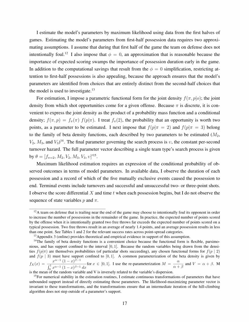
I estimate the model’s parameters by maximum likelihood using data from the first halves ofgames. Estimating the model’s parameters from first-half possession data requires two approxi-mating assumptions. I assume that during that first half of the game the team on defense does notintentionally foul.12 I also impose that φ = 0, an approximation that is reasonable because theimportance of expected scoring swamps the importance of possession duration early in the game.In addition to the computational savings that result from the φ = 0 simplification, restricting at-tention to first-half possessions is also appealing, because the approach ensures that the model’sparameters are identified from choices that are entirely distinct from the second-half choices thatthe model is used to investigate.13

For estimation, I impose a parametric functional form for the joint density f(π, p|o); the jointdensity from which shot opportunities come for a given offense. Because π is discrete, it is con-venient to express the joint density as the product of a probability mass function and a conditionaldensity; f(π, p) = fπ(π) f(p|π). I treat fπ(2), the probability that an opportunity is worth twopoints, as a parameter to be estimated. I next impose that f(p|π = 2) and f(p|π = 3) belongto the family of beta density functions, each described by two parameters to be estimated (M2,V2, M3, and V3)14. The final parameter governing the search process is υ, the constant per-secondturnover hazard. The full parameter vector describing a single team type’s search process is givenby θ = [fπ=2,M2, V2,M3, V3, υ]′15.

Maximum likelihood estimation requires an expression of the conditional probability of ob-served outcomes in terms of model parameters. In available data, I observe the duration of eachpossession and a record of which of the five mutually exclusive events caused the possession toend. Terminal events include turnovers and successful and unsuccessful two- or three-point shots.I observe the score differential X and time t when each possession begins, but I do not observe thesequence of state variables p and π.

12A team on defense that is trailing near the end of the game may choose to intentionally foul its opponent in orderto increase the number of possessions in the remainder of the game. In practice, the expected number of points scoredby the offense when it is intentionally granted two free throws far exceeds the expected number of points scored on atypical possession. Two free throws result in an average of nearly 1.4 points, and an average possession results in lessthan one point. See Tables 1 and 2 for the relevant success rates across point-spread categories.

13Appendix 3 (online) provides theoretical and empirical evidence in support of this assumption.14The family of beta density functions is a convenient choice because the functional form is flexible, parsimo-

nious, and has support confined to the interval [0, 1]. Because the random variables being drawn from the densi-ties f(p|π) are themselves probabilities (of particular shots succeeding), any chosen functional forms for f(p | 2)and f(p | 3) must have support confined to [0, 1]. A common parameterization of the beta density is given by

fX(x) =xα−1 (1− x)β−1∫ 1

0xα−1 (1− x)β−1 dx

for x ∈ [0, 1]. I use the re-parameterization M =α

α+ βand V = α + β. M

is the mean of the random variable and V is inversely related to the variable’s dispersion.15For numerical stability in the estimation routines, I estimate continuous transformations of parameters that have

unbounded support instead of directly estimating those parameters. The likelihood-maximizing parameter vector isinvariant to these transformations, and the transformations ensure that an intermediate iteration of the hill-climbingalgorithm does not step outside of a parameter’s support.

17

Tabl

e2:

Max

imum

Lik

elih

ood

Est

imat

esof

Stru

ctur

alPa

ram

eter

sby

Poin

t-Sp

read

Cat

egor

y

Stan

dard

erro

rsin

pare

nthe

ses.

Not

e:E

stim

atio

nis

bym

axim

umlik

elih

ood

usin

gda

tafr

omth

efir

stha

lves

ofga

mes

.Fr

eeth

row

succ

ess

prob

abili

ties

are

estim

ated

byth

esa

mpl

em

ean

succ

ess

rate

for

free

thro

ws.

Ane

sted

fixed

poin

tal

gori

thm

isus

edto

com

pute

all

rem

aini

ngpa

ram

eter

s.T

hepa

ram

eter

sar

ees

timat

edse

para

tely

for

the

favo

rite

and

unde

rdog

with

inea

chof

the

six

poin

t-sp

read

cate

gori

es.S

ourc

e:au

thor

’sca

lcul

atio

nsus

ing

play

-by-

play

data

from

stat

shee

t.com

mer

ged

topo

int-

spre

adda

tafr

omco

vers

.com

.

18

Given a reservation rule Ro(s) ≡ Ro(s;φ = 0) defined as in equation (10), the conditionalprobabilities of each event for each value of the shot clock can be calculated by taking appropriateintegrals over values of (p, π) with respect to the parameterized joint density function f . I let Frepresent the distribution function corresponding to density function f and S represent the survivorfunction corresponding to density function f . The conditional probabilities of the various events eare given by,

P (e|s) =

υ for e = turnover

(1− υ) fπ(2) S(R(s)/2

∣∣∣π = 2)EF

[p∣∣∣s, π = 2, 2p > R(s)

]for e = successful 2

(1− υ) fπ(2) S(R(s)/2

∣∣∣π = 2)EF

[1− p

∣∣∣s, π = 2, 2p > R(s)]

for e = unsuccessful 2

(1− υ) fπ(3) S(R(s)/3

∣∣∣π = 3)EF

[p∣∣∣s, π = 3, 3p > R(s)

]for e = successful 3

(1− υ) fπ(3) S(R(s)/3

∣∣∣π = 3)EF

[1− p

∣∣∣s, π = 3, 3p > R(s)]

for e = unsuccessful 3

(1− υ)[fπ(2) F

(R(s)/2

∣∣∣π = 2)

+ fπ(3) F(R(s)/3

∣∣∣π = 3)]

for e = continued search

(11)

I use these expressions for the conditional probabilities of discrete events to construct the likelihoodfunction that is the basis for estimation.

I next construct a likelihood function. For each possession, I observe the time elapsed fromthe shot clock when the possession ended (s?) and the event that caused the possession to end(e?). Five of the six possible events listed in the piecewise definition of equation (11) are terminalevents (turnovers and successful and unsuccessful two-point and three-point attempts), and, hence,are directly observed. All non-terminal events fall in the sixth category, continued search. The fullsequence of events in any possession is a sequence of choices for continued search followed by aterminal event. By CIA, the probability of observing a possession described by the pair (s?, e?) isgiven by:

Pr(s?, e?) = Pr(e?|s?)s?−1∏s=6

Pr(continued search|s) (12)

CIA further implies that the probability of observing a sample containing possessions j = 1..N

described by the pairs

(s?j , e?j)Nj=1

is given by:

19

Pr(

(s?, e?j)Nj=1

)=

N∏j=1

Pr(s?, e?j) (13)

The right-hand side of equation (13) makes use of the expression defined in equation (12), and theright-hand side of equation (12) makes use of the expressions defined in equation (11). Finally Idefine the log-likelihood function,

l(θ)

= ln(

Pr(

(s?, e?j)Nj=1

∣∣∣ θ)), (14)

where θ = [fπ=2,M2, V2,M3, V3, υ]′.During estimation an inner loop computes the log-likelihood function at each candidate parametervector using the numerical solution to the optimal reservation rule, and an outer loop searches theparameter space for the likelihood maximizing parameter vector. To reduce the chances that a setof parameter estimates represent a local maximum to the likelihood but not a global maximum, Irepeat the estimation routine from several different starting points in the parameter space16.

4 Data

I construct the dataset used for estimation from two sources. The first data source is a compila-tion of detailed play-by-play records for a subset of the regular-season basketball games playedbetween November 2003 and March 2008 downloaded from the website statsheet.com. Appendix2 (online) describes the process of constructing possession-level data from the raw event data, andthe procedure for coding possessions that did not strictly fit in to one of the outcomes includedin the model.17 The second data source is a set of point spreads for regular-season games playedduring the same time period for which a point spread was available. These data come from thewebsite covers.com. The final dataset contains 5,258 games that appear in both data sources.

Table 3 describes the distribution of games across seasons and across point spreads. Morerecent seasons are more heavily represented in the dataset, reflecting the increasing availabilityof detailed play-by-play game data. The lowest point-spread categories are most common, and asmaller fraction of games fall in each larger point-spread category.

Table 4 presents regression estimates of the home team’s winning margin (negative if the hometeam loses) on the amount by which the home team is favored on the point spread (negative if

16My estimation routines converge to the same parameter vectors regardless of the initial guess.17For example the model does not allow for the possibility of possessions ending in defensive fouls in the act of the

offense shooting, which result in two or three free throw attempts depending on the value of the attempted shot. Theseoutcomes are classified as “made” attempts. Fewer than six percent of first half possessions end with fouls duringthe act of shooting. Because these are relatively rare “terminal” events and teams convert nearly 70% of free throwattempts, this simplification is only a small deviation from reality and significantly simplifies the model’s solution.

20

Table 3: Descriptive Statistics - Games

Note: The sample comprises play-by-play game data from statsheet.com merged to point-spread data from covers.com.A game is included in the sample if it appears in both data sources and the game’s play-by-play data contains enoughdetail to perform the analysis conducted in this study (see Data Appendix 2 (online) for details). Source: author’scalculations.

Table 4: Regression Analysis of the Point Spread’s Predictive Accuracy

Standard errors in parentheses.Note: This table displays regression estimates of the conditional mean and median of the home team’s winning margin(negative if the home team loses). Column (1) reports coefficient estimates for an OLS regression of the home team’swinning margin on a constant and the amount by which the home team is favored (negative if the home team isthe underdog). Column (2) reports coefficient estimates for minimum absolute deviation (median) regression of thehome team’s winning margin on the amount by which the home team is favored. Source: author’s calculations usingplay-by-play data from statsheet.com merged to point-spread data from covers.com.

the home team was an underdog). I estimate an OLS regression to fit a conditional mean and aminimum absolute deviation regression to fit a conditional median. The point spread appears toprovide an excellent forecast of the final-score differential. Consistent with efficiency in the point-spread betting market, neither estimated constant is statistically different from zero, and neitherestimated slope coefficient is statistically different from one.

Table 1 provides descriptive statistics at the possession level. I report these values separatelyfor favorites and underdogs in each point-spread category. Because the estimation routine restrictsattention to possessions from the first halves of games, I provide one set of descriptive statisticsfor all possessions and another restricted to first-half possessions. To accommodate estimation, Icode all possessions meeting my sample-selection criteria to one of the outcomes that is explicitlymodeled. As expected, possessions of favored teams end more frequently with made shots and lessfrequently with missed shots and turnovers than the possessions of underdogs, and the disparitybetween the outcomes of favorites and underdogs tends to grow larger in the higher point-spreadcategories.

Figure 4 illustrates the skewness patterns that are the focus of the study. Panels 4-a and 4-b plotkernel density estimates of the favored team’s winning margin relative to the point spread. Panels4-c and 4-d plot kernel density estimates of the difference between the favorite’s lead at halftimeand the predicted value of that quantity18. Consistent with the findings of Wolfers (2006), thedistribution of favorites’ winning margins is approximately symmetric in games with a low point

18The favorite’s predicted halftime lead is estimated with a regression of that quantity on a constant and the pointspread

21

Figure 4: Game Outcomes Relative to Point Spread Prediction

0.0

1.0

2.0

3.0

4D

ensi

ty

−20 0 20Winning Margin Relative to Spread

(a) Point Spread < 12

0.0

1.0

2.0

3.0

4D

ensi

ty

−20 0 20Winning Margin Relative to Spread

(b) Point Spread >= 12

0.0

1.0

2.0

3.0

4.0

5D

ensi

ty

−20 0 20First Half Score Differential Residuals

(c) Point Spread < 12

0.0

1.0

2.0

3.0

4.0

5D

ensi

ty−20 0 20

First Half Score Differential Residuals

(d) Point Spread >= 12

Note: Plots (a) and (b) provide kernel-density estimates of the difference between the favorite’s winning margin andthe point spread. Plots (c) and (d) provide kernel-density estimates of the difference between the favorite’s halftimelead and the predicted value of that quantity from a linear regression of the halftime lead on a constant and the pointspread. As a reference, each plot is overlaid with a normal density function with the same first two moments as theestimated density. Source: author’s calculations using play-by-play data from statsheet.com merged to point-spreaddata from covers.com.

spread and is right skewed in games with a high point spread. Panels 4-c and 4-d demonstrate thatany skewness in winning margins arises during the second half of games, as the distributions ofhalftime leads are nearly symmetric.

5 Structural Parameter Estimates

To recover estimates of the model parameters, I apply the estimation routine described in Section3 to the data described in Section 4. Table 2 provides estimates of the model’s parameters bypoint-spread category.

Table 5 assesses the fit of the model to the first half data. I compare empirical average pos-session duration to the average duration predicted by the model, and I compare the fractions ofpossessions ending in each of the five modeled terminal events to the fractions predicted by themodel. Most of the predicted moments closely resemble the empirical moments both within andacross point-spread categories. One exception is that the model slightly underpredicts the fractionof possessions ending in turnovers. Presumably this occurs because the turnover hazard and shot

22

quality distribution are not literally constant over the course of the shot clock within possessions asthe model assumes. Allowing these arrival processes to vary over the course of possessions wouldimprove the model’s fit. As discussed above, endogenizing these processes by allowing teams tocontrol a tradeoff between the turnover hazard and likely shot quality is one interesting avenue forfuture work but is not explored in this paper.

Figure 5 allows for a visual inspection of the model’s fit to the observed dynamics of the of-fensive possessions during the first halves of games. To reduce clutter, the figures restrict attentionto one low point-spread category [0, 4] and one high point-spread category (16, 20]. The figurepresents the predicted reservation values and predicted points per attempted shot by possession du-ration, along with actual mean points per shot attempt over the course of the 35-second shot clock.Consistent with the model, all observed points per shot attempt fall above the predicted reservationvalue, and average points per attempt tend to fall as time passes and the reservation value falls.

23

Tabl

e5:

Com

pari

son

ofE

mpi

rica

land

Pred

icte

dM

omen

ts

Not

e:W

ithin

each

poin

t-sp

read

cate

gory

,sam

ple

mom

ents

( m)a

ndpr

edic

ted

mom

ents

(m)a

repr

ovid

edse

para

tely

forf

avor

itesa

ndun

derd

ogs.

Em

piri

calm

omen

tsar

esa

mpl

em

eans

.Pr

edic

ted

mom

ents

are

the

equi

vale

ntm

eans

pred

icte

dby

the

mod

elw

hen

each

team

sear

ches

optim

ally

give

nes

timat

edst

ruct

ural

para

met

ers

with

the

obje

ctiv

eof

max

imiz

ing

expe

cted

poin

tspe

rpos

sess

ion.

Two

test

stat

istic

san

dco

rres

pond

ing

p-va

lues

are

prov

ided

fore

ach

com

bina

tion

ofpo

int-

spre

adca

tego

ryan

dfa

vori

te/u

nder

dog.

Atw

o-si

ded

t-te

stis

perf

orm

edto

test

the

null

that

the

empi

rica

lmea

npo

sses

sion

dura

tion

iseq

ualt

oth

epr

edic

ted

mea

ndu

ratio

n.A

Pear

son’

sch

i-sq

uare

dte

stis

perf

orm

edto

test

the

null

that

the

five

empi

rica

lpro

port

ions

are

equa

lto

the

pred

icte

dpr

opor

tions

.U

nder

the

null,

the

Pear

son’

sst

atis

ticis

dist

ribu

ted

chi-

squa

red

with

J−

1=

4de

gree

sof

free

dom

(whe

reJ

isth

enu

mbe

rofc

ateg

orie

s).S

ourc

e:au

thor

sca

lcul

atio

nsus

ing

play

-by-

play

data

from

stat

shee

t.com

mer

ged

topo

int-

spre

adda

tafr

omco

vers

.com

.

24

Figure 5: Predicted Reservation Values and Average Points by Time Elapsed from Shot Clock

0.2

5.5

.75

11.

251.

5A

vera

ge P

oint

s

5 10 15 20 25 30 35Possession Duration

(a) Favorite (0 ≤ Point Spread < 4)

0.2

5.5

.75

11.

251.

5A

vera

ge P

oint

s

5 10 15 20 25 30 35Possession Duration

(b) Underdog (0 ≤ Point Spread < 4)

0.2

5.5

.75

11.

251.

5A

vera

ge P

oint

s

5 10 15 20 25 30 35Possession Duration

(c) Favorite (16.5 ≤ Point Spread < 20)

0.2

5.5

.75

11.

251.

5A

vera

ge P

oint

s

5 10 15 20 25 30 35Possession Duration

(d) Underdog (16.5 ≤ Point Spread < 20)

Note: Shot opportunities are characterized by a success probability and a point value. A reservation policy is an ex-pected point value (success probability times point value) above which an optimizing offense is predicted to attemptan available shot. The solid line on each figure depicts the optimal reservation policy by possession duration consistentwith the estimated structural parameters. The dashed line on each plot depicts the predicted average point value ofattempted shots (shots with expected point values exceeding the reservation level). The scatter plot depicts the empir-ical average points per attempted shot against possession duration for first-half possessions included in the estimationsample. The points marked with x’s depict two-point attempts and the points marked with o’s depict three-point at-tempts. Source: author’s calculations using play-by-play data from statsheet.com merged to point-spread data fromcovers.com.

6 Dynamic Simulation

Using the estimated model, I conduct a series of simulation experiments to assess the skewnesspatterns that result from teams’ optimally chosen strategies. I conduct the simulations separatelyfor each point-spread category. I initialize each simulation by drawing a halftime score differencefrom a discretized normal distribution that matches the first two moments of the empirical distri-

25

Figure 6: Predicted Scoring Drift Across Game States

−0.05 0 0.05

0

0.1

0.2

0.3

φ - Marginal Rate of Subsitution, Time (sec) for Favorite Points

AverageDriftin

Favorite’sLead

PS ∈ [0, 4]

PS ∈ (4, 8]

PS ∈ (8, 12]

PS ∈ (12, 16]

PS ∈ (16, 20]

PS ∈ (20,∞]

Note: The plotted curves depict the predicted average drift in the favorite’s lead over a pair of possessions (one forthe favorite one for the underdog) across states. Game states are characterized by φ, the marginal rate of substitutionbetween time and the favorite’s points. Source: author’s calculations using estimated model parameters.

bution of favorite’s halftime leads. This approach guarantees that any skewness that is found in thesimulated distributions is generated by the model’s predicted strategies. Table 6 reports the meanand standard deviation of the favorite’s halftime lead in each point-spread category. Then I use themodel to simulate the distribution of the favorite’s winning margin.19 I then compute analogs of thetwo quantities required to construct the skewness based test for point shaving from the simulateddistributions. For each point-spread category, I compute the fraction of the simulated favorite’swinning margins that fall between zero and the median of the winning-margin distribution. I alsocompute the fraction of the simulated favorite’s winning margins that fall between the median ofthe winning-margin distribution and twice the median.20

I compute three separate versions of the simulations in order to isolate the impact of severalmodel features. In the first set of simulations, I impose that each offense simply maximizes ex-pected points per possession in all game states. This is not an optimal policy, but the exerciseprovides a reference to which more nearly optimal policies can be compared. In a second set of

19See Appendix 4 (online) for details on computing the simulated distributions.20I use the median of the distribution instead of a particular point spread for two reasons. First, each point-spread

category contains many individual point spreads, so the comparison to a single quantity is convenient. Second, themedians of the predicted distributions fall systematically below each category’s mean point spread. Presumably thisis attributable to an unmodelled dimension by which the strengths of favorites and underdogs differ, rebounding forinstance. Using the median preserves the interpretation of a difference in the two proportions as a departure fromsymmetry.

26

Table 6: Mean and Standard Deviation of Favorite’s Halftime Lead by Point-Spread Category

Note: The simulations described in this paper assume that half-time score differentials follow a (discretized) normaldistribution with the empirical means and standard deviations contained in this table. The simulated final score distri-butions, then, reveal the extent to which optimal second-half play induces asymmetries. Source: author’s calculationsusing play-by-play data from statsheet.com merged to point-spread data from covers.com.

simulations, the offensive team optimally solves the model, but I do not allow the defense to foul in-tentionally. The difference between the scoring patterns predicted by these two sets of simulationsillustrates the impacts of teams’ pace adjustments on the direction of skewness in the distribution offavorites’ winning margins. In a third set of simulations, both the offense and defense play optimalstrategies. This set of simulations shows the extent to which end-of-game fouling by trailing teamsexacerbates or lessens this skewness within each point-spread category and provides a benchmarkwith which the skewness patterns in real games can be compared.

Figure 7 plots the fraction of the favorite’s winning margins falling between zero and the me-dian winning margin (lower region) and between the median winning margin and twice the median(higher region) for each of the three simulation scenarios and for the empirical distribution. Withineach panel, I plot these two quantities against the midpoint of the point spread-category from whichit was computed.

Panel 7-a reports the results of the first set of simulations in which the offensive team alwaysmaximizes its expected points per possession. The simulations finds that the distribution of win-ning margins is nearly symmetric, with about the same fraction of winning margins falling in thelower region as in the upper region. Panel 7-b reports the results of the second set of simulationsin which the offense solves the full model and the defensive team never fouls. Under that scenario,the fraction of winning margins falling in the lower region exceeds the fraction of games falling inthe higher region in all but the lowest point-spread category. This result suggests that optimal of-fensive strategies introduce right skewness into the favorite’s winning margin, and that the degreeof right skewness grows with the strength of the favorite. Note that the predicted right skewnessactually exceeds what occurs in actual games (panel 7-d) in games with point spreads less than 12points.

Panel 7-c reports the results of the third set of simulations in which the offense and the defenseboth adopt the optimal strategies predicted by the model. The simulations find that the fraction ofsimulated winning margins falling in the lower and higher is almost identical to the fractions ofwinning margins falling in those regions in actual games. That finding is the key result of the study.The empirical patterns are graphed in panel 7-d. In games with a large favorite (the two highestpoint-spread categories), the fraction of games falling in the lower region exceeds the fraction

27

Figure 7: False Experiments - Skewness Based Test for Point Shaving Applied to SimulatedOutcomes

0 10 20 300

0.1

0.2

0.3

0.4

0.5

Point Spread

Fra

ctio

n of

Win

ning

Mar

gins

0 < MoV < median MoVmedian MoV < MoV < 2*median MoV

(a) Simulations Assuming Offense Maximizes Pointsin all Possessions

0 10 20 300

0.1

0.2

0.3

0.4

0.5

Point Spread

Fra

ctio

n of

Win

ning

Mar

gins

0 < MoV < median MoVmedian MoV < MoV < 2*median MoV

(b) Simulations Assuming Offense Plays Optimal End-of-Game Strategy

0 10 20 300

0.1

0.2

0.3

0.4

0.5

Point Spread

Fra

ctio

n of

Win

ning

Mar

gins

0 < MoV < median MoVmedian MoV < MoV < 2*median MoV

(c) Simulations Assuming Offense and Defense PlayOptimal End-of-Game Strategy

0

.1

.2

.3

.4

.5

Fra

ctio

n of

Win

ning

Mar

gins

0 10 20 30Point Spread

0 < MoV < PS PS < MoV < 2*PS

(d) Empirical Pattern

Note: The solid line on each plot provides the predicted probability that the favorite’s winning margin falls betweenzero and the median of the winning margin distribution. The dashed line on each plot provides the predicted probabilitythat the favorite’s winning margin falls between the median of the winning margin distribution and twice the median ofthe winning margin distribution. Source: (a-c) author’s simulations calibrated with estimated model parameters, and(d) author’s calculations using play-by-play data from statsheet.com merged to point-spread data from covers.com.

falling in the higher region in simulations of the full model and in actual games. In games with asmall favorite, similar fractions of games fall in the lower region and higher region in simulationsof the full model and in actual games.

Applying the skewness test for point shaving to these simulated data, the conclusion is that thefavorite intends to shave points in roughly 7 percent of games in the two highest point-spread cat-egories. That predicted point-shaving prevalence is statistically indistinguishable from that com-

28

puted from the empirical winning-margin distribution. Because panel 7-c follows from innocentoptimizing play, the simulation exercise suggests that the patterns previously attributed to pointshaving are actually indistinguishable from the patterns expected under a null hypothesis of nopoint shaving. The simulation results also suggest that modeling defensive fouling choices is nec-essary to accurately predict the distribution of winning margins, as the distribution in panel 7-c fitthe data substantially better than the distribution in panel 7-b.

7 Corroborating Evidence

Finally, I provide direct evidence that NCAA basketball teams employ the strategic stalling, hur-rying, and intentional fouling strategies that the account for the right skewed winning margin dis-tributions in the model.

Table 7 presents evidence on the relationship between the length of possessions and the fa-vorite’s lead during different time periods within games. Specifically, I estimate the regression,

Durationj = a0 × FavLeadj

+ a1 × FavLeadj × 1(mins. 1 to 5 of 2nd half)

+ a2 × FavLeadj × 1(mins. 6 to 10 of 2nd half) (15)

+ a3 × FavLeadj × 1(mins. 11 to 15 of 2nd half)

+ a4 × FavLeadj × 1(mins. 16 to 20 of 2nd half) + θps,t + ej

where Durationj is possession length in seconds, FavLeadj is the favorite’s lead entering the pos-session, θps,t is a point-spread by time fixed effect, and the interaction terms allow the impact of thescore differential on pace to differ by time. I estimate separate regressions for possessions whenthe favorite is on offense (column 1) and when the underdog is on offense (column 2). The param-eter a0 describes the impact of the favorite’s lead on possession duration during the first halves ofgames. I estimate a0 values of 0.014 for favorite possessions and -0.013 for underdog possessions.While these figures are statistically significantly different from zero given the large sample size,they are small and qualitatively consistent with the assumption underlying the structural estima-tion approach that the marginal rate of substitution between time and points is close to zero inthe first halves of games. The point estimates imply that for both the favorite and the underdogaverage possession duration changes by just above 0.1 seconds for every 10 point change in thescore differential during the first half. As expected, the relationship between score differential andpossession duration grows steadily stronger as time passes during the second half. The estimatesof a4 reported in the last row (0.215 and -0.280 for the favorite and underdog respectively) imply

29

that average possession duration changes by over two seconds for every 10 point change in scoredifferential during the last five minutes of games.

Table 7: Second Half Possession Durations by Time Remaining and Score Differential

Standard errors in parentheses. ? p < 0.05, ?? p < 0.01, ? ? ? p < 0.001.Note: The dependent variable in each regression is the possession duration in seconds. The sample includes all pos-sessions that begin with the score differential in [−20, 20]. Column (1) restricts to possessions where the favored teamis on offense, and column (2) restricts to possessions where the underdog is on offense. Source: author’s calculationsusing play-by-play data from statsheet.com merged to point-spread data from covers.com.

Table 8: Regression Analysis of Defensive Fouling Policy

Standard errors in parentheses. ? p < 0.05, ?? p < 0.01, ? ? ? p < 0.001.Note: All possessions played during the first and second halves are included. The dependent variable in each regressionis an indicator that a defensive foul occurred during the possession. A possession is coded as “near the edge” of thepredicted foul region if the favorite’s lead is within two points of a lead at which fouling is not optimal. A possession iscoded as on the “interior” of the predicted foul region if the possession falls inside the predicted foul region and is notcoded as “near the edge.” A possession is coded as “close” to the predicted foul region if the possession falls outsideof the predicted foul region but the favorite’s lead is within two points of a lead at which fouling is optimal. Source:author’s calculations using play-by-play data from statsheet.com merged to point-spread data from covers.com.

Table 8 reports the results of linear probability models comparing the frequency of likely in-tentional fouls (defined as fouls in the first 15 seconds of a possession) in game states where thenumerically simulated model using estimated parameter values finds intentional fouling to be op-timal and game states where the estimated model does not. Figure 8 illustrates the states in whichintentional fouling is an optimal strategy in the estimated model. Broadly speaking, it is optimalfor a team on defense to foul when the team faces a small deficit near the end of the game. For verysmall deficits, fouling is not optimal until very near the end of the game. For larger deficits, foul-ing is optimal with more time remaining in the game. Column 1 reports the results of regressinga dummy for a possession ending with a quick defensive foul on an indicator that the game statewas in the model’s optimal fouling region. The estimates find that quick fouls occur about fourtimes more often in optimal fouling states than in non-optimal fouling states. Column 2 includesseparate dummies for the possession occurring on the interior of the optimal fouling region, theedge of the optimal fouling region, and just outside the optimal fouling region. The results find thatquick defensive fouls occur at similarly elevated rates on both the interior and edge of the optimalfouling region, and occur at only a slightly elevated rate just outside of the optimal fouling region.In sum, these results suggest that the strategic adjustments in the model that induce skewness tothe distribution of favorites’ winning margins also occur in actual games.

30

Figure 8: Predicted Optimal Defensive Fouling Policies

Lead by Favored Team

Tim

e R

emai

ning

(M

inut

es)

−20 −10 0 10 200

5

10

15

20Underdog on DefenseFavorite on Defense

(a) Point Spreads 0 to 4

Lead by Favored Team

Tim

e R

emai

ning

(M

inut

es)

−20 −10 0 10 200

5

10

15

20Underdog on DefenseFavorite on Defense

(b) Point Spreads 4.5 to 8

Lead by Favored Team

Tim

e R

emai

ning

(M

inut

es)

−20 −10 0 10 200

5

10

15

20Underdog on DefenseFavorite on Defense

(c) Point Spreads 8.5 to 12

Lead by Favored Team

Tim

e R

emai

ning

(M

inut

es)

−20 −10 0 10 200

5

10

15

20Underdog on DefenseFavorite on Defense

(d) Point Spreads 12.5 to 16

Lead by Favored Team

Tim

e R

emai

ning

(M

inut

es)

−20 −10 0 10 200

5

10

15

20Underdog on DefenseFavorite on Defense

(e) Point Spreads 16.5 to 20

Lead by Favored Team

Tim

e R

emai

ning

(M

inut

es)

−20 −10 0 10 200

5

10

15

20Underdog on DefenseFavorite on Defense

(f) Point Spreads 20.5 and Above

Note: The region outlined by a solid line on each plot depicts the portion of the state space in which the favoredteam is predicted to foul intentionally when on defense. The region outlined by a dashed line on each plot depictsthe portion of the state space in which the favored team is predicted to foul intentionally when on defense. Source:author’s calculation of the numerical solution to the model calibrated with estimated model parameters.

8 Conclusion

This paper finds that the inference of widespread point shaving from skewness in the distributionof final score differentials is ill-founded. While the skewness-based test for point shaving relies

31

on an assumption that winning margins are symmetric in the absence of point shaving, the modelconsidered in this paper finds that teams adopt end-of-game strategies that do not in general leadto symmetric distributions. Calibrated with parameters estimated from first-half play-by-play data,the model of innocent dynamic competition predicts skewness patterns that are statistically indis-tinguishable from the empirical patterns. While we know from the historical record (Porter, 2002;Rosen 2001) that the true prevalence of point shaving is not zero, this finding suggests that theskewness-based test is likely to drastically overstate the true prevalence.

A possible extension to this study might formally model the behavior of a player or teamengaged in point shaving. Wolfers (2006) proposes an exercise of that sort as a potential extension.Developing a credible model of a game in which one team is point shaving poses several obstaclesthat are not a problem for this study. A realistic model of point shaving requires a departurefrom the perfect-information framework. A more complex information structure would recognizethat a team is probably never certain that its opponent is point shaving. The team that is pointshaving must then consider the beliefs of its opponent regarding its objective, beliefs regardingthose beliefs, and so on. An important second complication is the need for a point shaver to avoiddetection. A simple but flawed model of point shaving might begin with the model used in thispaper and replace the favorite’s objective function with one providing a reward to not covering thepoint spread21. In that model, the optimal strategy for a large favorite who is shaving points is toplay normally until near the end of the game and then, if necessary, deploy the strategy that mostrapidly reduces its lead22. Using that strategy, the favorite would win with the same frequency aswhen not point shaving and would almost never cover the point spread. But in practice, a casualspectator would recognize that the corrupt team was not simply trying to win. Because pointshaving is illegal, a realistic model of point shaving must include some penalty for strategies thatare easily detected.

The findings of this study cast some doubt on forensic economic studies that rely on unmod-elled assumptions about innocent behavior. In the case considered in this study, a theoretical modelis sufficient to raise the possibility that the skewness-based test for point shaving leads to biasedestimates. Theory alone is insufficient to predict the direction or magnitude of any bias, and there-fore a calibration exercise proves informative. These findings suggest that the indirect inferencetechniques that are common in forensic economic studies can be sensitive to seemingly minor in-stitutional features of the environment in which the behavior of interest takes place, and highlightthe promise of structural estimation as a tool for validating forensic economic methodology.

21For instance, the favorite might receive a payoff of one if its winning margin fell between zero and the pointspread and receive a payoff of zero otherwise.

22In the model considered in this paper, that strategy is to intentionally foul one’s opponent when on defense and toattempt the first available shot that provides a low success probability when on offense

32

Appendix 1

Proof of Proposition 2: Under the proposition’s premise, it follows immediately from the first order condition inequation (3) that (σA2 + σB2) does not vary with X1. The strategic adjustments of A and B exactly offset.Consider how E(X2|X1) varies with X1. Totaly differentiating the first order condition in Equation (3) and rearrang-ing terms finds,

∂σA2

∂X1=

1

(σA2 + σB2)µ′′(σA2)and

∂σB2

∂X1=

−1

(σA2 + σB2)µ′′(σB2)

Using these expressions, one can then express,

∂E(X2|X1)

∂X1=

∂µ(σA2)

∂σA2

∂σA2

∂X1− ∂µ(σB2)

∂σB2

∂σB2

∂X1

=µ′(σA2)

(σA2 + σB2)µ′′(σA2)+

µ′(σB2)

(σA2 + σB2)µ′′(σB2)

= µ′(σA2)( 1

(σA2 + σB2)µ′′(σA2)− 1

(σA2 + σB2)µ′′(σB2)

)Under the symmetry assumption, the bracketed term is equal to zero, and the proposition follows.Proof of Proposition 3: Again, make use of the expression,

∂E(X2|X1)

∂X1= µ′(σA2)

( 1

(σA2 + σB2)µ′′(σA2)− 1

(σA2 + σB2)µ′′(σB2)

)If for any σ′ < σ∗ and σ′′ > σ∗ with u′(σ′) = −u′(σ) that |u′′(σ′)| < |u′′(σ′′)| (where σ∗ is the action thatmaximizes µ()), then µ′(σA2) will be opposite in sign from the term in brackets. Conversely if for any σ′ < σ∗ andσ′′ > σ∗ with u′(σ′) = −u′(σ) that |u′′(σ′)| > |u′′(σ′′)|, then µ′(σA2) will be the same sign as the term in brackets.Therefore, the proposition holds.Proof of Proposition 4: By Zwet (1964) a random variable with distribution function G is more right skewed thananother random variable with distribution function H if G−1(H(x)) is convex in x. Let H be the CDF of X1 and letG be the CDF of X1 + E(X2|X1)t. Then G−1(H(x)) = x + E(X2|X1 = x), and, because the skewness of X1 iszero, the random variable X1 + E(X2|X1) is right skewed if E(X2|X1 = x) is convex in x. By the same reasoning,the random variable X1 + E(X2|X1) is left skewed if E(X2|X1 = x) is concave in x.

33