NBER WORKING PAPER SERIES

DO CONSUMERS RECOGNIZE THE VALUE OF FUEL ECONOMY? EVIDENCEFROM USED CAR PRICES AND GASOLINE PRICE FLUCTUATIONS

James M. SalleeSarah West

Wei Fan

Working Paper 21441http://www.nber.org/papers/w21441

NATIONAL BUREAU OF ECONOMIC RESEARCH1050 Massachusetts Avenue

Cambridge, MA 02138July 2015

We thank Aleksander Azarnov, McLane Daniel, Pedro Bernal Lara, Alejandro Ome, Colleen O'Reillyand Sandya Swamy for excellent research assistance. We are also grateful for helpful comments andsuggestions from Hunt Allcott, Soren Anderson, Brian Cadena, Carolyn Fischer, Don Fullerton, DavidGerard, Jonathan Hughes, Mark Jacobsen, Ben Keys, Gary Krueger, Raymond Robertson, Joel Slemrod,and participants at the Heartland Environmental Economics Workshop, the National Tax AssociationMeetings, and the University of Minnesota. Funding for this project was provided by a Keck FoundationGrant administered by Macalester College and the Stigler Center at the University of Chicago. Theviews expressed herein are those of the authors and do not necessarily reflect the views of the NationalBureau of Economic Research.

NBER working papers are circulated for discussion and comment purposes. They have not been peer-reviewed or been subject to the review by the NBER Board of Directors that accompanies officialNBER publications.

© 2015 by James M. Sallee, Sarah West, and Wei Fan. All rights reserved. Short sections of text, notto exceed two paragraphs, may be quoted without explicit permission provided that full credit, including© notice, is given to the source.

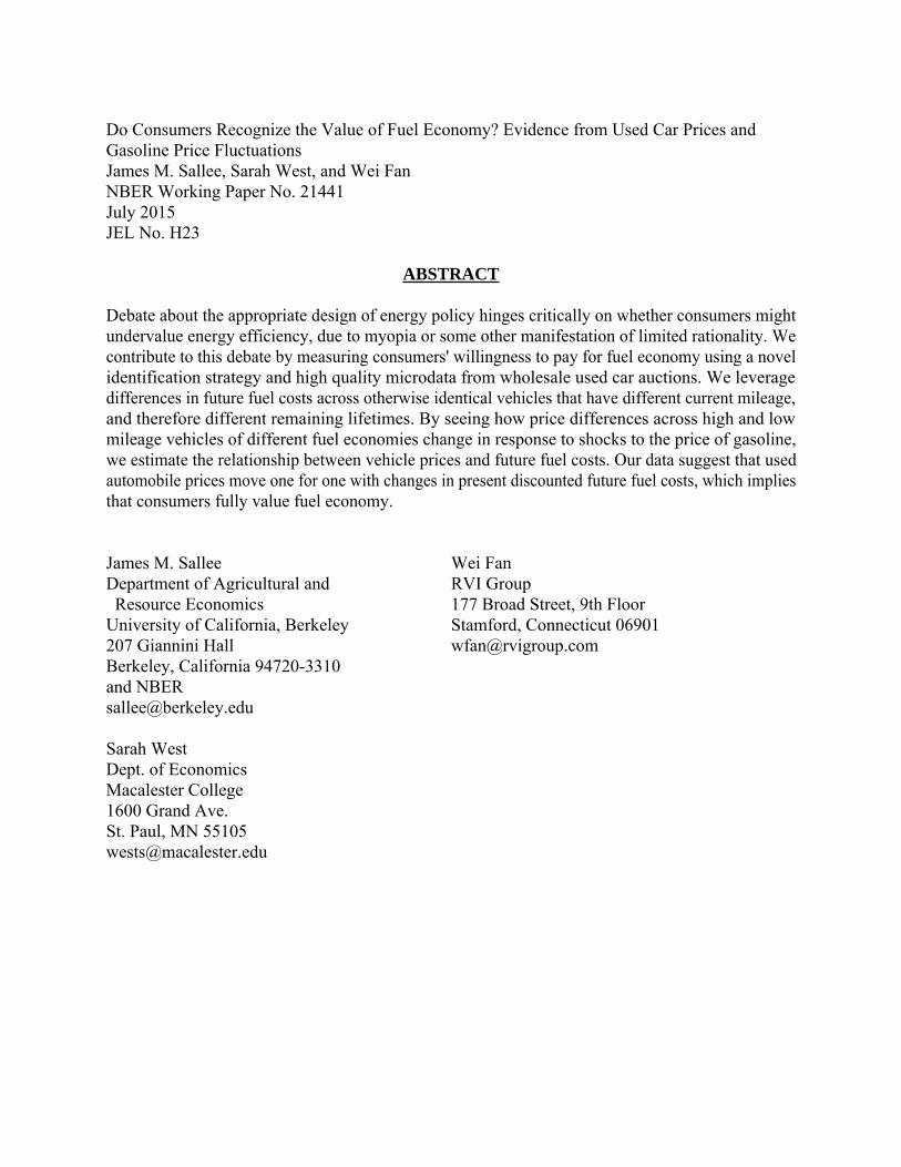
Do Consumers Recognize the Value of Fuel Economy? Evidence from Used Car Prices andGasoline Price FluctuationsJames M. Sallee, Sarah West, and Wei FanNBER Working Paper No. 21441July 2015JEL No. H23

ABSTRACT

Debate about the appropriate design of energy policy hinges critically on whether consumers mightundervalue energy efficiency, due to myopia or some other manifestation of limited rationality. Wecontribute to this debate by measuring consumers' willingness to pay for fuel economy using a novelidentification strategy and high quality microdata from wholesale used car auctions. We leveragedifferences in future fuel costs across otherwise identical vehicles that have different current mileage,and therefore different remaining lifetimes. By seeing how price differences across high and lowmileage vehicles of different fuel economies change in response to shocks to the price of gasoline,we estimate the relationship between vehicle prices and future fuel costs. Our data suggest that usedautomobile prices move one for one with changes in present discounted future fuel costs, which impliesthat consumers fully value fuel economy.

James M. SalleeDepartment of Agricultural and Resource EconomicsUniversity of California, Berkeley207 Giannini HallBerkeley, California 94720-3310and NBERsallee@berkeley.edu

Sarah WestDept. of EconomicsMacalester College1600 Grand Ave.St. Paul, MN 55105wests@macalester.edu

Wei FanRVI Group177 Broad Street, 9th FloorStamford, Connecticut 06901wfan@rvigroup.com

1 Introduction

One of the great questions facing policy makers in the twenty-first century is whether and how

to mitigate greenhouse gas emissions so as to limit climate change. Automobiles are a critical

part of this policy problem—in the U.S., personal transportation accounts for 28% of greenhouse

gas emissions (Environmental Protection Agency 2014). Gasoline consumption maps neatly into

greenhouse gas emissions. This means that a Pigouvian tax on emissions is feasible (in the form

of a gasoline tax). Such a tax can fully restore market efficiency, and alternative policies, such

as fuel economy standards, will have inferior welfare properties, provided that the environmental

externality is the only market failure leading to inefficiencies.1

However, many have argued that another market failure does exist, which is that consumers

undervalue energy efficiency in a variety of choice situations, including automobile markets. The

root of this hypothesis is the observation that engineering estimates of the cost of deploying fuel

saving technologies suggest that privately cost-effective technologies often go unadopted. Jaffe and

Stavins (1994) call this the “energy paradox”. If markets substantially undervalue energy efficiency,

then the dominance of a gasoline tax over regulatory approaches may be broken because alternative

policies may be better able to correct for inefficiencies from mis-valuation.2

Motivated by these policy implications, researchers have sought to use revealed preference data

to determine whether consumers do in fact undervalue fuel economy. In this paper, we add to

this literature by developing a unique identification strategy that utilizes fifteen years worth of

microdata on used vehicle transactions to test whether used vehicle prices change by the amount

predicted by a fully rational asset pricing model. We interpret our results as a test of whether or

not consumers fully value fuel economy, and our results directly provide the parameters necessary

for informed policymaking.

Intuitively, our approach is to first compare the prices of two used cars which are identical

except in their current odometer readings—and therefore in remaining future operating costs—and

second to repeat this comparison when different gasoline prices prevail. We repeat this comparison

1For reviews of the design of policies to correct driving related externalities, see Parry, Walls, and Harrington(2007); Anderson, Parry, Sallee, and Fischer (2011) and Sallee (2011). The efficiency property of a gasoline tax ismore complicated for local pollutants, as is explored in several papers, including Fullerton and West (2002, 2010) andKnittel and Sandler (2012).

2Fischer, Harrington, and Parry (2007), Allcott, Mullainathan, and Taubinsky (2014) and Heutel (2011) explorethe implications of undervaluation for optimal policy design.

1

across many vehicle types and many months, during which changes in the price of gasoline drive

changes in fuel costs, in order to estimate the relationship between vehicle prices and a measure of

the present discounted fuel cost that we construct. For example, we calculate the price and fuel cost

of a 2000 Ford Taurus SE six cylinder 3.0L vehicle with automatic transmission and front-wheel

drive that has 50,000 miles in July 2005 to a different 2000 Ford Taurus SE six cylinder 3.0L vehicle

with automatic transmission and front-wheel drive that has 60,000 miles in July 2005. We then

calculate the price and fuel cost of two different cars with the exact same configuration and mileage

in July 2006. Changes in the gasoline price between July 2005 and July 2006 will cause changes in

the difference in expected fuel costs across the higher and lower mileage vehicles. We test whether

the change in the price difference between the high and low mileage vehicle over time corresponds

to the change in the cost difference.

This is conceptually similar to a difference-in-difference approach. The fact that our comparison

is across vehicles of the same type that differ only in their current mileage allows us to provide

an exceptionally rich set of controls, including time-period shocks and depreciation schedules that

are unique for each vehicle type. Specifically, our preferred specification allows for a unique fixed

effect in every month of our sample for every vehicle type, and it controls for a unique depreciation

schedule for each vehicle type, where a vehicle type is very finely defined. To execute this research

design, we employ used vehicle price data that include actual transaction prices, dates of sale,

vehicle identification numbers, and odometer readings for a large sample of vehicles sold at wholesale

auctions between July 1993 and June 2008.

In our baseline specification, we find that vehicle prices do move one for one with future fuel

costs. This conclusion is robust to a number of specification checks.3 Given some simplifying

assumptions about the structure of the used car market, this result implies that consumers do

value fuel economy properly. This finding casts doubt on the idea that regulatory policies, such as

fuel economy standards, might be more efficient than fuel taxation because they correct both the

environmental externality and private mis-optimization due to limited rationality.

Our data come from wholesale auctions, but our interest is in what consumers pay in the retail

3The main exception is that we find that for our highest mileage cars (those with over 100,000 miles when soldat auction), prices are significantly less responsive to fuel cost shocks. This may indicate that buyers of the oldestand least expensive used cars undervalue fuel economy, but it may also be due to a selection process by which onlycertain types of high mileage vehicles appear in wholesale auctions.

2

market. Using an auxiliary data set from used car guide books, we demonstrate that price changes

in the retail market appear to pass through one to one into retail prices. This is consistent with

a competitive used car market, and it allows us to interpret our wholesale price results as directly

reflecting consumer willingness to pay in the retail used car market.

We are not the first to ask whether or not consumers value fuel economy properly.4 The most

similar existing papers are Allcott and Wozny (2014), Busse, Knittel, and Zettelmeyer (2013) and

Grigolon, Reynaert, and Verboven (2014). These papers use a panel identification strategy that

leverages the fact that common gasoline price shocks translate into different fuel cost shocks for

different vehicles based on their fuel economies.5 Compared to these papers, we are able to relax

a number of restrictive assumptions on the set of control variables. Specifically, because we utilize

differences across vehicles of the same type in the same month by using variation in the odometer,

we can control nonparametrically for time period shocks specific to each vehicle type, and we can

control very flexibly for a depreciation schedule for each vehicle type. These papers find a range of

estimates of consumer valuation across specifications that overlap with each other, where Allcott

and Wozny (2014) emphasize estimates that find modest undervaluation, while Busse, Knittel,

and Zettelmeyer (2013) and Grigolon, Reynaert, and Verboven (2014) emphasize that their results

cannot consistently reject full valuation.

We interpret our estimates as consistent with their results. Moreover, we believe that our

procedure presents a more difficult test because we identify consumer valuation off of variation in

odometers within a set of otherwise identical vehicles, which may not be very salient to consumers.

If consumers have limited attention, in the sense of Sallee (2014), then we might expect them to

ignore the type of within model variation in fuel costs that we leverage. That is, one could imagine

consumers recognizing the fuel cost differences across categories of automobiles, but not “noticing”

the difference in implied fuel costs across high and low mileage versions of the same model.

Our baseline model produces precise estimates consistent with full valuation. Our procedure

yields statistical precision, and our results are robust across a number of dimensions. But, we

emphasize that our procedure can be made to yield different results because it relies on a number

of assumptions about underlying parameters that we use to construct our estimate of the future fuel

4We discuss the literature, and our relationship to it, more fully in the next section.5Linn and Klier (2010) use the same strategy to study sales volumes, rather than prices. Li, Timmins, and von

Haefen (2009) and Jacobsen and van Benthem (Forthcoming) use it to study vehicle scrappage decisions.

3

cost of a vehicle, including consumer discount rates, expectations regarding future gasoline prices,

perceived on road fuel economy, and typical patterns of vehicle utilization and scrappage. We have

empirical support for each of the assumptions we use, but reasonable alternative parameter choices

could shift our coefficient estimate in either direction. The same is true of other papers in the

literature.

Thus, while the literature fails to consistently reject the null hypothesis of full valuation, the

data cannot consistently rule out modest undervaluation, unless one takes a firm stand on underly-

ing parameters that are themselves uncertain. What is clear from our results, in conjunction with

the existing literature, is that the assumption that consumers place a zero value on fuel economy

is indefensible. Nevertheless, this assumption is still employed, implicitly, in regulatory impact

analyses that credit the entire fuel savings of consumers as a benefit of programs like the Cor-

porate Average Fuel Economy (CAFE) standards. If consumers value fuel economy properly and

automakers deploy fuel-saving technologies so long as their cost lies below consumer willingness

to pay, then fuel economy improvements forced upon the market by regulation must be causing a

trade-off in vehicle characteristics or market shares that lowers consumer surplus. This crediting

of fuel savings as a program benefit is often pivotal to the cost-benefit analysis. For example, fuel

savings represent nearly 80% of the total benefits of the 2017-2025 CAFE standards (Environmental

Protection Agency 2012).

Our empirical evidence, combined with the previous literature, implies that consumers at worst

undervalue fuel economy modestly. If there are energy efficient technologies that are not being

deployed, then researchers and regulators should perhaps shift their attention to supply side expla-

nations, like competitive failures, technological spillovers or other hold ups within the automobile

industry.6

The remainder of the paper is structured as follows. Section 2 explains our econometric strategy

in more detail. Section 3 describes our data. Section 4 details the relationship between vehicle price

and odometer in our data. We use this analysis to determine the appropriate set of odometer control

variables. Section 5 reports our main results, along with a variety of robustness checks. Section 6

6Sallee (2014) suggests one possible caveat. He argues that in a model with rational inattention it is possible thatconsumers are attentive to (fully value) the set of energy efficiency technologies that are deployed in equilibrium, butnevertheless there are cost-effective technologies that are not deployed because they are not salient and would beundervalued if they were deployed.

4

concludes.

2 Conceptual approach

Our estimation strategy is based on exploiting variation in the expected future fuel cost of vehicles

resulting from differences in the odometer reading and the price of fuel at the time a vehicle is sold.

For example, suppose that two 2005 Toyota Camrys are sold in November 2009, one with 80,000

miles on the odometer and the other with 90,000 miles. The price difference between these two cars

should reflect the difference in value of having a lower mileage vehicle (which is in better condition

and has a longer expected remaining life) net of the larger operating costs, which are a function of

fuel prices. Next, imagine that the price of gasoline changes between November 2009 and December

2009, and that in December two other 2005 Toyota Camrys, one with 80,000 miles and the other

with 90,000 miles, are sold. Now, the price difference should reflect the same factors as before, and

the difference-in-difference should reflect only the change in operating costs that resulted from the

gasoline price change. There may be many factors that affect the level of these prices, but as long

as these factors have the same effect on an 80,000 mile Camry and a 90,000 mile Camry, they can

be accounted for with fixed effects.

Our final estimating equation has the intuitive flavor of this example, but it is not literally a

difference-in-difference because we use a continuous measure of odometer readings. In the end, we

regress used vehicle transaction prices on a rich set of mileage controls, time period fixed effects and

a measure of the discounted expected future operating costs of vehicles. Our specification allows

different vehicle types to have different depreciation schedules. Specifically, we allow the odometer

polynomial and the time period fixed effects to vary for each vehicle type—where a type is defined

by all observed characteristics contained in the “stub” of the Vehicle Identification Number (VIN),

which includes model name, vintage, cylinders, displacement, and sometimes additional information

on transmission and trim levels. We are able to do this and still identify the parameter because we

use individual transaction prices and use variation in fuel costs within a car type and time period

by exploiting the odometer information.

To arrive at our estimation equation, we start with a simple model of the price of used cars

which assumes that the used car market is competitive, the supply of used cars is inelastic, and

5

that transaction costs are small.7 The logic of the inelastic supply assumption is that, in any given

period, the full stock of used cars (not necessarily the set listed for sale) of a given vintage and

type is fully predetermined. Under these assumptions, the expected discounted price, P , of an

individual vehicle i of type j at time t is equal to the expected discounted value of operating the

car V (·) over its remaining lifetime, minus the expected discounted values of fuel costs C(·), and

maintenance costs Z(·):

Pijt = V (Oijt, Xj , r) − C(Oijt,mijt, gt,MPGj , r) − Z(Oijt, Xj , r), (1)

where O is the car’s mileage (“O” is for odometer) at the start of period j, Xj is a vector of vehicle

attributes, m is per period miles driven, g is the price of gasoline, MPG is the vehicle’s fuel economy

in miles per gallon, and r is the discount rate.

The discounted value of fuel costs, C(·), is given by:

Cijt = E

[T∑s=t

H(Oijt, Xj)

(1

1 + r

)(s−t) mjsgsMPGj

], (2)

where T is the final period at which time all vehicles are scrapped, and H(·) is the probability

of survival of a vehicle as a function of its odometer reading and its attributes. We detail the

construction of this variable in Section 3.1, below.

The fundamental question in the literature on the energy efficiency gap is whether or not con-

sumers fully value fuel economy, which is typically formulated as the existence of a one to one

mapping between price and future discounted fuel costs, in the used car market where supply is

assumed to be perfectly inelastic. Thus, the goal is to find a way to regress prices P on future

discounted fuel costs C that leaves variation in C but protects against omitted variable biases.

Variation in fuel costs comes from several sources. It comes across vehicle types because of differ-

ences in fuel economy. It comes over time because of differences in the price of gasoline. And, it

comes across individual vehicles depending on their remaining lifetime.

Different articles in the literature have used different types of variation, and all approaches

require some assumptions to achieve identification. The cross-sectional hedonic approach that was

7With zero transaction costs, the market allocation will be the same as if people rented a vehicle each period.This abstracts from sorting concerns.

6

once prominent in the literature used variation across vehicle types in studies of new car prices.8

Automobiles have many unobserved characteristics, however, so the cross-sectional approach lacks

credibility as an identification strategy.

The literature recently switched to a focus on the use of panel strategies that use changes

in gasoline prices as a source of quasi-experimental variation (Kahn 1986; Kilian and Sims 2006;

Allcott and Wozny 2014; Busse, Knittel, and Zettelmeyer 2013; Grigolon, Reynaert, and Verboven

2014). A common gasoline price shock creates different fuel cost changes across vehicle types,

because of differences in fuel economy.9 Thus, a single gasoline price time series generates panel

variation that allows for price regressions that include fixed effects for each vehicle type, which will

absorb any time invariant unobserved factors. When the unit of analysis is the same vintage of

vehicle observed several times in the used car market, these fixed effects will capture all attributes

of the vehicle.

This approach uses variation from the interaction of fuel prices and vehicle fuel economy. This

does not require the use of micro data (though it can be used, as in Busse, Knittel, and Zettelmeyer

(2013)) because it uses differences across vehicle types over time, rather than making predictions

about how different vehicles of the same type would differ in price within a time period. As such,

this approach cannot control for vehicle type specific time period shocks; it rests on assumptions

that some broader level of time period fixed effects are able to account for demand shocks that

influence the price of vehicles. If there are demand shocks in different time periods that have

differential effects on different types of vehicles, and if these differential shocks are correlated with

fuel economy, then this approach may still be biased. As suggested in Langer and Miller (2013),

the prices of competing products may be one such source of correlated shocks.

Our approach focuses on vehicle mileage in order to relax those assumptions. We isolate the

effect of fuel price changes over time on the differences in prices across vehicles of the same type in

the same time period, which differ only in their remaining lifetime by virtue of having been driven

more or less prior to that time period.10

8This approach goes back at least to the seminal contributions in Hausman (1979) and Dubin and McFadden (1984)on household durables using cross-sectional data. The cross-sectional literature on automobiles includes Dreyfus andViscusi (1995), Goldberg (1998) and Espey and Nair (2005). This literature found mixed evidence of consumerundervaluation. See Greene (2010) and Helfand and Wolverton (2009) for reviews.

9Grigolon, Reynaert, and Verboven (2014) differ from our approach and from the existing literature on the U.S.in focusing on the demand for diesel versus gasoline vehicles in Europe.

10Our conceptual framework assumes a risk neutral agent who cares only about the average future fuel cost. Risk

7

In addition to requiring micro data, our approach may involve trade-offs, both practical and

conceptual. Practically, our procedure eliminates the vast majority of variation in prices and fuel

costs through our control variables, and the variation that remains may be too small to yield

statistical precision. That turns out not to be the case, both because the gasoline price moves a

great deal during our sample period and because we have a large data set.

Aside from practical concerns, our strategy also has conceptual implications. Like the rest of the

literature that employs panel techniques, our approach identifies the relationship between fuel costs

and prices using variation in fuel costs within a product over time, whereas the ultimate concern

for policy is whether consumers make rational choices between products. It is conceivable that

behavioral agents might make rational choices in one dimension but not the other. This implies

that the move from cross-sectional to panel identification may pose a trade-off—the cross-sectional

literature directly studies the choice situation most of interest to policy, but it is subject to omitted

variable bias.

In our context, we are most concerned that our econometric strategy isolates variation that is

far less salient to consumers than are cross-sectional differences in fuel costs between different types

of automobiles, so that we may have tilted the scales in favor of finding undervaluation. That is,

consumers might ignore differences in fuel costs due to odometer variation, while still accurately

considering the average differences (across all odometer levels) in fuel costs across models.11 If so,

then when gasoline prices rise, consumers would switch demand away from heavy trucks towards

compact cars, but they might simultaneously fail to account for the differential implications of the

gasoline price change for low versus high mileage compact cars. As a result, we think our approach

would be more likely to find undervaluation than the prior literature. The fact that we do not

therefore provides relatively strong evidence in favor of the full valuation null hypothesis.

The opposite could be true—consumers might rationally adjust their evaluation of the lifetime

fuel costs of models with different odometer levels when gasoline prices change, while simultane-

averse agents will perceive some value in more fuel economic vehicles, which condense the variation in fuel costs thatarise from shocks to the future gasoline price. Changes in the volatility of the price of gasoline may therefore influencethe value of fuel economy over our sample period. But, our identification strategy limits this concern. Any increasein demand for a particular car type due to volatility considerations will be soaked up in our vehicle type by timefixed effects.

11Allcott and Wozny (2014) make this same point in discussing our approach versus theirs. Sallee (2014) exploresthe same issue, arguing that, when perfect information is costly to acquire, consumers may be rationally inattentiveto some types of fuel cost variation, while being attentive to others, due to differences in the consequences of ignoringeach type of variation.

8

ously making inconsistent comparisons across models. We are unable to come up with internally

consistent explanations as to why that would happen, but neither can we prove that it is impossible.

Further exploration of this conceptual point would be valuable to the literature.

3 Data

Our used car price data come from a large sample of wholesale used car price auctions. The data

include the transaction price, transaction date, odometer reading and truncated Vehicle Identifi-

cation Number (VIN) of each vehicle sold in several large auction houses. This market does not

include individual end users. Automobile dealers, manufacturers and businesses and governments

that own large fleets sell their vehicles at these auctions. The buyers are licensed used car dealers,

who subsequently resell the vehicles to consumers. Used car dealers routinely use these auctions

to optimize the stock of vehicles they have for sale to final consumers by both buying and selling

vehicles.

Our data sample includes millions of transactions that took place between July 1993 and July

2008.12 We match these vehicles to official EPA fuel economy ratings using all available information

on model, model year, cylinders, displacement, body type, transmission and trim. In the estimation,

we use the combined EPA fuel economy rating. For some early model years and for model years after

2007, we lack a complete VIN decoder and for vehicles made before 1978, there are no fuel economy

ratings. Such vehicles are dropped from our sample. We also drop diesel and hybrid vehicles. In

the results reported here, we focus on a 10% random sample of our data for computational reasons.

We also focus primarily on vehicles sold at auction by dealers, rather than vehicles sold by auto

manufacturers themselves or by fleet operators. We do so because our strategy relies on correctly

specifying the remaining lifetime of vehicles, and we believe that vehicles sold by dealers, which

were owned and operated by consumers, will be more likely to depreciate according to the average

schedule that we use for estimation. That is, vehicles operated by fleet owners and manufacturers

may have been used and maintained differently than those owned by consumers. We do report

results from our preferred specifications on these alternative samples.

12The raw data include some data before 1993, but the coverage is limited. We have access to data through partof 2009, but we limit our sample to the period before the financial crisis.

9

3.1 Estimating Remaining Cost

A critical step in our estimation is the construction of the future fuel cost variable. This construction

requires assumptions, described here, about vehicle mileage and survival rates and about consumers’

beliefs about future gasoline prices and their discount rates. Throughout the paper we interpret

our regressions as tests of whether or not consumers fully value fuel economy, but it is critical to

keep in mind that our tests (and those in the existing literature) depend on the accuracy of these

assumptions, and that modifications of these assumptions will mechanically alter our estimated

coefficients.

Mileage and Scrappage

The cost function (equation 2), specified in discrete form, includes the number of miles to be driven

annually by the vehicle in all future periods. Additionally, since a vehicle might be scrapped,

mileage is multiplied by a survival probability to generate expected miles driven. Finally, future

miles driven are discounted to reflect present values.

We calculate mileage and scrappage using the results reported in Lu (2006), which presents

estimates of average mileage per year and scrappage probabilities for passenger cars and light-

trucks (pick-ups, sport-utility vehicles, and vans) as functions of age in years. To accommodate

our identification strategy, we invert the formulas in Lu (2006) to create future annual mileage

and scrappage probabilities that are a function of current mileage, rather than current age.13 This

enables us to calculate the expected future remaining mileage (and hence fuel cost) of each vehicle,

according to its current odometer reading. We do this separately for cars and trucks.

Describing future mileage and scrappage as a function of current odometer allows us to maintain

econometric identification while controlling more flexibly for price shocks to each VIN stub than

was possible in the prior literature. Specifically, we include VIN stub fixed effects interacted with

13The functional form of the equations in Lu (2006) prevents us from doing the inversion analytically. We thusinvert the equations numerically by using the reported coefficients as a data generating process on simulated data,and then fitting a function to the simulated data via regression. Specifically, for each class of vehicles we generate10,000 observations of a variable, “age,” by multiplying 25 years times a random draw from a uniform distributionranging from zero to one. We then generate another variable, “odometer,” which is the integral of Lu’s estimatedannual miles function over the generated age variable. Then, for each class we regress age on a cubic function ofodometer, the coefficients from which enable us to transform any odometer reading into a predicted age in years,where that predicted age in years is now determined by odometer reading. We use a parallel procedure to invert thescrappage function.

10

dummies for each month of our sample (which is the level of variation of our gasoline price variable).

These fixed effects fully control for the relationship between vehicle age and price, which is desirable

to account for depreciation, but they also fully control for the relationship between age and fuel

cost, so that there is no remaining variation in future fuel cost with which to identify a regression

coefficient. Our insight is that, conditional on age, vehicles with higher odometer readings have less

remaining life, so that there is still variation in fuel costs within a VIN stub crossed with month.

To utilize this variation, we must describe the future mileage and scrappage schedule of a vehicle

as a function of its current odometer, not just its age.

We also use our auction data to introduce heterogeneity in remaining miles driven across makes,

as Lu (2006) does not provide make-specific results (e.g., Dodge). Our procedure simply shifts the

expected future mileage schedule up or down proportionally for different automobile makes. We

first generate a predicted odometer reading for all vehicles in our sample, separately for cars and

trucks, based on age measured in annual increments, using the regression coefficients reported by Lu

(2006). We then regress this predicted odometer reading on the actual odometer reading separately

for each make as follows:

dca = θcmOicm + εicm (3)

where c indexes class, a indexes age, and m indexes make.14 This procedure estimates a unique θcm

for each make, a measure of how much each vehicle make is driven compared to the average across

all makes. We use these θcm to shift the predicted mileage schedules for all vehicles in our sample,

and use the shifted schedules when we assign scrappage probabilities and to adjust the future fuel

costs.

We transform Lu’s scrappage probabilities, which are for new vehicles and therefore not condi-

tional on vehicles having survived to their observed ages, into probabilities that are conditional on

having attained the current odometer reading observed at the time of transaction. This adjustment

requires only that we divide through the mileage schedule by the probability of survival up to the

observed odometer.

14We could also estimate these θ using a data set such as the National Household Travel Survey (NHTS), butwe prefer to use our data to do so, as it contains hundreds of thousands more observations over many years, whichenables us to avoid problems with sparseness over some makes within the NHTS. In addition, specification testingsuggests that introduction of this heterogeneity has virtually no effect on our final estimates, though we maintain itin our baseline to allow some degree of data driven heterogeneity.

11

Finally, having established the future annual mileage and scrappage schedule for each model

conditional on its observed odometer at the time of the transaction, we sum over these annual

valuations to construct the future fuel cost variable. Annual mileage is weighted by conditional

scrappage probabilities and discounted for present value. In constructing the cost measure, we

assume that each vehicle lasts no more than 25 remaining periods from the time of observation.

Since it is weighted by scrappage probabilities and discounted for present value, expected mileage

beyond 25 years in the future is negligible for all vehicles. In all results reported in the paper,

we assume that the vehicle miles traveled and scrappage schedules are independent of the price

of gasoline. There is evidence that the gasoline price affects miles traveled and scrappage, but

these affects are modest. For small changes in the price of gasoline, an envelope theory argument

suggests that any such responses will be second order. In addition, we experimented extensively

with introducing a mileage elasticity and make-specific scrappage elasticities based on results from

Li, Timmins, and von Haefen (2009) and found that our results were insensitive to these additional

considerations.15

Gasoline Price Expectations

The cost function in equation 2 also depends upon the price of gasoline in future periods. We

assume that all consumers use a “no change” forecast—i.e., they expect that the future price of

gasoline in all periods is equal to the current price. This is consistent with evidence on actual

consumer beliefs reported in Anderson, Kellogg, and Sallee (2013). It is also the case that a no

change forecast for oil prices preforms as well, or better than, alternative forecasts based on futures

markets or expert surveys (Alquist and Kilian 2010; Alquist, Kilian, and Vigfusson 2013).

Fuel Economy

Several different fuel economy measures are available. In particular, the EPA reports both ratings

for city and highway driving, along with a combined rating which is a harmonic average of the

15Li, Timmins, and von Haefen (2009) and Jacobsen and van Benthem (Forthcoming) document how scrappagedecisions respond to gasoline prices, and there is a large literature studying the mileage response, including Hughes,Knittel, and Sperling (2008); Gillingham (2011); Knittel and Sandler (2012). Kahn (1986) makes the envelope theoryargument to justify a constant mileage assumption. Kilian and Sims (2006) make the same assumption based on thesame reasoning. Allcott and Wozny (2014) and Busse, Knittel, and Zettelmeyer (2013) assume no mileage responsein their baseline specifications, and, like us, they find that relaxing the assumption has little impact on their results.

12

two. We use the combined rating. In 1986, the EPA adjusted ratings to account for the apparent

discrepancy between the official rating and the actual fuel economy used. Starting in 2008 (which

is the very end of our sample), a significant revision to the test procedures was initiated with the

hopes of improving accuracy further. We use the fuel economy rating published at the time of the

vehicle’s sale, which is the official number still available in the EPA fuel economy guide, without

attempting to adjust for these regime changes.16 Additionally, we assume that the fuel economy

rating is accurate for the life of the vehicle. Some research exists quantifying the degree to which

fuel economy may degrade as a vehicle ages. In principle, it would be possible to adjust for this

in our cost measure, but we suspect that consumers are largely unaware of this phenomenon and

know only a vehicle’s official fuel economy rating.

The Discount Rate

The cost function also includes a discount rate. For our baseline estimates, we use a discount

rate of 5%, which we intend to be a conservative (low) benchmark. Allcott and Wozny (2014)

use 6%, based on the average interest rate on car loans according to the Survey of Consumer

Finance. Alternatives rates could be justified by pointing to borrowing costs or other metrics of

the opportunity cost of funds. We do not believe that it is possible to identify a single correct

discount rate, so we select a low rate and discuss the sensitivity of our results to higher discount

rates.

3.2 Summary Statistics

Before presenting our regression results, we briefly describe the summary statistics for our baseline

sample in Table 1. Our baseline sample includes vehicles sold at auction by automobile dealers

that have mileage between 10,000 and 100,000 miles. (Our reason for making this restriction is

explained in the next section.) The average mileage in this sample is just around 57,500 miles.17

These vehicles are about four and one-half years old on average. Sixty-two percent are cars (as

16Our view is that it is appropriate to use the fuel economy rating most likely available to consumers at the timeof purchase. There is a conversion formula that allows one to estimate how a pre-2008 vintage vehicle’s fuel economyrating would translate into the new regime, but this formula was not available until the last few months of our sample.

17One source of error may exist in the odometer readings for a small fraction of our data. Goh, Fischbeck, andGerard (2007) show that many domestic vehicles built prior to the mid-1990s had five-digit odometers. This leadsto rollover, where it is impossible to tell how many hundreds of thousands of miles a vehicle has been driven. Ourestimates are similar when we look only at vehicles known to have six-digit odometers, such as Toyotas and Hondas.

13

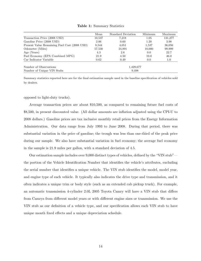
Table 1: Summary Statistics

Mean Standard Deviation Minimum Maximum

Transaction Price (2008 USD) 10,537 7,218 1.05 131,277Gasoline Price (2008 USD) 2.06 0.60 1.20 3.98Present Value Remaining Fuel Cost (2008 USD) 8,544 4,051 1,537 36,056Odometer (Miles) 57,530 24,891 10,000 99,999Age (Years) 4.3 2.6 0.0 22.7Fuel Economy (EPA Combined MPG) 21.9 4.50 10.0 46.0Car Indicator Variable 0.62 0.49 0.0 1.0

Number of Observations 1,429,677Number of Unique VIN Stubs 9,498

Summary statistics reported here are for the final estimation sample used in the baseline specification of vehicles sold

by dealers.

opposed to light-duty trucks).

Average transaction prices are about $10,500, as compared to remaining future fuel costs of

$8,500, in present discounted value. (All dollar amounts are inflation adjusted using the CPI-U to

2008 dollars.) Gasoline prices are tax inclusive monthly retail prices from the Energy Information

Administration. Our data range from July 1993 to June 2008. During that period, there was

substantial variation in the price of gasoline; the trough was less than one-third of the peak price

during our sample. We also have substantial variation in fuel economy; the average fuel economy

in the sample is 21.9 miles per gallon, with a standard deviation of 4.5.

Our estimation sample includes over 9,000 distinct types of vehicles, defined by the “VIN stub”—

the portion of the Vehicle Identification Number that identifies the vehicle’s attributes, excluding

the serial number that identifies a unique vehicle. The VIN stub identifies the model, model year,

and engine type of each vehicle. It typically also indicates the drive type and transmission, and it

often indicates a unique trim or body style (such as an extended cab pickup truck). For example,

an automatic transmission 4-cylinder 2.0L 2005 Toyota Camry will have a VIN stub that differs

from Camrys from different model years or with different engine sizes or transmission. We use the

VIN stub as our definition of a vehicle type, and our specification allows each VIN stub to have

unique month fixed effects and a unique depreciation schedule.

14

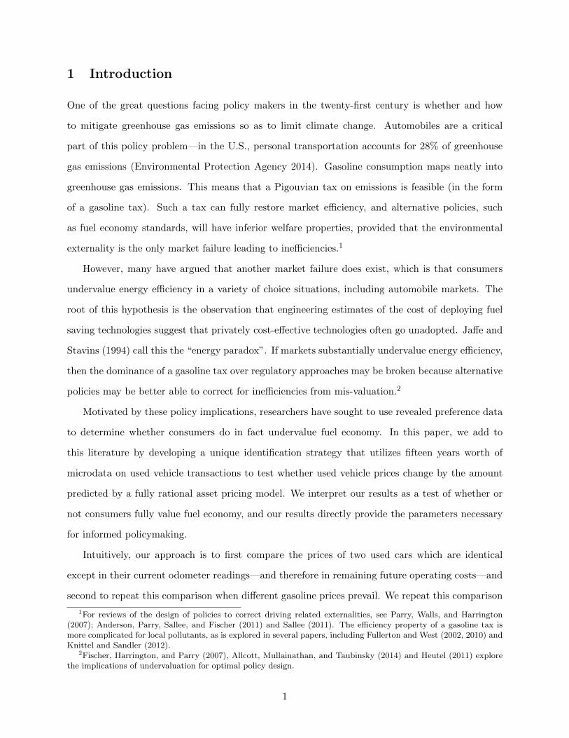
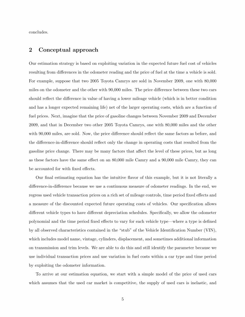
Figure 1: Transaction Prices by Existing Mileage

05,

000

10,0

0015

,000

Aver

age

Pric

e

0 50,000 100,000 150,000 200,000 250,000 300,000 350,000Mileage

Figure plots average transaction prices by 5,000 mile bins.

4 How Do Vehicles Depreciate with Mileage?

Our strategy isolates variation in fuel costs and vehicle price that is driven by variation in the

remaining mileage on a particular vehicle, interacted with changes in the price of gasoline. Because

we are isolating this variation, it is essential to accurately model the relationship between mileage

and vehicle price. Any misspecification of this relationship could bias our results. Thus, before

presenting our main results, we explore the relationship between price and odometer—that is, the

way that vehicles depreciate with use—in our data.

To do so, we take a random sample of one million observations and explore the relationship

between existing mileage at the time the vehicle is sold and its price. We first plot the full sample,

collapsed into 5,000 mile bins, in Figure 1. This shows that there is a strong relationship between

vehicle price and odometer readings, but it also points to several anomalies.

First, at very high mileages, the relationship between mileage and price flattens out, and even

15

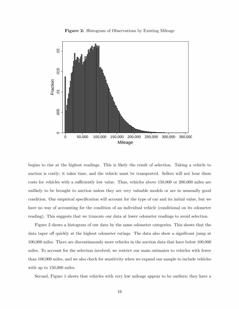
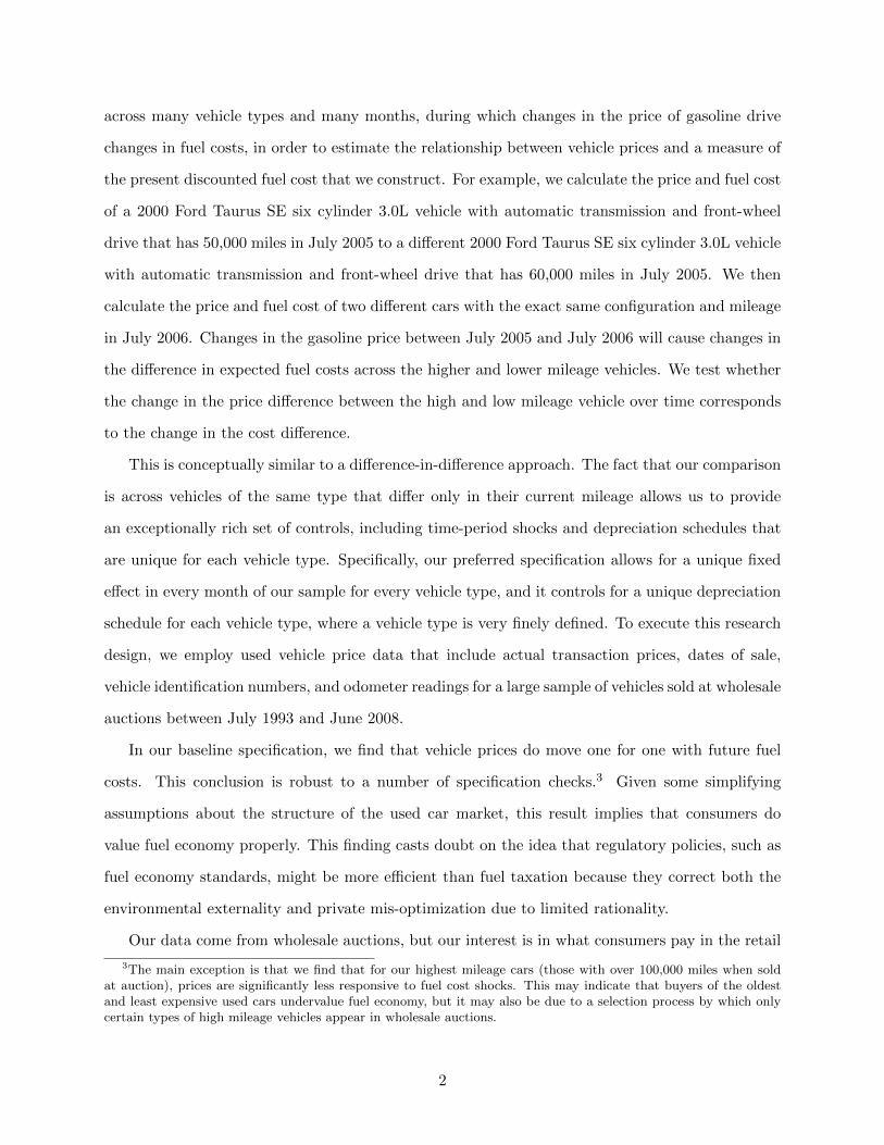
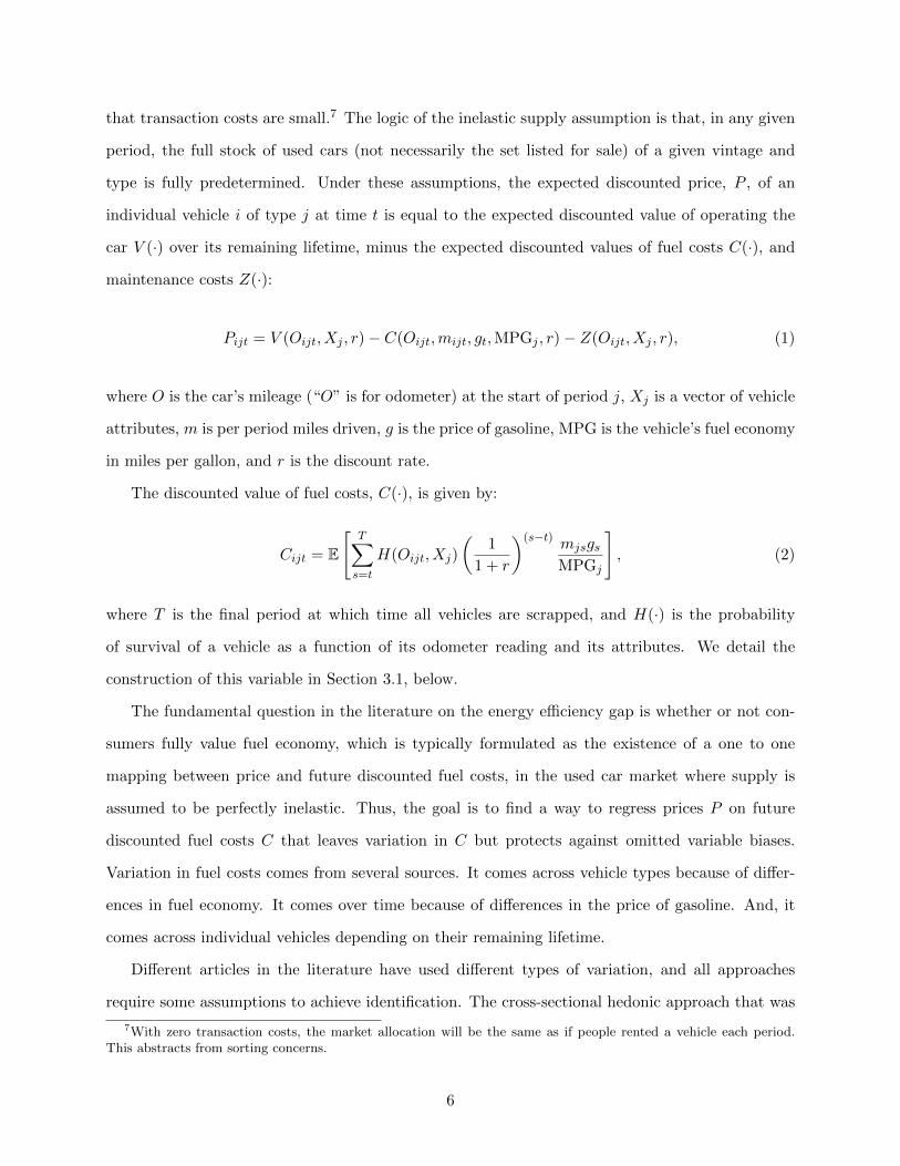
Figure 2: Histogram of Observations by Existing Mileage

0.0

05.0

1.0

15.0

2Fr

actio

n

0 50,000 100,000 150,000 200,000 250,000 300,000 350,000Mileage

begins to rise at the highest readings. This is likely the result of selection. Taking a vehicle to

auction is costly; it takes time, and the vehicle must be transported. Sellers will not bear these

costs for vehicles with a sufficiently low value. Thus, vehicles above 150,000 or 200,000 miles are

unlikely to be brought to auction unless they are very valuable models or are in unusually good

condition. Our empirical specification will account for the type of car and its initial value, but we

have no way of accounting for the condition of an individual vehicle (conditional on its odometer

reading). This suggests that we truncate our data at lower odometer readings to avoid selection.

Figure 2 shows a histogram of our data by the same odometer categories. This shows that the

data taper off quickly at the highest odometer ratings. The data also show a significant jump at

100,000 miles. There are discontinuously more vehicles in the auction data that have below 100,000

miles. To account for the selection involved, we restrict our main estimates to vehicles with fewer

than 100,000 miles, and we also check for sensitivity when we expand our sample to include vehicles

with up to 150,000 miles.

Second, Figure 1 shows that vehicles with very low mileage appear to be outliers; they have a

16

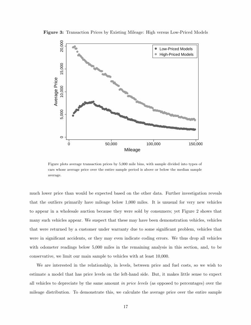
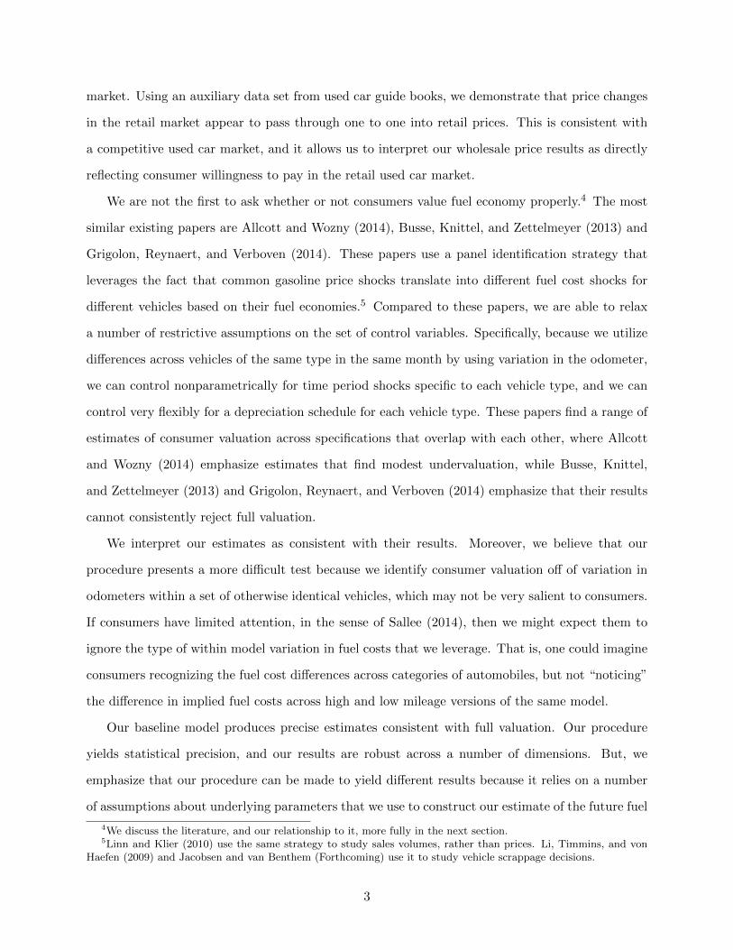
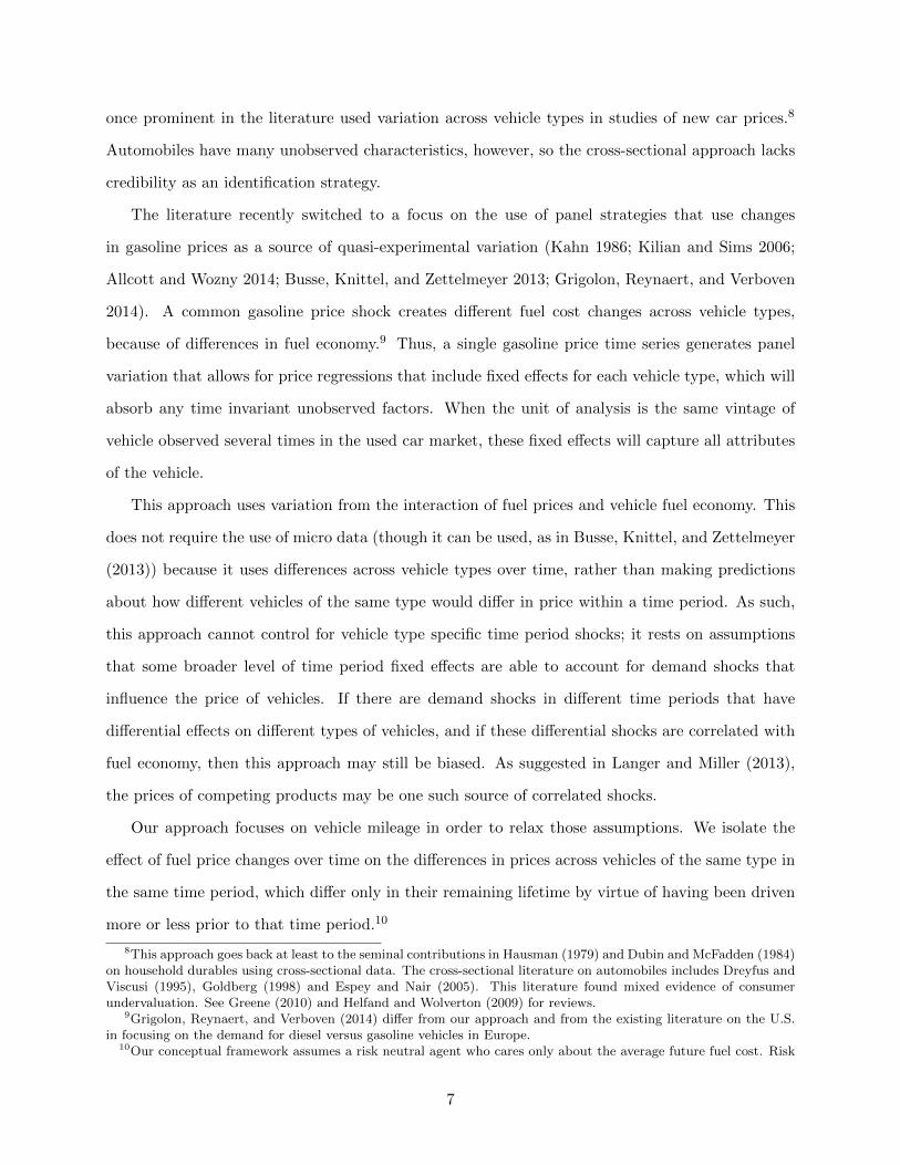
Figure 3: Transaction Prices by Existing Mileage: High versus Low-Priced Models

05,

000

10,0

0015

,000

20,0

00Av

erag

e Pr

ice

0 50,000 100,000 150,000Mileage

Low-Priced ModelsHigh-Priced Models

Figure plots average transaction prices by 5,000 mile bins, with sample divided into types of

cars whose average price over the entire sample period is above or below the median sample

average.

much lower price than would be expected based on the other data. Further investigation reveals

that the outliers primarily have mileage below 1,000 miles. It is unusual for very new vehicles

to appear in a wholesale auction because they were sold by consumers; yet Figure 2 shows that

many such vehicles appear. We suspect that these may have been demonstration vehicles, vehicles

that were returned by a customer under warranty due to some significant problem, vehicles that

were in significant accidents, or they may even indicate coding errors. We thus drop all vehicles

with odometer readings below 5,000 miles in the remaining analysis in this section, and, to be

conservative, we limit our main sample to vehicles with at least 10,000.

We are interested in the relationship, in levels, between price and fuel costs, so we wish to

estimate a model that has price levels on the left-hand side. But, it makes little sense to expect

all vehicles to depreciate by the same amount in price levels (as opposed to percentages) over the

mileage distribution. To demonstrate this, we calculate the average price over the entire sample

17

period for each type of vehicle and, according to this average, define vehicle types as either above or

below average in price. Figure 3 plots the high and low priced vehicles separately to demonstrate

that, in level terms, high priced vehicles depreciate faster. In general, different vehicles can be

expected to depreciate according to a different schedule, and this is particularly true when measured

in level dollars. Moreover, fuel economy is correlated with price (in our raw data this correlation is

negative), which heightens concerns about bias if the depreciation schedule is not specified correctly

for each model. To account for this, we allow each type of vehicle (VIN stub) in our sample to

depreciate according to a unique schedule. This differs substantially from existing literature, and

it represents one of the key benefits of our microdata approach.18

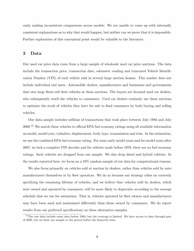
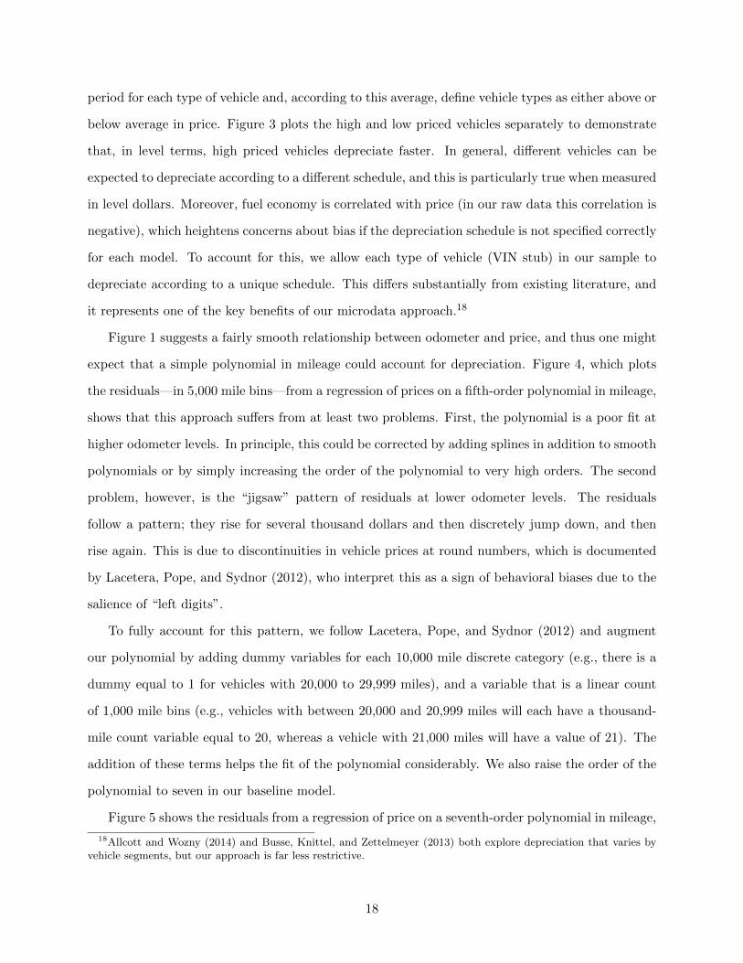
Figure 1 suggests a fairly smooth relationship between odometer and price, and thus one might

expect that a simple polynomial in mileage could account for depreciation. Figure 4, which plots

the residuals—in 5,000 mile bins—from a regression of prices on a fifth-order polynomial in mileage,

shows that this approach suffers from at least two problems. First, the polynomial is a poor fit at

higher odometer levels. In principle, this could be corrected by adding splines in addition to smooth

polynomials or by simply increasing the order of the polynomial to very high orders. The second

problem, however, is the “jigsaw” pattern of residuals at lower odometer levels. The residuals

follow a pattern; they rise for several thousand dollars and then discretely jump down, and then

rise again. This is due to discontinuities in vehicle prices at round numbers, which is documented

by Lacetera, Pope, and Sydnor (2012), who interpret this as a sign of behavioral biases due to the

salience of “left digits”.

To fully account for this pattern, we follow Lacetera, Pope, and Sydnor (2012) and augment

our polynomial by adding dummy variables for each 10,000 mile discrete category (e.g., there is a

dummy equal to 1 for vehicles with 20,000 to 29,999 miles), and a variable that is a linear count

of 1,000 mile bins (e.g., vehicles with between 20,000 and 20,999 miles will each have a thousand-

mile count variable equal to 20, whereas a vehicle with 21,000 miles will have a value of 21). The

addition of these terms helps the fit of the polynomial considerably. We also raise the order of the

polynomial to seven in our baseline model.

Figure 5 shows the residuals from a regression of price on a seventh-order polynomial in mileage,

18Allcott and Wozny (2014) and Busse, Knittel, and Zettelmeyer (2013) both explore depreciation that varies byvehicle segments, but our approach is far less restrictive.

18

Figure 4: Transaction Price Residuals by Existing Mileage from Fifth-Order Polynomial

-400

-200

020

040

0Pr

ice

Res

idua

l

0 50,000 100,000 150,000Mileage

Figure plots average price residuals by 5,000 mile bins from a regression of prices on a fifth-

order polynomial, omitting vehicles with fewer than 5,000 miles or more than 150,000 miles.

19

Figure 5: Transaction Price Residuals by Existing Mileage from Seventh-Order Polynomial withCategorical Controls

-200

-100

010

020

0Pr

ice

Res

idua

l

0 50,000 100,000 150,000Mileage

Figure plots average price residuals by 5,000 mile bins from a regression of prices on a seventh-

order polynomial, a set of dummy variables for each 10,000 odometer category and a linear

control for discrete 1,000 mile categories. The sample omits vehicles with fewer than 5,000

miles or more than 150,000 miles.

20

with dummies for each 10,000 mile category, and the linear one thousand mile discrete category

variable. This specification eliminates the patterns in the residuals. We use this specification as

our baseline. Figure 5 estimates a single (level) depreciation curve for all models, which hides the

variation across types that is highlighted above in Figure 3. Our preferred estimator allows each

model to depreciate in a unique pattern.

It is important to note that this set of odometer control variables accounts for the vast majority

of the overall variation in vehicle prices and future fuel costs. We suspect that the remaining

variation, which comes from differences in remaining lifetime within vehicles of the same type sold

in the same month, is less salient to consumers and thus our specification presents a harsher test

of the full valuation hypothesis than the approach taken in the related literature.

5 Results

Having arrived at a preferred specification through the examination of the relationship between price

and odometer, we use our data to estimate the relationship between prices and present discounted

value future fuel costs in the following estimating equation:

Pijt = βCijt + δjt +J∑

j=1

(7∑

a=1

αjaOaijt +

10∑k=1

γjkdkijt + ρjlijt

)+ εijt (4)

where dkijt =

1 if (k − 1) × 10, 000 < Oijt < k × 10, 000

0 otherwise

lijt = integer floor(Oijt/1000).

In equation 4, Pijt is the real transaction price of vehicle i of VIN stub type j sold in month t,

and Cijt is the remaining future fuel cost for that vehicle. The additional controls include δjt,

which is a vector of VIN stub by month of sample fixed effects (e.g., a fixed effect for an automatic

4-cylinder 2.0L 2005 Toyota Camry in January 2008), and a function of the vehicle’s odometer

reading, denoted Oijt.

The odometer function includes a polynomial, denoted by the Oaijt terms, where a is an exponent

ranging, in our baseline model, from one to seven. It also includes a set of dummy variables for

21

each 10,000 odometer bin, denoted as γjk, and a linear control for the discrete thousand mile bin,

denoted lijt, for each vehicle. As described above, these discrete odometer controls are used to

account for the discontinuous relationship between price and mileage that is analyzed by Lacetera,

Pope, and Sydnor (2012). Importantly, the odometer control function is estimated separately for

each vehicle type j, which is indicated by the outside summation term. This allows each type of

vehicle to depreciate in a unique way, which we believe is essential in a regression on price levels

and in a sample with a diverse set of vehicles.

Our object of interest is β. If consumers fully value changes in fuel economy, we would expect

β to be equal to negative one. That is, a one dollar increase in the present discounted value of

the cost of operating a vehicle over its remaining life should correspond to a one dollar drop in

consumer willingness to pay for the vehicle, which, under the assumptions about market structure

that are outlined in our conceptual model (section 2), will translate into a one dollar drop in price.

Along with β, the δ, α, γ and ρ terms are all parameters to be estimated.

Explaining how we actually estimate this equation may be useful for explaining its full flexibility.

The equation includes many thousands of parameters. To estimate the model we make use of the

Frisch-Waugh-Lovell theorem and first regress prices Pijt, and then costs Cijt, on time period fixed

effects and the odometer control variables for each vehicle type j separately, one at a time. We

then regress the residuals from these two sets of regressions on each other to recover β̂, which

returns numerically identical coefficients to the full model estimated in a single step. (We collect

the number of parameters estimated and use them to make the proper degrees of freedom correction

when calculating standard errors in the second step.) We exclude VIN stubs for which we have

insufficient observations to estimate the first-step regression.

Table 2 reports our main results. Our baseline estimate yields a coefficient estimate of -1.01, with

a standard error of 0.04.19 This estimate is statistically indistinguishable from -1, which represents

the full valuation null hypothesis. It is precise enough to rule out significant undervaluation or

overvaluation. Our estimate changes little when we study only cars or only light-trucks (columns

2 and 3).20 Decreasing the order of the control polynomial to five, or increasing it to nine, has

19All standard errors are clustered at the VIN stub level.20Our baseline model incorporates heterogeneity in the mileage schedules by automobile make, as described above.

Results are very similar when we omit this step and use the unadjusted national average for all vehicles. For example,unadjusted results corresponding to columns 1 to 3 in Table 2 are -1.02, -0.99 and -1.05 respectively.

22

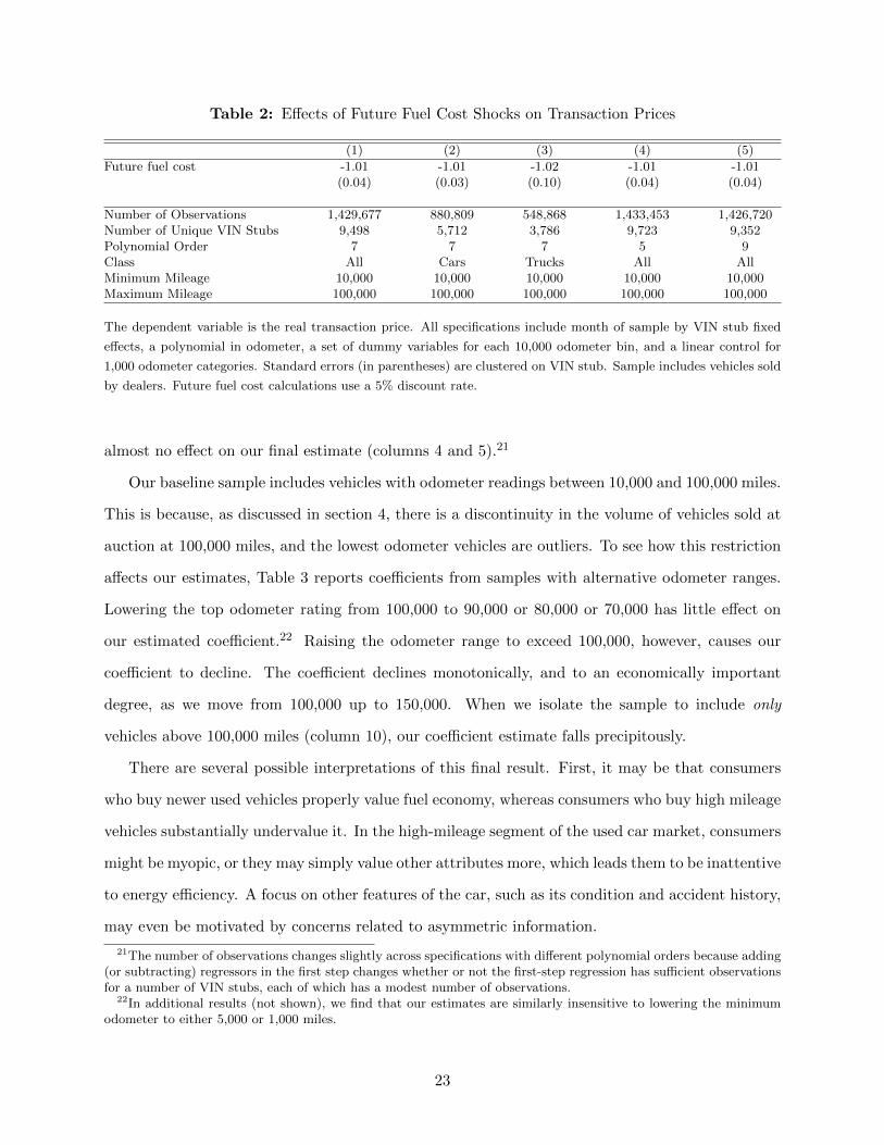
Table 2: Effects of Future Fuel Cost Shocks on Transaction Prices

(1) (2) (3) (4) (5)

Future fuel cost -1.01 -1.01 -1.02 -1.01 -1.01(0.04) (0.03) (0.10) (0.04) (0.04)

Number of Observations 1,429,677 880,809 548,868 1,433,453 1,426,720Number of Unique VIN Stubs 9,498 5,712 3,786 9,723 9,352Polynomial Order 7 7 7 5 9Class All Cars Trucks All AllMinimum Mileage 10,000 10,000 10,000 10,000 10,000Maximum Mileage 100,000 100,000 100,000 100,000 100,000

The dependent variable is the real transaction price. All specifications include month of sample by VIN stub fixed

effects, a polynomial in odometer, a set of dummy variables for each 10,000 odometer bin, and a linear control for

1,000 odometer categories. Standard errors (in parentheses) are clustered on VIN stub. Sample includes vehicles sold

by dealers. Future fuel cost calculations use a 5% discount rate.

almost no effect on our final estimate (columns 4 and 5).21

Our baseline sample includes vehicles with odometer readings between 10,000 and 100,000 miles.

This is because, as discussed in section 4, there is a discontinuity in the volume of vehicles sold at

auction at 100,000 miles, and the lowest odometer vehicles are outliers. To see how this restriction

affects our estimates, Table 3 reports coefficients from samples with alternative odometer ranges.

Lowering the top odometer rating from 100,000 to 90,000 or 80,000 or 70,000 has little effect on

our estimated coefficient.22 Raising the odometer range to exceed 100,000, however, causes our

coefficient to decline. The coefficient declines monotonically, and to an economically important

degree, as we move from 100,000 up to 150,000. When we isolate the sample to include only

vehicles above 100,000 miles (column 10), our coefficient estimate falls precipitously.

There are several possible interpretations of this final result. First, it may be that consumers

who buy newer used vehicles properly value fuel economy, whereas consumers who buy high mileage

vehicles substantially undervalue it. In the high-mileage segment of the used car market, consumers

might be myopic, or they may simply value other attributes more, which leads them to be inattentive

to energy efficiency. A focus on other features of the car, such as its condition and accident history,

may even be motivated by concerns related to asymmetric information.

21The number of observations changes slightly across specifications with different polynomial orders because adding(or subtracting) regressors in the first step changes whether or not the first-step regression has sufficient observationsfor a number of VIN stubs, each of which has a modest number of observations.

22In additional results (not shown), we find that our estimates are similarly insensitive to lowering the minimumodometer to either 5,000 or 1,000 miles.

23

Table 3: Effects of Future Fuel Cost Shocks on Transaction Prices

(1) (2) (3) (4) (5)

Future fuel cost -0.96 -1.04 -1.04 -1.01 -0.98(0.07) (0.06) (0.05) (0.04) (0.03)

Number of Observations 820,297 1,014,319 1,217,404 1,429,677 1,589,980Number of Unique VIN Stubs 7,619 8,319 8,907 9,498 9,802Polynomial Order 7 7 7 7 7Minimum Mileage 10,000 10,000 10,000 10,000 10,000Maximum Mileage 70,000 80,000 90,000 100,000 110,000

(6) (7) (8) (9) (10)

Future fuel cost -0.91 -0.84 -0.78 -0.74 -0.30(0.02) (0.02) (0.01) (0.01) (0.02)

No. of Observations 1,733,144 1,851,912 1,947,666 2,021,138 382,541No. of Unique VIN Stubs 10,077 10,246 10,384 10,476 4,427Polynomial Order 7 7 7 7 7Minimum Mileage 10,000 10,000 10,000 10,000 100,000Maximum Mileage 120,000 130,000 140,000 150,000 150,000

The dependent variable is the real transaction price. All specifications include month of sample by VIN stub fixed

effects, a polynomial in odometer, a set of dummy variables for each 10,000 odometer bin, and a linear control for

1,000 odometer categories. Standard errors (in parentheses) are clustered on VIN stub. Sample includes vehicles sold

by dealers.

Second, consumers who purchase older, lower priced vehicles may, on average, have substantially

higher discount rates. Assuming that they are lower income on average, they are more likely to face

liquidity constraints and will be forced to borrow at higher interest rates, which will (rationally)

drive up the rate at which they trade off future discounted fuel costs against price.

Third, the result could be driven by selection. As argued above, the set of very high mileage

vehicles that appear at wholesale auctions are a selected group. Among this selected group, our

assumption about remaining lifetime mileage, which is based on the national averages reported in

Lu (2006), may be biased. Critically, it could be that consumers who buy older vehicles do so

because they intend to drive very few miles. Thus, we choose to emphasize our baseline sample,

but the results for the high odometer vehicles is a notable caveat to our main results.

Our results align well with the existing literature. Allcott and Wozny (2014) find significant

undervaluation among the oldest models in their sample, but full (or nearly full) valuation among

the newest models.23 Busse, Knittel, and Zettelmeyer (2013), who intepret their findings as consis-

23When Allcott and Wozny (2014) use mileage and scrappage schedules from Lu (2006), as we do, they get anestimate of -1.03 for the newest models (1 to 3 years old) and -0.28 for the oldest models (11 to 15 years old) in theirsample (see their Table 5, column 2). This matches closely to our estimates of -1.01 for the baseline and -0.30 for the

24

tent with full valuation, do not report estimates separately by the age of vehicles in their sample,

but their sample is drawn from vehicles sold at used car dealerships that also have a new car retail

business. This leads their sample to be relatively low odometer (and high priced). Their sample

is thus more similar to ours when we restrict to lower odometer vehicles. (Even then, our vehicles

are somewhat older and less expensive on average.)

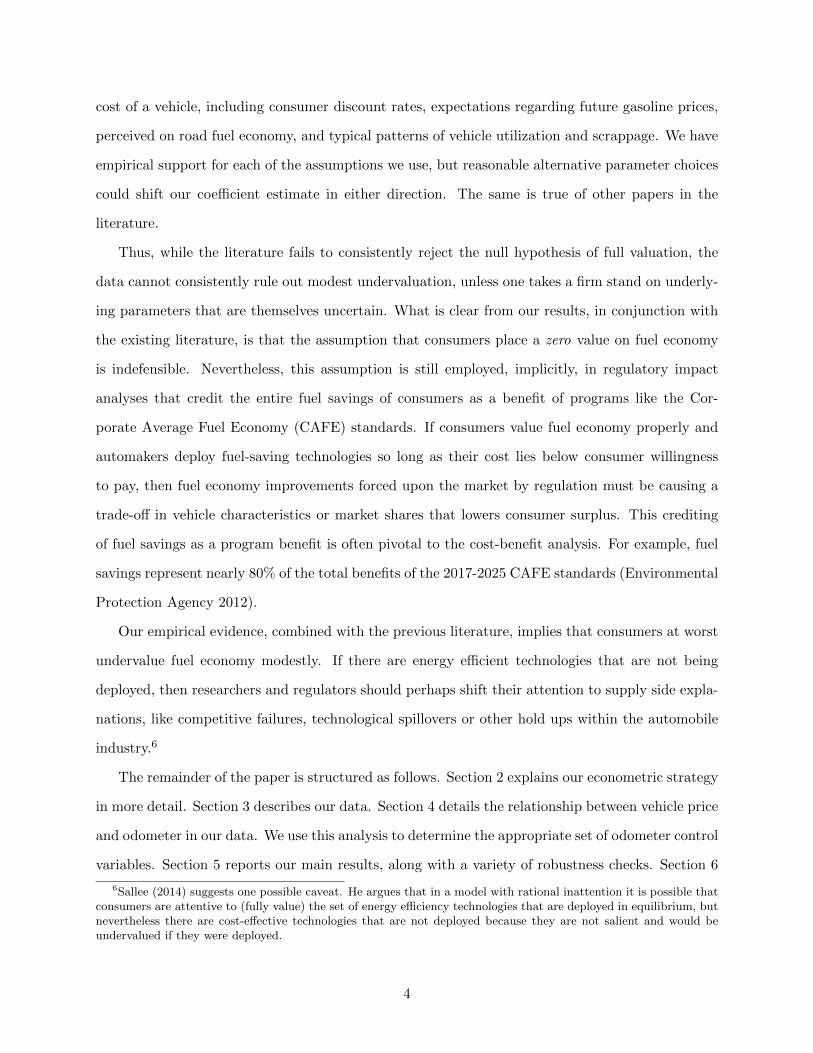
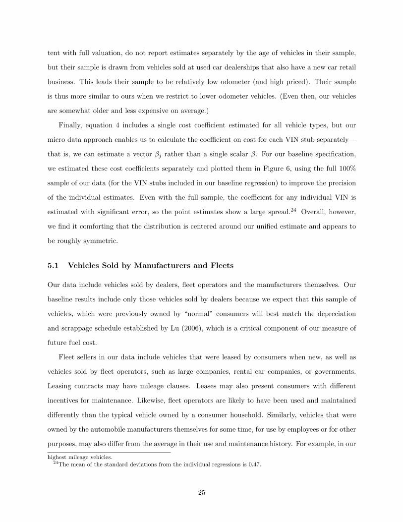
Finally, equation 4 includes a single cost coefficient estimated for all vehicle types, but our

micro data approach enables us to calculate the coefficient on cost for each VIN stub separately—

that is, we can estimate a vector βj rather than a single scalar β. For our baseline specification,

we estimated these cost coefficients separately and plotted them in Figure 6, using the full 100%

sample of our data (for the VIN stubs included in our baseline regression) to improve the precision

of the individual estimates. Even with the full sample, the coefficient for any individual VIN is

estimated with significant error, so the point estimates show a large spread.24 Overall, however,

we find it comforting that the distribution is centered around our unified estimate and appears to

be roughly symmetric.

5.1 Vehicles Sold by Manufacturers and Fleets

Our data include vehicles sold by dealers, fleet operators and the manufacturers themselves. Our

baseline results include only those vehicles sold by dealers because we expect that this sample of

vehicles, which were previously owned by “normal” consumers will best match the depreciation

and scrappage schedule established by Lu (2006), which is a critical component of our measure of

future fuel cost.

Fleet sellers in our data include vehicles that were leased by consumers when new, as well as

vehicles sold by fleet operators, such as large companies, rental car companies, or governments.

Leasing contracts may have mileage clauses. Leases may also present consumers with different

incentives for maintenance. Likewise, fleet operators are likely to have been used and maintained

differently than the typical vehicle owned by a consumer household. Similarly, vehicles that were

owned by the automobile manufacturers themselves for some time, for use by employees or for other

purposes, may also differ from the average in their use and maintenance history. For example, in our

highest mileage vehicles.24The mean of the standard deviations from the individual regressions is 0.47.

25

Figure 6: Histogram of Valuation Coefficient for Individual VIN Stubs

0.0

2.0

4.0

6.0

8Fr

actio

n

-5 -4 -3 -2 -1 0 1 2 3 4Cost Coefficient

Each data point is the cost coefficient from equation 4 estimated for a single VIN stub. The

vertical line is the point estimate from the joint regression from the same specification, which

is found in Table 2, column 1.

sample, both fleet and manufacturer sold vehicles have much higher annual mileage than vehicles

sold by dealers.25 As a result, these vehicles may have expected remaining lifetimes, conditional on

current mileage, that differ from the national average.

Nevertheless, we present our baseline specification for vehicles sold by fleet operators and manu-

facturers in Table 4 for comparison. Column 1 repeats our main estimate from Table 2 for reference,

and columns 3 and 5 show the corresponding result for fleet and manufacturer sold vehicles, re-

spectively. Estimates from these samples suggest modest undervaluation, assuming a 5% discount

rate. The point estimate for fleet operators is -0.86, while that for vehicles sold by manufacturers

is -0.70. This could imply that these automobiles have indeed been depreciated differently than

vehicles sold by dealers at auction.

The even numbered columns in Table 4 show what happens if we recalculate our estimates

25A full set of summary statistics for fleet and manufacturer sold vehicles are included in the appendix.

26

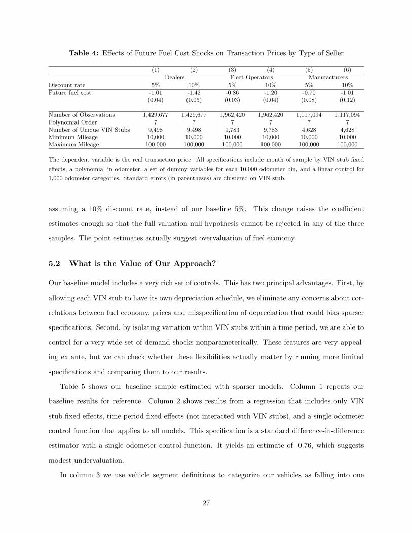
Table 4: Effects of Future Fuel Cost Shocks on Transaction Prices by Type of Seller

(1) (2) (3) (4) (5) (6)

Dealers Fleet Operators ManufacturersDiscount rate 5% 10% 5% 10% 5% 10%

Future fuel cost -1.01 -1.42 -0.86 -1.20 -0.70 -1.01(0.04) (0.05) (0.03) (0.04) (0.08) (0.12)

Number of Observations 1,429,677 1,429,677 1,962,420 1,962,420 1,117,094 1,117,094Polynomial Order 7 7 7 7 7 7Number of Unique VIN Stubs 9,498 9,498 9,783 9,783 4,628 4,628Minimum Mileage 10,000 10,000 10,000 10,000 10,000 10,000Maximum Mileage 100,000 100,000 100,000 100,000 100,000 100,000

The dependent variable is the real transaction price. All specifications include month of sample by VIN stub fixed

effects, a polynomial in odometer, a set of dummy variables for each 10,000 odometer bin, and a linear control for

1,000 odometer categories. Standard errors (in parentheses) are clustered on VIN stub.

assuming a 10% discount rate, instead of our baseline 5%. This change raises the coefficient

estimates enough so that the full valuation null hypothesis cannot be rejected in any of the three

samples. The point estimates actually suggest overvaluation of fuel economy.

5.2 What is the Value of Our Approach?

Our baseline model includes a very rich set of controls. This has two principal advantages. First, by

allowing each VIN stub to have its own depreciation schedule, we eliminate any concerns about cor-

relations between fuel economy, prices and misspecification of depreciation that could bias sparser

specifications. Second, by isolating variation within VIN stubs within a time period, we are able to

control for a very wide set of demand shocks nonparameterically. These features are very appeal-

ing ex ante, but we can check whether these flexibilities actually matter by running more limited

specifications and comparing them to our results.

Table 5 shows our baseline sample estimated with sparser models. Column 1 repeats our

baseline results for reference. Column 2 shows results from a regression that includes only VIN

stub fixed effects, time period fixed effects (not interacted with VIN stubs), and a single odometer

control function that applies to all models. This specification is a standard difference-in-difference

estimator with a single odometer control function. It yields an estimate of -0.76, which suggests

modest undervaluation.

In column 3 we use vehicle segment definitions to categorize our vehicles as falling into one

27

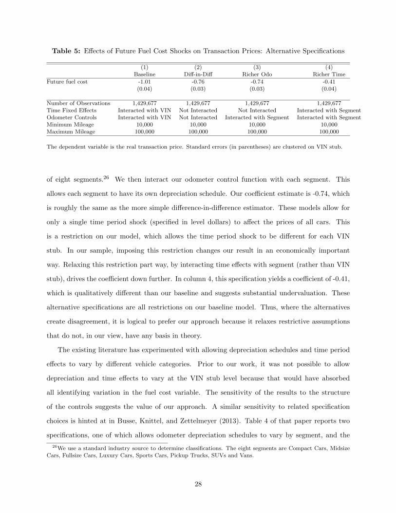
Table 5: Effects of Future Fuel Cost Shocks on Transaction Prices: Alternative Specifications

(1) (2) (3) (4)Baseline Diff-in-Diff Richer Odo Richer Time

Future fuel cost -1.01 -0.76 -0.74 -0.41(0.04) (0.03) (0.03) (0.04)

Number of Observations 1,429,677 1,429,677 1,429,677 1,429,677Time Fixed Effects Interacted with VIN Not Interacted Not Interacted Interacted with SegmentOdometer Controls Interacted with VIN Not Interacted Interacted with Segment Interacted with SegmentMinimum Mileage 10,000 10,000 10,000 10,000Maximum Mileage 100,000 100,000 100,000 100,000

The dependent variable is the real transaction price. Standard errors (in parentheses) are clustered on VIN stub.

of eight segments.26 We then interact our odometer control function with each segment. This

allows each segment to have its own depreciation schedule. Our coefficient estimate is -0.74, which

is roughly the same as the more simple difference-in-difference estimator. These models allow for

only a single time period shock (specified in level dollars) to affect the prices of all cars. This

is a restriction on our model, which allows the time period shock to be different for each VIN

stub. In our sample, imposing this restriction changes our result in an economically important

way. Relaxing this restriction part way, by interacting time effects with segment (rather than VIN

stub), drives the coefficient down further. In column 4, this specification yields a coefficient of -0.41,

which is qualitatively different than our baseline and suggests substantial undervaluation. These

alternative specifications are all restrictions on our baseline model. Thus, where the alternatives

create disagreement, it is logical to prefer our approach because it relaxes restrictive assumptions

that do not, in our view, have any basis in theory.

The existing literature has experimented with allowing depreciation schedules and time period

effects to vary by different vehicle categories. Prior to our work, it was not possible to allow

depreciation and time effects to vary at the VIN stub level because that would have absorbed

all identifying variation in the fuel cost variable. The sensitivity of the results to the structure

of the controls suggests the value of our approach. A similar sensitivity to related specification

choices is hinted at in Busse, Knittel, and Zettelmeyer (2013). Table 4 of that paper reports two

specifications, one of which allows odometer depreciation schedules to vary by segment, and the

26We use a standard industry source to determine classifications. The eight segments are Compact Cars, MidsizeCars, Fullsize Cars, Luxury Cars, Sports Cars, Pickup Trucks, SUVs and Vans.

28

other allows it to vary by fuel economy quartile. The choice has a significant impact on their

results, and the authors make an argument about which set of controls is preferred a priori. A

principle benefit of our specification is that we need not make such choices, but rather can use a

more general set of controls.

5.3 How Do Wholesale Price Changes Influence Retail Prices?

Our interest is in how consumer prices change in response to future fuel cost changes, but our

data are from wholesale auctions. Dealers purchase vehicles at these auctions and pass them on to

consumers. To the extent that the used car market is competitive, we would expect wholesale price

shocks to be passed on one for one into retail consumer prices. If so, then our regression coefficients

can be directly interpreted as the effect of fuel cost shocks on consumer prices. Alternatively, if

used car dealers add a proportional markup over the purchase price, then our coefficient estimates

should be “scaled up”. We find support for a one to one relationship between wholesale and retail

prices using an auxiliary data set.

To examine the relationship between wholesale and retail prices, we use data from Kelley Blue

Book. To measure wholesale prices, Kelley Blue Book collects data from auctions. To measure

retail prices, they gather data on actual transactions from dealers and other market data sources.

We gathered the wholesale and retail prices of all available cars and light-trucks in the July edition

of the Kelley Blue Book guide from 2003 to 2008. We then regress a vehicle’s retail price on its

wholesale price to determine price pass through.

Table 6 reports our results. The first column presents simple OLS results. The unit of observa-

tion is a particular model and vintage sold in July of each year. We include year dummy variables

and age dummy variables in all specifications. In the OLS specification, most of the variation

in prices comes from differences across models. The OLS coefficient implies that when wholesale

prices rise by $1, retail prices rise by $1.03. This is not statistically different from the one to one

benchmark.27

We change the source of identification by adding model by vintage fixed effects in column 2. In

this specification, pass through is identified only from changes in the price of particular models over

27This does not imply that retail and wholesale prices are the same. Rather, our data show that average markupsof retail prices over wholesale prices are quite high, on the order of 30%. But, this may reflect fixed costs of shipping,repairing, holding and selling vehicles that do not vary with the wholesale price of the vehicle.

29

Table 6: Pass Through of Wholesale Price Changes to Retail Prices

OLS FE IV(1) (2) (3)

Wholesale Price 1.03 0.64 1.05(0.06) (0.21) (0.05)

Number of Observations 29,318 29,318 29,318Year Dummies Yes Yes YesAge Dummies Yes Yes YesVIN Stub Dummies No Yes Yes

First-stage F-statistic 428

Dependent variable is the retail price of a vehicle, as reported by Kelley Blue Book. In column 3, the instrument is

the interaction between each vehicle’s fuel economy rating and the current real price of gasoline.

time, controlling for year and age effects. These fixed effects soak up a majority of the variation,

which is reflected in a much higher standard error. The coefficient falls significantly, though it is

still not statistically different from 1. The reduction in the coefficient may reflect attenuation from

measurement error, which is exacerbated by the panel strategy.

Both to overcome possible measurement error attenuation in the panel and to provide a more

solid identification strategy, we use an instrumental variables approach in the third column. We

instrument wholesale prices using the interaction of fuel economy and the price of gasoline in that

year. This instrument isolates variation in wholesale prices due to price shocks associated with

gasoline price changes. This is a valid instrument if the only way that fuel economy interacted

with gasoline prices affects retail prices is “through wholesale prices”, which is consistent with

interpreting wholesale prices as the outside option for a dealer who is deciding whether to hold and

sell a particular model or to take it to auction and swap it for another model to have on their lot.

Our instrument is very powerful in the first stage.

The IV estimates are quite similar to the OLS. The point estimate implies a very small pro-

portional markup, at 5%, of retail over wholesale prices. Taken at face value, this implies that

our estimates from the auction data could be scaled up by 5%, which would change none of our

qualitative conclusions. The standard error is not tight enough to rule out perfect pass through,

however, and so we prefer to interpret these results as a failure to reject a null hypothesis of one to

one pass through. This is consistent with the used car market being competitive. Under that inter-

pretation, our main results can be interpreted directly as estimates of consumer valuation without

30

any rescaling to account for retail markups.

5.4 Interpretation and Caveats

Our baseline estimates provide results that are precisely estimated and statistically indistinguish-

able from the full valuation null hypothesis. We interpret this as a failure to find evidence in

support of consumer undervaluation. It is important to note, however, that the testing of this

hypothesis requires a series of assumptions that are embedded in the construction of our future

fuel cost variable. Just as in the other papers in this literature, our approach requires us to take a

stand regarding consumer’s beliefs about future fuel prices, about the schedule of vehicle mileage

and scrappage, and about the discount rate. Our results would move, mechanically, if we changed

any of these assumptions, and indeed the results in Table 4 suggest that the coefficients could

suggest meaningful overvaluation at higher discount rates.

Additionally, our specification (again, like others in the literature) makes simplifying assump-

tions about the structure of the used car market. It is not obvious that any of these assumptions

should create a bias that exaggerates our estimates, but it is important to understand the assump-

tions involved. Thus, we briefly discuss these implicit assumptions before concluding.

The New Car Market

Past literature has either assumed that supply responses in the new car market, which may be

endogenous to the price of gasoline, do not affect used car prices (Kahn 1986; Busse, Knittel,

and Zettelmeyer 2013) or attempted to account for the new car market using a vehicle choice

model (Allcott and Wozny 2014). By including vehicle type by time fixed effects, we control

nonparametrically for any effect that new car supply decisions have on used car prices, so long as

the effect is common across vehicles with the range of odometer readings that appear in the sample.

Even so, the supply elasticity of the new car market could influence results. To see why, suppose

that the supply for a particular vehicle in the used car market is perfectly inelastic. What we (and

others) identify is the change in the willingness to pay for each model. But, the change in the

willingness to pay for a model depends also on the prices of alternatives. (This point is made

empirically in Langer and Miller (2013).) The elasticity of the new car market might cause a

correlation in price shocks for competing products that could drive the willingness to pay to move

31

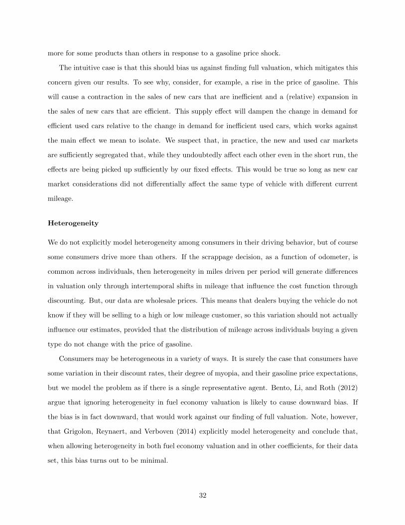
more for some products than others in response to a gasoline price shock.

The intuitive case is that this should bias us against finding full valuation, which mitigates this

concern given our results. To see why, consider, for example, a rise in the price of gasoline. This

will cause a contraction in the sales of new cars that are inefficient and a (relative) expansion in

the sales of new cars that are efficient. This supply effect will dampen the change in demand for

efficient used cars relative to the change in demand for inefficient used cars, which works against

the main effect we mean to isolate. We suspect that, in practice, the new and used car markets

are sufficiently segregated that, while they undoubtedly affect each other even in the short run, the

effects are being picked up sufficiently by our fixed effects. This would be true so long as new car

market considerations did not differentially affect the same type of vehicle with different current

mileage.

Heterogeneity

We do not explicitly model heterogeneity among consumers in their driving behavior, but of course

some consumers drive more than others. If the scrappage decision, as a function of odometer, is

common across individuals, then heterogeneity in miles driven per period will generate differences

in valuation only through intertemporal shifts in mileage that influence the cost function through

discounting. But, our data are wholesale prices. This means that dealers buying the vehicle do not

know if they will be selling to a high or low mileage customer, so this variation should not actually

influence our estimates, provided that the distribution of mileage across individuals buying a given

type do not change with the price of gasoline.

Consumers may be heterogeneous in a variety of ways. It is surely the case that consumers have

some variation in their discount rates, their degree of myopia, and their gasoline price expectations,

but we model the problem as if there is a single representative agent. Bento, Li, and Roth (2012)

argue that ignoring heterogeneity in fuel economy valuation is likely to cause downward bias. If

the bias is in fact downward, that would work against our finding of full valuation. Note, however,

that Grigolon, Reynaert, and Verboven (2014) explicitly model heterogeneity and conclude that,

when allowing heterogeneity in both fuel economy valuation and in other coefficients, for their data

set, this bias turns out to be minimal.

32

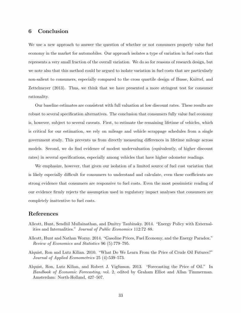
6 Conclusion

We use a new approach to answer the question of whether or not consumers properly value fuel

economy in the market for automobiles. Our approach isolates a type of variation in fuel costs that

represents a very small fraction of the overall variation. We do so for reasons of research design, but

we note also that this method could be argued to isolate variation in fuel costs that are particularly

non-salient to consumers, especially compared to the cross quartile design of Busse, Knittel, and

Zettelmeyer (2013). Thus, we think that we have presented a more stringent test for consumer

rationality.

Our baseline estimates are consistent with full valuation at low discount rates. These results are

robust to several specification alternatives. The conclusion that consumers fully value fuel economy

is, however, subject to several caveats. First, to estimate the remaining lifetime of vehicles, which

is critical for our estimation, we rely on mileage and vehicle scrappage schedules from a single

government study. This prevents us from directly measuring differences in lifetime mileage across

models. Second, we do find evidence of modest undervaluation (equivalently, of higher discount

rates) in several specifications, especially among vehicles that have higher odometer readings.

We emphasize, however, that given our isolation of a limited source of fuel cost variation that

is likely especially difficult for consumers to understand and calculate, even these coefficients are

strong evidence that consumers are responsive to fuel costs. Even the most pessimistic reading of

our evidence firmly rejects the assumption used in regulatory impact analyses that consumers are

completely inattentive to fuel costs.

References

Allcott, Hunt, Sendhil Mullainathan, and Dmitry Taubinsky. 2014. “Energy Policy with External-ities and Internalities.” Journal of Public Economics 112:72–88.

Allcott, Hunt and Nathan Wozny. 2014. “Gasoline Prices, Fuel Economy, and the Energy Paradox.”Review of Economics and Statistics 96 (5):779–795.

Alquist, Ron and Lutz Kilian. 2010. “What Do We Learn From the Price of Crude Oil Futures?”Journal of Applied Econometrics 25 (4):539–573.

Alquist, Ron, Lutz Kilian, and Robert J. Vigfusson. 2013. “Forecasting the Price of Oil.” InHandbook of Economic Forecasting, vol. 2, edited by Graham Elliot and Allan Timmerman.Amsterdam: North-Holland, 427–507.

33

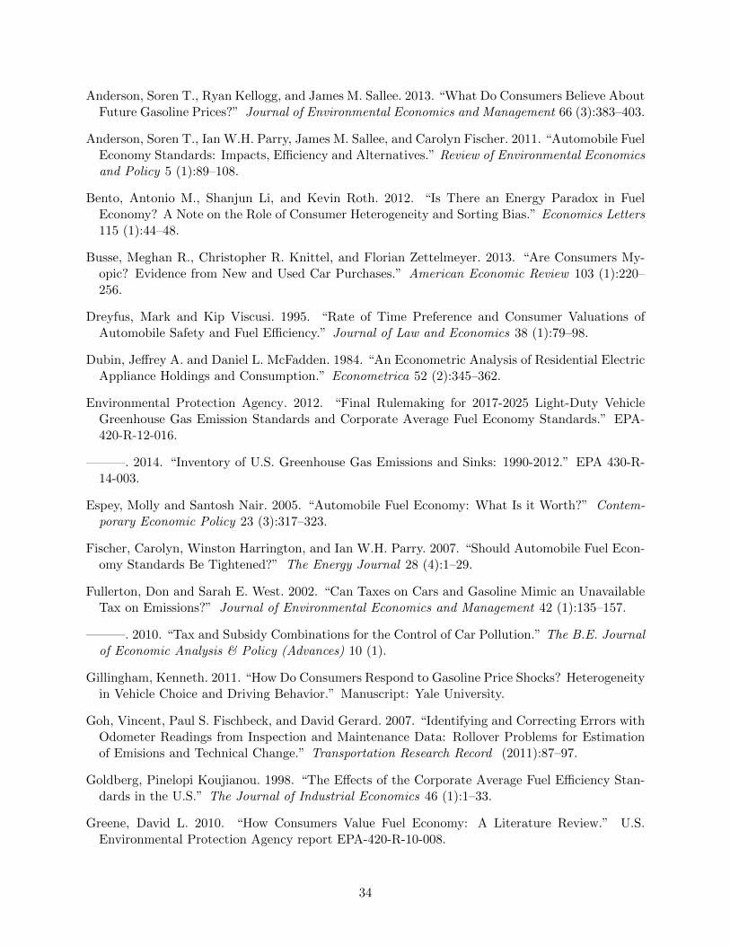
Anderson, Soren T., Ryan Kellogg, and James M. Sallee. 2013. “What Do Consumers Believe AboutFuture Gasoline Prices?” Journal of Environmental Economics and Management 66 (3):383–403.

Anderson, Soren T., Ian W.H. Parry, James M. Sallee, and Carolyn Fischer. 2011. “Automobile FuelEconomy Standards: Impacts, Efficiency and Alternatives.” Review of Environmental Economicsand Policy 5 (1):89–108.

Bento, Antonio M., Shanjun Li, and Kevin Roth. 2012. “Is There an Energy Paradox in FuelEconomy? A Note on the Role of Consumer Heterogeneity and Sorting Bias.” Economics Letters115 (1):44–48.

Busse, Meghan R., Christopher R. Knittel, and Florian Zettelmeyer. 2013. “Are Consumers My-opic? Evidence from New and Used Car Purchases.” American Economic Review 103 (1):220–256.

Dreyfus, Mark and Kip Viscusi. 1995. “Rate of Time Preference and Consumer Valuations ofAutomobile Safety and Fuel Efficiency.” Journal of Law and Economics 38 (1):79–98.

Dubin, Jeffrey A. and Daniel L. McFadden. 1984. “An Econometric Analysis of Residential ElectricAppliance Holdings and Consumption.” Econometrica 52 (2):345–362.

Environmental Protection Agency. 2012. “Final Rulemaking for 2017-2025 Light-Duty VehicleGreenhouse Gas Emission Standards and Corporate Average Fuel Economy Standards.” EPA-420-R-12-016.

———. 2014. “Inventory of U.S. Greenhouse Gas Emissions and Sinks: 1990-2012.” EPA 430-R-14-003.

Espey, Molly and Santosh Nair. 2005. “Automobile Fuel Economy: What Is it Worth?” Contem-porary Economic Policy 23 (3):317–323.

Fischer, Carolyn, Winston Harrington, and Ian W.H. Parry. 2007. “Should Automobile Fuel Econ-omy Standards Be Tightened?” The Energy Journal 28 (4):1–29.

Fullerton, Don and Sarah E. West. 2002. “Can Taxes on Cars and Gasoline Mimic an UnavailableTax on Emissions?” Journal of Environmental Economics and Management 42 (1):135–157.

———. 2010. “Tax and Subsidy Combinations for the Control of Car Pollution.” The B.E. Journalof Economic Analysis & Policy (Advances) 10 (1).

Gillingham, Kenneth. 2011. “How Do Consumers Respond to Gasoline Price Shocks? Heterogeneityin Vehicle Choice and Driving Behavior.” Manuscript: Yale University.

Goh, Vincent, Paul S. Fischbeck, and David Gerard. 2007. “Identifying and Correcting Errors withOdometer Readings from Inspection and Maintenance Data: Rollover Problems for Estimationof Emisions and Technical Change.” Transportation Research Record (2011):87–97.

Goldberg, Pinelopi Koujianou. 1998. “The Effects of the Corporate Average Fuel Efficiency Stan-dards in the U.S.” The Journal of Industrial Economics 46 (1):1–33.

Greene, David L. 2010. “How Consumers Value Fuel Economy: A Literature Review.” U.S.Environmental Protection Agency report EPA-420-R-10-008.

34

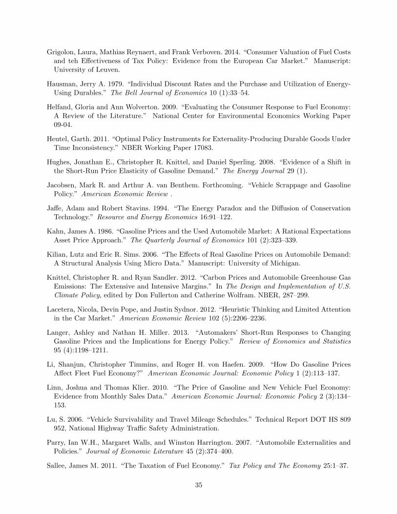
Grigolon, Laura, Mathias Reynaert, and Frank Verboven. 2014. “Consumer Valuation of Fuel Costsand teh Effectiveness of Tax Policy: Evidence from the European Car Market.” Manuscript:University of Leuven.

Hausman, Jerry A. 1979. “Individual Discount Rates and the Purchase and Utilization of Energy-Using Durables.” The Bell Journal of Economics 10 (1):33–54.

Helfand, Gloria and Ann Wolverton. 2009. “Evaluating the Consumer Response to Fuel Economy:A Review of the Literature.” National Center for Environmental Economics Working Paper09-04.

Heutel, Garth. 2011. “Optimal Policy Instruments for Externality-Producing Durable Goods UnderTime Inconsistency.” NBER Working Paper 17083.

Hughes, Jonathan E., Christopher R. Knittel, and Daniel Sperling. 2008. “Evidence of a Shift inthe Short-Run Price Elasticity of Gasoline Demand.” The Energy Journal 29 (1).

Jacobsen, Mark R. and Arthur A. van Benthem. Forthcoming. “Vehicle Scrappage and GasolinePolicy.” American Economic Review .

Jaffe, Adam and Robert Stavins. 1994. “The Energy Paradox and the Diffusion of ConservationTechnology.” Resource and Energy Economics 16:91–122.

Kahn, James A. 1986. “Gasoline Prices and the Used Automobile Market: A Rational ExpectationsAsset Price Approach.” The Quarterly Journal of Economics 101 (2):323–339.

Kilian, Lutz and Eric R. Sims. 2006. “The Effects of Real Gasoline Prices on Automobile Demand:A Structural Analysis Using Micro Data.” Manuscript: University of Michigan.

Knittel, Christopher R. and Ryan Sandler. 2012. “Carbon Prices and Automobile Greenhouse GasEmissions: The Extensive and Intensive Margins.” In The Design and Implementation of U.S.Climate Policy, edited by Don Fullerton and Catherine Wolfram. NBER, 287–299.

Lacetera, Nicola, Devin Pope, and Justin Sydnor. 2012. “Heuristic Thinking and Limited Attentionin the Car Market.” American Economic Review 102 (5):2206–2236.

Langer, Ashley and Nathan H. Miller. 2013. “Automakers’ Short-Run Responses to ChangingGasoline Prices and the Implications for Energy Policy.” Review of Economics and Statistics95 (4):1198–1211.

Li, Shanjun, Christopher Timmins, and Roger H. von Haefen. 2009. “How Do Gasoline PricesAffect Fleet Fuel Economy?” American Economic Journal: Economic Policy 1 (2):113–137.

Linn, Joshua and Thomas Klier. 2010. “The Price of Gasoline and New Vehicle Fuel Economy:Evidence from Monthly Sales Data.” American Economic Journal: Economic Policy 2 (3):134–153.

Lu, S. 2006. “Vehicle Survivability and Travel Mileage Schedules.” Technical Report DOT HS 809952, National Highway Traffic Safety Administration.

Parry, Ian W.H., Margaret Walls, and Winston Harrington. 2007. “Automobile Externalities andPolicies.” Journal of Economic Literature 45 (2):374–400.

Sallee, James M. 2011. “The Taxation of Fuel Economy.” Tax Policy and The Economy 25:1–37.

35

———. 2014. “Rational Inattention and Energy Efficiency.” Journal of Law and Economics57 (3):781–820.

36

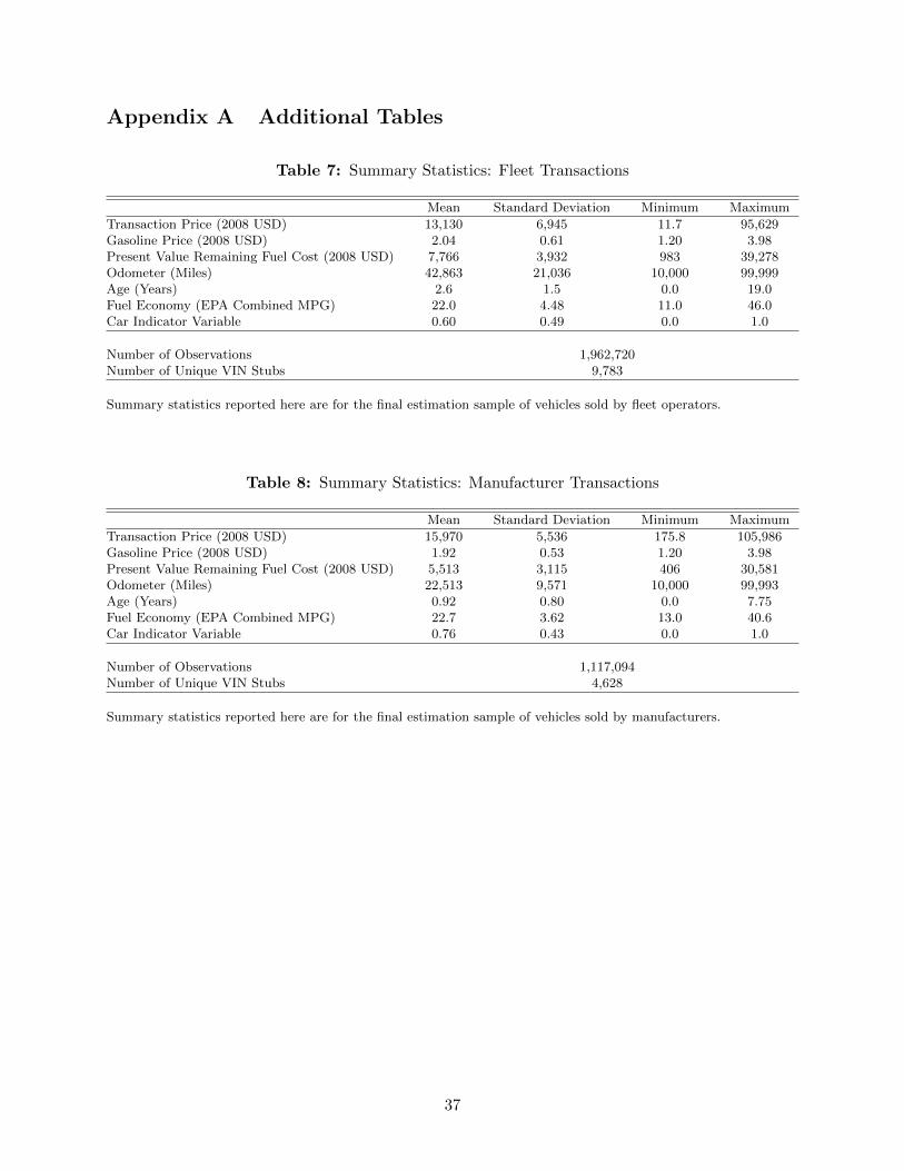
Appendix A Additional Tables

Table 7: Summary Statistics: Fleet Transactions

Mean Standard Deviation Minimum Maximum

Transaction Price (2008 USD) 13,130 6,945 11.7 95,629Gasoline Price (2008 USD) 2.04 0.61 1.20 3.98Present Value Remaining Fuel Cost (2008 USD) 7,766 3,932 983 39,278Odometer (Miles) 42,863 21,036 10,000 99,999Age (Years) 2.6 1.5 0.0 19.0Fuel Economy (EPA Combined MPG) 22.0 4.48 11.0 46.0Car Indicator Variable 0.60 0.49 0.0 1.0

Number of Observations 1,962,720Number of Unique VIN Stubs 9,783

Summary statistics reported here are for the final estimation sample of vehicles sold by fleet operators.

Table 8: Summary Statistics: Manufacturer Transactions

Mean Standard Deviation Minimum Maximum

Transaction Price (2008 USD) 15,970 5,536 175.8 105,986Gasoline Price (2008 USD) 1.92 0.53 1.20 3.98Present Value Remaining Fuel Cost (2008 USD) 5,513 3,115 406 30,581Odometer (Miles) 22,513 9,571 10,000 99,993Age (Years) 0.92 0.80 0.0 7.75Fuel Economy (EPA Combined MPG) 22.7 3.62 13.0 40.6Car Indicator Variable 0.76 0.43 0.0 1.0

Number of Observations 1,117,094Number of Unique VIN Stubs 4,628

Summary statistics reported here are for the final estimation sample of vehicles sold by manufacturers.

37