NBER WORKING PAPER SERIES

DO ENERGY EFFICIENCY INVESTMENTS DELIVER AT THE RIGHT TIME?

Judson P. BoomhowerLucas W. Davis

Working Paper 23097http://www.nber.org/papers/w23097

NATIONAL BUREAU OF ECONOMIC RESEARCH1050 Massachusetts Avenue

Cambridge, MA 02138January 2017

We are grateful to Severin Borenstein, Jim Bushnell, Andrew Campbell, Steve Cicala, Peter Jacobsand seminar participants at Carnegie Mellon, Indiana University, Lawrence Berkeley National Lab,Resources for the Future, Stanford University, UC Berkeley, UC San Diego, UC Santa Cruz, Universityof Chicago, University of Michigan, and the AERE annual meeting for helpful comments and to EllenLin and Matt Woerman for excellent research assistance. This research was supported by the CaliforniaEnergy Commission under EPC-14-026. The authors have not received any financial compensationfor this project nor do they have any financial relationships that relate to this research. The views expressedherein are those of the authors and do not necessarily reflect the views of the National Bureau of EconomicResearch.

NBER working papers are circulated for discussion and comment purposes. They have not been peer-reviewed or been subject to the review by the NBER Board of Directors that accompanies officialNBER publications.

© 2017 by Judson P. Boomhower and Lucas W. Davis. All rights reserved. Short sections of text,not to exceed two paragraphs, may be quoted without explicit permission provided that full credit,including © notice, is given to the source.

Do Energy Efficiency Investments Deliver at the Right Time?Judson P. Boomhower and Lucas W. DavisNBER Working Paper No. 23097January 2017JEL No. D40,Q41

ABSTRACT

Electricity cannot be cost-effectively stored even for short periods of time. Consequently, wholesale electricity prices vary widely across hours of the day with peak prices frequently exceeding off-peak prices by a factor of ten or more. Most analyses of energy-efficiency policies ignore this variation, focusing on total energy savings without regard to when those savings occur. In this paper we demonstrate the importance of this distinction using novel evidence from a rebate program for air conditioners in Southern California. We estimate electricity savings using hourly smart-meter data and show that savings tend to occur during hours when the value of electricity is high. This significantly increases the overall value of the program, especially once we account for the large capacity payments received by generators to guarantee their availability in high-demand hours. We then compare this estimated savings profile with engineering-based estimates for this program as well as a variety of alternative energy-efficiency investments. The results illustrate a surprisingly large amount of variation in economic value across investments.

Judson P. BoomhowerStanford University SIEPR366 Galvez StreetMC: 6015Stanford, CA 94305boomhower@stanford.edu

Lucas W. DavisHaas School of BusinessUniversity of CaliforniaBerkeley, CA 94720-1900and NBERldavis@haas.berkeley.edu

1 Introduction

Unlike most other goods, electricity cannot be cost-effectively stored even for short periods.

Supply must meet demand at all times, or the frequency in the grid will fall outside of

a narrow tolerance band, causing blackouts. In addition, electricity demand is highly

variable and inelastic. As a result, electricity markets clear mostly on the supply side,

with production ramping up and down to meet demand. During off-peak hours electricity

prices tend to be very low. However, during peak hours prices rise substantially, frequently

to two- or three- times the level of off-peak prices. Moreover, there are a small number

of peak hours during the year when prices increase much more, often to ten- or twenty-

times the level of off-peak prices. During these ultra-peak hours generation is operating at

full capacity and there is little ability to further increase supply so demand reductions are

extremely valuable.

These features of electricity markets are well known, yet most analyses of energy-efficiency

policies ignore this variation. When the U.S. Department of Energy (DOE) considers new

appliance energy-efficiency standards and building energy codes, they focus on total energy

savings without regard to when they occur.1 When state utility commissions evaluate

energy-efficiency programs, they focus on total energy savings, typically with little regard

to timing.2 Also, most large-scale energy models including the DOE’s National Energy

Modeling System lack temporal granularity altogether and instead model energy demand

1 For appliance energy standards, see Commercial Package Air Conditioning and Heating Equipmentand Warm Air Furnaces (81 FR 2420, January 15, 2016); Ceiling Fan Light Kits (81 FR 580, January6, 2016); Single Package Vertical Air Conditioners and Heat Pumps (80 FR 57438, September 23, 2015);Commercial Clothes Washers (79 FR 12302, March 3, 2014); Residential Clothes Dryers and Room AirConditioners (76 FR 22454, April 21, 2011); and Incandescent Lamps, Dishwashers, and Other Appliances(DOE 2009, Technical support document: Impacts on the Nation of the Energy Independence and Se-curity Act of 2007). For residential building energy codes, see DOE, “Determination Regarding EnergyEfficiency Improvements in the 2015 International Energy Conservation Code (IECC)”, 80 FR 33250, June11, 2015; and technical support documents cited therein. For commercial building energy codes, see DOE,“Determination Regarding Energy Efficiency Improvements in ANSI/ASHRAE/IES Standard 90.1–2013:Energy Standard for Buildings, Except Low-Rise Residential Buildings”, 79 FR 57900, September 26, 2014.Citations with FR refer to the Federal Register.

2 See, for example, California Public Utilities Commission, “Energy Efficiency Annual Progress Evalu-ation Report”, March 2015; Public Service Commission of Maryland, “The EmPOWER Maryland EnergyEfficiency Act Standard Report of 2015”, April 2015; Massachusetts Energy Efficiency Advisory Council,“2013 Annual Report: Energy Efficiency Sets the Stage for Sustainable, Long-Term Savings”, 2014; North-west Power and Conservation Council, “2014 Achievements: Progress Toward the Sixth Plan’s RegionalConservation Goals”, November 2015; Consortium for Energy Efficiency, “2015 State of the EfficiencyProgram Industry”, March 2016.

1

at the monthly or even annual level. With a few notable exceptions that we discuss later in

the paper, there is surprisingly little attention both by policymakers and in the academic

literature to how the value of energy efficiency depends on when savings occur.

In part, these limitations reflect historical technological constraints. Before smart meters

and other advanced metering infrastructure, it was impossible to measure policy impacts

at the hourly level. The necessary high frequency data simply did not exist, since meters

were only read once per billing cycle. This situation is rapidly changing. Today in the

United States more than 40% of residential electricity customers have smart meters, up

from less than 2% in 2007.3

In this paper we demonstrate the importance of accounting for the timing of energy sav-

ings using novel evidence from a rebate program for energy-efficient air conditioners in

Southern California. We use hourly smart-meter data to estimate the change in electricity

consumption after installation of an energy-efficient air conditioner, and show that savings

tend to occur disproportionately during July and August, and during the hours 3 p.m. to

9 p.m. With hourly data from 6,000+ participants, we are able to precisely characterize

the savings profile both across seasons and hours of the day.

Our estimated time profile of energy savings is similar to ex ante engineering estimates,

but there are several interesting differences. Most importantly, the econometric estimates

indicate peak savings between 6 p.m. and 7 p.m., compared to between 4 p.m. and 5 p.m.

in the engineering estimates. This seemingly small difference has important implications

for electricity markets given growing concern about meeting electricity demand during

the early evening hours as the sun sets and solar generation decreases (see, e.g., CAISO,

2013).

We then use price data from wholesale energy and forward capacity markets to quantify

the economic value of these estimated savings. Savings are strongly correlated with the

value of electricity, making the program 48% more valuable than under a naive calculation

ignoring timing. As we demonstrate, including capacity payments is important in this

calculation. Most of the value of electricity in ultra-peak hours is captured by forward

capacity payments to generators to guarantee their availability.

Finally we compare air conditioning to a much larger set of energy-efficiency investments,

3U.S. Department of Energy, “Electric Power Annual”, Released February 2016, Tables 2.1 and 10.10.

2

both residential and non-residential. Overall, there is a remarkably wide range of value

across investments. Across six major U.S. markets, we find that air conditioning invest-

ments are on average 29% more valuable than under a naive calculation ignoring timing.

For commercial and industrial heat pumps and chillers the “timing premiums” are 29% and

25%, respectively. Other investments like refrigerators and freezers have timing premiums

below 5% because savings are only weakly correlated with value. Lighting also does sur-

prisingly poorly, reflecting that savings occur disproportionately during evening and winter

hours when electricity tends to be less valuable.

These findings have important policy implications. Energy-efficiency is a major focus of

energy policy in the United States and other countries. Electric utilities in the United

States, for example, spent $36 billion on energy-efficiency programs between 2006 and

2015, leading to more than 1.5 million gigawatt hours in reported total electricity savings.4

In addition, the U.S. Federal government has spent $12 billion since 2009 on income tax

credits for residential energy-efficiency investments (Borenstein and Davis, 2015). Virtually

all analyses of these programs have ignored the timing of energy savings.

The paper proceeds as follows. Section 2 provides background about electricity markets and

energy-efficiency. Section 3 describes our empirical application, estimating framework, and

savings estimates. Section 4 then examines the correlation between savings and the value

of electricity, incorporating engineering-based estimated savings profiles from alternative

energy-efficiency investments. Section 5 concludes.

2 Background

2.1 Electricity Markets

Electricity is supplied in most markets by a mix of generating technologies. Wind, solar,

and other renewables are at the bottom of the supply curve with near-zero marginal cost.

Nuclear, coal, and natural gas combined-cycle plants come next, all with low marginal cost.

Higher up the supply curve come generating units like natural gas combustion turbines

and even oil-burning “peaker” plants, which have high marginal costs but low fixed costs.

4Tabulations by the authors based on data from U.S. Department of Energy, Energy Information Ad-ministration, “Electric Power Annual”, 2012 (Tables 10.2 and 10.5) and 2015 (Tables 10.6 and 10.7).Expenditures are reported in year 2015 dollars.

3

Beyond that the supply curve for electricity is perfectly vertical, reflecting the maximum

total generating capacity.

This mix is necessary because electricity cannot be cost-effectively stored. Demand for

electricity is price inelastic and varies widely across hours. Consequently, electricity mar-

kets clear primarily on the supply side, with generation ramping up and down to meet

demand. During off-peak hours, the marginal generator typically has a relatively low or

even zero marginal cost. But during peak hours the marginal generator has a much higher

marginal cost. Even within natural gas plants, for example, marginal costs can vary by a

factor of two or more. There are also typically a small number of ultra-peak hours each

year in which demand outstrips the maximum capacity of generation, leading the market

to clear on the demand side and resulting in prices that can spike to many times any plant’s

marginal cost.

An immediate implication of these features of electricity markets is that the value of demand

reductions varies widely across hours. Most buyers do not see real-time prices (Borenstein,

2005; Borenstein and Holland, 2005; Holland and Mansur, 2006). Instead, many electric

utilities have implemented demand response programs, optional critical peak pricing tariffs,

and other policies aimed at curbing electricity demand during ultra-peak periods.

Wholesale energy prices provide a measure of how the value of electricity varies across

hours. In an idealized “energy-only” market, this would be the complete measure of value

and the only signal power plant owners would need when deciding whether to enter or

exit. In a competitive market in long-run equilibrium, the number of power plants would

be determined by price competition and free entry. Additional plants would be built until

the average price across all hours just equaled average cost. In such a market, the hourly

wholesale electricity price represents the full value of avoided electricity consumption in

any given hour.

The reality of electricity markets, even “deregulated” ones, is more complex. In many

markets the amount of power plant capacity is set by regulation. Because price cannot

instantaneously clear the market, there is a risk of excess demand in peak periods, poten-

tially leading to blackouts or costly equipment damage.5 Regulators set minimum “reserve

5In principle, household-level interruptible tariffs could solve this problem but they have historicallybeen infeasible (although this may be changing with new technologies). Some electricity markets alsoinclude price caps, which can depress energy market revenues and create an additional rationale for marketintervention.

4

margins” (generation capacity in excess of expected peak demand) that reduce the risk

of electricity shortages below some target level, such as one event every ten years. These

reserve margin requirements are implemented through dedicated capacity markets where

generators commit to make their plants available to sell power during future periods.6 The

equilibrium capacity price just covers the shortfall between expected energy market rev-

enues and total cost for the marginal new power plant at the desired reserve margin. In

the US, much of the price signal for new investment in electricity markets is communicated

through capacity markets.

It is important to take capacity markets into account when measuring how the value of

electricity varies across hours. As we will show later, considering only wholesale electricity

prices (“energy prices”) tends to systematically understate the degree to which the value

of electricity varies across hours. Although the total size of capacity markets tends to

be much smaller than the electricity markets themselves, the amounts of these payments

depend only on the highest few demand hours each year. In the extreme, consider a

“peaker” plant which receives a significant capacity payment for being available to be used

only a very small number of hours each year. Accounting for these capacity payments

increases the marginal cost of electricity in this handful of hours enormously, to potentially

50+ times the hourly prices in the energy market.

Finally, another important feature of electricity markets is large externalities. These exter-

nal costs of energy production also vary across hours and across markets. Callaway et al.

(2015) use site-level data on renewables generation and engineering estimates of the hourly

load profiles for lighting to show how the total social value of those resources varies across

U.S. markets. There are large regional differences with particularly large external damages

in the Midwest. In this paper, however, we limit our focus to private energy cost savings.

Perhaps contrary to popular expectation, the large majority of the stated benefits from

most energy-efficiency policies come from reduced private energy costs (Gayer and Viscusi,

6For example, the California Public Utilities Commission adopts a forecast of peak demand for eachmonth and requires utilities to enter into “resource adequacy” contracts to ensure that they can meet 115%of this demand. The payments in these contracts are very high in months when peak electricity demand isexpected to be near total system capacity. As we show later, reducing forecast peak demand in August byone megawatt-hour avoids thousands of dollars in resource adequacy payments, which is many times theenergy market price in those hours. For more discussion of capacity markets see Bushnell (2005); Cramtonand Stoft (2005); Joskow (2006); Joskow and Tirole (2007); Alcott (2013). Many electricity markets alsoprovide additional payments for frequency regulation and other ancillary services, but these payments tendto be smaller than capacity payments and energy-efficiency is less well-suited for providing these services.

5

2013). For example, nine new standards promulgated by the DOE in 2016 achieve a total

present value of $76 billion in energy cost savings, vs. $28 billion in avoided CO2 emissions

and $5 billion in avoided NOx emissions.7 That is, more than two-thirds of the benefits

come from private energy cost savings. Moreover, the hourly variation in external costs is

small relative to the hourly variation in electricity prices and capacity values. Private value

varies across hours by a factor of ten or more, while emission rates vary only by about a

factor of two between fossil-fuel plants. For both of these reasons, in this paper we focus

exclusively on private costs and refer readers interested in externalities to Callaway et al.

(2015).

2.2 Energy Efficiency

Electricity is a widely-used input, both in manufacturing and in the production of cooling,

lighting, refrigeration, and other household services. Energy efficiency is the rate at which

energy inputs are converted into these outputs. Households and firms can choose to improve

energy efficiency through a variety of (usually capital-intensive) investments. The ultimate

level of investment in energy efficiency depends on capital costs, energy prices, discount

rates, and other factors.

Governments intervene in energy efficiency to reduce peak demand, increase “energy se-

curity”, and reduce externalities from energy consumption. Most economists argue for

better-targeted policies, such as emissions taxes and real-time pricing of electricity, but

these are politically unpopular. Instead, there are a growing number of policies aimed at

increasing energy efficiency. This paper fits into a recent literature that emphasizes the im-

portance of rigorous ex-post analyses of these programs using real market outcomes (Davis

et al., 2014; Fowlie et al., 2015; Allcott and Greenstone, 2015). In this paper we extend

that work to include the hourly shape of demand reductions.

The vast majority of existing economic analyses of energy efficiency have focused on total

7We made these calculations based on the nine new standards listed in DOE’s February, 2016 andAugust, 2016 semi-annual reports to Congress. The individual rulemakings are Single Package Vertical AirConditioners and Heat Pumps (80 FR 57438, September 23, 2015); Ceiling Fan Light Kits (81 FR 580,January 6, 2016); Refrigerated Beverage Vending Machines (81 FR 1028, January 8, 2016); CommercialPackage Air Conditioning and Heating Equipment and Warm Air Furnaces (81 FR 2420, January 15, 2016);Residential Boilers (81 FR 2320, January 15, 2016); Commercial and Industrial General Pumps (81 FR4368, January 26, 2016); Commercial Prerinse Spray Valves (81 FR 4748, January 27, 2016); BatteryChargers (81 FR 38266, June 16, 2016); and Dehumidifiers (81 FR 38338, June 31, 2016).

6

savings, rather than on when these savings occur (see e.g. Dubin et al. (1986); Metcalf

and Hassett (1999); Davis (2008); Arimura et al. (2012); Barbose et al. (2013); Davis et al.

(2014); Fowlie et al. (2015)). An important exception is Novan and Smith (2016) which uses

hourly data from a similar energy-efficiency program to illustrate important inefficiencies

with current retail rate designs for electricity. Our paper in contrast is much more focused

on the timing of energy savings and how this impacts the total value of energy-efficiency

investments.

Like academic research, regulatory analyses conducted during the design and evaluation of

energy efficiency policies have also overwhelmingly ignored the timing of savings. Minimum

efficiency standards are probably the most pervasive form of government intervention in

energy efficiency. There are standards for 40+ categories of residential and commercial

technologies in the United States. Analyses of these standards focus on total energy savings,

ignoring timing. Meyers et al. (2015), for example, calculate energy costs savings for U.S.

federal energy-efficiency standards using average annual energy prices, thus ignoring any

potential correlation between savings and the value of electricity. They find that U.S.

energy-efficiency standards saved households and firms $60 billion in 2014. The DOE

performs additional economic analyses every time a new U.S. standard is implemented but

again, the emphasis is on total energy savings without regard to when these savings occur

(see references in Footnote 1).

Another major category of policies are subsidies for energy-efficient technologies. This

includes federal and state income tax credits for energy efficiency investments, sales tax

holidays, and, at the state level, utility-sponsored rebates and upstream manufacturer

incentives. Most state utility commissions require these programs to be evaluated by third-

party analysts. Although thousands of studies have been performed looking at subsidy

programs, the vast majority focus on total energy savings (for example, see references

cited in Footnote 2).8

There are exceptions. California requires that proposed utility-sponsored energy-efficiency

programs be evaluated against engineering models of hourly electricity values before pro-

grams are implemented. California’s Title 24 building efficiency standards also explicitly

8Some evaluations acknowledge timing in a very coarse way by reporting the effect of programs onannual peak demand. This recognizes the importance of physical generation constraints, but ignores thelarge hour-to-hour variation in the value of electricity in all other hours. This approach also does not assignan economic value to peak load reductions.

7

consider time value. Some recent federal energy efficiency standards consider seasonal

differences in savings values, but still ignore the enormous variation within seasons and

across hours of the day.9 In addition, while the vast majority of third-party analyses of

energy-efficiency programs ignore the timing of savings, a notable exception is Evergreen

Economics (2016), which compares random coefficients versus alternative models for esti-

mating hourly savings for several California energy-efficiency programs.

3 Empirical Application

For our empirical application, we focus on a residential air conditioner program in South-

ern California. Section 3.1 briefly describes the key features of the program, Section 3.2

provides graphical evidence on average electricity savings, Sections 3.3 and 3.4 plot savings

estimates by daily temperature and hour-of-day, respectively, and then Section 3.5 reports

regression estimates.

3.1 Program Background

Our empirical application is an energy-efficiency rebate program offered by Southern Cal-

ifornia Edison (SCE), a major investor-owned utility. SCE is one of the largest electric

utilities in the United States, providing electricity service to 14 million people. SCE pur-

chases power in the wholesale electricity market operated by the California Independent

System Operator and sells it to residential, commercial, and industrial customers.

The program is known as the Quality Installation Program. It provides incentives of up to

$1,100 to households that install an energy-efficient central air conditioner. This program

is an excellent empirical setting in which to examine the time-specific value of energy

savings. Air conditioning is responsible for 10% of average residential electricity use and

15% of average commercial electricity use in California (California Energy Commission,

2012). California’s investor-owned utilities, under the direction of the California Public

Utilities Commission, have devoted significant resources to programs aimed at reducing

energy use from air conditioning. More broadly, air conditioning is projected to be one of

the fastest growing uses of electricity worldwide (see, e.g., Davis and Gertler, 2015). This

9For example, the 2016 standards for Ceiling Fan Light Kits (81 FR 580, January 6, 2016).

8

large demand for air conditioning is concentrated in certain seasons of the year and hours

of the day.

The Quality Installation Program is administered similarly to most energy-efficiency sub-

sidy programs in the United States. As with other programs, the household claims the

rebate through the mail after the new air conditioner is installed. And as with other pro-

grams, the state utility commission compensates SCE for running the program by allowing

the utility to pass on costs to ratepayers in the form of higher electricity prices. The Quality

Installation Program includes an additional focus on proper installation of the new sub-

sidized central air conditioner, which can further improve energy performance (California

Public Utilities Commission, 2011).

The data consist of detailed information about program participants and hourly electricity

consumption records. Our main empirical analyses are based on 6,000+ households who

participated in the program between January 2012 and April 2015. The online appendix

provides additional details, descriptive statistics, and results from alternative specifications

including analyses which incorporate data from non-participating households.

3.2 Event Study

We first present graphical evidence on average energy savings in the form of an event study

figure. This evidence motivates the more detailed analyses that follow and confirms that the

observed changes in electricity consumption coincide with the timing of new air conditioner

installation. In constructing these figures we exploit the natural variation in the timing of

program participation to control for trends in electricity consumption, weather, and other

time-varying factors.

Figure 1 describes the effect of new air conditioner installation on electricity consumption

during the summer and winter, respectively. The horizontal axis is the time in years before

and after installation, normalized so that the year of installation is equal to zero. The figure

plots estimated coefficients and ninety-fifth percentile confidence intervals corresponding

to event time indicator variables from the following regression,

yit =

4∑k=−4

αk1[τit = k]it + ωct + εit. (1)

9

The dependent variable yit is average hourly electricity consumption for household i in year

t and τ denotes the event year defined so that τ = 0 is the exact year in which the new air

conditioner was installed, τ = −3 for three years before, τ = 3 for three years after, and so

on. We do not include an indicator variable for the year before installation (τ = −1), so

the other coefficients are measured relative to that year. We include year by climate zone

fixed effects, ωct, to remove the effect of annual changes in average electricity consumption

in each climate zone due to weather and other time-varying factors.

For summer, we estimate this regression using July and August data from 2012 to 2015

collapsed to the year-by-household level. The sample includes households who installed new

air conditioners between January 2012 and April 2015. We drop data from installations

that occurred during August, September, and October to ensure that participants did not

have new air conditioners during the zero-year summer. This exclusion is for the event

study figure only and these installations are included in all subsequent analyses.

The event study figure for summer shows a sharp decrease in electricity consumption in the

year in which the new air conditioner is installed. The magnitude of the decrease is about

0.2 kilowatt hours per hour. A typical LED lightbulb uses about 10 watts, so this decrease

is equivalent to shutting off 20 LEDs. Electricity consumption is otherwise approximately

flat, both during the four years before and during the four years after.

The event study figure for winter was constructed in exactly the same way but using data

from January and February, and excluding data from installations that occurred during

February, March, or April. As expected, winter consumption is essentially unchanged after

the new air conditioner is installed. This is reassuring because it suggests that the sharp

drop in electricity consumption during summer is indeed due to the new air conditioner

and not some other unrelated change in household appliances or behavior.10

These event study figures and estimates in later sections measure the electricity savings

from a new air conditioner installation. This is different, however, from the causal effect

of the rebate program. Many participants in energy-efficiency programs are inframarginal,

getting paid to do what they would have done otherwise (Joskow and Marron, 1992).

Measuring the causal impact also requires figuring out how the program changed the type

10These estimates of aggregate program impact are quantitatively similar to estimates in SCE-sponsoredEvergreen Economics (2016) based on a random coefficients model. The Evergreen study estimates programimpacts for this program using a much smaller number of homes, and also estimates savings for two otherCalifornia energy-efficiency programs.

10

of appliances that were purchased. In the extreme case in which all participants are in-

framarginal, a program may have no causal impact whatsoever, even while the savings

from an investment are large. Recent studies have used regression discontinuity and other

quasi-experimental techniques to attempt to tease out these causal effects and perform

cost-benefit analysis (Boomhower and Davis, 2014; Houde and Aldy, Forthcoming).

3.3 Impacts by Local Temperature

As another validity test, we next examine the relationship between energy savings and

daily outdoor temperature. A potential concern in our application is that participating

households might have experienced other changes at the same time they installed a new

air conditioner. For example, program take-up might coincide with a home remodel or the

arrival of a new baby, both of which would affect electricity consumption. However, air

conditioning has a very particular pattern of usage that we can use to validate our esti-

mates. Unlike other energy-using durable goods, air conditioner usage is highly correlated

with temperature. Thus, we can validate our empirical approach by confirming that our

estimated savings are large on hot days and near zero on mild days.

We use daily mean temperature data at the four kilometer grid cell level from the PRISM

Climate Group (PRISM Climate Group, 2016). Figure 2 plots estimated electricity savings

against daily mean temperature for each household’s nine-digit zip code. We report re-

gression coefficients for 22 different temperature bins interacted with an indicator variable

for after a new air conditioner is installed. So, for example, the left-most marker reports

the effect of a new air conditioner on days when the temperature is below 40 degrees

Fahrenheit.

On mild days, between 50 and 70 degrees Fahrenheit, estimated energy savings are zero

or not statistically distinguishable from it. The lack of consumption changes on these

days implies that participants are not simultaneously changing their stock or usage of

refrigerators, lighting, or other appliances. From 70 to 100+ degrees, there is a steep,

continuous relationship between temperature and energy savings, as expected from a new

air conditioner. Air conditioner usage is largest on the hottest days, so energy-efficiency

gains have the largest effect on these days. There is also a small decrease in consumption

on days below 50 degrees following air conditioner replacement. This may be explained by

improvements to ductwork, insulation, thermostats, or other HVAC-related upgrades that

11

could in some cases occur as part of a central air conditioner replacement.

3.4 Hourly Impacts by Season

Figure 3 plots estimated electricity savings by hour-of-day. We plot separate estimates for

summer and non-summer months. The coefficients and standard errors for this figure are

estimated using 48 separate least squares regressions. Each regression includes electric-

ity consumption for a single hour-of-the-day and either summer- or non-summer months.

For example, for the top left coefficient the dependent variable is average electricity con-

sumption between midnight and 1 a.m. during non-summer months. All regressions are

estimated at the household-by-week level and control for week-of-sample by climate zone

and household by month-of-year fixed effects.

The figure reveals large differences in savings across seasons and hours. During July and

August there are large energy savings, particularly between noon and 10 p.m. Savings

reach their nadir in the summer at 6 a.m. which is typically the coolest time of the day.

During non-summer months savings are much smaller, less than 0.05 kilowatt hours saved

on average per hour, compared to 0.2 to 0.3 kilowatt hours saved on average per hour

during July and August.

3.5 Regression Estimates

Finally, we turn to a regression framework for characterizing the distribution of energy

savings across hours of the day and months of the year. Our regression equation can be

described as follows,

yith = βhm1[New Air Conditioner]it1[hour/month]hm + γihm + ωth + εith. (2)

Here yith is electricity consumption by household i during week-of-sample t and hour-of-

day h, measured in kilowatt hours. We estimate the model in levels because our pri-

mary interest is in the number and timing of kilowatt hours saved. The indicator variable

1[New Air Conditioner]it, is equal to one for participating households after they have in-

stalled a new air conditioner. Installation dates vary, allowing us to compare households

who have already installed a new air conditioner to households who have not. The main

12

covariates of interest are a set of interaction terms between this indicator variable and a

vector of indicator variables 1[hour/month] for each hour-of-day (h) by month-of-year (m)

pair. For example, one pair is 1:00-2:00 p.m. during November. We estimate 288 separate

β coefficients, each equal to the average change in hourly electricity consumption for a

particular hour-of-day and month-of-year.

All specifications include household by hour-of-day by month-of-year fixed effects, γihm.

That is, for each household we include 288 separate fixed effects that allow for differing

household-level average consumption over the day and across the year. This allows for rich

heterogeneity across households in typical seasonal electricity usage.

All specifications also include week-of-sample by hour-of-day fixed effects ωth. This con-

trols flexibly for territory-wide trends in electricity consumption. These fixed effects absorb

average trends caused by weather variation or secular trends in household electricity con-

sumption. Some specifications include, instead, separate week-of-sample by hour-of-day

fixed effects for each of 8 climate zones. This richer specification controls for climate-zone

specific variation in weather, as well as differential trends across climate zones. This is

potentially important because there are large climatological and demographic differences

between California’s coastal and inland areas. Finally, the error term εith captures unob-

served determinants of consumption across periods.

Table 1 reports estimates from three different specifications. For each specification we

report average annual energy savings per household in kilowatt hours per year. Standard

errors are clustered to allow for arbitrary error correlations at the nine-digit zip code

level.

In columns (1) and (2) the implied annual savings per household are 375 and 358 kilowatt

hours per year, respectively. The difference between these two specifications is that the

latter adds the richer set of time fixed effects. Finally, in column (3) we restrict the

estimation sample to exclude, for each household, the eight weeks prior to installation.

This might make a difference if an old air conditioner was not working or if the installation

date was recorded incorrectly. The estimates are somewhat larger in column (3) but overall

the average savings are similar across the three columns.

Prior to installing a new air conditioner, program participants consumed an average of

9,820 kilowatt hours annually, so this is a 4.5% decrease in household consumption. A

typical central air conditioner (3 ton, 13 SEER) in this region uses about 4,237 kilowatt

13

hours per year, so the savings represent a 10% decrease in annual electricity consumption

for air conditioning. This is broadly similar to, but slightly less than, what would be

expected based on a simple engineering prediction. For example, a Department of Energy

calculator shows that ignoring rebound and other factors a typical central air conditioner

upgrade in Los Angeles saves 565 kilowatt hours per year.11

For computational reasons, we estimate all of these regressions using weekly average con-

sumption at the household by hour-of-day level. Estimation with the hourly microdata is

computationally demanding and does not yield different estimates. Using hourly micro-

data, household by month-of-year by hour-of-day fixed effects, hour-of-sample by climate

zone fixed effects, and the sample exclusions in Column (3), the estimate of annual program

savings is 442 kilowatt hours per year.

4 The Value of Energy Efficiency

In this section we show that the value of electricity varies substantially across hours and we

demonstrate the importance of accounting for this variation when valuing energy-efficiency

investments. We start by showing data on wholesale energy prices and capacity values

(Section 4.1). Then, with the empirical application from the previous section, we measure

the correlation between electricity savings and the value of electricity (Section 4.2) and we

quantify the average value of savings (Section 4.3). With this proof of concept completed,

we then turn to engineering estimates from a broader set of energy-efficiency investments.

We show that the time profile differs significantly between investments (Section 4.4) and

that these different profiles imply large differences in value (Section 4.5).

4.1 The Value of Electricity in U.S. Markets

Figure 4 plots hourly wholesale electricity prices and capacity values for two months-of-year

(February and August) and for two major U.S. electricity markets (California/CAISO and

Texas/ERCOT). We selected February and August because they tend to be relatively low-

11Typical central air conditioner electricity usage and predicted savings are from Energy Star Pro-gram, “Life Cycle Cost Estimate for 1 ENERGY STAR Qualified Central Air Conditioner(s)”, 2013.https://www.energystar.gov/. These statistics assume replacement of a 3-ton 13 SEER unit with 3-ton15 SEER without programmable thermostat before or after.

14

and high-demand months but adjacent months look similar. For each market we report

average prices by hour-of-day for 2011 through 2015. The energy and capacity price data

that we use come from SNL Financial and are described in the online appendix. We include

ERCOT as a benchmark for our California capacity value estimates; because ERCOT has

no capacity market, the full value of electricity is encoded in hourly energy prices.

For California, the figures plot average wholesale energy prices as well as four alternative

measures of capacity value. As discussed in Section 2.1, capacity payments are made

to electricity generators to remain open and available, thereby ensuring desired reserve

margins. Capacity costs are zero or close to it during off-peak hours because electricity

demand can be easily met by existing inframarginal generators (plants that are not close

to the margin between staying in the market and exiting). However, during peak hours

large capacity payments are required to ensure desired reserve margins. ERCOT has no

capacity market and, not coincidentally, has higher energy market prices than California

during peak hours.

In California, generation capacity is procured at the monthly level (that is, capacity con-

tracts obligate generators to be available every hour of one month). In order to value

energy savings in a given hour, we need to allocate these monthly capacity prices across

individual hours. We do this in several different ways and report the results of each. In

the first approach, we use hourly load data to calculate the hour-of-the-day with the high-

est average load each month. We then assign the capacity contract price for that month

entirely to that hour-of-the-day. This means dividing the monthly contract price by the

number of days in the month, and assigning the resulting amount to the peak hour. In

other specifications, we divide the capacity contract price evenly over the top two or three

hours-of-the-day with the highest load each month. The final approach treats each day of

load data as a single observation of daily load shape in a given month. We calculate the his-

torical likelihood that each hour-of-the-day was the daily peak hour, and allocate monthly

capacity prices to hours of the day proportionally according to these probabilities.

Incorporating capacity values substantially increases the value of electricity during peak

periods. In California during August, for example, capacity values increase the value of

electricity during peak evening hours to between $200 and $600 per megawatt hour. And,

overall, the pattern is very similar across the four approaches for allocating capacity value

across hours. As expected, allocating the entire capacity value to the single highest-load

15

hour results in the highest peak, though the other approaches have similar shapes. In

addition, the general shape of the capacity-inclusive hourly values for California matches

the shape in Texas, providing some reassurance that our allocation strategy recovers the

price shape that would exist in an energy-only market.12 The value of electricity in Texas

surges in August to $200+ during the late afternoon, considerably higher than the marginal

cost of any generator.

An alternative approach to valuing capacity would be to use engineering estimates for the

cost of new electricity generating equipment like a natural gas combustion turbine plant.

This would address the concern that capacity markets may not be in long-run equilibrium,

and thus may not reflect the true long-run cost of capacity. Some market participants

have argued, for example, that the recent influx of renewables into U.S. electricity markets

has pushed capacity market prices down below long-run equilibrium levels. If this is the

case then over time entry and exit decisions should lead to increased capacity prices and

it would be straightforward to repeat our calculations with updated data. Larger capacity

prices would lead to larger variation in economic value between off-peak and peak, thus

strengthening our central findings.

The calculations which follow also account for line losses in electricity transmission and

distribution. In the United States, an average of 6% of electricity is lost between the point

of generation and the point of consumption (DOE, 2016, Table 7.1), so 1.0 kilowatt hour

in energy savings reduces generation and capacity requirements by 1.06 kilowatt hours.

Line losses vary over time by an amount approximately proportional to the square of

total generation. We incorporate these losses explicitly following Borenstein (2008) and, in

practice, they range from 4.4% during off-peak periods to 8.4% during ultra-peak periods.

Incorporating line losses thus further increases the variation in economic value between

off-peak and peak.

4.2 Correlation between Savings and Value

Figure 5 shows the correlation between energy savings and the value of energy. Panel A

compares hourly average energy savings to energy prices only. Panel B compares the same

savings estimates to the sum of energy and capacity values. Each marker in each plot

12We return to this point later, when we show that valuing energy savings using the Texas price shapeyields similar results to our approach using California energy and capacity prices.

16

corresponds to an hour-of-day by month-of-year pair (for example, 1:00–2:00 p.m. during

November). The vertical axes show average hourly energy savings. These are the 288 β

coefficients from estimating Equation 2. In Panel A, the horizontal axis shows average

wholesale energy prices from California for 2010–2014. In Panel B, the horizontal axis

shows energy and capacity values, using the probabilistic allocation method for capacity

prices described in Section 4.1.

Several facts are apparent in Panel A. First, the summer months include many more high-

price realizations than the winter months. We use blue markers to indicate April through

September, and the number of intervals with energy prices above $40 per MWh is clearly

higher during these summer months. Second, this energy-efficiency investment delivers

much larger savings in the summer. We saw this before in Figure 3, with average savings

in excess of 0.1 kilowatt-hours per hour in many summer hours.

The figure also includes least-squares fitted lines for April–September (in red) and October–

March (in yellow). The fitted line for summer slopes steeply upward. In the top panel,

predicted savings when energy prices are $55/MWh are twice as large as predicted savings

at $35/MWh. The fitted line for winter, however, is essentially flat. This energy-efficiency

investment delivers essentially zero electricity savings in all hours during the winter, so

there is little correlation between savings and prices.

The same patterns are apparent in Panel B. However, this panel emphasizes the impor-

tance of accounting for hourly capacity values. There are a few ultra-peak hours in the

summer when generation capacity is extremely valuable, and the value of energy surges

to above $200/MWh. Air conditioner investments deliver above-average savings in all of

these hours.

4.3 Quantifying the Value of Energy Savings

Table 2 quantifies the value of the energy savings from this investment. We report estimates

using five alternative approaches for valuing electricity. In column (1) we ignore capacity

values and use wholesale energy prices only. For each hour-of-day and month-of-year pair,

we multiply our estimate of electricity savings in that period by the average wholesale price

in the California market in that period. Summing up these hourly values across all days

of the year gives the annual value of electricity savings. Dividing total annual value by

17

total annual savings gives the average value of each megawatt hour saved, which is what

we report in Row (A) of the table. Under this calculation that accounts for timing, the

average value of savings is $45 per megawatt hour. This is 17% higher than the naive value

estimate using average annual prices and ignoring timing, as in Row (B).

In columns (2) through (5) we incorporate capacity values. Each column takes a different

approach to allocating monthly capacity payments across hours of the day, as described

in Section 4.1 and shown graphically in Figure 4. Incorporating capacity values signifi-

cantly increases the value of air conditioning investments to $68 per megawatt hour. This

reflects the positive correlation between electricity savings and peak hours. Air condition-

ing investments save electricity during the hours-of-day and months-of-year when large

capacity payments are needed to ensure that there is sufficient generation to meet demand.

The naive calculation that ignores timing greatly understates these capacity benefits. The

naive estimate in Row (B) increases only modestly from $39 per megawatt hour to $46 per

megawatt hour after including capacity value. This reflects the fact that most hours have

zero capacity value, so while a few peak hours have capacity values well above $100 per

megawatt-hour the average across the year is only about $6.50 per megawatt hour.

Exactly how we account for capacity values has little impact, changing the estimated timing

premium only slightly across Columns (2) through (5). This is because the estimated

energy savings are similar during adjacent hours, so spreading capacity costs across more

peak hours does not significantly impact the estimated value of savings. In the results that

follow we use the “top 3 hours” allocation (Column (4)) as our preferred measure, but

results are almost identical using the other allocation methods.13

13Results are also similar using alternative specifications that: 1) distinguish between weekdays and week-ends/holidays, or 2) compare to load-weighted average prices. In the first of these, we account for weekends(including holidays) by estimating twice as many coefficients (576), one for each hour-of-day, month-of-year,and weekend or weekday combination. Savings are then valued using weekend- and weekday-specific hourlywholesale prices. Capacity values are assigned to weekdays only, consistent with the significantly higherlevel of net system load. This more complicated specification yields quite similar results, with a timingpremium of 46% compared to 48% in the baseline specification. In the second of these, we compare our mainestimates to load-weighted average prices instead of simple average prices. The load weights are calculatedusing hourly CAISO load from SNL. The timing premium relative to load-weighted average prices is 39%.

18

4.3.1 How Might These Values Change in the Future?

Air conditioners are long-lived investments, so it is also worth considering how the as-

sociated timing premiums could change in the future. Environmental policies that favor

renewable energy technologies are expected to cause significant changes in electricity mar-

kets. California, for example, has a renewable portfolio standard which requires that the

fraction of electricity sourced from renewables increase to 33% by 2020 and 50% by 2030.

These high levels of renewables penetration, and, in particular, solar generation, make

electricity less scarce during the middle of the day, and more valuable in the evening after

the sun sets (CAISO, 2013). The expected steep increase in net load during future evening

periods has prompted concern among grid managers and policymakers.

To examine how this altered price shape could affect the value of energy efficiency, we

performed a sensitivity analysis using forecast prices and load profiles for California in

2024 from Denholm et al. (2015).14 The authors provided us with monthly energy prices

by hour-of-day, and net load forecasts by hour-of-day and season for a scenario with 40%

renewable penetration. We calculated future capacity values by allocating current monthly

capacity contract prices over the three highest net load hours of day in each future month.

Under these assumptions, the timing premium increases from 48% to 74%. Air conditioning

efficiency improvements are even more valuable in this future scenario because increased

solar penetration shifts peak prices further into the late afternoon and early evening, when

energy savings are largest.

This estimate should be interpreted with caution. Predicting the future requires strong

assumptions about electricity demand, natural gas prices, the deployment of electricity

storage, and other factors. This calculation does, however, show how predicted future

prices can be incorporated into this framework for evaluating potential impacts.

4.4 Savings Profiles for Selected Investments

We next bring in engineering estimates of hourly savings profiles for air conditioning and a

wide variety of other energy-efficiency investments. We compare the engineering estimates

14In related work, Martinez and Sullivan (2014) uses an engineering model to examine the potential forenergy efficiency investments to reduce energy consumption in California from 4:00 p.m. to 7:00 p.m. onMarch 31st (a typical Spring day), thereby mitigating the need for flexible ramping resources.

19

for air conditioning to our econometric estimates. Then we use the engineering estimates

for other investments to explore more broadly the question of whether energy efficiency

delivers at the right time. The engineering estimates that we use come from the Database

for Energy Efficient Resources (DEER), a publicly-available software tool developed by the

California Public Utilities Commission (CPUC).15 These are ex ante estimates of energy

savings, constructed using weather data and engineering information on the technological

characteristics of the different technologies.

Figure 6 compares our econometric estimates with engineering estimates for residential air

conditioning investments in this same geographic area. Since our interest is in when savings

occur, both panels are normalized to show the share of total annual savings that occur in

each month and hour (Section 3.5 includes a comparison of total savings amounts). The

two savings profiles are broadly similar, but there are interesting differences. First, the

econometric estimates indicate peak savings later in the evening. The engineering-based

savings estimates peak between 4 p.m. and 5 p.m., while the econometric estimates peak

between 6 p.m. and 7 p.m. This difference is important and policy-relevant because of

expected future challenges in meeting electricity demand during sunset hours, as discussed

in the previous section.

There are other differences as well. The econometric estimates show a significant share of

savings during summer nights and even early mornings, whereas the engineering estimates

show savings quickly tapering off at night during the summer, reaching zero at midnight.

It could be that the engineering estimates are insufficiently accounting for the thermal

mass of California homes and how long it takes them to cool off after a warm summer day.

The econometric estimates also show greater concentration of savings during the warmest

months. Both sets of estimates indicate July and August as the two most important

months for energy savings. But the engineering estimates indicate a significant share of

savings in all five summer months, and a non-negligible share of savings during winter

months. In contrast, the econometric estimates show that almost all of the savings occur

June through September with only modest savings in October and essentially zero savings

in other months.

15The DEER is used by the CPUC to design and evaluate energy-efficiency programs administered byCalifornia investor-owned utilities. For each energy-efficiency investment the DEER reports 8,760 numbers,one for each hour of the year. We use the savings profiles developed in 2013/2014 for the Southern CaliforniaEdison service territory. See the Appendix and http://deeresources.com for data details.

20

Differences between ex ante predictions and ex post econometric evaluations are not un-

usual for energy efficiency technologies (Davis et al., 2014; Fowlie et al., 2015; Allcott and

Greenstone, 2015) or for other frequently-subsidized technologies such as improved cook-

stoves (Hanna et al., 2016). These previous studies underscore the value of grounding

ex-ante predictions using actual ex-post data from the field. In our case, however, we find

that the ex-ante and ex-post estimates for air conditioning predict broadly similar patterns

for the timing of savings. This rough accuracy gives us confidence in using engineering-

based savings profiles for a broader set of energy-efficiency investments in the analyses that

follow.

Figure 7 plots hourly savings profiles for eight different investments, four residential and

four non-residential. Savings profiles for additional energy-efficient investments are avail-

able in the online appendix. The profiles are remarkably diverse. The flattest profile is

residential refrigeration, but even this profile is not perfectly flat. Savings from residential

lighting investments peak between 8 p.m. and 9 p.m. all months of the year, while savings

from residential heat pumps peak at night during the winter and in the afternoon during

the summer. The non-residential profiles are also interesting, and quite different from the

residential profiles. Whereas savings from residential lighting peak at night, savings from

commercial and industrial lighting occur steadily throughout the business day. Commercial

and industrial chillers and air conditioning follow a similar pattern but are much more con-

centrated during summer months. Finally, savings from commercial and industrial heat

pumps are assumed to peak only in the summer, unlike the residential heat pumps for

which the engineering estimates assume both summer and winter peaks.

4.5 Comparing the Value of Alternative Investments

Finally, we calculate timing premiums for this wider set of investments. Just as we did

in Table 2, we calculate timing premiums as the additional value of each investment in

percentage terms relative to a naive calculation that ignores timing. As before, we value

electricity using both wholesale prices and capacity payments, and we incorporate data not

only from California but from five other U.S. markets as well.

Table 3 compares investments and markets. Each column is a different U.S. market. Each

row is a different energy-efficiency investment. The first row uses our econometric estimates,

and all other rows use the engineering savings profiles described in Section 4.4. We present

21

estimates for California (CAISO), Texas (ERCOT), the Mid-Atlantic (PJM), the Midwest

(MISO), New York (NYISO), and New England (NE-ISO). See the appendix for details on

prices in these additional markets. Capacity values are allocated to the three highest-load

hours of the day in each month in CAISO and NYISO, and to the 36 highest hour-of-day by

month-of-year pairs in PJM, MISO, and ISONE (ERCOT has no capacity market).

Air conditioning investments in California and Texas have the highest timing premiums.

This is true regardless of whether the econometric or engineering estimates are used, and

reflects the relatively high value of electricity in these markets during summer afternoons

and evenings. In other U.S. markets air conditioning has a timing premium greater than

zero, but nowhere else is the value as high as in California and Texas (states that between

them represent 21% of total U.S. population).

Other investments also have large timing premiums. Commercial and industrial heating

and cooling investments, for example, all return premiums of about 25%, reflecting the

relatively high value of electricity during the day. This is particularly true in CAISO and

ERCOT (30+%).

The timing premiums of other investments, like refrigerators and freezers, are much lower.

The savings from these investments are only weakly correlated with system load. Lighting,

as well, does surprisingly poorly as the savings occur somewhat after the system peak in

all U.S. markets and disproportionately during the winter, when electricity tends to be less

valuable. This could change in the future as increased solar generation moves net system

peaks later in the evening, but for the moment both residential and non-residential lighting

have timing premiums of about 10% or below in all markets. There are no investments

with negative timing premiums, reflecting the fact that all of these investments are at least

weakly positively correlated with demand (no investment disproportionately saves energy

in the middle of the night, for example).

The timing premiums reported in this table rely on many strong assumptions. For example,

we have econometric estimates for only one of the nine technologies, so these calculations

necessarily rely heavily on the engineering estimates. In addition, although we have in-

corporated capacity payments similarly for all markets, there are differences in how these

markets are designed that make the capacity payments not perfectly comparable. These

important caveats aside, the table nonetheless makes two valuable points: (1) that timing

premiums vary widely across investments and that, (2) these broad patterns are likely to

22

be similar across U.S. markets.

5 Conclusion

Hotel rooms, airline seats, restaurant meals, and many other goods are more valuable

during certain times of the year and hours of the day. The same goes for electricity. If

anything, the value of electricity is even more variable, often varying by a factor of ten or

more within a single day. Moreover, this variability is tending to grow larger as a greater

fraction of electricity comes from solar and other intermittent renewables. This feature of

electricity markets is widely understood yet it tends to be completely ignored in analyses

of energy-efficiency policy. Much attention is paid to quantifying energy savings, but not

to when those savings occur.

In this paper, we’ve shown that accounting for timing matters. Our empirical application

comes from air conditioning, one of the fastest growing categories of energy consumption

and one with a unique temporal “signature” that makes it a particularly lucid example.

We found that energy-efficiency investments in air conditioning lead to a sharp reduction

in electricity consumption in summer months during the afternoon and evening. We then

used electricity market data to document a strong positive correlation between energy

savings and the value of energy.

Overall, accounting for timing increases the value of this investment by about 50%. Espe-

cially important in this calculation was accounting for the large capacity payments received

by electricity generators. In most electricity markets in the U.S. and elsewhere, genera-

tors earn revenue through capacity markets as well as through electricity sales. These

payments are concentrated in the highest demand hours of the year, making electricity in

these periods much more valuable than is implied by wholesale prices alone.

We then broadened the analysis to incorporate a wide range of different energy-efficiency

investments. For every single investment which we consider, the energy savings are at least

weakly positively correlated with energy value. Thus, ignoring timing understates the

value of all energy-efficiency investments, though to widely varying degrees. Residential

air conditioning has an average timing premium of 29% across markets. Commercial and

industrial heat pumps, chillers, and air conditioners have 25-30% average premiums. Light-

ing, in contrast, does considerably worse with a 8-10% average premium, reflecting that

23

these investments save electricity mostly during the winter and at night, when electricity

tends to be less valuable. Finally, refrigerators and freezers have average premiums below

5%, as would be expected for an investment that saves approximately the same amount of

electricity at all hours of the day.

These results have immediate policy relevance. For example, energy-efficiency programs

around the world have tended to place a large emphasis on lighting.16 These programs

may well save large numbers of kilowatt hours, but they do not necessarily do so during

time periods when electricity is the most valuable. Rebalancing policy portfolios toward

different investments could increase the total value of savings. We find a remarkably wide

range of timing premiums across investments so our results suggest that better optimizing

this broader portfolio could yield substantial welfare benefits.

Our paper also highlights the enormous potential of smart-meter data. Our econometric

analysis would have been impossible just a few years ago with traditional monthly billing

data, but today more than 50 million smart meters have deployed in the United States

alone. This flood of high-frequency data can facilitate smarter, more evidence-based energy

policies that more effectively address market priorities.

References

Alcott, Hunt, “Real-Time Pricing and Electricity Market Design,” Working Paper, NYU2013.

Allcott, Hunt and Michael Greenstone, “Measuring the Welfare Effects of EnergyEfficiency Programs,” Working Paper July 2015.

Arimura, T., S. Li, R. Newell, and K. Palmer, “Cost-Effectiveness of ElectricityEnergy Efficiency Programs,” Energy Journal, 2012, 33 (2), 63–99.

Barbose, G., C. Goldman, I. Hoffman, and M. Billingsley, “The Future of UtilityCustomer-Funded Energy Efficiency Programs in the United States: Projected Spendingand Savings to 2025,” Lawrence Berkeley Laboratory Working Paper, LBNL-5803E 2013.

16For example, in California, 81% of estimated savings from residential energy efficiency programs comefrom lighting. Indoor lighting accounted for 2.2 million kilowatt-hours of residential net energy savingsduring 2010–2012. Total residential net savings were 2.7 million kilowatt-hours. California Public UtilitiesCommission 2015. “2010–2012 Energy Efficiency Annual Progress Evaluation Report.”

24

Boomhower, Judson and Lucas W Davis, “A Credible Approach for Measuring In-framarginal Participation in Energy Efficiency Programs,” Journal of Public Economics,2014, 113, 67–79.

Borenstein, Severin, “The Long-Run Efficiency of Real-Time Electricity Pricing,” En-ergy Journal, 2005, pp. 93–116.

, “The Market Value and Cost of Solar Photovoltaic Electricity Production,” Center forthe Study of Energy Markets, 2008.

and Lucas W Davis, “The Distributional Effects of US Clean Energy Tax Credits,”in “Tax Policy and the Economy, Volume 30,” University of Chicago Press, 2015.

and Stephen Holland, “On the Efficiency of Competitive Electricity Markets withTime-Invariant Retail Prices,” RAND Journal of Economics, 2005, 36 (3), 469–493.

Bushnell, James, “Electricity Resource Adequacy: Matching Policies and Goals,” Elec-tricity Journal, 2005, 18 (8), 11 – 21.

California Energy Commission, “The Electric Program Investment Charge: Proposed2012-2014 Triennial Investment Plan,” CEC-500-2012-082-SD, 2012.

California Independent System Operator, “Demand Response and Energy Efficiency:Maximizing Preferred Resources,” CAISO, 2013.

California Public Utilities Commission, “California Energy Efficiency Strategic Plan:January 2011 Update,” San Francisco, CA: CPUC, 2011.

Callaway, Duncan, Meredith Fowlie, and Gavin McCormick, “Location, Loca-tion, Location: The Variable Value of Renewable Energy and Demand-Side EfficiencyResources,” Energy Institute at Haas Working paper, 2015.

Cramton, Peter and Steven Stoft, “A Capacity Market that Makes Sense,” ElectricityJournal, 2005, 18 (7), 43–54.

Davis, Lucas W., “Durable Goods and Residential Demand for Energy and Water: Ev-idence from a Field Trial,” RAND Journal of Economics, 2008, 39 (2), 530–546.

Davis, Lucas W, Alan Fuchs, and Paul Gertler, “Cash for Coolers: Evaluating aLarge-Scale Appliance Replacement Program in Mexico,” American Economic Journal:Economic Policy, 2014, 6 (4), 207–238.

and Paul J Gertler, “Contribution of Air Conditioning Adoption to Future EnergyUse under Global Warming,” Proceedings of the National Academy of Sciences, 2015,112 (19), 5962–5967.

Denholm, Paul, Matthew O’Connell, Gregory Brinkman, and Jennie Jorgen-son, “Overgeneration from Solar Energy in California: A Field Guide to the Duck

25

Chart,” National Renewable Energy Laboratory, Tech. Rep. NREL/TP-6A20-65023,Nov, 2015.

Dubin, Jeffrey A., Allen K. Miedema, and Ram V. Chandran, “Price Effects ofEnergy-Efficient Technologies: A Study of Residential Demand for Heating and Cooling,”RAND Journal of Economics, 1986, 17 (3), 310–325.

Evergreen Economics, “AMI Billing Regression Study,” 2016.

Fowlie, Meredith, Michael Greenstone, and Catherine Wolfram, “Do EnergyEfficiency Investments Deliver? Evidence from the Weatherization Assistance Program,”National Bureau of Economic Research Working Paper 2015.

Gayer, Ted and W Kip Viscusi, “Overriding consumer preferences with energy regu-lations,” Journal of Regulatory Economics, 2013, 43 (3), 248–264.

Hanna, Rema, Esther Duflo, and Michael Greenstone, “Up in Smoke: The Influenceof Household Behavior on the Long-Run Impact of Improved Cooking Stoves,” AmericanEconomic Journal: Economic Policy, February 2016, 8 (1), 80–114.

Holland, Stephen P and Erin T Mansur, “The Short-Run Effects of Time-VaryingPrices in Competitive Electricity Markets,” The Energy Journal, 2006, pp. 127–155.

Houde, S. and J.E. Aldy, “Consumers’ Response to State Energy Efficient ApplianceRebate Programs,” American Economic Journal: Economic Policy, Forthcoming.

Joskow, P. and D. Marron, “What Does a Negawatt Really Cost? Evidence fromUtility Conservation Programs,” Energy Journal, 1992, pp. 41–74.

Joskow, Paul, “Competitive Electricity Markets and Investment in New Generating Ca-pacity,” AEI-Brookings Joint Center for Regulatory Studies Working Paper 2006.

and Jean Tirole, “Reliability and Competitive Electricity Markets,” RAND Journalof Economics, 2007, 38 (1), 60–84.

Martinez, Sierra and Dylan Sullivan, “Using Energy Efficiency to Meet Flexible Re-source Needs and Integrate High Levels of Renewables Into the Grid,” Conference Pro-ceedings 2014.

Metcalf, Gilbert E and Kevin A Hassett, “Measuring the Energy Savings from HomeImprovement Investments: Evidence from Monthly Billing Data,” Review of Economicsand Statistics, 1999, 81 (3), 516–528.

Meyers, Stephen, Alison A. Williams, Peter T. Chan, and Sarah K. Price, “En-ergy and Economic Impacts of U.S. Federal Energy and Water Conservation StandardsAdopted From 1987 Through 2014,” Lawrence Berkeley National Lab, Report NumberLBNL-6964E 2015.

26

Novan, Kevin and Aaron Smith, “The Incentive to Overinvest in Energy Efficiency:Evidence From Hourly Smart-Meter Data,” U.C. Davis Working Paper April 2016.

PRISM Climate Group, http://prism.oregonstate.edu, Oregon State University 2016.

U.S. DOE, Energy Information Administration, “Monthly Energy Review June2016,” 2016.

27

Figure 1: The Effect of New Air Conditioner Installation on Electricity Consumption

Summer

-.3

-.2

-.1

0.1

.2H

ourly

Ele

tric

ity C

onsu

mpt

ion

(KW

h)

-3 -2 -1 0 1 2 3Years Before and After Replacement

Winter

-.3

-.2

-.1

0.1

.2H

ourly

Ele

tric

ity C

onsu

mpt

ion

(KW

h)

-3 -2 -1 0 1 2 3Years Before and After Replacement

Notes: These event study figures plot estimated coefficients and ninety-fifth percentile confidence intervalsdescribing average hourly electricity consumption during July and August and January and February,respectively, before and after a new energy-efficient air conditioner is installed. Time is normalized relativeto the year of installation (t = 0) and the excluded category is t = −1. The regression includes year byclimate zone fixed effects. Standard errors are clustered by nine-digit zip code.

Figure 2: Electricity Savings by Temperature

-.6

-.4

-.2

0H

ourly

Ele

ctric

ity C

onsu

mpt

ion

(KW

h)

<40 40 46 52 58 64 70 76 82 88 94 >100

Daily Mean Temperature (°F)

Notes: This figure plots regression coefficients and ninety-fifth percentile confidence intervals from a singleleast squares regression. The dependent variable is average electricity consumption at the household byday-of-sample level. Coefficients correspond to 22 indicator variables for daily mean temperature bins,interacted with an indicator variable for after a new air conditioner installation. Each temperature binspans three degrees; the axis labels show the bottom temperature in each bin. The regression also includeshousehold by month-of-year fixed effects and day-of-sample by climate zone fixed effects. Temperature datacome from PRISM, as described in the text. Standard errors are clustered at the nine digit zip code level.

29

Figure 3: Electricity Savings by Hour-of-Day

All Other Months

July and August

-.4

-.3

-.2

-.1

0H

ourly

Ele

ctric

ity C

onsu

mpt

ion

(KW

h)

1 am 4 am 8 am Noon 4 pm 8 pm Midnight

Notes: This figure plots estimated coefficients and ninety-fifth percentile confidence intervals from 48 sepa-rate least squares regressions. For each regression, the dependent variable is average electricity consumptionduring the hour-of-the-day indicated along the horizontal axis. All regressions are estimated with household-by-week observations and control for week-of-sample by climate zone and household by month-of-year fixedeffects. The sample for all regressions includes all households who installed a new air conditioner between2012 and 2015, and all summer- or non-summer months, as indicated. Standard errors are clustered bynine-digit zip code.

30

Figure 4: Wholesale Electricity Prices and Capacity Values

010

020

030

040

050

060

0

1 am 4 am 8 am Noon 4 pm 8 pm 11 pm

Energy Market OnlyTop HourTop 2 HoursTop 3 HoursProbability-Weighted

California - February

010

020

030

040

050

060

0

1 am 4 am 8 am Noon 4 pm 8 pm 11 pm

California - August

010

020

030

040

050

060

0

1 am 4 am 8 am Noon 4 pm 8 pm 11 pm

Texas - February

010

020

030

040

050

060

0

1 am 4 am 8 am Noon 4 pm 8 pm 11 pm

Texas - August

Notes: This figure shows the average hourly value of electricity in February and August in California and Texas, undervarious assumptions about capacity value in California. The vertical axis units in each figure are dollars per megawatt-hour. The hour labels on the horizontal axis refer to the beginning time of each one-hour interval. See text for details.

Figure 5: Correlation Between Savings and Prices, By Season

Panel A. Energy Prices Only

r = 0.69

r = 0.08

0.1

.2.3

Ave

rage

Sav

ings

(K

Wh/

Hou

r)

20 30 40 50 60Average Value ($/MWh)

April - SeptemberOctober - March

Panel B. Energy and Capacity Prices

r = 0.45

r = -0.01

0.1

.2.3

.4A

vera

ge S

avin

gs (

KW

h/H

our)

0 100 200 300 400Average Value ($/MWh)

April - SeptemberOctober - March

Notes: These scatterplots show the correlation between electricity savings and the value of electricity. Eachobservation is an hour-of-day by month-of-year pair (e.g. 1–2 p.m. during November). Electricity savingsare estimated using a regression which controls for household by hour-of-day by month-of-year and week-of-sample by climate zone fixed effects. Electricity savings are identical in Panels A and B. Panel A useswholesale electricity prices only, while Panel B also includes hourly capacity values. Energy and capacityprice data are from the California electricity market during 2011–2015. See text for details. The figure alsoincludes least squares fitted lines for April-September and October-March observations with the correlationindicated in text above.

32

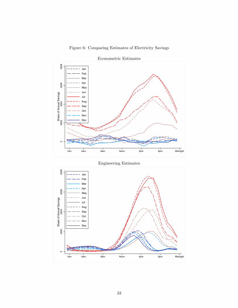
Figure 6: Comparing Estimates of Electricity Savings

Econometric Estimates0

.000

2.0

004

.000

6.0

008

Shar

e of

Ann

ual S

avin

gs

1am 4am 8am Noon 4pm 8pm Midnight

Jan

Feb

Mar

Apr

May

Jun

Jul

Aug

Sep

Oct

Nov

Dec

Engineering Estimates

0.0

002

.000

4.0

006

.000

8Sh

are

of A

nnua

l Sav

ings

1am 4am 8am Noon 4pm 8pm Midnight

Jan

Feb

Mar

Apr

May

Jun

Jul

Aug

Sep

Oct

Nov

Dec

33

Figure 7: Savings Profiles for Selected Energy-Efficiency Investments

0.0

002

.000

4.0

006

.000

8Sh

are

of A

nnua

l Sav

ings

1am 4am 8am Noon 4pm 8pm Midnight

Jan

Feb

Mar

Apr

May

Jun

Jul

Aug

Sep

Oct

Nov

Dec

Residential Lighting

0.0

002

.000

4.0

006

.000

8Sh

are

of A

nnua

l Sav

ings

1am 4am 8am Noon 4pm 8pm Midnight

Jan

Feb

Mar

Apr

May

Jun

Jul

Aug

Sep

Oct

Nov

Dec

Residential Refrigerator or Freezer

0.0

002

.000

4.0

006

.000

8Sh

are

of A

nnua

l Sav

ings

1am 4am 8am Noon 4pm 8pm Midnight

Jan

Feb

Mar

Apr

May

Jun

Jul

Aug

Sep

Oct

Nov

Dec

Residential Clothes Washer

0.0

002

.000

4.0

006

.000

8Sh

are

of A

nnua

l Sav

ings

1am 4am 8am Noon 4pm 8pm Midnight

Jan

Feb

Mar

Apr

May

Jun

Jul

Aug

Sep

Oct

Nov

Dec

Residential Heat Pump

0.0

002

.000

4.0

006

.000

8Sh

are

of A

nnua

l Sav

ings

1am 4am 8am Noon 4pm 8pm Midnight

Jan

Feb

Mar

Apr

May

Jun

Jul

Aug

Sep

Oct

Nov

Dec

Commercial and Industrial Lighting

0.0

002

.000

4.0

006

.000

8Sh

are

of A

nnua

l Sav

ings

1am 4am 8am Noon 4pm 8pm Midnight

Jan

Feb

Mar

Apr

May

Jun

Jul

Aug

Sep

Oct

Nov

Dec

Commercial and Industrial Chillers

0.0

002

.000

4.0

006

.000

8Sh

are

of A

nnua

l Sav

ings

1am 4am 8am Noon 4pm 8pm Midnight

Jan

Feb

Mar

Apr

May

Jun

Jul

Aug

Sep

Oct

Nov

Dec

Commercial and Industrial Air Conditioning

0.0

002

.000

4.0

006

.000

8Sh

are

of A

nnua

l Sav

ings

1am 4am 8am Noon 4pm 8pm Midnight

Jan

Feb

Mar

Apr

May

Jun

Jul

Aug

Sep

Oct

Nov

Dec

Commercial and Industrial Heat Pump

Table 1: Average Energy Savings from a New Central Air Conditioner

(1) (2) (3)

Energy Savings Per Household (kWh/year) 375.3 358.0 436.3(32.2) (32.2) (36.0)

Household by hour-of-day by month-of-year fixed effects Y Y YWeek-of-sample by hour-of-day fixed effects YWeek-of-sample by hour-of-day by climate zone fixed effects Y YDrop 8 weeks pre-installation Y

Number of observations 28.6 M 28.6 M 27.3 MNumber of households 5,973 5,973 5,972

Notes: This table reports results from three separate regressions. The dependent variable in all regressionsis average hourly electricity consumption measured at the household by week-of-sample by hour-of-daylevel. The main variables of interest in these regressions are 288 month-of-year by hour-of-day indicatorsinteracted with an indicator for observations after a new air conditioner installation. Annual averageenergy savings is calculated as the weighted sum of these 288 estimates. Standard errors are clusteredby nine-digit zip code. The regressions are estimated using data from 2012 to 2015 for all participatinghouseholds.

35

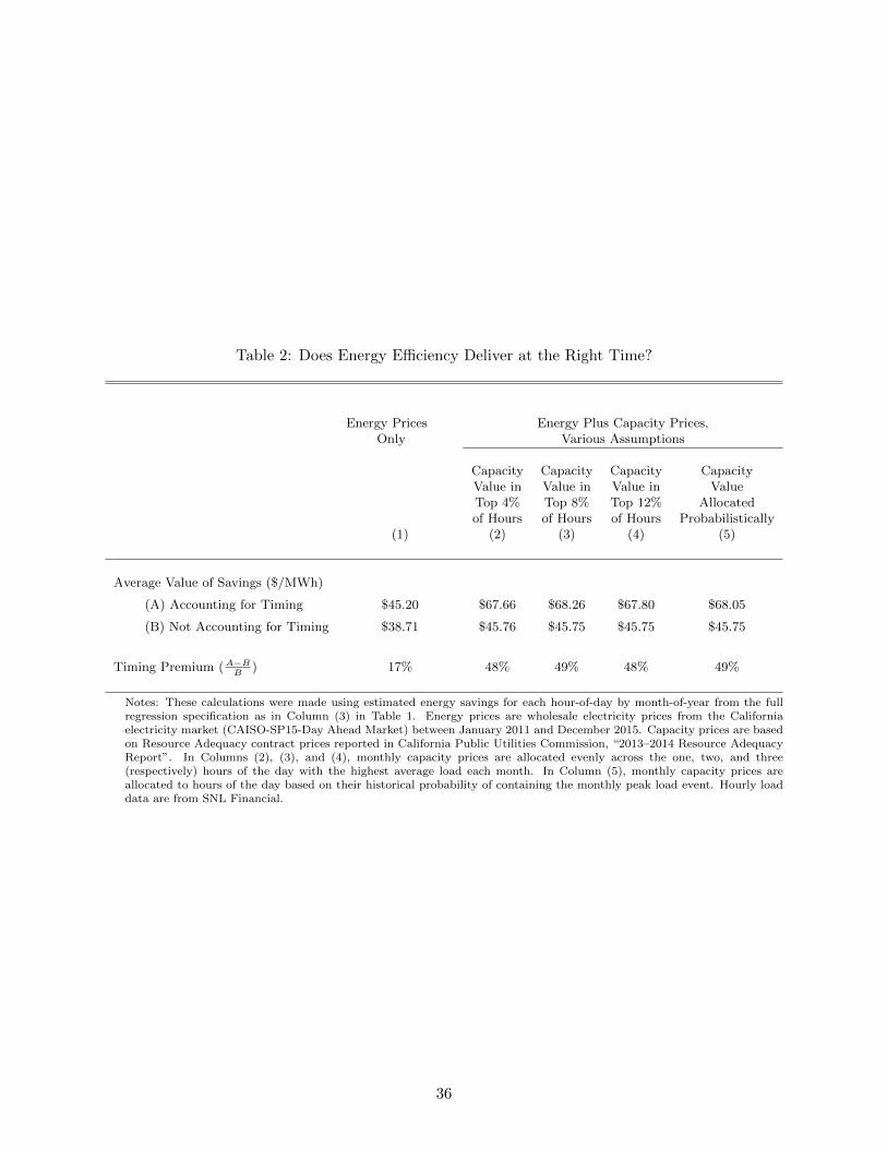
Table 2: Does Energy Efficiency Deliver at the Right Time?

Energy Prices Energy Plus Capacity Prices,Only Various Assumptions

Capacity Capacity Capacity CapacityValue in Value in Value in ValueTop 4% Top 8% Top 12% Allocatedof Hours of Hours of Hours Probabilistically

(1) (2) (3) (4) (5)

Average Value of Savings ($/MWh)

(A) Accounting for Timing $45.20 $67.66 $68.26 $67.80 $68.05

(B) Not Accounting for Timing $38.71 $45.76 $45.75 $45.75 $45.75

Timing Premium (A−BB

) 17% 48% 49% 48% 49%

Notes: These calculations were made using estimated energy savings for each hour-of-day by month-of-year from the fullregression specification as in Column (3) in Table 1. Energy prices are wholesale electricity prices from the Californiaelectricity market (CAISO-SP15-Day Ahead Market) between January 2011 and December 2015. Capacity prices are basedon Resource Adequacy contract prices reported in California Public Utilities Commission, “2013–2014 Resource AdequacyReport”. In Columns (2), (3), and (4), monthly capacity prices are allocated evenly across the one, two, and three(respectively) hours of the day with the highest average load each month. In Column (5), monthly capacity prices areallocated to hours of the day based on their historical probability of containing the monthly peak load event. Hourly loaddata are from SNL Financial.

36

Table 3: Timing Premiums for Selected Energy-Efficiency Investments

Mid- New NewCalifornia Texas Atlantic Midwest York England Average(CAISO) (ERCOT) (PJM) (MISO) (NYISO) (ISONE)

A. Residential

Air Conditioning 48% 54% 30% 21% 11% 9% 29%(Econometric Estimates)

Air Conditioning 64% 69% 33% 25% 26% 18% 39%

Lighting 12% 7% 7% 5% 9% 8% 8%

Clothes Washers 10% 14% 13% 13% 14% 13% 13%

Refrigerator or Freezer 7% 7% 3% 3% 3% 2% 4%

Heat Pump 6% 10% 4% 0% 3% 5% 5%

B. Commercial and Industrial

Heat Pump 38% 47% 27% 23% 23% 16% 29%

Chillers 34% 41% 23% 21% 18% 11% 25%

Air Conditioners 32% 39% 23% 21% 20% 13% 25%

Lighting 11% 13% 10% 9% 10% 8% 10%

Notes: This table reports the estimated timing premiums for nine energy efficiency investments. As in the final rowof Table 2, the statistics in each cell of this table represent the additional value (in percentage terms) compared to aninvestment with a completely flat savings profile. Except for the first row (econometric estimates for air conditioning), allestimates are based on engineering estimates of savings profiles from the California Public Utility Commission’s Databasefor Energy Efficient Resources. Values are estimated using wholesale energy prices and capacity prices from six majorU.S. markets as indicated in row headings. See text for details. The final column is the simple average across markets.

37

Not For Publication Appendix

A Electricity Market Data

A.1 Wholesale Electricity Prices and Load

Hourly wholesale price data are day-ahead prices from SNL Financial and are for 2011–2015. For

California, we use CAISO market at the SP-15 node. For New England, we use ISO-NE real-time

prices at the H Internal hub. For Texas, we use ERCOT real-time prices at the HB North hub. For

New York, we use NYISO real-time prices at the J Hub. For PJM, we use prices at the Western hub.

For MISO, we use prices at the Illinois hub. All times in the paper are reported in local prevailing time:

Standard Time or Daylight Time according to which is in effect. The load data in each market come

from the SNL hourly “Actual Load” series for 2011–2015. Appendix Figure 1 plots hourly average

load profiles by month-of-year for each market.

A.2 Capacity Prices

Capacity values were calculated for each electricity market under a range of assumptions. For each

market, we used auction or regulatory data to infer monthly or annual capacity prices, and allocated

those values across hours based on historical hourly load. Capacity market institutions vary across

regions, so capacity values are not perfectly comparable across markets. However, we have attempted

to use relatively comparable data and methods and to be transparent about our exact sources and

calculations.

A.2.1 California (CAISO)

There is no capacity auction in CAISO, but the California Public Utilities Commission (CPUC)

surveys utilities to track bilateral capacity contract prices. We use monthly capacity contract prices

from the CPUC “2013–2014 Resource Adequacy Report,” page 28, Table 13. This document reports

average, 85th-percentile, and maximum contract prices for each month. We use the 85th-percentile

values, on the reasoning that these provide a conservative estimate of the marginal cost of procuring

capacity (We could instead use the maximum, but choose the 85th percentile to limit the influence of

potential outlier observations). These reported prices include capacity contracts from 2013 through

2017. However, most of the reported transactions are for 2013–2015 (page 29, Figure 9).

A.2.2 New York (NYISO)

Capacity prices for New York come from NYISO’s monthly spot capacity auctions for the NYCA

region from May 2013 through April 2016. This auction runs two to four days prior to the beginning

of the month being transacted for. NYISO also runs auctions for six-month “strips” of summer or

winter capacity, as well as additional monthly auctions one to five months in advance.

1

Not For Publication Appendix

A.2.3 New England (ISO-NE)

Capacity prices for New England come from ISO-NE’s annual “forward capacity auctions” for 2013

through 2016, as reported by SNL Financial. We use the simple average of prices across the several

zones in the market.

A.2.4 Mid-Atlantic (PJM)

Capacity prices for PJM are “Market Clearing Prices” from the annual “Base Residual Auction.”

We use the simple average across years and geographic zones for 2013–2016. Data are from SNL

Financial.

A.2.5 Midwest (MISO)

Capacity prices for MISO come from annual capacity auction prices for 2013 through 2016. We use

the simple average of prices across the several geographic zones. Data are from SNL Financial.

2

Not For Publication Appendix

Appendix Figure 1: Load Profiles in Six Major U.S. Electricity Markets

(a) California (CAISO)

20,0

0025

,000

30,0

0035

,000

40,0

00Av

erag

e H

ourly

Loa

d (M

W)

1am 4am 8am Noon 4pm 8pm Midnight

Jan

Feb

Mar

Apr

May

Jun

Jul

Aug

Sep

Oct

Nov

Dec

(b) Texas (ERCOT)

30,0

0040

,000

50,0

0060

,000

Aver

age

Hou

rly L

oad

(MW

)1am 4am 8am Noon 4pm 8pm Midnight

Jan

Feb

Mar

Apr

May

Jun

Jul

Aug

Sep

Oct

Nov

Dec

(c) Mid-Atlantic (PJM)

60,0

0080

,000

100,

000

120,

000

140,

000

Aver

age

Hou

rly L

oad

(MW

)

1am 4am 8am Noon 4pm 8pm Midnight

Jan

Feb

Mar

Apr

May

Jun

Jul

Aug

Sep

Oct

Nov

Dec

(d) Midwest (MISO)50

,000

60,0

0070

,000

80,0

0090

,000

Aver

age

Hou

rly L

oad

(MW

)

1am 4am 8am Noon 4pm 8pm Midnight

Jan

Feb

Mar

Apr

May

Jun

Jul

Aug

Sep

Oct

Nov

Dec

(e) New York (NYISO)

10,0

0015

,000

20,0

0025

,000

Aver

age

Hou

rly L

oad

(MW

)

1am 4am 8am Noon 4pm 8pm Midnight

Jan

Feb

Mar

Apr

May

Jun

Jul

Aug

Sep

Oct

Nov

Dec

(f) New England (ISONE)

10,0

0012

,000

14,0

0016

,000

18,0

0020

,000

Aver

age

Hou

rly L

oad

(MW

)

1am 4am 8am Noon 4pm 8pm Midnight

Jan

Feb

Mar

Apr

May

Jun

Jul

Aug

Sep

Oct

Nov

Dec

3

Not For Publication Appendix

B Additional Data Description

B.1 Program Data

The program data describe all 10,848 households who participated in the Quality Installation Program

program between 2010 and 2015. These data were provided by Southern California Edison. We

drop 968 duplicate participant records. These records have the exact same account number as other

participant records, so are clear duplicates. We also drop an additional 291 households who installed a

new heat pump rather than a new central air conditioner; the expected energy savings for heat pumps

follows a very different temporal pattern than the temporal pattern for air conditioning so it does not

make sense to include these participants. We further drop 2,431 households who participated before

the start of 2012; we use electricity consumption data beginning in 2012, so these early participants

would not contribute to our savings estimates. We also drop an additional 757 households who installed

rooftop solar at any time during our sample period; rooftop solar dramatically changes household net

electricity consumption (we only observe net consumption, not generation and consumption separately)

so we drop these households to avoid biasing our savings estimates. In addition, we drop 60 households

for whom we do not have a nine-digit zip code; a nine-digit zip code is required for merging with

temperature data, and we cluster all standard errors at the nine-digit zip code. We successfully

merged 94% of the participant records to the electricity consumption data, so we are left with a total

of 5,973 participants in our analysis dataset. Appendix Figure 2 shows the pattern of participation

between 2012 and 2015.

B.2 Electricity Consumption Data

The electricity consumption data describe hourly electricity consumption for all program participants.

We were provided with the complete history of hourly consumption for these households beginning

when each household received a smart meter and continuing until August 2015, or, in some cases,

somewhat before August 2015. Most Southern California Edison customers received a smart meter

for the first time in either 2011 or 2012. Appendix Figure 3 shows the number of participants with

smart meter billing data during each week of the sample.

B.3 Engineering-Based Savings Profiles

Appendix Figure 4 plots savings profiles for eight additional energy-efficiency investments. These fig-

ures are constructed in exactly the same way as Figure 7, and describe five residential investments and

three commercial/industrial investments. As described in the paper, these engineering-based savings

profiles come from the Database for Energy Efficient Resources (DEER), maintained by the California

Public Utilities Commission. We use values developed in 2013/2014 for DEER 2011, reported in the

file DEER2011-HrlyProfiles-SCE.xls. For each energy-efficiency investment the DEER reports 8,760

numbers, one for each hour of the year. We use these data to construct average hourly profiles by

4

Not For Publication Appendix

month. These savings profiles are intended to reflect average impacts in Southern California Edison

territory.

The underlying model that generates the DEER hourly profiles does not account for daylight savings

time. Building occupants are assumed to observe Standard Time for the full year. As a result, the

model inputs for physical phenomena such as solar angle and temperature are correct, but inputs

related to human schedules, like building opening times, are “off” by one hour. Some analysts adjust

for daylight savings after the fact by “shifting” the DEER profile one hour: that is, replacing predicted

savings for all hours during Daylight Time with predicted savings one hour later. This corrects building

schedules but introduces error in physical factors. Whether such a shift helps or hurts accuracy depends

on whether building schedules or physical factors are more important in determining hourly savings.

We do not make any adjustments to the DEER profiles in our main specifications. If we do impose

a “shift” during Daylight Time, the estimated timing premiums for DEER investments change only

slightly.

5

Not For Publication Appendix

Appendix Figure 2: Histogram of Installation Dates

010

020

030

040

050

0In

stal

latio

ns

Jan 2012 Jan 2013 Jan 2014 Jan 2015Month

6

Not For Publication Appendix

Appendix Figure 3: Number of Participants with Smart Meter Data

01,

000

2,00

03,

000

4,00

05,

000

6,00

0N

umbe

r of

Met

ers

1/1/

2012

7/1/

2012

1/1/

2013

7/1/

2013

1/1/

2014

7/1/

2014

1/1/

2015

7/1/

2015

7

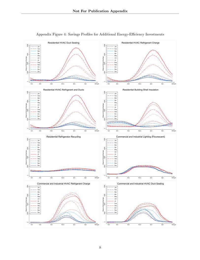
Not For Publication Appendix

Appendix Figure 4: Savings Profiles for Additional Energy-Efficiency Investments

0.0

002

.000

4.0

006

.000

8Sh

are

of A

nnua

l Sav

ings

1am 4am 8am Noon 4pm 8pm Midnight

Jan

Feb

Mar

Apr

May

Jun

Jul

Aug

Sep

Oct

Nov

Dec

Residential HVAC Duct Sealing

0.0

002

.000

4.0

006

.000

8Sh

are

of A

nnua

l Sav

ings

1am 4am 8am Noon 4pm 8pm Midnight

Jan

Feb

Mar

Apr

May

Jun

Jul

Aug

Sep

Oct

Nov

Dec

Residential HVAC Refrigerant Charge

0.0

002

.000

4.0

006

.000

8Sh

are

of A

nnua

l Sav

ings

1am 4am 8am Noon 4pm 8pm Midnight

Jan

Feb

Mar

Apr

May

Jun

Jul

Aug

Sep

Oct

Nov

Dec

Residential HVAC Refrigerant and Ducts

0.0

002

.000

4.0

006

.000

8Sh

are

of A

nnua

l Sav

ings

1am 4am 8am Noon 4pm 8pm Midnight

Jan

Feb

Mar

Apr

May

Jun

Jul

Aug

Sep

Oct

Nov

Dec

Residential Building Shell Insulation

0.0

002

.000

4.0

006

.000

8Sh

are

of A

nnua

l Sav

ings

1am 4am 8am Noon 4pm 8pm Midnight

Jan

Feb

Mar

Apr

May

Jun

Jul

Aug

Sep

Oct

Nov

Dec

Residential Refrigerator Recycling

0.0

002

.000

4.0

006

.000

8Sh

are

of A

nnua

l Sav

ings

1am 4am 8am Noon 4pm 8pm Midnight

Jan

Feb

Mar

Apr

May

Jun

Jul

Aug

Sep

Oct

Nov

Dec

Commercial and Industrial Lighting (Flourescent)

0.0

002

.000

4.0

006

.000

8Sh

are

of A

nnua

l Sav

ings

1am 4am 8am Noon 4pm 8pm Midnight

Jan

Feb

Mar

Apr

May

Jun

Jul

Aug

Sep

Oct

Nov

Dec

Commercial and Industrial HVAC Refrigerant Charge

0.0

002

.000

4.0

006

.000

8Sh

are

of A

nnua

l Sav

ings

1am 4am 8am Noon 4pm 8pm Midnight

Jan

Feb

Mar

Apr

May

Jun

Jul

Aug

Sep

Oct

Nov

Dec

Commercial and Industrial HVAC Duct Sealing

8

Not For Publication Appendix

C Alternative Specifications Using Data from Non-Participants

This section presents estimates from alternative specifications which incorporate electricity consump-

tion data from non-participating households. Overall, these alternative estimates are quite similar to

the main estimates in the paper.

The key challenge in our empirical analysis is to construct a counterfactual for how much electricity the

participants would have consumed had they not installed a new air conditioner. The analyses in the

paper construct this counterfactual using data from participants only, exploiting the natural variation

in the timing of program participation to control for trends in electricity consumption, weather, and

other time-varying factors. An alternative approach, however, is to estimate the model using data

from both participants and non-participants.

There are advantages and disadvantages with this alternative approach. The potential advantage of

including non-participant data is that these data may help better control for trends in electricity

consumption, weather, and other time effects, while also potentially improving the precision of the

estimates. The disadvantage is that non-participants tend to be quite different from participants,

making them potentially a less valid counterfactual. Without any ex ante reason to prefer one approach

over the other, it makes sense to report estimates from both approaches.

Appendix Table 1 provides descriptive statistics. The columns refer to three different samples. The

first column describes the 5,973 participants used for the main estimates in the paper. The second col-

umn describes a random sample of non-participants. We were provided with data from a 5% random

sample of Southern California Edison residential customers who did not participate in the program,

and this is a random subset of 5,973 households from that sample. Finally, the third column describes

a matched sample of non-participants. For the matched sample we selected non-participants based on

zip codes. In particular, for each participant, we randomly selected a non-participant from the same

nine-digit zip code, or five-digit zip code when nine-digit zip code is not available. Weather is a major

determinant of electricity consumption so this matching ensures that comparison households are experi-

encing approximately the same weather as the treatment households. In addition, households in close

geographic proximity tend to have similar income and other demographics. Some non-participants

matched to more than one participant, yielding 5,633 unique households in the matched sample of

non-participants. For both random and matched samples we excluded households with rooftop solar

or a missing nine-digit zip code, just as we did for participants.

Across all households, mean hourly electricity consumption is about one kWh per hour. Participants

tend to consume more than non-participants, especially during summer months. But this appears to

be largely a question of geography and the pattern of consumption in the matched sample is much

more similar to participants. More generally, the characteristics of the matched sample are more

similar but not identical to the characteristics of participants. Among participants, 13% are on the

low-income tariff, compared to 30% in the random sample and 25% in the matched sample. Similarly,

only 2% of participants are on the all-electric tariff, compared to 10% in the random sample and 6.5%

9

Not For Publication Appendix

in the matched sample.

We used these alternative samples to construct alternative estimates of several of our main results.

Appendix Figure 5 plots event study estimates analogous to Figure 1 in the paper. Whereas the event

study figure in the paper is estimated using data from participants only, these are estimated using

data from both participants and non-participants. The plots on the top include the random sample of

non-participants while the plots on the bottom include the matched sample. These alternative event

studies follow a very similar pattern to the event study figures in the paper. Summer consumption

drops sharply in the year that the new air conditioners are installed and the magnitude of this decrease

is 0.2 kilowatt hours per hour, identical to the decrease in the event study figure in the paper. Moreover,

the pattern for winter is very similar to the event study figure in the paper, with no change when the

new air conditioners are installed.

Next, Appendix Table 2 reports regression estimates of total energy savings from new air conditioner

installation. This table is constructed in exactly the same way as Table 1, but estimated using data

from both participants and non-participants. Including data from non-participants has little overall

effect. The estimates are slightly larger, but the pattern across specifications is similar, increasing

when dropping eight weeks pre-installation in Column (3).

Finally, Appendix Figure 6 plots estimates of energy savings by month-of-year and hour-of-day. These

figures are constructed in exactly the same way as Figure 6, but are estimated using data from both

participants and non-participants. Overall, including data from non-participants has very little effect

on the temporal pattern of savings. Electricity savings still tend to occur disproportionately during

July and August, and during the hours 3 p.m. to 9 p.m. In addition, during winter months the

estimates remain very close to zero during all hours of the day. Moreover, the random and matched

samples yield virtually identical estimates across hours and months.

10

Not For Publication Appendix

Appendix Figure 5: Event Study Figures, Alternative Specifications

Random Sample of Non-Participants

Summer Winter

-.3

-.2

-.1

0.1

.2H

ourly

Ele

tric

ity C

onsu

mpt

ion

(KW

h)

-3 -2 -1 0 1 2 3Years Before and After Replacement

-.3

-.2

-.1

0.1

.2H

ourly

Ele

tric

ity C

onsu

mpt

ion

(KW

h)

-3 -2 -1 0 1 2 3Years Before and After Replacement

Matched Sample of Non-Participants

Summer Winter

-.3

-.2

-.1

0.1

.2H

ourly

Ele

tric

ity C

onsu

mpt

ion

(KW

h)

-3 -2 -1 0 1 2 3Years Before and After Replacement

-.3

-.2

-.1

0.1

.2H

ourly

Ele

tric

ity C

onsu

mpt

ion

(KW

h)

-3 -2 -1 0 1 2 3Years Before and After Replacement

11

Not For Publication Appendix

Appendix Figure 6: Econometric Estimates of Electricity Savings, Alternative Specifications

Random Sample of Non-Participants

0.0

002

.000

4.0

006

.000

8Sh

are

of A

nnua

l Sav

ings

1am 4am 8am Noon 4pm 8pm Midnight

Jan

Feb

Mar

Apr

May

Jun

Jul

Aug

Sep

Oct

Nov

Dec

Matched Sample of Non-Participants

0.0

002

.000

4.0

006

.000

8Sh

are

of A

nnua

l Sav

ings

1am 4am 8am Noon 4pm 8pm Midnight

Jan

Feb

Mar

Apr

May

Jun

Jul

Aug

Sep

Oct

Nov

Dec

Not For Publication Appendix

Appendix Table 1: Smart Meter Data, Descriptive Statistics

Random Matched p-Value: p-Value:Participants Sample of Sample of Column 1 vs Column 1 vs

Non-Participants Non-Participants Column 2 Column 3(1) (2) (3) (4) (5)

Mean Hourly Electricity ConsumptionAll Months 1.076 0.878 1.025 0.000 0.000Summer Months (July and August) 1.521 1.205 1.480 0.000 0.000Winter Months (January and February) 0.852 0.729 0.806 0.000 0.000

Type of Electricity TariffProportion on Low-Income Tariff 0.128 0.303 0.254 0.000 0.000Proportion on All-Electric Tariff 0.020 0.101 0.065 0.000 0.000

Notes: Columns (1), (2), and (3) report the variables listed in the row headings for the group listed at the top of the column.There are a total of 5,973 participants and an equal number of non-participating households in the random and matched samples.Electricity consumption is measured in kilowatt hours. Columns (4) and (5) report p-values from tests that the means in thesubsamples are equal.

Not For Publication Appendix

Appendix Table 2: Average Energy Savings, Alternative Specifications

(1) (2) (3)

Random Sample of Non-Participants

Energy Savings Per Household (kWh/year) 494.4 435.8 507.3(42.8) (42.6) (47.5)

Number of observations 27.0 M 27.0 M 26.4 MNumber of households 5,976 5,976 5,975

Matched Sample of Non-Participants

Energy Savings Per Household (kWh/year) 447.9 434.5 503.4(43.3) (42.8) (47.3)

Number of observations 27.2 M 27.2 M 26.6 MNumber of households 5,893 5,893 5,892

Household by hour-of-day by month-of-year fixed effects Y Y YWeek-of-sample by hour-of-day fixed effects YWeek-of-sample by hour-of-day by climate zone fixed effects Y YDrop 8 weeks pre-installation Y

Notes: This table reports results from six separate regressions and is identical to Table 1 in the paperexcept for the sample includes data on non-participating households. In particular, Panel A includes a ran-dom sample of non-participating households and Panel B includes a matched sample of non-participatinghouseholds in which the non-participating households are drawn from the same nine digit zip code as par-ticipating households. For computational reasons, we restrict these regressions to a 50% random sampleof participating households along with an equal number of non-participating households.