DO EPA REGULATIONS AFFECT LABOR DEMAND? EVIDENCE FROM THE PULP AND PAPER INDUSTRY

by

Wayne B. Gray Clark University and NBER

Ronald J. Shadbegian National Center for Environmental Economics

Chunbei Wang University of Massachusetts - Dartmouth

Merve Cebi University of Massachusetts - Dartmouth

CES 13-39 August, 2013

The research program of the Center for Economic Studies (CES) produces a wide range of economic analyses to improve the statistical programs of the U.S. Census Bureau. Many of these analyses take the form of CES research papers. The papers have not undergone the review accorded Census Bureau publications and no endorsement should be inferred. Any opinions and conclusions expressed herein are those of the author(s) and do not necessarily represent the views of the U.S. Census Bureau. All results have been reviewed to ensure that no confidential information is disclosed. Republication in whole or part must be cleared with the authors. To obtain information about the series, see www.census.gov/ces or contact Fariha Kamal, Editor, Discussion Papers, U.S. Census Bureau, Center for Economic Studies 2K132B, 4600 Silver Hill Road, Washington, DC 20233, CES.Papers.List@census.gov.

Abstract

The popular belief is that environmental regulation must reduce employment, since such regulations are expected to increase production costs, which would raise prices and thus reduce demand for output, at least in a competitive market. Although this effect might seem obvious, a careful microeconomic analysis shows that it is not guaranteed. Even if environmental regulation reduces output in the regulated industry, abating pollution could require additional labor (e.g. to monitor the abatement capital and meet EPA reporting requirements). It is also possible for pollution abatement technologies to be labor enhancing. In this paper we analyze how a particular EPA regulation, the so-called “Cluster Rule” (CR) imposed on the pulp and paper industry in 2001, affected employment in that sector. Using establishment level data from the Census of Manufacturers and Annual Survey of Manufacturers at the U.S. Census Bureau from 1992-2007 we find evidence of small employment declines (on the order of 3%-7%), which are sometimes statistically significant, at a subset of the plants covered by the CR. i

Any opinions and conclusions expressed herein are those of the author(s) and do not necessarily represent the views of the U.S. Census Bureau or the U.S. Environmental Protection Agency. All results have been reviewed to ensure that no confidential information is disclosed. We thank Wang Jin and Shital Sharma for excellent research assistance; we also thank Jim Davis at the Boston Research Data Center for his continued help, and Reed Walker and participants at the 2011 AERE Summer Conference and the Environmental Economics seminar at Harvard University’s Kennedy School for helpful comments. Any remaining errors are ours.

3

1. INTRODUCTION

Prior to 1970 environmental regulation was done principally by state and local agencies –

for the most part with little enforcement activity. After the establishment of the Environmental

Protection Agency (EPA) in the early 1970s, and the passage of the Clean Air and Clean Water

Acts, the federal government took over the primary role in regulating environmental quality,

imposing much stricter regulations with correspondingly stricter enforcement. Since the

establishment of EPA the federal government has continually required U.S. manufacturing plants

to further reduce their emission levels. Even though the stringency of environmental regulation

has continually increased, U.S. manufacturing plants have only faced a moderate increase in their

level of spending on pollution abatement – pollution abatement costs increased from roughly 0.3

percent of total manufacturing shipments in 1973 to only 0.4 percent in 2005. On the other hand,

certain highly polluting, highly regulated industries face higher abatement costs – pulp and

paper, steel, and oil refining each spend approximately 1% of their shipments to comply with

environmental regulations in 2005 (PACE 20051).

Although pollution abatement expenditures are a very small fraction of the manufacturing

sectors’ operating costs (even for the most highly regulated industries) the popular belief is that

environmental regulation must reduce employment. The standard explanation for this effect is

that such regulations increase production costs, which would raise prices and reduce demand for

output, thus reducing employment (at least in a competitive market). Stricter regulations may

encourage plants to adopt more efficient production technologies that are capital-intensive and

thus reduce employment. Although this effect might seem obvious, a careful microeconomic

analysis shows that it is not guaranteed. Even if environmental regulation reduces output in the

1 “Pollution Abatement Costs and Expenditures: 2005” (MA200-2005) U.S. Dept of Commerce, Bureau of the Census, April 2008.

4

regulated industry, abating pollution could require additional labor (e.g. to monitor the abatement

capital and meet EPA reporting requirements). It is also possible for pollution abatement

technologies to be labor enhancing [see Berman and Bui (2001a) and Morgenstern et al (2002)].

Given current high unemployment rates, it is natural for policy-makers to be concerned that new,

more stringent environmental regulations will lead to job loss, and hence important to test

whether these concerns are well-founded.

In this paper we analyze how a particular EPA regulation, the so-called “Cluster Rule”

(CR) imposed on the pulp and paper industry in 2001, affected employment in that sector. The

CR was the first integrated, multi-media regulation imposed on a single industry. The goal of the

CR was to reduce the pulp and paper industry’s toxic releases into the air and water, driven in

part by concerns about trace amounts of dioxin being formed at mills that used chlorine

bleaching in combination with the kraft chemical pulping technology. The stringency of the CR

varied across plants, with larger air polluters subject to MACT (maximum achievable control

technology) technology standards, and chemical pulping mills subject to BAT (best available

technology) technology standards for their water pollution discharges. By promulgating both air

and water regulations at the same time EPA made it possible for pulp and paper mills to select

the best combination of pollution prevention and control technologies, with the hope of reducing

the regulatory burden. By imposing different requirements on plants within the same industry,

the CR allows us to identify the size of that regulatory burden, specifically the impact (if any)

that the CR had on employment at the affected plants.

Much of the existing literature relies on variations in environmental regulation across

geographical areas or across industries to identify its effect on employment. In contrast, we are

the first to use establishment level panel data within a single industry to rigorously examine the

5

net employment effects of a specific regulation, the CR, on the directly regulated sector.2 By

identifying which plants are subject to the CR and when, we can construct accurate control

groups, which allows us to estimate the effect of regulation on employment with more precision

using difference-in-differences models. Second, the existing literature tends to measure the

stringency of environmental regulation either with broad measures of all environmental

regulations (e.g. total pollution abatement costs) or with measures targeting a single

environmental medium (e.g. county non-attainment with specific National Ambient Air Quality

Standards ). In contrast, the CR is a uniquely multi-media regulation, whose employment effects

may have important implications for future policy-making.

Using establishment level data from the Census of Manufacturers and Annual Survey of

Manufacturers at the U.S. Census Bureau from 1992-2007, we find some evidence of small

employment declines (on the order of 3%-7%) associated with the adoption of the CR, which are

sometimes statistically significant. These declines are concentrated in plants covered by the

BAT water pollution standards; employment effects at plants covered by only the MACT air

rules are more often positive than negative, though generally insignificant.

Section 2 provides background information on pollution from the pulp and paper industry

and a brief history of the Cluster Rule. Section 3 reviews the relevant literature. Section 4

outlines a theoretical framework of the impact of regulation on employment. Section 5 discusses

the data and empirical methodology. Section 6 presents the results, followed by concluding

2 Environmental regulations may also produce jobs in other industries outside the directly regulated sector, e.g. in the environmental protection. Thus to calculate the net employment effect of any regulation for the entire economy requires estimating both the job gains as well as the job losses, if any, due to the imposition of that regulation. This exercise is beyond the scope of this paper, but we expect that in a full-employment economy that the number of jobs created by new pollution abatement spending would approximately equal the number of jobs lost in the regulated sector as resources are reallocated towards the environmental protection sector.

6

comments in section 7.

2. REGULATING THE PULP AND PAPER INDUSTRY

Over the past 40 years the U.S. manufacturing sector has faced increasingly stringent

environmental regulations with stricter enforcement and monitoring. The increasing stringency

of environmental regulation has caused traditional ‘smokestack’ industries, like the pulp and

paper industry, to devote more resources to pollution abatement. However, even though the pulp

and paper industry is one of the most highly regulated industries, due to the inherent polluting

nature of the production process, and spends a relatively large amount of resources on pollution

abatement, it has historically spent less than 2% of its overall costs on pollution abatement.

The entire pulp and paper industry faces substantial levels of environmental regulation,

however, plants in this industry are differentially affected by regulation, depending in part on

their technology (pulp and integrated mills vs. non-integrated mills3), age, location, and the level

of regulatory effort directed at the plant. Previous research, including Gray and Shadbegian

(2003), has found that the main factor determining the extent of the regulatory impact on a plant

is whether or not the plant contains a pulping facility, since the pulping process (separating the

fibers need to make paper from raw wood) is much more pollution intensive than the paper-

making process.4 Furthermore, different pulping processes generate different types of pollution:

mechanical pulping is more energy intensive, producing air pollution from a power boiler, while

chemical pulping could produce water pollution from spent chemicals, at least some of them

potentially toxic. Moreover, to produce white paper the pulp must be bleached. The Kraft

3 Integrated mills produce their own pulp and non-integrated mills purchase pulp or use recycled wastepaper. 4 The two main environmental concerns during paper-making stage are air pollution if the mill has its own power plant and the residual water pollution generated during the drying process.

7

chemical pulping process initially considered to be relatively low-polluting in terms of

conventional air and water pollution turned out to have other environmental concerns. In

particular, when combined with elemental chlorine bleaching, the Kraft pulping process creates

chloroform, furan, and trace amounts of dioxin (all potential carcinogens), raising concerns over

toxic releases that contributed, at least indirectly, to the promulgation of the Cluster Rule.

A flood in Times Beach, Missouri (located near St. Louis) helped raise public awareness

regarding the concerns about toxic pollutants in general, and in particular dioxin. On December

5th, 1982 the Meramec River flooded Times Beach, contaminating nearly the entire town with

dioxin that had been deposited by spraying to alleviate dust in the early 1970’s. The Center for

Disease Control declared that the town was uninhabitable and in 1983 the US EPA bought Times

Beach and relocated its residents, reinforcing the public perception of the dangers of dioxin.

As a result of the Times Beach incident two powerful environmental groups, the

Environmental Defense Fund and the National Wildlife Federation, sued the EPA for not

sufficiently protecting the U.S. public from the risks caused by dioxin. EPA, as part of a 1988

settlement with the environmental groups, agreed to investigate the health risks of dioxin and to

set regulations to reduce dioxin emissions. Ten years later, EPA implemented regulations that

included dioxin reductions, as part of the Cluster Rule.

The Cluster Rule

EPA initially proposed the Cluster Rule on December 17, 1993. This was the agency’s

first integrated, multi-media regulation, designed to protect human health by decreasing toxic

releases by pulp and paper mill’s into both the air and water. By simultaneously promulgating

both air and water regulations the EPA allowed pulp and paper mills to address multiple

regulatory requirements simultaneously, attempting to diminish the overall regulatory burden on

8

the mills. During the public comment period, many submissions were received from industry

representatives, governmental entities, environmental groups, and private citizens. Industry

comments asserted that EPA had underestimated the compliance costs of the proposed standards

and raised the possibility of substantial negative impacts on the industry ($20 billion in

compliance costs; 21,800 lost jobs). In response to these comments and additional data supplied

by pulp and paper industry representatives, EPA made significant changes to the proposed rule,

reducing control requirements for certain categories of plants and providing greater flexibility to

plants in choosing control options.

The final version of the rule was promulgated in 1998. To address toxic air pollutants,

EPA established maximum achievable control technology (MACT) standards (referred to as

MACT I & III) for the pulp and paper industry that required mills to abate toxic air pollutant

emissions that occurred during the pulping and bleaching stages of the manufacturing process.5

The MACT I rule regulates mills that chemically pulp wood using kraft, semi-chemical, sulfite,

or soda processes, while MACT III regulates mills that mechanically pulp wood, or pulp

secondary fiber or non-wood fibers, or produce paper or paperboard. The MACT air regulations

were expected to achieve substantial reductions in hazardous air pollutants (reduced by 59%),

sulfur (47%), volatile organic compounds (49%) and particulate matter (37%).

To address water pollution EPA also established Best Available Technology

Economically Achievable (BAT) effluent limits for toxic water pollutants created during the

bleaching process. The BAT standards were based on substituting chlorine dioxide for chlorine

in the bleaching process (i.e., using elemental chlorine-free bleaching [ECF]) or using totally

5Technology based standard to limit hazardous air pollutants, set without regard to cost.

9

chlorine-free (TCF) bleaching.6 The BAT water regulations were expected to achieve a 96%

reduction in dioxin and furan, and a 99% reduction in chloroform.

 

3. LITERATURE REVIEW: ENVIRONMENTAL REGULATION    

The question of the impact of environmental regulation on U.S. manufacturing is not a new

one. There is an extensive literature on the costs of complying with EPA regulations. Among the

studies using plant-level data, many have examined the effect of EPA regulations on productivity

[see Färe, Grosskopf and Pasurka (1986), Boyd and McClelland (1999), Berman and Bui

(2001b), and Shadbegian and Gray (2005, 2006)]. Other studies have examined how regulations

affected investment [see Gray and Shadbegian (1998)] and environmental performance [see

Magat and Viscusi (1990), Laplante and Rilstone (1996), and Shadbegian and Gray (2003,

2006)]. However, only a limited of studies have examined the impact of environmental

regulations on employment [see Berman and Bui (2001a), Greenstone (2002), Morgenstern,

Pizer and Shih (2002), Cole and Elliott (2007), Walker (2011), and Gray and Shadbegian

(2013)]. Given the high unemployment rate during the current economic crisis, and the

government’s continued efforts to reduce unemployment, policy-makers, industry, and the public

are concerned that stringent environmental regulations may reduce employment and thus

exacerbate the unemployment problem.

Berman and Bui (2001a) compiled a unique plant-level data set to estimate the impact of

air pollution regulations on labor demand in the Los Angeles, CA area – South Coast Air Quality

Management District (SCAQMD). The data set they constructed contains detailed information

on all the changes in environmental regulation including adoption date, compliance date, date of

6 Technology based standard to limit conventional and toxic discharges into water, which takes cost into consideration.

10

increase in stringency, and the regulated pollutant for all the affected manufacturing plants in the

SCAQMD. In their study Berman and Bui found that new air quality regulations introduced

between 1979 and 1992 did not in fact reduce the demand for labor in Los Angeles, but may have

actually increased it by a small amount.

Morgenstern, Pizer and Shih (2002) estimate a model (1979-1991) for four highly

polluting/regulated industries (pulp and paper, plastic, petroleum refining, and steel) to examine

the effect of higher abatement costs from regulation on employment. They conclude that

increased abatement expenditures generally do not cause a statistically significant change in

employment.

Cole and Elliot (2007) estimate a similar model to Berman and Bui (2001a) with a panel

data set on 27 industries (1999-2003) from the United Kingdom. Cole and Elliot treat their

measures of the stringency of regulation – pollution abatement operating costs as a percentage of

gross value-added and pollution abatement capital expenditures as a percentage of total capital

expenditures – both exogenously and endogenously and find, like Berman and Bui, that

environmental regulations have no statistically significant effect on employment.

Gray and Shadbegian (2013), like Cole and Elliot (2007), use a similar model to Berman

and Bui (2001a) with industry level data to analyze the impact of environmental regulation on

employment in U.S. manufacturing (1973-1994). However, Gray and Shadbegian (2013) also

examine whether or not differences in regulatory pressure across industries and over time affects

how industry employment responds to regulatory pressure. They find that more stringent

regulations (measured by pollution abatement operating costs relative to output) have a

statistically significant yet quantitatively negligible effect on employment in most cases, with a

somewhat larger effect in highly regulated industries. Gray and Shadbegian (2013) also find, as

11

expected, that regulation has a smaller impact in employment in industries in which demand is

growing faster. However, they unexpectedly find that employment is more sensitive to

regulatory pressure in industries with less competition and that the sensitivity of employment to

regulation is not significantly affected by an industry’s level of import competition.

Greenstone (2002), using a difference-in-differences model, examines the effect of

county nonattainment status for the criteria pollutants – particulate matter, sulfur dioxide, ozone

and carbon monoxide – on employment.7 Polluting plants in non-attainment areas face stricter

regulations than similar plants in attainment areas, thereby potentially raising their production

costs and lowering economic activity. Greenstone combines county attainment status information

with facility-level data from Census of Manufacturers (1972–1987) finds that nonattainment

counties (relative to attainment ones) lost roughly 590,000 jobs. Walker (2011) also finds

statistically significant employment losses in non-attainment counties (relative to counties in

attainment), with employment falling by about 15% at plants in newly designated non-attainment

areas due to new Clean Air Act regulations in the 1990s.

In sum, most past studies using plant-level data have found small or positive impacts of

stricter environmental regulation on labor demand, with the exception of Greenstone (2002) and

Walker (2011), who find more substantial reductions, looking at county non-attainment status.

However, this does not mean that there is less overall employment due to more stringent

environmental regulation, it simply suggests that the relative growth rate of employment in some

sectors differs between attainment and non-attainment areas. Now we turn to our own analysis of

employment impacts of the CR.

4. THEORETICAL FRAMEWORK 7 Greenstone also examines the effect of county non-attainment status on capital stock and output.

12

Popular wisdom holds that environmental regulation must reduce employment, because

such regulation raises the cost of production, thereby decreasing output. Nevertheless, standard

neoclassical microeconomic analysis demonstrates that this is not necessarily true. Even though it is

indeed possible for environmental regulation to result in less production, it is also possible that

pollution abatement technologies are labor enhancing. Therefore, we adopt a model derived by

Berman and Bui (2001a) that allows environmental regulation to affect labor demand via two

channels: the output elasticity of labor demand and the marginal rate of technical substitution

between labor demand and pollution abatement activity. The model developed by Berman and Bui

(2001a) was based on the partial static equilibrium model (PSEM) of Brown and Christensen

(1981). The key component of Brown and Christensen’s PSEM is that it allows the levels of

some “quasi-fixed” factors (e.g. pollution abatement investment) to be set by exogenous

constraints (e.g. environmental regulation), instead of purely by cost minimization.8 In our case,

we regard pollution abatement capital and operating costs, as well as environmental regulatory

variables as “quasi-fixed.” We treat all other “productive” factors as variable.

Assume that a perfectly competitive polluting plant minimizes costs by choosing levels of

the M variable inputs and Q “quasi-fixed” inputs. We can write the variable cost function as

follows:9

where Y is output, Pm are the prices of the variable factors, and Zn are the levels of the “quasi-fixed”

inputs. Using Shephard’s lemma produces the following set of variable input factor demands as a

8 This approach permits us to model the plant’s behavior with a variable cost function which is minimized with respect to a subset of input factors conditional on both output and the levels of the “quasi-fixed” factors. 9 Our notation is largely adopted from Berman and Bui (2001a).

),....,1,,....,1,( Zn ZPmPYFCV

13

function of output, prices, and the level of the “quasi-fixed” inputs:

The direct effect of regulation on Li is

The first term in equation (3) indicates the effect of regulation on labor demand through its effect

on output. The “output” effect of environmental regulation is typically assumed to be negative,

however Berman and Bui (2001a) note that neoclassical microeconomic theory provides no

definitive sign. For example, if plants comply with regulations by investing in abatement capital

that decreases marginal costs, dY/dR can be positive. The second term indicates the effect

regulation has on labor demand through its effect on the demand for quasi-fixed abatement

activities, Z, and the marginal rates of technical substitution between pollution abatement

activities and labor. The change in demand for pollution abatement activity caused by more

stringent regulation, dZ/dR, must be positive. The βk coefficients cannot be signed a priori, since

they depend on whether labor and pollution abatement activity are substitutes or complements.

This is the key reason why the sign of μ, the overall employment effect of regulation, cannot be

predicted from theory alone. Finally, if input factor markets are competitive and the regulated

industry makes up only a small portion of those markets, any change in regulatory stringency for

the industry will not affect the price of its inputs, thus the final term in equation (3) will drop out.

Citing data limitations, Berman and Bui (2001a) estimated the impact air pollution

regulations have on labor demand in the SCAQMD between 1979 and 1992 with the following

reduced-form version of equation (3):

j

J

j

jk

K

k

ky PZYL

11

)2(

K

k

jJ

j

jkyidR

dP

dR

dZ

dR

dYdRdL

1 1

)3(

14

Following Berman and Bui (2001a) we estimate a similar version of equation (4), augmented

with several plant characteristics as well as county and state level variables described below.10

5. DATA AND EMPIRICAL METHODOLOGY

We seek to estimate the causal effect of the CR on employment in the pulp and paper

industry. However, plants covered by the CR may be systematically different from plants not

covered by the rule, biasing a simple comparison of covered and non-covered plants. We adopt a

difference-in-differences (DiD) estimator to help control for any systematic differences between

covered and non-covered plants and any other potentially confounding factors that changed

around the time of the promulgation of the CR.

One potential concern with a DiD analysis is the possibility that the treatment and control

groups are experiencing different trends which can be misinterpreted as a different impact of the

treatment when both groups are compared with their pre-treatment values. Figures 1-3 address

this issue, showing the trends for total employment, production workers, and production worker

hours for all three groups of plants: BAT plants, MACT-only plants, and the control group.

Looking at the pre-promulgation period, we see relatively stable employment for all three

groups – if anything, there seems to be a bit of a decline in the treated groups relative to the

control group in the earlier period, which might lead the DiD analysis to overstate employment

reductions in the treatment groups.

To implement our DiD estimator we use establishment level data from the Census of 10 Cole and Elliot (2007) and Gray and Shadbegian (2013) estimate a similar model using industry level data.

RL )4(

15

Manufacturers and Annual Survey of Manufacturers at the U.S. Census Bureau from 1992-2007.

These datasets are linked together using the Longitudinal Business Database, as described in

Jarmin and Miranda (2002). Our Census data include three measures of employment: total

employment, number of production workers, and production worker hours. The data also include

the total value of shipments from the plant, materials inputs (including energy usage), and new

capital investment. We combine the Census data with data from the Lockwood Directory for

various years, identifying whether or not the plant includes a pulping process and the plant’s age.

As mentioned above, the stringency of the CR varied across plants. Out of 490 pulp and

paper mills that EPA originally estimated would be subject to the new CR MACT regulations

only 155 mills had to comply with the Air Toxics (MACT) regulations.11 Furthermore, of the

155 plants that were covered by the MACT regulations 96 of them chemically pulp wood so they

also needed to comply with the Water Toxics (BAT) standards. The remaining 335 mills did not

need to comply with either the MACT or BAT requirements of the CR. Plants needed to comply

with the MACT regulations by April 2001, while those covered by the BAT regulations had to

comply as soon as their water pollution discharge National Pollutant Discharge Elimination

System (NPDES) permit was renewed. Given that most water NPDES permits last for five

years, the effective BAT compliance dates were spread over 1998-2002. Thus we have a set of

regulations affecting multiple pollution media, with different stringency levels across plants.

This allows us multiple dimensions along which to test the impact of the Cluster Rule.

We examine whether changes in employment at plants that had to comply with the CR

before and after it became effective are similar to changes in employment at plants that did not

have to comply with the CR. Factors other than the CR also affect employment levels. The

11 EPA also separately tightened up its rules regarding hazardous air pollutants from pulp and paper mills, including those not subject to the CR, but those rules are not as stringent as the CR.

16

demand conditions in the pulp and paper industry may fluctuate over time, along with the prices

of inputs, supply of materials, and production technology, all leading to changes in employment

levels. The plants in the control group need to satisfy two conditions. First, these plants should

not be affected by the CR, which we ensure by using EPA lists of the affected plants. Second,

these plants should otherwise be very similar to the treatment group. Because plants in the

control group were in the same industry, producing similar products to the treatment group, we

expect the two groups be reasonably similar in the factors affecting their employment other than

the CR, satisfying the second condition. We limit the control group to those plants which include

some kind of pulping process, to avoid the less-comparable plants which use recycled paper or

purchase market pulp. Thus the DiD approach allows us to control for any time-invariant

unobserved heterogeneity as well as any changes over time that affect both groups similarly.

Model Specification

To obtain a raw DiD effect of the CR on plants’ employment, we can estimate the

following baseline model:

(5) lnEMPpt = 0 + 1 MACTp + 2 BATp + 3 MACTp*CR_YEARpt + 4BATp*CR_YEARpt + δt + ηs +upt

where p indexes plants and t indexes years and ηs is a vector of state dummy variables. The

dependent variable lnEMP is the log of one of our employment measures; MACT is a dummy

indicating plants that must comply with the MACT regulations of the Cluster Rule; BAT is a

dummy indicating plants that must comply with the BAT regulations of the Cluster Rule (a

proper subset of the MACT plants); and CR_YEAR is a dummy variable indicating when a plant

must begin to comply with the requirements of with the Cluster Rule. Thus MACTp*CR_YEARpt

17

and BATp*CR_YEARpt capture the change in employment at the CR-covered plants, relative to

non-covered plants, during the post-cluster rule years. The coefficients β3 and β4 thus measure

the DiD effect of the CR on employment. While β3 measures the CR effect on the MACT plants

relative to the control group, β4 measures the differential effect on the BAT plants relative to the

MACT plants, so (β3+β4) measures the CR effect on the BAT plants relative to the control group.

We use several alternative measures of employment at the plant level. First, we examine

TE, the total employment at the plant, which includes both production and non-production

workers. Although this measure has been the primary focus for researchers and policy-makers,

we might expect the impact of a regulation on employment to differ between the two groups.

Rules involving paperwork and procedural compliance might require additional non-production

workers to deal with those changes, while increases in production costs that reduced demand for

the firm’s product might have a greater impact on production worker employment. Thus, we also

considered a second employment measure - PW, the number of production workers. By

comparing the results for TE and PW, we could test for evidence of differential effects across

labor types. Finally, plants may express a change in production labor demand through changing

the hours worked instead of the number of workers. Thus we also examine a third employment

measure - PH, the production worker hours per year.

In defining the “post-CR” period, we consider both the announcement and effective dates

of the rule. The CR was announced at the end of 1997. Covered plants had to comply with

MACT regulations before April 2001, while the compliance date of BAT regulations varied over

several years, depending on when plants renewed their water discharge permit. Although we

have information on the compliance dates of each plant, we suspect that they may not be the

appropriate basis to define the post-CR period. It takes time for plants to adjust, which was why

18

the compliance date of the CR was set for years after it was announced. We expect that, as soon

as the rule was announced, plants started planning for the adjustment, including adoption of new

technology and possibly adjusting their employment levels. If the CR had an impact on

employment, the change could occur before 2001, once the announcement was made.

Supporting this concern, Gray and Shadbegian (2008) found that reductions in pollution

emissions from pulp and paper mills began before the Cluster Rule’s 2001 compliance date.

Based on these earlier results, we consider two break points, using the Cluster Rule’s 1997

announcement date as one break point (making 1998-2007 the post-CR treatment period –

CR_1998) and the 2001 enactment date as the other (making 2001-2007 the post-CR treatment

period – CR_2001)12, and estimate models using one or the other or both break points.

To isolate the effect of the CR on employment, we also need to control for plant

characteristics that are constant over time as well as other time-variant factors that might affect

employment differently between the covered and non-covered plants. As mentioned before, plant

characteristics play an important role in determining pollution levels. These characteristics may

determine whether a plant is subject to the CR and may also have a direct effect on employment

levels. For example, older plants have higher pollution levels and may be more likely to be in the

treatment group. These plants may also have different labor demand and elasticity of substitution

among factors of production and could have changed employment levels differently from non-

covered plants over time. In addition, local labor market conditions can affect a plant’s hiring

decisions, so we include a set of control variables measuring local labor market conditions: local

12 An alternative would be to find out how long it would take for plants to install the necessary equipments to comply with the CR so as to get a rough estimate of when plants might start the adjustment process. However, plants may vary in the timing of the adoption of technology. Furthermore, the timing of the adoption of technology may not be indicative of the timing of the potential employment adjustment, further complicating this approach.

19

wages, unemployment rates, and per-capita income, measured at the county level13. We also

include state fixed effects to control for any other time-invariant state-level unobserved

heterogeneities that may affect employment.14

When we include these control variables, our model can be written as:

(6) lnEMPpt = 0 + 1 MACTp + 2 BATp + 3 MACTp*CR_YEARpt + 4BATp*CR_YEARpt + ZptΓ +

ηs + δt + upt

Here Z is a set of plant characteristics, including OLD, a dummy variable indicating whether or

not the plant was started before 1960, and a set of county-level labor market conditions that

change over time, including log wage rate, log unemployment rate, and log per capita income.

One final set of analyses include plant-specific fixed effects:

(7) lnEMPpt = 0 + 3 MACTp*CR_YEARpt + 4BATp*CR_YEARpt + ZptΓ + δt + αi + upt

Including αi accounts for fixed characteristics of the plant affecting the average employment

level, but also eliminates variables (e.g. MACT, BAT, and OLD) which do not vary over time.

6. RESULTS

Baseline models

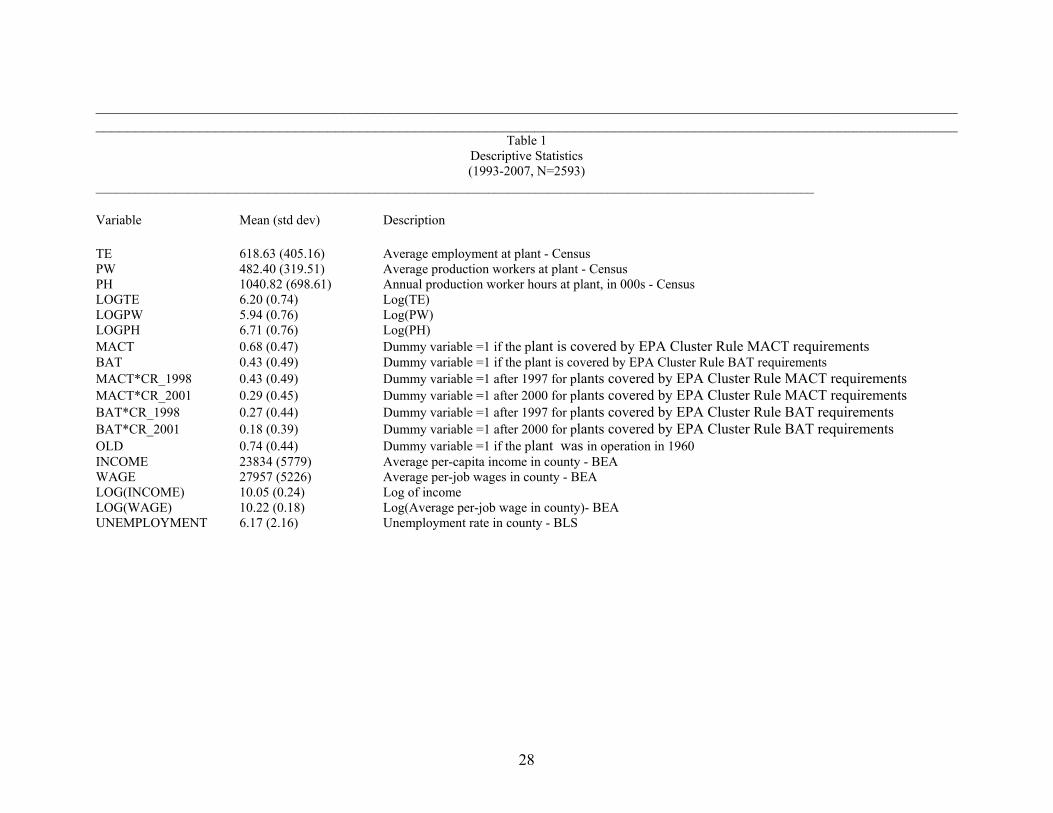
Table 1 displays the summary statistics and variable definitions. We exclude observations

with missing values for value of shipments (TVS), overall employment (TE), production worker

employment (PW), production worker hours (PH), or plants that seem to match to two different

13 Income and wage data came from the Bureau of Economic Analysis (BEA) website (http://www.bea.gov/regional/reis/), while unemployment data came from the Bureau of Labor Statistics (BLS) website (http://www.bls.gov/lau/). 14 Including these additional regressors can also increase the efficiency of our estimator.

20

Census records. None of those restrictions results in much loss of sample size. We also exclude

non-pulping plants from the analysis, about 40% of the plants in the Census data, to ensure that

the control group is as similar to the treatment group as possible (all CR plants include a pulping

process). The resulting dataset used for the analysis is an unbalanced panel, with 2,593

observations over the 1993-2007 period. About two-thirds of the observations are covered by the

MACT air requirements, while 43% are covered by the BAT water requirements. Most of the

plants (three-quarters) had been in operation since 1960, and about 60% of them include a

pulping process. The majority of employment consists of production workers, though there is

also substantial non-production employment (about one-fifth of the total).

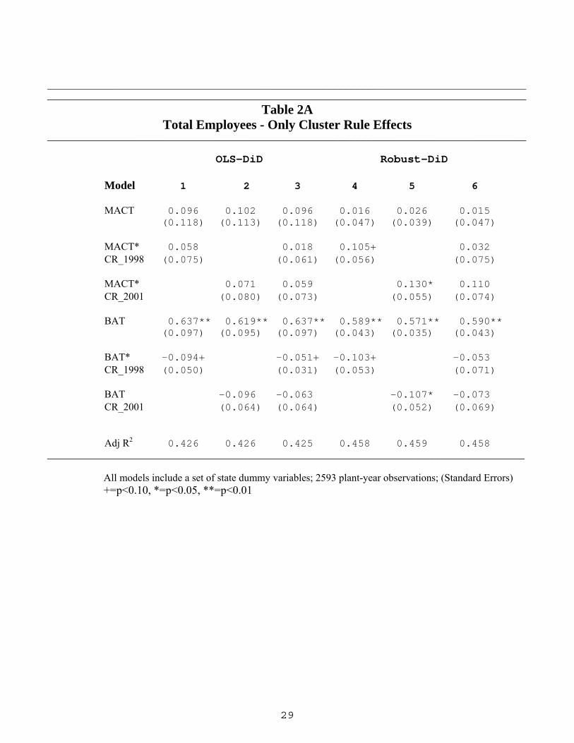
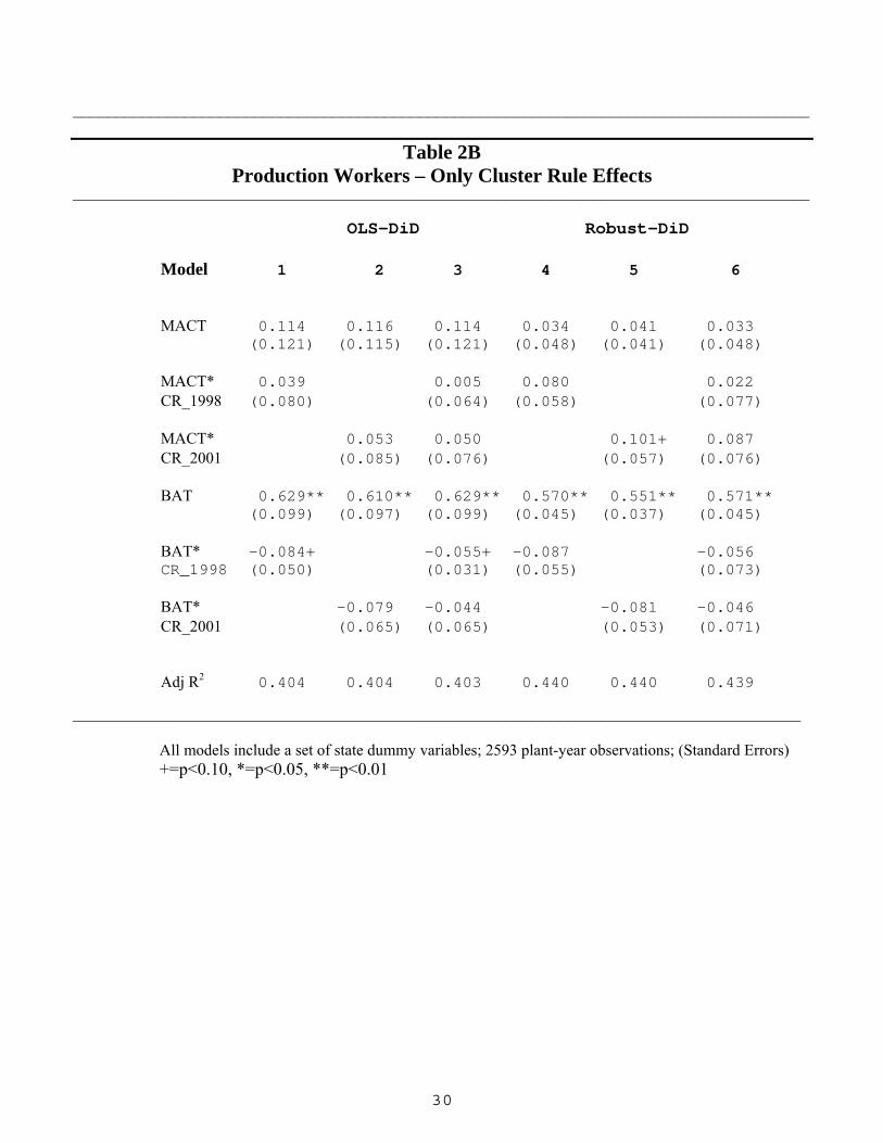
Tables 2A-2C show the results for our baseline DiD regression as described in equation

(5) for each employment measure, comparing employment effects for both BAT and MACT

plants and allowing effects to occur at the promulgation date (1998), the effective date (2001), or

both. As suggested by Bertrand et al (2004), our basic DiD results allow for correlations in errors

across years for the same plant by using standard errors that are robust to within-plant

correlations over time. Plants covered by the BAT water regulations have employment almost

two-thirds larger than plants covered only by the MACT air regulations, which are in turn about

10% larger than control plants (though the latter difference is not significant) for all three

dependent variables.

The key variables for our analysis, the DiD terms interacting the treatment categories

with promulgation or adoption date, are reasonably consistent across model specification and

employment measures, though only occasionally statistically significant. Plants covered by only

MACT air regulations tend to show positive employment changes in the post-CR period, relative

to the control group, with magnitudes on the order of 5%-10% depending on the employment

21

measure and the time period chosen. The BAT interacted dummies, on the other hand, are

consistently negative, with magnitudes on the order of 5%-10%, indicating that plants covered

by the BAT water regulations tend to have negative employment changes in the post-CR period,

relative to the MACT-only plants. Since the BAT changes relative to the control group are the

sum of these two coefficients (which are similar in magnitude, but opposite in sign) they tend to

be near zero, and are not statistically significantly different from zero.

We have some concerns with data quality, therefore we also present “RobustDiD” results

estimating an iteratively reweighted least squares model to reduce the influence of individual

data points on the coefficient estimates and correct for possibly non-normal residuals, providing

a more robust estimation.15 Focusing on the key DiD interactions, the robust BAT*CR_YEAR

coefficients are almost always close to the non-robust coefficients in sign and magnitude, while

the robust MACT*CR_YEAR coefficients tend to be larger, showing more positive impacts of

the CR on employment. Summarizing the BAT and MACT interactions from the various models,

we see that MACT-only plants have 7% to 14% higher total employment, production worker

employment, and production worker hours as compared to either the BAT plants or the control

group, with the latter two groups being relatively similar. The only statistically significant results

come from the robust DiD models. Comparing the results across years, the 2001 change seems to

be a bit larger than the 1998 ones, though not significantly so.

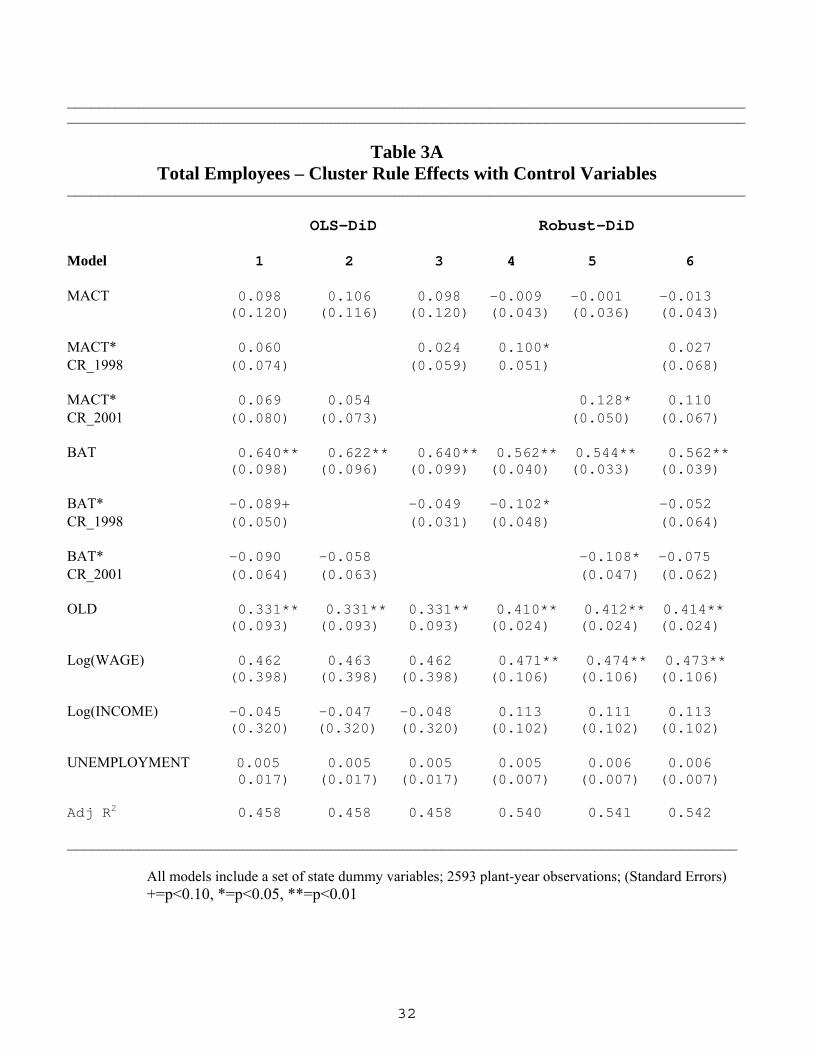
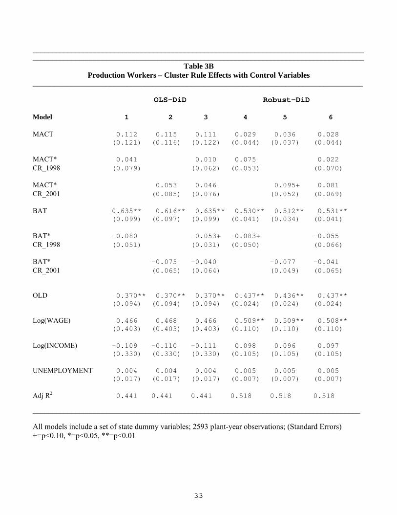
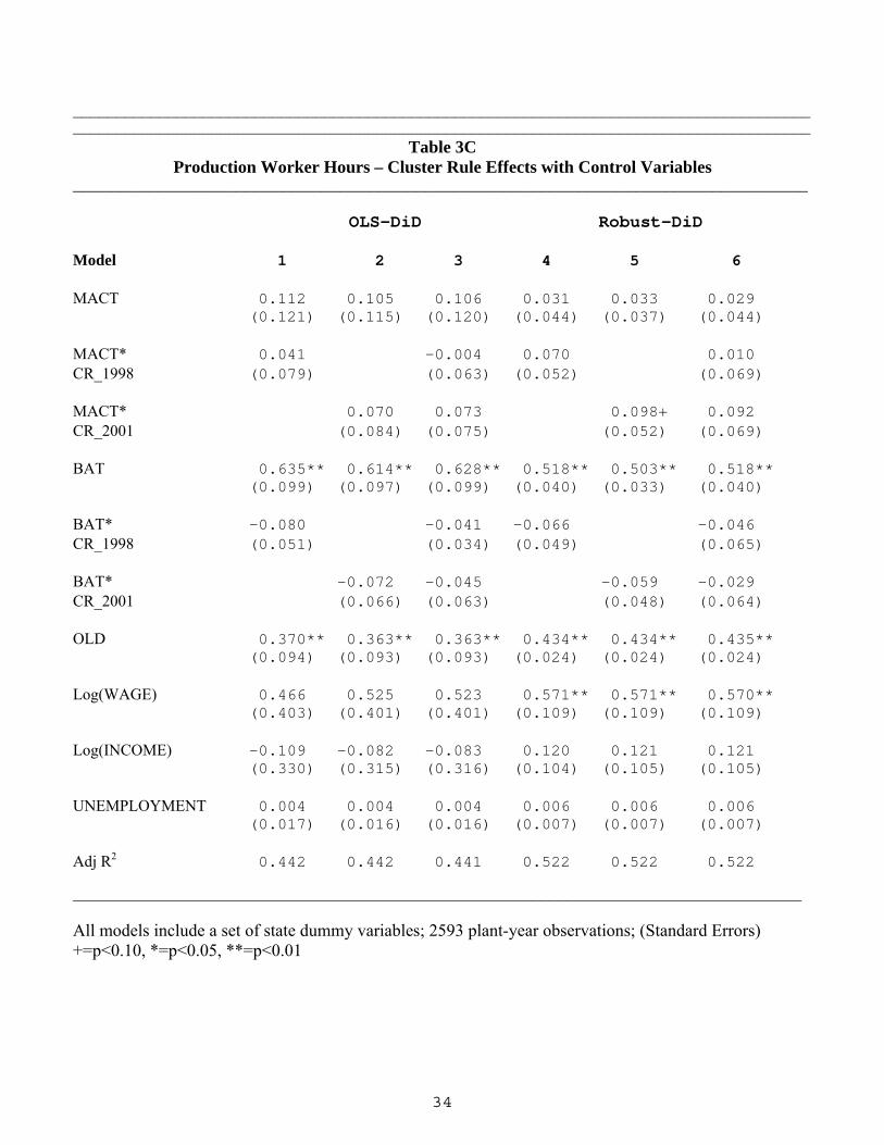
In Tables 3A-3C we turn to models based on equation (6), which include a series of

control variables, including the OLD dummy and various county labor market characteristics.

The control variables give similar results for all three employment measures. Older plants show

about 40% higher employment for all three measures. Plants in high-wage counties have higher

employment, with similar magnitudes in both the regular and robust models, although only the 15 Implemented using the rreg procedure in Stata.

22

robust results are statistically significant. Neither county per-capita income nor county

unemployment rates are significant, though the signs are similar for all three employment

measures. Adding the control variables had essentially no impact on any of the other variables in

the model, with employment at MACT-only plants rising in the post-CR period relative to the

control group, while employment at BAT plants is lower (sometimes significantly so), and

roughly comparable to employment at plants in the control group.

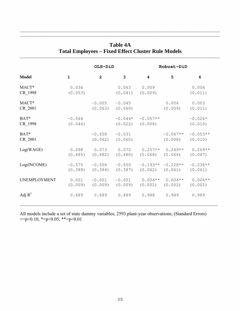
In Tables 4A-4C we now turn to fixed-effect models, based on equation (7), that control

for any differences across plants that remain fixed through our sample period. As noted earlier,

these models cannot include any variables that remain fixed, such as OLD, MACT, and BAT.

The county-level labor market variables now depend on within-county variation over time, not

variation across counties, and are only significant in the robust models, although the signs are

consistent between the regular and robust models. As in Table 3, wage and unemployment rates

are positively associated with employment, while per-capita income is negatively related to

employment.

For the key DiD interaction coefficients, the main difference compared with the results in

Tables 2 and 3 is that the post-CR coefficients for MACT plants are smaller and not always

positive, indicating that their employment experience is not much different from the plants in the

control group. The post-CR MACT coefficients also tend to be more negative for the 2001

cutoff than for the 1998 cutoff, which may reflect relatively little anticipatory investment at those

plants before the CR effective date. The negative post-CR coefficients for BAT plants are

somewhat smaller in magnitude than those in Tables 2 and 3, but the reduction in the MACT

coefficients is larger, so the net (MACT+BAT) effects are more negative than in the earlier

tables. The change is especially pronounced for the robust models, which had shown mostly

23

positive (though insignificant) effects for BAT plants in the earlier tables. They now show

statistically significant reductions of 3%-7% in employment at BAT plants in the post-CR

period, with the effects on total employment being slightly larger than on the production worker

related measures.16

A potential concern with the DiD estimator is that it is most suitable when the treatment

is random, or when observable characteristics can be used to adjust for selection into treatment.

In our case, the MACT and BAT regulations are not randomly assigned to pulp and paper mills.

Rubin (2008) notes that one can approximate a randomized experiment by selecting a suitably-

matched control group to eliminate or at least reduce this bias. In our case, we can reduce

selection bias due to differences in observable covariates by choosing a control group with

comparable covariate distributions to the pulp and paper mills covered by the MACT and BAT

portions of the CR (Stuart (2010)). To choose such a control group we use a version of the

propensity score matching (PSM) estimator developed by Rosenbaum and Rubin (1983). 17

Because we have two treatment groups (MACT-only and BAT) we ran the matching twice -

once for each group. The same set of control plants was used for each matching (with

replacement) and the final dataset included the matched pairs of treatment and control plants.

We tested a variety of specifications before achieving the desired “balance” of matching

variables between our treatment and control groups. The final matching model for the BAT

group included the plant’s energy cost ratio and age, the county unemployment rate, and an

index of the state’s pro-environmental Congressional voting. The matching model for the

MACT-only group included the same variables plus the county non-attainment status for PM,

16 We estimated a set of comparable models using the log of output as the dependent variable and the results are qualitatively similar to the employment results. 17 To estimate the propensity score and produce our matched control group we employ the psmatch2 algorithm in Stata, developed by Leuven and Sianesi (2003).

24

SO2, and NOx and county log income.

Unfortunately, while the DiD estimator with matching provides us with a more

appropriate control group, it also changes our sample as a few treatment plants (and about one-

third of the control plants) are not included in the matched sample. This raises complications for

releasing those results due to Census Bureau rules designed to protect data confidentiality.

However, the estimated effects of MACT and BAT on employment in our DiD analysis with

matching estimators are quite similar to our main DiD results presented above, in both

magnitude and significance. This provides us with some assurance that our results are not being

driven by any observable differences between our treatment and control groups.

7. CONCLUDING REMARKS

In this paper we examine the impact of the Cluster Rule on employment at plants in the

pulp and paper industry. The Cluster Rule, promulgated in the end of 1997 was EPA’s first

integrated, multi-media regulation. Using a sample of pulp and paper mills, we use a DiD

approach to estimate the causal effect of the Cluster Rule on employment. We consider

alternative starting points for the post-CR period (1998 and 2001), alternative measures of

employment (total employment, number of production workers, and production worker hours),

and both regular and robust estimators.

Our results suggest that the Cluster Rule had relatively small effects on employment, with

different effects for plants covered by only the MACT air requirements as compared to plants

that were also covered by the BAT water requirements. The MACT-only plants show small

positive employment effects post-CR in most models, though these are often insignificant. In

contrast, the BAT plants show small negative employment effects relative to the MACT-only

25

plants and (in some models) relative to the control group, also often insignificant. For our final

preferred models, which include plant-specific fixed effects and other control variables, the

robust estimator shows statistically significantly, yet moderately lower employment for the BAT

plants as compared to both the MACT-only plants and the control group. In particular, BAT

plants have on the order of 3%-7% less employment than the control group (the non-robust

results are similar in magnitude, but not significant).

These results should be interpreted with some degree of caution. As noted, most of the

models we estimated had insignificant coefficients on the DiD term measuring the CR effects.

Despite our efforts to develop an appropriate control group (including our confirming the results

with matching DiD estimators), there could still remain some issues of comparability of

treatment and control plants. Future research is needed to link an employment analysis of the

sort conducted here with other measures of the plant’s activities (both in terms of emissions and

production), to get a more complete picture of how the Cluster Rule affected pulp and paper

mills.

26

REFERENCES

Berman, Eli, and Linda T. Bui, (2001a) “Environmental Regulation and Labor Demand: Evidence from the South Coast Air Basin,” Journal of Public Economics, 79, 265 – 295. Berman Eli and Linda Bui, (2001b) “Environmental regulation and productivity: evidence from oil refineries.” Review of Economics and Statistics 83:498–510. Bertrand, M, E. Duflo, and S. Mullainathan, (2004) “How Much Should We Trust difference-in-differences Estimates?” The Quarterly Journal of Economics, vol. 119(1), pp. 249-275. Boyd GA, McClelland JD (1999) “The impact of environmental constraints on productivity improvement in integrated paper plants.” Journal of Environmental Economics and Management 38:121–142. Cole, Mathew and Rob J. Elliott. (2007) “Do Environmental Regulations Cost Jobs? An Industry-Level Analysis of the UK” The B.E. Journal of Economic Analysis and Policy vol 7. issue 1 (Topics) Färe, Rolf, Shawna Grosskopf and Carl Pasurka Jr. (1986) “Effects on Relative Efficiency in Electric Power Generation Due to Environmental Controls” Resources and Energy, Vol. 8, No. 2, (June 1986), 167-184. Gray, Wayne B. and Ronald J. Shadbegian. (1998) “Environmental Regulation, Investment Timing, and Technology Choice” Journal of Industrial Economics, 46, 235-56. Gray, Wayne B. and Ronald J. Shadbegian, (2003) “Plant Vintage, Technology, and Environmental Regulation”, Journal of Environmental Economics and Management, 384-402. Gray, W.B. and R.J. Shadbegian. (2008). “Regulatory Regime Changes Under Federalism: Do States Matter More?”, presented at First Annual Meeting of the Society for Benefit-Cost Analysis.

Gray, W.B. and R.J. Shadbegian. (forthcoming Summer 2013). “Do the Job Effects of Regulation Differ with the Competitive Environment?” Jobs and Regulation edited by Cary Coglianese, Adam Finkel & Chris Carrigan, University of Pennsylvania Press Greenstone, M. (2002). “The Impacts of Environmental Regulations on Industrial Activity: Evidence from the 1970 and 1977 Clean Air Act Amendments and the Census of Manufactures.” Journal of Political Economy 110(6): 1175–1219. Jarmin, R. and Miranda, J. (2002), “The Longitudinal Business Database," CES Working Paper CES-WP-02-17, U.S. Census Bureau, Center for Economic Studies. Laplante, Benoit and Paul Rilstone. (1996). “Environmental Inspections and Emissions of the Pulp and Paper Industry in Quebec,” Journal of Environmental Economics and Management, 31, 19-36.

27

Leuven, E. and Sianesi, B. (2003). psmatch2: Stata module to perform full Mahalanobis and propensity score matching, common support graphing, and covariate imbalance testing. http://ideas.repec.org/c/boc/bocode/s432001.html . Lockwood-Post Pulp and Paper Directory, Miller-Freeman Publishing Company, various issues. Magat, Wesley A. and W. Kip Viscusi. (1990). “Effectiveness of the EPA's Regulatory Enforcement: The Case of Industrial Effluent Standards,” Journal of Law and Economics, 33, 331-360. Morgenstern, Richard D., William A. Pizer, and Jhih-Shyang Shih, (2002) “Jobs Versus the Environment: An Industry-Level Perspective” Journal of Environmental Economics and Management 43, , 412–436. Rosenbaum, P. and Rubin, D. (1983). The central role of the propensity score in observational studies for causal effects. Biometrika 70: 41–55. Rubin, D. (2008). For objective causal inference, design trumps analysis. The Annals of Applied Statistics 2: 808–840. Shadbegian, Ronald J. and Wayne B. Gray, (2003) "What Determines Environmental Performance at Paper Mills? The Roles of Abatement Spending, Regulation, and Efficiency" Topics in Economic Analysis & Policy, http://www.bepress.com/bejeap/topics/vol3/iss1/art15. Shadbegian, R.J. and W.B. Gray. (2005). Pollution Abatement Expenditures and Plant-Level Productivity: A Production Function Approach. Ecological Economics, 54, 196-208. Shadbegian, R.J. and W.B. Gray. (2006). Assessing Multi-Dimensional Performance: Environmental and Economic Outcomes. Journal of Productivity Analysis, 26, 213-234. Stuart, E. (2010). Matching methods for causal inference: A review and a look forward. Statistical Science 25: 1–21. Walker, R. (2011). Environmental Regulation and Labor Reallocation. American Economic Review: Papers and Proceedings 101: 442-447.

28

____________________________________________________________________________________________________________ ____________________________________________________________________________________________________________

Table 1 Descriptive Statistics (1993-2007, N=2593)

____________________________________________________________________________________________________________ Variable Mean (std dev) Description TE 618.63 (405.16) Average employment at plant - Census PW 482.40 (319.51) Average production workers at plant - Census PH 1040.82 (698.61) Annual production worker hours at plant, in 000s - Census LOGTE 6.20 (0.74) Log(TE) LOGPW 5.94 (0.76) Log(PW) LOGPH 6.71 (0.76) Log(PH) MACT 0.68 (0.47) Dummy variable =1 if the plant is covered by EPA Cluster Rule MACT requirements BAT 0.43 (0.49) Dummy variable =1 if the plant is covered by EPA Cluster Rule BAT requirements MACT*CR_1998 0.43 (0.49) Dummy variable =1 after 1997 for plants covered by EPA Cluster Rule MACT requirements MACT*CR_2001 0.29 (0.45) Dummy variable =1 after 2000 for plants covered by EPA Cluster Rule MACT requirements BAT*CR_1998 0.27 (0.44) Dummy variable =1 after 1997 for plants covered by EPA Cluster Rule BAT requirements BAT*CR_2001 0.18 (0.39) Dummy variable =1 after 2000 for plants covered by EPA Cluster Rule BAT requirements OLD 0.74 (0.44) Dummy variable =1 if the plant was in operation in 1960 INCOME 23834 (5779) Average per-capita income in county - BEA WAGE 27957 (5226) Average per-job wages in county - BEA LOG(INCOME) 10.05 (0.24) Log of income LOG(WAGE) 10.22 (0.18) Log(Average per-job wage in county)- BEA UNEMPLOYMENT 6.17 (2.16) Unemployment rate in county - BLS

29

_____________________________________________________________________________________ _____________________________________________________________________________________

Table 2A Total Employees - Only Cluster Rule Effects

_____________________________________________________________________________________ OLS-DiD Robust-DiD Model 1 2 3 4 5 6 MACT 0.096 0.102 0.096 0.016 0.026 0.015 (0.118) (0.113) (0.118) (0.047) (0.039) (0.047) MACT* 0.058 0.018 0.105+ 0.032 CR_1998 (0.075) (0.061) (0.056) (0.075) MACT* 0.071 0.059 0.130* 0.110 CR_2001 (0.080) (0.073) (0.055) (0.074) BAT 0.637** 0.619** 0.637** 0.589** 0.571** 0.590** (0.097) (0.095) (0.097) (0.043) (0.035) (0.043) BAT* -0.094+ -0.051+ -0.103+ -0.053 CR_1998 (0.050) (0.031) (0.053) (0.071) BAT -0.096 -0.063 -0.107* -0.073 CR_2001 (0.064) (0.064) (0.052) (0.069) Adj R2 0.426 0.426 0.425 0.458 0.459 0.458 _____________________________________________________________________________

All models include a set of state dummy variables; 2593 plant-year observations; (Standard Errors) +=p<0.10, *=p<0.05, **=p<0.01

30

_____________________________________________________________________________________

Table 2B Production Workers – Only Cluster Rule Effects

_____________________________________________________________________________________ OLS-DiD Robust-DiD Model 1 2 3 4 5 6 MACT 0.114 0.116 0.114 0.034 0.041 0.033 (0.121) (0.115) (0.121) (0.048) (0.041) (0.048) MACT* 0.039 0.005 0.080 0.022 CR_1998 (0.080) (0.064) (0.058) (0.077) MACT* 0.053 0.050 0.101+ 0.087 CR_2001 (0.085) (0.076) (0.057) (0.076) BAT 0.629** 0.610** 0.629** 0.570** 0.551** 0.571** (0.099) (0.097) (0.099) (0.045) (0.037) (0.045) BAT* -0.084+ -0.055+ -0.087 -0.056 CR_1998 (0.050) (0.031) (0.055) (0.073) BAT* -0.079 -0.044 -0.081 -0.046 CR_2001 (0.065) (0.065) (0.053) (0.071) Adj R2 0.404 0.404 0.403 0.440 0.440 0.439 ____________________________________________________________________________________

All models include a set of state dummy variables; 2593 plant-year observations; (Standard Errors) +=p<0.10, *=p<0.05, **=p<0.01

31

_____________________________________________________________________________________

Table 2C Production Worker Hours - Only Cluster Rule Effects

_____________________________________________________________________________________

OLS-DiD Robust-DiD Model 1 2 3 4 5 6 MACT 0.104 0.100 0.104 0.033 0.033 0.032 (0.120) (0.114) (0.120) (0.048) (0.040) (0.048) MACT* 0.043 -0.010 0.067 0.002 CR_1998 (0.080) (0.066) (0.057) (0.077) MACT* 0.072 0.079 0.100+ 0.099 CR_2001 (0.084) (0.075) (0.057) (0.076) BAT 0.626** 0.611** 0.626** 0.566** 0.549** 0.567** (0.098) (0.096) (0.098) (0.044) (0.036) (0.044) BAT* -0.077 -0.043 -0.073 -0.048 CR_1998 (0.053) (0.035) (0.054) (0.072) BAT* -0.078 -0.050 -0.066 -0.035 CR_2001 (0.066) (0.064) (0.053) (0.071) Adj R2 0.405 0.405 0.405 0.443 0.443 0.443 ____________________________________________________________________________________

All models include a set of state dummy variables; 2593 plant-year observations; (Standard Errors) +=p<0.10, *=p<0.05, **=p<0.01

32

__________________________________________________________________________________________________________________________________________________________________________

Table 3A Total Employees – Cluster Rule Effects with Control Variables

_____________________________________________________________________________________ OLS-DiD Robust-DiD Model 1 2 3 4 5 6 MACT 0.098 0.106 0.098 -0.009 -0.001 -0.013 (0.120) (0.116) (0.120) (0.043) (0.036) (0.043) MACT* 0.060 0.024 0.100* 0.027 CR_1998 (0.074) (0.059) 0.051) (0.068) MACT* 0.069 0.054 0.128* 0.110 CR_2001 (0.080) (0.073) (0.050) (0.067) BAT 0.640** 0.622** 0.640** 0.562** 0.544** 0.562** (0.098) (0.096) (0.099) (0.040) (0.033) (0.039) BAT* -0.089+ -0.049 -0.102* -0.052 CR_1998 (0.050) (0.031) (0.048) (0.064) BAT* -0.090 -0.058 -0.108* -0.075 CR_2001 (0.064) (0.063) (0.047) (0.062) OLD 0.331** 0.331** 0.331** 0.410** 0.412** 0.414** (0.093) (0.093) 0.093) (0.024) (0.024) (0.024) Log(WAGE) 0.462 0.463 0.462 0.471** 0.474** 0.473** (0.398) (0.398) (0.398) (0.106) (0.106) (0.106) Log(INCOME) -0.045 -0.047 -0.048 0.113 0.111 0.113 (0.320) (0.320) (0.320) (0.102) (0.102) (0.102) UNEMPLOYMENT 0.005 0.005 0.005 0.005 0.006 0.006 0.017) (0.017) (0.017) (0.007) (0.007) (0.007) Adj R2 0.458 0.458 0.458 0.540 0.541 0.542 ____________________________________________________________________________________

All models include a set of state dummy variables; 2593 plant-year observations; (Standard Errors) +=p<0.10, *=p<0.05, **=p<0.01

33

__________________________________________________________________________________________________________________________________________________________________________

Table 3B Production Workers – Cluster Rule Effects with Control Variables

_____________________________________________________________________________

OLS-DiD Robust-DiD Model 1 2 3 4 5 6 MACT 0.112 0.115 0.111 0.029 0.036 0.028 (0.121) (0.116) (0.122) (0.044) (0.037) (0.044) MACT* 0.041 0.010 0.075 0.022 CR_1998 (0.079) (0.062) (0.053) (0.070) MACT* 0.053 0.046 0.095+ 0.081 CR_2001 (0.085) (0.076) (0.052) (0.069) BAT 0.635** 0.616** 0.635** 0.530** 0.512** 0.531** (0.099) (0.097) (0.099) (0.041) (0.034) (0.041) BAT* -0.080 -0.053+ -0.083+ -0.055 CR_1998 (0.051) (0.031) (0.050) (0.066) BAT* -0.075 -0.040 -0.077 -0.041 CR_2001 (0.065) (0.064) (0.049) (0.065) OLD 0.370** 0.370** 0.370** 0.437** 0.436** 0.437** (0.094) (0.094) (0.094) (0.024) (0.024) (0.024) Log(WAGE) 0.466 0.468 0.466 0.509** 0.509** 0.508** (0.403) (0.403) (0.403) (0.110) (0.110) (0.110) Log(INCOME) -0.109 -0.110 -0.111 0.098 0.096 0.097 (0.330) (0.330) (0.330) (0.105) (0.105) (0.105) UNEMPLOYMENT 0.004 0.004 0.004 0.005 0.005 0.005 (0.017) (0.017) (0.017) (0.007) (0.007) (0.007) Adj R2 0.441 0.441 0.441 0.518 0.518 0.518 ____________________________________________________________________________________ All models include a set of state dummy variables; 2593 plant-year observations; (Standard Errors) +=p<0.10, *=p<0.05, **=p<0.01

34

__________________________________________________________________________________________________________________________________________________________________________

Table 3C Production Worker Hours – Cluster Rule Effects with Control Variables

_____________________________________________________________________________

OLS-DiD Robust-DiD Model 1 2 3 4 5 6 MACT 0.112 0.105 0.106 0.031 0.033 0.029 (0.121) (0.115) (0.120) (0.044) (0.037) (0.044) MACT* 0.041 -0.004 0.070 0.010 CR_1998 (0.079) (0.063) (0.052) (0.069) MACT* 0.070 0.073 0.098+ 0.092 CR_2001 (0.084) (0.075) (0.052) (0.069) BAT 0.635** 0.614** 0.628** 0.518** 0.503** 0.518** (0.099) (0.097) (0.099) (0.040) (0.033) (0.040) BAT* -0.080 -0.041 -0.066 -0.046 CR_1998 (0.051) (0.034) (0.049) (0.065) BAT* -0.072 -0.045 -0.059 -0.029 CR_2001 (0.066) (0.063) (0.048) (0.064) OLD 0.370** 0.363** 0.363** 0.434** 0.434** 0.435** (0.094) (0.093) (0.093) (0.024) (0.024) (0.024) Log(WAGE) 0.466 0.525 0.523 0.571** 0.571** 0.570** (0.403) (0.401) (0.401) (0.109) (0.109) (0.109) Log(INCOME) -0.109 -0.082 -0.083 0.120 0.121 0.121 (0.330) (0.315) (0.316) (0.104) (0.105) (0.105) UNEMPLOYMENT 0.004 0.004 0.004 0.006 0.006 0.006 (0.017) (0.016) (0.016) (0.007) (0.007) (0.007) Adj R2 0.442 0.442 0.441 0.522 0.522 0.522 ____________________________________________________________________________________ All models include a set of state dummy variables; 2593 plant-year observations; (Standard Errors) +=p<0.10, *=p<0.05, **=p<0.01

35

__________________________________________________________________________________________________________________________________________________________________________

Table 4A Total Employees – Fixed Effect Cluster Rule Models

_____________________________________________________________________________________ OLS-DiD Robust-DiD Model 1 2 3 4 5 6 MACT* 0.036 0.063 0.009 0.006 CR_1998 (0.053) (0.041) (0.009) (0.011) MACT* -0.005 -0.045 0.006 0.003 CR_2001 (0.063) (0.060) (0.009) (0.011) BAT* -0.064 -0.044* -0.057** -0.026* CR_1998 (0.046) (0.022) (0.008) (0.010) BAT* -0.058 -0.031 -0.067** -0.053** CR_2001 (0.062) (0.060) (0.008) (0.010) Log(WAGE) 0.098 0.073 0.072 0.257** 0.269** 0.269** (0.485) (0.482) (0.480) (0.068) (0.066) (0.067) Log(INCOME) -0.575 -0.558 -0.550 -0.193** -0.228** -0.238** (0.388) (0.384) (0.387) (0.062) (0.061) (0.061) UNEMPLOYMENT 0.001 -0.001 -0.001 0.004** 0.004** 0.004** (0.009) (0.009) (0.009) (0.002) (0.002) (0.002) Adj R2 0.889 0.889 0.889 0.988 0.989 0.989 ____________________________________________________________________________________ All models include a set of state dummy variables; 2593 plant-year observations; (Standard Errors) +=p<0.10, *=p<0.05, **=p<0.01

36

__________________________________________________________________________________________________________________________________________________________________________

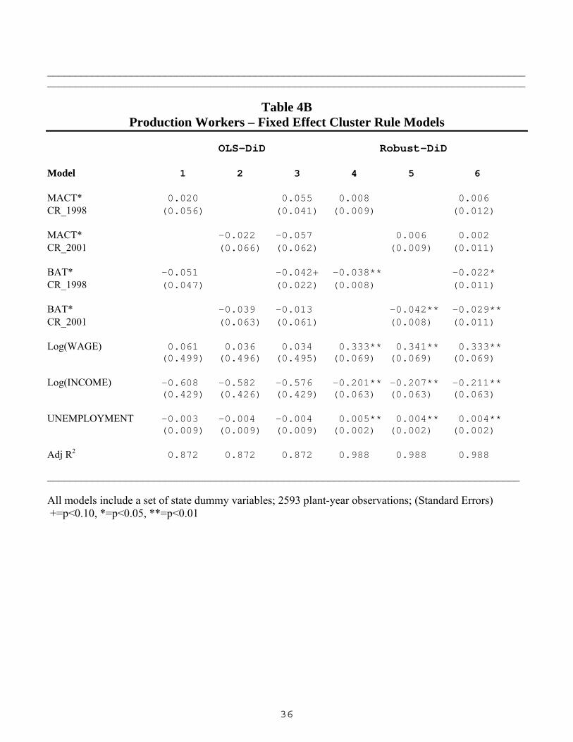
Table 4B Production Workers – Fixed Effect Cluster Rule Models

OLS-DiD Robust-DiD Model 1 2 3 4 5 6 MACT* 0.020 0.055 0.008 0.006 CR_1998 (0.056) (0.041) (0.009) (0.012) MACT* -0.022 -0.057 0.006 0.002 CR_2001 (0.066) (0.062) (0.009) (0.011) BAT* -0.051 -0.042+ -0.038** -0.022* CR_1998 (0.047) (0.022) (0.008) (0.011) BAT* -0.039 -0.013 -0.042** -0.029** CR_2001 (0.063) (0.061) (0.008) (0.011) Log(WAGE) 0.061 0.036 0.034 0.333** 0.341** 0.333** (0.499) (0.496) (0.495) (0.069) (0.069) (0.069) Log(INCOME) -0.608 -0.582 -0.576 -0.201** -0.207** -0.211** (0.429) (0.426) (0.429) (0.063) (0.063) (0.063) UNEMPLOYMENT -0.003 -0.004 -0.004 0.005** 0.004** 0.004** (0.009) (0.009) (0.009) (0.002) (0.002) (0.002) Adj R2 0.872 0.872 0.872 0.988 0.988 0.988 ____________________________________________________________________________________ All models include a set of state dummy variables; 2593 plant-year observations; (Standard Errors) +=p<0.10, *=p<0.05, **=p<0.01

37

__________________________________________________________________________________________________________________________________________________________________________

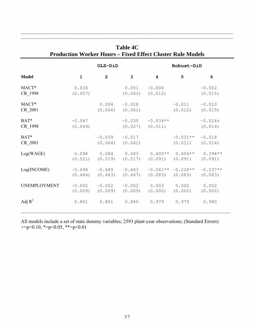
Table 4C Production Worker Hours – Fixed Effect Cluster Rule Models

OLS-DiD Robust-DiD

Model 1 2 3 4 5 6 MACT* 0.034 0.051 -0.006 -0.002 CR_1998 (0.057) (0.043) (0.012) (0.015) MACT* 0.004 -0.028 -0.011 -0.010 CR_2001 (0.066) (0.061) (0.012) (0.015) BAT* -0.047 -0.035 -0.034** -0.024+ CR_1998 (0.049) (0.027) (0.011) (0.014) BAT* -0.039 -0.017 -0.031** -0.018 CR_2001 (0.064) (0.061) (0.011) (0.014) Log(WAGE) 0.098 0.084 0.083 0.400** 0.404** 0.394** (0.521) (0.519) (0.517) (0.091) (0.091) (0.091) Log(INCOME) -0.698 -0.689 -0.683 -0.241** -0.228** -0.237** (0.466) (0.463) (0.467) (0.083) (0.083) (0.083) UNEMPLOYMENT -0.002 -0.002 -0.002 0.003 0.002 0.002 (0.009) (0.009) (0.009) (0.002) (0.002) (0.002) Adj R2 0.861 0.861 0.860 0.979 0.979 0.980 ____________________________________________________________________________________ All models include a set of state dummy variables; 2593 plant-year observations; (Standard Errors) +=p<0.10, *=p<0.05, **=p<0.01

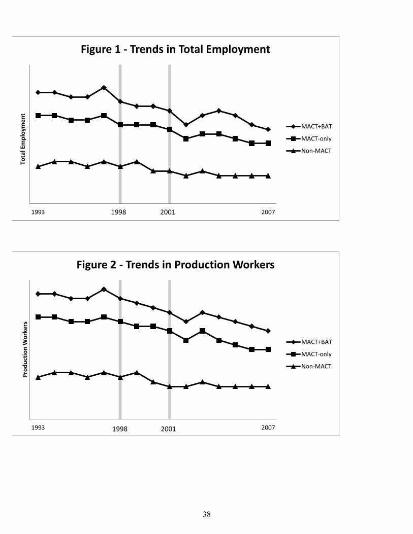
1993 2007

Tota

l Em

plo

yme

nt

Figure 1 - Trends in Total Employment

MACT+BAT

MACT-only

Non-MACT

1998 2001

1993 2007

Pro

du

ctio

n W

ork

ers

Figure 2 - Trends in Production Workers

MACT+BAT

MACT-only

Non-MACT

1998 2001

38

1993 2007

Pro

du

ctio

n W

ork

er

Ho

urs

Figure 3 - Trends in Production Worker Hours

MACT+BAT

MACT-only

Non-MACT

1998 2001

39