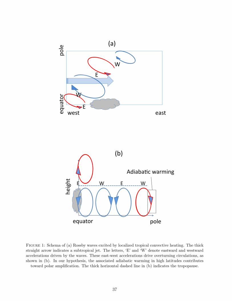
Do Planetary Wave Dynamics Contribute to

Equable Climates?

Sukyoung Leea, Steven Feldsteina, David Pollardb, and Tim Whiteb

a Department of Meteorology, The Pennsylvania State University, University Park,

Pennsylvania

b Earth and Environment Systems Institute, The Pennsylvania State University,

University Park, Pennsylvania

December 19, 2010

Corresponding author address: Dr. Sukyoung Lee, Department of Meteorology, The

Pennsylvania State University, University Park, Pennsylvania 16802, USA. E-mail:

sl@meteo.psu.edu

Abstract

Viable explanations for equable climates of the Cretaceous and early Cenozoic (about

145 to 50 million years ago), especially for the above-freezing temperatures detected for

high-latitude continental winters, have been a long-standing challenge. In this study, we

suggest that enhanced and localized tropical convection, associated with a strengthened

paleo warm pool, may contribute toward high-latitude warming through the excitation of

poleward propagating Rossby waves. This warming takes place through the poleward heat

flux and an overturning circulation that accompany the Rossby waves. This mechanism is

tested with an atmosphere-mixed layer ocean general circulation model (GCM) by imposing

idealized localized heating and compensating cooling, a heating structure which mimics the

effect of warm pool convective heating.

The localized tropical heating is indeed found to contribute to a warming of the Arctic

during the winter. Within the range of 0− 150 Wm−2 for the heating intensity, the average

rate for the zonal mean Arctic surface warming is 0.8oC per 10Wm−2 increase in the heating

for the runs with an atmospheric CO2 level of 4×PAL (Preindustrial Atmospheric Level, 1

PAL = 280 ppmv), the Cretaceous and early Cenozoic values considered for this study. This

rate of warming for the Arctic is lower in model runs with 1 × PAL CO2, which show an

increase of 0.3oC per 10 Wm−2. Further increase of the heating intensity beyond 150 Wm−2

produces little change in the Arctic surface air temperature. This saturation behavior is

interpreted as being a result of nonlinear wave-wave interaction which leads to equatorward

wave refraction.

Under the 4 × PAL CO2 level, raising the heating from 120 Wm−2 (estimated warm

1

pool convective heating value for the present-day climate) to 150 Wm−2 and 180 Wm−2

(estimated values for the Cretaceous and early Cenozoic) produces a warming of 4oC − 8oC

over northern Siberia and the adjacent Arctic Ocean. Relative to the warming caused by a

quadrupling of CO2 alone, this temperature increase accounts for about 30% of the warming

over this region. The possible influence of warm pool convective heating on the present-day

Arctic is also discussed.

2

1 Introduction

Proxy data indicate that climates during the Cretaceous and early Cenozoic (from about

145 to 50 million years ago) were more equable than the present-day climate, with smaller

latitudinal variations in surface air temperature (Huber 2008; Spicer et al. 2008). The

primary suspect is higher levels of greenhouse gases. General circulation model (GCM)

experiments show that CO2 levels of at least 10× PAL (Preindustrial Atmospheric Level,

1 PAL = 280 ppmv) are needed to produce the observed high-latitude continental winter

warmth (e.g., Bice et al. 2006; Poulsen et al. 2008; Hunter et al. 2008), but these levels

significantly exceed those of recent proxy estimates for the Cretaceous and early Cenozoic:

≈ 4− 8× PAL (Bice et al. 2006); 4× PAL (Fletcher et al. 2008).

Mechanisms proposed to date include an enhanced poleward oceanic heat transport (e.g.,

Barron et al. 1993; Sloan et al. 1995), a warming caused by substantially greater polar

stratospheric cloud cover (Sloan and Pollard 1998; Sloan et al. 1999, Kirk-Davidoff et al.

2002), a greatly expanded Hadley cell (Farrell 1990), a convection-cloud radiative forcing

(CCRF) feedback (Sewall and Sloan 2004; Abbot and Tziperman 2008a,b), a vegetation-

climate feedback (Otto-Bliesner and Upchurch 1997; DeConto et al. 2000), an intensification

of the thermohaline circulation due to driving by tropical cyclones (Sriver and Huber 2007;

Korty et al. 2008), and decreased cloud reflectivity due to a reduction in the number of

cloud condensation nuclei (Kump and Pollard 2008).

In this study, we propose and then test the mechanism that enhanced and localized trop-

ical convection can also trigger high-latitude warming through the excitation of poleward

propagating planetary-scale Rossby waves which transport heat poleward and induce sink-

3

ing motions. Our proposed mechanism is based on the premise that under the high CO2

loading conditions, tropical convection was more intense and localized during the Cretaceous

and early Cenozoic than it is for the present-day climate. The rationale for this premise is

that as the tropical sea surface temperature (SST) increases, due to the higher CO2 load-

ing, tropical convection over the western part of the largest ocean basin (the warm pool,

hereafter) will intensify more rapidly than elsewhere because saturation vapor pressure is

an exponential function of temperature (the Clausius-Clapeyron equation). Based on the

Clausius-Clapeyron relation, Held and Soden (2006) formulated a scaling for the sensitivity

of precipitation minus evaporation (P−E) to surface temperature change. In response to a

surface temperature increase, their theoretical prediction shows that the largest increase in

P-E occurs over the Indian and western Pacific Oceans. While increased CO2 radiatively

warms all latitudes, the proposed mechanism leads to a further warming at high latitudes

and a cooling of the tropics through the heat transport and overturning circulation associated

with the poleward propagating waves.

Lee et al. (2010) examined the tropical precipitation trend for the months of December

through February (DJF) over the time period of 1979-2002, using the Global Precipitation

Climatology Project (GPCP), Climate-Prediction-Center Merged Analysis of Precipitation

(CMAP), and European Center for Medium-Range Weather Forecasts reanalysis data (ERA-

40) datasets. Their Fig. 1 shows that the most pronounced positive trend occurred over the

Indo-western Pacific warm pool region. Although other processes may be involved in the

changes shown in that figure, since the surface air temperature has increased during this time

period, the Indo-western Pacific warm pool intensification of the convective precipitation is

at least consistent with the theoretical expectation based on the Clausius-Clapeyron relation.

4

Because the core of our proposed mechanism hinges on a warmer tropical SST during the

Cretaceous and early Cenozoic, this mechanism may also be applicable for climates under

other conditions, such as that characterized by stronger solar radiation, as long as it causes

the tropical SSTs to increase.

To the best of our knowledge, there are no paleotemperature estimates available for the

Indian and western Pacific Oceans. However, paleotemperature estimates from the western

Atlantic at the Demerara Rise during the Cenomanian-Turonian period (Forster et al. 2007)

indicate values that range between 32oC and 43oC, with a typical value of 36oC − 37oC.

Therefore, if we assume that a similar SST increase relative to the present-day climate

occurred in other tropical oceans, and that a warm pool existed in the western part of the

paleo Pacific ocean, as in the present-day climate, these paleotemperature estimates suggest

that the SSTs in the western Pacific warm pool region were higher than the present-day

values by at least 6oC, and perhaps as much as 13oC. While the precise SST values differ

between Cretaceous simulations, Bush and Philander (1997) and Otto-Bliesner et al. (2002)

support the assumption that the warmest SSTs would have occurred over the paleo western

Pacific Ocean.

One advantage of the proposed mechanism is that it is at best only weakly dependent

upon the equator-to-pole temperature gradient. As a result, if enhanced and localized trop-

ical convection takes place, it can readily generate a high-latitude warming in the presence

of a wide range of background equator-to-pole temperature gradients.

In section 2, we advance the theoretical and empirical basis for this mechanism. The

GCM employed for this study will be described in section 3 and the experimental design is

discussed in section 4. The results are presented in sections 5 through 7, and the conclusions

5

follow in section 8.

2 Mechanism: planetary wave dynamics as the warm-

ing mechanism

The mechanism that we propose is that enhanced and localized tropical convection is ca-

pable of generating planetary-scale Rossby waves which, through the attendant poleward

heat flux and overturning circulation (refer to Fig. 1), can trigger high latitude warming.

This overturning circulation associated with poleward Rossby wave propagation needs fur-

ther explanation. For Rossby waves, the poleward propagation out of the tropics must be

accompanied by a transport of eastward angular momentum toward the tropics (for external

Rossby waves, the angular momentum transport is always in a direction opposite to that

of the wave propagation (Held 1975)). This angular momentum transport results in a force

imbalance, and as a response, an overturning circulation develops with sinking motion at

higher latitudes and rising motion at lower latitudes. This process of inducing vertical mo-

tions, which is ubiquitous throughout the atmosphere, is known as thermal wind adjustment

(e.g., Holton 2004). The impact of these vertical motions is to adiabatically warm high

latitudes and adiabatically cool midlatitudes (see Fig. 1b).

3 Model Description

This mechanism is tested using a coupled atmosphere-mixed layer ocean GCM that has

a local heat source which is designed to mimic warm pool convective heating. One may

6

question whether a coupled atmosphere-dynamic ocean GCM is more suitable because such

a model can generate internally consistent SST and convective precipitation fields. However,

for our purpose, there are two reasons why a mixed layer ocean model with an idealized

heat source is a better choice than a dynamic ocean model with internally generated warm

pool heating. First, there is the question of model fidelity in simulating the distribution

and intensity of tropical convective precipitation. As was shown by Lin et al. (2006), even

amongst the latest versions of the coupled models which participated in the IPCC AR4,

there is large inter-model scatter in the intensity (a factor of two difference between some

models) of the Indo-Pacific warm pool tropical precipitation.

More importantly, even if we are given a perfect coupled model, with such a model it

is difficult to tease apart the impact of tropically forced atmospheric waves from influences

caused by other processes. For example, changes in the greenhouse gas composition may

influence the extratropical ocean circulation which can also warm the Arctic. According to

the calculations by Trenberth and Caron (2001), the poleward heat transport across 60oN

in the Atlantic Ocean is on the order of 0.5 PW (Petawatts = 1015 W). As Wunsch (2005)

pointed out, while this is a small amount compared with the 4 PW of atmospheric heat

transport across the same latitude, removing or adding 0.5 PW would correspond to an

atmospheric radiative forcing change greater than that from a doubling of atmospheric CO2.

Therefore, if the increase in CO2 can cause the extratropical ocean circulation to change,

and if the coupled model can precisely simulate this process, then it would be difficult to

isolate the effect of the proposed mechanism on the Arctic warming.

Given the above considerations, it is desirable to use a static ocean model for this study.

One viable choice is a mixed-layer ocean model with no ocean currents but with diffusive

7

heat transport. The lack of an explicit ocean circulation means that the model poorly simu-

lates zonally asymmetric oceanic features such as the western warm pool, and the east-west

distribution of tropical convective heating (see Figs. 3a and 3c in Thompson and Pollard

(1997)). For this reason, the intensity of tropical convective heating perturbations is esti-

mated empirically and imposed in the model. An additional advantage of using a mixed-layer

ocean GCM is that many paleoclimate studies in the past have used the same type of model.

If the proposed mechanism turns out to contribute to the polar warming, it indicates that

mixed-layer ocean GCMs may have been underestimating the polar temperature amplifica-

tion. Thus, such a finding can ultimately contribute toward an improvement of paleoclimate

models.

The experiments presented in this study use GENESIS version 2.3, a GCM which is

composed of an atmospheric model coupled to multilayer models of vegetation, soil, land,

ice, and snow (Thompson and Pollard, 1997). Sea-surface temperatures and sea ice are

computed using a 50-m slab oceanic mixed layer with diffusive heat fluxes. The atmospheric

GCM has a T31 spectral resolution (≈ 3.75o) with 18 vertical levels, and the grid for all

surface components is 2o×2o. The GENESIS GCM has been used extensively in paleoclimatic

applications; previous Cretaceous studies include DeConto et al. (2000), Bice et al. (2006),

Poulsen et al. (2007), Zhou et al. (2008), and Kump and Pollard (2008).

For the Cretaceous simulations in this study, the boundary conditions were those used

in Poulsen et al. (2007) for the middle Cretaceous, including Cenomanian paleography

and topography with high sea-level stand, a reduced solar luminosity (1354.4Wm−2), and

a circular orbit with obliquity (23.5o), similar to modern values. A uniform land-surface

corresponding to a savanna biome was specified. The ocean diffusive heat-flux coefficient

8

was set to a value that provides the best simulation of the modern climate.

4 Experimental Design

In light of our aim to test the hypothesis that enhanced and localized tropical heating can

excite Rossby waves which can in turn warm the Arctic, we first perform two types of

model runs: a run with no specified localized tropical heating, and a series of runs with

prescribed localized tropical heatings of varying strength. The latter runs will be referred

to as EXP runs. By comparing these model runs, we are isolating the impact of localized

tropical heating upon the Arctic surface air temperature for a range of plausible tropical

heating values. It is important to keep in mind that this approach has limitations, since it

does not take into account various processes such as the impact of the heating on the ocean

circulation. As such, one should regard the findings of this study as a qualitative assessment

of Arctic warming due to localized tropical heating.

We used the present-day tropical precipitation and heating distribution as a guide for

determining the amplitude and horizontal structure of the heating in the model. Because

our primary focus is on the warming mechanism in the Northern Hemisphere (NH) high

latitudes during the winter, data from the months of December, January, and February

(DJF) are used. For the present-day climate, over the warm pool, the estimated latent

heating from the convective precipitation is approximately 320 Wm−2. Over the rest of the

tropics, the average latent heating is approximately 160 Wm−2. Thus, for the present-day

climate, the warmest part of the tropical ocean is associated with an additional 160 Wm−2

of heating compared with other tropical locations. Because of the larger amount of CO2 in

9

the atmosphere during the Cretaceous and early Cenozoic, as discussed in the introduction,

it would be expected that the warm pool convection during that time period was stronger

and more localized than that of the modern-day climate (Bush and Philander 1997).

For our estimation of the tropical heating, we first assume that the CO2 level for the

Cretaceous and early Cenozoic was 4 × PAL. If the lower tropospheric air temperature

increases by 3oC for every doubling of CO2 (according to the IPCC AR4, most GCMs

predict temperature increases between 2oC and 4.5oC), for an increase of CO2 to 4× PAL,

the temperature would increase by about 6oC. If the precipitation rate increases by 2 % for

every 1oC increase (Held and Soden 2006), then for a CO2 concentration of 4 × PAL, the

precipitation rate would increase by 12 %. If one assumes that this increase occurs uniformly

over the entire tropics, the difference in latent heating between the warm pool and the rest of

the tropical ocean would be about (320 Wm−2 − 160 Wm−2)× 1.12 ≈ 180 Wm−2. Because

most precipitation occurs over the warm pool, if this increase occurs primarily in that region,

then the difference in latent heating between the warm pool and elsewhere would instead be

320 Wm−2 × 1.12 − 160 Wm−2 ≈ 200 Wm−2. This amounts to 25 % increase in the zonal

heating contrast compared with the present value of ≈ 160 Wm−2.

Both SST and tropical precipitation changes associated with present-day climate change

suggest that the above estimate of the increase in the zonal heating contrast is on the

conservative side. Kumar et al. (2010) showed that between 1950 and 2008 the largest

SST increase in the tropics occurred in the Indian and western Pacific Oceans. Thus, our

assumption of a uniform tropical SST increase underestimates this rate. According to the

1979-2002 tropical precipitation trend of Lee et al. (2010), both the GPCP and CMAP

data indicate that over a period of 50 years the trend would result in an increase of about

10

22.5 Wm−2 in the warm pool region and a decrease of 7.5 Wm−2 outside of this region.

Thus, in 50 years, the zonal heating contrast would increase by 30 Wm−2. Relative to

the current-day climatological 160 Wm−2 heating contrast, this amounts to an increase of

19%. Between 1958 and 2010, the CO2 concentration measured at Mauna Loa Observatory

(http://www.esrl.noaa.gov/gmd/ccgg/trends/#mlo full) shows an increase of about 25 %.

Therefore, our estimate of a 25% increase in the zonal heating contrast under a 4 × PAL

CO2 concentration is apparently a very conservative estimate.

Given the uncertainty in the zonal heating contrast that would have existed, and keeping

in mind that the goal of this study is to perform a proof-of-concept test of our proposed

hypothesis, rather than examining the climate response to a single value of the heating

contrast, it would be more reasonable to consider a range of plausible values to examine the

sensitivity of the surface air temperature to the tropical heating. Thus, the values of the

tropical heating, Qo, that we will consider for our EXP runs are: 75 Wm−2, 120 Wm−2,

150 Wm−2, 180 Wm−2, and 225 Wm−2. The corresponding warm pool/outside warm pool

heating contrast is 100 Wm−2, 160 Wm−2, 200 Wm−2, 240 Wm−2, and 300 Wm−2. These

values can be obtained by noting that our ”warm pool” occupies 90 degrees longitude, with

the remainder of the tropics spanning 270 degrees of longitude. For example, for the present-

day case, the zonal mean heating equals (1× 320 Wm−2 + 3× 160 Wm−2)/4 = 200 Wm−2

(see the above discussion). Therefore, the warm-pool additional heating above the zonal

mean is 320 Wm−2 - 200 Wm−2 = 120 Wm−2. While the 120 Wm−2 value is used to

simulate the present-day warm pool, the three higher values are regarded as plausible values

for a 4× PAL atmosphere. The 75 Wm−2 case is considered as an additional data point in

our effort to examine the extent to which the surface air temperature response to the heating

11

is linear.

Atmospheric CO2 levels in these experiments were set to 4× PAL value. For the EXP

runs discussed above, a constant heating term was applied to the GCM atmosphere, with

a vertically integrated column total of Qo. The heating was distributed vertically with

a parabolic dependence on σ (≡ pressure/surface pressure), with non-zero values ranging

between σ = 0.15 and 0.75, and a maximum heating at σ = 0.5. This was applied uniformly

between latitudes 10oS and 10oN , and from longitudes 10oE to 100oE (see the red-boxed

area in Fig. 2), a region approximately akin to the present-day warm pool. For this reason,

although there is no warm pool in the slab ocean, this region will be referred to as a paleo

warm pool. A corresponding cooling with the same vertical profile was applied uniformly

between the same latitudes and throughout all other longitudes (see the blue-boxed area

in Fig. 2), so that the net zonal and global mean heating are zero. For instance, if Qo =

150Wm−2, the heating difference between the heated and cooled region is 200Wm−2. The

values of Qo considered in this study and the corresponding zonal heating contrast are

summarized in Table 1, along with the symbol for each experiment. The symbols are written

as EXPm-n, where m is the CO2 factor relative to PAL and n = Qo(Wm−2). Hereafter,

each experiment will be referred to by its symbol.

The sensitivity of the high latitude surface air temperature to the tropical heating con-

trast will also be examined for 1 × PAL atmosphere. There are reasons why the sensi-

tivity may be dependent on CO2 concentration. For instance, as model calculations of the

present-day climate change indicate, the background atmospheric state changes as the CO2

concentration increases. This change in the background flow would influence the Rossby

wave propagation characteristics, on which our proposed hypothesis is dependent. Different

12

CO2 concentrations can also influence the base-extent of snow and ice, and hence the degree

of albedo feedback, as mentioned later.

Because the goal of this study is to perform a proof-of-concept test of our proposed

hypothesis, we first examine the proposed mechanism by comparing the EXP4-150 (Qo =

150 Wm−2) run against the EXP4-0 run (see Table 1) which has no imposed heating and

cooling, i.e., Qo = 0 Wm−2. This comparison can succinctly illustrate the mechanism by

which localized tropical convection can warm the Arctic. As discussed earlier, because of

the absence of ocean currents in this model, without the added heating, there is essentially

no zonal variation in tropical heating in the EXP4-0 run. In both of the model runs, the

atmospheric CO2 loading is 4× PAL.

After examining the workings of the proposed mechanism in Sections 5 and 6, the results

from the various EXP runs will be presented in Section 7. By inter-comparing the EXP

runs, we will be able to address the extent to which the proposed mechanism can contribute

to the winter Arctic warming.

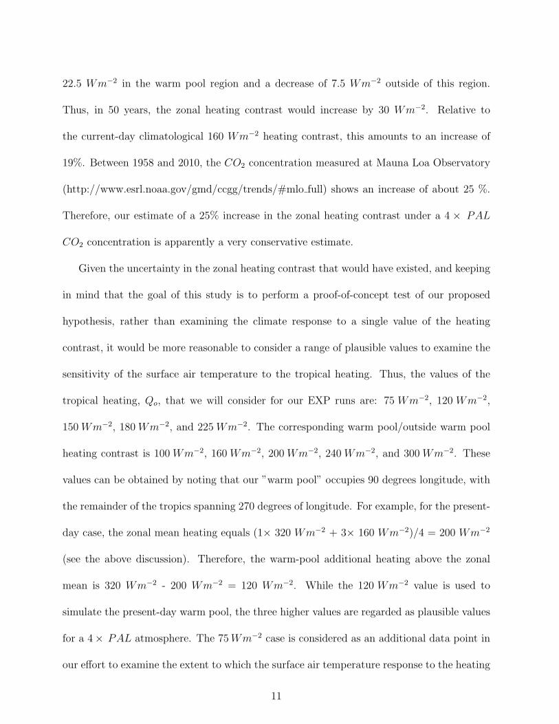
5 Surface warming and stationary wave

The difference in the January surface air temperature at the lowest model level (σ = .933), δT

(Fig. 2), shows warming at high latitudes and an overall cooling in the tropics. (The notation

δF refers to F(EXP4 − 150) − F(EXP4 − 0), where F is a given model variable. Note

that δF is not an estimate of the actual Cretaceous changes relative to the modern world;

the latter is addressed in section 7 and Figs. 8 and 9.) The warming in the Arctic is as high

as 16oC, when compared to a model climate without the heating. This result demonstrates

13

that the zonal localization of the tropical heating, without a net increase in tropical heating,

is capable of substantially warming the Arctic surface air temperature. Figure 2 also shows

that the mid-tropospheric heating cools the surface at the location where the heating is

imposed. In fact, this surface cooling also extends to the subtropics. As we will discuss

below, dynamical processes associated with Rossby waves forced by the heating can account

for this cooling.

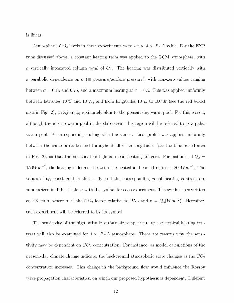
The high latitude surface warming is accompanied by stationary waves. The January

250-hPa geopotential height (δZ) field (Fig. 3b) shows a poleward propagating wave train

(see the arching solid arrow) which emanates from a subtropical high centered at (40o, 30oN).

Being to the northwest of the imposed heating, the location of the subtropical high conforms

to the Rossby wave response to a localized tropical heat source, as was shown by Gill (1980).

If the tropical heating is lowered to 75 Wm−2 (EXP4-75), the stationary wave amplitude

weakens (Fig. 3a), but the NH wave structure is similar to that of the EXP4-150 case.

If the heating is increased to 225 Wm−2 (EXP4-225), the wave amplifies and takes on a

structure which indicates that a poleward propagating wave from the subtropical high is

quickly refracted back toward the equator. This wave route is indicated by the arrow in

Fig. 3c. It can be seen that the high in the equatorward propagating wave is as strong as

the high in the poleward propagating wave. There is still evidence of poleward propagation

farther into the Arctic (dashed arrow), but it appears that most of the wave energy is

refracted toward the equator. As will be discussed later, these results suggest that increased

equatorward refraction for large values of Qo limit the extent to which the localized tropical

heating can warm the Arctic.

14

6 Attributes of surface-air warming

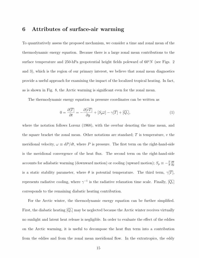
To quantitatively assess the proposed mechanism, we consider a time and zonal mean of the

thermodynamic energy equation. Because there is a large zonal mean contributions to the

surface temperature and 250-hPa geopotential height fields poleward of 60oN (see Figs. 2

and 3), which is the region of our primary interest, we believe that zonal mean diagnostics

provide a useful approach for examining the impact of the localized tropical heating. In fact,

as is shown in Fig. 8, the Arctic warming is significant even for the zonal mean.

The thermodynamic energy equation in pressure coordinates can be written as

0 =∂[T ]

∂t= −∂[vT ]

∂y+ [Spω]− γ[T ] + [Qr], (1)

where the notation follows Lorenz (1968), with the overbar denoting the time mean, and

the square bracket the zonal mean. Other notations are standard; T is temperature, v the

meridional velocity, ω ≡ dP/dt, where P is pressure. The first term on the right-hand-side

is the meridional convergence of the heat flux. The second term on the right-hand-side

accounts for adiabatic warming (downward motion) or cooling (upward motion); Sp ≡ −Tθ

∂θ∂p

is a static stability parameter, where θ is potential temperature. The third term, γ[T ],

represents radiative cooling, where γ−1 is the radiative relaxation time scale. Finally, [Qr]

corresponds to the remaining diabatic heating contribution.

For the Arctic winter, the thermodynamic energy equation can be further simplified.

First, the diabatic heating [Qr] may be neglected because the Arctic winter receives virtually

no sunlight and latent heat release is negligible. In order to evaluate the effect of the eddies

on the Arctic warming, it is useful to decompose the heat flux term into a contribution

from the eddies and from the zonal mean meridional flow. In the extratropics, the eddy

15

contribution is much greater (Pexioto and Oort 1992), and thus the zonal mean component

can be neglected. After making these assumptions, (1) can be re-written as

δ[T ] ≈ γ−1

(− ∂

∂yδ[v∗T

∗]− ∂

∂yδ[v′∗T ′∗] + δ[ωSp]

), (2)

where the asterisk denotes a deviation from the zonal mean, and the prime a deviation

from the time mean. The first term on the right-hand-side represents the meridional heat

flux convergence by the stationary eddies and the second term the meridional heat flux

convergence by the transient eddies. This equation states that Arctic warming will occur if

the sum of the heat flux convergence and adiabatic warming is positive in that region.

As was hypothesized, the eddy heat flux convergence is found to contribute to the NH

winter high latitude warming. Figure 4a shows that the change in the stationary eddy heat

flux convergence, caused by the localized tropical heating, warms the lowest model level

(σ = 0.993) across a broad zone extending from 17oN to 62oN . An exception is the narrow

latitudinal range centered at 40oN . This warming is compensated by cooling in the tropics,

and to a lesser extent by cooling poleward of 62oN . Between 48oN and 60oN , the warming

occurs at values ranging between ≈ 2× 10−6Ks−1 and ≈ 6× 10−6Ks−1. If γ = 30−1day−1,

(2) indicates that the warming caused by the stationary eddy heat flux at these latitudes

is between 5 K and 15 K. The temperature changes caused by these eddy heat fluxes are

comparable to the lowest model level δT (Fig. 1b).

The response of the transient eddies to the tropical heating (Fig. 4b) results in a low level

warming that is comparable to that by the stationary eddies, except that the transient eddy

warming is confined to a smaller range of latitudes and occurs farther poleward. Again if we

assume that γ = 30−1day−1, the warming caused by the transient eddy heat flux convergence

16

at these latitudes can reach 15 K. The sum of the stationary and transient eddy heat flux

convergences (Fig. 4c) shows that the strongest warming occurs between 50oN and 80oN .

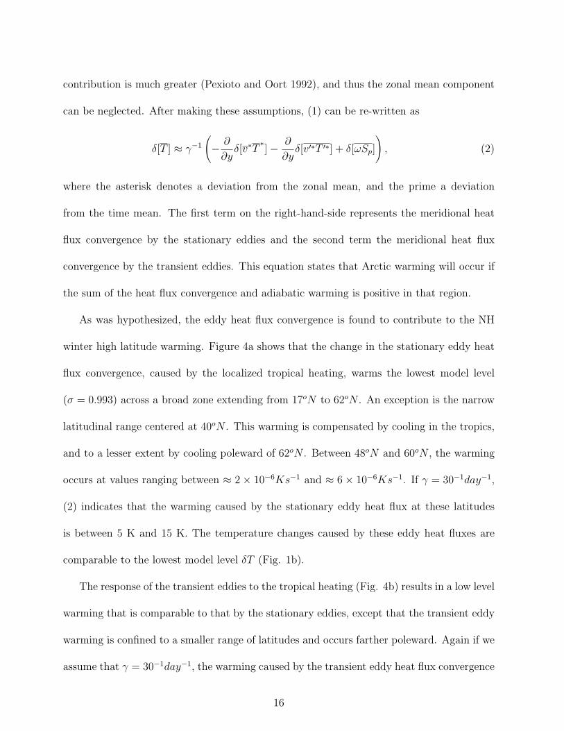
Poleward of 70oN , adiabatic warming plays a greater role in warming the surface. Figure

5a shows that between 70oN and 82oN , the anomalous adiabatic warming, δ[ωSp], accounts

for a surface warming of up to ≈ 5 × 10−6Ks−1. Once again assuming γ = 30−1day−1, the

resulting warming would be about 5K − 13K. This anomalous adiabatic warming (δ[ωSp])

can be explained mostly by changes in the (Sp[δω]) contribution, as can be inferred from δω

(Fig. 5b).

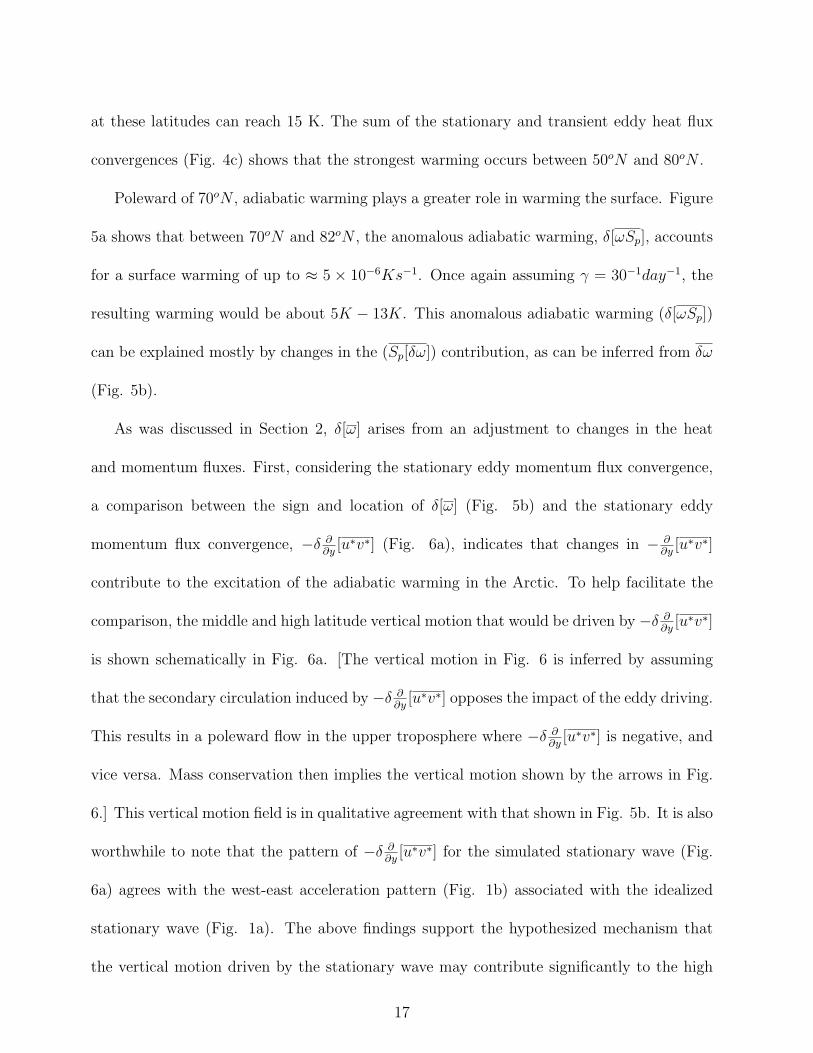
As was discussed in Section 2, δ[ω] arises from an adjustment to changes in the heat

and momentum fluxes. First, considering the stationary eddy momentum flux convergence,

a comparison between the sign and location of δ[ω] (Fig. 5b) and the stationary eddy

momentum flux convergence, −δ ∂∂y

[u∗v∗] (Fig. 6a), indicates that changes in − ∂∂y

[u∗v∗]

contribute to the excitation of the adiabatic warming in the Arctic. To help facilitate the

comparison, the middle and high latitude vertical motion that would be driven by −δ ∂∂y

[u∗v∗]

is shown schematically in Fig. 6a. [The vertical motion in Fig. 6 is inferred by assuming

that the secondary circulation induced by −δ ∂∂y

[u∗v∗] opposes the impact of the eddy driving.

This results in a poleward flow in the upper troposphere where −δ ∂∂y

[u∗v∗] is negative, and

vice versa. Mass conservation then implies the vertical motion shown by the arrows in Fig.

6.] This vertical motion field is in qualitative agreement with that shown in Fig. 5b. It is also

worthwhile to note that the pattern of −δ ∂∂y

[u∗v∗] for the simulated stationary wave (Fig.

6a) agrees with the west-east acceleration pattern (Fig. 1b) associated with the idealized

stationary wave (Fig. 1a). The above findings support the hypothesized mechanism that

the vertical motion driven by the stationary wave may contribute significantly to the high

17

latitude winter warming. In the Arctic where the adiabatic warming is taking place, the

impact of the transient eddy momentum flux convergence (Fig. 6b) is weaker than that of

the stationary eddy momentum flux convergence (Fig. 6a), and thus the sum of these two

convergences (Fig. 6c) would still drive downward motion.

The eddy heat flux also drives an overturning circulation, but because this portion of

the overturning circulation has a spatial structure that opposes the effect of the heat flux,

the eddy heat flux cannot indirectly contribute to adiabatic warming in the region between

70oN and 82oN . Therefore, we are led to conclude that the adiabatic warming over the

region ranging between 70oN and 82oN can be ascribed primarily to the stationary eddy

momentum flux convergence.

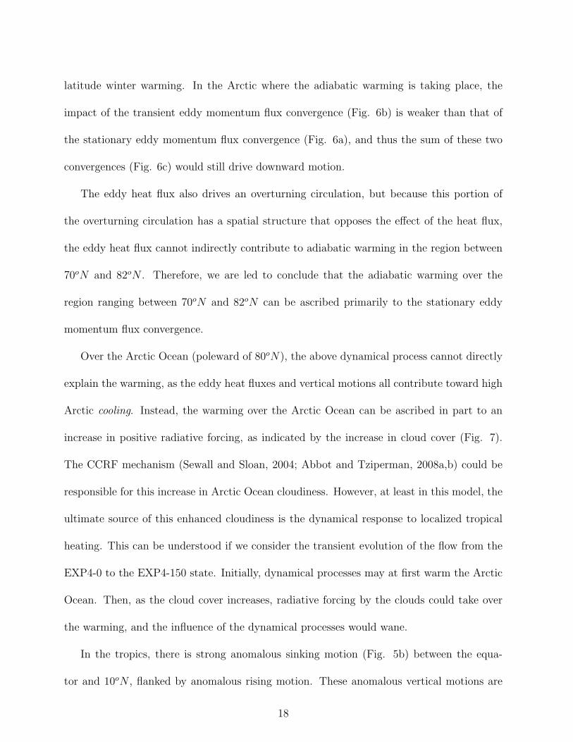
Over the Arctic Ocean (poleward of 80oN), the above dynamical process cannot directly

explain the warming, as the eddy heat fluxes and vertical motions all contribute toward high

Arctic cooling. Instead, the warming over the Arctic Ocean can be ascribed in part to an

increase in positive radiative forcing, as indicated by the increase in cloud cover (Fig. 7).

The CCRF mechanism (Sewall and Sloan, 2004; Abbot and Tziperman, 2008a,b) could be

responsible for this increase in Arctic Ocean cloudiness. However, at least in this model, the

ultimate source of this enhanced cloudiness is the dynamical response to localized tropical

heating. This can be understood if we consider the transient evolution of the flow from the

EXP4-0 to the EXP4-150 state. Initially, dynamical processes may at first warm the Arctic

Ocean. Then, as the cloud cover increases, radiative forcing by the clouds could take over

the warming, and the influence of the dynamical processes would wane.

In the tropics, there is strong anomalous sinking motion (Fig. 5b) between the equa-

tor and 10oN , flanked by anomalous rising motion. These anomalous vertical motions are

18

consistent with the thermal wind adjustment that would arise from the stationary Rossby

waves shown in Fig. 1. Although the sinking motion warms the lower troposphere (Fig. 5a),

the corresponding eddy heat flux divergence (Fig. 4a) cools the region. The cooling in the

tropics therefore can be interpreted as being a result of the poleward eddy heat flux (Fig.

2a).

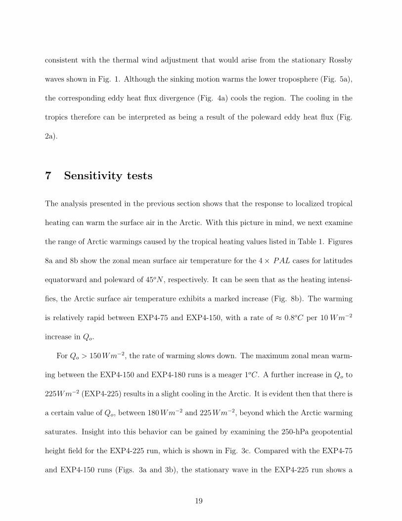
7 Sensitivity tests

The analysis presented in the previous section shows that the response to localized tropical

heating can warm the surface air in the Arctic. With this picture in mind, we next examine

the range of Arctic warmings caused by the tropical heating values listed in Table 1. Figures

8a and 8b show the zonal mean surface air temperature for the 4× PAL cases for latitudes

equatorward and poleward of 45oN , respectively. It can be seen that as the heating intensi-

fies, the Arctic surface air temperature exhibits a marked increase (Fig. 8b). The warming

is relatively rapid between EXP4-75 and EXP4-150, with a rate of ≈ 0.8oC per 10 Wm−2

increase in Qo.

For Qo > 150Wm−2, the rate of warming slows down. The maximum zonal mean warm-

ing between the EXP4-150 and EXP4-180 runs is a meager 1oC. A further increase in Qo to

225Wm−2 (EXP4-225) results in a slight cooling in the Arctic. It is evident then that there is

a certain value of Qo, between 180Wm−2 and 225Wm−2, beyond which the Arctic warming

saturates. Insight into this behavior can be gained by examining the 250-hPa geopotential

height field for the EXP4-225 run, which is shown in Fig. 3c. Compared with the EXP4-75

and EXP4-150 runs (Figs. 3a and 3b), the stationary wave in the EXP4-225 run shows a

19

more pronounced equatorward refraction in the NH midlatitudes, as highlighted by the solid

arrow. Presumably this refraction is caused by nonlinear wave dynamics because the wave

amplitude can be seen to increase with larger Qo. As the wave strengthens, nonlinear wave-

wave interactions are expected to become increasingly important. This is indeed supported

by the prominence of zonal wavenumber 3 and 4 features in Fig. 3c relative to Figs. 3a

and 3b; The ratio of the zonal to the meridional component of the stationary wave group

velocity vector is equal to k/l (James 1994), where k and l are the zonal and meridional wave

numbers, respectively. Therefore, as k increases, as is the case in Fig. 3, the propagation

to higher latitudes is expected to be suppressed, and instead the trajectory would acquire a

more zonal orientation.

Compared with the 4 × PAL EXP runs examined above, for 1 × PAL, intensifying

the tropical heating results in a weaker Arctic warming (Fig. 8d), with an average rate

of ≈ 0.3oC per 10 Wm−2 increase in Qo. This indicates that the impact of the localized

tropical heating on polar warming is dependent on the CO2 content of the atmosphere. This

sensitivity to the CO2 concentration could be caused by the difference in the background

state which can influence Rossby wave propagation characteristics (Grose and Hoskins 1979).

In addition, the CCRF and ice-albedo feedback mechanisms could also contribute to this

difference. By fixing the ice, snow, and clouds at their climatological values, the impact of

dynamical processes can be isolated from the CCRF and ice-albedo feedback mechanisms.

Similarly, by fixing the clouds, while allowing ice/snow to vary, the ice/snow-albedo feedback

can be isolated from the CCRF mechanism. However, as was discussed in Section 6, these

processes can be nonlinearly dependent on each other. For example, the ice-albedo effect,

which takes place during the warm season, may manifest itself during the following winter via

20

the CCRF feedback mechanism. This relationship between the summer ice-albedo feedback

and the winter CCRF can be tested with the second experiment mentioned above. However,

performing these experiments is beyond the scope of this study.

Saturation of the Arctic warming with respect to Qo also occurs for the 1× PAL EXP

runs, but compared with the 4× PAL EXP runs, the 1× PAL EXP runs show additional

complexity in that the EXP1-120 case exhibits a lower Arctic temperature than the EXP1-75

case (Fig. 8d). However, this is just one exception to the general relationship between the

Arctic surface warming and Qo.

With the results from the set of 1× PAL and 4× PAL experiments, we can ask what

are the relative impacts of quadrupling the CO2 content and strengthening the warm pool

heating on the Arctic surface air temperature. To address this question, using the results

from both the 1× PAL and 4× PAL runs, we subtract the surface air temperature from

the model runs with Q0 = 120 Wm−2, a value which corresponds to the warm pool heating

of the present-day climate, from model runs with Q0 = 150 Wm−2 and Q0 = 180 Wm−2,

plausible values of warm pool heating from the Cretaceous and early Cenozoic. We begin

by focusing on the impact of increasing Q0 while fixing the CO2 content at either 1× PAL

or 4 × PAL. As can be seen (Figs. 9d through 9g) the local temperature increases due to

these changes in Q0 can be as large as 6− 8oC. For the 4× PAL cases (Figs. 9d an 9e), the

most significant warming occurs over northern Siberia and the adjacent Arctic Ocean. For

the 1 × PAL cases (Figs. 9f and 9g), the strongest warming occurs near the present-day

Greenwich meridian, and the surface air temperature shows stronger zonal asymmetry than

the 4 × PAL cases. The differences between Figs. 9d and 9f and also Figs. 9e and 9g

also indicate that not only the zonal mean response but also the local response to increased

21

tropical heating is strongly influenced by the CO2 content of the model atmosphere.

The impact of quadrupling the CO2 content while fixing Q0 is shown in Fig. 9c. As can

be seen, the Arctic warming is much greater in Fig. 9c than in Figs. 9d through 9g especially

over the Arctic Ocean. This difference between the impact of the CO2 quadrupling and that

of the tropical heating is less marked over the northern Siberia where the localized tropical

heating accounts for a temperature increase of 4oC − 8oC, which corresponds to about 30%

of the warming associated with the CO2 quadrupling. The combined impact of quadrupling

the CO2 content and increasing Q0 is shown in Figs. 9a and 9b. The similarity in the two

temperature fields is consistent with Fig. 8b, which shows for this range of Q0 values that the

Arctic surface air temperature increase is close to saturation. Also, the larger temperatures

over northern Siberia in Figs. 9a and 9b, compared to Fig. 9c, further indicate that tropical

heating has an important influence in that region even in the presence of CO2 quadrupling.

Figures 8a and 8c show that the tropical surface air temperature slightly declines as Qo is

increased. The analysis of the thermodynamic energy budget presented in Section 6 indicates

that the localized tropical heating enhances the poleward heat transport which results in a

cooling of the tropics. Figures 9d through 9e all show that the strongest cooling occurs in

the vicinity of the imposed heating. This seems counter-intuitive, but it is important to

recall that in our experiment the heating is prescribed in order to mimic convective heating,

rather than heating at the surface. If our model had a warm pool, the tropical cooling would

be diminished because there would be a larger sensible heat flux from the ocean surface.

22

8 Concluding remarks and discussion

This study explores the hypothesis that localized tropical heating associated with a warm

pool can excite poleward propagating Rossby waves which can enhance the high latitude

warming associated with equable climates such as that of the Cretaceous and early Cenozoic.

For this purpose, we use an atmosphere-mixed layer ocean GCM with localized diabatic

heating over the deep tropics, along with compensating cooling at other longitudes. In order

to illustrate the workings of the hypothesized mechanism, we first contrasted two model

runs, one with this heating field and the other without, both with a 4× PAL CO2 content.

We find that the run with the heating produces substantially larger high-latitude surface air

temperatures.

Thermodynamic energy budget analysis was performed on the above two model runs.

This analysis shows that the high-latitude warming (excluding the region poleward of 82oN)

due to the localized tropical heating can be ascribed to eddy heat and momentum fluxes

associated with the Rossby waves forced by the tropical heating. In addition to the warming

by both stationary and transient eddy heat flux convergence, the eddy momentum flux also

contributes to the warming through its induction of sinking motion over high latitudes which

results in adiabatic warming. Farther poleward, over the Arctic Ocean, the warming driven

by the tropical heating coincides with an increase in cloud cover. Because solar radiation

does not reach the Arctic Ocean during the winter, we interpret this warming to have arisen

from radiative forcing which is enhanced by the increase in cloud cover. Our interpretation

is that the dynamical processes - meridional heat flux and adiabatic warming - first warm

the Arctic Ocean, hence increase the cloud cover. As the cloud cover increases, radiative

23

forcing by the clouds can take over the warming.

Setting aside for the moment the question of possible driving mechanisms for paleo

equable climates, from the perspective of improving our understanding the present-day cli-

mate, the role of warm pool convective heating on reducing the north-south temperature gra-

dient merits further discussion. Figure 8d shows that for a CO2 level of 1×PAL, the present-

day warm pool heating of 120Wm−2 causes the zonal mean winter Arctic surface air temper-

ature to rise by 3oC from that of a no-warm-pool climate. Therefore, our model calculations

suggest that without the tropical warm pool heating, the pole-to-equator difference in surface

temperature would be greater than is currently observed. A comparison with the correspond-

ing 4×PAL cases (Fig. 8b) suggests that as the atmospheric CO2 loading increases, localized

tropical heating becomes more effective in generating Arctic warming. It is also worth noting

that for the 4×PAL runs, the north-south temperature gradient reverses between 75oN and

the North Pole, if the tropical heating is greater than 120Wm−2 (Fig. 8b). This reversal in

the temperature gradient is reminiscent of the ‘Warm Arctic-Cold Continent’ teleconnection

pattern of the 2009-2010 winter (http://www.arctic.noaa.gov/reportcard/atmosphere.html).

Therefore, the ‘Warm Arctic-Cold Continent’ teleconnection pattern may strengthen as at-

mospheric CO2 loading increases and warm pool convective heating intensifies.

The effect of the localized tropical heating is limited though. For warm-pool heating

greater than 120Wm−2, there is a decline in the rate of Arctic warming with respect to

the heating intensity, and for heating greater than 180Wm−2 the Arctic warming halts

altogether. This saturation coincides with evidence of nonlinear processes whereby large

amplitude waves with higher zonal wave numbers refract equatorward. Thus, we interpret

the high latitude temperature saturation as arising from the suppression of wave propagation

24

into high latitudes.

To evaluate the extent to which an intensification of the warm pool convective heating can

contribute to the Arctic warming during the Cretaceous and early Cenozoic, we compared the

Arctic warming associated with 150 Wm−2 and 180 Wm−2 heating, possible values for that

time period, to that for a heating of 120Wm−2, a value which corresponds to the present-day

warm pool convective heating. Our model calculation finds an additional Arctic warming of

4oC − 8oC over northern Siberia and the adjacent Arctic Ocean. Relative to the warming

due to a quadrupling of CO2 alone, this temperature increase accounts for about 30% of the

warming over this region. As such, this finding suggests that local tropical heating is not

the major contributor to the winter Arctic warming. Nonetheless, warming of this amount

suggests that strengthened warm pool tropical convection may be an important contributor

to equable climate.

Although the above results suggest that the influence of localized tropical heating can

contribute to the high-latitude warming, it is important to keep in mind that there are

limitations to the model used in this study. For example, as far as we are aware, there

is no proxy evidence for a paleo warm pool in the Pacific, even though by analogy to the

present-day ocean circulation, it would not be surprising if there was indeed a warm pool

present during the Cretaceous and early Cenozoic. Furthermore, the value of the tropical

heating is uncertain, especially because reasonably accurate values of proxy SST in the

hypothesized warm pool are not known. Given these uncertainties, it is best to interpret our

findings as representing a plausible mechanism for increased high-latitude warming, with the

model temperatures representing possible range of values for high-latitude warming due to

enhanced warm pool convective heating.

25

Notwithstanding these shortcomings, our assumption of a paleo warm pool along with

localized diabatic heating appears to be consistent with the findings of Bush and Philander

(1997), who used a coupled atmosphere-ocean GCM to examine Cretaceous climate. Their

model findings indicate the presence of a warm pool along with enhanced precipitation that

spanned the longitudes from approximately 30oE to 90oE. In their study, the increase of

the model precipitation in this region was found to be about 25% greater than that outside

of the model warm pool.

Under the 4×PAL conditions, while the Arctic surface air temperature of the EXPm-n

(n 6= 0) runs is substantially higher than that of the corresponding EXPm-0 (m=1 or 4)

run, the differences in the overall tropospheric circulation pattern between the EXPm-0 and

EXPm-n runs are rather subtle. Perhaps the most notable feature is that as the localized

tropical heating intensifies, the upper tropospheric equatorial wind becomes less easterly

and eventually turns to westerly. This eastward acceleration is to be expected because the

imposed localized tropical heating generates Rossby waves, and as these waves emanate from

the tropics they transport eastward momentum into the equatorial region where the wave

source is located. Although this mechanism was not discussed by Bush and Philander (1997),

their Cretaceous run shows an upper tropospheric equatorial wind that is more westerly than

those for the present-day run. This feature is consistent with increased poleward Rossby wave

propagation out of the tropics.

Finally, it is worthwhile to note that the localization of the mid-tropospheric tropical

heating is compensated by dynamical cooling caused by the poleward eddy heat flux as-

sociated with the poleward propagating Rossby waves. If greenhouse gas warming causes

tropical convective heating to be more localized, as was discussed in Section 2, this mecha-

26

nism implies that the cooling caused by the eddy heat flux divergence may compensate for

greenhouse gas warming in the tropics. Therefore, in the face of increased greenhouse gas

loading, one may expect to find a muted warming in the tropics.

Acknowledgments:

For this study, the first author was supported by National Science Foundation Grant

ATM-0647776, and the second author by National Science Foundation Grant ATM-0649512.

The authors acknowledge Dr. Dorian S. Abbot for his helpful comments on an earlier version

of this manuscript.

27

References

[] Abbot, D.S. and E. Tziperman, 2008a: A high-latitude convective cloud feedback and

equable climates. Q. J. R. Meteorol. Soc. 134, 165-185.

[] Abbot, D.S. and E. Tziperman, 2008b: Sea ice, high-latitude convection, and equable

climates. Geophys. Res. Lett. 35, L03702, doi:10.1029/2007GL032286.

[] Allan, R. P., and B. J. Soden, 2008: Atmopsheric warming and the amplification of

precipitation extremes. Science, 321, 1481-1484. DOI: 10.1126/science.1160787

[] Barron, E.J., W.H. Peterson, D. Pollard and S.L. Thompson, 1993: Past climate and the

role of ocean heat transport: model simulations for the Cretaceous. Paleoceanography, 8,

785-798.

[] Barnston, A. G., and R. E. Livezey, 1987: Classification, seasonality, and persistence of

lowfrequency atmospheric circulation patterns. Mon. Wea. Rev., 115, 1083-1126.

[] Bice, K.L., D. Birgel, P./A. Meyers, K.A. Dahl, K.-U. Hinrichs and R.D. Norris, 2006: A

multiple proxy and model study of Cretaceous upper ocean temperatures and atmospheric

CO2 concentrations. Paleocean ogr., 21, PA2002, doi:10.1029/2005PA001203.

[] Bush, A. B., and S. G. H. Philander, 1997: The late Cretaceous: Simulations with a

coupled atmosphere-ocean general circulation model. Paleoceanography, 12, 495-516.

[] Charney, J. G., and P. G. Drazin, 1961: Propagation of planetary-scale disturbances from

the lower into the upper atmosphere. J. Geophys. Res., 66, 83-109.

28

[] DeConto, R.M., E.C. Brady, J.C. Bergengren and W.W. Hay, 2000: Late Cretaceous

climate, vegetation and ocean interactions in Warm Climates in Earth History, B. R.

Huber, K. G. MacLeod, S. L. Wing, Eds., Cambrige Univ. Press, pp. 275-296.

[] Emanuel, K., 2008: The hurricane-climate connection. Bull. Amer. Meteor. Soc., 89, 5,

ES10-ES20.

[] Farrell, B. F., 1990: Equable climate dynamics. J. Atmos. Sci. 47, 2986-2995.

[] Fletcher, B.J., S.J. Brentnall, C.W. Anderson, R.A. Berner and D. J. Beerling, 2008:

Atmospheric carbon dioxide linked with Mesozoic and early Cenozoic climate. Nature

Geoscience 1, 43-48.

[] Forster, A., Schouten, S., Baas, M., Sinninghe Damste, J., 2007: Mid-Cretaceous Albian-

Santonian sea surface temperature record of the tropical Atlantic Ocean, Geology, 35(10),

919-922.

[] Gill, A. E., 1980: Some simple solutions for heat-induced tropical circulation. Quart. J.

Roy. Meteor. Soc., 106, 447-462.

[] Held, I.M., 1975: Momentum transport by quasi-geostrophic eddies. J. Atmos. Sci. 32,

1494-1497.

[] Held, I.M. and Soden, B.J., 2006: Robust repsonses of the hydrological cycle to global

warming. J. Climate 19, 5686-5699.

[] Holton, J. R., 2004: An Introduction to Dynamic Meteorology. Academic Press, , 535 pp.

535 pp.

29

[] Horel, J. D. and J. M. Wallace, 1981: Planetary-Scale Atmospheric Phenomena Associated

with the Southern Oscillation. Mon. Wea. Rev., 109 , 813–829.

[] Huber, M., 2008: A hotter greenhouse? Science 321, 353-354.

[] Hunter, S. J., P. J. Valdes, A.M. Haywood and P. J. Markwick, 2008: Modelling Maas-

trichtian climate: investigating the role of geography, atmospheric CO2 and vegetation.

Clim. Past Discuss., 4, 981-1019.

[] James, I. N., 1995: Introduction to Circulating Atmospheres. Cambridge University Press,

448 pp.

[] Johnson, N. C. and S. B. Feldstein, 2009: The continuum of North Pacific sea level

pressure patterns: Intraseasonal, interannual and interdecadal variability. J. Climate, , in

press.

[] Kirk-Davidoff, D.B., P. Schrag and J.G. Anderson, 2002: On the feedback of stratospheric

clouds on polar climate. Geophys. Res. Lett., 29, 11, 1556, doi: 10.1029/2002GL014659.

[] Korty, R.L., K.A. Emanuel and J.R. Scott, 2008: Tropical cyclone-induced upper-ocean

mixing and climate: Application to equable climates. J. Climate, 21, 638-654.

[] Kumar, A., B. Jha, and M. L’Heureux, 2010: Are tropical SST trends chang-

ing the global teleconnection during La Nina? Geophy. Res. Lett., 37, L12702,

doi:10.1029/2010GL043394.

[] Kump, L.R. and D. Pollard, 2008: Amplification of Cretaceous warmth by biological cloud

feedbacks. Science, 320, 195.

30

[] Lin, J.-L., G. N. Kiladis, B. E. Mapes, K. M. Weickmann, K. R. Sperber, W. Lin, M.

C. Wheeler, S. D. Schubert, A. Del Genio, L. J. Donner, S. Emori, J.0F. Gueremy, F.

Hourdin, Ph. J. Rasch, E. Roeckner, and J. F. Scinocca, 2006: Tropical intraseasonal

variability in 14 IPCC AR4 climate models. Part I: convective signals. J. Climate, 19,

2665-2690.

[] Matthews, A. J., B. J. Hoskins and M. Mastuni, 2004: The Global Response to Tropical

Heating in the Madden-Julian Oscillation during Northern Winter. Q. J. R. Meteorol.

Soc., 130, 1991–2011.

[] Mori, M., and M. Watanabe, 2008: The growth and triggering mechanism of the PNA: a

MJO-PNA coherence. J. Meteor. Soc. Japan, 86, 213-236.

[] Otto-Bliesner, B.L. and G.R. Upchurch, 1997: Vegetation-induced warming of high-

latitude regions during the late Cretaceous period. Nature, 385, 804-807.

[] Otto-Bliesner, B.L., E.C. Brady and C. Shields, 2002: Late Cretaceous ocean: Coupled

simulations with the National Center for Atmospheric Research Climate System Model.

J. Geophys. Res., 107, D2, 4019, doi: 10.1029/2001JD000821.

[] Peixoto, J. P. and A. H. Oort, 1992: Physics of Climate. American Institute of Physics, ,

520 pp.

[] Poulsen, C. J., Pollard, D. and White, T. S., 2007: General Circulation Model simulation

of the d18O content of continental precipitation in the middle Cretaceous: A model-proxy

comparison. Geology, 35, 199-202.

31

[] Schubert, S. D. and C.-K. Park, 1995: Low-Frequency Intraseasonal Tropical-

Extratropical Interactions. J. Atmos. Sci., 48, 629-650.

[] Sewall, J.O. and L.C. Sloan, 2004: Arctic Ocean and reduced obliquity on early Paleogene

climate. Geology, 32, 477-480.

[] Sloan, L.C. and D. Pollard, 1998: Polar stratospheric clouds: a high latitude warming

mechanism in an ancient greenhouse world. Geophys. Res. Lett., 25, 3517-3520.

[] Sloan, L. C., J.C.G. Walker and T.C. Moore, 1995: The role of oceanic heat transport in

early Eocene climate. Paleoceanography, 10, 347-356.

[] Sloan, L.C., M. Huber and A. Ewing, 1999: Polar stratospheric cloud forcing in a green-

house world. In: Reconstructing Ocean History: A Window into the Future, eds. Abrantes

and Mix, Kluwer Academic/Plenum Publ., 273-293.

[] Spicer, R.A., A. Ahlberg., A.B. Herman, C.-C. Hofmann, M. Raikevich, P.J. Valdes and

P.J. Markwick, 2008: The Late Cretaceous continental interior of Siberia: A challenge for

climate models. Earth Plan. Sci. Lett., 267, 228-235.

[] Sriver, R.L. and M. Huber, 2007: Observational evidence for an ocean heat pump induced

by tropical cyclones. Nature, 447, 577-580.

[] Thompson, S.L. and D. Pollard, 1997: Greenland and Antarctic mass balances for present

and doubled CO2 from the GENESIS version 2 global: climate model. J. Climate, 10,

871-900.

32

[] Trenberth, K. E., and J. M. Caron, 2001: Estimates of meridional atmoshere and ocean

heat transports. J. Climate, 14, 3433-3443.

[] Wallace, J. M., and D. S. Gutzler, 1981: Teleconnections in the geopotential height field

during the Northern Hemisphere winter. Mon. Wea. Rev., 109, 784-804.

[] Wunsch, C., 2005: The total meridional heat flux and the oceanic and atmospheric parti-

tion. J. Climate, 18, 4374-4380.

[] Zhou, J., C.J. Poulsen, D. Pollard and T.S. White, 2008: Simulation of modern and

middle Cretaceous marine d18O with an ocean-atmosphere general circulation model.

Paleoceanography, 23, PA3223, doi:10.1029/2008PA001596, 1-11.

33

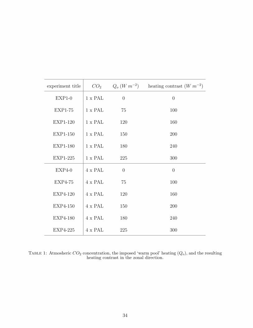
experiment title CO2 Qo (W m−2) heating contrast (W m−2)

EXP1-0 1 x PAL 0 0

EXP1-75 1 x PAL 75 100

EXP1-120 1 x PAL 120 160

EXP1-150 1 x PAL 150 200

EXP1-180 1 x PAL 180 240

EXP1-225 1 x PAL 225 300

EXP4-0 4 x PAL 0 0

EXP4-75 4 x PAL 75 100

EXP4-120 4 x PAL 120 160

EXP4-150 4 x PAL 150 200

EXP4-180 4 x PAL 180 240

EXP4-225 4 x PAL 225 300

Table 1: Atmosheric CO2 concentration, the imposed ‘warm pool’ heating (Qo), and the resultingheating contrast in the zonal direction.

34

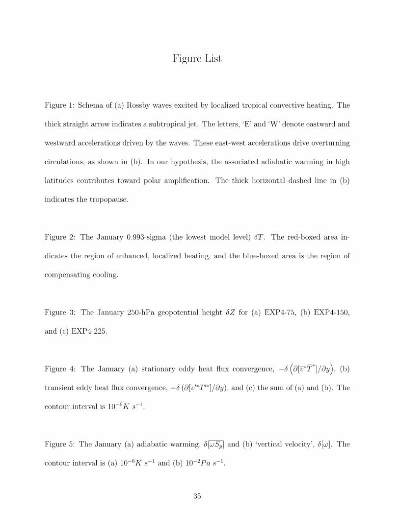
Figure List

Figure 1: Schema of (a) Rossby waves excited by localized tropical convective heating. The

thick straight arrow indicates a subtropical jet. The letters, ‘E’ and ‘W’ denote eastward and

westward accelerations driven by the waves. These east-west accelerations drive overturning

circulations, as shown in (b). In our hypothesis, the associated adiabatic warming in high

latitudes contributes toward polar amplification. The thick horizontal dashed line in (b)

indicates the tropopause.

Figure 2: The January 0.993-sigma (the lowest model level) δT . The red-boxed area in-

dicates the region of enhanced, localized heating, and the blue-boxed area is the region of

compensating cooling.

Figure 3: The January 250-hPa geopotential height δZ for (a) EXP4-75, (b) EXP4-150,

and (c) EXP4-225.

Figure 4: The January (a) stationary eddy heat flux convergence, −δ(∂[v∗T

∗]/∂y

), (b)

transient eddy heat flux convergence, −δ (∂[v′∗T ′∗]/∂y), and (c) the sum of (a) and (b). The

contour interval is 10−6K s−1.

Figure 5: The January (a) adiabatic warming, δ[ωSp] and (b) ‘vertical velocity’, δ[ω]. The

contour interval is (a) 10−6K s−1 and (b) 10−2Pa s−1.

35

Figure 6: The January (a) stationary eddy momentum flux convergence, −δ (∂[u∗v∗]/∂y),

(b) transient eddy momentum flux convergence, −δ(∂[u′∗v′

∗]/∂y

), and (c) the sum of (a)

and (b). The contour interval is 10−5m s−2. The arrows in (a) and (c) indicates high-latitude

overturning circulations induced by the corresponding momentum flux convergence. No ar-

rows are drawn in (b) because the momentum flux convergence structure is too complex to

readily infer the vertical motion.

Figure 7: The January total cloud cover fraction difference.

Figure 8: The January zonal mean surface air temperature for 4 × PAL CO2 cases; (a)

and (b) respectively show the temperature in the interval between the equator and 45oN ,

and 45oN and 90oN . In a similar manner, (c) and (d) shows the January zonal mean surface

air temperature for 4× PAL CO2 cases.

Figure 9: The January surface temperature difference amongst various experiment runs.

For each panel, the experiment runs used to produce the difference field are indicated on top

of the panel.

36

pole

east

westequator

E

E

W

W

(a)

east

height

E W E W

(b)

Adiaba/cwarming

equator pole

Figure 1: Schema of (a) Rossby waves excited by localized tropical convective heating. The thickstraight arrow indicates a subtropical jet. The letters, ‘E’ and ‘W’ denote eastward and westwardaccelerations driven by the waves. These east-west accelerations drive overturning circulations, asshown in (b). In our hypothesis, the associated adiabatic warming in high latitudes contributes

toward polar amplification. The thick horizontal dashed line in (b) indicates the tropopause.

37

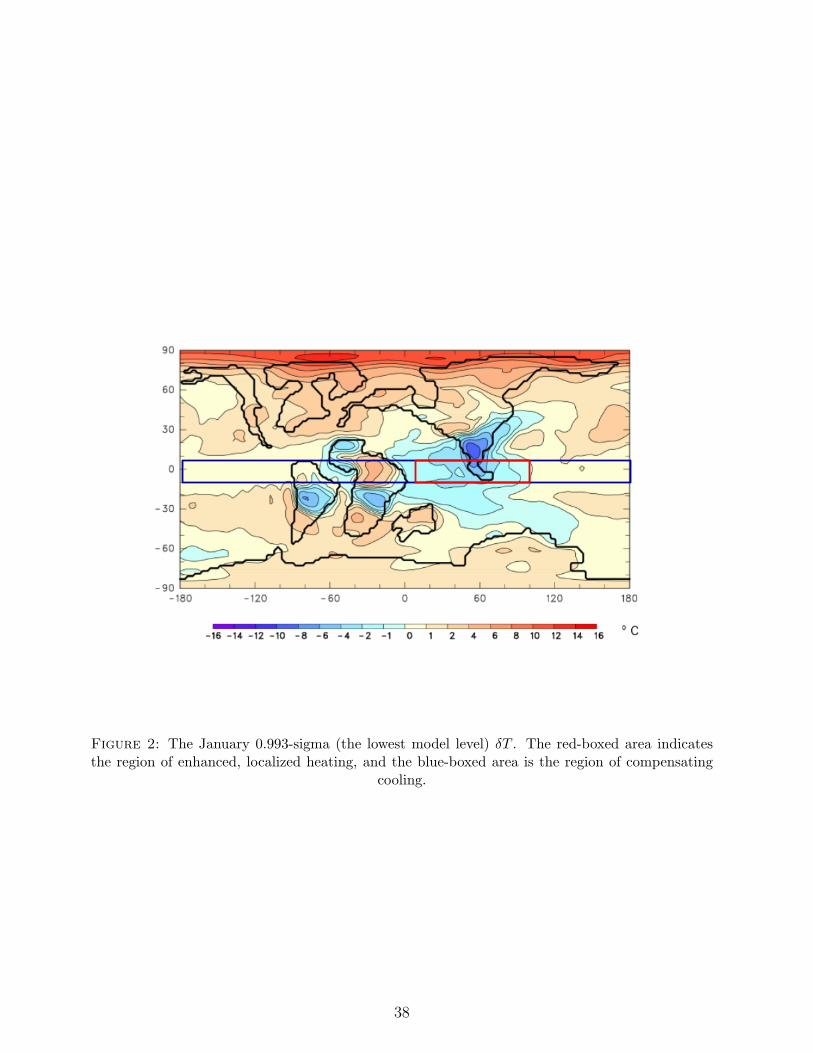
Figure 2: The January 0.993-sigma (the lowest model level) δT . The red-boxed area indicatesthe region of enhanced, localized heating, and the blue-boxed area is the region of compensating

cooling.

38

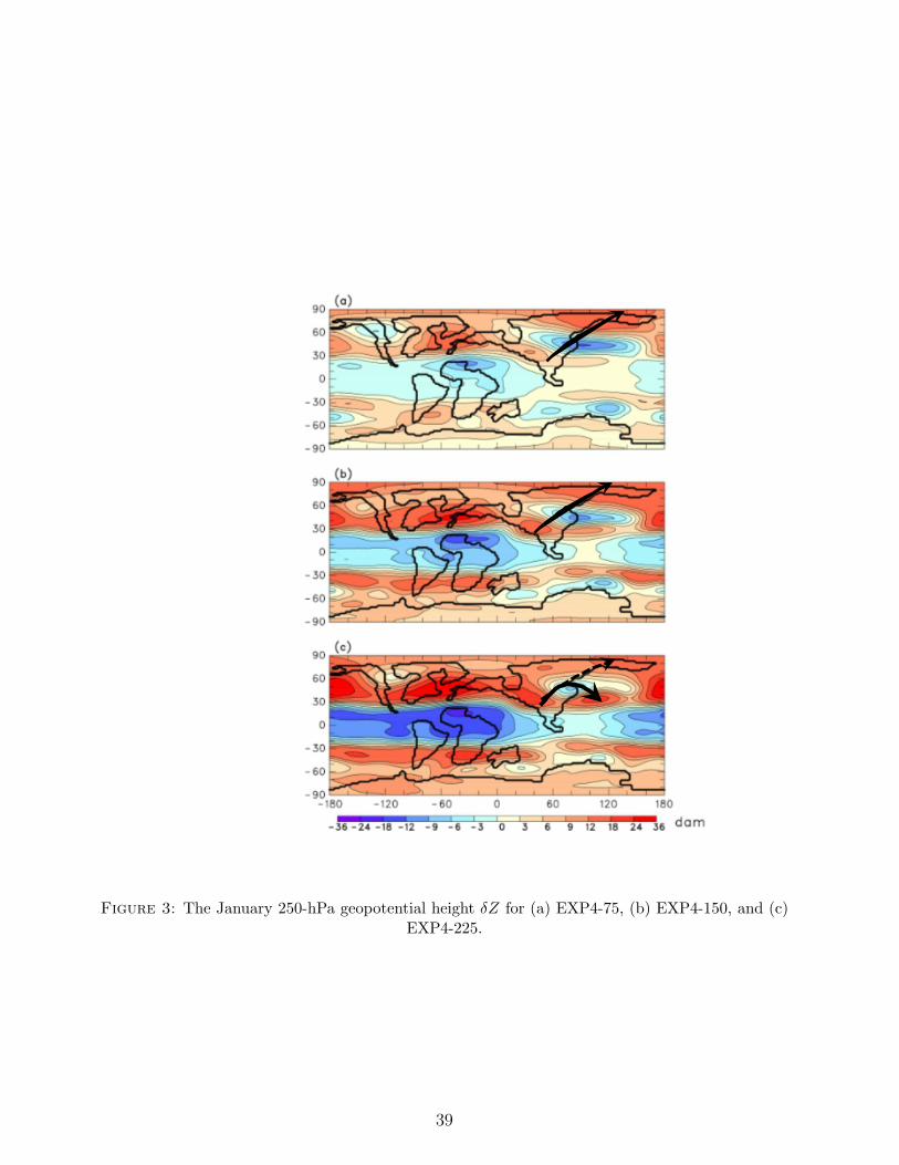
Figure 3: The January 250-hPa geopotential height δZ for (a) EXP4-75, (b) EXP4-150, and (c)EXP4-225.

39

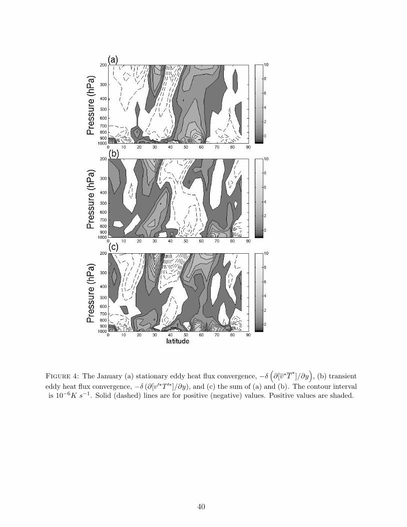
Figure 4: The January (a) stationary eddy heat flux convergence, −δ(∂[v∗T ∗]/∂y

), (b) transient

eddy heat flux convergence, −δ (∂[v′∗T ′∗]/∂y), and (c) the sum of (a) and (b). The contour intervalis 10−6K s−1. Solid (dashed) lines are for positive (negative) values. Positive values are shaded.

40

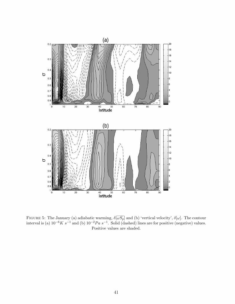
Figure 5: The January (a) adiabatic warming, δ[ωSp] and (b) ‘vertical velocity’, δ[ω]. The contourinterval is (a) 10−6K s−1 and (b) 10−2Pa s−1. Solid (dashed) lines are for positive (negative) values.

Positive values are shaded.

41

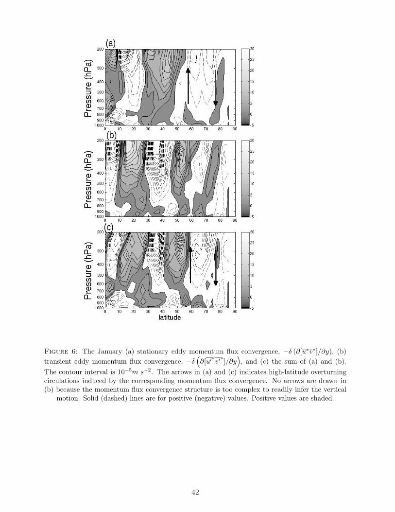
Figure 6: The January (a) stationary eddy momentum flux convergence, −δ (∂[u∗v∗]/∂y), (b)transient eddy momentum flux convergence, −δ

(∂[u′∗v′∗]/∂y

), and (c) the sum of (a) and (b).

The contour interval is 10−5m s−2. The arrows in (a) and (c) indicates high-latitude overturningcirculations induced by the corresponding momentum flux convergence. No arrows are drawn in(b) because the momentum flux convergence structure is too complex to readily infer the vertical

motion. Solid (dashed) lines are for positive (negative) values. Positive values are shaded.

42

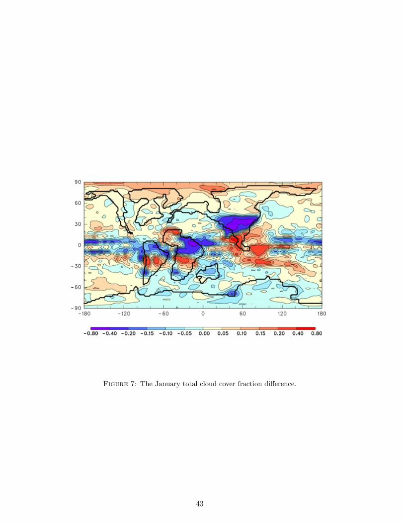
Figure 7: The January total cloud cover fraction difference.

43

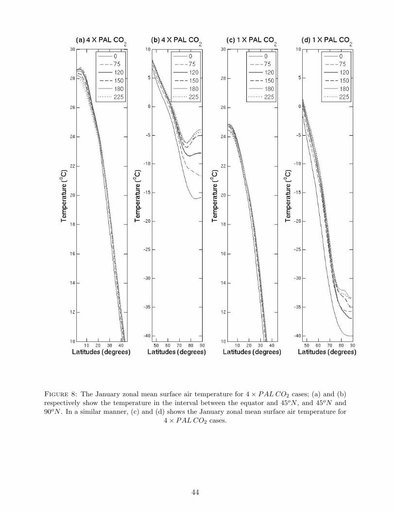
Figure 8: The January zonal mean surface air temperature for 4 × PAL CO2 cases; (a) and (b)respectively show the temperature in the interval between the equator and 45oN , and 45oN and90oN . In a similar manner, (c) and (d) shows the January zonal mean surface air temperature for

4× PAL CO2 cases.

44

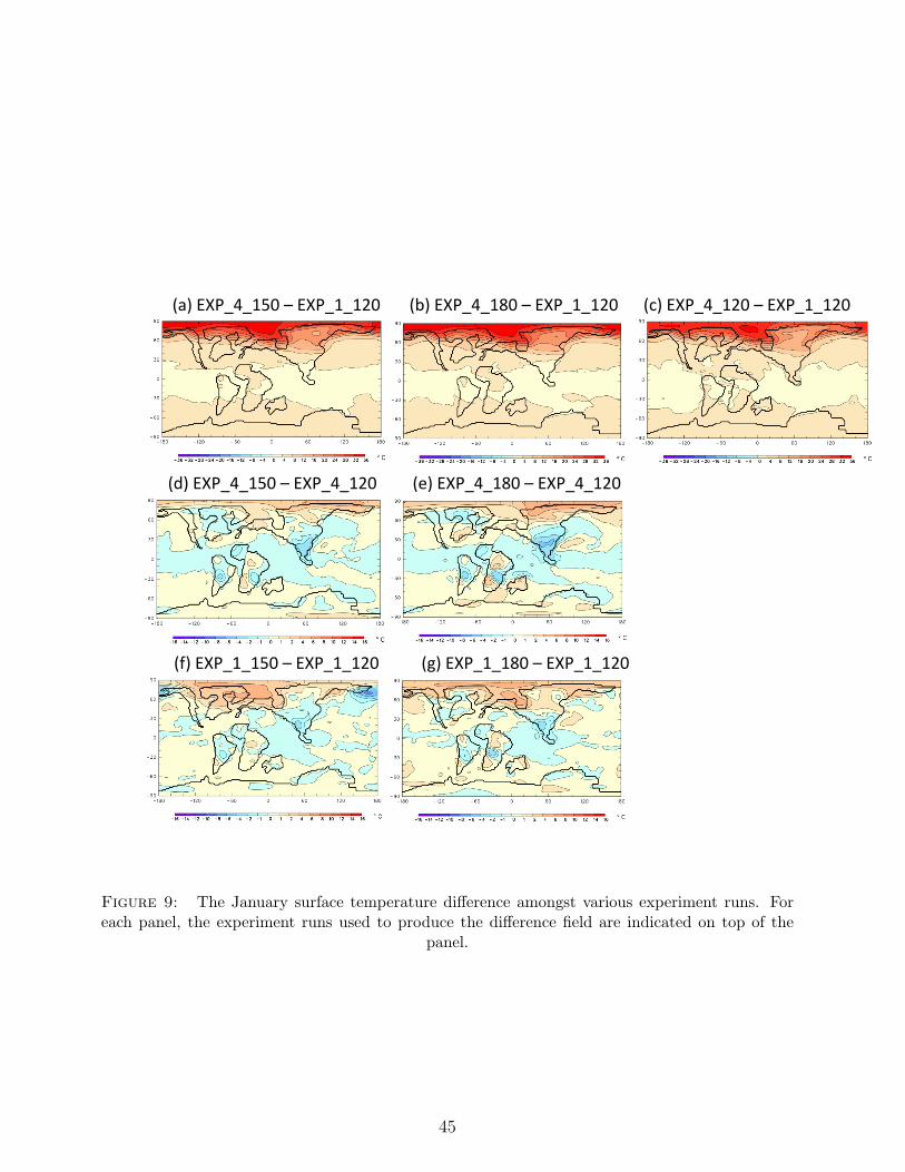
(a)EXP_4_150–EXP_1_120 (b)EXP_4_180–EXP_1_120 (c)EXP_4_120–EXP_1_120

(f)EXP_1_150–EXP_1_120 (g)EXP_1_180–EXP_1_120

(d)EXP_4_150–EXP_4_120 (e)EXP_4_180–EXP_4_120

Figure 9: The January surface temperature difference amongst various experiment runs. Foreach panel, the experiment runs used to produce the difference field are indicated on top of the

panel.

45