Embed Size (px)
Citation preview
1
Do Reorganization Costs Matter for Efficiency? Evidence from a Bankruptcy Reform in Colombia
Xavier Giné and Inessa Love*
July 2008
Abstract
An efficient bankruptcy system should liquidate unviable businesses and reorganize viable ones. The importance of this “filtering” process has long been recognized in the literature, yet the typical reason advanced for its failure has been biases (in codes or among judges). In this paper we show that bankruptcy costs can be another source of such filtering failure. We illustrate this with the Colombian reform of 1999. Using data from 1,924 firms filing for bankruptcy between 1996 and 2003, we find that the pre-reform reorganization proceedings were so inefficient that the bankruptcy system failed to separate economically viable firms from inefficient ones. In contrast, by streamlining the reorganization process, the reform improved the selection of viable firms into reorganization. In this sense, the new law increased the efficiency of the bankruptcy system in Colombia.
JEL: G33 G34 Keywords: bankruptcy reform, reorganization, liquidation, Colombia
_____________________________________________
* Emails: [email protected] and [email protected]. Both authors are affiliated with the World Bank, 1818 H Street, Washington, DC 20433. We wish to thank Fernando Montes-Negret for sparking our interest in this topic, Enrique Aguirre and the Superintendencia de Sociedades for the data and Rodolfo Danies Lacouture, the Superintendent, for insightful comments on an earlier draft. We also wish to thank Jaime Alberto Gomez, Jorge Pinzón, Adolfo Rouillon, Felipe Trias and Carlos Urrutia for very useful conversations about the intricacies of the bankruptcy law in Colombia. We finally wish to thank Rei Odawara for excellent research assistance and to Jishnu Das, Asli Demirguc-Kunt, Quy-Toan Do, Leora Klapper, Soledad Martínez Peria, Claudio Raddatz and Kenichi Ueda for valuable comments.
I. Introduction
Nearly ninety countries around the world have reformed their bankruptcy codes since
World War II and over half of them have done so during the last decade. The extent to
which these reforms will improve efficiency depends on their design and the context in
which the new codes are binding (Claessens et al., 2001; Franks and Loranth, 2005; Hart,
2000; Djankov et al., 2006 and World Bank, 2004, 2005 and 2006). A key aspect of an
efficient bankruptcy system is its ability to encourage the reorganization of viable firms
and the liquidation of unviable ones. This requires a delicate balance (White, 1989). On
the one hand, if the law is lenient towards failing firms, it will inevitably allow inefficient
firms to continue operations. On the other, if the law favors liquidation, it will also
liquidate viable firms.
Due to this trade-off, the design of bankruptcy laws is still a much debated topic
(Claessens and Klapper, 2003; Smith and Strömberg, 2004 and references therein). The
debate has focused on comparing two stylized bankruptcy proceedings: cash auctions or
liquidations and structured bargainings or reorganizations. Critics of reorganizations
argue that conflicting interests among claimholders and managers lead to excessively
lengthy and costly negotiations (Baird, 1986; Aghion et al., 1992). Critics of liquidations
claim that they contribute to the inefficient sale of assets due to market illiquidity and
transaction costs (Shleifer and Vishny, 1992; Aghion et al., 1992).1
While there is a growing literature estimating the costs of bankruptcy (see Bris et
al. 2006 for a review), there is little empirical evidence assessing how these costs affect
the ability of the bankruptcy system to separate viable businesses from unviable ones, a
key to ensuring efficiency. This paper attempts to fill this gap by using a bankruptcy
reform that took place in Colombia.
In the midst of financial crisis, facing a backlog of failing businesses entering a
very inefficient bankruptcy process, Colombia adopted a new reorganization code in late
1999. This law, known as Law 550, streamlined the reorganization process by
establishing shorter statutory deadlines for reorganization plans, reducing opportunities
for excessive appeals by debtors (who typically delayed the process in order to suspend
1 Using data from Sweden, Stromberg (2000) show that liquidations also suffer from conflicts of interest among claimholders.
2
the debt service) and requiring mandatory liquidation in cases of failed negotiations.
The Colombian reform can be seen as a natural experiment with two regimes: a
pre-reform regime with high reorganization costs and the post-reform regime with low
costs. In a regime with high costs, some viable businesses may be liquidated if the costs
they face are too high. In this case, the bankruptcy system fails to separate viable from
unviable firms, resulting in inefficient outcomes. In contrast, when reorganization costs
are low, better quality firms are more likely to choose reorganization, resulting in a clear
separation between firms that reorganize and those that liquidate. In this regime, as a
result of both lower costs and better selection, the recovery after reorganization is faster.
Our focus on ex-post efficiency stems from the fact that in Colombia, as in most
countries, ex-ante contract clauses specifying how to deal with insolvency events would
be superseded by the provisions of the insolvency law upon filing for bankruptcy. It is not
surprising then that these contracts are seldom written.2
We use a unique dataset obtained from the Colombian Superintendence of
Companies which includes a total of 1,924 bankruptcy cases, representing the universe of
cases filed between 1996 and 2004, conveniently spanning the reform episode. We also
use data of about 14,000 active companies that report to the same Superintendence over
the same time period. The dataset predominantly consists of non-listed firms thus
complementing the US literature, which has focused mainly on public firms.3 We use
data from financial statements and accounting-based models (e.g. Z-score model of
Altman 1968 and 2000) to construct an indicator of financial distress.
We show that the reform made reorganization an attractive option for distressed
but viable firms. First, we confirm that in accordance with the text of the reform, the
duration of reorganization proceedings significantly decreased overall and also relative to
the duration of liquidations. While data on the direct costs of reorganization do not exist
in Colombia, this finding is in line with our hypothesis of lower costs after the reform,
2 See Adler (1997) and Schwartz (1997) for papers arguing for allowing such contracts. 3 The literature on reorganization costs in the US mostly draws conclusions from the relatively small number of public corporations (see for example Altman, 1984; Weiss, 1990 and Weiss and Wruck, 1998). Notable exceptions are Bris et al. (2005), which use a sample of 286 public and private firms and Morrison (2007a), who uses a sample of 95 small businesses. Davydenko and Franks (2005) use a large sample of small firms from France, Germany and the UK.
3
since the length of the process is likely to be a major indirect cost of the reorganization
process. Second, under the old law, we observe that firms filing for reorganization are
indistinguishable from those filing for liquidation based on several measures of financial
health. In contrast, relatively weaker (and hence less viable) firms are more likely to file
for liquidation after the new law, resulting in a clear separation in the distribution of the
two types of firms. Finally, we find that the level of recovery after the reorganization
episode is significantly improved under the new law. While under the old law firms
hovered at about the same low level of financial health for years after entering into
reorganization, we observe a clear recovery under the new law. We conclude that the new
law increased the efficiency of the bankruptcy system in Colombia.
Previous bankruptcy studies analyze the existing laws of a given country or make
comparisons across different countries. Evidence from the US Chapter 11 reorganizations
offers mixed conclusions on the magnitude of these costs. While Altman (1984) and
Hotchkiss (1995) among others find high Chapter 11 costs, Alderson and Betker (1995)
and Maksimovic and Phillips (1998) find them to be low. More recently, Morrison
(2007a) also finds that contrary to what is commonly thought, Chapter 11 filings among
small businesses are relatively cheap and exhibit little bias. Bris et al. (2006) show that
reorganization costs are heterogeneous across firms but comparable to US Chapter 7
liquidations costs, although reorganizations as compared to liquidations preserve the
assets better. In contrast, Thorburn (2000) finds that liquidations in Sweden, which have a
statutory deadline, are faster and cheaper than reorganizations in the US. Bris et al.
(2006), however, question the validity of the comparison, because the US and Sweden
differ from each other in many other ways besides the bankruptcy codes.
In this paper, we look at the impact of a more streamlined procedure that includes
a statutory deadline in the reorganization proceeding but avoid country comparisons by
studying a bankruptcy reform within a single country. We exploit the fact that the reform
only changed the reorganization proceeding, allowing us to compare the pool of firms
that file for reorganization to the pool of firms filing for liquidation before and after the
law. However, since the law was introduced because of a major financial crisis, we need
to make sure that we can attribute the effects to the new law and not the changing
4
macroeconomic conditions.4 To do that we create a sample of matching active firms
(matched to filing firms by size, industry and year) and contrast filing firms with active
firms. We also control for the overall trend that captures any potential gradual
improvement of the judicial system and test robustness of our results by explicitly
controlling for crisis years and by removing the crisis window from the sample. We find
that while the crisis negatively affected the financial health of all firms in Colombia,
there was no differential effect of the crisis on filing firms relative to active firms and on
firms filing for reorganization relative to those filing for liquidation. This evidence
supports our identification strategy.
The rest of the paper is organized as follows. Section II outlines the main
hypothesis to be tested, while Sections III and IV present and describe the data in detail.
Section V presents our empirical specifications and main results and Section VI presents
the robustness tests. Section VII concludes. The background information on the
bankruptcy system in Colombia and details of the reorganization Law 550 of 1999 are
presented in Appendix 1.
II. Testable Hypotheses
This section describes the testable hypotheses that follow from the introduction of
the new law, which shortened the reorganization process by limiting the amount of time it
takes to approve the reorganization plan, streamlined the process and reduced debtor’s
power to derail and slow down the process. The hypotheses are as follows: (A) reduction
in reorganization time, (B) selection of healthier firms into reorganization, and (C) faster
recovery of reorganized firms.5
A. Duration of Reorganization
We interpret part of the effect of Law 550 as a decline in reorganization costs.
4 See Uribe and Vargas (2002) or Urrutia and Zárate (2001) for details about the causes and magnitude of the crisis. 5 Gine and Love (2006) presents a model that elaborates these hypotheses more formally. In addition, the model provides intuition about the role that bankruptcy costs play in determining the ability of the system to filter viable from non-viable firms.
5
One obvious component of the overall cost of reorganization is the time it takes to
approve the reorganization plan (Franks and Torous, 1989 or more recently Bris et al.,
2006). Higher involvement in the process takes managers’ time away from actually
running the firm, which adds to the costs. Likewise, a prime direct cost is lawyer’s fees,
and so the shorter the proceedings and the less lawyer involvement in a more streamlined
process, the lower the expenses should be. Since the new law limited the negotiations to a
maximum of eight months, one would expect total costs (direct and indirect) to also
decrease on average. As already mentioned, because we do not have data on direct costs,
we use the length of the process as a proxy for this overall cost.
Hypothesis A1. The duration of reorganization decreases after the new law is
introduced (overall and relative to liquidations).
Since we use duration as a proxy for costs, we test this assumption by using
indirect liquidation costs (measured by the duration of liquidations) as a proxy for
liquidation value: 6
Hypothesis A2. The duration of liquidation remains constant after the new law.
This hypothesis is also important because, if confirmed, it allows us to make sure
that the reorganization results are not driven by the overall improvement in the
Colombian judicial system. To test the validity of these hypotheses, we compare the
length of reorganization and liquidation cases before and after the law.
B. Selection into Reorganization
Our main hypothesis is that the reform contributed to the efficiency of the
bankruptcy law by separating viable from non viable firms. If the reorganization process
is inefficient, it will fail to separate viable from unviable firms. Here we test whether the
6 Liquidation values could also be driven by the fluctuations in the scrap value of the assets that are uncorrelated with the costs of liquidation as measured by the length of the process. We don’t have adequate data to test this assumption.
6
new Law 550 improved the efficiency of the bankruptcy system by encouraging viable
firms to choose reorganization as a now attractive alternative, while non-viable firms go
into liquidation.
Hypothesis B1. Before the new law, liquidating firms are on average
indistinguishable from reorganizing firms, while after the law, liquidating firms have
weaker financial health, on average, relative to reorganizing firms.
In addition, if Hypothesis B1 is true, that is if reorganizing firms are relatively
healthier than liquidating firms after the reform, the number of reorganization cases that
end up in mandatory liquidations should be lower.
Hypothesis B2. The number of reorganizations that result in mandatory
liquidation is lower after the new law.
C. Recovery after Reorganization
As a direct result of both lower costs and better selection, the recovery of
distressed firms after reorganization should improve significantly.
Hypothesis C. Reorganized firms recover faster after the new law.
There is reason to believe that by reducing the bankruptcy costs and reducing the
discretion of owners and managers, the reform may have altered the bargaining power of
managers vis à vis creditors. After the reform, the reorganization provisions became less
costly to creditors and less beneficial to managers, thus redistributing bargaining power
between the two groups (see, for example, Baird and Picker, 1991). We unfortunately
lack the data to assess how this redistribution took place.7
7 We thank the referee for alerting us to this fact. It seems likely that before the reform, nonviable businesses used the law to impose delay on their creditors. This way managers could keep their jobs for at least a little longer or they could gamble on the firm's resurrection. After the reform, this option is less attractive, although there is evidence suggesting that the new law was still favorable to debtors (see Tamayo et al. 2002 and Rouillon, 2006 for a discussion on this topic).
7
III. Data
The data used come from the Superintendence of Companies of Colombia. We
use two different datasets, bankruptcy filings and financial statements.
A. Bankruptcy Data
These data include the universe of liquidations (L) and reorganizations (R) filed
with the Superintendence from 1995 until 2004. Before 2000 (under Law 222), the
reorganization process was referred to as a Concordato (concordat), while after 2000
(under the Law 550), it was referred to as an Acuerdo (agreement).
All cases report the starting date but only about half report the ending date. Many
of the ending dates are missing because the process is still ongoing, especially among
liquidations. For firms that have a start and end of the filing, we construct a DURATION
variable that measures the length of the proceeding in months.
Table 1A reports the distribution of firms that entered bankruptcy proceedings
under each of the three cases. We have a total of 1,924 initial filings. About a quarter of
these firms file for liquidation and the rest file for reorganization. About half of our
sample filed under the old law.8
In addition to initial filings, Table 1A also reports the total number of mandatory
liquidations in the second column, which are excluded from our analysis.9 A total of 214
firms that originally filed a Concordato and 184 firms that filed an Acuerdo later filed for
liquidation.
Figure 1 plots the distribution of filings by year, along with real GDP growth.
8 We found 13 Concordato cases with a recorded starting date after 2000. Since the new law was passed in December 1999, there should be no Concordato cases after 1999. We therefore drop these 13 cases from our sample. In addition, 50 firms that filed a Concordato under the old law, later filed an Acuerdo under the new law (not shown in Table 1A). Of these cases, 21 failed and moved to mandatory liquidation. 9 Since reorganization automatically ends in mandatory liquidation if negotiations break down, in many cases the same firm files first for reorganization and later for liquidation (see Appendix for details). In our analysis, we only use data of the firm’s initial filing. Thus, if the firm first applied for reorganization and then was forced to liquidate, we only use data from its reorganization. While this reduces our liquidation sample by about half of the total number of liquidations observed, this rule ensures that all firms enter liquidation directly, and not as a result of failed reorganizations.
8
Colombia experienced a recession in 1999, shown by a negative real GDP growth of -4.2
percent. It is the only year with negative GDP growth. During that year, the number of
filings increased, both for reorganizations as well as liquidations. The recession ended in
2000, when the Colombian economy grew at about 3 percent. The number of
reorganizations increased in 2000 while the number of liquidations declined. We believe
that a large part of this increase is in response to the new law: the firms that would not
have filed under the old system were now filing, and in addition, some of the firms that
were considering liquidation are also filing for reorganization. More importantly, since
the law was enacted fairly quickly as a response to the crisis, there is no evidence that
managers anticipated the new law and therefore reduced the number of filings in 1999.
On the contrary, there are more filings (both reorganizations and liquidations) in 1999
than in 1998.
B. Financial Data
In addition to firms that filed for liquidation or reorganization, we have data for
all firms that periodically report to the Superintendence of Companies. By law, all firms
with sales or assets exceeding an amount equivalent to 6,000 times the minimum wage in
the fiscal year, foreign branches, commercial consortiums, livestock funds and special
interest firms as declared by the president are required to provide financial statements
once a year to the Superintendence. Our sample consists of relatively large firms,
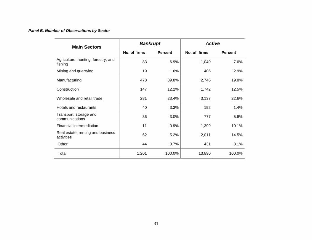
although virtually none is listed in the Colombian stock exchange. Table 1B reports the
sector breakdown. The data cover the period 1996-2003 and contain about 14,000 firms
with close to 70,000 firm-year observations. We refer to this as the sample of active
firms.
We merged our sample of bankrupt firms with the financial data sample using a
firm unique identifier. Out of 1,924 bankrupt firms only 1,201 firms have financial data
in at least one year, resulting in a total of about 5,400 firm-year observations. Our panel
is rather unbalanced and for many firms we only have one or a few years of data
available; some firms have only pre-filing data and some have only post-filing data. The
last three columns of Table 1A give the distribution of these firms with financial data
across three types of proceedings and initial time of the filing.
9

For our bankrupt firms we create a timeline around the time of filing. We refer to
the year of filing as year 0, the first year after filing as +1 and the year before filing as -1.
To study the filing decision, we would like to use financial data at the time of
filing (i.e. year 0). However, for some firms we have no data for the filing year, but have
some data from previous years.10 To increase our sample size we use all firms that have
data for either year 0, -1 or -2. In total, we have 1,032 bankrupt firms with pre-filing
financial data. We refer to this as the bankrupt sample.
In addition to the filing decision, we are interested in comparing the speed of
recovery after filing for reorganization before and after the new law. To do this we
require pre and post filing data for reorganizing firms (since no such data is available for
liquidating firms). To ensure that observed changes in performance are not caused by
changes in sample composition, we construct a sample of firms with available financial
data for the filing year and at least one year pre and post filing. Due to this stricter data
requirement, we have only 322 firms with about 2,000 firm-year observations.11 We refer
to this as our time-series sample.
C. Matched Sample of Active Firms
Our filing data include years with different macroeconomic conditions, including
an episode of major financial crisis in 1999. To control for differences in macroeconomic
conditions affecting our bankrupt firms, we create a matched sample of active firms. For
each firm in our bankrupt sample we pick one active firm that matches the bankrupt firm
by size, year and industry. First, we pick all active firms in the same industry and same
year as the bankrupt firm.12 Then, for each bankrupt firm we find an active firm (among
10 For example, we have 794 firms with data for the filing year. In addition, we have 166 firms with financial data for year -1 (but no data for the filing year) and additional 73 firms have data for year -2 (but no data for year 0 or -1). Note that we do not have data for the year of the filing for any liquidating firms. This is not surprising since once a firm files for liquidation, it does not produce statements for that fiscal year. We have reproduced our main results using only year t-1 for all reorganizing and liquidating firms. The results are similar and thus not reported but available upon request. 11 The time series sample is not statistically different from the larger sample of bankrupt firms on several measures of financial health. However, firms in the time-series sample are larger than firms in the bankrupt sample because larger firms in general have more data available. Thus our results on time-series sample are limited to larger firms. 12 Thus, if a bankrupt firm has data for year 0, we use that year to find a match, but if it has financial data for year -1 or -2, we use that year to find a match.
10
all active firms available in the same year and industry) that is closest in absolute distance
to the size of the bankrupt firm, based on total assets. We make sure that the same active
firm is not assigned to two different bankrupt firms in different years. We end up with
1,032 matched (M) firms (one for each firm in our bankrupt sample), referred to as the
matching sample.
D. Financial Health Variables
We focus on several financial characteristics of the firm. On the liability side, we
calculate the following indebtedness ratios: total liabilities, trade credit, total debt, and
other liabilities13 all scaled by total assets (we refer to these ratios as TL_TA,
TRADE_TA, DEBT_TA, and OTHER LIA_A respectively).
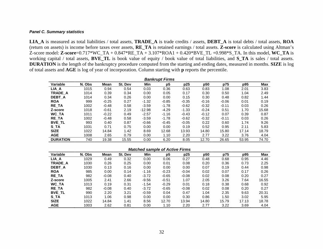
Our main firm characteristic is the Z-score index constructed by Altman (1968)
and updated by Altman (2000). The Z-score is a statistical credit scoring model used to
predict financial distress and the probability of default up to 2 years in advance. The Z-
score combines several indicators of financial fragility, such as the level of indebtedness,
performance and liquidity measures into one composite measure.14
It is important for our purposes that the Z-score is able to separate bankrupt from
healthy firms and serve as a measure of financial health. Our results below show that our
Z-score measure is a strong predictor able to differentiate between active and filing
firms.15
Based on the Altman (2000) model estimated for non-publicly listed firms, the Z-
score is given by:
13 Other liabilities include: government liabilities, worker liabilities, provisions, deferred liabilities and unspecified “other” liabilities category. 14 A concern with this measure is its ability to predict fragility in countries other than the US. Altman argues that “there is no reason why these models (created on US data) cannot be applied to companies throughout the rest of the world” and that he “believes that generic credit risk models are applicable in most environments since the fundamentals of corporate insolvency analysis are relevant everywhere” (Altman 2005). Altman and Hotchkiss (2005) discuss the use of Z-score model in over 20 countries around the world, including many Latin American countries. 15 Although recent research has challenged the use of accounting-based models such as Altman’s in favor of Black-Scholes-Merton default probability models (Hillgeist et al., 2004), these models require stock market data. Unfortunately, most of the firms in our sample are non-listed firms. But even if we had stock market data, it remains to be settled whether the stock market in Colombia is efficient, as BSM default probability models assume. In any event, rather than using the Z-score to predict actual default, we use it a measure of firm financial health in order to assess the impact of the law.
11

Z-score=0.717*WC_TA + 0.847*RE_TA+ 3.107*ROA+ 0.420*BVE_TL+0.998*S_TA
where, WC_TA is working capital (defined as current assets minus current liabilities over
total assets), which is a measure of liquidity, ROA is return on assets (calculated as
income before taxes over total assets), RE_TA is the ratio of retained earnings over
assets, BVE_TL is the ratio of book value of equity over total liabilities (a measure of
indebtedness similar to the ratio of total liabilities to total assets) and S_TA is a ratio of
total sales over total assets. Two performance measures included in the model capture
performance at different horizons – ROA is the performance of the firm in the current
year and RE_TA reflects cumulative performance over time, i.e. firms that continually
have been making losses will have eroded their equity and will report low or negative
retained earnings. We report the results for the composite Z-score, as it presents the
overall measure of financial health and the sub-components of the Z-score. Finally, we
use firm size (calculated as log of total assets) and firm age as controls.
To eliminate influential observations, we clean the data and remove outliers on all
ratios. For ratios that are bounded from below by zero we only remove 1 percent of
outliers on the top. For unbounded ratios we remove 1 percent on the top and the bottom
of the distribution.16 For the Z-score we remove outliers for each individual component
before constructing the Z-score.
Table 1C reports basic summary statistics for our two samples of bankrupt firms
and matched firms. As Table 1C shows, there is no difference in size and age between
bankrupt and matched active firms.
IV. Descriptive Analysis
In this section we present graphical evidence and univariate mean tests. Figure 2
plots kernel density distributions of the Z-score for R (reorganizations), L (liquidations)
16 The exception is the return on assets, for which we remove 2 percent on the top and bottom ends because this variable has very long tails. In addition, for our time-series tests we remove outliers before and after constructing the matched sample.
12
and M (matched active firms) before and after the change in the law. The vertical lines
indicate the mean of each distribution. As Figure 2 shows, before the new law was
introduced, R and L firms have very similar density distributions of Z-scores. Thus, firms
filing for reorganization were not significantly different from the firms filing for
liquidation. However, after the new law was introduced, the differences in the
distributions of R and L firms become more pronounced. Firms that liquidate are now
clearly weaker relative to firms that reorganize. The whole distribution of L-firms shifted
to the left with the new reorganization proceedings. In addition, the sample of matched
active firms seems better off as its kernel density distribution has moved slightly to the
right as compared to before the law. This presents the first evidence in support of
Hypothesis B1.
We further examine the data using univariate mean tests of the variables described
in Section III.D. We first make pair-wise comparisons before and after the law
(comparing R to L firms, R to M firms and L to M firms) and later we make before and
after comparisons for each firm category. Tables 2A and 2B present the results.
Several patterns seem to emerge from the data. Not surprisingly, column 5 of
Table 2A shows that R firms are significantly different from M firms: they have higher
levels of debt (including bank debt and trade credit debt) and lower performance. Their
overall financial health, measured by Z-score, is significantly weaker. In fact, active firms
have on average positive Z-scores, while bankrupt firms have negative Z-scores.
The most interesting result comes from the comparison between R and L before
and after the law. In column 3 of Table 2A we see that R firms are not significantly
different from L firms before the law in 10 out of 11 characteristics reported. The only
difference is in the other liabilities category and, while it’s significant at 5 percent, the
difference is rather small economically (0.16 vs. 0.13). We get a different picture when
we compare R and L after the law: column 8 shows that R firms are significantly
different from L firms in five out of 11 characteristics. Most importantly, R firms differ
from L firms in the composite performance measure – the Z-score. A more thorough look
at sub-components of Z-score reveals that this difference is mainly driven by differences
in RE_TA, significant at 1 percent, and ROA_TA and WC_TA, significant at 10 percent.
After the reform, R firms have better operating performance then L firms, while before
13
the reform there is no difference in operating performance. Furthermore, the differences
are most pronounced in the accumulated performance measure (RE_TA), which shows
that over time L firms have been making more losses than R firms and that these losses
have eroded the equity needed to support their assets. The differences in the level of
indebtedness, measured by the total liabilities to assets or book value of equity over
assets are not significant. There is some difference in trade credit ratios as L firms have
higher trade credit then R firms after the law. As firms get into financial trouble, they are
more likely to extend their trade credit terms and accumulate larger balance on accounts
payables.17 This evidence is in line with our main argument that after the law L firms are
less viable than R firms.
Table 2B presents a different cut of the data – the comparison for each type of
firms before and after the law. The means are the same as in Panel A, but the test for
significance is for before vs. after the reform. We find that L firms have lower Z-score
after the law, which has declined from -0.25 to -0.79, or a difference of -0.54 significant
at 10 percent. This change is driven primarily by one of the five components of the Z-
score - RE_TA – the accumulated losses. However, R firms have better Z-scores after the
law, which has increased from -0.41 to -0.27, a difference of +0.14 also significant at 10
percent. This increase is driven by improvement in ROA and working capital, and slight,
but not significant improvement in BVE, while RE shows a significant decline.
Thus we find that overall, the Z-scores have improved in R firms after the reform
and declined in L firms. In other words, R and L firms move in opposite directions: more
viable firms are more likely to apply for R and less viable firms are more likely to apply
for L after the reform.
Finally, the duration of both liquidations and reorganizations is shorter after the
new law. The difference is much more pronounced for reorganizations, from an average
of 34 months before the law to 12 months after. The difference for liquidations is more
modest, with a change from 49 to 33 months. Recall however that duration can only be
computed if both start and end dates are available. Since liquidations are usually long, our
17 The trade credit patterns for distressed firms are in line with arguments in Fisman and Love (2003) and Love, Prieve and Sarria-Allende (2007). Wilner (2000) argues that suppliers may help customers in financial distress by offering extra trade credit.
14

sample of finished liquidations is biased towards relatively short liquidations, especially
after the law was introduced. We explore these differences more rigorously in Section
V.A.
V. Regression Analysis
A. Duration of Reorganization
In this section we test Hypothesis A1 and A2 discussed in section II.A. We are
interested in comparing the length of reorganization and liquidation cases before and after
the law. The model we use is given by:
Durationi = β1Afteri + β2Ri+ β3Afteri* Ri + Xi’γ + ei, (2)
where After is a dummy equal to one if the filing date occurred after the new law,
R is a dummy for firms filing for reorganization and vector X contains control variables
like firm age and size (because older and larger firms are more complex and may require
longer processing time), industry dummies (to account for differences in technological
process which could be related to differences in complexity of contracts) and Z-score (to
account for the health of the firm at the time of filing, which may also affect the duration
of the process.
Since half of the cases lack ending dates, we assume that these cases are still
unfinished.18 To properly account for these unfinished cases, we estimate a Cox
proportional hazard model. Coefficients in the hazard model of Equation (2) that are
larger than one and significant are to be interpreted as increasing the probability that
cases will end. Therefore, variables associated with positive and significant coefficients
will contribute to shorter durations. The coefficient β1 shows the effect of the new law on
the length of liquidations and therefore tests Hypothesis A2. It should be insignificant.
Coefficient β2 picks up the average difference in the duration between reorganization and
18 The latest closing date in our data is August 3, 2004.
15

liquidations before the law. Finally, β3 picks up the length of reorganization as compared
to liquidations after the law, and if Hypothesis A1 is correct, it should be positive and
significant.
Table 3 reports the hazard ratios from the Cox proportional hazard model in
specification (2). In Column 1 the whole sample of firms for which we have duration data
is used. Column 2 reports the same regression as Column 1 estimated on the sample of
firms with financial data. The rest of columns include additional controls.19
We find that the AFTER coefficient is not significant in any specification. This
implies that there are no differences in the length of liquidations before and after the law
as Hypothesis A2 suggests. Second, reorganization proceedings seem to have shorter
durations, especially after the reform. Before the reform, the marginal probability of
emerging from a reorganization process (at any point in time) is 3 times that of the
probability of ending a liquidation process. However, after the new law, this difference
jumps to 14-25 times (depending on the specification). These results provide strong
evidence that the law reform was very effective in shortening the length of
reorganization, as Hypothesis A1 suggests.
The last specification explores the relationship between duration and Z-score at
the time of filing. We find that while the length of liquidation does not depend on initial
Z-score, healthier firms have shorter reorganizations. This effect is stronger (about twice
as much) after the new law.
B. Selection into Reorganization
To test Hypothesis B1 (described in section II.B) we estimate the following model
after combining the sample of bankrupt firms with the matched sample of active firms:
Yi = β1Afteri + β2Bi+ β3Afteri* Bi + β4Bi*Ri + β5Afteri*Bi*Ri + Xi’γ +ei (3)
19 The number of observations is 1,896. The total number of bankrupt firms is 1,924 as shown in Table 1A. However, 28 observations are dropped either because the start date is missing or the end date comes before the start date.
16
Here Y is one of the six dependent variables described in section III.D, namely,
LIA_A, TRADE_A, DEBT_A, ROA1, RE_TA and Z-score. In addition, B is a dummy
for bankrupt firms (i.e. this dummy is equal to one for either R or L firms) and R is a
dummy for reorganizing firms (a subset of bankrupt firms). We estimate these models by
OLS, with heteroskedasticity-adjusted (White) standard errors.
In this specification, β1 shows the effect of the new law on active companies, β2
shows the difference between bankrupt and active firms, β3 shows the additional
difference between bankrupt and active firms after the new law, β4 shows the difference
between R and L before the new law and β5 shows the same difference after the new law.
The coefficient of interest is β5, the differential impact that the new law had on R versus L
firms.
Table 4 reports our baseline results of the specification given in (3) which
analyzes the financial conditions of firms at the time of filing. We report three main
liability ratios, the five components of the Z-score in Columns 4-8 and the composite Z-
score in Column 9. Bankrupt firms have significantly lower Z-scores relative to active
firms: The t-statistics on the B coefficient in Table 4, model 9 is close to -13. This
suggests that Z-score constructed using US weights has a significant power in predicting
firms in financial distress in Columbia. The difference between bankrupt and active firms
is even more pronounced after the new law as evidenced by the coefficient on After*B
which is negative and significant. At the same time, the After coefficient suggests that
active firms appear in better shape after the new law.
The coefficients of interest are the interactions B*R and After*B*R. The first one
is not significant, suggesting that under the old law there was no significant difference
between financial health of firms filing for reorganization (i.e. R firms) and the firms
filing for liquidation (i.e. L firms). However, the triple interaction is positive and
significant at 5 percent, suggesting that under the new law there is significant difference
between L and R firms and that R firms have higher Z-scores relative to L firms. In other
words, after the new law R firms are significantly healthier relative to L firms.
Next we consider where these differences are coming from. The coefficients show
the relative effect of each additional characteristic – for example, bankrupt firms before
the law relative to matched active firms before the law. To calculate the total effect we
17
need to add the coefficients, as shown in Table 4, Panel B. This table shows the total
difference between each category of filing firms before and after the law, relative to
sample of matched active firms before the law (which is the omitted category in the
regression). We see that R firms have improved by +0.17, while L firms have declined by
-0.68. These numbers closely parallel those reported in Table 2, which showed R firms
improved by 0.14 and L firms declined by -0.54. Thus our multivariate regression results
reaffirm the previous results obtained with simple t-tests.
When we consider the components of the Z-score individually, we find that most
of the effect is coming from RE_TA, mirroring univariate t-tests, which is significant at 5
percent. Two other performance measures, ROA and WC_TA are marginally positive at
about 15 percent and BE_TL is positive with a t-statistics of 1.12 (while not significant at
conventional level, it has the right sign). The liability ratios do not show any relative
difference between R and L firms, while there is a clear difference between filing and
active firms in terms of their level of indebtedness. These results taken together provide
strong evidence for the effectiveness of the new law in separating healthier firms for
reorganization.
We also compare the number of reorganizations that result in mandatory
liquidations before and after the new law. Table 1A shows that about 40 percent of firms
filing for reorganization under the old law ended up in liquidation, while only about 26
percent did so under the new law. This difference is statistically significant with a t-
statistic of close to 6. This result, validating Hypothesis B2, is further evidence that Law
550 contributed to the efficiency of the Colombian bankruptcy system.20,21
20 To be clear, we find that 52 percent (i.e. 25 percent + 75 percent* 36 percent) of firms end up in liquidation before the new law and 43 percent afterwards. In comparison, among small businesses in the US, about 60 percent of Chapter 11 cases end in liquidation or dismissal (which presumably results in liquidation under non-bankruptcy law). See Morrison (2007a). According to Colombian lawyers, these differences are likely to be explained by inefficiency of the liquidation proceedings, before and after the new law, which did not affect the liquidation proceedings. 21 In Djankov et al. (2006), the same hypothetical case of a medium-sized hotel about to default on its debt is presented to bankruptcy lawyers from 88 different countries. Using data on the likely outcome and country level variables, they find that efficiency of debt enforcement is strongly correlated with per capita income and legal origin. Colombia manages to reach the efficient solution despite its French legal origin (which they find to be detrimental to the efficiency) and its relatively low per capita income. Note that at the time the data was collected, the new Law 550 was already in effect. These results square well with our conclusions on improved efficiency of Colombian reorganization process.
18
C. Recovery after Reorganization
Finally, we test whether the new law contributed to a faster recovery of
reorganized firms as described in Hypothesis C, section II.C. Naturally, we do not have
any post filing data for liquidation cases. Presumably these firms closed down or at least
ceased to produce financial statements. Thus, this analysis is done only using
reorganization cases. As already mentioned in Section III.B, the sample for this analysis
is smaller because of limited pre and post-law data availability.
Again, we focus on the Z-score as our main indicator. We expect to obtain
something similar to a V-shape: a declining pattern before the filing as financial health
deteriorates, and an increasing pattern (i.e. recovery) after the filing. We are interested to
see whether this shape is affected by the law reform. Thus, we are interested in the slopes
of time-trend variables. We define two time-trend variables: pre-filing period (Pretrend)
and post-filing period (Posttrend). The Pretrend variable takes values -1, -2, -3 for years
before the filing (and zero otherwise) and the Posttrend variable takes a value of 1 in the
year of filing, a value of 2 in the first year after the filing and so on.
Since the law was passed in 1999, the worst year of the crisis, firms filing after
the law face an expansionary period while those that filed before the law faced the
contraction. Thus, the effect of the overall macroeconomic conditions could be
confounded with the effect of the new law that we are trying to capture. To remedy this
problem, we assume that both bankrupt and active firms are equally affected by the
macroeconomic conditions (we test and confirm this assumption in the next section). Our
dependent variables are therefore defined as the difference in Yit between bankrupt and
matched active firm. The model is given by
DiffYit = β1Afteri + β2Pretrendit+ β3Postrendit+ β4Afteri* Pretrendit + (4)
β5Afteri*Postrendit+Xi’γ +eit.
In this model, β2 shows the slope of DiffYit for years preceding the filing for firms
that filed before the law. Analogously, β3 shows the slope of DiffYit for the years after the
19

filing again for firms that filed before the law. We expect β2 to be negative (i.e. Z-scores
decreasing over time) and β3 to be positive if the firms recover after the reorganization.
The interaction of trends with the After dummy will show differences in pre and post
trend slopes for firms filing after the new law relatively to the slopes on these trends for
firms filing under the old system.
Table 5A reports the average Z-scores for firms filing before and after the law and
Figure 3 plots these means on a graph. We observe a clear pattern of declining Z-scores
before filing, as expected. Financial health deteriorates as firms get closer to the verge of
insolvency. This declining pre-filing pattern is observed for firms filing before and after
the law. However, the recovery patterns are quite different in the two regimes. Before the
law, no clear recovery is observed. Firms that filed for reorganization, if anything, are
getting worse. In contrast, the recovery is very pronounced after the introduction of Law
550, with a clear upward trend in the years following the filing.
Table 5B presents the regression analysis corresponding to the graphical evidence
just described. The Pretrend coefficient shows how steeply financial conditions worsen
before the filing (relative to matched firms). We expect a negative coefficient on the Z-
score and its components, as lower values indicate worse financial health. However, we
expect a positive coefficient on liability ratios since higher ratios indicate worse financial
health. As expected, the Pretrend coefficient is negative for four out of the five Z-score
components (ROA, RE_TA, WC_TA and S_TA) and is positive for the leverage
measures, suggesting that before the filing, leverage is increasing while performance is
deteriorating.
There is some difference in pre-trend patterns before and after the law shown by
the interaction of Pretrend and After (coefficient β4). Specifically, declines in
performance after the new law, measured as ROA, RE_TA, WC_TA or S_TA are not as
steep as declines before the law – the interaction of Pretrend and After are positive for
these measures and significant at 5 percent (except RE_TA which is only significant at 15
percent). In other words, judging by performance measures, firms filing after the new law
appear healthier compared to those that filed before the law. Note that this is relative to
the sample of matched active firms in the same years, which controls for aggregate
economic conditions.
20
The Postrend coefficient shows how fast the firms recover after the filing relative
to the performance of the matched firm over the same time period. There is no clear
pattern of improvement under the old law. The overall Z-score measure shows no
improvement, while individual measures point in different directions –improvement in
ROA and S_TA, but declines in RE_TA and BE_TA. The Liability ratios also reveal a
mixed picture, with a significant decline in debt levels (which is plausible if banks were
reluctant to lend or roll-over the loans after the filing), but with increases in the levels of
trade credit, as firms try to substitute bank credit for informal finance from their
suppliers. The overall impact is an increase in liabilities ratios and reduction in equity
values.
The main variable of interest is the relative difference in post-filing performance
before and after the law, which is captured by the interaction of Postrend and After
(coefficient β5). This coefficient is significantly positive for the Z-score, which shows
that after the law firms recover faster than before the new law (i.e. the slope is steeper).
However, this effect is mainly driven by one component of the Z-score: BVE_TL, book
value of equity over total liabilities. Thus, the differences in recovery patterns before and
after the new law are mainly driven by increase in equity value, relative to liabilities.
Therefore, we argue that after the new law, the reorganization process results in a
more pronounced recovery in the years following the filing. This is in stark contrast to the
post-filing pattern under the old law, which showed a continuous deterioration in firm
performance. Note that the impact of macroeconomic conditions is captured by matching
active firms because our dependent variables are defined as differences with active firms.
This evidence validates our Hypothesis C. 22
To be clear, the reform has impacted firms in the intensive margin, that is, firms
that would have filed for bankruptcy irrespective of the law, as well as firms in the
extensive margin, that is, firms that would have resolved disputes outside the bankruptcy
proceedings (which is commonly known as “workouts”) but are now filing for
22 Because our time-series sample includes larger firms (that have pre and post filing data), the results presented here are only applicable to larger firms. While this is an important finding, more research is needed to discern if the reform improved post-filing performance for smaller firms.
21
bankruptcy thanks to the reform.23 Therefore our results show the combined effect of the
reform on both types of firms. We do not have the data on outside workouts to determine
which of these effects dominate.
VII. Robustness to Crisis and Trend
As mentioned earlier, the new law was introduced in the midst of a major
financial crisis in late 1999. For our identification strategy to work, we need to make sure
that the crisis did not have a differential effect on R relative to L firms. In addition, the
crisis might make it more difficult to distinguish viable firms from unviable ones. We
need to make sure that the effects we observe after the introduction of the law are not due
to the crisis.
We control for the crisis by creating two windows: year 1999 (the worst year of
the crisis) and years 1998-2000, which span the worst crisis year. Fortunately, since our
sample covers 1996-2003, we have several years outside of the crisis window on both
sides (before and after the law), which allows us to test whether our results are influenced
by the crisis. Figure 1 shows that crisis was largely limited to 1999, which was the only
year with negative GDP growth.
Another potential concern with our results is that the effect that we attribute to the
law reform could actually come from a gradual improvement in the efficiency of the
bankruptcy system over time and not to a one-time event such as the adoption of the new
law. To test for this possibility, we create a linear time trend and use it in interactions in
the same fashion as our After variable.
The crisis and trend regressions are presented in Table 6A for our duration results
and Table 6B for Z-score. We present several specifications to test the robustness of our
23 Workouts is a common practice in the US, see Gertner and Scharfstein (1991), Mann (2005) and Morrison (2007b). Workouts also exist in Colombia although they are rarely used according to private communication with Colombian lawyers and Rouillon (2006). Part of the reason may be that the old law provided a “safe haven” for debtors, who preferred filing for bankruptcy to negotiating voluntarily with their creditors.. The fact that more firms apply for reorganization after the law also suggest that the incentives of the new law were more aligned toward using the formal process rather than out of court restructuring.
22
results. In both tables, the first column reproduces the baseline specification for
comparison: in Table 6A it is model 1 from Table 3 and in Table 6B it is model 9 from
Table 4. Model 2 adds the trend, Model 3 adds Crisis99 and its interactions, Model 4
adds Crisis98_00. In models 5 and 6 we test crisis and trend together using both crisis
windows. In models 7 and 8 we return to our baseline specification but drop the relevant
crisis years from the regression.
In the first sets of results on duration, we find that our main interactions with
After*R (Table 6A) and After*B and After*B*R (in Table 6B) remain significant in all
the specifications, suggesting that the difference between the pre-reform and post-reform
periods is not related to the financial crisis.
In Table 6B we see that the Crisis99 dummy is significant and negative,
suggesting that all firms – active, liquidating and reorganizing, fared worse during 1999.
The Crisis98_00 dummy is not significant (model 4), so the crisis seems limited to 1999.
More importantly, the interactions of the crisis dummies with the type of firms, namely
Crisis*B and Crisis*B*R are both insignificant, suggesting that crisis did not have any
differential effect on bankrupt firms (relative to active) or R firms relative to L firms.
Since Crisis has the same effect on the whole distribution of firms, our identification
strategy, which compares bankrupt to active and R to L, is valid.
Finally, we address another source of bias – the possibility that it is more difficult
to distinguish viable from nonviable firms during recessions than during recovery
periods. If this were the case, then filings that occurred during recession years would be
different from filings that occurred in normal years. We rerun our baseline model
dropping year 1999 (in model 7) and, to be conservative, we also drop the year before
and after the recession year. That is, we drop 1998-2000 (in model 8). We find that our
results are not driven by the abnormalities related to the recession period. Even though
the number of observations drops significantly, we still observe a positive relative
difference between R and L firms in normal years after the reform but not before the
reform.
It is important to reiterate that the results presented in Section VI.C on recovery
after reorganization are not confounded by the crisis because the dependent variables are
defined as the difference between the bankrupt firms and the matched sample of active
23
firms. From the results reported above we know that the crisis did not have any
differential effects on Z-scores of bankrupt relative to active firms. Thus, the difference
in recovery is a result of the law because the crisis effect is differenced out.
VII. Conclusions
This paper studies the role that the length of reorganization plays in the efficiency
of bankruptcy laws. We hypothesized that in a regime with high costs (or lengthy
reorganizations), the law fails to achieve the efficient outcome of liquidating unviable
business and reorganizing viable ones. However, when bankruptcy costs are low,
bankruptcy laws can serve its filtering purpose. We test the hypothesis using Colombia as
an example. In 1999, amidst a major crisis, the Colombian Congress replaced the existing
corporate reorganization proceeding with a more streamlined procedure that limited
negotiations to a maximum of eight months and stipulated that failure to reach an
agreement would result in mandatory liquidation.
We use data from all filing firms in Colombia between 1996 and 2003, spanning
the change in the reorganization law, to provide evidence that the new law increased the
efficiency of the bankruptcy system in Colombia. We first confirm that indirect
reorganization costs, as measured by the duration of the reorganization process, have
significantly decreased after the reform as intended. Second, we show that the pre-reform
reorganization proceedings were so inefficient that they failed to separate economically
viable firms from inefficient ones. In contrast, by imposing a statutory deadline on the
length of reorganizations, the new law succeeds in selecting healthier (and hence more
viable) firms filing for reorganization. Finally, we show that the recovery of reorganized
firms is significantly improved after the reform, as a result of the statutory deadline and
the better selection of viable firms that ensued.
Although we only analyze a change in the indirect costs of reorganization, we
believe that from a policy standpoint, this paper highlights the relevance of the design of
bankruptcy laws. A reduction in the costs (both direct and indirect) associated with filing
can contribute to the overall efficiency of the economy and should be a priority in the
agenda for economic reforms.
24
Appendix 1. Background on Colombian Bankruptcy Law Reform.24
In 1995, the Law 222 was enacted in an attempt to reduce the judiciary burden by
allowing disputes among creditors and debtors to be resolved under the Superintendence
of Companies. In addition, the superintendence, under the Ministry of Industry and
Commerce, is in charge of supervising firms to prevent insolvency and fraud. The law
established the procedures for both mandatory liquidation and restructuring under the
Concordato proceedings. Voluntary liquidation was and is still regulated by the
Commercial Code.
Before Law 222, mandatory liquidations were civil bankruptcy proceedings that
lasted for many years because civil courts lacked capacity and specific business
knowledge. Under Law 222, however, mandatory liquidation proceedings are still
lengthy, usually taking more than three years to resolve. The length of the proceedings in
practice implies that a substantial part of the assets of the debtor are lost either because
they lose value over time (indirect cost) or are spent towards paying the fees and
expenses of the liquidation (direct costs). As a result, the perception is that mandatory
liquidation is very inefficient.
Although more authority was given to the superintendence, the Concordato
proceedings under Law 222 still suffered from being excessively long. In essence, too
much leverage was given to the debtor in the negotiations with creditors. Delays were
favorable to debtors as they allowed them to suspend the debt service, and also granted
protection by the stay against execution actions commenced by creditors (Tamayo et al.,
2002).
Some creditors tried to strike private agreements with the managers, outside the
scope of the Concordato. These agreements were typically used to restructure and
reschedule the debtor’s obligations but are considered onerous by both parties as it is
difficult to reach agreements. In Colombia, they are regulated by the general Civil Law
under the principle of freedom of will of all the parties involved.
Starting in 1998 after decades of consistent growth, the Colombian economy
24 This Section draws from Urrutia (2004).
25

suffered a major recession. The severity of the crisis forced the government to propose
several bills to Congress. One of them replaced the sections of Law 222 that concerned
the reorganization proceeding and became known as Law 550 after it was approved by
Congress in December of 1999.
The Law 550 applies to all types of companies, regardless of their organizational
nature, except for financial institutions. The entity responsible for conducting the
proceedings is the Superintendence of Companies25 as was the case under Law 222, or
the relevant superintendence in charge of its supervision.
The Acuerdo, or reorganization proceeding under Law 550, is divided into two
major phases during which the management of the bankrupt firm remains in charge. The
first consists of the determination of votes and claims according to the parties’ stake in
the firm. In the second, the negotiation and voting of the reorganization plan takes place.
Each phase may last for a maximum of 4 months and failure to meet the deadline results
in mandatory liquidation.
After a reorganization case was filed under old Law 222, the superintendence
appointed a controller and a provisional committee of creditors. Past experience showed
that the creditors committee and the controller interfered many times with the task of
managing the company. Therefore, Law 550 eliminates the need to appoint a creditors
committee and the controller for the proceedings. Instead, the Law 550 creates the figure
of the promoter, an independent person also appointed by the relevant superintendence.26
The promoter gathers and analyzes business and financial information of the debtor,
compiles a complete list of creditors, facilitates the negotiations among the creditors,
conceives the restructuring plan and coordinates the voting process for approval of the
restructuring agreement. The promoter participates actively in the negotiations and
determines the voting rights among the parties involved. For his or her services, the
promoter is paid a success fee, thus having a stake in ensuring that an agreement will be
reached.
25 Although the proceedings are administrative rather than judicial, Law 550 grants to the superintendence the power and authority to make certain decisions which have the force of a final judgment. 26 Sometimes, creditors and debtor may suggest a candidate for consideration, and practice has shown that when this happens, the Superintendent accepts the candidate suggested.
26
Under Law 222, any Concordato agreement had to be approved by the debtor. In
practice, this implied that the debtor effectively had the veto power, regardless of his or
her stake in the firm. To solve this problem, Law 550 establishes that shareholders of the
debtor company are “internal creditors”, one of the five different classes27 of creditors
among which voting rights are distributed according to their claims to the firm.
The number of votes needed to approve a reorganization plan also changed.
Under Law 222, the Concordato required a majority vote of 75 percent of all creditors
recognized in the proceedings, which many times became an insurmountable obstacle due
to lack of interest of certain creditors which simply neglected to participate in the
proceedings. In contrast, under Law 550 the Acuerdo only requires a 51 percent majority
of the eligible votes of creditors to approve the restructuring agreement.
Although Law 550 is an important improvement with respect to the previous law,
a report commissioned by the superintendence shows some dissatisfaction among firms
that filed for reorganization with regards to access to fresh credit. It thus seems that banks
are still reluctant to give credit to firms under reorganization.
In addition, several practitioners in Colombia have pointed out some
improvements that if introduced could result in lower coordination costs among creditors
and debtors and therefore lead to faster agreements. Currently under Law 550, once the
reorganization plan is approved with the required majority of creditors, it is binding by all
parties. Dissenting creditors may file lawsuits before the relevant superintendence but this
is problematic as small creditors may object to the plan delaying its implementation
although their claim is relatively small.
Law 550 was to be in force only for a five year term. The government and
Congress approved a bill that extended the application of Law 550 until December 2006,
while Congress discussed the new insolvency draft law, which came into effect as Law
1116 on June 28th, 2007.
27 Claims are classified by the law both for purposes of voting and priority of claims. There are five different classes of creditors: Internal creditors, External creditors, Employees and retired employees, Governmental entities, Financial institutions. For purposes of priority the classification is that of the Civil Code.
27

REFERENCES
Adler, Barry E. 1997. A Theory of Corporate Insolvency. New York University Law Review 72, 343-382.
Aghion, P., O. Hart and J. Moore, 1992, The economics of bankruptcy reform, Journal of Law and Economics 8, 523-546.
Alderson, M.J. and B.L. Betker, 1995, Liquidation costs and capital structure, Journal of Financial Economics 39, p. 45-69.
Altman, E.I., 1968, Finanical ratios, discriminant analysis and the prediction of corporate bankruptcy, Journal of Finance 23, 589-609.
______, 1984, A further empirical investigation of the bankruptcy cost question, Journal of Finance 39, 1067-1089.
______, 2000, Predicting financial distress of companies: Revisiting the Z-score and Zeta Models, Stern School of Business, New York University, mimeo.
______, 2005, An emerging market credit scoring system for corporate bonds, Emerging Markets Review vol, 6(4), 311-323.
______, Hotchkiss, E., 2005. Corporate Financial Distress and Bankruptcy. 3rd edition. John Wiley & Sons, New York.
Baird, D. G, 1986, The uneasy case for corporate reorganizations, Journal of Legal Studies 15, 125-147.
Baird, D. G. and R. Picker, 1991, A Simple Noncooperative Bargaining Model of Corporate Reorganizations. Journal of Legal Studies 20, 311-349.
Bris, A., I. Welch and N. Zhu, 2006, The Costs of Bankruptcy: Chapter 7 Liquidation vs. Chapter 11 Reorganization, Journal of Finance 61, 1253-1303.
Claessens, S., Djankov, S., Mody, A., and Stiglitz, J. 2001, Resolution of Financial Distress: An international Perspective on the Design of Bankruptcy Laws, An overview and Chapter 1.
______, and Klapper, L. F., 2003, Bankruptcy around the world: explanations of its relative use, The World Bank, Policy Research Working Paper Series, 1-42.
Davydenko, S and J. Franks, 2005, Do Bankruptcy Codes Matter? A Study of Defaults in France, Germany and the UK, Finance Working paper 89/2005, European Corporate Governance Institute.
Djankov, S., O. Hart, C. McLiesh, and A. Shleifer, 2006, Debt Enforcement Around the World, mimeo, World Bank.
Fisman, R., and Love, I., 2003, Trade Credit, Financial Intermediary Development and Industry Growth, Journal of Finance 58, 353-374.
Franks J.R. and G. Loranth, 2005, “A Study of Inefficient Going Concerns in Bankruptcy.” CEPR Discussion Paper 5035, Centre for Economic Policy Research, London.
______ and Torous, W.N., 1989, An empirical investigation of U.S. firms in reorganization, Journal of Finance 44, 747-769.
Hart, O., 2000 Different Approaches to Bankruptcy, NBER working paper 7921. Hillegeist, S.A, Keating, E.K., Cram, D.P., and Lundstedt, K.G., 2004, Assessing the
probability of bankruptcy, Review of Accounting Studies 9, 5-34. Hotchkiss, Edith S., 1995, Post-bankruptcy performance and management turnover,
Journal of Finance 50, 3-21. Gertner, R. and D. Scharfstein, 1991, A theory of workouts and the effects of
reorganization law, Journal of Finance 4, 1189-1221. Giné, X. and I. Love, 2006, “Do Reorganization Costs Matter for Efficiency?
Evidence from a Bankruptcy Reform in Colombia” Working Paper Series 3970, World Bank, Washington, DC.
28

29
Love, Inessa, Lorenzo A. Preve and Virginia Sarria-Allende, 2007, “Trade Credit and Bank Credit: Evidence from Recent Financial Crises, Journal of Financial Economics, vol. 83, issue 2, February 2007, pp. 453-469.
Maksimovic, V. and M.G. Phillips, 1998, Asset efficiency and reallocation decisions of bankrupt firms, Journal of Finance 53, 1495-1532.
Mann, Ronald J. 2004. An Empirical Investigation of Liquidation Choices of Failed High-Tech Firms. Washington University Law Quarterly 82: 1375.
Morrison, E.R. 2007a, Bankruptcy Decision Making: An Empirical Study of Continuation Bias in Small-Business Bankruptcies. Journal of Law & Economics 50, 381-419.
Morrison, Edward R. 2007b, Bargaining Around Bankruptcy: Small Business Workouts and State Law. Working paper. Columbia Law School.
Rouillon, A, 2006, “Colombia: Creditor Rightrs and insolvency Proceedings”, World Bank, Washington, DC.
Shleifer, A., and Vishny, R.W., 1992, Liquidation values, and debt capacity: A market equilibrium approach, Journal of Finance 47, 1343-1366.
Smith, D.C., and Strömberg, P., 2004, Maximizing the value of distressed assets: Bankruptcy law and the efficient reorganization of firms, prepared for the World Bank conference on Systematic Financial Distress.
Stromberg, P., 2000, Conflicts of Interest and Market Illiquidity in Bankruptcy Auctions: Theory and Tests, Journal of Finance 55, 2641-2692.
Schwartz, Alan. 1997. Contracting About Bankruptcy. Journal of Law, Economics & Organization 13, 127-146.
Tamayo, D. F. Visbal and M. Nuñez, 2002, El Sesgo Anti-Acreedor en los Contratos de Garantía y en los Procesos de Reestructuración de la Ley 550 de 1999. In González Muñoz, C., A. García and A. Carrasquillo, El Sector Financiero de Cara al Siglo XXI, ANIF, Bogotá.
Thorburn, K.S., 2000, Bankruptcy auctions: Costs, debt recovery and firm survival, Journal of Financial Economics 58, 337-368.
Uribe, J.D. and H. Vargas, 2002, Financial Reform, Crisis and Consolidation in Colobmia, Borradores de Economía 204, Banco de la República, Colombia.
Urrutia, C, 2004 Insolvency Reform in Colombia, prepared for the World Bank, Brigard & Urrutia, Bogotá, Colombia.
Urrutia, M and Zárate, J.P 2001, La Crisis Financiera de Fin de Siglo, Banco de la República, Colombia.
White, M.J., 1989, The corporate bankruptcy decision, Journal of Economic Perspectives 3, 129-151.
Weiss, Lawrence, A., 1990, Bankruptcy resolution: Direct costs and violation of priority of claims, Journal of Financial Economics 27, 285-314.
______, and K.H. Wruck, 1998, Information problems, conflicts of interest and asset stripping: Chapter 11’s failure in the case of Eastern Airlines, Journal of Financial Economics 48, 55-97.
Wilner, B., 2000. The exploitation of relationships in financial distress: the case of trade credit. Journal of Finance 55, 153-178.
World Bank, 2006, Closing a business, Doing business in 2006: Creating Jobs, 67-76. ______, 2005, Closing a business, Doing business in 2005: Removing Obstacles to
Growth, 67-78. ______, 2004, Closing a business, Doing business in 2004: Understanding
Regulations, 71-103, 112-114.

Table 1. Data availability The first four columns report the number of firms with existing bankruptcy data. The last three columns report the number of firms with existing bankruptcy and financial data and in parenthesis the total number of years of data for these firms. The first and fifth column report the total number of observations, the third and sixth the number of firms that filed before 2000, under the old law, and the fourth and seventh the number of firms that filed after 2000 under the new law. The second column reports the number of reorganizations that ended in mandatory liquidation.
Panel A. Number of Observations by Bankruptcy Case
Bankruptcy Data Number of firms
Financial Data Number of firms
(Number of firm - year obs.)
Cases Description Total Mandatory Liquidation Before After Total Before After
ACUERDOS Reorganization under Law 550 780 184 0 780 561 (2,651)
0 (0)
561 (2,651)
CONCORDATOS Reorganization under Law 222 590 214 590 0 441 (2,152)
441 (2,152)
0 (0)
LIQUIDACIONES Liquidation under Law 222 554 - 283 271 199 (547)
88 (158)
111 (389)
TOTAL BANKRUPT FIRMS Firms that filed for bankruptcy
1,924
398
873 1,051 1,201
(5,350) 529
(2,310) 672
(3,040)
TOTAL ACTIVE FIRMS
Firms that never filed bankruptcy 13,891
(68,298)
(35,054)
(33,244)
30
Panel B. Number of Observations by Sector
Bankrupt Active Main Sectors
No. of firms Percent No. of firms Percent
Agriculture, hunting, forestry, and fishing 83 6.9% 1,049 7.6%
Mining and quarrying 19 1.6% 406 2.9%
Manufacturing 478 39.8% 2,746 19.8%
Construction 147 12.2% 1,742 12.5%
Wholesale and retail trade 281 23.4% 3,137 22.6%
Hotels and restaurants 40 3.3% 192 1.4%
Transport, storage and communications 36 3.0% 777 5.6%
Financial intermediation 11 0.9% 1,399 10.1%
Real estate, renting and business activities 62 5.2% 2,011 14.5%
Other 44 3.7% 431 3.1%
Total 1,201 100.0% 13,890 100.0%
31
Panel C. Summary statistics LIA_A is measured as total liabilities / total assets, TRADE_A is trade credits / assets, DEBT_A is total debts / total assets, ROA (return on assets) is income before taxes over assets, RE_TA is retained earnings / total assets. Z-score is calculated using Altman’s Z-score model: Z-score=0.717*WC_TA + 0.847*RE_TA + 3.107*ROA1 + 0.420*BVE_TL +0.998*S_TA. In this model, WC_TA is working capital / total assets, BVE_TL is book value of equity / book value of total liabilities, and S_TA is sales / total assets. DURATION is the length of the bankruptcy procedure computed from the starting and ending dates, measured in months. SIZE is log of total assets and AGE is log of year of incorporation. Column starting with p reports the percentile.
Bankrupt Firms Variable N. Obs Mean St. Dev Min p5 p25 p50 p75 p95 Max LIA_A 1015 0.94 0.54 0.03 0.36 0.63 0.83 1.08 2.01 3.83 TRADE_A 1014 0.39 0.34 0.00 0.05 0.17 0.30 0.50 1.04 2.49 DEBT_A 1014 0.34 0.26 0.00 0.00 0.15 0.30 0.48 0.82 1.44 ROA 999 -0.25 0.27 -1.32 -0.85 -0.35 -0.16 -0.06 0.01 0.19 RE_TA 1002 -0.48 0.58 -3.59 -1.78 -0.62 -0.32 -0.11 0.03 0.26 Z-score 1018 -0.61 2.19 -12.98 -4.29 -1.33 -0.24 0.51 1.70 15.68 WC_TA 1011 -0.22 0.49 -2.57 -1.16 -0.43 -0.12 0.07 0.39 0.87 RE_TA 1002 -0.48 0.58 -3.59 -1.78 -0.62 -0.32 -0.11 0.03 0.26 BVE_TL 993 0.40 0.87 -0.66 -0.45 -0.05 0.22 0.60 1.74 9.26 S_TA 1031 0.71 0.75 0.00 0.00 0.19 0.52 0.95 2.11 5.83 SIZE 1022 14.84 1.42 8.69 12.68 13.93 14.80 15.80 17.14 18.79 AGE 1008 2.65 0.79 0.00 1.10 2.20 2.77 3.22 3.76 4.04 DURATION 740 19.38 15.55 0.00 6.20 8.05 12.70 26.65 53.95 74.70
Matched sample of Active Firms Variable N. Obs Mean St. Dev Min p5 p25 p50 p75 p95 Max LIA_A 1029 0.49 0.32 0.00 0.06 0.27 0.48 0.68 0.95 4.46 TRADE_A 1030 0.26 0.25 0.00 0.01 0.08 0.20 0.36 0.73 2.25 DEBT_A 1030 0.13 0.16 0.00 0.00 0.00 0.07 0.19 0.44 0.98 ROA 985 0.00 0.14 -1.16 -0.23 -0.04 0.02 0.07 0.17 0.26 RE_TA 982 -0.08 0.40 -3.72 -0.65 -0.08 0.02 0.08 0.20 0.27 Z-score 1005 2.41 2.66 -9.56 -0.51 1.07 2.05 3.26 7.64 16.55 WC_TA 1013 0.19 0.31 -1.54 -0.29 0.01 0.18 0.38 0.68 0.92 RE_TA 982 -0.08 0.40 -3.72 -0.65 -0.08 0.02 0.08 0.20 0.27 BVE_TL 990 2.20 3.21 -0.59 0.04 0.47 1.04 2.35 9.63 20.31 S_TA 1013 1.06 0.98 0.00 0.00 0.30 0.86 1.50 3.02 5.95 SIZE 1022 14.84 1.41 8.56 12.70 13.94 14.80 15.79 17.13 18.78 AGE 1003 2.62 0.81 0.00 1.10 2.20 2.77 3.22 3.69 4.04
32

Table 2. Mean tests R firms are those that filed for reorganization, L firms filed for liquidation, and M is the matched sample of active firms. We mark the difference with ***, ** or * to indicate significance at the 1, 5 or 10 percent level, respectively. See Table 1 for definition of variables. Panel A. Pair wise comparison of R, L, and M firms before and after the law Before the Law After the Law L R R vs. L M R vs. M L R R vs. L M R vs. M Variable (1) (2) (3) (4) (5) (6) (7) (8) (9) (10) LIA_A 0.85 0.86 NS 0.52 *** 0.92 0.85 NS 0.49 ***
TRADE_A 0.31 0.35 NS 0.28 *** 0.48 0.39 * 0.27 *** DEBT_A 0.38 0.38 NS 0.15 *** 0.29 0.3 NS 0.13 *** OTHER LIA_A 0.16 0.13 ** 0.09 *** 0.16 0.16 NS 0.09 ***
SIZE 14.89 14.84 NS 14.88 NS 14.87 15.19 NS 15.15 NS Z-score components:
ROA1 -0.23 -0.25 NS -0.01 *** -0.27 -0.2 * 0.01 *** RE_TA -0.33 -0.37 NS -0.04 *** -0.73 -0.44 *** -0.08 *** WC_TA -0.16 -0.21 NS 0.19 *** -0.26 -0.14 * 0.16 *** BVE_TL 0.46 0.41 NS 1.84 *** 0.27 0.44 NS 2.34 *** S_TA 0.67 0.67 NS 1.05 *** 0.73 0.65 NS 1.13 ***
Z-score -0.25 -0.41 NS 1.89 *** -0.79 -0.27 ** 2.17 *** N Obs. 109 363 451 29 422 429 Duration 48.62 34.1 *** 33.2 11.7 ***
33

Panel B. Before and after the law comparison by firm category R L M Before After Sign. Before After Sign. Before After Sign. Variable (1) (2) (3) (4) (5) (6) (7) (8) (9) LIA_A 0.86 0.85 NS 0.85 0.92 NS 0.52 0.49 **
TRADE_A 0.35 0.39 ** 0.31 0.48 *** 0.28 0.27 NS DEBT_A 0.38 0.3 *** 0.38 0.29 ** 0.15 0.13 *** OTHER LIA _ A 0.13 0.16 *** 0.16 0.16 NS 0.09 0.09 NS
SIZE 14.84 15.19 *** 14.89 14.87 NS 14.88 15.15 *** Z-score components:
ROA1 -0.25 -0.2 *** -0.23 -0.27 NS -0.01 0.01 ** RE_TA -0.37 -0.44 ** -0.33 -0.73 *** -0.04 -0.08 ** WC_TA -0.21 -0.14 ** -0.16 -0.26 NS 0.19 0.16 ** BVE_TL 0.41 0.44 NS 0.46 0.27 NS 1.84 2.34 *** S_TA 0.67 0.65 NS 0.67 0.73 NS 1.05 1.13 NS
Z-score -0.41 -0.27 * -0.25 -0.79 * 1.89 2.17 *** N Obs. 363 422 109 29 451 429 Duration 34.1 11.7 *** 48.6 33.2 ***
34
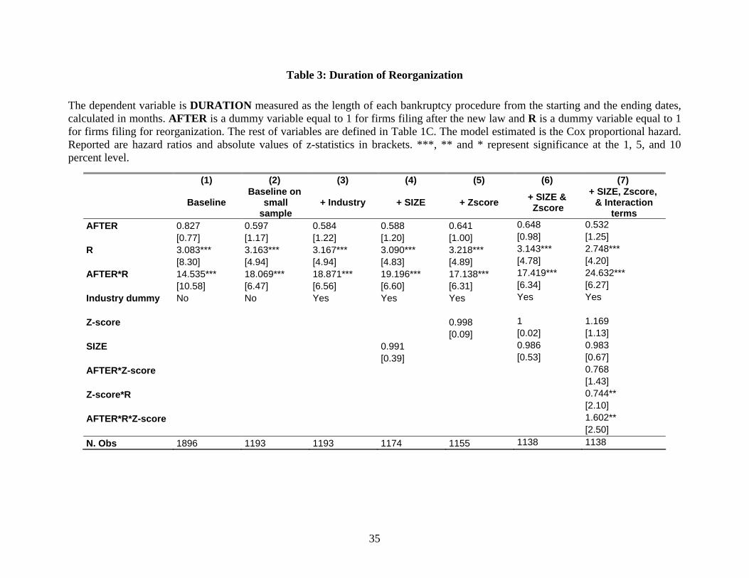
Table 3: Duration of Reorganization
The dependent variable is DURATION measured as the length of each bankruptcy procedure from the starting and the ending dates, calculated in months. AFTER is a dummy variable equal to 1 for firms filing after the new law and R is a dummy variable equal to 1 for firms filing for reorganization. The rest of variables are defined in Table 1C. The model estimated is the Cox proportional hazard. Reported are hazard ratios and absolute values of z-statistics in brackets. ***, ** and * represent significance at the 1, 5, and 10 percent level.
(1) (2) (3) (4) (5) (6) (7)
Baseline Baseline on
small sample
+ Industry + SIZE + Zscore + SIZE & Zscore
+ SIZE, Zscore, & Interaction
terms AFTER 0.827 0.597 0.584 0.588 0.641 0.648 0.532 [0.77] [1.17] [1.22] [1.20] [1.00] [0.98] [1.25] R 3.083*** 3.163*** 3.167*** 3.090*** 3.218*** 3.143*** 2.748*** [8.30] [4.94] [4.94] [4.83] [4.89] [4.78] [4.20] AFTER*R 14.535*** 18.069*** 18.871*** 19.196*** 17.138*** 17.419*** 24.632*** [10.58] [6.47] [6.56] [6.60] [6.31] [6.34] [6.27] Industry dummy No No Yes Yes Yes Yes Yes Z-score 0.998 1 1.169 [0.09]
[0.39]
[0.02] [1.13] SIZE 0.991 0.986 0.983 [0.53] [0.67] AFTER*Z-score 0.768 [1.43] Z-score*R 0.744** [2.10] AFTER*R*Z-score 1.602** [2.50] N. Obs 1896 1193 1193 1174 1155 1138 1138
35
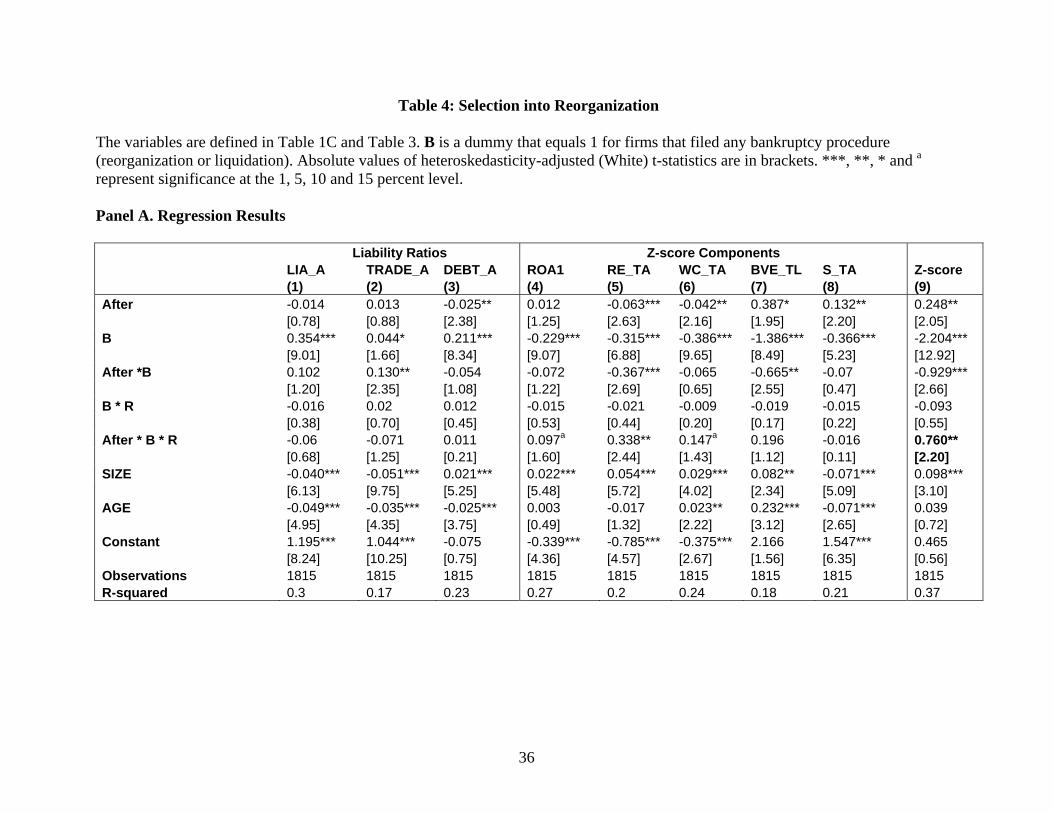
Table 4: Selection into Reorganization The variables are defined in Table 1C and Table 3. B is a dummy that equals 1 for firms that filed any bankruptcy procedure (reorganization or liquidation). Absolute values of heteroskedasticity-adjusted (White) t-statistics are in brackets. ***, **, * and a represent significance at the 1, 5, 10 and 15 percent level. Panel A. Regression Results Liability Ratios Z-score Components LIA_A TRADE_A DEBT_A ROA1 RE_TA WC_TA BVE_TL S_TA Z-score (1) (2) (3) (4) (5) (6) (7) (8) (9) After -0.014 0.013 -0.025** 0.012 -0.063*** -0.042** 0.387* 0.132** 0.248** [0.78] [0.88] [2.38] [1.25] [2.63] [2.16] [1.95] [2.20] [2.05] B 0.354*** 0.044* 0.211*** -0.229*** -0.315*** -0.386*** -1.386*** -0.366*** -2.204*** [9.01] [1.66] [8.34] [9.07] [6.88] [9.65] [8.49] [5.23] [12.92] After *B 0.102 0.130** -0.054 -0.072 -0.367*** -0.065 -0.665** -0.07 -0.929*** [1.20] [2.35] [1.08] [1.22] [2.69] [0.65] [2.55] [0.47] [2.66] B * R -0.016 0.02 0.012 -0.015 -0.021 -0.009 -0.019 -0.015 -0.093 [0.38] [0.70] [0.45] [0.53] [0.44] [0.20] [0.17] [0.22] [0.55] After * B * R -0.06 -0.071 0.011 0.097a 0.338** 0.147a 0.196 -0.016 0.760** [0.68] [1.25] [0.21] [1.60] [2.44] [1.43] [1.12] [0.11] [2.20] SIZE -0.040*** -0.051*** 0.021*** 0.022*** 0.054*** 0.029*** 0.082** -0.071*** 0.098*** [6.13] [9.75] [5.25] [5.48] [5.72] [4.02] [2.34] [5.09] [3.10] AGE -0.049*** -0.035*** -0.025*** 0.003 -0.017 0.023** 0.232*** -0.071*** 0.039 [4.95] [4.35] [3.75] [0.49] [1.32] [2.22] [3.12] [2.65] [0.72] Constant 1.195*** 1.044*** -0.075 -0.339*** -0.785*** -0.375*** 2.166 1.547*** 0.465 [8.24] [10.25] [0.75] [4.36] [4.57] [2.67] [1.56] [6.35] [0.56] Observations 1815 1815 1815 1815 1815 1815 1815 1815 1815 R-squared 0.3 0.17 0.23 0.27 0.2 0.24 0.18 0.21 0.37
36
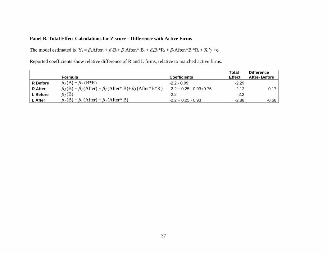
Panel B. Total Effect Calculations for Z score – Difference with Active Firms
The model estimated is Yi = β1Afteri + β2Bi+ β3Afteri* Bi + β4Bi*Ri + β5Afteri*Bi*Ri + Xi’γ +ei Reported coefficients show relative difference of R and L firms, relative to matched active firms.
Formula Coefficients Total Effect
Difference After- Before
R Before β2 (B) + β4 (B*R) -2.2 - 0.09 -2.29 R After β2 (B) + β1 (After) + β3 (After* B)+ β5 (After*B*R ) -2.2 + 0.25 - 0.93+0.76 -2.12 0.17L Before β2 (B) -2.2 -2.2 L After β2 (B) + β1 (After) + β3 (After* B) -2.2 + 0.25 - 0.93 -2.88 -0.68
37
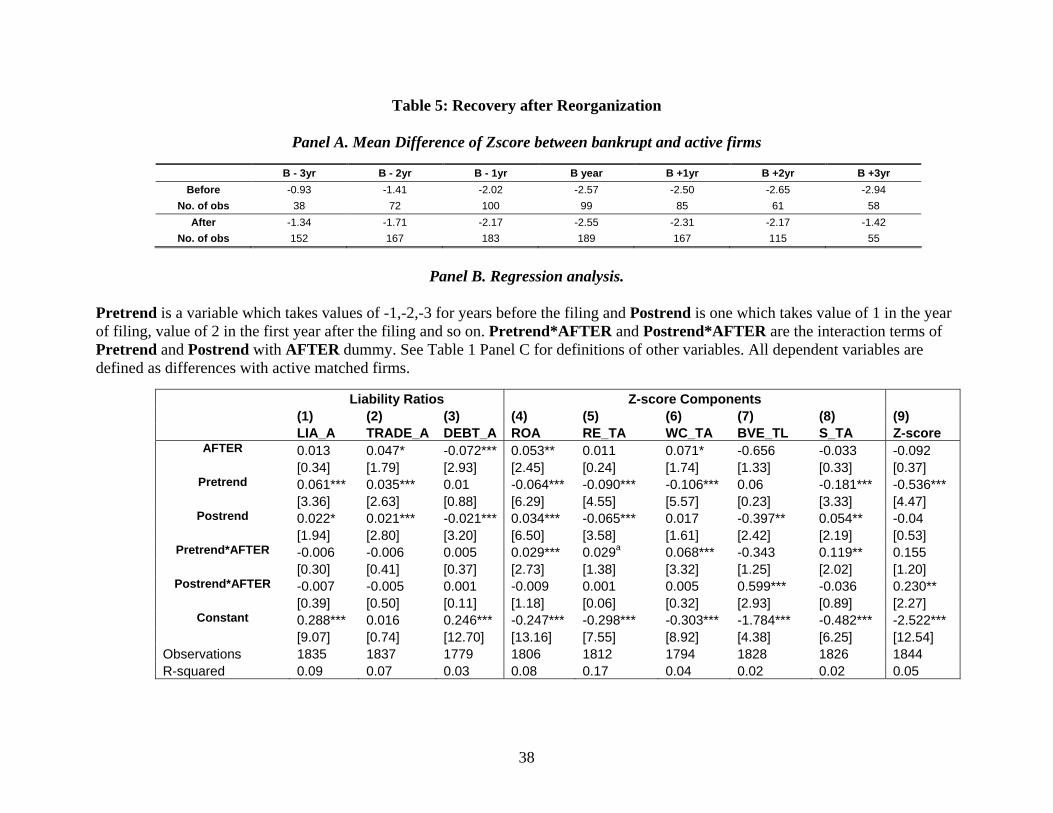
Table 5: Recovery after Reorganization
Panel A. Mean Difference of Zscore between bankrupt and active firms
B - 3yr B - 2yr B - 1yr B year B +1yr B +2yr B +3yr Before -0.93 -1.41 -2.02 -2.57 -2.50 -2.65 -2.94
No. of obs 38 72 100 99 85 61 58 After -1.34 -1.71 -2.17 -2.55 -2.31 -2.17 -1.42
No. of obs 152 167 183 189 167 115 55
Panel B. Regression analysis.
Pretrend is a variable which takes values of -1,-2,-3 for years before the filing and Postrend is one which takes value of 1 in the year of filing, value of 2 in the first year after the filing and so on. Pretrend*AFTER and Postrend*AFTER are the interaction terms of Pretrend and Postrend with AFTER dummy. See Table 1 Panel C for definitions of other variables. All dependent variables are defined as differences with active matched firms.
Liability Ratios Z-score Components (1) (2) (3) (4) (5) (6) (7) (8) (9) LIA_A TRADE_A DEBT_A ROA RE_TA WC_TA BVE_TL S_TA Z-score
AFTER 0.013 0.047* -0.072*** 0.053** 0.011 0.071* -0.656 -0.033 -0.092 [0.34] [1.79] [2.93] [2.45] [0.24] [1.74] [1.33] [0.33] [0.37]
Pretrend 0.061*** 0.035*** 0.01 -0.064*** -0.090*** -0.106*** 0.06 -0.181*** -0.536*** [3.36] [2.63] [0.88] [6.29] [4.55] [5.57] [0.23] [3.33] [4.47]
Postrend 0.022* 0.021*** -0.021*** 0.034*** -0.065*** 0.017 -0.397** 0.054** -0.04 [1.94] [2.80] [3.20] [6.50] [3.58] [1.61] [2.42] [2.19] [0.53]
Pretrend*AFTER -0.006 -0.006 0.005 0.029*** 0.029a 0.068*** -0.343 0.119** 0.155 [0.30] [0.41] [0.37] [2.73] [1.38] [3.32] [1.25] [2.02] [1.20]
Postrend*AFTER -0.007 -0.005 0.001 -0.009 0.001 0.005 0.599*** -0.036 0.230** [0.39] [0.50] [0.11] [1.18] [0.06] [0.32] [2.93] [0.89] [2.27]
Constant 0.288*** 0.016 0.246*** -0.247*** -0.298*** -0.303*** -1.784*** -0.482*** -2.522*** [9.07] [0.74] [12.70] [13.16] [7.55] [8.92] [4.38] [6.25] [12.54] Observations 1835 1837 1779 1806 1812 1794 1828 1826 1844 R-squared 0.09 0.07 0.03 0.08 0.17 0.04 0.02 0.02 0.05
38
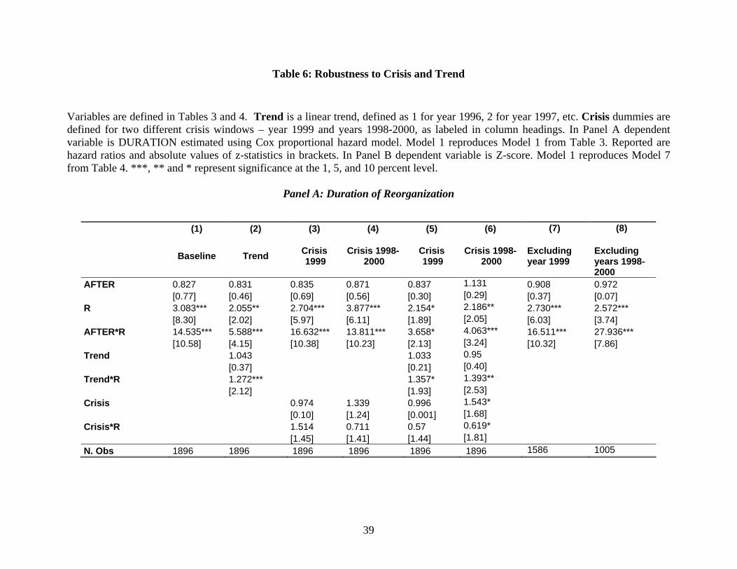
Table 6: Robustness to Crisis and Trend
Variables are defined in Tables 3 and 4. Trend is a linear trend, defined as 1 for year 1996, 2 for year 1997, etc. Crisis dummies are defined for two different crisis windows – year 1999 and years 1998-2000, as labeled in column headings. In Panel A dependent variable is DURATION estimated using Cox proportional hazard model. Model 1 reproduces Model 1 from Table 3. Reported are hazard ratios and absolute values of z-statistics in brackets. In Panel B dependent variable is Z-score. Model 1 reproduces Model 7 from Table 4. ***, ** and * represent significance at the 1, 5, and 10 percent level.
Panel A: Duration of Reorganization
(1) (2) (3) (4) (5) (6) (7) (8)
Baseline Trend Crisis 1999
Crisis 1998-2000
Crisis 1999
Crisis 1998-2000
Excluding year 1999
Excluding years 1998-2000
AFTER 0.827 0.831 0.835 0.871 0.837 1.131 0.908 0.972 [0.77] [0.46] [0.69] [0.56] [0.30] [0.29] [0.37] [0.07] R 3.083*** 2.055** 2.704*** 3.877*** 2.154* 2.186** 2.730*** 2.572*** [8.30] [2.02] [5.97] [6.11] [1.89] [2.05] [6.03] [3.74] AFTER*R 14.535*** 5.588*** 16.632*** 13.811*** 3.658* 4.063*** 16.511*** 27.936*** [10.58] [4.15] [10.38] [10.23] [2.13] [3.24] [10.32] [7.86] Trend 1.043 1.033 0.95 [0.37] [0.21] [0.40] Trend*R 1.272*** 1.357* 1.393** [2.12] [1.93] [2.53] Crisis 0.974 1.339 0.996 1.543* [0.10] [1.24] [0.001] [1.68] Crisis*R 1.514 0.711 0.57 0.619* [1.45] [1.41] [1.44] [1.81] N. Obs 1896 1896 1896 1896 1896 1896 1586 1005
39
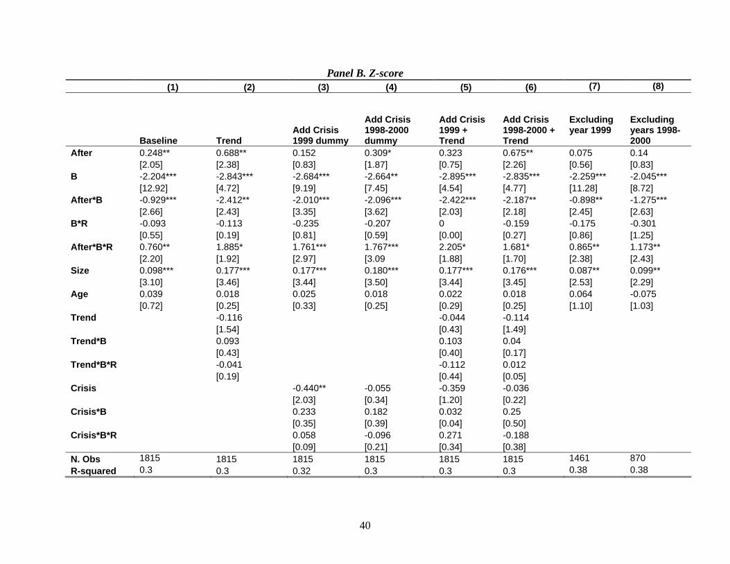
Panel B. Z-score (1) (2) (3) (4) (5) (6) (7) (8)
Baseline Trend Add Crisis 1999 dummy
Add Crisis 1998-2000 dummy
Add Crisis 1999 + Trend
Add Crisis 1998-2000 + Trend
Excluding year 1999
Excluding years 1998-2000
After 0.248** 0.688** 0.152 0.309* 0.323 0.675** 0.075 0.14 [2.05] [2.38] [0.83] [1.87] [0.75] [2.26] [0.56] [0.83] B -2.204*** -2.843*** -2.684*** -2.664** -2.895*** -2.835*** -2.259*** -2.045*** [12.92] [4.72] [9.19] [7.45] [4.54] [4.77] [11.28] [8.72] After*B -0.929*** -2.412** -2.010*** -2.096*** -2.422*** -2.187** -0.898** -1.275*** [2.66] [2.43] [3.35] [3.62] [2.03] [2.18] [2.45] [2.63] B*R -0.093 -0.113 -0.235 -0.207 0 -0.159 -0.175 -0.301 [0.55] [0.19] [0.81] [0.59] [0.00] [0.27] [0.86] [1.25] After*B*R 0.760** 1.885* 1.761*** 1.767*** 2.205* 1.681* 0.865** 1.173** [2.20] [1.92] [2.97] [3.09 [1.88] [1.70] [2.38] [2.43] Size 0.098*** 0.177*** 0.177*** 0.180*** 0.177*** 0.176*** 0.087** 0.099** [3.10] [3.46] [3.44] [3.50] [3.44] [3.45] [2.53] [2.29] Age 0.039 0.018 0.025 0.018 0.022 0.018 0.064 -0.075 [0.72] [0.25] [0.33] [0.25] [0.29] [0.25] [1.10] [1.03] Trend -0.116 -0.044 -0.114 [1.54] [0.43] [1.49] Trend*B 0.093 0.103 0.04 [0.43] [0.40] [0.17] Trend*B*R -0.041 -0.112 0.012 [0.19] [0.44] [0.05] Crisis -0.440** -0.055 -0.359 -0.036 [2.03] [0.34] [1.20] [0.22] Crisis*B 0.233 0.182 0.032 0.25 [0.35] [0.39] [0.04] [0.50] Crisis*B*R 0.058 -0.096 0.271 -0.188 [0.09] [0.21] [0.34] [0.38] N. Obs 1815 1815 1815 1815 1815 1815 1461 870 R-squared 0.3 0.3 0.32 0.3 0.3 0.3 0.38 0.38
40
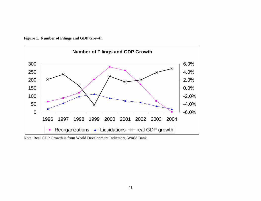
Figure 1. Number of Filings and GDP Growth
Number of Filings and GDP Growth
050
100150200250300
1996 1997 1998 1999 2000 2001 2002 2003 2004-6.0%-4.0%-2.0%0.0%2.0%4.0%6.0%
Reorganizations Liquidations real GDP growth
Note: Real GDP Growth is from World Development Indicators, World Bank.
41
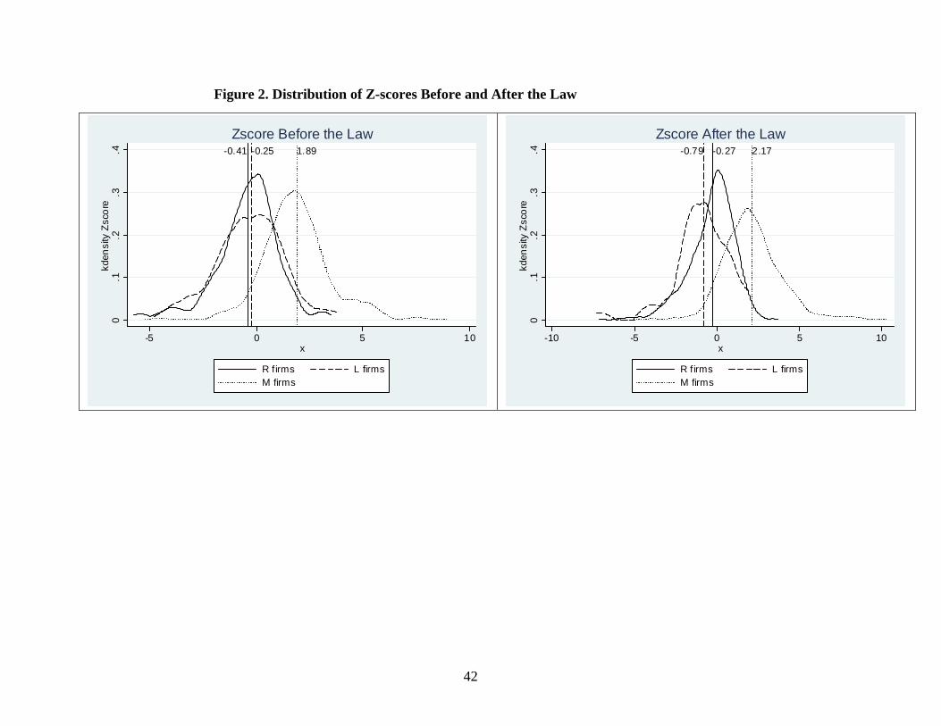
Figure 2. Distribution of Z-scores Before and After the Law
-0.41 -0.25 1.89
0.1
.2.3
.4kd
ensi
ty Z
scor
e
-5 0 5 10x
R firms L firmsM firms
Zscore Before the Law
-0.27-0.79 2.17
0.1
.2.3
.4kd
ensi
ty Z
scor
e
-10 -5 0 5 10x
R firms L firmsM firms
Zscore After the Law
42

-3.50
-3.00
-2.50
-2.00
-1.50
-1.00
-0.50
0.00B -3yr B -2yr B -1yr B B +1yr B +2yr B +3yr
Years before and after bankruptcy
Diff
eren
ces
in Z
scor
e
BeforeAfter
43
Figure 3. Time-series trends before and after the filing