Do State Fiscal Policies Affect State Economic Growth?

Tulane Economics Working Paper Series

Do State Fiscal Policies Affect State Economic Growth?

James AlmDepartment of EconomicsTulane UniversityNew Orleans, [email protected]

Janet RogersDepartment of Planning SectionDivision of Budget & PlanningNevada Department of AdministrationCarson City, [email protected]

Working Paper 1107April 2011

Abstract

What factors influence state economic growth? This paper uses annual state (and local) data for theyears 1947 to 1997 for the 48 contiguous states to estimate the effects of a large number of factors,including taxation and expenditure policies, on state economic growth. A special feature of the empiricalwork is the use of orthogonal distance regression (ODR) to deal with the likely presence of measurementerror in many of the variables. The results indicate that the correlation between state (and state andlocal) taxation policies is often statistically significant but also quite sensitive to the specific regressorset and time period; in contrast, the effects of expenditure policies are much more consistent. Ofsome interest, there is moderately strong evidence that a states political orientation has consistent andmeasurable effects on economic growth; perhaps surprisingly, a more “conservative” political orientationis associated with lower rates of economic growth. Finally, correction for measurement error is essentialin estimating the growth impacts of policies. Indeed, when measurement error is considered via ODRestimation, the estimation results do not support conditional convergence in state per capita income.

Keywords: fiscal policies, regional economic growth, orthogonal distance regressionJEL: H2, H7, O1, O4, R1, R5

Do State Fiscal Policies Affect State Economic Growth?

James Alm and Janet Rogers

Abstract

What factors influence state economic growth? This paper uses annual state (and local) data for the years 1947 to 1997 for the 48 contiguous states to estimate the effects of a large number of factors, including taxation and expenditure policies, on state economic growth. A special feature of the empirical work is the use of orthogonal distance regression (ODR) to deal with the likely presence of measurement error in many of the variables. The results indicate that the correlation between state (and state and local) taxation policies is often statistically significant but also quite sensitive to the specific regressor set and time period; in contrast, the effects of expenditure policies are much more consistent. Of some interest, there is moderately strong evidence that a state’s political orientation has consistent and measurable effects on economic growth; perhaps surprisingly, a more “conservative” political orientation is associated with lower rates of economic growth. Finally, correction for measurement error is essential in estimating the growth impacts of policies. Indeed, when measurement error is considered via ODR estimation, the estimation results do not support conditional convergence in state per capita income. JEL Classification: H2, H7, O1, O4, R1, R5. Keywords: Fiscal Policies, Regional Economic Growth, Orthogonal Distance Regression.

1

1. Introduction

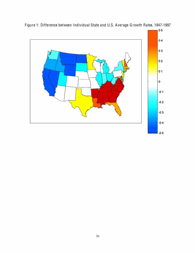
The average annual growth rates of per capita income for the individual 48 contiguous

U.S. states over the last half of the twentieth century range from 1.73 percent to 3.15 percent.

Six states have annual growth rates that exceed the national growth rate by more one-half of a

percentage point at least half the time. Another four states have annual growth rates that are

more than one-half of a percentage point less than the national growth rate at least half the time.

Figure 1 identifies the states with the highest and the lowest average growth rates.

Why is this issue important? In 1947 the median real value of per capita income for the

48 contiguous states was just under $7,500 (in 1997 dollars). If, over the 50 year period from

1947 to 1997 the annual growth rate had been 1.73 percent – the smallest average state growth

rate observed for the period – then the median 1947 value of real per capita income would have

increased to approximately $17,700, or by nearly 235 percent. In contrast, if the annual growth

rate had been 3.15 percent (or the highest observed average growth rate), then this same initial

income would have increased by more than 470 percent, to $35,400. Small changes in growth

rates compound over 50 years to very large differences in per capita incomes. It is therefore

imperative to understand the processes that cause the individual states to show such variations in

their annual growth rates.

Many factors that influence economic growth, such as climate, proximity to national

markets, and energy costs, cannot be changed by state (or national) government policy. Still

other factors like labor force skills can only be changed by government in the long run. This

leaves fiscal policies – tax and expenditures – as one of the primary means (along with

regulations and legal considerations) available to state governments for accelerating economic

growth in the short run.

2

The purpose of this paper is to quantify the effects of various tax and expenditure policies

on state per capita income growth, in order to determine whether there are public policies that

foster higher or lower growth rates. We use annual state (and local) data for the years 1947 to

1997 for the 48 contiguous states to estimate the effects of a wide variety of factors, including

taxation and expenditure policies, on state economic growth. A special feature of our empirical

work is the use of orthogonal distance regression (ODR) to deal with the likely presence of

measurement error in some variables. Our contributions are several: we examine a longer period

of time than most other studies, we include a more comprehensive collection of explanatory

variables, and our use of ODR methods allows us to address the measurement errors that are

inherent in empirical growth studies.

Our results indicate that state economic policies matter, but not always in ways suggested

by some previous work. For example, the correlation between state (and state and local) taxation

policies is often statistically significant but is also quite sensitive to the specific regressor set and

time period. In contrast, the effects of expenditure policies are much more consistent. Of some

interest also, there is moderately strong evidence that a state’s political orientation, as indicated

by such variables as the political party of the governor and the presence of tax and expenditure

limitations, has consistent and measurable effects on per capita income growth rates. Perhaps

surprisingly, a more “conservative” political orientation is associated with lower rates of

economic growth. Finally, although traditional estimation methods suggest conditional

convergence in state per capita income, our ODR results that correct for measurement error do

not support convergence.

3

In the next section we briefly discuss the economic growth literature. In section 3 we

present our empirical strategy, and we also discuss our data. We then discuss our estimation

results. In section 5, we summarize our main results and their implications.

2. A Selective Review of the E conomic G rowth L iterature

Building upon the exogenous growth models of Solow (1956) and Swan (1956), and the

endogenous growth models of Romer (1987, 1990) and Barro and Sala-i-Martin (1992), among

others, there are many empirical studies that attempt to estimate the determinates of economic

growth. Many of these studies examine the growth experience at the country level (e.g., the

“cross-country approach”). Of more relevance here, some work has focused on the growth

experiences of the U.S. states (the “cross-region approach”). See Weil (2005) for a recent survey

of much of this literature.

The standard approach begins by defining the relationship between per capita income in

successive periods as:

ys,t+1 = ys,t (1 + gs,t), (1)

where ys,t is per capita income of state s in period t (and similarly for period t+1) and gs,t is the

growth rate of per capita income of state s over the period t to period t+1. Applying a

logarithmic transformation to equation (1), a linear regression model is obtained as:

gs,t = βx xs,t + εγ s,t , (2)

where xs,t is a vector of explanatory variables for state s in period t (including regional and

geographic characteristics of state s that are constant over time, national characteristics in year t

that do not vary by state, and other variables that vary both by state s and year t), βx is a vector of

4

coefficients, and εγ s,t is the model error term for state s in period t. Equation (2) is then

estimated by various estimation methods, typically ordinary linear least squares (LLS) methods.

Researchers have used a wide range of explanatory variables in their cross-regional

studies. For example, Canto and Webb (1987) present a non-pooled regression of cross-region

annual U.S. data for the period 1957 through 1977. Their independent variable is the average

state growth rate, and explanatory variables include the U.S. growth rate, the difference between

the state’s government purchases and the average of all states’ government purchases, the

difference between the state’s transfer payments and the average of all states’ transfer payments,

and the difference between the state’s relative tax burden and the average of all states’ relative

tax burden. Similarly, Coughlin and Mandelbaum (1989) compare U.S. state per capita incomes

as a percent of average state per capita income and overall state income inequality with regional

variables that indicate coastal, energy-production, sun-belt, and “farm-crises” states. Barro and

Sala-i-Martin (1991) examine cross-region data for the U.S. states using various sub-intervals for

the period 1840 through 1985. They regress the average growth rate against initial income, three

regional specifications (South, Midwest, West), and employment composition for nine industrial

sectors. For some other cross-region studies, see Berry and Kaserman (1987), Mofidi and Stone

(1990), Yu, Wallace, and Nardinelli (1991), Mullen and Williams (1994), and Phillips and Goss

(1995). More recently, Crain and Lee (1999), Caselli and Coleman (2001), Akai and Sakata

(2002), Garofalo and Yamarik (2002), and Tomljanovich (2004), and Holcombe and Lacombe

(2004) conduct similar analyses, with quite mixed results. In perhaps the most comprehensive

work to date, Reed (2008a, 2008b) uses five-year data from 1970 to 1999 for the 48 continental

states, and finds a significant negative relationship between taxes and state economic growth

across a wide range of specifications and estimation procedures.

5

These growth regressions have produced a variety of results, and only modest

consistency. A similar lack of consensus exists in cross-country growth regressions. In a survey

of this latter work, Levine and Renelt (1992) quantify whether the conclusions from cross-

country studies are robust or fragile when there are small changes to the conditioning

information set. Using the extreme bounds analysis of Leamer (1983, 1985), they find that the

estimation results are quite fragile. Sala-i-Martin, Doppelhofer, and Miller (2004) report

somewhat more optimistic results in cross-country studies by examining an approximation to the

cumulative distribution function of the estimators. Even so, their results find that only 18 out of

67 explanatory variables (or only 27 percent) are robustly correlated with measures of economic

growth. Crain and Lee (1999) report similar results for cross-region analysis of U.S. states.

As for the more specific impact of fiscal policies, the generally held presumption is that

higher taxes tend to lower economic growth because of their distortionary effects, because they

tend to discourage the creation of new firms and jobs, and because they inhibit investment. For

example, it is widely held that higher income taxes will lower the rate of growth because they

lower the net return to private investment and make investment activities less attractive. Even

so, there is at least some recognition that the government expenditures financed by tax revenues

might provide superior public services, thereby making a higher-tax area more, not less,

attractive. For example, high public spending on infrastructure investment (e.g., transportation,

communications, education) is generally believed to increase growth rates. Indeed, Mofidi and

Stone (1990) find that state economic performance depends upon the interrelationship between

state taxes and the programs upon which the taxes are spent. They also find that state and local

taxes have a negative effect on growth when the revenues are devoted to transfer payments, but

that expenditures on health, education, and public infrastructure have positive effects on growth.

6

It should also be noted that public sector “institutions” are also likely to affect economic

growth. For example, Persson and Tabellini (1992) outline a theory that relates different

political incentives and political institutions to growth. They conclude that income inequality is

“bad” for growth in democracies, while land concentration is bad for growth everywhere.

Relatedly, there is much empirical work that suggests that factors such as the number of local

governments, the presence of tax and expenditure limitations (TELs), and the political

composition of the governing party affect (and are in turn affected by) fiscal policies.

In sum, existing results for the effects of fiscal policies on state economic growth are

quite variable. The next section presents our approach to estimating the impacts of fiscal (and

other) factors on economic growth.

3. Methods, Data, and Specifications

3.1. Methods

The specification of growth regression models is complicated by the likelihood that the

observed value of per capita income in state s in year t (ys,t) includes an unknown and

unknowable measurement error εy s,t ; that is, εy s,t denotes any random disturbance in the

observed value of per capita income, so that observed ys,t is related to “true” yτs,t by the

relationship:

ys,t = yτs,t + εy s,t, (3)

where the superscript τ denotes the true but unobservable value that excludes all measurement

errors. Consequently, the error term in the resulting growth regression consists of a combination

of the error term associated with the model εγ s,t and the error term associated with the

7

measurement error in per capita income εy s,t (which also includes the measurement error in the

initial period income, or εy s,t0).

The measurement errors in per capita income arise from several sources. First, reliable

measures of price levels or price indices are not always available for individual states for an

extended time period; however, see Berry, Fording, and Hanson (2000). The use of the national

price index, as is employed in all analyses here, could potentially introduce two types of

measurement error: if relative purchasing power parity does not hold across the states, then the

growth rates of real per capita income are mismeasured; and, if absolute purchasing power parity

does not hold, then the levels of real per capita income are mismeasured. Second, per capita

values are computed from population values that are likely measured with error. Third, state

income should be adjusted for the net inflow of the earnings of wage and salary workers who are

interstate commuters, and in this adjustment additional errors are likely introduced.

There is a large econometric literature on measurement errors and the associated errors-

in-variables problem. Work that addresses measurement errors in economic growth regressions

is much sparser (DeLong 1988; Barro and Sala-i-Martin 1991). Ordinary linear or nonlinear

least squares estimation does not address measurement error issues. In contrast, our preferred

estimation method corrects for measurement error, and, in the process, generates significant

improvements in the estimates.

In particular, ordinary least squares methods are inappropriate in the presence of errors-

in-variables. When suitable instruments that are correlated with the explanatory variables but

uncorrelated with the error terms can be found, the method of instrumental variables is often

used when such errors are present. Another procedure is orthogonal distance regression (ODR),

8

which is especially appropriate when the statistical model is nonlinear in the unknown variables

and when there is some information available about the variance of the measurement error

(εy s,t ) (including t0) and the size relative to the model error (εγ s,t). While information about the

variances is not always readily available, it is often reasonable to assume that the standard

deviation of the measurement error is the same for all s and t (including t0), and that the standard

deviation of the model error is also constant over all s and t. Therefore, it is only necessary to

make assumptions about the magnitude of the ratio of the standard deviations to obtain the ODR

solution.

More precisely, if we assume that the measurement error (εy s,t) and the model error

(εγ s,t) in the observation corresponding to state s are independent between observations ti and tj,

for i≠j, and have known (relative) variance, then we can derive the distribution of the combined

error εs=[εy s,t ; εγ s,t] for any state s as Ν (0, Ωε s), where 0 denotes a conformably dimensioned

array of zeros and Ωε s denotes the covariance matrix for all model and measurement errors

associated with state s. As a result, asymptotically maximum likelihood estimators can be

obtained employing ODR. Unlike LLS methods, which minimize the sum of the squared

vertical deviations between the dependent variable and the fitted “line”, ODR methods minimize

the orthogonal (or perpendicular) deviations from the fitted line. See Boggs, Bryd, and Schnabel

(1987) and Boggs, Donaldson, Schnabel, and Spiegelman (1988) for detailed discussions of

ODR methods, including an algorithm that can be used to calculate ODR coefficient estimates.

In fact, we use weighted ODR methods, which allow for heteroscedastic variances within and

between and observations, for nonzero covariances within observations (even though covariances

between observations are identically zero), and for nonlinearity in the explanatory variables

and/or the estimated coefficients.

9

Monte Carlo experiments that we have conducted show that measurement errors do in

fact significantly affect LLS estimates from growth regressions. These experiments also show

that ODR methods noticeably improve bias and mean square error results, even when the

assumptions imposed on the solution are wrong. In particular, the results show that LLS

estimates designed to test the “convergence hypothesis” have a strong tendency to be more

negatively biased than the same coefficient estimated using ODR methods. Furthermore, for all

but one of the more than 80 pairs of median bias examined in our Monte Carlo study, the bias in

the LLS estimator is larger than that in the ODR estimator by more than a factor of 2. These

experiments demonstrate that the measurement errors inherent in growth regression data are

important, and should be considered explicitly when attempting to analyze the factors that affect

economic growth. All of our Monte Carlo results are available upon request.

3.2. Data

Response Variable. The response variable in our basic specifications is the annual

growth rate in per capita personal income for the 48 contiguous states over the period 1947 to

1997. Personal income is computed by the U.S. Department of Commerce Bureau of Economic

Analysis as the sum of wages and salaries, other labor income, proprietors’ income, dividends,

interest, rent, and transfer payments, less personal contributions for social insurance. The main

difference between state personal income and gross state product involves the treatment of

capital income. Personal income includes corporate net income only when individuals receive

payment as dividends; gross state product includes corporate profits and depreciation. Also,

gross state product attributes capital income to the state in which the business activity occurs,

while personal income attributes capital income to the state of the asset holder. Neither measure

includes capital gains.

10

The personal income of a state is defined as the income received by the residents of the

state. However, the estimates of wages and salaries, other labor income, and personal

contributions for social insurance are based mainly on source data that are reported by place of

work, not by place of residence. Accordingly, an adjustment for residence, equal to the net

inflow of the earnings of wage and salary workers who are interstate commuters, must be

estimated so that the place-of-residence measures of earnings and personal income can be

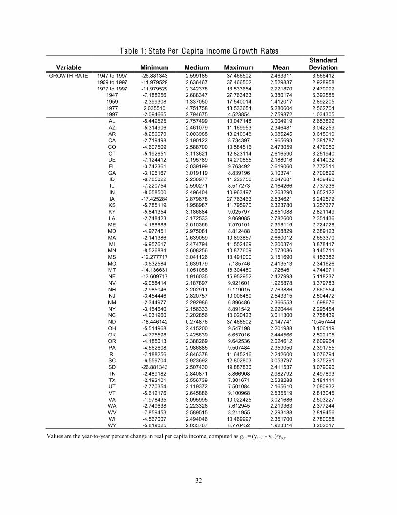
derived. Descriptive statistics for the resulting growth rates in per capita income data are

provided in Table 1.

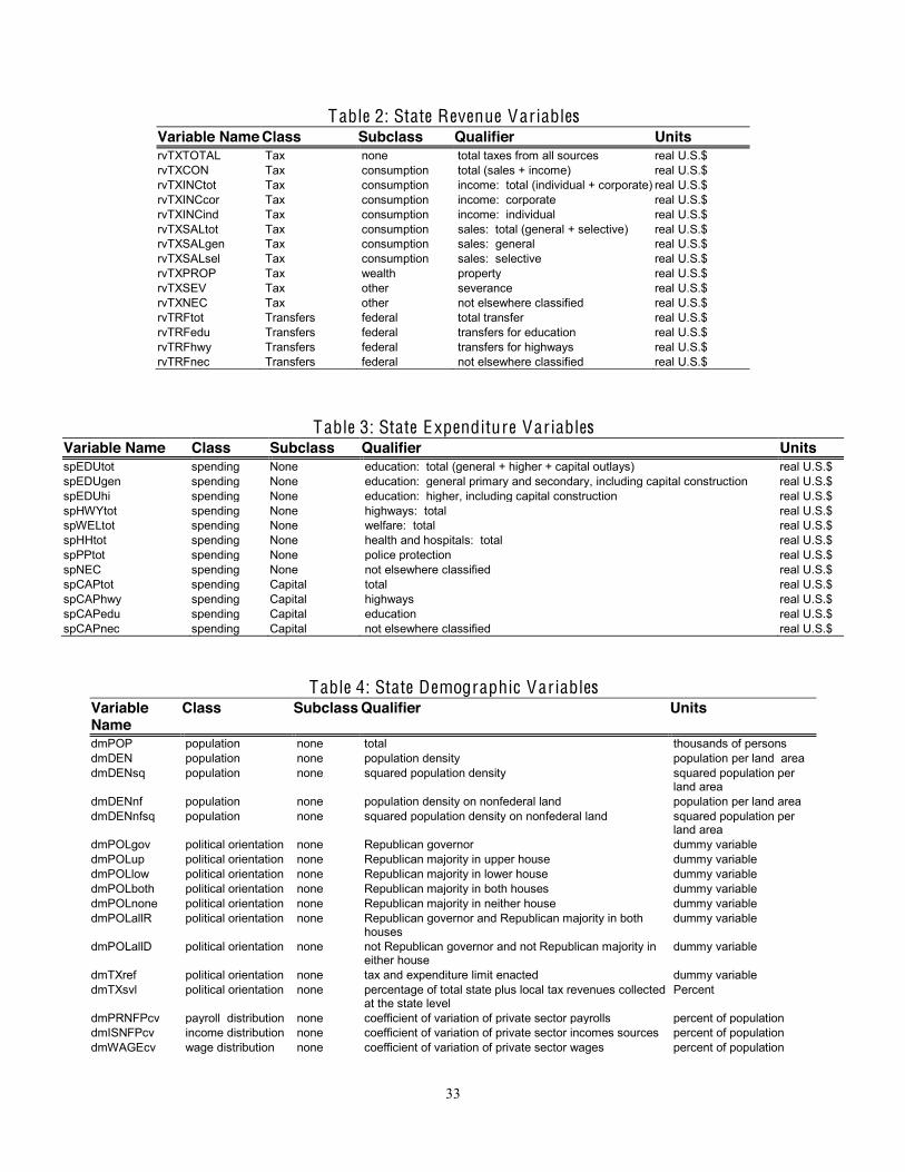
Explanatory Variables. We have assembled more than 130 explanatory variables for

the analysis. These variables can be grouped into five categories: revenues, expenditures,

demographics, geographics, and national. The first three categories include values that vary by

state and by year; the fourth includes values that vary by state but not by year; and the fifth

includes values that vary by year but not by state. All variables in each category are identified in

Tables 2 through 6. Note that the first two letters of each variable name denote the category

(e.g., rv for revenues, sp for spending or expenditures, dm for demographics, ge for geographics,

and us for national).

The revenue and expenditure variables are of obvious interest to policy makers. The

various tax sources (e.g., individual or corporate income, sales, and property taxes) have

implications for the returns to individuals and firms from their activities. Similarly, how a state

chooses to spend these revenues is also important. For example, expenditures on education can

have a direct impact on growth by producing a more capable work force, and are also likely to

have an indirect effect related to the perception of the importance that the state places on

education.

11

The revenue, expenditure, demographic, and geographic variables have been recorded at

a relatively fine level of detail. Composite variables have then been constructed from these

values. For example, the data include values for general and select sales taxes (variables

rvTXSALgen and rvTXSALsel, respectively), as well as total sales taxes (variable rvTXSALtot)

computed from their sum. Similarly, the geographic category includes dummy variables to

indicate natural resources in the state (such as variables geMNau, geMNfe, and geMNcoal), as

well as a dummy variable to indicate the occurrence of one or more of these resources (variable

geMN). The revenue and expenditure variables are included either as per capita values, as a

percent of per capita income, or as a percent of total tax revenue. All explanatory variables are

lagged one year.

Annual values for state revenues and expenditures, as well as for all demographic,

geographic, and national variables, are available for the period 1947 through 1997. Annual

estimates for total state plus local revenues and expenditures are not recorded prior to 1959 (and

not all variables are available until 1977); as a result, our combined state and local analysis is for

the shorter periods 1959 to 1997 (and 1977 to 1997). The data are obtained from various issues

of the Book of the States, the Statistical Abstract of the United States, Current Population

Reports (Series P60), State Government Finances reports, and the World Almanac; some

variables are obtained from personal communication with staff at the U.S. Bureau of the Census.

The primary source for the estimates of total earnings and employment by place of work is the

ES-202 series from the U.S. Bureau of Labor Statistics.

3.3. Specifications

Baseline Regression. Levine and Renelt (1992), Sala-i-Martin (1997), Crain and Lee

(1999), and others have explored the sensitivity of regression results by comparing outcomes

12

against the results from a set of “core” variables. However, there is little agreement on which

variables should be included in the core set of regressors. For example, Levine and Renelt

(1992) use the investment share of gross domestic product (GDP), the initial level of real GDP

per capita, the initial secondary-school enrollment rate, and the average annual rate of population

growth as the core variables in their cross-country analysis. Sala-i-Martin (1997) uses the level

of income, life expectancy, and primary-school enrollment rate as the core variables for his

cross-country sensitivity analysis.

In our work, we choose a set of six core regressors, and our baseline regression (denoted

Regression A) includes only these variables. These core regressors are:

usGRW: the U.S. per capita income growth rate usINF: the U.S. inflation rate usFUELpp: the average U.S. producer price of fuels gePOLstate: a dummy variable equal to 1 if statehood was attained before 1800, and 0

otherwise geREGcon: a dummy variable indicating whether the state is one of the contiguous 48

states (e.g., the constant term in the regression) ys,t0: the value of per capita income for state s in year t0.

These variables are selected for several reasons. The value of per capita income for state s in

year t0 (ys,t0) is typically included in growth regressions to test the convergence hypothesis, or the

notion that a state with a lower initial level of per capita income will experience a higher growth

rate. If states experience convergence, then the sign of the estimated coefficient would be

negative. The geographic variable gePOLstate designates the “age” of the states, old versus

new, and could account for differences in growth rates due to the “maturity” of the state. The

other geographic variable (or geREGcon) is the constant term of the regression.

The remaining three core variables are national variables. The variable usGRW specifies

the annual real U.S. per capita income growth rate. It is well-known that growth equations may

be seriously affected by omitted variables. To the extent that state per capita income growth

13

rates respond to the same shocks and stimuli as the U.S. growth rate, this variable provides some

protection against omitted variable bias. It should also account for much of the business cycle

component of the states’ growth rates. Since individual state economies are small relative to the

U.S. economy as a whole, usGRW is exogenous. Its coefficient is expected to be roughly one.

The regressor usINF is the national inflation rate, and its coefficient is expected to be

negative because inflation is generally presumed to be harmful to economic growth. The

variable usFUELpp, which denotes the average national producer price of fuels, is another

exogenous variable intended to capture the effects of external (fuel) shocks to the U.S. economy.

The baseline regression is estimated for three time periods: 1947 to 1997, 1959 to 1997,

and 1977 to 1997. These correspond, respectively, to the longest period for which annual state

data are available, the longest period for which state plus local total tax and property tax revenue

and state and local expenditure values are available, and the longest period for which all state

plus local tax and expenditure values have been recorded at a relatively fine level of detail. The

results from the baseline regression are presented in Appendix Tables, and are discussed in

section 4. All regressions correct for first order autocorrelation.

Beyond the Baseline Regression. In addition to the baseline regression, several other

primary regression specifications are analyzed for the period 1959 to 1997, using each of three

representations of the fiscal variables (value per capita, value as a percent of income, and value

as a percent of total tax). These other primary specifications are denoted Regression B,

Regression C, and Regression D.

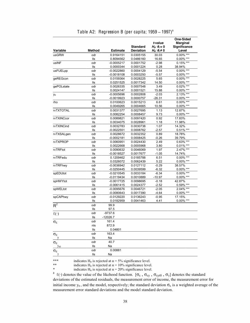
Regression B includes the six core variables plus 12 fiscal variables:

rvTXTOTAL: the sum of all state plus local taxes rvTXINCcor: corporate income tax revenues rvTXINCind: individual income tax revenues (only available at the local level after 1977) rvTXSALgen: state level general sales tax revenues

14

rvTXPROP: the sum of state plus local property taxes rvTRFtot: the total amount of revenues transferred from the federal to the state

government rvTRFedu: the amount of revenues earmarked for education that are transferred from the

federal to the state government rvTRFhwy: the amount of revenues earmarked for highways that are transferred from the

federal to the state government spEDUtot: the sum of state plus local expenditures for primary and secondary education,

including capital construction spHWYtot: the sum of state plus local expenditures for highways, including capital

construction spWELtot: the sum of state plus local expenditures for welfare spCAPhwy: the sum of state plus local expenditures for capital construction of highways.

(Remember that many of the tax variables are not available at the local level prior to 1977.) This

set of variables is assembled to examine the impact of tax, transfer, general expenditure, and

capital outlay variables. See Tables 2 and 3 for variable definitions.

Regression C includes the six core variables from Regression A plus the 12 fiscal

variables included in Regression B, along with another 30 variables from the demographic,

geographic, and national variable sets. This set of variables includes every variable in which

anyone might reasonably have any interest, plus a few others thrown in for good measure. These

variables are defined in Tables 4, 5, and 6.

Regression D represents a subset of variables used in Regression C. It includes the 12

fiscal variables from Regression B, plus 13 variables selected on the basis of their explanatory

power. These 13 variables are: dmPOLgov, dmTXref, dmTXsvl, dmPOP, dmDEN, dmWAGEcv,

dmPRNFPcv, geHEtotP, geSIZ, geSIZPf, geREGatl, geREGpac, and gePOLCgov. We believe

that this variable set is the most representative, and it is the one discussed in greatest detail in

section 4.

Finally, we have also estimated a wide variety of additional specifications. Regression E

uses the same regressors and time spans as Regression D, but excludes the five states with the

15

highest variability of growth rates (Iowa, Montana, Nebraska, North Dakota, and South Dakota).

Regression F has the same explanatory variables and uses the same subset of states as

Regression E , but the time span is 1977 to 1996 rather than 1959 to 1996. Regression G is the

same as Regression F , except that total state plus local fiscal values are used for all tax and

expenditure variables. We discuss summary results for these specifications later.

Aside from these specifications, it should be noted that we have estimated many

additional specifications, including ones in which we examine alternative time periods, in which

we include state plus local measures of all tax and expenditure variables, in which dummy

variables for the presence (or absence) of specific tax instruments are used rather than their

values, and in which the growth experience of two individual states (Colorado and Georgia) are

examined separately. All results are available upon request.

4. Results

Estimation results from some basic specifications are presented in Appendix Tables A1 to

A7; all other results are available upon request. The boxes included below summarize the

outcomes from the regressions. Column headings within the boxes indicate the time period, the

fiscal variable parameterization (e.g., per capita, percent of income, percent of total taxes), as

well as the regression identifier (e.g., A, B, C, D, E , F , or G). The row headings indicate the

construction of the fiscal variables: “asl” denotes that all fiscal variables are constructed using

the sum of state plus local amounts, “psl” denotes that property taxes, total taxes, and

expenditures values are constructed using the sum of state plus local amounts (while other

revenue variables are composed of only state values), and “s” denotes that fiscal values are

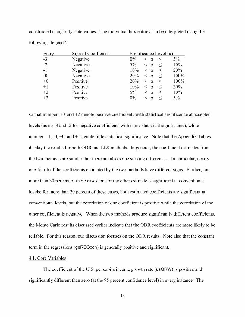
16

constructed using only state values. The individual box entries can be interpreted using the

following “legend”:

Entry Sign of Coefficient Significance Level (α)_____ -3 Negative 0% < α ≤ 5% -2 Negative 5% < α ≤ 10% -1 Negative 10% < α ≤ 20% -0 Negative 20% < α ≤ 100% +0 Positive 20% < α ≤ 100% +1 Positive 10% < α ≤ 20% +2 Positive 5% < α ≤ 10% +3 Positive 0% < α ≤ 5%

so that numbers +3 and +2 denote positive coefficients with statistical significance at accepted

levels (as do -3 and -2 for negative coefficients with some statistical significance), while

numbers -1, -0, +0, and +1 denote little statistical significance. Note that the Appendix Tables

display the results for both ODR and LLS methods. In general, the coefficient estimates from

the two methods are similar, but there are also some striking differences. In particular, nearly

one-fourth of the coefficients estimated by the two methods have different signs. Further, for

more than 30 percent of these cases, one or the other estimate is significant at conventional

levels; for more than 20 percent of these cases, both estimated coefficients are significant at

conventional levels, but the correlation of one coefficient is positive while the correlation of the

other coefficient is negative. When the two methods produce significantly different coefficients,

the Monte Carlo results discussed earlier indicate that the ODR coefficients are more likely to be

reliable. For this reason, our discussion focuses on the ODR results. Note also that the constant

term in the regressions (geREGcon) is generally positive and significant.

4.1. Core Variables

The coefficient of the U.S. per capita income growth rate (usGRW) is positive and

significantly different than zero (at the 95 percent confidence level) in every instance. The

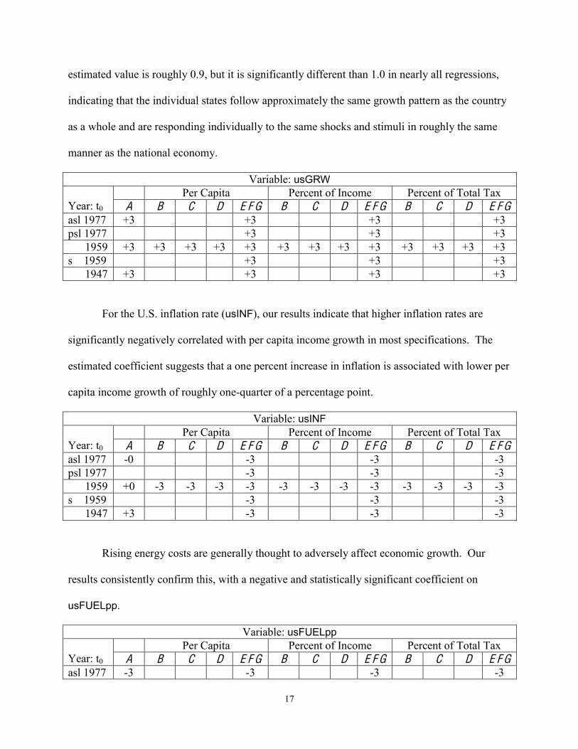
17

estimated value is roughly 0.9, but it is significantly different than 1.0 in nearly all regressions,

indicating that the individual states follow approximately the same growth pattern as the country

as a whole and are responding individually to the same shocks and stimuli in roughly the same

manner as the national economy.

Variable: usGRW Year: t0

Per Capita Percent of Income Percent of Total Tax A B C D E F G B C D E F G B C D E F G

asl 1977 +3 +3 +3 +3 psl 1977 +3 +3 +3 1959 +3 +3 +3 +3 +3 +3 +3 +3 +3 +3 +3 +3 +3 s 1959 +3 +3 +3 1947 +3 +3 +3 +3

For the U.S. inflation rate (usINF), our results indicate that higher inflation rates are

significantly negatively correlated with per capita income growth in most specifications. The

estimated coefficient suggests that a one percent increase in inflation is associated with lower per

capita income growth of roughly one-quarter of a percentage point.

Variable: usINF Year: t0


asl 1977 -0 -3 -3 -3 psl 1977 -3 -3 -3 1959 +0 -3 -3 -3 -3 -3 -3 -3 -3 -3 -3 -3 -3 s 1959 -3 -3 -3 1947 +3 -3 -3 -3

Rising energy costs are generally thought to adversely affect economic growth. Our

results consistently confirm this, with a negative and statistically significant coefficient on

usFUELpp.

Variable: usFUELpp Year: t0


asl 1977 -3 -3 -3 -3

18

psl 1977 -3 -3 -3 1959 -3 -3 -3 -3 -3 -3 -3 -3 -3 -3 -3 -3 -3 s 1959 -3 -3 -3 1947 -3 -3 -3 -3

The dummy variable gePOLstate provides a simple designation of the “age” of the state,

as determined by the year in which statehood was obtained. Values of 1 for gePOLstate identify

states that acquired statehood prior to 1800 (e.g., “old” states), while values of 0 identify states

that acquired statehood after 1800 (e.g., “young” states). The estimated coefficient for

gePOLstate is always positive and statistically significant, indicating that older states have

higher per capita income growth than younger states. This is a plausible result, and is consistent

with the presence of more developed infrastructures in older states. However, this result is not

consistent with convergence.

Variable: gePOLstate Year: t0


asl 1977 +3 +3 +3 +3 psl 1977 +3 +3 +3 1959 +3 +3 +3 +3 +3 +3 +3 +3 +3 +3 +3 +3 +3 s 1959 +3 +3 +3 1947 +3 +3 +3 +3

The neoclassical growth model asserts that, ceteris paribus, an economy with a lower

initial income will grow faster than an economy with a higher initial income. However, in our

results, initial income (ys,t0) has quite variable effects on the various specifications. When the

explanatory variables include the full set of socio-economic regressors, our results provide little

support for conditional convergence, and strong evidence of divergence after 1977.

When the coefficient on ys,t0 is not significant at conventional levels, it might be argued

that multicollinearity among the regressors is the problem. However, variance decomposition

19

results indicate that this is unlikely. Moreover, our Monte Carlo experiments indicate that the

measurement errors in per capita income have a significant and adverse effect on LLS results

when annual data are employed. However, if annual data are not used, then the fiscal and policy

variables that are being examined must be aggregated over the period between observations to

obtain a single representative value, even though it is the effect of the variation of these fiscal

and policy variables that we are seeking to measure. Hence, previously reported results of

convergence are suspect either because they have not taken measurement errors into account, or

because the fiscal and policy variables have been recorded in such a way that their effect on

economic growth cannot be accurately determined. The ODR results reported here suffer from

neither of these problems.

Variable: ys,to Year: t0


asl 1977 -0 +3 +3 +3 psl 1977 +3 +3 +3 1959 -3 -3 +3 +3 +3 -3 +0 +0 +0 -3 -0 +0 +0 s 1959 -0 -0 -0 1947 -3 +0 -1 -0

In sum, the analysis of the core variables identifies strong correlations where they are

expected. The only surprising result is that for initial income, which indicates divergence from

1977 to the present.

4.2. Fiscal Variables

The variable rvTXTOTAL (expressed as real dollars per capita or as a percent of total state

income) includes all tax revenues but excludes transfers from the federal government. The

estimated coefficient on rvTXTOTAL is quite sensitive to the other variables that are included and

also to the specific measures of tax and other fiscal variables; in additional specifications that are

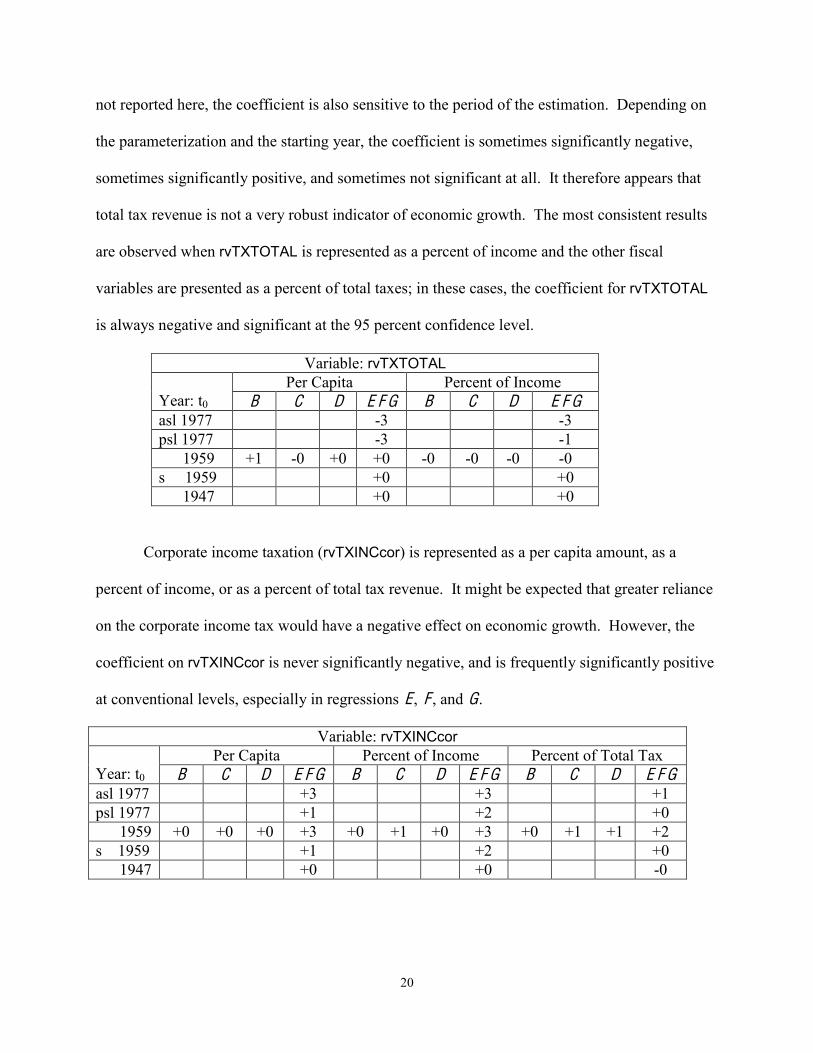
20

not reported here, the coefficient is also sensitive to the period of the estimation. Depending on

the parameterization and the starting year, the coefficient is sometimes significantly negative,

sometimes significantly positive, and sometimes not significant at all. It therefore appears that

total tax revenue is not a very robust indicator of economic growth. The most consistent results

are observed when rvTXTOTAL is represented as a percent of income and the other fiscal

variables are presented as a percent of total taxes; in these cases, the coefficient for rvTXTOTAL

is always negative and significant at the 95 percent confidence level.

Variable: rvTXTOTAL Year: t0

Per Capita Percent of Income B C D E F G B C D E F G

asl 1977 -3 -3 psl 1977 -3 -1 1959 +1 -0 +0 +0 -0 -0 -0 -0 s 1959 +0 +0 1947 +0 +0

Corporate income taxation (rvTXINCcor) is represented as a per capita amount, as a

percent of income, or as a percent of total tax revenue. It might be expected that greater reliance

on the corporate income tax would have a negative effect on economic growth. However, the

coefficient on rvTXINCcor is never significantly negative, and is frequently significantly positive

at conventional levels, especially in regressions E , F , and G.

Variable: rvTXINCcor Year: t0

Per Capita Percent of Income Percent of Total Tax B C D E F G B C D E F G B C D E F G

asl 1977 +3 +3 +1 psl 1977 +1 +2 +0 1959 +0 +0 +0 +3 +0 +1 +0 +3 +0 +1 +1 +2 s 1959 +1 +2 +0 1947 +0 +0 -0

21

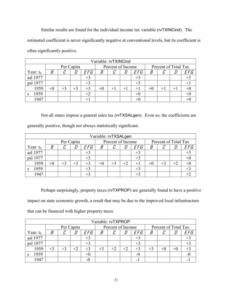
Similar results are found for the individual income tax variable (rvTXINCind). The

estimated coefficient is never significantly negative at conventional levels, but its coefficient is

often significantly positive.

Variable: rvTXINCind Year: t0


asl 1977 +3 +3 +3 psl 1977 +3 +3 +1 1959 +0 +3 +3 +3 +0 +1 +1 +1 +0 +1 +1 +0 s 1959 +2 +0 +0 1947 +1 +0 +0

Not all states impose a general sales tax (rvTXSALgen). Even so, the coefficients are

generally positive, though not always statistically significant.

Variable: rvTXSALgen Year: t0


asl 1977 +3 +3 +3 psl 1977 +3 +3 +0 1959 +0 +3 +3 +3 +0 +3 +2 +1 +0 +3 +2 +0 s 1959 +3 +3 +3 1947 +3 +3 +2

Perhaps surprisingly, property taxes (rvTXPROP) are generally found to have a positive

impact on state economic growth, a result that may be due to the improved local infrastructure

that can be financed with higher property taxes.

Variable: rvTXPROP Year: t0


asl 1977 +3 +3 +3 psl 1977 +3 +3 +3 1959 +3 +3 +2 +3 +3 +2 +2 +3 +3 +0 +0 +3 s 1959 +0 -0 -0 1947 -0 -1 -1

22

The coefficient on total transfers from the federal government (rvTRFtot) is always

positive, and generally significantly so.

Variable: rvTRFtot Year: t0


asl 1977 +3 +3 +3 psl 1977 +3 +3 +3 1959 +2 +3 +3 +3 +0 +2 +1 +3 +1 +3 +2 +0 s 1959 +3 +3 +3 1947 +3 +2 +3

Similarly, federal transfers for education (rvTRFedu) are significantly and positively

correlated with income growth in all instances. The magnitude of coefficient indicates that each

additional one dollar in per capita transfers is associated with an increase in per capita income

growth rates by one-hundredth of a percentage point.

Variable: rvTRFedu Year: t0


asl 1977 +3 +3 +3 psl 1977 +3 +3 +3 1959 +3 +3 +3 +3 +3 +3 +3 +3 +3 +3 +3 +3 s 1959 +3 +3 +3 1947 +3 +3 +3

In contrast, federal transfers for highways (rvTRFhwy) are not consistently related to

economic growth. Depending on the specification, the estimated coefficient is sometimes

positive and significant, sometimes negative and significant, and sometimes insignificant. The

negative relationship between highway transfers and growth is most pronounced after 1977,

perhaps due to the need for state matching funds. Also, there are likely to be long lags associated

with any benefits from highway construction.

Variable: rvTRFhwy Per Capita Percent of Income Percent of Total Tax

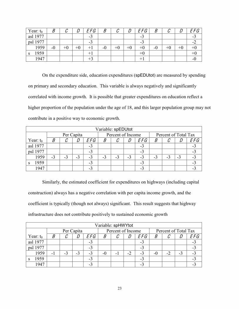
23

Year: t0 B C D E F G B C D E F G B C D E F G asl 1977 -3 -3 -3 psl 1977 -3 -3 -2 1959 -0 +0 +0 +1 -0 +0 +0 +0 -0 +0 +0 +0 s 1959 +1 +0 +0 1947 +3 +1 -0

On the expenditure side, education expenditures (spEDUtot) are measured by spending

on primary and secondary education. This variable is always negatively and significantly

correlated with income growth. It is possible that greater expenditures on education reflect a

higher proportion of the population under the age of 18, and this larger population group may not

contribute in a positive way to economic growth.

Variable: spEDUtot Year: t0


asl 1977 -3 -3 -3 psl 1977 -3 -3 -3 1959 -3 -3 -3 -3 -3 -3 -3 -3 -3 -3 -3 -3 s 1959 -3 -3 -3 1947 -3 -3 -3

Similarly, the estimated coefficient for expenditures on highways (including capital

construction) always has a negative correlation with per capita income growth, and the

coefficient is typically (though not always) significant. This result suggests that highway

infrastructure does not contribute positively to sustained economic growth

Variable: spHWYtot Year: t0


asl 1977 -3 -3 -3 psl 1977 -3 -3 -3 1959 -1 -3 -3 -3 -0 -1 -2 -3 -0 -2 -3 -3 s 1959 -3 -3 -3 1947 -3 -3 -3

24

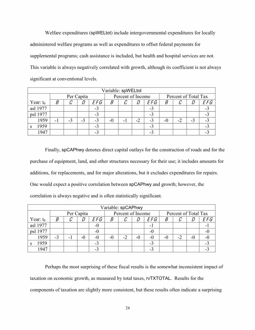
Welfare expenditures (spWELtot) include intergovernmental expenditures for locally

administered welfare programs as well as expenditures to offset federal payments for

supplemental programs; cash assistance is included, but health and hospital services are not.

This variable is always negatively correlated with growth, although its coefficient is not always

significant at conventional levels.

Variable: spWELtot Year: t0


asl 1977 -3 -3 -3 psl 1977 -3 -3 -3 1959 -1 -3 -3 -3 -0 -1 -2 -3 -0 -2 -3 -3 s 1959 -3 -3 -3 1947 -3 -3 -3

Finally, spCAPhwy denotes direct capital outlays for the construction of roads and for the

purchase of equipment, land, and other structures necessary for their use; it includes amounts for

additions, for replacements, and for major alterations, but it excludes expenditures for repairs.

One would expect a positive correlation between spCAPhwy and growth; however, the

correlation is always negative and is often statistically significant.

Variable: spCAPhwy Year: t0


asl 1977 -0 -1 -1 psl 1977 -0 -0 -0 1959 -3 -1 -0 -0 -0 -2 -0 -0 -0 -2 -0 -0 s 1959 -3 -3 -3 1947 -3 -3 -3

Perhaps the most surprising of these fiscal results is the somewhat inconsistent impact of

taxation on economic growth, as measured by total taxes, rvTXTOTAL. Results for the

components of taxation are slightly more consistent, but these results often indicate a surprising

25

positive (though often statistically insignificant) impact of taxes on growth. Also, transfers (in

total and for education) typically have a positive and significant impact on growth, while

transfers for highways generate mixed results. Indeed, the expenditure results are considerably

more consistent than the tax results. In almost all cases, expenditures are negatively and

significantly correlated with growth in per capita income, even spending that augments state

infrastructure.

4.3. Socio-economic, Demographic, Geographic, and Political Variables

We have also included many other variables in various specifications. We do not discuss

all of these results in detail, but it is useful to highlight some of the more provocative findings.

One political variable is a dummy variable that equals 1 if the governor of the state (in

the previous year) is Republican and 0 otherwise (dmPOLgov). It is widely believed that

Republicans are more sympathetic to, and more encouraging of, policies that generate economic

growth. However, the estimated coefficient on dmPOLgov is always negative and often

significantly so.

Similarly, we include a dummy variable equal to 1 if the state has a TEL in place (on

either the tax or the expenditure side) and 0 otherwise (dmTXREF). It might be expected that

such limitations increase growth by placing limits on the size and the reach of government; in

contrast, a TEL might lead to reductions in government infrastructure and service spending,

thereby reducing growth. In fact, we find that the coefficient on dmTXREF is always negative,

though not always statistically significant. Regressions F and G, which cover the period from

1977 to 1996 and which exclude the five high volatility states, indicate that passage of a TEL

reduces per capita income growth by about three tenths of a percentage point.

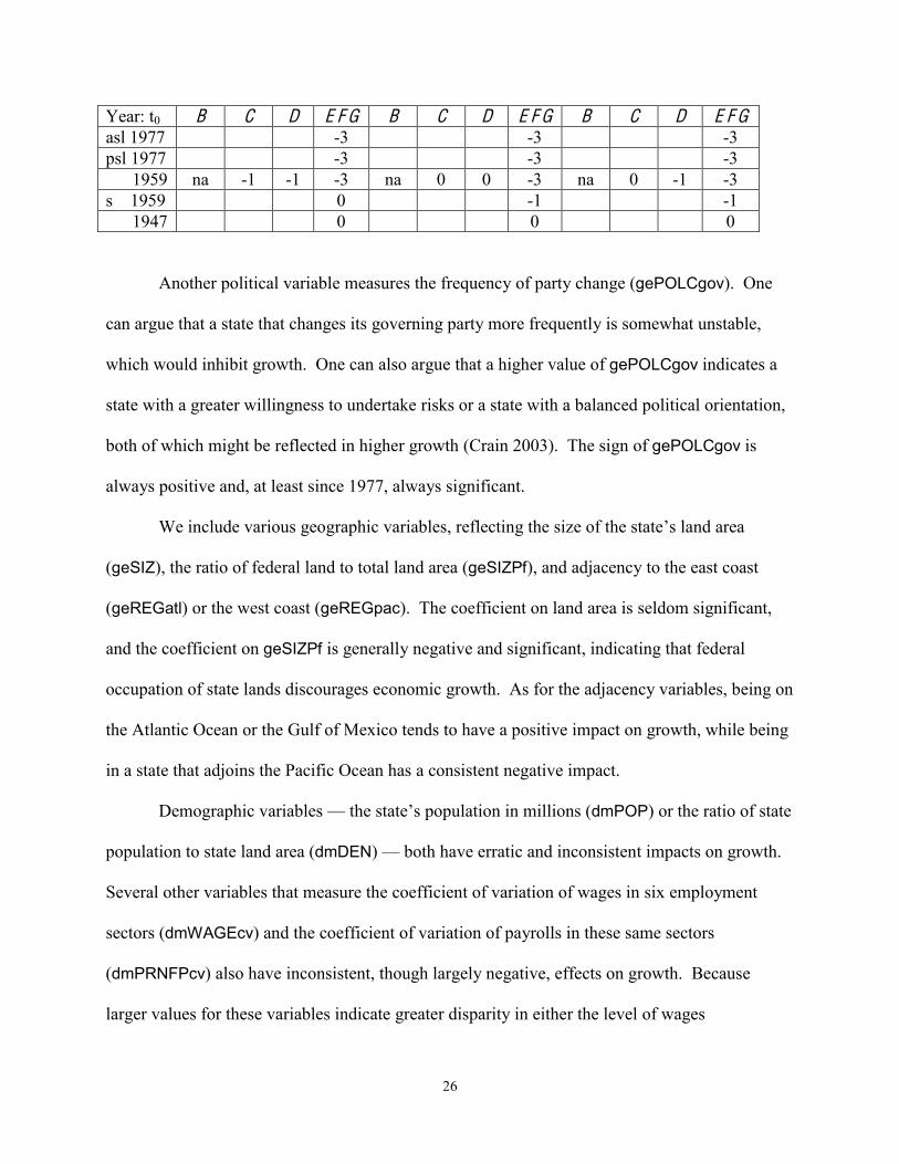
Variable: dmTAXref Per Capita Percent of Income Percent of Total Tax

26

Year: t0 B C D E F G B C D E F G B C D E F G asl 1977 -3 -3 -3 psl 1977 -3 -3 -3 1959 na -1 -1 -3 na 0 0 -3 na 0 -1 -3 s 1959 0 -1 -1 1947 0 0 0

Another political variable measures the frequency of party change (gePOLCgov). One

can argue that a state that changes its governing party more frequently is somewhat unstable,

which would inhibit growth. One can also argue that a higher value of gePOLCgov indicates a

state with a greater willingness to undertake risks or a state with a balanced political orientation,

both of which might be reflected in higher growth (Crain 2003). The sign of gePOLCgov is

always positive and, at least since 1977, always significant.

We include various geographic variables, reflecting the size of the state’s land area

(geSIZ), the ratio of federal land to total land area (geSIZPf), and adjacency to the east coast

(geREGatl) or the west coast (geREGpac). The coefficient on land area is seldom significant,

and the coefficient on geSIZPf is generally negative and significant, indicating that federal

occupation of state lands discourages economic growth. As for the adjacency variables, being on

the Atlantic Ocean or the Gulf of Mexico tends to have a positive impact on growth, while being

in a state that adjoins the Pacific Ocean has a consistent negative impact.

Demographic variables — the state’s population in millions (dmPOP) or the ratio of state

population to state land area (dmDEN) — both have erratic and inconsistent impacts on growth.

Several other variables that measure the coefficient of variation of wages in six employment

sectors (dmWAGEcv) and the coefficient of variation of payrolls in these same sectors

(dmPRNFPcv) also have inconsistent, though largely negative, effects on growth. Because

larger values for these variables indicate greater disparity in either the level of wages

27

(dmWAGEcv) or the level of employment (dmPRNFPcv) in these sectors, the negative

coefficients on these variables suggest that the concentration of a state’s employment base in

fewer sectors has a positive effect on growth.

Overall, these different results tend to be somewhat more robust than those for the fiscal

variables (especially the tax variables).

5. Conclusions

This paper reports the results of an empirical analysis of economic growth in the United

States for the years 1947 through 1997, presenting empirical results against which theoretical

models of economic growth can be compared. The analysis uses annual data to examine the

effects of government policy variables at the state and local levels, as well as the effects of a

wide range of other socio-economic, demographic, geographic, and political variables.

The empirical literature on economic growth includes hundreds of articles examining the

growth effects of a multitude of variables. Our paper differs from these studies in several

important ways: it examines annual data over a longer period than most other studies, it includes

a much more comprehensive collection of explanatory variables, and it addresses the

measurement errors inherent in per capita income data.

Several main conclusions emerge.

First, our estimation results indicate that a state’s fiscal policies have a measurable

relationship with per capita income growth, although not always in the expected direction and

seldom in a way that is robust to alternative specifications. Tax impacts on state economic

growth are quite variable; expenditure impacts are more consistent across different

specifications. The statistically significant correlation between state (and state plus local) total

28

tax revenues and economic growth is very sensitive to the regressor set and the time period

examined. Often, there are highly significant correlations measured between these variables and

per capita income growth, but further work needs to be done before it can be determined what

these results mean.

Second, there is strong evidence that a state’s political orientation, as indicated by

whether the governor is Republican or Democrat, whether the state has enacted tax and

expenditure limitation legislation, and whether the state frequently elects a governor of the same

party as the incumbent, have consistent, measurable, and significant effects on economic growth.

Perhaps surprisingly, having a Republican governor is associated with lower rates of growth.

Third, the methods commonly employed for growth regression analyses could be

inadequate and could adversely affect the results because most previously reported results have

not taken measurement errors into account. Again, we do not discuss these results in detail here,

but we have some evidence that it is very likely that measurement errors have had a significant

impact on previously reported growth regression results, especially with regards to convergence.

Indeed, although ordinary linear least squares estimates suggest that there is conditional

convergence in per capita income across the 48 contiguous states, our ODR estimates indicate

strong evidence of divergence.

References

Akai, Nobuo and Masayo Sakata. 2002. Fiscal Decentralization Contributes to Economic Growth: Evidence from State-level Cross-section Data for the United States. Journal of Urban Economics 52 (1): 93–108. Barro, Robert J. and Xavier Sala-i-Martin. 1991. Convergence across States and Regions. Brookings Papers on Economic Activity 1 (1): 107–182.

29

Barro, Robert J. and Xavier and Sala-i-Martin. 1992. Convergence. The Journal of Political Economy 100 (2): 223–251. Barro, Robert J. and Xavier Sala-i-Martin. 1992. Public Finance in Models of Economic Growth. Review of Economic Studies 59 (4): 645–661. Berry, Dan L. and David L. Kaserman. 1987. A Diffusion Model of Long-run State Economic Development. Atlantic Economic Journal 21 (4): 39-54. Berry, William D., Richard C. Fording, and Russell L. Hanson. 2000. An annual cost of living index for the American states, 1960-1995. The Journal of Politics 62 (2): 550-567. Boggs, Paul T., Richard H. Byrd, and Robert B. Schnabel. 1987. A Stable and Efficient Algorithm for Nonlinear Orthogonal Distance Regression. Society for Industrial and Applied Mathematics (SIAM) Journal of Scientific and Statistical Computing 8 (6): 1052-1078. Boggs, Paul T., Janet Rogers Donaldson, Robert B. Schnabel, and Clifford H. Spiegelman. 1988. A Computational Examination of Orthogonal Distance Regression. Journal of Econometrics 38 (1/2): 169-201. Canto, Victor and Robert I. Webb. 1987. The Effect of State Fiscal Policy on State Relative Economic Performance. Southern Economic Journal 54 (1): 186–202. Caselli, Francesco and Wilbur John Coleman II. 2001. The U.S. Structural Transformation and Regional Convergence: A Reinterpretation. The Journal of Political Economy 109 (3): 584-616. Coughlin, Cletus C. and Thomas B. Mandelbaum. 1989. Have Federal Spending and Taxation Contributed to the Divergence of State Per Capita Incomes in the 1980s? Federal Reserve Bank of St. Louis Review 71 (4): 29-42. Crain, W. Mark and Katherine J. Lee. 1999. Economic Growth Regressions for the American States: A Sensitivity Analysis. Economic Inquiry 37 (2): 242-257. Crain, W. Mark. 2003. Volatile States: Institutions, Policy, and the Performance of American State Economies. Ann Arbor, MI: The University of Michigan Press. De Long, J. Bradford. 1988. Productivity Growth, Convergence, and Welfare: Comment. The American Economic Review 78 (5): 1138-1154. Garofalo, Gasper A. and Steven Yamarik. 2002. Regional Convergence: Evidence from a New State-by-state Capital Stock Series. The Review of Economics and Statistics 84 (2): 316-323. Holcombe, Randall G. and Donald J. Lacombe. 2004. The Effect of State Income Taxation on Per Capita Income Growth. Public F inance Review 32 (3): 292-312.

30

Leamer, Edward E. 1983. Let’s Take the Con Out of Econometrics. The American Economic Review 73 (1): 31-43. Leamer, Edward E. 1985. Sensitivity Analysis Would Help. The American Economic Review 75 (3): 308-313. Levine, Ross and David Renelt. 1992. A Sensitivity Analysis of Cross-country Growth Regressions. The American Economic Review 82 (4): 942–963. Mofidi, Alaeddin and Joe A. Stone. 1990. Do State and Local Taxes Affect Economic Growth? The Review of Economics and Statistics 72 (4): 686–691. Mullen, John K. and Martin Williams. 1994. Marginal Tax Rates and State Economic Growth. Regional Science and Urban Economics 24 (6): 687-705. Persson, Torsten and Guido Tabellini. 1992. Growth, Distribution, and Politics. European Economic Review 36 (2-3): 593-602. Phillips, Joseph M. and Ernest P. Goss. 1995. The Effect of State and Local Taxes on Economic Development: A Meta-analysis. Southern Economic Journal 62 (2): 320–333. Reed, W. Robert. 2008a. The Robust Relationship between Taxes and U. S. State Income Growth. National Tax Journal 61 (1): 57-80. Reed, W. Robert. 2008b. The Determinants of U.S. State Economic Growth: A Less Extreme Bounds Analysis. Economic Inquiry 47 (4): 685-700. Romer, Paul M. 1987. Growth Based on Increasing Returns due to Specialization. The American Economic Review 77 (2): 56–62. Romer, Paul M. 1990. Endogenous Technological Change. The Journal of Political Economy 98 (5, Part 2): S71–S102. Sala-i-Martin, Xavier. 1997. I Just Ran Two Million Regressions. The American Economic Review, Papers and Proceedings of the American Economic Association 87 (2): 178–183. Sala-i-Martin, Xavier, Gernot Doppelhofer, and Ronald I. Miller. 2004. Determinants of Long-term Growth: A Bayesian Averaging of Classical Estimates (BACE) Approach. The American Economic Review 94 (4): 813-835. Solow, Robert M. 1956. A Contribution to the Theory of Economic Growth. The Quarterly Journal of Economics 70 (1): 65–94. Swan, Trevor W. 1956. Economic Growth and Capital Accumulation. Economic Record 32: 334–361.

31

Tomljanovich, Marc. 2004. The Role of State Fiscal Policy in State Economic Growth. Contemporary Economic Policy 22 (3): 318-330. Weil, David N. 2005. Economic Growth. Boston, MA: Pearson Education, Inc. and Addison-Wesley. Author Biographies James Alm is a professor of economics at Tulane University. Much of his research has examined the responses of individuals and firms to taxation, in such areas as tax compliance and tax evasion, the income tax treatment of the family, tax reform, social security, housing, and indexation. He has also worked extensively on fiscal reform projects overseas. Janet Rogers received her Ph.D. in economics from the University of Colorado at Boulder, and has worked extensively on state and local fiscal issues. She currently is the Chief State Economist for the Department of Administration, Division of Budget and Planning, for the State of Nevada. Previously, she was the Senior Economist for the State of Colorado Governor's Office of State Planning and Budgeting.

32

Table 1: State Per Capita Income G rowth Rates

Variable Minimum Medium Maximum Mean Standard Deviation

GROWTH RATE 1947 to 1997 -26.881343 2.599185 37.466502 2.463311 3.566412 1959 to 1997 -11.979529 2.636467 37.466502 2.529837 2.928958 1977 to 1997 -11.979529 2.342378 18.533654 2.221870 2.470992 1947 -7.188256 2.688347 27.763463 3.380174 6.392585 1959 -2.399308 1.337050 17.540014 1.412017 2.892205 1977 2.035510 4.751758 18.533654 5.280604 2.562704 1997 -2.094665 2.794675 4.523854 2.759872 1.034305 AL -5.449525 2.757499 10.047148 3.004919 2.653822 AZ -5.314906 2.461079 11.169953 2.346481 3.042259 AR -8.250670 3.003985 13.210948 3.085245 3.615919 CA -2.719498 2.190122 8.734397 1.965693 2.381787 CO -4.607509 2.588700 10.584516 2.473059 2.479050 CT -5.192651 3.113621 12.823114 2.616590 3.251940 DE -7.124412 2.195789 14.270855 2.188016 3.414032 FL -3.742361 3.039199 9.763492 2.619060 2.772511 GA -3.106167 3.019119 8.839196 3.103741 2.709899 ID -6.785022 2.230977 11.222756 2.047681 3.439490 IL -7.220754 2.590271 8.517273 2.164266 2.737236 IN -8.058500 2.496404 10.963497 2.263290 3.652122 IA -17.425284 2.879678 27.763463 2.534621 6.242572 KS -5.785119 1.958987 11.795970 2.323780 3.257377 KY -5.841354 3.186884 9.025797 2.851088 2.821149 LA -2.748423 3.172533 9.069085 2.782600 2.351436 ME -4.188888 2.615366 7.570101 2.358116 2.724728 MD -4.977451 2.975081 8.812488 2.608829 2.389123 MA -2.141386 2.639059 10.893857 2.660012 2.653370 MI -6.957617 2.474794 11.552469 2.200374 3.878417 MN -8.526884 2.608256 10.877609 2.573086 3.145711 MS -12.277717 3.041126 13.491000 3.151690 4.153382 MO -3.532584 2.639179 7.185746 2.413513 2.341626 MT -14.136631 1.051058 16.304480 1.726461 4.744971 NE -13.609717 1.916035 15.952952 2.427993 5.118237 NV -6.058414 2.187897 9.921601 1.925878 3.379783 NH -2.985046 3.202911 9.119015 2.763886 2.660554 NJ -3.454446 2.820757 10.006480 2.543315 2.504472 NM -2.344977 2.292986 6.896486 2.366553 1.698676 NY -3.154640 2.156333 8.891542 2.220444 2.295454 NC -4.031960 3.202856 10.020423 3.011300 2.758439 ND -18.446142 0.274876 37.466502 2.147741 10.457444 OH -5.514968 2.415200 9.547198 2.201988 3.106119 OK -4.775598 2.425839 6.657016 2.444566 2.522105 OR -4.185013 2.388269 9.642536 2.024612 2.609964 PA -4.562608 2.986885 9.507484 2.359050 2.391755 RI -7.188256 2.846378 11.645216 2.242600 3.076794 SC -6.559704 2.923692 12.802803 3.053797 3.375291 SD -26.881343 2.507430 19.887830 2.411537 8.079090 TN -2.489182 2.840871 8.866908 2.982792 2.497893 TX -2.192101 2.556739 7.301671 2.538288 2.181111 UT -2.770354 2.119372 7.501084 2.165610 2.080932 VT -5.612176 2.645886 9.100968 2.535519 2.813045 VA -1.978435 3.095995 10.022425 3.021686 2.503227 WA -2.749638 2.223326 7.612945 2.219363 2.377244 WV -7.859453 2.589515 8.211955 2.293188 2.819456 WI -4.567007 2.494046 10.469997 2.351700 2.780058 WY -5.819025 2.033767 8.776452 1.923314 3.262017

Values are the year-to-year percent change in real per capita income, computed as gs,t = (ys,t-1 - ys,t)/ys,t.

33

Table 2: State Revenue Variables Variable Name Class Subclass Qualifier Units rvTXTOTAL Tax none total taxes from all sources real U.S.$ rvTXCON Tax consumption total (sales + income) real U.S.$ rvTXINCtot Tax consumption income: total (individual + corporate) real U.S.$ rvTXINCcor Tax consumption income: corporate real U.S.$ rvTXINCind Tax consumption income: individual real U.S.$ rvTXSALtot Tax consumption sales: total (general + selective) real U.S.$ rvTXSALgen Tax consumption sales: general real U.S.$ rvTXSALsel Tax consumption sales: selective real U.S.$ rvTXPROP Tax wealth property real U.S.$ rvTXSEV Tax other severance real U.S.$ rvTXNEC Tax other not elsewhere classified real U.S.$ rvTRFtot Transfers federal total transfer real U.S.$ rvTRFedu Transfers federal transfers for education real U.S.$ rvTRFhwy Transfers federal transfers for highways real U.S.$ rvTRFnec Transfers federal not elsewhere classified real U.S.$

Table 3: State Expenditure Variables Variable Name Class Subclass Qualifier Units spEDUtot spending None education: total (general + higher + capital outlays) real U.S.$ spEDUgen spending None education: general primary and secondary, including capital construction real U.S.$ spEDUhi spending None education: higher, including capital construction real U.S.$ spHWYtot spending None highways: total real U.S.$ spWELtot spending None welfare: total real U.S.$ spHHtot spending None health and hospitals: total real U.S.$ spPPtot spending None police protection real U.S.$ spNEC spending None not elsewhere classified real U.S.$ spCAPtot spending Capital total real U.S.$ spCAPhwy spending Capital highways real U.S.$ spCAPedu spending Capital education real U.S.$ spCAPnec spending Capital not elsewhere classified real U.S.$

Table 4: State Demographic Variables Variable Name

Class Subclass Qualifier Units

dmPOP population none total thousands of persons dmDEN population none population density population per land area dmDENsq population none squared population density squared population per

land area dmDENnf population none population density on nonfederal land population per land area dmDENnfsq population none squared population density on nonfederal land squared population per

land area dmPOLgov political orientation none Republican governor dummy variable dmPOLup political orientation none Republican majority in upper house dummy variable dmPOLlow political orientation none Republican majority in lower house dummy variable dmPOLboth political orientation none Republican majority in both houses dummy variable dmPOLnone political orientation none Republican majority in neither house dummy variable dmPOLallR political orientation none Republican governor and Republican majority in both

houses dummy variable

dmPOLallD political orientation none not Republican governor and not Republican majority in either house

dummy variable

dmTXref political orientation none tax and expenditure limit enacted dummy variable dmTXsvl political orientation none percentage of total state plus local tax revenues collected

at the state level Percent

dmPRNFPcv payroll distribution none coefficient of variation of private sector payrolls percent of population dmISNFPcv income distribution none coefficient of variation of private sector incomes sources percent of population dmWAGEcv wage distribution none coefficient of variation of private sector wages percent of population

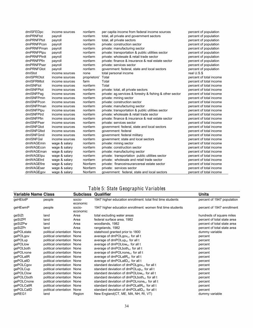
34

dmISFEDpc income sources nonfarm per capita income from federal income sources percent of population dmPRNFtot payroll nonfarm total, all private and government sectors percent of population dmPRNFPtot payroll nonfarm total, all private sectors percent of population dmPRNFPcon payroll nonfarm private: construction sector percent of population dmPRNFPman payroll nonfarm private: manufacturing sector percent of population dmPRNFPtpu payroll nonfarm private: transportation & public utilities sector percent of population dmPRNFPtrdt payroll nonfarm private: wholesale & retail trade sector percent of population dmPRNFPfin payroll nonfarm private: finance & insurance & real estate sector percent of population dmPRNFPser payroll nonfarm private: services sector percent of population dmPRNFGtot payroll nonfarm government: federal, state and local sectors percent of population dmIStot income sources none total personal income real U.S.$ dmISPROtot income sources proprietors' Total percent of total income dmISFRMtot income sources farm Total percent of total income dmISNFtot income sources nonfarm Total percent of total income dmISNFPtot income sources nonfarm private: total, all private sectors percent of total income dmISNFPag income sources nonfarm private: ag.services & forestry & fishing & other sector percent of total income dmISNFPmin income sources nonfarm private: mining sector percent of total income dmISNFPcon income sources nonfarm private: construction sector percent of total income dmISNFPman income sources nonfarm private: manufacturing sector percent of total income dmISNFPtpu income sources nonfarm private: transportation & public utilities sector percent of total income dmISNFPtrd income sources nonfarm private: wholesale & retail trade sector percent of total income dmISNFPfin income sources nonfarm private: finance & insurance & real estate sector percent of total income dmISNFPser income sources nonfarm private: services sector percent of total income dmISNFGtot income sources nonfarm government: federal, state and local sectors percent of total income dmISNFGfed income sources nonfarm government: federal percent of total income dmISNFGmil income sources nonfarm government: federal military percent of total income dmISNFGsl income sources nonfarm government: state and local sectors percent of total income dmWAGEmin wage & salary nonfarm private: mining sector percent of total income dmWAGEcon wage & salary nonfarm private: construction sector percent of total income dmWAGEman wage & salary nonfarm private: manufacturing sector percent of total income dmWAGEtpu wage & salary nonfarm private: transportation public utilities sector percent of total income dmWAGEtrd wage & salary nonfarm private: wholesale and retail trade sector percent of total income dmWAGEfire wage & salary Nonfarm private: financeinsurancereal estate sector percent of total income dmWAGEser wage & salary Nonfarm private: services sector percent of total income dmWAGEgov wage & salary Nonfarm government: federal, state and local sectors percent of total income

Table 5: State G eographic Variables Variable Name Class Subclass Qualifier Units geHEtotP people socio-

economic 1947 higher education enrollment: total first time students percent of 1947 population

geHEwmP people socio-economic

1947 higher education enrollment: women first time students percent of 1947 enrollment

geSIZt land Area total excluding water areas hundreds of square miles geSIZPf land Area federal surface area, 1982 percent of total state area geSIZPw land Area woodlands, 1982 percent of total state area geSIZPr land Area rangelands, 1982 percent of total state area gePOLstate political orientation None statehood granted prior to 1800 dummy variable gePOLgov political orientation None average of dmPOLgovs,t for all t percent gePOLup political orientation None average of dmPOLups,t for all t percent gePOLlow political orientation None average of dmPOLlows,t for all t percent gePOLboth political orientation None average of dmPOLboths,t for all t percent gePOLnone political orientation None average of dmPOLnones,t for all t percent gePOLallR political orientation None average of dmPOLallRs,t for all t percent gePOLallD political orientation None average of dmPOLallDs,t for all t percent gePOLCgov political orientation None standard deviation of dmPOLgovs,t for all t percent gePOLCup political orientation None standard deviation of dmPOLups,t for all t percent gePOLClow political orientation None standard deviation of dmPOLlows,t for all t percent gePOLCboth political orientation None standard deviation of dmPOLboths,t for all t percent gePOLCnone political orientation None standard deviation of dmPOLnones,t for all t percent gePOLCallR political orientation None standard deviation of dmPOLallRs,t for all t percent gePOLCallD political orientation None standard deviation of dmPOLallDs,t for all t percent geREG1 land Region New England(CT, ME, MA, NH, RI, VT) dummy variable

35

geREG2 Land Region middle Atlantic (DE, MD, NJ, NY, PA) dummy variable geREG3 Land Region east north central (IL, IN, MI, OH, WI) dummy variable geREG4 Land Region west north central (IA, KS, MN, MO, NE, ND, SD) dummy variable geREG5 Land Region south Atlantic (AL, AR, FL, GA, KY, LA, MS, NC, SC, TN, VA, WV) dummy variable geREG6 Land Region east south central (AZ, NM, OK, TX) dummy variable geREG7 Land Region mountain (CO, ID, MT, UT, WY) dummy variable geREG8 Land Region Pacific (CA, NV, OR, WA) dummy variable geREG9 Land Region noncontiguous U.S. (AK, HI) dummy variable geREGatl Land Region east coast dummy variable geREGpac Land Region west coast dummy variable geREGcan Land Region Canada border dummy variable geREGmex Land Region Mexico border dummy variable geREGcon Land Region constant dummy variable geCRrt Land Climate rainy-tropical dummy variable geCRhst Land Climate humid-subtropical dummy variable geCRhc Land Climate humid-continental dummy variable geCRmt Land Climate marine-temperate dummy variable geCRmed Land Climate Mediterranean dummy variable geCRsa Land Climate semi-arid dummy variable geCRd Land Climate desert dummy variable geCRarc Land Climate arctic and sub-arctic dummy variable geCRalp Land Climate alpine dummy variable geMNau Land Resources gold deposits dummy variable geMNcoal Land Resources coal deposits dummy variable geMNfe Land Resources iron ore deposits dummy variable geMNgas Land Resources natural gas deposits dummy variable geMNmo Land Resources molybdenum deposits dummy variable geMNoil Land Resources petroleum deposits dummy variable geMNu Land Resources uranium deposits dummy variable geMNfuel Land Resources coal, natural gas and/or petroleum deposits dummy variable geMN Land Resources gold, coal, iron ore, natural gas, molybdenum, or petroleum deposits dummy variable geAGwt Land agricultural wheat production dummy variable geAGcn Land agricultural corn production dummy variable geAG Land agricultural wheat and/or corn production dummy variable

Table 6: Variables Associated with the U .S. as a Whole Variable Name Class Subclass Qualifier Units usFUELpp miscellaneous None average producer price for fuels real u.s.$ usDEFcw miscellaneous None chained weight deflator (1996=1.0) percent usDEFfw miscellaneous None fixed weight deflator (1996=1.0) percent usPOP miscellaneous None total population of 48 contiguous states (excluding DC) thousands of persons usINCtot miscellaneous None total income of 48 contiguous states (excluding DC) thousands of persons usGRW miscellaneous None U.S. growth rate percent usINF miscellaneous None U.S. inflation rate percent

36

F igure 1: Difference between Individual State and U .S. Average G rowth Rates, 1947-1997

37

Appendix Tables

Table A1: Regression A (1959 – 1997)a

Variable Method Estimate Standard Deviation

t-value H0: θi = 0 H0: θi ≠ 0

One-Sided Marginal

Significance Level

usGRW odr 0.9302812 0.0289600 32.12 0.00% *** lls 0.8378600 0.0531617 15.76 0.00% *** usINF odr 0.0000929 0.0001454 0.64 26.14% lls 0.0001690 0.0001344 1.26 10.44% usFUELpp odr -0.0019124 0.0003440 -5.56 0.00% *** lls -0.0019699 0.0003242 -6.08 0.00% *** geREGcon odr 0.0160398 0.0020163 7.96 0.00% *** lls 0.0203461 0.0019015 10.70 0.00% *** gePOLstate odr 0.0036382 0.0006269 5.80 0.00% *** lls 0.0034087 0.0001286 26.51 0.00% *** y0 odr -0.0012481 0.0001683 -7.42 0.00% *** lls -0.0015189 0.0000344 -44.21 0.00% *** Rho odr 0.0099271 0.0015337 6.47 0.00% *** lls 0.0046268 0.0004614 10.03 0.00% ***

R2 odr 99.9 lls 96.7

ℓ(∙) odr -9781.8 lls -12325.3

σε odr 163.1 nls 1032.7 lls 0.05554

σεy odr 165.2

lls Na σε

yt0 odr 39.2 lls Na

σεγ odr 0.00914

lls Na

*** indicates H0 is rejected at α = 5% significance level. ** indicates H0 is rejected at α = 10% significance level. * indicates H0 is rejected at α = 20% significance level. a ℓ(∙) denotes the value of the likehood function. [σε , σεy , σεyt0 , σγ] denotes the standard deviations of the estimated residuals, the measurement error of income, the measurement error for initial income y0 , and the model, respectively; the standard deviation σε is a weighted average of the measurement error standard deviations and the model standard deviation.

38

Table A2: Regression B (per capita; 1959 – 1997)a



One-Sided Marginal

Significance Level

usGRW odr 0.9164151 0.0305155 30.03 0.00% *** lls 0.8094562 0.0486160 16.65 0.00% *** usINF odr -0.0005217 0.0001752 -2.98 0.15% *** lls 0.0000344 0.0001224 0.28 38.94% usFUELpp odr -0.0022860 0.0004129 -5.54 0.00% *** lls -0.0018108 0.0003250 -5.57 0.00% *** geREGcon odr 0.0159364 0.0028225 5.65 0.00% *** lls 0.0251525 0.0017342 14.50 0.00% *** gePOLstate odr 0.0026335 0.0007548 3.49 0.02% *** lls 0.0024147 0.0001521 15.88 0.00% *** y0 odr -0.0005696 0.0002808 -2.03 2.13% *** lls -0.0019923 0.0000757 -26.31 0.00% *** rho odr 0.0100623 0.0015213 6.61 0.00% *** lls 0.0049265 0.0004665 10.56 0.00% *** rvTXTOTAL odr 0.0031377 0.0027695 1.13 12.87% lls 0.0082254 0.0008457 9.73 0.00% *** rvTXINCcor odr 0.0089821 0.0097420 0.92 17.83% lls 0.0034075 0.0028961 1.18 11.98% rvTXINCind odr 0.0032783 0.0030738 1.07 14.32% lls -0.0022551 0.0008762 -2.57 0.51% *** rvTXSALgen odr 0.0028672 0.0032352 0.89 18.78% lls -0.0002181 0.0008425 -0.26 39.79% rvTXPROP odr 0.0060951 0.0024430 2.49 0.63% *** lls 0.0022668 0.0005968 3.80 0.01% *** rvTRFtot odr 0.0090632 0.0046069 1.97 2.47% *** lls -0.0018527 0.0017677 -1.05 14.74% rvTRFedu odr 0.1209462 0.0185788 6.51 0.00% *** lls 0.0326072 0.0062439 5.22 0.00% *** rvTRFhwy odr -0.0036942 0.0127112 -0.29 38.57% lls -0.0250445 0.0039599 -6.32 0.00% *** spEDUtot odr -0.0210545 0.0033184 -6.34 0.00% *** lls -0.0119434 0.0010889 -10.97 0.00% *** spHWYtot odr -0.0017725 0.0098695 -0.18 42.87% lls -0.0061415 0.0024377 -2.52 0.59% *** spWELtot odr -0.0095676 0.0046721 -2.05 2.04% *** lls -0.0080643 0.0017390 -4.64 0.00% *** spCAPhwy odr -0.0129220 0.0136243 -0.95 17.15% lls 0.0182959 0.0041463 4.41 0.00% ***

R2 odr 99.9 lls 97.5

ℓ(∙) odr -9737.6 lls -12026.7

σε odr 161.4 nls 872.9 lls 0.04801

σεy odr 163.4

lls Na σε

yt0 odr 40.7 lls Na

σεγ odr 0.00881

lls Na


39

Table A3: Regression C (per capita; 1959 – 1997)a



One-Sided Marginal

Significance Level

usGRW odr 0.9103451 0.0315407 28.86 0.00% *** lls 0.9114855 0.0458009 19.90 0.00% *** usINF odr -0.0008893 0.0002041 -4.36 0.00% *** lls -0.0001180 0.0001151 -1.03 15.26% usFUELpp odr -0.0034089 0.0005795 -5.88 0.00% *** lls -0.0034584 0.0004359 -7.93 0.00% *** geREGcon odr 0.0308275 0.0106647 2.89 0.19% *** lls 0.0359358 0.0031414 11.44 0.00% *** gePOLstate odr 0.0031325 0.0011917 2.63 0.43% *** lls 0.0018480 0.0002333 7.92 0.00% *** y0 odr 0.0016896 0.0005873 2.88 0.20% *** lls -0.0008591 0.0001285 -6.68 0.00% *** Rho odr 0.0099415 0.0015490 6.42 0.00% *** lls 0.0080705 0.0005671 14.23 0.00% *** rvTXTOTAL odr -0.0025031 0.0037391 -0.67 25.17% lls 0.0024610 0.0016153 1.52 6.39% * rvTXINCcor odr 0.0178962 0.0121115 1.48 6.98% * lls 0.0093894 0.0043028 2.18 1.46% *** rvTXINCind odr 0.0127397 0.0039577 3.22 0.07% *** lls -0.0007078 0.0014570 -0.49 31.36% rvTXSALgen odr 0.0100464 0.0041880 2.40 0.83% *** lls 0.0004336 0.0012976 0.33 36.91% rvTXPROP odr 0.0127685 0.0043262 2.95 0.16% *** lls 0.0097438 0.0014494 6.72 0.00% *** rvTRFtot odr 0.0194855 0.0057389 3.40 0.04% *** lls -0.0077557 0.0025860 -3.00 0.14% *** rvTRFedu odr 0.1577795 0.0217607 7.25 0.00% *** lls 0.0443102 0.0087588 5.06 0.00% *** rvTRFhwy odr 0.0039490 0.0153767 0.26 39.87% lls 0.0234687 0.0062073 3.78 0.01% *** spEDUtot odr -0.0287435 0.0044638 -6.44 0.00% *** lls -0.0081807 0.0020084 -4.07 0.00% *** spHWYtot odr -0.0426024 0.0155098 -2.75 0.30% *** lls -0.0108664 0.0047621 -2.28 1.13% *** spWELtot odr -0.0193764 0.0059203 -3.27 0.05% *** lls -0.0039471 0.0029446 -1.34 9.01% * spCAPhwy odr 0.0149744 0.0185924 0.81 21.03% lls -0.0022078 0.0064458 -0.34 36.60% dmPOLgov odr -0.0010380 0.0008451 -1.23 10.98% lls -0.0022265 0.0005086 -4.38 0.00% *** dmTXref odr -0.0017153 0.0011325 -1.51 6.50% * lls 0.0000856 0.0005383 0.16 43.68% dmTXsvl odr 0.0000085 0.0000774 0.11 45.61% lls 0.0000588 0.0000208 2.83 0.24% *** dmPOP odr -0.0001841 0.0001553 -1.19 11.80% lls -0.0000097 0.0000355 -0.27 39.20% dmDEN odr -0.0005325 0.0012430 -0.43 33.42% lls -0.0001418 0.0002607 -0.54 29.32% dmWAGEcv odr -0.0116700 0.0124409 -0.94 17.42% lls -0.0236378 0.0041351 -5.72 0.00% *** dmPRNFPcv odr 0.0064222 0.0102452 0.63 26.54% lls 0.0071484 0.0028476 2.51 0.61% *** geHEtotP odr -0.5747542 0.1350808 -4.25 0.00% *** lls -0.2797150 0.0302948 -9.23 0.00% *** geSIZ odr 0.0000497 0.0000235 2.12 1.73% *** lls 0.0000221 0.0000039 5.61 0.00% *** geSIZPf odr -0.0000703 0.0000352 -1.99 2.31% *** lls -0.0000433 0.0000083 -5.22 0.00% *** geREGatl odr 0.0005882 0.0013128 0.45 32.71% lls 0.0000483 0.0002643 0.18 42.74%

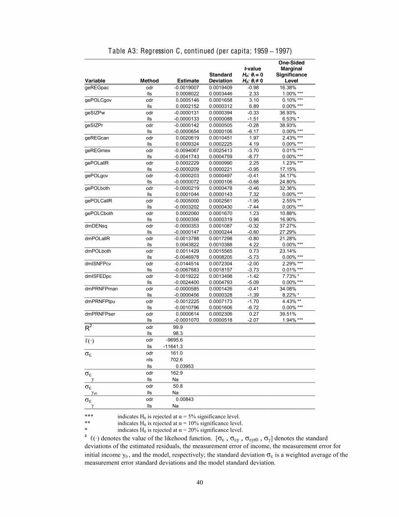
40

Table A3: Regression C , continued (per capita; 1959 – 1997)



One-Sided Marginal

Significance Level

geREGpac odr -0.0019007 0.0019409 -0.98 16.38% lls 0.0008022 0.0003446 2.33 1.00% *** gePOLCgov odr 0.0005146 0.0001658 3.10 0.10% *** lls 0.0002152 0.0000312 6.89 0.00% *** geSIZPw odr -0.0000131 0.0000394 -0.33 36.93% lls -0.0000133 0.0000088 -1.51 6.53% * geSIZPr odr -0.0000142 0.0000505 -0.28 38.93% lls -0.0000654 0.0000106 -6.17 0.00% *** geREGcan odr 0.0020619 0.0010451 1.97 2.43% *** lls 0.0009324 0.0002225 4.19 0.00% *** geREGmex odr -0.0094067 0.0025413 -3.70 0.01% *** lls -0.0041743 0.0004759 -8.77 0.00% *** gePOLallR odr 0.0002229 0.0000990 2.25 1.23% *** lls -0.0000209 0.0000221 -0.95 17.15% gePOLgov odr -0.0000203 0.0000497 -0.41 34.17% lls -0.0000072 0.0000106 -0.68 24.80% gePOLboth odr -0.0000219 0.0000478 -0.46 32.36% lls 0.0001044 0.0000143 7.32 0.00% *** gePOLCallR odr -0.0005000 0.0002561 -1.95 2.55% ** lls -0.0003202 0.0000430 -7.44 0.00% *** gePOLCboth odr 0.0002060 0.0001670 1.23 10.88% lls 0.0000306 0.0000319 0.96 16.90% dmDENsq odr -0.0000353 0.0001087 -0.32 37.27% lls -0.0000147 0.0000244 -0.60 27.29% dmPOLallR odr -0.0013788 0.0017298 -0.80 21.28% lls 0.0043822 0.0010388 4.22 0.00% *** dmPOLboth odr 0.0011429 0.0015565 0.73 23.14% lls -0.0046978 0.0008205 -5.73 0.00% *** dmISNFPcv odr -0.0144514 0.0072304 -2.00 2.29% *** lls -0.0067683 0.0018157 -3.73 0.01% *** dmISFEDpc odr -0.0019222 0.0013498 -1.42 7.73% * lls -0.0024400 0.0004793 -5.09 0.00% *** dmPRNFPman odr -0.0000585 0.0001426 -0.41 34.08% lls -0.0000456 0.0000328 -1.39 8.22% * dmPRNFPtpu odr -0.0012225 0.0007173 -1.70 4.43% ** lls -0.0010796 0.0001606 -6.72 0.00% *** dmPRNFPser odr 0.0000614 0.0002306 0.27 39.51% lls -0.0001070 0.0000518 -2.07 1.94% ***

R2 odr 99.9 lls 98.3

ℓ(∙) odr -9695.6 lls -11641.3

σε odr 161.0 nls 702.6 lls 0.03953

σεy odr 162.9

lls Na σε

yt0 odr 50.8 lls Na

σεγ odr 0.00843

lls Na


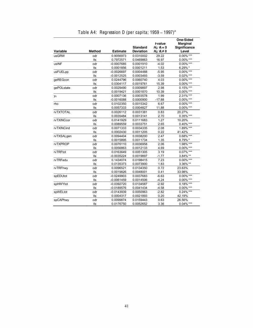
41

Table A4: Regression D (per capita; 1959 – 1997)a



One-Sided Marginal

Significance Level

usGRW odr 0.9056973 0.0310002 29.22 0.00% *** lls 0.7972571 0.0469863 16.97 0.00% *** usINF odr -0.0007685 0.0001910 -4.02 0.00% *** lls 0.0001856 0.0001211 1.53 6.29% * usFUELpp odr -0.0026697 0.0004488 -5.95 0.00% *** lls -0.0012525 0.0003493 -3.59 0.02% *** geREGcon odr 0.0244796 0.0060740 4.03 0.00% *** lls 0.0304117 0.0019761 15.39 0.00% *** gePOLstate odr 0.0029490 0.0009897 2.98 0.15% *** lls 0.0019421 0.0001870 10.39 0.00% *** y0 odr 0.0007136 0.0003578 1.99 2.31% *** lls -0.0016088 0.0000900 -17.88 0.00% *** rho odr 0.0102350 0.0015342 6.67 0.00% *** lls 0.0057333 0.0004827 11.88 0.00% *** rvTXTOTAL odr 0.0026112 0.0031381 0.83 20.27% lls 0.0035484 0.0013141 2.70 0.35% *** rvTXINCcor odr 0.0141929 0.0111683 1.27 10.20% lls 0.0089559 0.0033751 2.65 0.40% *** rvTXINCind odr 0.0071333 0.0034335 2.08 1.89% *** lls 0.0002430 0.0011205 0.22 41.42% rvTXSALgen odr 0.0094404 0.0038200 2.47 0.68% *** lls 0.0015895 0.0011734 1.35 8.79% * rvTXPROP odr 0.0076110 0.0036958 2.06 1.98% *** lls 0.0056863 0.0012133 4.69 0.00% *** rvTRFtot odr 0.0163649 0.0051305 3.19 0.07% *** lls -0.0035224 0.0019897 -1.77 3.84% ** rvTRFedu odr 0.1434074 0.0198415 7.23 0.00% *** lls 0.0135373 0.0073900 1.83 3.36% ** rvTRFhwy odr 0.0096521 0.0134350 0.72 23.63% lls 0.0019826 0.0048001 0.41 33.98% spEDUtot odr -0.0249903 0.0037683 -6.63 0.00% *** lls -0.0061459 0.0014506 -4.24 0.00% *** spHWYtot odr -0.0392720 0.0134587 -2.92 0.18% *** lls -0.0189576 0.0041434 -4.58 0.00% *** spWELtot odr -0.0143939 0.0050963 -2.82 0.24% *** lls 0.0004317 0.0021893 0.20 42.19% spCAPhwy odr 0.0099874 0.0159443 0.63 26.56% lls 0.0176750 0.0052652 3.36 0.04% ***

42

Table A4: Regression D , continued (per capita; 1959 – 1997)



One-Sided Marginal

Significance Level

dmPOLgov odr -0.0010235 0.0007508 -1.36 8.65% * lls -0.0016824 0.0003849 -4.37 0.00% *** dmTXref odr -0.0015992 0.0010437 -1.53 6.28% * lls -0.0010759 0.0004708 -2.29 1.12% *** dmTXsvl odr -0.0001107 0.0000693 -1.60 5.53% * lls -0.0000242 0.0000197 -1.23 11.01% dmPOP odr -0.0002824 0.0001148 -2.46 0.70% *** lls -0.0001299 0.0000274 -4.75 0.00% *** dmDEN odr -0.0011047 0.0002829 -3.90 0.00% *** lls -0.0004231 0.0000603 -7.02 0.00% *** dmWAGEcv odr 0.0154413 0.0102397 1.51 6.59% * lls -0.0165814 0.0034684 -4.78 0.00% *** dmPRNFPcv odr -0.0071238 0.0032788 -2.17 1.50% *** lls -0.0015837 0.0007087 -2.23 1.28% *** geHEtotP odr -0.2951371 0.0972264 -3.04 0.12% *** lls -0.1513898 0.0210277 -7.20 0.00% *** geSIZ odr 0.0000054 0.0000115 0.47 31.86% lls -0.0000050 0.0000023 -2.15 1.57% *** geSIZPf odr -0.0000626 0.0000254 -2.46 0.70% *** lls -0.0000201 0.0000057 -3.54 0.02% *** geREGatl odr 0.0013876 0.0009819 1.41 7.89% * lls 0.0007583 0.0001852 4.09 0.00% *** geREGpac odr -0.0027652 0.0015502 -1.78 3.73% ** lls 0.0011817 0.0003036 3.89 0.01% *** gePOLCgov odr 0.0001881 0.0001157 1.62 5.22% * lls 0.0000565 0.0000213 2.65 0.41% ***

R2 odr 99.9 lls 97.9

ℓ(∙) odr -9712.0 lls -11845.7

σε odr 161.2 nls 788.3 lls 0.0

σεy odr 163.1

lls na σε

yt0 odr 49.5 lls na

σεγ odr 0.00857

lls na


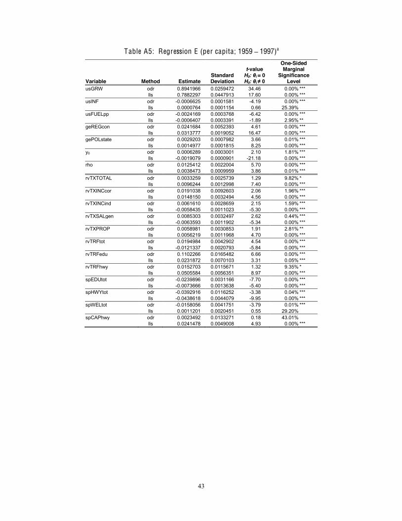
43

Table A5: Regression E (per capita; 1959 – 1997)a



One-Sided Marginal

Significance Level

usGRW odr 0.8941966 0.0259472 34.46 0.00% *** lls 0.7882297 0.0447913 17.60 0.00% *** usINF odr -0.0006625 0.0001581 -4.19 0.00% *** lls 0.0000764 0.0001154 0.66 25.39% usFUELpp odr -0.0024169 0.0003768 -6.42 0.00% *** lls -0.0006407 0.0003391 -1.89 2.95% ** geREGcon odr 0.0241684 0.0052393 4.61 0.00% *** lls 0.0313777 0.0019052 16.47 0.00% *** gePOLstate odr 0.0029203 0.0007982 3.66 0.01% *** lls 0.0014977 0.0001815 8.25 0.00% *** y0 odr 0.0006289 0.0003001 2.10 1.81% *** lls -0.0019079 0.0000901 -21.18 0.00% *** rho odr 0.0125412 0.0022004 5.70 0.00% *** lls 0.0038473 0.0009959 3.86 0.01% *** rvTXTOTAL odr 0.0033259 0.0025739 1.29 9.82% * lls 0.0096244 0.0012998 7.40 0.00% *** rvTXINCcor odr 0.0191038 0.0092603 2.06 1.96% *** lls 0.0148150 0.0032494 4.56 0.00% *** rvTXINCind odr 0.0061610 0.0028659 2.15 1.59% *** lls -0.0058435 0.0011023 -5.30 0.00% *** rvTXSALgen odr 0.0085303 0.0032497 2.62 0.44% *** lls -0.0063593 0.0011902 -5.34 0.00% *** rvTXPROP odr 0.0058981 0.0030853 1.91 2.81% ** lls 0.0056219 0.0011968 4.70 0.00% *** rvTRFtot odr 0.0194984 0.0042902 4.54 0.00% *** lls -0.0121337 0.0020793 -5.84 0.00% *** rvTRFedu odr 0.1102266 0.0165482 6.66 0.00% *** lls 0.0231872 0.0070103 3.31 0.05% *** rvTRFhwy odr 0.0152703 0.0115671 1.32 9.35% * lls 0.0505584 0.0056351 8.97 0.00% *** spEDUtot odr -0.0239896 0.0031166 -7.70 0.00% *** lls -0.0073666 0.0013638 -5.40 0.00% *** spHWYtot odr -0.0392916 0.0116252 -3.38 0.04% *** lls -0.0438618 0.0044079 -9.95 0.00% *** spWELtot odr -0.0158056 0.0041751 -3.79 0.01% *** lls 0.0011201 0.0020451 0.55 29.20% spCAPhwy odr 0.0023492 0.0133271 0.18 43.01% lls 0.0241478 0.0049008 4.93 0.00% ***

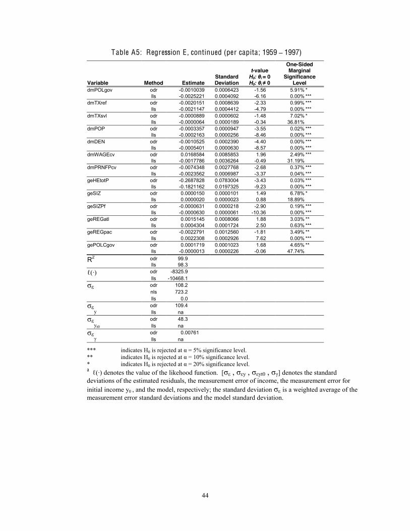
44

Table A5: Regression E , continued (per capita; 1959 – 1997)



One-Sided Marginal

Significance Level

dmPOLgov odr -0.0010039 0.0006423 -1.56 5.91% * lls -0.0025221 0.0004092 -6.16 0.00% *** dmTXref odr -0.0020151 0.0008639 -2.33 0.99% *** lls -0.0021147 0.0004412 -4.79 0.00% *** dmTXsvl odr -0.0000889 0.0000602 -1.48 7.02% * lls -0.0000064 0.0000189 -0.34 36.81% dmPOP odr -0.0003357 0.0000947 -3.55 0.02% *** lls -0.0002163 0.0000256 -8.46 0.00% *** dmDEN odr -0.0010525 0.0002390 -4.40 0.00% *** lls -0.0005401 0.0000630 -8.57 0.00% *** dmWAGEcv odr 0.0168584 0.0085853 1.96 2.49% *** lls -0.0017786 0.0036264 -0.49 31.19% dmPRNFPcv odr -0.0074348 0.0027768 -2.68 0.37% *** lls -0.0023562 0.0006987 -3.37 0.04% *** geHEtotP odr -0.2687828 0.0783004 -3.43 0.03% *** lls -0.1821162 0.0197325 -9.23 0.00% *** geSIZ odr 0.0000150 0.0000101 1.49 6.78% * lls 0.0000020 0.0000023 0.88 18.89% geSIZPf odr -0.0000631 0.0000218 -2.90 0.19% *** lls -0.0000630 0.0000061 -10.36 0.00% *** geREGatl odr 0.0015145 0.0008066 1.88 3.03% ** lls 0.0004304 0.0001724 2.50 0.63% *** geREGpac odr -0.0022791 0.0012560 -1.81 3.49% ** lls 0.0022308 0.0002926 7.62 0.00% *** gePOLCgov odr 0.0001719 0.0001023 1.68 4.65% ** lls -0.0000013 0.0000226 -0.06 47.74%

R2 odr 99.9 lls 98.3

ℓ(∙) odr -8325.9 lls -10468.1

σε odr 108.2 nls 723.2 lls 0.0

σεy odr 109.4

lls na σε

yt0 odr 48.3 lls na

σεγ odr 0.00761

lls na


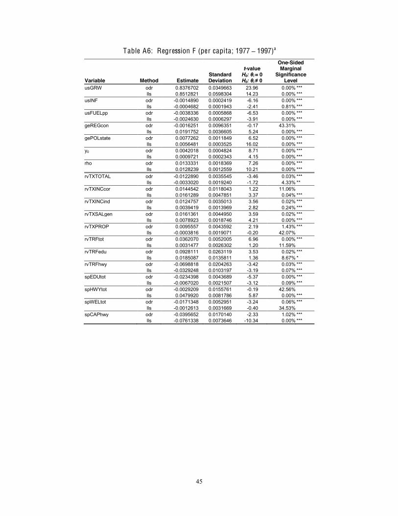
45

Table A6: Regression F (per capita; 1977 – 1997)a



One-Sided Marginal

Significance Level

usGRW odr 0.8376702 0.0349663 23.96 0.00% *** lls 0.8512821 0.0598304 14.23 0.00% *** usINF odr -0.0014890 0.0002419 -6.16 0.00% *** lls -0.0004682 0.0001943 -2.41 0.81% *** usFUELpp odr -0.0038336 0.0005868 -6.53 0.00% *** lls -0.0024630 0.0006297 -3.91 0.00% *** geREGcon odr -0.0016251 0.0096351 -0.17 43.31% lls 0.0191752 0.0036605 5.24 0.00% *** gePOLstate odr 0.0077262 0.0011849 6.52 0.00% *** lls 0.0056481 0.0003525 16.02 0.00% *** y0 odr 0.0042018 0.0004824 8.71 0.00% *** lls 0.0009721 0.0002343 4.15 0.00% *** rho odr 0.0133331 0.0018369 7.26 0.00% *** lls 0.0128239 0.0012559 10.21 0.00% *** rvTXTOTAL odr -0.0122890 0.0035545 -3.46 0.03% *** lls -0.0033020 0.0019240 -1.72 4.33% ** rvTXINCcor odr 0.0144542 0.0118043 1.22 11.06% lls 0.0161289 0.0047851 3.37 0.04% *** rvTXINCind odr 0.0124757 0.0035013 3.56 0.02% *** lls 0.0039419 0.0013969 2.82 0.24% *** rvTXSALgen odr 0.0161361 0.0044950 3.59 0.02% *** lls 0.0078923 0.0018746 4.21 0.00% *** rvTXPROP odr 0.0095557 0.0043592 2.19 1.43% *** lls -0.0003816 0.0019071 -0.20 42.07% rvTRFtot odr 0.0362070 0.0052005 6.96 0.00% *** lls 0.0031477 0.0026302 1.20 11.59% rvTRFedu odr 0.0928111 0.0263119 3.53 0.02% *** lls 0.0185087 0.0135811 1.36 8.67% * rvTRFhwy odr -0.0698818 0.0204263 -3.42 0.03% *** lls -0.0329248 0.0103197 -3.19 0.07% *** spEDUtot odr -0.0234398 0.0043689 -5.37 0.00% *** lls -0.0067020 0.0021507 -3.12 0.09% *** spHWYtot odr -0.0029209 0.0155761 -0.19 42.56% lls 0.0479920 0.0081786 5.87 0.00% *** spWELtot odr -0.0171348 0.0052951 -3.24 0.06% *** lls -0.0012613 0.0031669 -0.40 34.53% spCAPhwy odr -0.0395652 0.0170140 -2.33 1.02% *** lls -0.0761338 0.0073646 -10.34 0.00% ***

46

Table A6: Regression F , continued (per capita; 1977 – 1997)



One-Sided Marginal

Significance Level

dmPOLgov odr -0.0017111 0.0008823 -1.94 2.64% ** lls -0.0007516 0.0005810 -1.29 9.81% * dmTXref odr -0.0028185 0.0010270 -2.74 0.31% *** lls -0.0009378 0.0004808 -1.95 2.57% ** dmTXsvl odr 0.0000372 0.0001121 0.33 37.00% lls -0.0000658 0.0000448 -1.47 7.09% * dmPOP odr -0.0005841 0.0001388 -4.21 0.00% *** lls -0.0003146 0.0000591 -5.33 0.00% *** dmDEN odr -0.0010891 0.0003317 -3.28 0.05% *** lls 0.0001125 0.0001294 0.87 19.24% dmWAGEcv odr -0.0031714 0.0143935 -0.22 41.28% lls -0.0152187 0.0073483 -2.07 1.93% *** dmPRNFPcv odr -0.0278520 0.0062530 -4.45 0.00% *** lls -0.0140347 0.0025069 -5.60 0.00% *** geHEtotP odr -0.0160173 0.1250571 -0.13 44.91% lls 0.0092005 0.0421378 0.22 41.36% geSIZ odr 0.0000145 0.0000166 0.87 19.11% lls 0.0000114 0.0000058 1.96 2.55% ** geSIZPf odr 0.0000267 0.0000324 0.83 20.47% lls 0.0000049 0.0000123 0.40 34.57% geREGatl odr 0.0041014 0.0011744 3.49 0.03% *** lls 0.0042574 0.0004006 10.63 0.00% *** geREGpac odr -0.0081298 0.0020384 -3.99 0.00% *** lls -0.0020239 0.0007513 -2.69 0.36% *** gePOLCgov odr 0.0004209 0.0001793 2.35 0.96% *** lls -0.0000669 0.0000583 -1.15 12.60%

R2 odr 99.9 lls 97.3

ℓ(∙) odr -4257.8 lls -5270.8

σε odr 103.6 nls 638.6 lls 0.0

σεy odr 105.9

lls na σε

yt0 odr 42.8 lls na

σεγ odr 0.00751

lls na


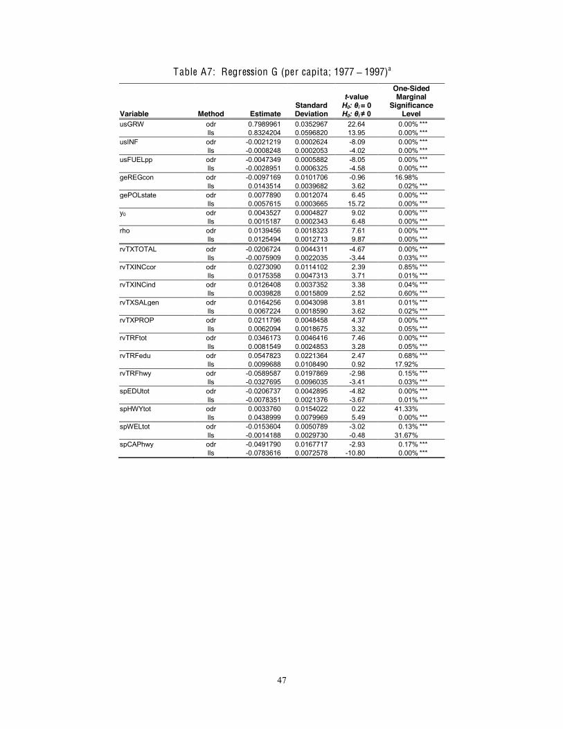
47

Table A7: Regression G (per capita; 1977 – 1997)a



One-Sided Marginal

Significance Level

usGRW odr 0.7989961 0.0352967 22.64 0.00% *** lls 0.8324204 0.0596820 13.95 0.00% *** usINF odr -0.0021219 0.0002624 -8.09 0.00% *** lls -0.0008248 0.0002053 -4.02 0.00% *** usFUELpp odr -0.0047349 0.0005882 -8.05 0.00% *** lls -0.0028951 0.0006325 -4.58 0.00% *** geREGcon odr -0.0097169 0.0101706 -0.96 16.98% lls 0.0143514 0.0039682 3.62 0.02% *** gePOLstate odr 0.0077890 0.0012074 6.45 0.00% *** lls 0.0057615 0.0003665 15.72 0.00% *** y0 odr 0.0043527 0.0004827 9.02 0.00% *** lls 0.0015187 0.0002343 6.48 0.00% *** rho odr 0.0139456 0.0018323 7.61 0.00% *** lls 0.0125494 0.0012713 9.87 0.00% *** rvTXTOTAL odr -0.0206724 0.0044311 -4.67 0.00% *** lls -0.0075909 0.0022035 -3.44 0.03% *** rvTXINCcor odr 0.0273090 0.0114102 2.39 0.85% *** lls 0.0175358 0.0047313 3.71 0.01% *** rvTXINCind odr 0.0126408 0.0037352 3.38 0.04% *** lls 0.0039828 0.0015809 2.52 0.60% *** rvTXSALgen odr 0.0164256 0.0043098 3.81 0.01% *** lls 0.0067224 0.0018590 3.62 0.02% *** rvTXPROP odr 0.0211796 0.0048458 4.37 0.00% *** lls 0.0062094 0.0018675 3.32 0.05% *** rvTRFtot odr 0.0346173 0.0046416 7.46 0.00% *** lls 0.0081549 0.0024853 3.28 0.05% *** rvTRFedu odr 0.0547823 0.0221364 2.47 0.68% *** lls 0.0099688 0.0108490 0.92 17.92% rvTRFhwy odr -0.0589587 0.0197869 -2.98 0.15% *** lls -0.0327695 0.0096035 -3.41 0.03% *** spEDUtot odr -0.0206737 0.0042895 -4.82 0.00% *** lls -0.0078351 0.0021376 -3.67 0.01% *** spHWYtot odr 0.0033760 0.0154022 0.22 41.33% lls 0.0438999 0.0079969 5.49 0.00% *** spWELtot odr -0.0153604 0.0050789 -3.02 0.13% *** lls -0.0014188 0.0029730 -0.48 31.67% spCAPhwy odr -0.0491790 0.0167717 -2.93 0.17% *** lls -0.0783616 0.0072578 -10.80 0.00% ***

48

Table A7: Regression G , continued (per capita; 1977 – 1997)



One-Sided Marginal

Significance Level

dmPOLgov odr -0.0014138 0.0008758 -1.61 5.34% * lls -0.0004223 0.0005660 -0.75 22.79% dmTXref odr -0.0030315 0.0010073 -3.01 0.13% *** lls -0.0013786 0.0004681 -2.95 0.17% *** dmTXsvl odr 0.0002713 0.0000952 2.85 0.22% *** lls 0.0000731 0.0000348 2.10 1.79% *** dmPOP odr -0.0006322 0.0001390 -4.55 0.00% *** lls -0.0003765 0.0000566 -6.65 0.00% *** dmDEN odr -0.0011308 0.0003329 -3.40 0.04% *** lls -0.0000422 0.0001288 -0.33 37.17% dmWAGEcv odr -0.0127627 0.0144083 -0.89 18.80% lls -0.0256473 0.0070387 -3.64 0.01% *** dmPRNFPcv odr -0.0265801 0.0062039 -4.28 0.00% *** lls -0.0170890 0.0025164 -6.79 0.00% *** geHEtotP odr -0.0110668 0.1237472 -0.09 46.44% lls -0.0019649 0.0416799 -0.05 48.12% geSIZ odr 0.0000182 0.0000167 1.09 13.79% lls 0.0000138 0.0000058 2.37 0.90% *** geSIZPf odr 0.0000338 0.0000324 1.04 14.89% lls 0.0000172 0.0000124 1.38 8.42% * geREGatl odr 0.0044051 0.0011685 3.77 0.01% *** lls 0.0041443 0.0003931 10.54 0.00% *** geREGpac odr -0.0089170 0.0020430 -4.36 0.00% *** lls -0.0032424 0.0007670 -4.23 0.00% *** gePOLCgov odr 0.0004479 0.0001823 2.46 0.71% *** lls -0.0000060 0.0000606 -0.10 46.09%

R2 odr 99.9 lls 97.3

ℓ(∙) odr -4255.6 lls -5265.6

σε odr 104.4 nls 634.6 lls 0.0

σεy odr 106.7

lls na σε

yt0 odr 43.3 lls na

σεγ odr 0.00745

lls Na


Documents

Do State Fiscal Policies Affect State Economic Growth?