Do Strategic Substitutes Make Better Markets? A Comparison of Bertrand and Cournot Markets

Douglas Davis*

20 January 2009

Abstract

Recent experiments suggest that games where actions are strategic substitutes rather than strategic complements exhibit some desirable performance characteristics. This paper reports an experiment conducted to test whether these characteristics extend to differentiated product Cournot and Bertrand markets. We find that Cournot markets do not generally outperform Bertrand markets, and that the opposite is often true. Bertrand markets exhibit comparatively higher convergence levels and speeds, particularly when products are close substitutes. Bertrand sellers do engage in more signaling activity than Cournot sellers. Such efforts, however, affect market outcomes only occasionally, and only when products are differentiated. Analysis of individual decisions suggests that the observed differences in convergence levels and speeds are driven by a propensity for sellers to use forecast and inertia anchors as bases for action choices in addition to best replies. Given these propensities, Bertrand markets converge more rapidly and more completely to static Nash predictions, particularly when products are close substitutes, because the differences between the various anchors is smaller in Bertrand markets.

Keywords: Experiments, Market Concentration, Market Power

JEL codes C9, D4 and L4

_____________________________________ * Virginia Commonwealth University, Richmond VA 23284-4000, (804) 828-7140. e-mail: dddavis@vcu.edu. Thanks to Asen Ivanov, Lise Vesterlund, Oleg Korenok, Robert Reilly and Roger Sherman for their useful comments. The usual disclaimer applies. Thanks also to Matthew Nuckols for programming assistance. Financial assistance from the National Science Foundation (SES 0518829) and the Virginia Commonwealth University Summer Research Grants Program is gratefully acknowledged.

I. Introduction

A series of important recent experiments suggest that alterations in the strategic relationship of actions in a game can importantly affect behavioral outcomes. At issue is whether actions are strategic complements or strategic substitutes. Given an ordering of actions, actions are strategic complements when higher action choices by one player provide an incentive for others to make higher action choices as well. Actions are strategic substitutes when the reverse is true, that is, when higher action choices by one player provides an incentive for others to reduce their action choices. Perhaps the readiest illustration of such an alteration in strategic relationships is the comparison of Bertrand and Cournot oligopolies. In a standard Bertrand environment, price choices are strategic complements. A seller’s best response to, say, a positive price deviation by other sellers is to post a similar, albeit slightly lower own price. In a Cournot environment, quantity decisions are strategic substitutes. A seller’s best response to a positive quantity deviation by other sellers is to reduce his or her own quantity.

Experiments conducted in carefully stylized environments show that when all else is held fixed, a context where actions are strategic substitutes tends to (a) converge more completely to static Nash equilibrium predictions, (b) adjust more quickly to anticipated nominal shocks and (c) be less prone to tacit collusion, than a comparable context where actions are strategic complements. These behavioral results have potentially important implications for industrial organization. Among other things, they suggest that an analyst’s decision to characterize a specific context as involving Cournot rather than Bertrand interactions carries with it implications regarding stability, responsiveness and susceptibility to tacit collusion. These results also suggest that those institutions where actions are strategic substitutes may, as a matter of institutional design, be preferred.1

Such implications come as something of a surprise to those familiar with the behavioral oligopoly literature. Several investigators have noted the slow and incomplete convergence in laboratory Cournot markets (e.g., Rassenti, Reynolds, Smith and Szidarosky, 2000, Offerman, Potters, Sonnemans, 2002), with the differences being particularly pronounced when compared to Bertrand markets (Davis, 1999, 2002).2

1 In addition to the standard comparisons of equilibrium pricing and output decisions among firms, Bertrand/Cournot games have been comparatively analyzed in a variety of other contexts, including, managerial compensation, information pooling arrangements, strategic alliances and research and development expenditures. (Daughety, 2008 concisely reviews the recent literature.) These diverse applications suggest that the choice of strategy interactions may reasonably be considered as a question of institutional design. 2 However, Huck, Norman and Oechssler (2002) ‘HNO’ do cleanly show that laboratory Cournot markets do not exhibit the explosive instability predicted by Theocharis (1960). (Theocharis observes that a Cournot game with linear demand and constant unit costs is explosively unstable to a Cournot (purely adaptive) best response dynamic. Fisher (1961) and others showed that increasing marginal costs or some inertia in the adjustment process can restore stability.) HNO report a Cournot experiment in a quadropoly design, where variations in the probability that sellers could adjust quantities each period created Cournot games that were variously stable and unstable to a Cournot best response dynamic. HNO find that their markets were uniformly stable, and that variations in the probability of adjustment did not affect performance. They attribute their results to a tendency for many sellers follow a strategy of imitating the average choice of other sellers rather than a Cournot best response dynamic.

In terms of the more recent theoretical literature on lattice structures (Topkis, 1979), games where actions are strategic complements, such as the Bertrand games we study here, are supermodular, while games where actions are strategic substitutes, such as Cournot games with

Further, although a recent meta-analysis of oligopoly experiments by Suetens and Potters (2007) concludes that Bertrand markets are more susceptible to tacit collusion than Cournot markets, the conclusion is based mostly on comparisons of Cournot and Bertrand duopolies. Evidence regarding behavior in thicker markets, particularly those with more than three sellers is considerably less convincing.3

This paper reports an experiment conducted to examine this apparent inconsistency in the behavioral literature. Here, we examine the performance of differentiated product quadropolies with a common linear demand structure, and constant unit costs. Treatments are combinations of the institution (Cournot or Bertrand) and the degree of product substitutability (low or high). By way of pre-summary, we find that Cournot markets do not generally outperform Bertrand markets, and that the opposite is often true. Bertrand markets exhibit comparatively higher convergence levels and speeds, particularly when products are close substitutes. Further, although the incidence of signaling activity is higher in Bertrand markets than in Cournot markets, such efforts result in increased prices only occasionally, and only when products are differentiated. We conjecture that a type of bounded rationality explains the relatively low convergence levels and speeds in our Cournot markets. However, instead of differences in sellers’ capacities to adopt forward-looking expectations (as is the focus in strategic substitutes/ strategic complements literature), in our relatively complex market contexts we find that sellers vary with respect to the rationality of their action choices. In addition to making best replies, sellers often anchor their action choices on rules of thumb, such as their forecast of rivals’ next period actions or their own previous period action. In Cournot markets, the distance between best replies and these other anchors is much larger than in comparable Bertrand markets, and for this reason Cournot markets exhibit lower convergence speeds and levels. In turn, the increased outcome variability in Cournot markets undermines seller efforts to coordinate actions via signaling.

The remainder of this paper is organized as follows. Section 2 reviews the pertinent literature. Section 3 examines the relationship between Cournot and Bertrand games. Section 4 presents the experiment design and procedures. Results are presented in section 5, followed by some discussion of bounded rationality and market convergence in a sixth section. A short seventh section concludes.

more than two players are submodular. Supermodular games are robustly stable, with actions converging to the set of equilibrium outcomes under a wide variety of learning dynamics, including best response, adaptive play, fictitious play and Bayesian learning (Milgrom and Roberts, 1990). Submodular games do not satisfy the ‘contraction condition’ sufficient to generate the robust converge properties of their supermodular counterparts unless the slope of the best reply to the average of others actions is less than unitary (e.g., Vives, 1999 p. 150). The finding by HNO that parameter variations in the neighborhood of the contraction condition in a submodular game does not behaviorally affect stability parallels a finding in a game with strategic complements studied by Chen and Gazzale (2004) ,who similarly find that parameter alterations in the neighborhood of the supermodularity condition do not affect behavioral stability. 3 Davis (2002) and Huck, Normann and Oechssler (2000) examine behaviorally Bertrand and Cournot quadropolies. Neither study reports evidence of an increased tendency for tacit collusion in Bertrand markets, unless the set of feedback information for sellers includes other sellers’ earnings. Given such ‘extra’ information, imitation strategies tend to drive Cournot prices to the Walrasian predictions, as suggested by Vega Redondo (1997), making Bertrand markets relatively more collusive in the limited sense that Cournot markets yield infra-competitive outcomes.

2

2. Literature Review We focus on three recent experimental papers that examine strategic substitutes and strategic complements. A first paper, Heemeijer, Hommes, Sonnemans and Tuinstra (2007,‘HHST’), examines a series of six-seller ‘prediction’ markets, where sellers earn profits by forecasting the next period price more accurately than their rivals. The experiment consists of two treatments, which differ only in the strategic relation between seller forecasts and the induced market price response.4 In a ‘positive feedback’ treatment, prices move directly with forecasts, making forecasts strategic complements. In the negative feedback treatment the reverse is true, making forecasts strategic substitutes. The authors report significantly higher convergence levels and speeds in the ‘negative feedback’ treatment.

HHST explain their results as a consequence of bounded rationality. Theoretical work by Haltiwanger and Waldman (1985) shows that for a given share of boundedly rational agents, the extent to which actions are strategic substitutes affects the speed of adjustment towards equilibrium. Intuitively, in contexts where actions are strategic substitutes, rational players have an incentive to move away from boundedly rational (adaptive) players, thus driving outcomes toward the equilibrium. In contrast, when actions are strategic complements, rational players optimize by moving toward actions of the boundedly rational players, slowing convergence

A second pertinent paper, Fehr and Tyran (2008), investigates the effects of alterations in the strategic relationship of actions on market responses to a fully announced nominal shock. These authors test the relative effects of strategic complements and strategic substitutes in a stylized four seller discrete choice price-setting game where the static Nash equilibrium is Pareto optimal. The game is presented to participants in a bi-matrix format that shows sellers the own profit consequences of their own and others’ average price choices. Each session consisted of two fifteen period sequences. At the conclusion of the first sequence, the investigators induce a shock that reduces the equilibrium price by half. At the same time, to keep the shock purely nominal, the investigators double the lab/currency exchange rate. To ensure that participants understood the consequences of the shock, they were given a new set of tables, and an opportunity to study them.

Fehr and Tyran report dramatic treatment effects in response to the shock. In the strategic substitutes treatment, adjustment to the new equilibrium was, for a large majority of participants (67%), immediate. In contrast, in the strategic complements treatment less than a quarter of participants (23%) adjusted immediately to the shock, and sellers needed ten periods to match the first period equilibrium play rate observed in the strategic substitute treatment. In part, Fehr and Tyran attribute their results to the same bounded rationality arguments discussed above as support for the results in HHST. However, analyzing individual forecasts and prices, Fehr and Tyran further argue that the nature of strategic interactions itself affects rationality, because strategic complementarity tends to make subject expectations less forward looking (and thus less rational).

Fehr and Tyran frame their argument in terms of seller responses to an announced nominal shock. In a game where actions are strategic complements, such as 4 HHST set parameters so that both the Nash equilibrium price and the absolute magnitude of the induced market response to forecasts are the same across treatments. Across treatments only the sign of the induced market response changes from positive to negative. Notice also that tacit collusion is not a consideration in this experiment. Sellers have no incentive to attempt to cooperate, because their earnings arise only from out-forecasting their rivals.

3

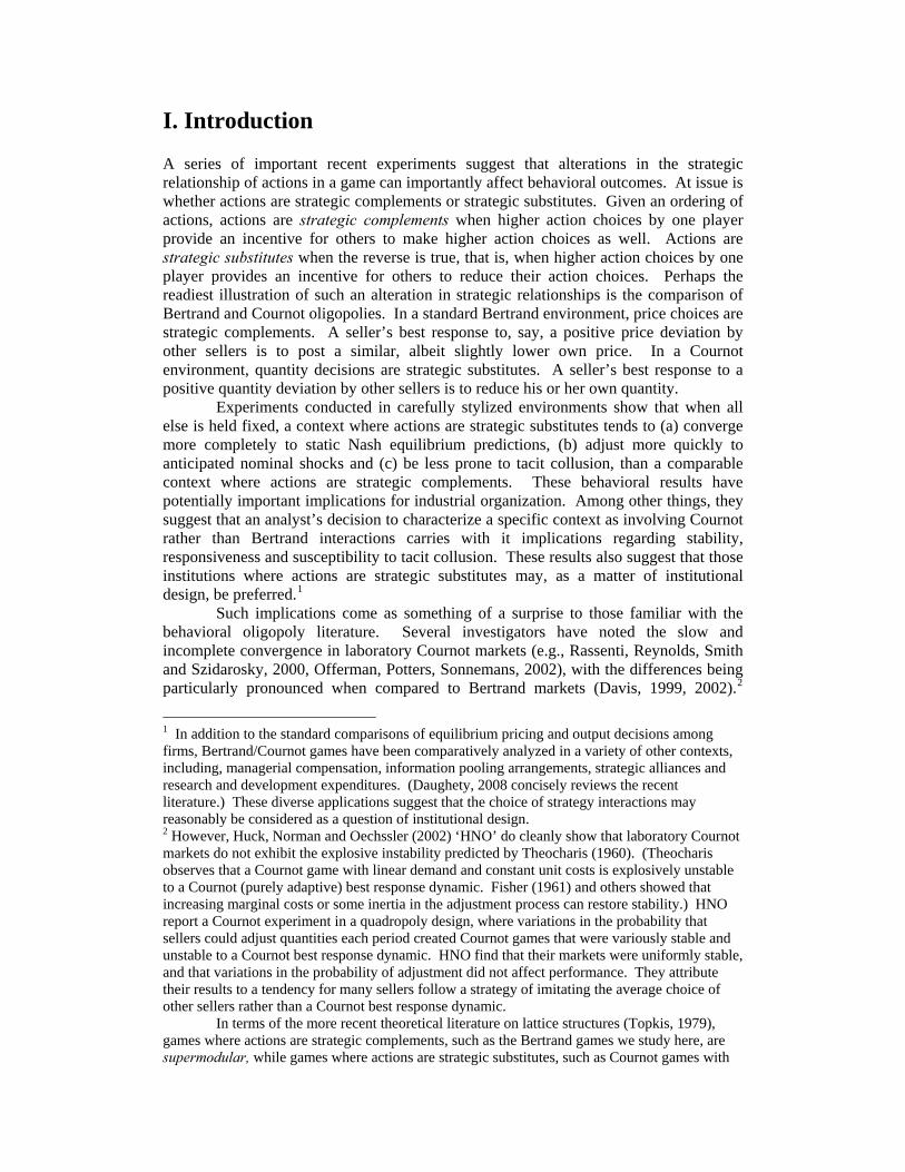
the Bertrand game shown in the upper left panel of Figure 1, a seller with purely adaptive expectations will respond to an announced demand shock that shifts vertically downward the best reply function, by posting price pB. If all sellers are similarly adaptive, this will yield a market price

B

)( BC pp = , leading to a difference between expected and observed prices )( CA pp − . The response of sellers with adaptive expectations to a similar nominal shock in a game where actions are strategic substitutes, such as the Cournot game illustrated in the upper right panel of Figure 1, will lead to the much larger difference, or ‘expectation error’ )( CA qq − . Thus, Fehr and Tyran conclude, when actions are strategic substitutes, adaptive sellers commit larger errors, which stimulate a more rapid adjustment of expectations.

Figure 1. Adaptive Expectations in Bertrand and Cournot Games A third paper suggests that the nature of strategic relations also affects sellers’

propensities to coordinate actions. Potters and Suetens (2008) examine the effects of strategic complements and strategic substitutes on the prevalence of tacit collusion. This experiment consists of a pair of stylized two seller games, presented in a bi-matrix format, where a variety of factors, including the Nash equilibrium, Pareto optimal prices and profits, as well as the absolute slope of the best response functions are held constant across treatments. The primary treatment variable is again the algebraic sign on the best response function slope. Potters and Suetens report average cooperation levels more than twice as large under complementarity than under substitutability. As with HHST and Fehr and Tyran, these investigators explain their results in terms of bounded

Bertrand Game (θ =.5)

p-i

p i

45° line

Best Reply Post Shock

A

B

C

p Ap C

p A

p B

Best Reply Pre Shock

Cournot Game (θ =.5)q i

45 ° lineBest Reply Pre-Shock

Best Reply, Post Shock

A

B

Cq A

q B

q C q A q -i

Bertrand Game (θ =.9)

p -i

p i

45° line

Best Reply Post Shock

a

bc

Best Reply Pre Shock

p b

p a

p c p a

Cournot Game (θ =.9)q i

45 ° lineBest Reply Pre-Shock

Best Reply, Post Shock

q -i

a

b

c

q a

q a

q bT

q cTq c

q b

4

rationality: when actions are strategic complements rather than substitutes, rational players optimize by moving toward the actions of the boundedly rational players. In a repeated context, a tendency to copy the actions of other (high pricing) sellers, not only slows convergence, but, facilitates tacit collusion. 5

Importantly, although none of the above papers are offered explicitly as analyses of Cournot and Bertrand oligopolies, none of the authors exclude Bertrand and Cournot oligopoly from the range of potential applications of their experiment. To the contrary, both Fehr and Tyran (2008) and Potters and Suetens (2008) discuss the comparison between Cournot and Bertrand markets in the development of their experimental designs.6 The highly stylized designs, particularly in these the latter two papers, were developed to isolate the effects of changes in the strategic relations of actions.7

3. A Model of Cournot and Bertrand Interactions In distinction to the papers reviewed in the preceding section, we are interested in assessing the effects of a change in the strategic relations of actions in a standard, repeated market context, an approach that follows a long tradition of laboratory market research investigating the performance of trading institutions (e.g., Holt, 1995). Thus, rather than holding constant everything other than the sign on the slope of the best response function, we vary the form of strategic interactions given a constant demand system and cost structure. This alteration affects a number of factors other than the strategic relation of actions, including the slope of the best response function, the underlying Nash equilibrium prices and quantities, and dynamic incentives to tacitly collude.

To identify these differences, consider a four seller market where each firm produces with no fixed costs and with identical marginal costs, c. Each firm i’s objective function may be written as

iii qcp )( −=π (1)

Where firm i optimizes either pi or qi, depending on the nature of interactions. Assume that each firm produces a distinguishable product, with inverse demand given by

iii qqap −−−= θ3 (2)

5 Recent experimental results by Anderson, Freeborn and Holt (2008) raise some question about this conclusion. These authors vary the strategic relation of actions in a price setting duopoly experiment by varying products from substitutes (making actions strategic complements) to complements (making actions strategic substitutes). Contrary to Potters and Suetens, they find some moderate evidence of tacit collusion when actions are strategic substitutes, but no systematic evidence of tacit collusion when actions are strategic complements. 6 See Fehr and Tyran (2008), note 2, p. 354 and Potters and Suetens (2008), introduction, 3rd paragraph. 7 Fehr and Tyran (2008) indicate that their use of “a price setting game that cannot be derived from usual market structures such as oligopoly or monopolistic competition… does not question the potential importance of our results for behavior outside the laboratory” (note 7, p. 360). Similarly, Potters and Suetens (2008) clearly indicate that oligopoly games fall within the scope application for their results (“It is not only in industrial organization that the prevalence of cooperation may interact.. with strategic complementarity or substitutability.” (3rd para. prior to the end of the introduction, emphasis added.)

5

where iq− is the average quantity choice of the other three sellers, and where θ ∈[0, 1) reflects the substitutability between products, with products becoming perfect substitutes as θ approaches 1.8

For a comparable price setting game, sellers optimize (1) with respect to quantity, a problem which requires solving the demand function in (2) in terms of prices. Solving (2) for quantities yields

iii ppaq −+−= βα 3~ (3)

where ip− is the average price choice of the other players, and where θ31

~+

=aa ,

)31)(1(21

θθθα+−

+= and

)31)(1( θθθβ+−

= . Observe that the restriction 0<θ<1

implies that α >β. To develop static equilibrium price, quantity and profit predictions for the Cournot game, insert (2) into the expression for pi in (1) and optimize. Setting qj = qi and solving yields the symmetric equilibrium quantities, prices and profits,

θ32 +−

=caqc

i (4a)

θθ

32]31[

+++

=capc

n (4b)

and

2

2

)32()(θ

π+−

=cac

N . (4c)

Similarly, static equilibrium price, quantity and profit predictions for the

Bertrand game may be developed by inserting (3) for qi in (1), and optimizing with respect to price. In the symmetric equilibrium, quantities, prices and profits are,

][)31)(2(

21)32

)3(~( cacaqb

n −++

+=

−−+

=θθ

θβααβα (5a)

8 In the experiment that follows, the price space is truncated at unit costs, and the quantity space is truncated at 0. Huck, Normann and Oechssler (2000) show that such truncation of the price and quantity space does not affect equilibrium predictions, and for this reason, we ignore such restrictions in this analysis. We do observe, however, that this (conventional) decision to truncate the implied quantity and price spaces does at least potentially have implications for repeated games. In the Bertrand game, price increases above a seller’s residual demand curve intercept do not affect own sales, but do increase residual demand for each of the other sellers, potentially creating opportunities for inter-period coordination. In the Cournot game, very high quantity postings by a single seller can put all sellers in a range of zero earnings, regardless of individual choices, thus possibly slowing the convergence process. Although we observed no instances of attempted inter-period coordination in our Bertrand markets, in one Cournot market persistently excessive quantity postings by one seller reduced earnings for the other sellers to zero for a significant portion of the session. We discuss this session more fully below.

6

θθθ

βαα

+++−

=−+

=2

)21()1(32

~ cacapbn (5b)

and

222

2

)()31()2(

)1)(21()32(

)3~( caccaBn −

++−+

=−

−+=

θθθθ

βααβαπ , (5c)

where the rightmost terms are Bertrand predictions expressed in terms of Cournot parameters.

Linear Cournot and Bertrand games with constant costs and a given demand system are distinguishable in that the static equilibrium for the Cournot game involves smaller quantities and higher prices (e.g., Vives, 1999). In the above system, this can be seen by comparing equations (4a) and (4b) with the right side of equations (5a) and (5b). For any 0<θ<1, (4a) < (5a), and (4b) >(5b).

The best response functions for Cournot and Bertrand sellers differ in ways that may affect convergence and stability. To see this, generate the best response function for the Cournot game by inserting (2) into the price expression (1). Optimizing with respect to q yields

23

2i

iqcaq −−

−=

θ. (6)

Similarly, generate the best response function for the Bertrand game by inserting (3) into the quantity expression in (1) and optimizing with respect to p.

θθ

θθθ

αβ

αα

423

42)21()1(

23

2

~

++

+++−

=++

= −− iibi

pcapcap (7)

Comparing the slopes of (6) and (7), observe first that the algebraic signs are different, reflecting the strategic substitutability of actions in the Cournot game, in equation (6) and the strategic complementarity of actions in the Bertrand game, in equation (7). Note also that the absolute magnitudes of the best response function slopes also differ across Cournot and Bertrand environments. Taking the ratio of the best response function

slopes in (6) and (7) yields242 θ+

. This ratio can be unitary only when products are

unrelated (e.g., θ=0). As products become better substitutes (e.g., as θ→1) the slope of the Bertrand function becomes relatively flatter. As observed, for example, by Chen and Gazzale (2004, p. 1512), no standard theoretical argument indicates how changes in the slope of the best response affects convergence speeds and levels. However, extension of the ‘endogenous rationality’ argument by Fehr and Tyran, suggests that the relatively steeper reaction function slopes induced by decreased differentiation in Cournot games should enhance relative convergence levels and speeds in Cournot markets. To see this, consider the effects of reducing differentiation from θ=.5, as shown in the upper panels of Figure 1, to θ=.9, illustrated in the lower panels. In Bertrand markets, reduced differentiation cuts the size of the adaptive expectations error from )( CA pp − to )( ca pp − . On the other hand, in the Cournot markets, reduced differentiation moves to the negative domain the optimal response to adaptive expectations (reflecting the explosive instability of such a market to

7

purely adaptive expectations). The size of the error to sellers for holding adaptive expectations increases from )( CA qq − to )( ca qq − .9

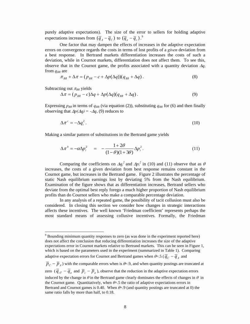
One factor that may dampen the effects of increases in the adaptive expectation errors on convergence regards the costs in terms of lost profits of a given deviation from a best response. In Bertrand markets differentiation increases the costs of such a deviation, while in Cournot markets, differentiation does not affect them. To see this, observe that in the Cournot game, the profits associated with a quantity deviation Δqi from qBR are

)))((( qqqpcp BRBRBR Δ+ΔΔ+−=Δ+ ππ . (8)

Subtracting out πBR yields ))(()( qqqpqcp BRBR Δ+ΔΔ+Δ−=Δπ . (9)

Expressing pBR in terms of qBR (via equation (2)), substituting qBR for (6) and then finally observing that Δp(Δq) = -Δq, (9) reduces to

2i

c qΔ−=Δπ . (10)

Making a similar pattern of substitutions in the Bertrand game yields

22

)31)(1(21

iib pp Δ

+−+

−=Δ−=Δθθ

θαπ . (11)

Comparing the coefficients on Δqi

2 and Δpi2 in (10) and (11) observe that as θ

increases, the costs of a given deviation from best response remains constant in the Cournot game, but increases in the Bertrand game. Figure 2 illustrates the percentage of static Nash equilibrium earnings lost by deviating 5% from the Nash equilibrium. Examination of the figure shows that as differentiation increases, Bertrand sellers who deviate from the optimal best reply forego a much higher proportion of Nash equilibrium profits than do Cournot sellers who make a comparable percentage deviation.

In any analysis of a repeated game, the possibility of tacit collusion must also be considered. In closing this section we consider how changes in strategic interactions affects these incentives. The well known ‘Friedman coefficient’ represents perhaps the most standard means of assessing collusive incentives. Formally, the Friedman

9 Bounding minimum quantity responses to zero (as was done in the experiment reported here) does not affect the conclusion that reducing differentiation increases the size of the adaptive expectations error in Cournot markets relative to Bertrand markets. This can be seen in Figure 1, which is based on the parameters used in the experiment (summarized in Table 1). Comparing adaptive expectation errors for Cournot and Bertrand games when θ=.5 ( AC qq − and

AC pp − ) with the comparable errors when is θ=.9, and when quantity postings are truncated at

zero ( acT qq − and ac pp − ), observe that the reduction in the adaptive expectation errors induced by the change in θ in the Bertrand game clearly dominates the effects of changes in θ in the Cournot game. Quantitatively, when θ=.5 the ratio of adaptive expectations errors in Bertrand and Cournot games is 0.40. When θ=.9 (and quantity postings are truncated at 0) the same ratio falls by more than half, to 0.18.

8

coefficient λ = ND

JPMD

ππππ−−

, where πN denotes static Nash earnings, πJPM denotes

earnings in the joint maximizing outcome, and πD denotes earnings realized by optimally defecting from the joint maximizing outcome. Discount factor λ reflects the minimum probability of continuation necessary to support the joint maximizing outcome as an equilibrium for a repeated game with a threat of permanent reversion to the static Nash equilibrium outcome in response to any deviation. Lower λ’s imply that collusion is easier to support. As indicated by the plot of Friedman Index values for the Cournot and Bertrand games, shown in Figure 3, critical λ values are higher for the Bertrand game than for the comparable Cournot game, with the differences becoming more pronounced as products become closer substitutes. Suetens and Potters (2007) observe higher levels of tacit collusion in Bertrand than in Cournot markets, despite lower λ index values in the Cournot markets, suggesting that when making comparisons across Cournot and Bertrand games, the changes in the nature of strategic interactions dominates the effects change in dynamic incentives implied by lower Friedman coefficient values.

0%

2%

4%

6%

8%

0 1

% o

f Nas

h Eq

uilib

rium

Ear

ning

s

0.5 0.9

Bertrand Market

Cournot Market

Figure 2. Costs of a 5% deviation from the optimal quantity (Cournot) or price (Bertrand) choice, as θ increases, where costs are measured as the percentage of Nash equilibrium earnings lost.

On the other hand, in a price-setting Bertrand-Edgeworth context Davis (2008) reports that variations in the Friedman coefficient are significantly (and inversely) correlated with observed price-cost mark-ups. Davis, however, finds little evidence that sellers engage in the contingent strategy play consistent with the model underlying the Friedman coefficient. Rather, observed price/cost deviations appear to be a consequence of unstructured signaling and response behavior by sellers, the costs of which are driven by excess capacity. Observing a very high correlation between excess capacity and Friedman coefficient values, Davis suggests that the Friedman coefficient is a coincident variable that moves with the drivers of the tacit collusion observed in the laboratory.

In the Bertrand games investigated here, Friedman coefficient values may also move coincidently with tacit collusion, since the costs of deviating from a best response reflect the expected costs of both signaling and response activity. For this reason, we

9

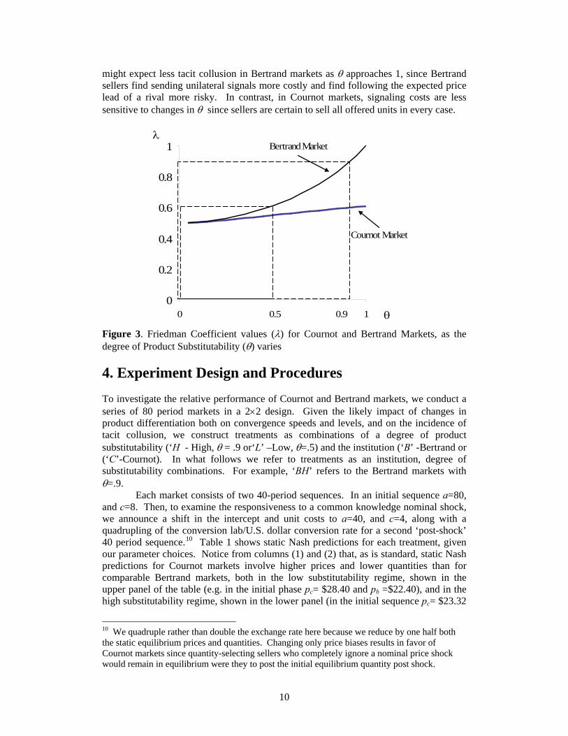
might expect less tacit collusion in Bertrand markets as θ approaches 1, since Bertrand sellers find sending unilateral signals more costly and find following the expected price lead of a rival more risky. In contrast, in Cournot markets, signaling costs are less sensitive to changes in θ since sellers are certain to sell all offered units in every case.

0

0.2

0.4

0.6

0.8

1

0 1

Cournot Market

θ0.90.5

Bertrand Marketλ

Figure 3. Friedman Coefficient values (λ) for Cournot and Bertrand Markets, as the degree of Product Substitutability (θ) varies

4. Experiment Design and Procedures

To investigate the relative performance of Cournot and Bertrand markets, we conduct a series of 80 period markets in a 2×2 design. Given the likely impact of changes in product differentiation both on convergence speeds and levels, and on the incidence of tacit collusion, we construct treatments as combinations of a degree of product substitutability (‘H - High, θ = .9 or‘L’ –Low, θ=.5) and the institution (‘B’ -Bertrand or (‘C’-Cournot). In what follows we refer to treatments as an institution, degree of substitutability combinations. For example, ‘BH’ refers to the Bertrand markets with θ=.9.

Each market consists of two 40-period sequences. In an initial sequence a=80, and c=8. Then, to examine the responsiveness to a common knowledge nominal shock, we announce a shift in the intercept and unit costs to a=40, and c=4, along with a quadrupling of the conversion lab/U.S. dollar conversion rate for a second ‘post-shock’ 40 period sequence.10 Table 1 shows static Nash predictions for each treatment, given our parameter choices. Notice from columns (1) and (2) that, as is standard, static Nash predictions for Cournot markets involve higher prices and lower quantities than for comparable Bertrand markets, both in the low substitutability regime, shown in the upper panel of the table (e.g. in the initial phase pc= $28.40 and pb =$22.40), and in the high substitutability regime, shown in the lower panel (in the initial sequence pc= $23.32

10 We quadruple rather than double the exchange rate here because we reduce by one half both the static equilibrium prices and quantities. Changing only price biases results in favor of Cournot markets since quantity-selecting sellers who completely ignore a nominal price shock would remain in equilibrium were they to post the initial equilibrium quantity post shock.

10

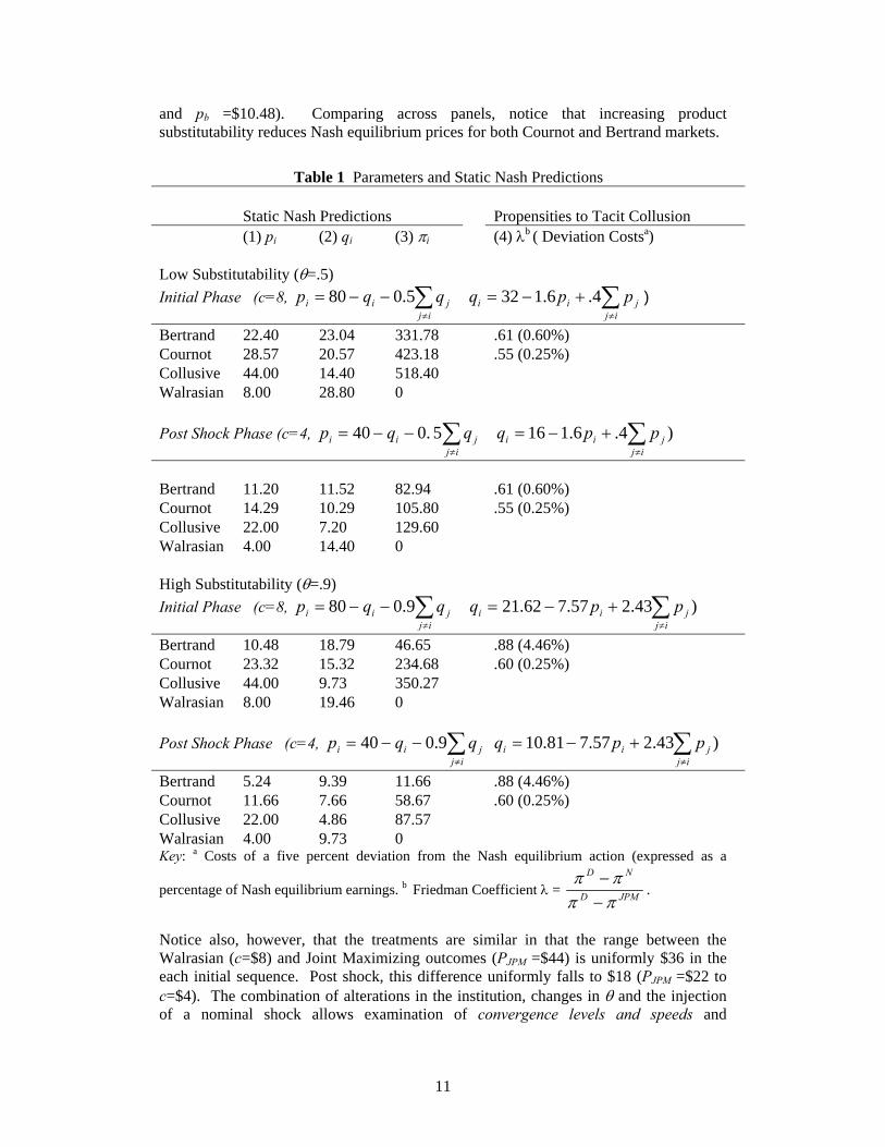
and pb =$10.48). Comparing across panels, notice that increasing product substitutability reduces Nash equilibrium prices for both Cournot and Bertrand markets.

Table 1 Parameters and Static Nash Predictions Static Nash Predictions Propensities to Tacit Collusion (1) pi (2) qi (3) πi (4) λb ( Deviation Costsa) Low Substitutability (θ=.5) Initial Phase (c=8, ∑∑

≠≠

+−=−−=ij

jiiij

jii ppqqqp 4.6.1325.080 )

Bertrand 22.40 23.04 331.78 .61 (0.60%) Cournot 28.57 20.57 423.18 .55 (0.25%) Collusive 44.00 14.40 518.40 Walrasian 8.00 28.80 0 Post Shock Phase (c=4, )4.6.1165.040 ∑∑

≠≠

+−=−−=ij

jiiij

jii ppqqqp

Bertrand 11.20 11.52 82.94 .61 (0.60%)

Cournot 14.29 10.29 105.80 .55 (0.25%) Collusive 22.00 7.20 129.60 Walrasian 4.00 14.40 0 High Substitutability (θ=.9) Initial Phase (c=8, )43.257.762.219.080 ∑∑

≠≠

+−=−−=ij

jiiij

jii ppqqqp

Bertrand 10.48 18.79 46.65 .88 (4.46%) Cournot 23.32 15.32 234.68 .60 (0.25%) Collusive 44.00 9.73 350.27 Walrasian 8.00 19.46 0 Post Shock Phase (c=4, )43.257.781.109.040 ∑∑

≠≠

+−=−−=ij

jiiij

jii ppqqqp

Bertrand 5.24 9.39 11.66 .88 (4.46%) Cournot 11.66 7.66 58.67 .60 (0.25%) Collusive 22.00 4.86 87.57

Key: a Costs of a five percent deviation from the Nash equilibrium action (expressed as a

percentage of Nash equilibrium earnings. b Friedman Coefficient λ = JPMD

ND

ππππ

−−

.

Walrasian 4.00 9.73 0

Notice also, however, that the treatments are similar in that the range between the Walrasian (c=$8) and Joint Maximizing outcomes (PJPM =$44) is uniformly $36 in the each initial sequence. Post shock, this difference uniformly falls to $18 (PJPM =$22 to c=$4). The combination of alterations in the institution, changes in θ and the injection of a nominal shock allows examination of convergence levels and speeds and

11

susceptibility to tacit collusion in Cournot and Bertrand markets. Consider these issues in turn.

4.1 Convergence Levels and Speeds Following the analysis of Chen and Gazzale (2004) we evaluate market convergence in terms of the propensity of agents to make choices within an ε neighborhood of the Nash prediction. One treatment exhibits a higher convergence level than another when the percentage of choices in an ε neighborhood of the Nash prediction over a range of periods exceeds the comparable percentage over the same range for another market. A treatment exhibits a higher convergence speed if the slope of its adjustment path is significantly steeper.

To the extent that shifting actions from strategic substitutes to strategic complements facilitates convergence, as the papers reviewed in Section 2 suggest, we should observe higher convergence levels and speeds in Cournot markets than in Bertrand markets. This is a first conjecture.

Conjecture 1: Convergence levels and speeds are higher in Cournot markets than in comparable Bertrand markets.

To the extent that the size of adaptive expectations errors in a given context endogenously affects rationality (as Fehr and Tyran suggest), we should also observe relatively higher convergence levels and speeds in Cournot markets as θ increases. This is a second conjecture.

Conjecture 2: The superiority of convergence levels and speeds in Cournot markets relative to Bertrand markets increases as the rate of product substitutability increases from θ=.5 to θ=.9. Evaluation of seller responses to our announced nominal shock will allow a most direct comparison with results in Fehr and Tyran (2008). 4.2. Tacit Collusion Results by Potters and Suetens (2008) suggest that all else equal, a context where actions are strategic complements rather than strategic substitutes facilitates tacit collusion. To the extent that this result extends to our comparison of Bertrand and Cournot quadropolies, we should expect more tacit collusion in Bertrand markets than in Cournot markets. This is a third conjecture. Conjecture 3. Tacit collusion, measured as the mean deviation from the static Nash equilibrium price, is higher in Bertrand markets than in Cournot markets.

As discussed above, however, the relative propensity toward tacit collusion may

not be independent of the degree of product differentiation. As products become closer substitutes, the relative costs of signaling and response behavior increases in Bertrand games. Thus, as θ increases, we would expect relatively less tacit collusion in Bertrand environments. This is a fourth and final conjecture.

12

Conjecture 4, Increasing the rate of substitutability from θ=.5 to θ=.9 reduces the incidence of tacit collusion in Bertrand games relative to Cournot games. 4.3. Experiment Procedures At the start of each session, participants are randomly seated at visually isolated computer terminals. After seating, a monitor reads instructions aloud as participants follow along on copies of their own. The instructions explain that each period sellers simultaneously submit a price (quantity) decision, as well as a forecast of others’ mean price (quantity) choices. Forecasts are submitted under the condition that sellers will earn a small ‘forecasting prize’ each period the forecast is sufficiently accurate.11 Once all decisions are complete, an automated buyer makes purchase decisions in accordance with one of the demand conditions shown in Table 1. At the end of each trading period, participants receive as feedback the average price (quantity) choice of the other sellers, whether or not they won the forecast prize, and their own earnings, both for the period, and cumulatively.

In addition to explaining the price (quantity) posting and feedback procedures, instructions present to sellers as common information demand and underlying cost conditions as well as the number of periods in the each sequence. To help them better understand their induced demand condition we gave participants a profit calculator that allowed them to evaluate the earnings consequences of hypothetical own and average others’ action choices.

After giving participants an opportunity to privately ask any questions they might have, a first 40 period sequence begins, in the initial high demand/ high cost condition. Following the conclusion of the first sequence, participants are handed a piece of paper that presents demand and cost conditions for the post-shock environment as well as a new Lab/U.S. currency conversion rate that keeps equilibrium earnings equal across the initial post-shock environments. Pertinent parameters in their profit calculators are also updated. The experiment then continues for another forty periods. Following the second sequence participants are privately paid the sum of their earnings from the two sequences plus a $6 appearance fee, and dismissed one at a time.

In total we conducted six markets in each treatment cell, for a total of 24 market sessions. Participants were 96 undergraduate students enrolled in upper level business courses at Virginia Commonwealth University in the spring semester of 2008. No participant had previous experience with a linear oligopoly market, and no one participated in more than a single session. Conversion rates were varied across treatments in order to hold expected payoffs roughly constant across treatments. In the θ=.5 condition we used a conversion rate 1800 lab dollars = $1 U.S. in the Cournot markets and 1400 lab dollars to $1 U.S. in the Bertrand markets. When θ=.9, lab dollar earnings were converted to U.S. currency at a rate of $1000 = $1 U.S. in the Cournot

11 ‘Accurate’ is within $0.30 of the subsequently observed others’ mean price choice in the Bertrand markets and within 0.20 units of the subsequently observed others’ mean quantity choice the Cournot markets. The narrower range for the forecasting game in the Cournot markets reflects the narrower effective choice space in those markets, as can be seen by comparing the price and quantity differences between Walrasian and Collusive outcomes Table 1. The size of the forecasting prize was also varied across treatments to maintain an approximately constant absolute and relative saliency of the prize across treatments. With θ=.9 the per period forecast prize was 10 lab dollars in both the Bertrand and Cournot games. With θ=.5, the per period forecast prize was 1 lab dollar in the Bertrand game and 5 lab dollars in the Cournot game.

13

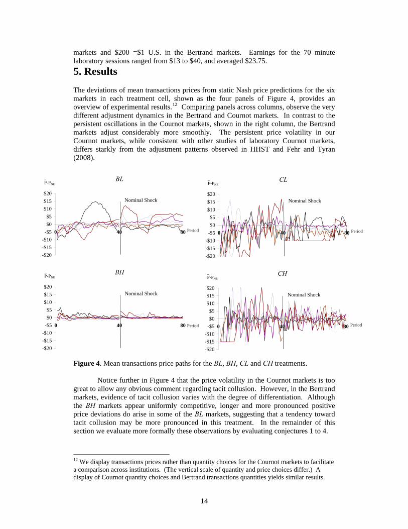
markets and $200 =$1 U.S. in the Bertrand markets. Earnings for the 70 minute laboratory sessions ranged from $13 to $40, and averaged $23.75. 5. Results The deviations of mean transactions prices from static Nash price predictions for the six markets in each treatment cell, shown as the four panels of Figure 4, provides an overview of experimental results.12 Comparing panels across columns, observe the very different adjustment dynamics in the Bertrand and Cournot markets. In contrast to the persistent oscillations in the Cournot markets, shown in the right column, the Bertrand markets adjust considerably more smoothly. The persistent price volatility in our Cournot markets, while consistent with other studies of laboratory Cournot markets, differs starkly from the adjustment patterns observed in HHST and Fehr and Tyran (2008).

BH

-$20-$15-$10

-$5$0$5

$10$15$20

0 40 80

P-PNE

Period

Nominal Shock

_

.

BL

-$20-$15-$10

-$5$0$5

$10$15$20

0 40 80

P-PNE

Period

Nominal Shock

_

.

CH

-$20-$15-$10

-$5$0$5

$10$15$20

0 40

P-PNE

Period80

Nominal Shock

_

.

CL

-$20-$15-$10

-$5$0$5

$10$15$20

0 40

P-PNE

Period80

Nominal Shock

_

.

Figure 4. Mean transactions price paths for the BL, BH, CL and CH treatments.

Notice further in Figure 4 that the price volatility in the Cournot markets is too great to allow any obvious comment regarding tacit collusion. However, in the Bertrand markets, evidence of tacit collusion varies with the degree of differentiation. Although the BH markets appear uniformly competitive, longer and more pronounced positive price deviations do arise in some of the BL markets, suggesting that a tendency toward tacit collusion may be more pronounced in this treatment. In the remainder of this section we evaluate more formally these observations by evaluating conjectures 1 to 4. 12 We display transactions prices rather than quantity choices for the Cournot markets to facilitate a comparison across institutions. (The vertical scale of quantity and price choices differ.) A display of Cournot quantity choices and Bertrand transactions quantities yields similar results.

14

5.1 Convergence

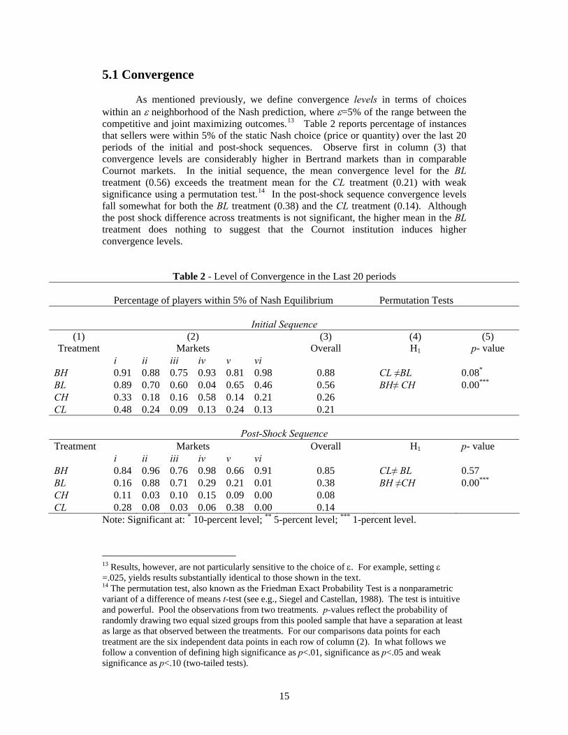
As mentioned previously, we define convergence levels in terms of choices within an ε neighborhood of the Nash prediction, where ε=5% of the range between the competitive and joint maximizing outcomes.13 Table 2 reports percentage of instances that sellers were within 5% of the static Nash choice (price or quantity) over the last 20 periods of the initial and post-shock sequences. Observe first in column (3) that convergence levels are considerably higher in Bertrand markets than in comparable Cournot markets. In the initial sequence, the mean convergence level for the BL treatment (0.56) exceeds the treatment mean for the CL treatment (0.21) with weak significance using a permutation test.14 In the post-shock sequence convergence levels fall somewhat for both the BL treatment (0.38) and the CL treatment (0.14). Although the post shock difference across treatments is not significant, the higher mean in the BL treatment does nothing to suggest that the Cournot institution induces higher convergence levels.

Table 2 - Level of Convergence in the Last 20 periods Percentage of players within 5% of Nash Equilibrium Permutation Tests

Initial Sequence (1)

Treatment (2)

Markets (3)

Overall (4) H1

(5) p- value

i ii iii iv v vi BH 0.91 0.88 0.75 0.93 0.81 0.98 0.88 CL ≠BL 0.08*

BL 0.89 0.70 0.60 0.04 0.65 0.46 0.56 BH≠ CH 0.00***

CH 0.33 0.18 0.16 0.58 0.14 0.21 0.26 CL 0.48 0.24 0.09 0.13 0.24 0.13 0.21

Post-Shock Sequence

Treatment Markets Overall H1 p- value i ii iii iv v vi BH 0.84 0.96 0.76 0.98 0.66 0.91 0.85 CL≠ BL 0.57 BL 0.16 0.88 0.71 0.29 0.21 0.01 0.38 BH ≠CH 0.00***

CH 0.11 0.03 0.10 0.15 0.09 0.00 0.08 CL 0.28 0.08 0.03 0.06 0.38 0.00 0.14

Note: Significant at: * 10-percent level; ** 5-percent level; *** 1-percent level.

13 Results, however, are not particularly sensitive to the choice of ε. For example, setting ε =.025, yields results substantially identical to those shown in the text. 14 The permutation test, also known as the Friedman Exact Probability Test is a nonparametric variant of a difference of means t-test (see e.g., Siegel and Castellan, 1988). The test is intuitive and powerful. Pool the observations from two treatments. p-values reflect the probability of randomly drawing two equal sized groups from this pooled sample that have a separation at least as large as that observed between the treatments. For our comparisons data points for each treatment are the six independent data points in each row of column (2). In what follows we follow a convention of defining high significance as p<.01, significance as p<.05 and weak significance as p<.10 (two-tailed tests).

15

Increasing θ to 0.9 makes convergence levels in the Bertrand markets clearly higher. In the initial sequence the difference in convergence levels across the BH treatment (0.88) and the CH treatment (.26) is a highly significant 0.62. Post shock the difference between BH (.85) and CH (.08) treatment increases to a highly significant 0.77.

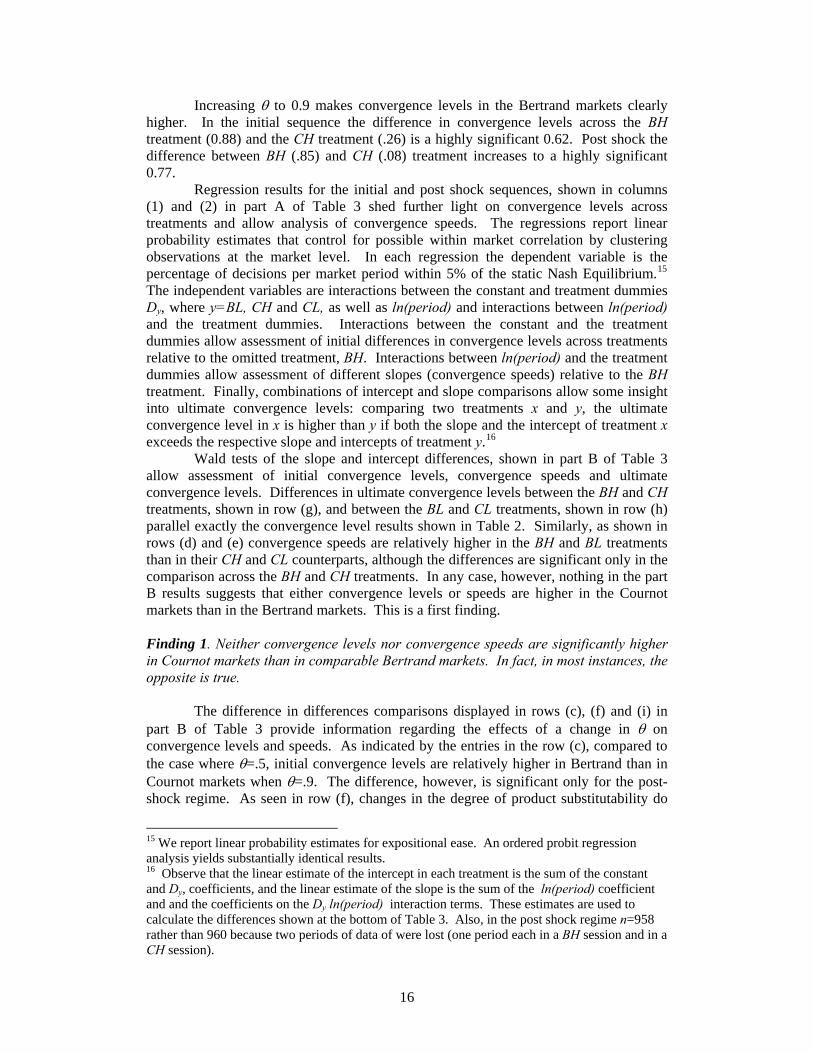
Regression results for the initial and post shock sequences, shown in columns (1) and (2) in part A of Table 3 shed further light on convergence levels across treatments and allow analysis of convergence speeds. The regressions report linear probability estimates that control for possible within market correlation by clustering observations at the market level. In each regression the dependent variable is the percentage of decisions per market period within 5% of the static Nash Equilibrium.15 The independent variables are interactions between the constant and treatment dummies Dy, where y=BL, CH and CL, as well as ln(period) and interactions between ln(period) and the treatment dummies. Interactions between the constant and the treatment dummies allow assessment of initial differences in convergence levels across treatments relative to the omitted treatment, BH. Interactions between ln(period) and the treatment dummies allow assessment of different slopes (convergence speeds) relative to the BH treatment. Finally, combinations of intercept and slope comparisons allow some insight into ultimate convergence levels: comparing two treatments x and y, the ultimate convergence level in x is higher than y if both the slope and the intercept of treatment x exceeds the respective slope and intercepts of treatment y.16

Wald tests of the slope and intercept differences, shown in part B of Table 3 allow assessment of initial convergence levels, convergence speeds and ultimate convergence levels. Differences in ultimate convergence levels between the BH and CH treatments, shown in row (g), and between the BL and CL treatments, shown in row (h) parallel exactly the convergence level results shown in Table 2. Similarly, as shown in rows (d) and (e) convergence speeds are relatively higher in the BH and BL treatments than in their CH and CL counterparts, although the differences are significant only in the comparison across the BH and CH treatments. In any case, however, nothing in the part B results suggests that either convergence levels or speeds are higher in the Cournot markets than in the Bertrand markets. This is a first finding.

Finding 1. Neither convergence levels nor convergence speeds are significantly higher in Cournot markets than in comparable Bertrand markets. In fact, in most instances, the opposite is true.

The difference in differences comparisons displayed in rows (c), (f) and (i) in part B of Table 3 provide information regarding the effects of a change in θ on convergence levels and speeds. As indicated by the entries in the row (c), compared to the case where θ=.5, initial convergence levels are relatively higher in Bertrand than in Cournot markets when θ=.9. The difference, however, is significant only for the post-shock regime. As seen in row (f), changes in the degree of product substitutability do

15 We report linear probability estimates for expositional ease. An ordered probit regression analysis yields substantially identical results. 16 Observe that the linear estimate of the intercept in each treatment is the sum of the constant and Dy, coefficients, and the linear estimate of the slope is the sum of the ln(period) coefficient and and the coefficients on the Dy ln(period) interaction terms. These estimates are used to calculate the differences shown at the bottom of Table 3. Also, in the post shock regime n=958 rather than 960 because two periods of data of were lost (one period each in a BH session and in a CH session).

16

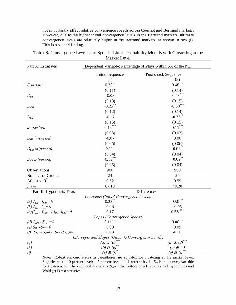
not importantly affect relative convergence speeds across Cournot and Bertrand markets. However, due to the higher initial convergence levels in the Bertrand markets, ultimate convergence levels are relatively higher in the Bertrand markets, as shown in row (i). This is a second finding.

Table 3. Convergence Levels and Speeds: Linear Probability Models with Clustering at the Market Level

Part A: Estimates Dependent Variable: Percentage of Plays within 5% of the NE

Initial Sequence Post shock Sequence (1) (2) Constant 0.25** 0.48***

(0.11) (0.14) DBL -0.08 -0.44***

(0.13) (0.15) DCH -0.25** -0.50***

(0.12) (0.14) DCL -0.17 -0.38**

(0.15) (0.15) ln (period) 0.18*** 0.11***

(0.03) (0.03) DBL ln(period) -0.07 0.00 (0.05) (0.06) DCH ln(period) -0.11** -0.08**

(0.04) (0.04) DCL ln(period) -0.15*** -0.09**

(0.05) (0.04) Observations 960 958 Number of Groups 24 24 Adjusted R2 0.52 0.59 F(3,23) 67.13 48.28

Part B: Hypothesis Tests Differences Intercepts (Initial Convergence Levels)

(a) IBH - ICH =0 0.25** 0.50***

(b) IBL - ICL=0 0.08 -0.05 (c)(IBH - ICH) –( IBL -ICL)=0 0.17 0.55 ***

Slopes (Convergence Speeds) (d) SBH - SCH =0 0.11*** 0.08 **

(e) SBL -SCL=0 0.08 0.09 (f) (SBH - SCH) -( SBL -SCL)=0 0.03 -0.01

Intercepts and Slopes (Ultimate Convergence Levels) (g) (a) & (d)*** (a) & (d)***

(h) (b) & (e)**

Notes: Robust standard errors in parentheses are adjusted for clustering at the market level. Significant at * 10 percent level; ** 5 percent level, *** 1 percent level. Dy is the dummy variable for treatment y. The excluded dummy is DBH. The bottom panel presents null hypotheses and Wald χ2(1) test statistics.

(b) & (e) (i) (c) & (f)* (c) & (f)***

17

Finding 2. Increasing substitutability does not significantly affect convergence speeds in Bertrand markets relative to Cournot market but does improve convergence levels. Findings 1 and 2 run flatly counter to results by Fehr and Tyran (2008). In particular, focusing on the post shock sequence, we observe that the Cournot markets here not only fail to respond significantly more quickly and completely to an announced shock than comparable Bertrand markets, but they respond more slowly and less completely. Further, contrary to the reasoning offered by Fehr and Tyran, these differences worsen as the products become closer substitutes (and the size of an error in expectations increases). We consider possible reasons for our results in the next section. First, however, we consider results regarding tacit collusion. 5.3 Tacit Collusion Potters and Suetens (2008) and others assess the propensity for tacit collusion in terms of a cooperation index, where the degree of cooperation in a market k for a period t is defined as

NashJPM

Nashkt

kt choicechoicechoicechoiceaverage

−−

=φ .

Table 4 lists average cooperation index values for both the last 20 periods of the initial and post-shock phases of each session. Notice from the treatment means shown in column (3) of the Table that when products are close substitutes, cooperativeness levels are nearly zero in both the Cournot and Bertrand markets. In the initial sequence BHφ =

-0.01 and CHφ = 0.00. Post shock these numbers remain near zero, BHφ = 0.00 and

CHφ = -0.02. As indicated by the permutation test results shown in column (5), these differences do not approach significance. When θ = .5 deviations from cooperation levels the BL treatment very modestly exceed those in the counterpart CL treatment ( BLφ

= 0.05 and CLφ = 0.01). Post shock, differences in cooperation levels increase

substantially ( BLφ = 0.13 and CLφ = -0.48), and, as indicated by permutation test results in column (5), this difference is weakly significant. These observations yield our third and fourth findings. Finding 3. Tacit collusion is not uniformly more pervasive in Bertrand Markets than in Cournot Markets. When θ=.9 the effects of tacit collusion are no more pronounced in Bertrand markets than in Cournot markets. Finding 4. Reducing substitutability from θ=.9 to θ=.5 increases the incidence of tacit collusion in Bertrand markets relative to Cournot markets. Finding 3 casts some doubt on the generality of the conclusion by Potters and Suetens (2008) that markets with strategic complements are more susceptible to tacit collusion than markets with strategic complements. Finding 4, however, suggests that at least in some contexts Bertrand markets, even those with four sellers, may be relatively more

18

susceptible to tacit collusion.17 Notice, in particular under column (2) of Table 4, that the bulk of large positive deviations arise in the BL markets: four of the five session segments with φ>.20 occurred in the BL treatment (entries are bolded for emphasis). In closing this section, we consider the kinds of seller behaviors that drive instances of supra-competitive outcomes.

Table 4 – Degree of Cooperation -Last 20 periods φk treatmentφ Permutation Tests

Initial Sequence

(1) Treatment

(2) Markets

(3) Overall

(4) H1

(5) p- value

i ii iii iv v vi BH -0.03 0.00 -0.02 0.02 -0.02 0.02 -0.01 BL≠CL 1.00 BL 0.03 -0.06 -0.02 0.34 0.00 0.03 0.05 BH≠CH 1.00 CH 0.02 0.05 -0.13 -0.01 -0.05 0.10 0.00 CL 0.04 0.03 -0.28 -0.13 -0.08 0.49 0.01

Post-Shock Sequence

i ii iii iv v vi BH -0.01 -0.01 -0.04 0.02 0.00 0.02 0.00 BL≠CL 0.08*

BL 0.23 -0.03 -0.08 -0.16 0.24 0.58 0.13 BH≠CH 1.00 CH 0.07 -0.05 0.00 -0.06 0.04 -0.13 -0.02 CL -0.25 -0.33 -0.69 0.02 -0.09 -1.56 -0.48

Notes: 20

20∑−= −

−

=

y

ytNashJPM

Nsahkt

kchoicechoice

choicechoiceaverage

φ .where y= the final period for a sequence

k (e.g., period 40 or period 80). Bolded entries highlight instances where φk>.20

As a first observation, we observe that nothing obvious in the price or quantity decisions for these market segments suggests that sellers coordinated their actions. Sellers, for example, never posted the same price in any period of the Bertrand markets, and only selected the same quantity in one period of the Cournot markets.18 Sellers do, however, differ across treatments with respect to signaling behavior. It is useful to divide signals into two types: ‘spikes’ which are large, single period price or quantity deviations, and ‘surges,’ or a series of smaller but repeated deviations. More precisely

17 However, we also note that much of the difference in observed mean cooperation rates across the BL and CL treatments is driven by overly-competitive behavior in the Cournot markets rather than by high levels of cooperation in the Bertrand markets. The cooperation levels observed here in our quadropoly markets is far below that observed in the duopoloies reported by Potters and Suetens (2008). Over the last half of the periods in their markets Potters and Suetens observe φ =0.27 in their strategic substitutes treatment and φ =0.51 in their strategic complements treatment. 18 Similarly, sellers never attempted to rotate sales across periods in either the Bertrand or Cournot markets. We suspect that the failure of laboratory sellers to coherently organize tacitly collusive arrangements is fairly typical. Davis (2007) makes similar observations regarding seller behavior in the a Bertrand-Edgeworth pricing game.

19

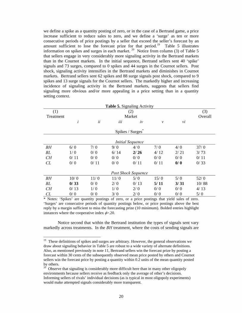
we define a spike as a quantity posting of zero, or in the case of a Bertrand game, a price increase sufficient to reduce sales to zero, and we define a ‘surge’ as ten or more consecutive periods of price postings by a seller that exceed the seller’s forecast by an amount sufficient to lose the forecast prize for that period.19 Table 5 illustrates information on spikes and surges in each market. 20 Notice from column (3) of Table 5 that sellers engage in very considerably more signaling activity in the Bertrand markets than in the Cournot markets. In the initial sequence, Bertrand sellers sent 40 ‘spike’ signals and 73 surges, compared to 0 spikes and 44 surges in the Cournot sellers. Post shock, signaling activity intensifies in the Bertrand markets and diminishes in Cournot markets. Bertrand sellers sent 62 spikes and 88 surge signals post shock, compared to 9 spikes and 13 surge signals for the Cournot sellers. The markedly higher and increasing incidence of signaling activity in the Bertrand markets, suggests that sellers find signaling more obvious and/or more appealing in a price setting than in a quantity setting context.

Table 5. Signaling Activity

(1) Treatment

(2) Market

(3) Overall

i ii iii iv v vi

Spikes / Surges*

Initial Sequence

BH 6/ 0 7/ 0 9/ 0 4/ 0 7/ 0 4/ 0 37/ 0 BL 1/ 0 0/ 0 6/ 14 2/ 26 4/ 12 2/ 21 3/ 73 CH 0/ 11 0/ 0 0/ 0 0/ 0 0/ 0 0/ 0 0/ 11 CL 0/ 0 0/ 11 0/ 0 0/ 11 0/ 11 0/ 0 0/ 33

Post Shock Sequence BH 10/ 0 11/ 0 11/ 0 5/ 0 15/ 0 5/ 0 52/ 0 BL 0/ 33 0/ 0 2/ 0 0/ 13 5/ 11 3/ 31 10/ 88 CH 0/ 13 1/ 0 1/ 0 2/ 0 0/ 0 0/ 0 4/ 13 CL 0/ 0 0/ 0 3/ 0 2/ 0 0/ 0 0/ 0 5/ 0

* Notes: ‘Spikes’ are quantity postings of zero, or a price postings that yield sales of zero. ‘Surges’ are consecutive periods of quantity postings below, or price postings above the best reply by a margin sufficient to miss the forecasting prize (10 minimum). Bolded entries highlight instances where the cooperative index φ>.20.

Notice second that within the Bertrand institution the types of signals sent vary

markedly across treatments. In the BH treatment, where the costs of sending signals are

19 These definitions of spikes and surges are arbitrary. However, the general observations we draw about signaling behavior in Table 5 are robust to a wide variety of alternate definitions. Also, as mentioned previously in note 11, Bertrand sellers win the forecast prize by posting a forecast within 30 cents of the subsequently observed mean price posted by others and Cournot sellers win the forecast price by posting a quantity within 0.2 units of the mean quantity posted by others. 20 Observe that signaling is considerably more difficult here than in many other oligopoly environments because sellers receive as feedback only the average of other’s decisions. Informing sellers of rivals’ individual decisions (as is typical in most oligopoly experiments) would make attempted signals considerably more transparent.

20

quite high, sellers tend to send one-off price ‘spikes’ with frequency. By way of contrast, in the BL treatment, sellers send relatively few ‘spikes’ but instead tend to engage in smaller, but more persistent price increases.

Observe finally the bolded entries in Table 5, which highlight markets with cooperation index values of φ= .20 or higher. In the Bertrand markets, the bolded entries uniformly exhibit high levels of surge activity, but relatively few spikes. Simple correlations of cooperation index values with surge and spike activity across all Bertrand markets provides further support for the hypothesis that surges rather than spikes tend to raise prices in Bertrand markets. For cooperation values and surges the simple correlation ρ =.72 (p<.0001) is high and significant. For cooperation values and spikes the simple correlation ρ= -0.18 (p< 0.41) is small and not significantly different from zero.

In the Cournot markets, instances of both signaling activity and cooperation index values are lower. As can be seen in Table 5 neither surge nor spike activity occurred in the single (bolded) instance where φ>.20, the initial segment of market CL-vi. To the contrary, the apparently collusive activity in the end of the first sequence of this session appears to be driven by a dramatic swing in quantity choices for an (apparently confused) single seller who posted very large quantities in the initial periods of the session (and who subsequently returned to very large quantity postings in the last half of the session.) For the Cournot markets combined, simple correlations between spike activity and cooperation index values (ρ = -.15, p<0.47) and between surge activity and cooperation index values (ρ = .15, p<0.47) are both small and not significantly different from zero.

In sum, although sample sizes here are relatively small, examination of signaling behavior suggests both why lower levels of cooperative are observed here than in the duopolies reported by Potters and Suetens (2008), and how product substitutability affects cooperativeness. Despite the fact that signaling costs are lower in Cournot markets than in Bertrand markets, signaling activity tends to be higher in Bertrand markets because price signaling intentions are more easily communicated in these relatively stable markets. Nevertheless, even in price setting games, cooperation is fairly difficult with four sellers, and only signals in the form of extensively repeated price surges effectively raise prices. As products become close substitutes, the costs of surge activity become prohibitively high, yielding persistently competitive outcomes. 6. Bounded Rationality and Market Convergence

Our findings regarding the relatively slower convergence speeds and levels in Cournot markets run precisely counter to those by HSST (2007) and particularly Fehr and Tyran (2008). This section explores more fully possible reasons for this result. For specificity and for comparability with the analysis in Fehr and Tyran (2008) we focus primarily on behavior in the post-shock sequence.

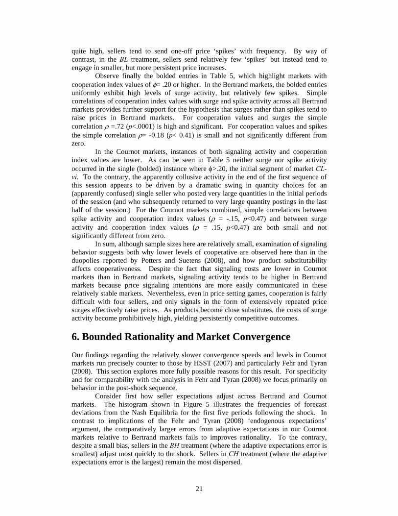
Consider first how seller expectations adjust across Bertrand and Cournot markets. The histogram shown in Figure 5 illustrates the frequencies of forecast deviations from the Nash Equilibria for the first five periods following the shock. In contrast to implications of the Fehr and Tyran (2008) ‘endogenous expectations’ argument, the comparatively larger errors from adaptive expectations in our Cournot markets relative to Bertrand markets fails to improves rationality. To the contrary, despite a small bias, sellers in the BH treatment (where the adaptive expectations error is smallest) adjust most quickly to the shock. Sellers in CH treatment (where the adaptive expectations error is the largest) remain the most dispersed.

21

θ=.9

0%

10%

20%

30%

40%

50%

-10 -9 -8 -7 -6 -5 -4 -3 -2 -1 0 1 2 3 4 5 6 7 8 9 10 >10.5

Range Midpoint - $ (Bertrand) or Units (Cournot)

BHCH

Freq

uenc

y

θ=.5

0%

10%

20%

30%

40%

50%

-10 -9 -8 -7 -6 -5 -4 -3 -2 -1 0 1 2 3 4 5 6 7 8 9 10 >10.5

Range Midpoint- $ (Bertrand) or Units (Cournot)

BLCL

Freq

uenc

y

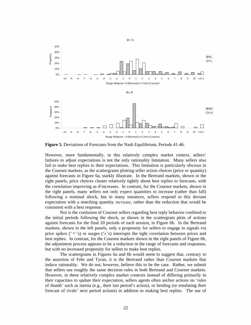
Figure 5. Deviations of Forecasts from the Nash Equilibrium, Periods 41-46. However, more fundamentally, in this relatively complex market context, sellers’ failures to adjust expectations is not the only rationality limitation. Many sellers also fail to make best replies to their expectations. This limitation is particularly obvious in the Cournot markets, as the scattergrams plotting seller action choices (price or quantity) against forecasts in Figure 6a, starkly illustrate. In the Bertrand markets, shown in the right panels, price choices cluster relatively tightly about best replies to forecasts, with the correlation improving as θ increases. In contrast, for the Cournot markets, shown in the right panels, many sellers not only expect quantities to increase (rather than fall) following a nominal shock, but in many instances, sellers respond to this deviant expectation with a matching quantity increase, rather than the reduction that would be consistent with a best response.

Nor is the confusion of Cournot sellers regarding best reply behavior confined to the initial periods following the shock, as shown in the scattergram plots of actions against forecasts for the final 20 periods of each session, in Figure 6b. In the Bertrand markets, shown in the left panels, only a propensity for sellers to engage in signals via price spikes (‘ ’s) or surges (‘×’s) interrupts the tight correlation between prices and best replies. In contrast, for the Cournot markets shown in the right panels of Figure 6b, the adjustment process appears to be a reduction in the range of forecasts and responses, but with no increased propensity for sellers to make best replies.

The scattergrams in Figures 6a and 6b would seem to suggest that, contrary to the assertion of Fehr and Tyran, it is the Bertrand rather than Cournot markets that induce rationality. We do not, however, believe this to be the case. Rather, we submit that sellers use roughly the same decision rules in both Bertrand and Cournot markets. However, in these relatively complex market contexts instead of differing primarily in their capacities to update their expectation, sellers agents often anchor actions on ‘rules of thumb’ such as inertia (e.g., their last period’s action), or herding (or emulating their forecast of rivals’ next period actions) in addition to making best replies. The use of

22

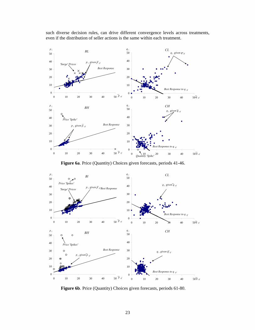
such diverse decision rules, can drive different convergence levels across treatments, even if the distribution of seller actions is the same within each treatment.

Figure 6a. Price (Quantity) Choices given forecasts, periods 41-46.

0

10

20

30

40

50

0 10 20 30 40 50

p i

p -if

Bl

Best Responsep i given p -if 'Surge' Prices

Price 'Spikes'

0

10

20

30

40

50

0 10 20 30 40 50q -if

CLq i

Best Response to q -if

q i given q -if

0

10

20

30

40

50

0 10 20 30 40 50

p i

p -if

BH

Best Response

p i given p -if

Price 'Spikes'

0

10

20

30

40

50

0 10 20 30 40 50 q -if

CHq i

Best Response to q -if

q i given q -if

0

10

20

30

40

50

0 10 20 30 40 50

p i

p -if

BL

Best Response

p i given p -if 'Surge' Prices

0

10

20

30

40

50

0 10 20 30 40 50q -if

CLq i

Best Response to q -if

q i given q -if

0

10

20

30

40

50

0 10 20 30 40 50

p i

p -if

BH

Best Responsep i given p -if

Price 'Spike'

0

10

20

30

40

50

0 10 20 30 40 50 q -if

CHq i

Best Response to q -if

q i given q -if

Quantity 'Spike'

Figure 6b. Price (Quantity) Choices given forecasts, periods 61-80.

23

To understand this point, consider again seller responses to a nominal shock, shown in Figure 1. Suppose that in addition to making a best response, sellers in some instances use their last period action as a reference point for action. (We focus on an ‘inertia’ anchor here, as it is easier to unambiguously illustrate than a forecast anchor.) In the case of low differentiation (θ =.5), shown in the upper half of Figure 1, the variation in price choices that these two rules imply in the Bertrand game is smaller than the variation in quantity choices that these rules imply for the Cournot game . Turning to the lower panel, observe that as differentiation increases (θ =.9), this range in outcomes falls from

)( BA pp −

)( BA qq −)( BA pp − to )( ba pp − in Bertrand markets

but in Cournot markets remains relatively constant at )( BA qq − vs. 21)( ba qq − For this reason, we submit that Bertrand markets, particularly those Bertrand markets in the BH treatment might exhibit less outcome variability, even if sellers used the same mix of best reply and inertia anchors.22

A summary of observed seller actions in terms of best reply, inertia and forecast rules, shown in Table 6, provides some behavioral support for this hypothesis. Columns (1) to (3) on the left side of the Table, list the absolute proximity of seller action choices to best reply, forecast and inertia rules, where we define ‘close’ as an action choice that deviates from the best reply by an amount less than needed to win the forecast prize for the period. Inspection of action rates absolutely close to best replies, listed in column (1) gives the impression that Bertrand markets facilitate best reply behavior, particularly when θ=.9. For example, in the first five periods following the shock, 38% of price choices in the BH treatment and 13% of price choices in the BL treatment were ‘close’ to the best reply. In contrast, only 3% of quantity choices were similarly close to the best reply in either the CH or CL treatments. Bertrand markets remain similarly superior when the basis of comparison is expanded to all 40 periods of the second sequence, as shown in the entries in column (1) in the bottom panel of Table 6. However, as choice rates for forecast and inertia rules, in columns (2) and (3) indicate, the apparently superior performance of the Bertrand markets is driven largely by the overlap of best reply choices and actions consistent with these rules of thumb.

In fact, sellers used roughly the same distribution of best reply, inertia and forecast anchors in each treatment, as can be seen in columns (4) to (6) in Table 6, which enumerates the percentage of instances where actions are relatively closest to best reply, forecast and inertia rules. As inspection of these columns indicates, the relative 21 Truncation of quantity postings to zero does not alter the conclusion that increasing differentiation reduces the range between inertial and pure adaptive best reply response in Bertrand markets relative to Cournot markets. As comparison of the relative differences in prices and quantity postings in the upper and lower panels of Figure 1 suggest, the reduction in the difference between inertial and adaptive prices in the Bertrand markets (pa-pb vs. pA-pB ) dominates the effect of truncating quantity postings to zero (qa-qbT vs. qA-qB). Quantitatively, when θ=.5 the ratio (pA-pB) / (qA-qB ) = 0.39. When θ=.9 the comparable ratio (pa-pb) / (qa-qbT ) =0.18. 22 As mentioned in note 2, Huck, Norman and Oechssler (2002) also observe that Cournot sellers often use boundedly rational ‘imitation’ strategies in addition to making best responses. Indeed, they convincingly argue that the use of an ‘imitating the average of others choices’ rule helps explain the behavioral stability of Cournot markets that are explosively unstable to best responses. Here, by collecting forecast information, we add to their observations, by showing that ‘imitation’ takes on two forms, (a) copying own previous period actions (inertia) and (b) copying the expected actions of others (herding). Further, while use of these boundedly rational rules prevent explosive instability, their use can nevertheless make Cournot markets less stable than their Bertrand counterparts.

24

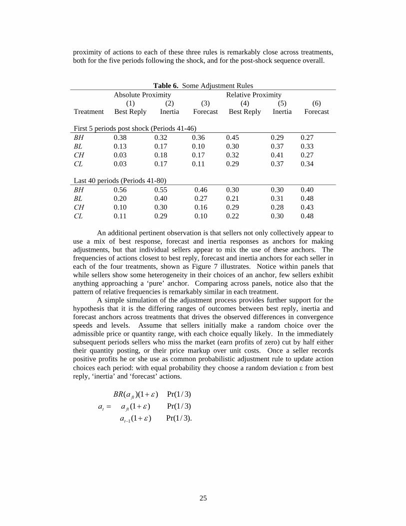
proximity of actions to each of these three rules is remarkably close across treatments, both for the five periods following the shock, and for the post-shock sequence overall.

Table 6. Some Adjustment Rules Absolute Proximity Relative Proximity

Treatment (1)

Best Reply (2)

Inertia (3)

Forecast (4)

Best Reply (5)

Inertia (6)

Forecast First 5 periods post shock (Periods 41-46) BH 0.38 0.32 0.36 0.45 0.29 0.27 BL 0.13 0.17 0.10 0.30 0.37 0.33 CH 0.03 0.18 0.17 0.32 0.41 0.27 CL 0.03 0.17 0.11 0.29 0.37 0.34 Last 40 periods (Periods 41-80) BH 0.56 0.55 0.46 0.30 0.30 0.40 BL 0.20 0.40 0.27 0.21 0.31 0.48 CH 0.10 0.30 0.16 0.29 0.28 0.43 CL 0.11 0.29 0.10 0.22 0.30 0.48

An additional pertinent observation is that sellers not only collectively appear to

use a mix of best response, forecast and inertia responses as anchors for making adjustments, but that individual sellers appear to mix the use of these anchors. The frequencies of actions closest to best reply, forecast and inertia anchors for each seller in each of the four treatments, shown as Figure 7 illustrates. Notice within panels that while sellers show some heterogeneity in their choices of an anchor, few sellers exhibit anything approaching a ‘pure’ anchor. Comparing across panels, notice also that the pattern of relative frequencies is remarkably similar in each treatment.

A simple simulation of the adjustment process provides further support for the hypothesis that it is the differing ranges of outcomes between best reply, inertia and forecast anchors across treatments that drives the observed differences in convergence speeds and levels. Assume that sellers initially make a random choice over the admissible price or quantity range, with each choice equally likely. In the immediately subsequent periods sellers who miss the market (earn profits of zero) cut by half either their quantity posting, or their price markup over unit costs. Once a seller records positive profits he or she use as common probabilistic adjustment rule to update action choices each period: with equal probability they choose a random deviation ε from best reply, ‘inertia’ and ‘forecast’ actions.

).3/1Pr()3/1Pr()3/1Pr(

)1()1(

)1)((

1 εεε

+++

=

−t

ft

ft

t

aa

aBRa

25

CL

0%

20%

40%

60%

80%

100%

Participants

Incidence

CH

0%

20%

40%

60%

80%

100%

ParticipantsBest Reply Deviation Forecast Deviation Inertia Deviation

Incidence

BL

0%

20%

40%

60%

80%

100%

Participants

Incidence

BH

0%

20%

40%

60%

80%

100%

ParticipantsBest Reply Deviation Forecast Deviation Inertia Deviation

v

Incidence

Figure 7. Frequency of Minimum Deviations from Best Reply, Forecast and Inertia (Periods 41-80). At the time of the shock, sellers continue to use this same rule to adjust from the final period of the pre-shock regime, but with the exception that immediately following the shock sellers cut price markups or quantity postings by half each period they miss the market, as they did at the outset.23 The upper and middle panels of Figure 8 illustrate for each treatment, the mean of n= 5000 simulations under the above update rule, with ε∼ U{-.15,.15},and absolute deviations of mean transactions prices from the static Nash equilibrium |)(| NEPP − for each treatment, smoothed with a five period average process to facilitate comparison. Observed results are considerably more volatile than simulated results. Further, observed adjustment speeds in the BH markets are considerably faster than is consistent with the simulations. Nevertheless results of this simple simulation do parallel observed results in the senses that (a) some non-trivial and persistent deviations of prices from static Nash predictions characterize all treatments, and (b) absolute deviations for the BH treatment are considerably smaller than for the other treatments. Further, much of the deviations between simulated and observed BL, CL and CH outcomes may be attributable to tacit collusion or (in the case of session CL-vi) confusion. The bottom panel of Figure 8 illustrates observed absolute mean price deviations after removing the five (of 48) 40-period sequences with cooperation index values φ > 0.20,24 as well as the second sequence of session CL-vi, where persistently large quantity choices by a single confused seller precluded any market adjustment. Given these adjustments, simulation results rank order outcomes quite well.

23 This initial ‘find the market’ rule improves slightly convergence speeds in the BH treatment. As is evident from Figure 8, convergence speeds for BH sellers are considerably higher still than simulated results. Importantly, however, variations in the initial adjustment rule to not affect ultimate convergence levels. Also, for all treatments, simulated mean price deviations equal zero. 24 These are the sessions bolded in Table 4.

26

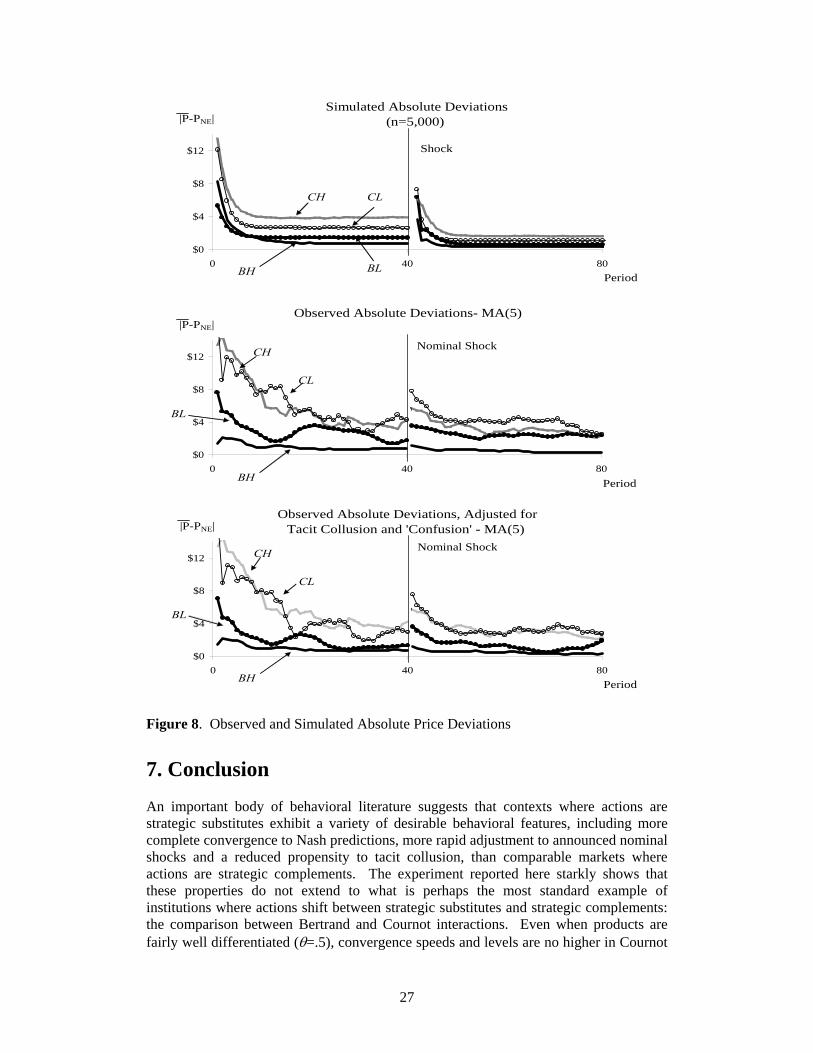
$0

$4

$8

$12

0 40 80BH

BL

CH

CL

v

|P-PNE|

Period

Nominal Shock

Observed Absolute Deviations- MA(5)

$0

$4

$8

$12

0 40 80BH

BL

CH

CL

v

|P-PNE|

Period

Nominal Shock

Observed Absolute Deviations, Adjusted for Tacit Collusion and 'Confusion' - MA(5)

$0

$4

$8

$12

0 40 80BH BL

CH CL

|P-PNE|

Period

Shock

Simulated Absolute Deviations(n=5,000)

Figure 8. Observed and Simulated Absolute Price Deviations 7. Conclusion

An important body of behavioral literature suggests that contexts where actions are strategic substitutes exhibit a variety of desirable behavioral features, including more complete convergence to Nash predictions, more rapid adjustment to announced nominal shocks and a reduced propensity to tacit collusion, than comparable markets where actions are strategic complements. The experiment reported here starkly shows that these properties do not extend to what is perhaps the most standard example of institutions where actions shift between strategic substitutes and strategic complements: the comparison between Bertrand and Cournot interactions. Even when products are fairly well differentiated (θ=.5), convergence speeds and levels are no higher in Cournot

27

markets than in Bertrand markets. If anything, in this case the opposite is true. We do find, however, that Bertrand sellers tend to signal more frequently than Cournot sellers, and when θ=.5, the type of signals sellers send (‘surges’) tends to raise prices in some markets.

As products become closer substitutes the relative superiority of Bertrand markets becomes more clearly evident. When θ=.9 convergence levels and speeds in Bertrand markets substantially and significantly exceed those in their Cournot counterparts. Further, even though Bertrand sellers still attempt to signal intentions to tacitly collude more frequently than their Cournot counterparts when θ=.9, the high costs of sending repeated signals forces sellers to send ‘spikes’ which have little effect on prices.

Our analysis of individual decisions suggests that the observed differences in convergence levels and speeds is driven by a different type of rationality limitation than is discussed in strategic substitutes/strategic complements literature. Rather than differing in their capacities to update expectations, sellers in our markets appear to bounded rationality in the sense that they use forecast and inertia ‘anchors as a basis for action choices in addition to best replies. Given these propensities, Bertrand markets converge more rapidly and more completely to static Nash predictions, particularly when products are close substitutes, because the differences between the various anchors is smaller in Bertrand markets.

These results are important for two related reasons. First, narrowly, we observe that economists should be extremely cautious about applying results regarding the performance of markets with strategic substitutes and complements to the comparison of Cournot and Bertrand institutions. In distinction to the implications of the behavioral literature on strategic substitutes and strategic complements, the results presented here raise very considerable questions about the extent to which Cournot markets may be a preferred form of market organization, or alternatively, the extent to which deciding that a given context is best analyzed as a Bertrand rather than a Cournot context implies that the (Bertrand) market context will exhibit slower or less complete convergence to static Nash predictions.

Second, and more generally, we urge caution in drawing broad inferences about the competitiveness of naturally occurring institutions from very stylized experiments, particularly when results turn on a form of bounded rationality. Experiments that isolate the effects of specific rationality limitations in highly stylized contexts serve an important methodological function of demonstrating that an environment exists where a rationality bound may affect behavior. However, taken alone, such results offer relatively little in the way of insights about the performance of ‘parallel’ natural contexts, since in more complex environments other rationality limitations may also be relevant and the effects of these other limitations may dominate the effects observed in starker, more stylized contexts. To avoid potentially grievous errors, further experimental work, both laboratory research in specific institutional contexts, and, where possible, in the field, is necessary to establish the importance of a particular factor in a given context.

28

References Anderson, Lisa, Beth Freeborn and Charles A. Holt, “Tacit Collusion in Price Setting

Duopoly Markets: Experimental Evidence. Manuscript, College of William and Mary.

Chen Yan and Robert Gazzale (2004) “When Does Learning in Games Generate

Convergence to Nash Equilibria? The Role of Supermodularity in an Experimental Setting” American Economic Review 94, 1505-1535

Davis, Douglas D. (1999) “Advance Production and Cournot Outcomes: An

Experimental Investigation,” Journal of Economic Behavior and Organization 40, 59-79.

Davis, Douglas D. (2002) “Strategic Interactions, Market Information and Mergers in

Differentiated Product Markets: An Experimental Investigation,” International Journal of Industrial Organization 20(9) 1277-1312.

Davis, Douglas D., (2008) “Pure Numbers Effects, Market Power and Tacit Collusion in

Posted Offer Markets” manuscript, Virginia Commonwealth University. Daughety, Andrew F. (2008) “Cournot Competition” The New Palgrave Dictionary of

Economics 2nd Steven N. Durlauf and Lawrence E. Blume, eds. Palgrave Macmillan: New York.

Fehr, Ernst and Jean-Robert Tyran (2008) “Limited Rationality and Strategic

Interaction: The Impact of the Strategic Environment on Nominal Inertia” Econometrica 76 (2), 353–394.

Fisher, Franklin (1961) “The Stability of the Cournot Oligopoly Solution: The Effects of

Speeds of Adjustment and Increasing Marginal Costs,” Review of Economic Studies 29, 125-135.

Haltiwanger, H. and Waldman M. (1985) “Rational Expectations and the Limits of

Rationality: An Analsis of Heterogeneity” American Economic Review, 75(3) 326340

Heemeijer, Peter, Cars Hommes, Jeop Sonnemans and Jan Tuinstra (2007) “Price

Stability and Volatility in Markets with Positive and Negative Expectations Feedback: An Experimental Investigation,” Journal of Economic Dynamics and Control (forthcoming)

Holt, Charles A. (2005) “Industrial Organization: A Survey of Laboratory Research” in

J. Kagel and A. Roth (eds.) Handbook of Experimental Economics, Princeton UP: Princeton.

Huck, Steffen, Hans-Theo Normann and Jörg Oechssler (2002) “Stability of the Cournot

process: Experimental Evidence” International Journal of Game Theory, 2002, Vol. 31, 123-136

29

Huck Steffen, Hans-Theo Normann and Jörg Oechssler (2000) “Does Information about Competitors’ Actions Increase or Decrease Competition in Experimental Oligopoly Markets?” International Journal of Industrial Organization 18, 39-57.

Milgrom, Paul R. and John Roberts (1990) Rationalizibility, Learning and Equilibrium

in Games with Strategic Complementarities,” Econometrica, 58, 1255-77. Offerman, Theo, Jan Potters and Joep Sonnemans (2002) “Imitation and Belief Learning

in an Oligopoly Experiment,” Review of Economic Studies 69, 973-997. Potters, Jan and Sigrid Suetens (2008) “Strategic Interaction, Externalities and

Cooperation: Experimental Evidence.” Review of Economic Studies (forthcoming)

Rassenti, Stephen, Stanley Reynolds, Vernon L. Smith and Ferenc Szidarovszky (2000)

“Adaptation and Convergence in Experimental Cournot Games” Journal of Economic Behavior and Organization, 41 117-146.

Siegel, Sidney and Castellan, N. John Jr. Nonparametric Statistics for the Behavioral

Sciences, 2nd ed. New Yourk: McGraw-Hill, 1988. Suetens, Sigrid and Jan Potters (2007) “Bertrand Colludes More than Cournot?”

Experimental Economics, 10, 71-77. Theocharis, R. D. (1960) “On the Stability of the Cournot Solution to the Oligopoly

Problem,” Review of Economic Studies 27, 133-134. Topkis, Donald (1979) “Equilibrium Points in Nonzero-Sum N-Person Submodular

Games,” SIAM Journal on Control and Optimization, 17 773-787 Vega-Redondo, Fernando (1997) “The Evolution of Walrasian Behavior,” Econometrica

65, 375-84. Vives, Javier (1999) Oligopoly Pricing: Old Ideas and New Tools. Cambridge, MIT

Press.

30

Appendix. Sample Experiment Instructions.

(BH treatment). Overview: This is an experiment in the economics of decision-making. Various research foundations have provided funds for this research. The instructions are simple, and if you follow them carefully and make good decisions, you may earn a considerable amount of money that will be paid to you in CASH at the end of the experiment. Your earnings will be determined partly by your decisions and partly by the decisions of others. General Description. You run a firm that produces and sells a certain product.

1. Besides you there are 3 other firms in your industry producing similar but not identical products.

2. The market consists of 80 periods. Each period lasts up to 90 seconds. A period will also end when the last seller makes his or her decisions for the period. If this is less than 90 seconds, the period will end early.

3. Your primary task in every period is to decide the price of your product 4. Your price decision and average price of the other sellers determine your sales.

The higher your price, the fewer units you sell. (In fact, above a certain price you don’t sell anything). The higher the price of the other sellers, the more units you sell.

5. You earn profits by selling at prices above costs. All firms produce with the same unit cost. Initially this cost is 8 lab dollars per unit.

6. Your price can be no lower than your unit cost (initially 8 lab dollars). You may post any price you like up to a maximum of 50 lab dollars

7. Each period you will also predict the average price choices of the others in your market. If your forecast is within 30¢ of the actual average price, you will earn 1 lab dollar.

8. Trading follows a simple two-step process. First all sellers submit pricing decisions and forecasts. Second, an automated buyer makes purchases.

9. The automated buyer makes purchases according to the following rule. iii ppq −+−= 29.757.762.21

Where ip− is the average of the prices posted by the other three sellers. An equivalent way to express the relationship between price and sales quantities is

iiii qqpp −− −−= 7.280 where iq− is the average of the quantities that that buyer purchases from the

other three sellers. We will use this latter relationship later in the experiment 10. Unit costs and the above purchasing rule will remain in effect for 40 periods. 11. Your laboratory earnings for the first 40 periods will be converted to U.S

currency at a rate of 200 lab dollars = $1 U.S. Specific Instructions. Below is a sample screen for a seller P2 in a four firm industry at the start of period 3. In period 3, seller P2 must enter a price decision in the Price box and a forecast of average price other will post for the period in the Forecast box given the unit costs in the ‘Unit Cost’ box. Seller P2 has 85 seconds left to make his or her choices and to submit them by clicking the Submit button. (Alternatively, you

31

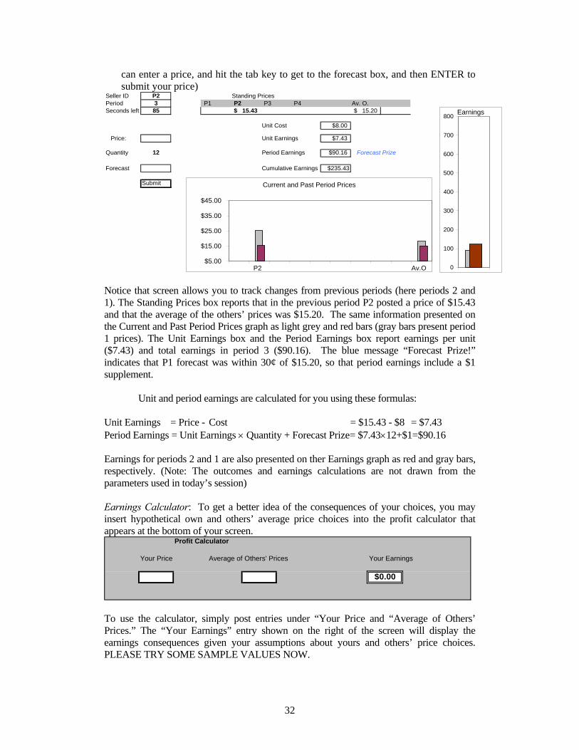
can enter a price, and hit the tab key to get to the forecast box, and then ENTER to submit your price)

Seller ID P2 Standing PricesPeriod 3 P1 P2 P3 P4 Av. O.Seconds left 85 15.43$ 15.20$

Unit Cost $8.00

Price: Unit Earnings $7.43

Quantity 12 Period Earnings $90.16 Forecast Prize

Forecast Cumulative Earnings $235.43

Submit Current and Past Period Prices

$5.00

$15.00

$25.00

$35.00

$45.00

P2 Av.O 0

100

200

300

400

500

600

700

800 Earnings

Notice that screen allows you to track changes from previous periods (here periods 2 and 1). The Standing Prices box reports that in the previous period P2 posted a price of $15.43 and that the average of the others’ prices was $15.20. The same information presented on the Current and Past Period Prices graph as light grey and red bars (gray bars present period 1 prices). The Unit Earnings box and the Period Earnings box report earnings per unit ($7.43) and total earnings in period 3 ($90.16). The blue message “Forecast Prize!” indicates that P1 forecast was within 30¢ of $15.20, so that period earnings include a $1 supplement.

Unit and period earnings are calculated for you using these formulas:

Unit Earnings = Price - Cost = $15.43 - $8 = $7.43 Period Earnings = Unit Earnings × Quantity + Forecast Prize= $7.43×12+$1=$90.16 Earnings for periods 2 and 1 are also presented on ther Earnings graph as red and gray bars, respectively. (Note: The outcomes and earnings calculations are not drawn from the parameters used in today’s session) Earnings Calculator: To get a better idea of the consequences of your choices, you may insert hypothetical own and others’ average price choices into the profit calculator that appears at the bottom of your screen.

Profit Calculator

Your Price Average of Others' Prices Your Earnings

$0.00

To use the calculator, simply post entries under “Your Price and “Average of Others’ Prices.” The “Your Earnings” entry shown on the right of the screen will display the earnings consequences given your assumptions about yours and others’ price choices. PLEASE TRY SOME SAMPLE VALUES NOW.

32

You may use the earnings calculator as much or as little as you wish.

Period 41 Instructions (Handed out after period 40 and read aloud)

Conditions for the next 40 periods will be identical to those for the initial 40 periods, with the following 3 differences 1. Unit costs will fall from $8 per unit to $4 per unit 2. The purchasing rule used by the buyer will be

iii ppq −+−= 29.757.781.10 Where ip− is the average of the prices posted by the other three sellers. An equivalent way to express the relationship between price and sales quantities is

iii qqp −−−= 7.240 Notice from this alternative expression that the demand intercept falls from 80 to 40 3. The conversion rate of lab dollars to U.S. Currency will change increase from $200 lab = $1 U.S. to 50 lab dollars = $1 U.S.

4. In words, each lab dollar is now worth four times more than in the first portion of the experiment. If for example, if you earned $100 lab dollars in period 40, your earnings in U.S. currency would have been 100/200 = 50¢. If you earn 100 lab dollars in period 41, your earnings would be 100/50 = $2.

33