Embed Size (px)
Citation preview

NBER WORKING PAPER SERIES
DO TAXPAYERS BUNCHAT KINK POINTS?
Emmanuel Saez
Working Paper 7366http://www.nber.org/papers/w7366
NATIONAL BUREAU OF ECONOMIC RESEARCH1050 Massachusetts Avenue
Cambridge, MA 02138September 1999
I am very grateful to Dan Feenberg for his help with the tax returns data. I thank Peter Diamond, EstherDuflo, Jon Gruber, Roger Guesnerie, James Poterba and Todd Sinai for helpful comments and discussions.Financial support from the Alfred P. Sloan Foundation is thankfully acknowledged. The views expressedherein are those of the authors and not necessarily those of the National Bureau of Economic Research.
© 1999 by Emmanuel Saez. All rights reserved. Short sections of text, not to exceed two paragraphs, may

be quoted without explicit permission provided that full credit, including © notice, is given to the source.Do Taxpayers Bunch at Kink Points?Emmanuel SaezNBER Working Paper No. 7366September 1999JEL No. H31
ABSTRACT
This paper investigates whether taxpayers bunch at the kink points of the US income tax schedule
(i.e. where marginal rates jump) using tax returns data. Clear evidence of bunching is found only at the first
kink point (where marginal rates jump from 0 to 15%). Evidence for other kink points is weak or null.
Evidence of bunching is stronger for itemizers than for non-itemizers. Theoretical models of behavioral
responses to taxation show that bunching is proportional to the compensated elasticity of income with
respect to tax rates. These models are used to perform simulations of bunching and calibrate the key
parameters (the behavioral elasticity and the extent to which taxpayers control their income) to the empirical
income distributions. Except for low income earners, the behavioral elasticity consistent with the empirical
results is small.
Emmanuel Saez Harvard UniversityDepartment of EconomicsLittauerCambridge, MA 02138and [email protected]

1 Introduction
Most empirical studies about labor supply and the behavioral responses to income taxation
use the classical static micro-economic model where agents choose to supply e�ort until
the marginal disutility becomes equal to marginal bene�ts. This usual model predicts
that if indi�erence curves are well behaved and preferences are smoothly distributed, we
should observe bunching at convex kink points of the budget set. Taxes and government
transfers are a good example of institutions introducing kink points in budget sets. For
example, the federal income tax imposes a piecewise-linear schedule by the use of constant
marginal rates between brackets. The payroll tax in the Social Security system likewise
generates a (concave) kinked schedule because the marginal rate drops to zero above a
certain earnings maximum. Many government transfer programs also introduce piecewise-
linear constraints because transfer bene�ts are progressively \taxed" away as income rises
until the point where an individual or household loses eligibility for the bene�t altogether.
A strand of the empirical labor supply literature has explicitly taken into account the
predictions of economic theory in the case of kinky budget constraints in order to improve
estimation of labor supply behavior. This method, known as the non-linear budget set
estimation method, reckons explicitly that maximizing utility agents must be either on a
linear part of the budget set or at a convex kink point. This method was �rst developed by
Burtless and Hausman (1978) to study the Negative Income Tax experiments. Hausman
(1981) then applied this method for the �rst time to study the e�ect of the federal income
tax on labor supply. Afterwards, this method has been applied to many government
transfer programs. Mo�t (1990) provides a non-technical presentation of the non-linear
budget set method and a survey of applications. However, the bunching issue has not
attracted much interest even in this type of studies because, in most cases, a casual look
at the data does not reveal evidence of bunching at the kink points. Heckman (1982)
early criticized Hausman's studies of the e�ect of the income tax on labor supply arguing
that no evidence of bunching could be found in the data. As Hausman (1982) replied
however, this does not necessarily invalidate that approach because measurement error is
2
present in the data and is modeled by adding an error term to the labor supply equation.
As a result, there are few studies that document the evidence of bunching of agents
at the kink points generated by taxes or transfer programs. Burtless and Mo�t (1984)
and Friedberg (1998) observed bunching behavior in the case of elderly who receive social
security bene�ts but are still working. Social security bene�ts are taxed away when
earned income exceeds an exemption amount. Tax rates vary from 33% to 50% and thus
generate big kinks in the budget set of the elderly. Liebman (1998) looked at the income
distribution of Earned Income Tax Credit recipients but found no evidence of bunching
at the kink points generated by this program. No study has carefully examined the
evidence of bunching at the kink points of the income tax schedule. This is striking for
two reasons. First, such a study could give an indirect proof of the existence of behavioral
responses to taxation which is the object of a very controversial debate in the public
economics literature. Second, studying bunching is relatively straightforward and only
requires micro-economic data on taxable income.
The �rst goal of the present paper is thus to investigate whether there is evidence of
bunching at the kink points of the US income tax from 1979 to 1994. This study uses
the large cross-sections of tax returns provided annually by the Internal Revenue Service.
This data is perfectly suited because it gives information about the precise location of
taxpayers on the tax schedule.1
Theoretically, the size of bunching around kink points depends critically on the com-
pensated elasticity of income with respect to marginal taxes. Unsurprisingly, high elastic-
ities should lead to high levels of clustering. The compensated elasticity is one of the key
parameters to devise an optimal income tax policy. However, estimates vary considerably
from very low estimates in the classical labor supply literature (see Pencavel (1986) for
a survey) to very high estimates in recent literature looking directly at taxable income
1The most widely used datasets such as the PSID or the CPS do not provide the precise location
of taxpayers on the tax schedule because all sources of income or deductions are not reported precisely
enough. This may partly explain why the issue of bunching has remained under-investigated for so long.
3

(see Lindsey (1987) and Feldstein (1995)). Therefore, it is potentially very interesting to
try to estimate this elasticity using the size of bunching. These indirect estimates, as in
Lindsey's and Feldstein's studies, are based directly on taxable income and thus could
provide additional evidence on this controversial issue in public economics.
Of course, perfect bunching at the kink points of the tax schedule is not observed in the
data because taxpayers cannot perfectly �ne-tune their labor supply nor control perfectly
all their sources of income. Therefore, the second part of this paper develops theoretical
models to try to understand how this uncertainty element a�ects bunching. If taxpayers
can control their incomes only imperfectly, a kink in the tax schedule should generate a
hump in the income distribution. The better taxpayers control their incomes, the closer
the hump is clustered around the kink point. It is di�cult, using micro longitudinal data
on income, to estimate to what extent agents can control their incomes because it is not
possible to distinguish variations in income due to a voluntary choice from those due
to random and uncontrolled factors. This issue is especially important in consumption
theory where it is very important to tell apart transitory (random) income shocks from
voluntary income changes (see e.g. Deaton (1992), Chapter 3). Sharp clustering around
the kink points would be evidence that the random factor is small whereas at clustering
would suggest that random factors are important. Thus, the study of bunching is also
interesting because it provides an indirect way to measure to what extent taxpayers can
control the process generating their incomes.
The remaining of the paper is organized as follows. Section 2 presents the data and
the tax schedules of the period 1979 to 1994. Section 3 displays the empirical results.
The distributions of taxable income are estimated using non parametric kernel density
methods. Section 4 presents a simple theoretical model to investigate how the size of
bunching is related to the elasticity and the extent to which taxpayers control their income.
Section 5 presents simulations of income distributions using this theoretical model. I
calibrate the key parameters that reproduce the evidence of bunching found in empirical
distributions. Section 6 provides a brief conclusion and discusses methodological and
4

policy implications.
2 Data and Tax Schedules
According to the usual micro-economic model, taxpayers increase their income until the
marginal utility of the last dollar earned less the marginal tax rate paid on this last dollar
is equal to the marginal cost that is spent to earn this last dollar. Therefore, the key
parameter in the income equation is one minus the marginal tax rate which I call the
net-of-tax rate. Thus a given kink point produced by a jump in marginal rates from
t1 to t2 (t1 < t2) generates high levels of bunching if the ratio the two net-of-tax rates
(1 � t2)=(1 � t1) is signi�cantly smaller than one. In another words, a jump from 0 to
10% in marginal rates should have the same e�ect than a jump from 90% to 91%. From
now on, I call this key ratio the net-of-tax ratio.
I use tax returns data constructed by the Internal Revenue Service (IRS), and known
as the Individual Public Use Tax File, to carry out this study. The data are annual cross-
sections available from 1960 to 1994 but I focus only on years 1979 to 1994 because before
1979, the number of brackets in the tax schedule was very large and thus the size of the
jumps was small. The average number of observations per year is slightly above 100,000.
The annual cross sections are strati�ed random samples with high sampling rates for
wealthy taxpayers. Taxpayers pay taxes on taxable income which is equal to total income
less personal exemptions and other additional deductions. Taxes are computed directly
from a piece-wise linear tax schedule as a function of taxable income. Therefore, taxable
income is the relevant variable for the present study. Tax schedules di�er according to
marital status which can be either Married, Single or Head of household. As more than
90% of returns are �lled by Married or Single taxpayers, I restrict my study to these two
marital status only.
I now review the main characteristics and changes in the US tax schedule from 1979
to 1994.
5
From 1979 to 1981, the number of brackets was fairly high (around 14). The rates
went as high as 70% but the part of capital gains subject to tax was limited to 40% and
the maximum tax rate on earned income was equal to 50%. The size of the jumps in the
tax schedule was around 4-7% (see Table I). There was one big jump at the �rst kink
point where marginal rates jumped from 0 to 14% at a very low level of income. The
tax schedule was not indexed for in ation. In ation was high (around 10%) from 1979 to
1981 and thus this increased substantially the burden of the income tax.
In 1981, the Economic Recovery Tax Act (ERTA) decreased marginal rates in three
years from 1982 to 1984. The top-rate was reduced to 50% and the tax brackets were
extended. The location of kink points did not change, but the corresponding marginal
rates were decreased (see Table II). Moreover, from 1984 on, the tax schedule became
indexed to in ation. In 1986, the Tax Reform Act (TRA) introduced the largest changes
in the income tax since World War II. The number of brackets was drastically reduced
and the top-rate was further reduced to 28%. There were basically two jumps in marginal
rates left: a �rst jump from 0 to 15% and a second jump from 15 to 28%. The TRA
also extended the tax base in order to be a broadly revenue neutral tax reform. The
former exclusion of 60% of capital gains was suppressed. In 1990, an additional bracket
was included, increasing the top rate from 28% to 31%. However, the top rate on capital
gains was left unchanged at 28%. Last, in 1993, the OmniBus Reconciliation Act (OBRA)
added two more brackets at high incomes: one bracket with a marginal rate of 36% and
a top-bracket with marginal rate of 39.6% (see Table II).2
Tax schedules for married taxpayers and singles for years 1979, 1984 and 1994 are
displayed in Tables I and II. I report the location of the jumps in marginal rates in
current dollars on column (1) for Married taxpayers and in column (4) for Singles. In
column (2) for Married taxpayers and column (5) for Singles, I present the marginal rates
corresponding to the jump. Last, in column (3) (for Married taxpayers) and column (6)
(for Singles), I report the corresponding net-of-tax ratios (i.e. the values (1� t2)=(1� t1)).
2The top-rate on capital gains was also left unchanged at 28%.
6
From 1979 to 1994, there has always been a big jump at the end of the �rst bracket:
from 0 to about 11-15% (depending on the years). This kink point is particular because
not only does the marginal rate jump but also because people do not owe any taxes if
they do not reach that income level. From now on, I will call this kink point the �rst kink
point.
I divide the data into two periods. One period for years before the TRA of 1986 (years
1979 to 1986). In that period, there were many kink points besides the �rst kink point.
The second period is for years after the TRA (years 1988 to 1994). In that later period,
there were essentially two kink points: the �rst kink point and an additional jump from
15 to 28%. Year 1987 is excluded because it is a transition year.3
3 Empirical Results
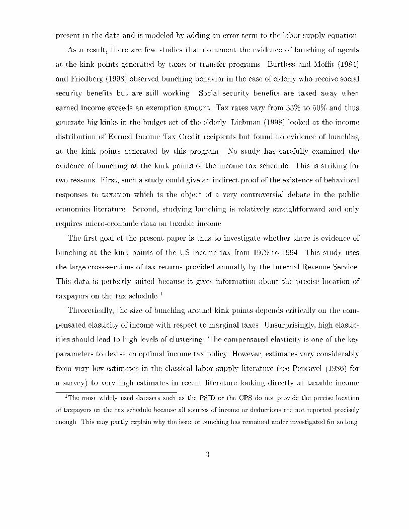
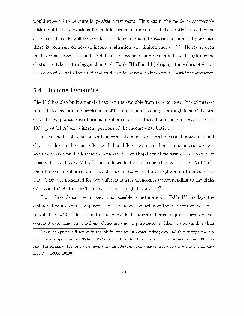
I �rst test whether there are atoms of taxpayers at the kink points of the tax schedule.
This would be case as soon as a non negligible set of taxpayers could control nearly
perfectly their incomes4 (I come back in more detail to this point in Section 4). The best
way to check this hypothesis is to draw a histogram of the income distribution with small
bandwidth. If there were an atom (even if small) at a given kink point then this should
appear on the histogram when the size of the bandwidth decreases. As evidenced on
Figure 3.1 for years 1979 to 1981, looking at the kink points does not reveal such atoms.
The loci of the kink points are represented by vertical dashed lines. Other years or
other portions of the income distribution would not reveal anymore evidence of bunching.
Therefore, we can reject the hypothesis of the existence of a non-negligible number of
taxpayers controlling perfectly their taxable income.
If we assume that taxpayers do not control perfectly their income then they will not be
3The tax changes of the TRA were not fully phased in until 1988. The number of brackets in 1987
was intermediate between the pre TRA and post TRA periods.4Note that taxpayers should control not only their incomes but also their possibly numerous deductions
and adjustments that are subtracted from gross income to compute taxable income.
7

able to bunch perfectly at the kink points but will tend to cluster around these points. The
better taxpayers control their incomes, the sharper the humps. As I now look for humps
in the distribution that could be generated by kink points, it is no longer appropriate
to rely on histograms. Thus, income densities will be estimated using the kernel density
method which is described in appendix. All kernel estimates are plotted along with 95%
point-wise con�dence intervals.
Results are presented in Figures 3.2 to 3.17. Year, marital status, number of obser-
vations and the bandwidth used in the density estimation are reported in the title. The
dashed vertical lines represent the kink points. The jump in tax rates and the level of
taxable income corresponding to the kink points are reported on the Figures.5
3.1 Low and middle incomes
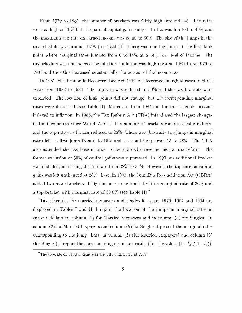
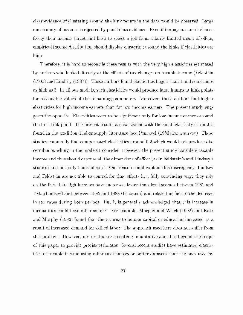
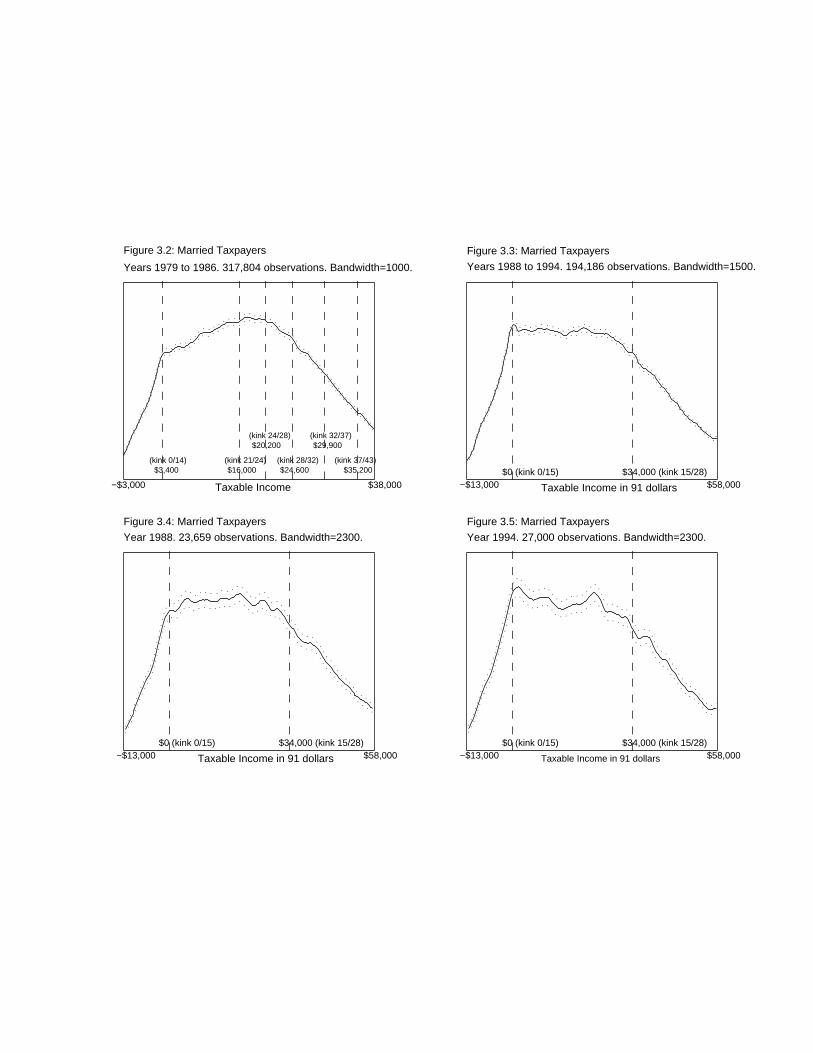
Estimates for married taxpayers are given on Figures 3.2 to 3.5. The density estimate for
years6 before the TRA is reported on Figure 3.2 and on Figure 3.3 for years after TRA.7
The �rst striking point to notice is that income distributions display an irregularity
around the �rst kink point. The distributions present a clear kink around that income
level. The TRA shifted the location of the �rst kink point to the right because the
standard deduction and the personal exemptions were increased.8 I can test whether
taxpayers adapted slowly or not to these changes by comparing year 1988 (�rst year in
which the tax reforms of the TRA were fully phased in) and year 1994 (the most recent
year available). The estimates are reported on Figures 3.4 and 3.5. The results show
clearly that bunching is much more important in 1994 than in 1988. The deformation of
5Before the TRA of 1986, there are in fact more kink points than represented because I omit to
represent kinks corresponding to jumps smaller than 3 percentage points.
6I explain in appendix the procedure I use to produce income densities merged over several years.7Note that the location of the �rst kink point shifts to 0 after the TRA. This is due to the change in
the de�nition of taxable income. The standard deduction is no longer included in taxable income after
TRA.
8The TRA reduced signi�cantly the number of households liable for the federal income tax.
8

the income distribution is much more important in 1994 than in 1988. Therefore, this
con�rms the presumption that taxpayers cannot adapt immediately their behavior to the
tax schedule.
The second striking fact is the absence of any clear humps around the other kink points.
This could be understandable before the TRA because the other jumps are not very big
and the tax rates not high at those incomes (implying that the net-of-taxes ratios are close
to one as shown in Tables I and II). However, more surprisingly, nothing is distinguishable
around the second kink point (jump 15/28) after the TRA86. Moreover, there is no more
evidence of bunching in 1994 than in 1988 (see Figures 3.4 and 3.5). Therefore even in
1994, i.e. seven years after the TRA was implemented, taxpayers do not cluster around
the second kink point. This implies that either low income and middle income earners do
not behave in the same way or that the �rst kink point is perceived di�erently from the
other kink points. At this early stage, we can presume that either middle income earners
control less accurately their income or that their elasticity with respect to marginal rates
is lower. The argument will be made more precise in the following sections.
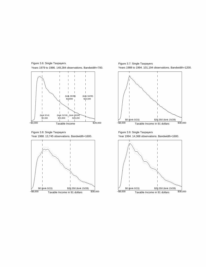
The same estimates for singles are reported on Figures 3.6 to 3.9.9 The general shape
of the income distribution of single taxpayers is di�erent from the distribution of married
taxpayers because the mode of the distribution is sharper and the top tail is thinner. In
fact the mode was lower than the �rst kink point before the TRA86 and then became
almost centered on the �rst kink point after 1986. Before 1986, the distribution density is
quickly decreasing around the �rst kink point making the hump around that kink point
less discernible everything else being equal. We can nevertheless see a small hump around
the �rst kink point on Figure 3.6. After 1986 (Figure 3.7), the �rst kink corresponds
exactly to the mode of the distribution and thus it is hard to tell apart what is really due
9I have excluded from the data taxpayers claimed as dependents because special rules apply for them
and this tends to create arti�cial bunching around the �rst kink point. Dependent taxpayers have a
smaller standard deduction but can deduct earned income up to a certain amount. As a result, many of
them have taxable income arti�cially close to 0.
9

to bunching behavior. Figures 3.8 and 3.9 (for years 1988 and 1994) give an interesting
insight about the dynamics of bunching. The mode is on the right of the kink point on
Figure 3.8 and there is no clear evidence of bunching for year 1988. Figure 3.9 is completely
di�erent: the mode is centered exactly on the kink point and is sharper. Estimates for
each year between 1988 and 1994 would show a progressive pattern toward more and
more bunching. Thus, it is plausible to think that the deformation of the distribution
around the mode between 1988 and 1994 is due to taxpayers' responses to marginal rates.
Bunching is increasing over time as taxpayers adapt slowly their behavior to the new tax
schedule. The evidence concerning the second kink after the TRA of 1986 reveals no more
bunching than for married taxpayers. Once again, there is no more evidence of bunching
in 1994 than in 1988.
A technical objection about the special result for the �rst kink point could be raised.
There is a threshold gross income level under which people are not required to �ll a return.
This threshold varies with the marital status and is equal to the basic personal exemptions
(two for married taxpayers and one for singles) plus the standard deduction.10 As a result,
it may be possible that the shape of the distribution is arti�cially kinky around the �rst
kink point because non-�lers are missing on the left of the kink point. Fortunately, the
fact that, in the US tax-system, a large part of taxes are withheld allows to test whether
this objection is relevant. When somebody expects a refund from the IRS, he has to
�ll a return to get it. Therefore, people expecting a refund have good incentives to �ll.
Moreover, withholding is rarely perfect and thus most taxpayers either expect a refund
or have to pay an additional amount to the IRS. 11 Therefore there should be no arti�cial
irregularity around the �rst kink point for people expecting a refund. Around the �rst
10The threshold does not take into account additional personal exemptions for dependents. For exam-
ple, a married household claiming children exemptions may be required to �ll even if its income is less
than the sum of all its exemptions plus the standard deduction.11As evidenced from Figure 3.6, before TRA, the mode of the income distribution for singles is on
the left of the �rst kink point, implying that many low income people �ll tax returns in order to obtain
refunds though they their �nal tax liability is zero.
10

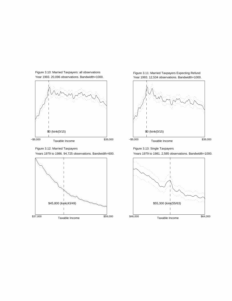
kink point, the distributions of taxable income for people expecting a refund are almost
the same as the full distributions. This is displayed on Figures 3.10 and 3.11. Figure 3.10
represents the full distribution of incomes for year 1993 and Figure 3.11 represents the
distribution of incomes for taxpayers expecting a refund. This similarity is due to the
fact that a vast majority of low income earners expect a return from the IRS. Evidence of
bunching is not reduced for people expecting a refund; therefore the irregularity around
the �rst kink point is not due to missing taxpayers.
An alternative way of testing this objection is to estimate the density of gross incomes
and check whether there is an irregularity around the threshold level of �ling requirement.
These estimations do not reveal anything irregular con�rming the fact that low incomes
�ll returns to get refunds even though they are not legally required to do so.
3.2 High income earners
Before TRA86, the tax schedule had a much more progressive structure with many
kink points at the high end of the income distribution which could generate bunching
behavior.12 Nevertheless, I could �nd no humps at any other kink points for married
taxpayers for years 1979 to 1986. Humps around kink points are either absent or not
robust across years. Estimates aggregated over several years do not show bunching. An
estimation for the kink 43/49 at income level 45,800 dollars for years 1979 to 1986 is pre-
sented on Figure 3.12.13 It does not show any evidence of bunching, though the number
of observations is very large (nearly 100; 000). The tax schedule for singles for years 1979
to 1981 presented a very big jump from 55 to 63%. The estimate obtained merging the
three years reveals slight evidence of bunching: there is a small hump around the kink
point (see Figure 3.13). This is the only high bracket kink point that presented some
12Note also that two new kink points were introduced in 1993: from 31 to 36% and from 36 to 39.6%.
These kinks did not reveal bunching in 1993 or 1994. This can obviously be explained by the fact that
taxpayers take time to adapt their behavior.13In fact, the jump was 43/49 only for years 1979 to 1981. After 1981, there remained a kink exactly
at that income level but the marginal rates changed (the new jump was 33/38).
11

evidence of bunching.
Three facts can partly explain these negative results. First, before the TRA86, tax-
payers could use the average income schedule to reduce their tax liabilities if they had
experienced a substantial increase in taxable income. The tax schedule depended then
not only on current income but also on taxable income in previous years and therefore
the location of kinks varied across taxpayers. The proportion of taxpayers using the av-
erage income schedule becomes higher and higher as taxable income increases. Second,
before 1982, the rule of the 50% percent maximum tax on earned income creates an ad-
ditional problem. Taxpayers claiming earned income followed a di�erent tax rule when
their income reached the level at which they would normally have faced marginal rates
above 50%. This may a�ect bunching for the highest kinks. Discarding, however, those
taxpayers did not reveal clearer evidence of bunching. Last, the tax schedule was �xed in
nominal terms for years 1979 to 1981 while in ation was still high (around 10%). There-
fore, the location of the kinks changed in real terms year after year and so it may have
been more di�cult for taxpayers to adapt to the kinks.
3.3 Itemizers versus non-itemizers
Not all sources of income are controlled to the same extent. As the dataset describes
precisely all the di�erent sources of income, it is possible to study whether taxpayers
bunch more or less according to the type of income they receive. In particular, the types
of incomes which are underreported are likely to reveal more bunching because taxpayers
may underreport part of these incomes in order to avoid entering high brackets. Itemized
deductions are likely to be overstated for the same reasons. Capital gains may or may
not also be realized in order to avoid paying high marginal taxes. I explore various cases
in this subsection.
Self employment income is a source of income commonly underreported. However,
looking at taxpayers reporting self employment income around the second kink point
after the TRA does not reveal any more bunching (I do not reproduce the estimates).
12

Similarly, no evidence of bunching could be found around the second kink point for tax-
payers reporting capital gains after the TRA.
As explained above, in the US income tax system, taxpayers can either choose a
standard deduction of a given amount (depending on marital status) or choose to itemize
deductions (such as medical expenses or work related expenses) if these deductions exceed
the standard deduction. Dividing taxpayers between itemizers and non-itemizers reveals
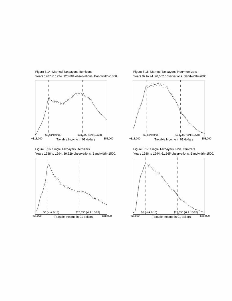
more interesting patterns. The estimates are plotted on Figures 3.13 and 3.14 for married
taxpayers and on Figures 3.15 and 3.16 for singles. I have reproduced only the estimates
for years after TRA. The estimates for itemizers are represented on the left panels and
those for non-itemizers on the right panels. For married taxpayers, the distribution for
itemizers is very di�erent from the general one because most low income earners do not
itemize. Therefore the mode for itemizers is located farther on the right. There is a clear
hump around the �rst kink point for itemizers. The picture for single taxpayers is even
more striking. The peak at the kink point on Figure 3.15 is very large whereas the peak
Figure 3.16 is much smoother than the peak for the whole sample (compare with Figure
3.7). Estimates are also interesting around the second kink point. For non-itemizers
there is no bunching at all. However, the distribution for married itemizers reveals some
bunching.14
It is possible to extend this kind of study to most sources of income such as interest
income, dividends, business income, pensions. However, looking at distributions for tax-
payers reporting these particular types of income did not reveal more evidence of bunching
than the full distribution.
4 Theoretical Models
The aim of this Section is to construct a simple theoretical model of taxation to understand
the phenomenon of bunching. I will particularly examine how the quantity of bunching
14The evidence is much less clear around the second kink for singles.
13

depends on relevant parameters of the model. This model will later allow us to simulate
income distributions in order to compare them with real empirical distributions. I present
a very simple model of taxation similar to the model of optimal taxation of Mirrlees (1971).
4.1 Certainty case
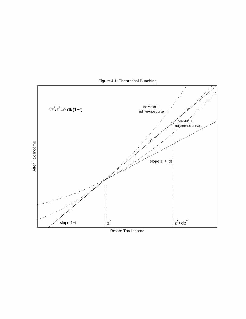
Assume that there is a kink in budget set at income level z� and that marginal tax rates
jumps from t to t + dt at z� as displayed on Figure 4.1. We would like to construct a
measure of bunching at z� to assess how many taxpayers bunch at z� as a function of
dt and the characteristics of the taxpayers. As displayed on Figure 4.1, all taxpayers,
whose indi�erence curve crossing the point (z�; z��T (z�)) remains above the budget set,
bunch at the kink. The indi�erence curve of the the lowest ability individual (denoted
individual L) who bunches at the kink is tangent to the budget set segment on the left of
the kink (slope 1�t). The indi�erence curve of the the highest ability individual (denoted
individual H) who bunches at the kink is tangent to the budget set segment on the right
of the kink (slope 1� t� dt).
In the absence of kink, the budget set would have a constant slope 1� t. In that case,
individual L would still choose income level z�. Individual H, however, would have a tax
rate reduced by dt, and thus would choose a income level z� + dz� such that,
dz�
z�= e
dt
1� t(1)
where e represents the compensated elasticity of income with respect to marginal tax
rates. When the kink is introduced, all taxpayers whose incomes are between z� and
z� + dz� in the no kink case, start bunching at the kink z�. Thus the total number of
taxpayers bunching at z� is simply h(z�)dz� where h(z�) is the density of incomes at z�
when there is no kink point and dz� is given by equation (1). This derivation shows
that bunching is proportional to the compensated elasticity e and to the net-of-tax ratio
dt=(1� t).15
15In the case of large jumps (high dt=(1 � t)), income e�ects should be introduced, the elasticity e
14

Let us consider a simple analytical example to illustrate previous calculations. As in
Mirrlees (1971), I assume that all taxpayers share the same utility function U(c; l) where c
represent after-tax income available for consumption and l represents e�ort. I assume that
U represents convex preferences and is increasing in c and decreasing in l. Each taxpayer
is characterized by a skill (or wage rate) n. When a taxpayer with skill n chooses e�ort l,
he gets income z = nl. The skill parameter n is distributed in the population according
to the density function g(n). I note T (z) the real tax schedule. Consider the following
utility function,
U(c; l) = c�lk+1
k + 1(2)
The elasticity of income with respect to one minus the marginal tax rate (denoted by e)
is constant and equal to 1=k. In this simple case, there are no income e�ects and thus,
compensated and uncompensated elasticities are the same. Assume that z� is an income
level at which marginal rates jump from t1 to t2, (t1 < t2 and thus dt = t2 � t1) then all
taxpayers whose skill lies in [n1; n2] will bunch at z�, where n1 and n2 are de�ned such
that:16
n1(1� t1) = (z�=n1)k (3)
n2(1� t2) = (z�=n2)k (4)
Taking the ratio of these two equations, we obtain,
n2
n1
=
�1� t1
1� t2
� 1
k+1
(5)
would no longer be a pure compensated elasticity but a mix of compensated elasticity and uncompensated
elasticity. However, as long as dt=(1� t) is relatively small, which is always the case with the empirical
kinks considered in Section 3, these income e�ects can be safely neglected.16The individual with skill n1 is individual L and the individual with skill n2 is individual H of Figure
4.1.
15

As above, I note z� + dz� the income level that individual with skill n2 would obtain if
the tax rate were equal to t1. Thus, z� + dz� = n1+k2 (1 � t1)
k and z� = n1+k1 (1 � t1)
k.
Therefore, using (5), I obtain,
z� + dz�
z�=
�1� t1
1� t2
�e
(6)
where e = 1=k is the elasticity of income with respect to tax rates. For t2 = t1 + dt,
this equation is exactly equivalent to equation (1). Equation (6) takes this simple form,
whatever the size of the jump in rates, because the elasticity is constant and there are no
income e�ects. Equation (6) shows that the size of bunching depends on the behavioral
elasticity e and on the net-of-tax ratio (1� t2)=(1� t1).
4.2 Adding uncertainty
The model presented is too simple because income is not perfectly controllable. The
simple model in which atoms of taxpayers perfectly bunch at the kink points is rejected
in the data. Therefore, we now assume that taxpayers cannot choose with certainty their
income level as in the previous model.
Assume that the before tax income z of taxpayers is a random variable function of
X = nl. For example, z = nl + � where � is a random shock out of control of the
taxpayer.17 Precise economic examples generating uncertainty could be a wage bonus
which is received at the end of the year and which is random ex-ante or dividends and
capital gains from mutual funds which are received on January of the following year and
thus are unknown when the labor supply decisions are taken.
Let us note f(zjX) the distribution of z conditional on X and assume that the expec-
tation of z given X is equal to X, i.e.Rzf(zjX)dz = X. Thus we assume that taxpayers
can control the mean of the process of incomes. For simplicity, I assume that the utility
17Mirrlees (1980) considers the problem of optimal social insurance in a model of intended labor supply
close to the one presented here.
16

function U(c; l) = u(c)�v(l) is separable in consumption and leisure. The expected utility
of the taxpayer is given by:
U =
Zu(z � T (z))f(zjnl)dz � v(l)
We can de�ne implicitly an e�ective tax schedule T̂ in the following way:
u(X � T̂ (X)) =
Zu(z � T (z))f(zjX)dz (7)
Each taxpayer chooses l to maximize:
U = u(nl � T̂ (nl))� v(l)
Therefore this model is equivalent to a certainty model from the point of view of the
taxpayer with the e�ective tax schedule T̂ replacing the real tax schedule T . If the
distribution f is smooth, then the kink of the tax schedule is smoothed. There is no
longer an atom at the kink point but rather a hump in the distribution of expected
incomes nl around the kink point.
� Risk Neutrality
Let us �rst look at the risk neutral case (i.e. u(c) = c). In this case, equation (7)
implies,
T̂ (X) =
ZT (z)f(zjX)dz (8)
The e�ective tax level is a weighted average of real tax levels. Assume that the distribution
f takes the simple form f(zjX) = f(z � X). This is the case for example if z = X + �
with � � N(0; �2) distributed. Di�erentiation of (8) with respect to X and integration by
parts leads to,
T̂ 0(X) =
ZT (z)
@f
@X(z �X)dz =
ZT 0(z)f(z �X)dz (9)
So the e�ective marginal rate is also a weighted average of true marginal tax rates. If
we assume as before that there is a kink at z� (jump from t1 to t2), then formula (9) can
be approximately computed (noting F the cdf of f):
17

T̂ 0(X) = t1F (z� �X) + t2[1� F (z� �X)]
This formula is accurate if there are no other kink points near z� or if the distribution is
very concentrated around X. It is easy to see that the e�ective marginal rate increases
from t1 to t2 and presents a point of in ection exactly at the kink point if f 0(0) = 0.
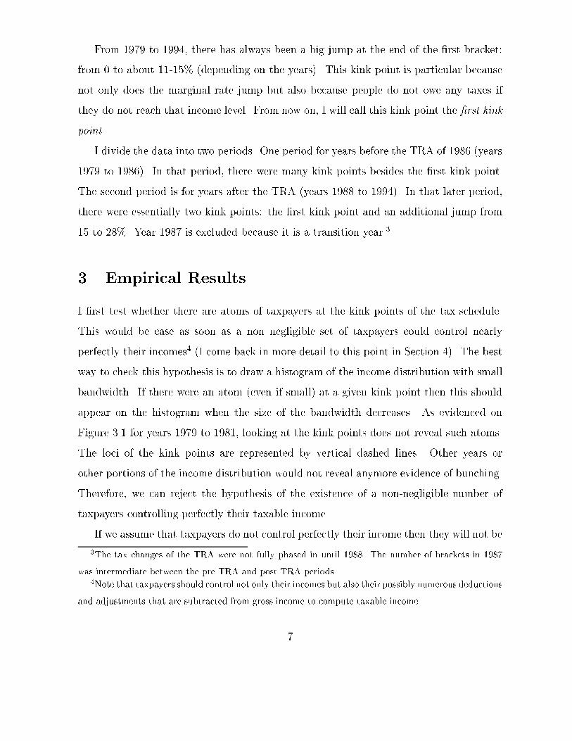
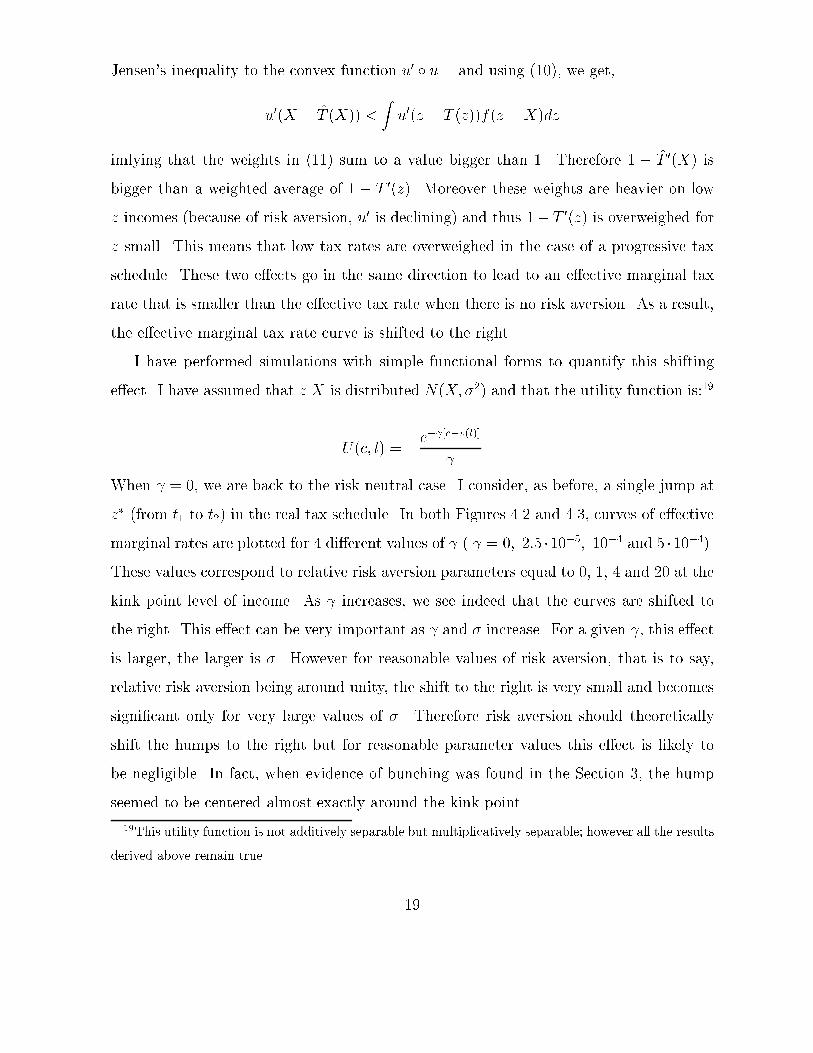
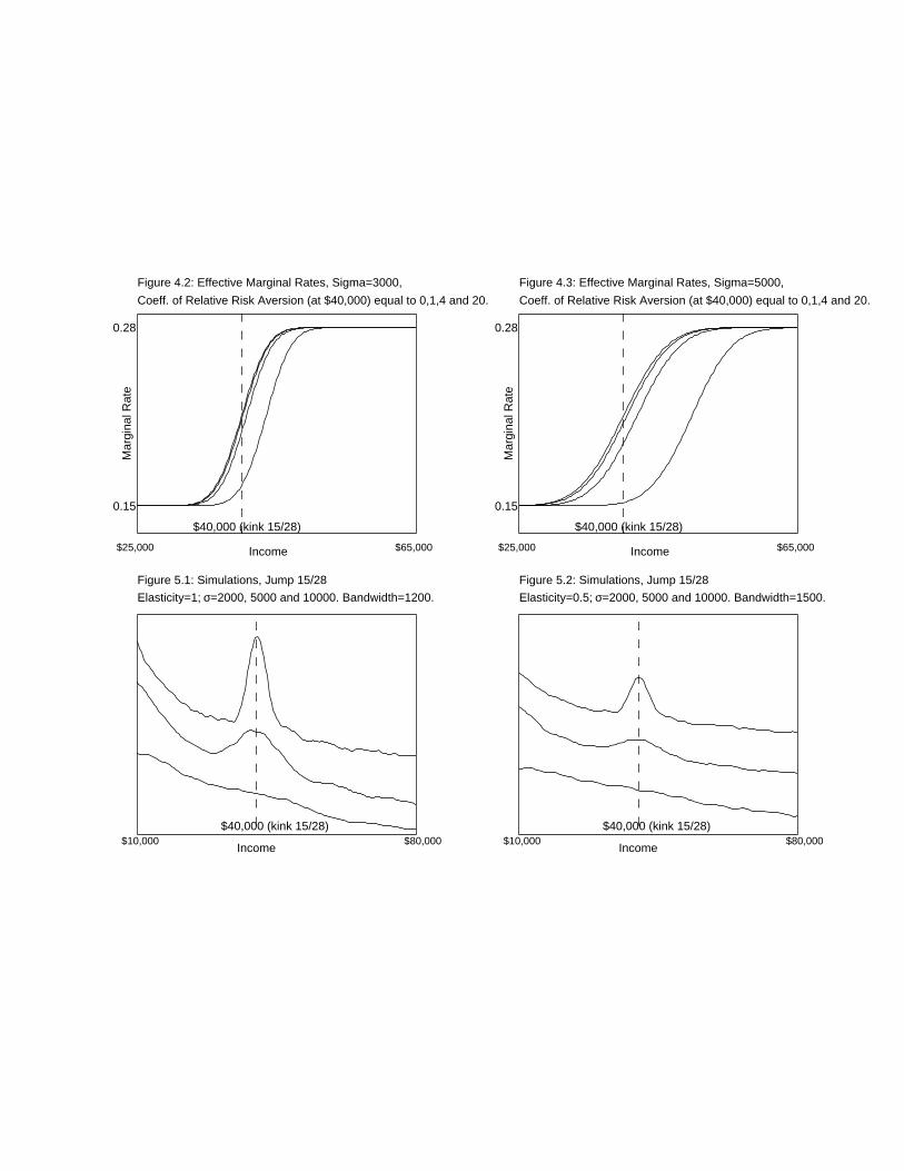
All these features are represented on Figures 4.2 and 4.3 in the special case of a jump
from 15 to 28% at income equal to 40,000 dollars and assuming that z = X + � with
� � N(0; �2). The curve corresponding to the risk neutral case in each panel is the one on
the left. It presents a point of in ection exactly at the kink point. This means that under
reasonable assumptions about the distribution of noise, we should expect to see the hump
of bunching exactly at the kink point. Comparing Figure 4.2 (� = 3; 000) and Figure 4.3
(� = 5; 000), we see that the smaller �, the sharper the increase in marginal rates.
� Risk Aversion
Let us now turn to the more complicated case with risk aversion. Using (7), the
e�ective tax schedule is given by,
X � T̂ (X) = u�1
�Zu(z � T (z))f(zjX)dz
�(10)
We can di�erentiate this expression with respect to X to derive the e�ective marginal
tax rate (assuming again that f(zjX) = f(z �X)),
1� T̂ 0(X) =
Z(1� T 0(z))
u0(z � T (z))
u0(X � T̂ (X))f(z �X)dz (11)
The e�ective net-of-tax rate is a weighted sum of real net-of-tax rates. However, in this
case, the weights are not simply f(z � X) but are multiplied by an additional factor
u0(z � T (z))=u0(X � T̂ (X)). If we assume realistically that u0 is convex18 then applying
18This is the case if taxpayers are prudent
18
Jensen's inequality to the convex function u0 � u�1 and using (10), we get,
u0(X � T̂ (X)) <
Zu0(z � T (z))f(z �X)dz
imlying that the weights in (11) sum to a value bigger than 1. Therefore 1 � T̂ 0(X) is
bigger than a weighted average of 1 � T 0(z). Moreover these weights are heavier on low
z incomes (because of risk aversion, u0 is declining) and thus 1� T 0(z) is overweighed for
z small. This means that low tax rates are overweighed in the case of a progressive tax
schedule. These two e�ects go in the same direction to lead to an e�ective marginal tax
rate that is smaller than the e�ective tax rate when there is no risk aversion. As a result,
the e�ective marginal tax rate curve is shifted to the right.
I have performed simulations with simple functional forms to quantify this shifting
e�ect. I have assumed that zjX is distributed N(X; �2) and that the utility function is:19
U(c; l) = �e� [c�v(l)]
When = 0, we are back to the risk neutral case. I consider, as before, a single jump at
z� (from t1 to t2) in the real tax schedule. In both Figures 4.2 and 4.3, curves of e�ective
marginal rates are plotted for 4 di�erent values of ( = 0; 2:5 �10�5; 10�4 and 5 �10�4).
These values correspond to relative risk aversion parameters equal to 0, 1, 4 and 20 at the
kink point level of income. As increases, we see indeed that the curves are shifted to
the right. This e�ect can be very important as and � increase. For a given , this e�ect
is larger, the larger is �. However for reasonable values of risk aversion, that is to say,
relative risk aversion being around unity, the shift to the right is very small and becomes
signi�cant only for very large values of �. Therefore risk aversion should theoretically
shift the humps to the right but for reasonable parameter values this e�ect is likely to
be negligible. In fact, when evidence of bunching was found in the Section 3, the hump
seemed to be centered almost exactly around the kink point.
19This utility function is not additively separable but multiplicatively separable; however all the results
derived above remain true.
19

We have studied the e�ect of uncertainty on the expected distribution of incomes
(nl(n)) but we are interested in the features of real income distributions. For a given
income nl, the realized income z is a random variable distributed according to f(zjnl)
and thus the humps in the distribution of realized incomes are further smoothed. As a
result, simulations of distributions of realized incomes z show that the variance of the
hump in the income distribution is about twice as large as the variance �2 of the random
process f(zjX).
4.3 Other models
The model with uncertainty analyzed previously does not capture all the features of the
e�ort supply decision. Many taxpayers cannot control perfectly the mean of their income
and probably face a limited menu of possible e�ort levels, each of these corresponding to
a di�erent type of job. For example, a Ph.D. graduate in economics can decide to take a
post-doc position or to become assistant professor or to become a consultant. Though it
is often possible to mix di�erent type of jobs, perfect �ne tuning of e�ort is impossible in
most cases. Low income earners who change jobs more frequently may adapt more easily
their work e�ort than high or middle income earners who stick to a given job for at least
one year once they have chosen an occupation.
A simple way to model this fact would be to assume that taxpayers face each year a
random menu of possible e�ort levels l, and that they choose in this limited menu the e�ort
level maximizing their utility. We can assume that taxpayers face each year independent
menus or more realistically that they can stick to the e�ort level of the previous year or
choose between new o�ers. In the later case, if the tax schedule does not change over
time, taxpayers are able to improve their utility as new o�ers appear year after year. In
the long run, each taxpayer will be able to reach his optimum level of e�ort. However,
even with the assumption of completely new menus each year, bunching appears in the
simulated income distributions as soon as the elasticity and the number of choices are not
too small. I present simulations using this model in Section 5.
20

Investment in human capital (along the lines of Becker (1975)) could also play an
important role: a bigger e�ort now not only increases my expected income today but
may also increase my ability level n in the subsequent periods. For example, young
consultants may have interest in working very hard not so much to increase their current
compensation but rather to increase their odds of being promoted and getting higher
wages in later periods. It is easy to see theoretically that if a bigger l has a positive e�ect
on n next period then bunching is reduced. Again, this investment feature is likely to
be more relevant for young high income earners rather than workers near retirement or
low income earners who change jobs frequently and never get tenure. This could explain
the di�erence in the results of low and middle-high income earners. Career concerns are
weaker in the case of low incomes and especially elderly getting social security bene�ts
and still working.20
5 Simulations
Qualitatively the theoretical models predict bunching, but we do not know yet what
quantity of bunching is to be found when realistic parameters are chosen. I address
this issue in this section. I �rst present the model, then a range of simulations results
and �nally I try to calibrate the parameters of the model to the true empirical income
distributions.
5.1 The Model
I have chosen very simple functional forms to make simulations. The basic utility function
chosen was introduced in Section 4.
U(c; l) = c�lk+1
k + 1
20That could also explain why Friedberg (1998) found clear evidence of bunching in that case.
21

This functional form is useful, because it allows explicit calculations. Moreover, the utility
is de�ned even for negative after tax incomes and so allows the use of normal distributions
for the random income e�ect. I use only utility functions with no risk aversion because
we have seen that the risk aversion e�ect is negligible for reasonable parameter values.
The noise in incomes is modeled using normal distributions. I assume that zjX follows a
law N(X; �2). There are two key parameters in this simple behavioral model.
1) e = k�1 represents the elasticity of income with respect to marginal net-of-tax rates.
Section 4 has shown that the amount of bunching is proportional to this elasticity.
2) � is the standard deviation of the stochastic process generating e�ective incomes.
For a given expected income X, the e�ective income lies with probability 0:95 in the
interval (X � 1:96�;X + 1:96�). In other words, � measures to what extent taxpayers
control their income.
In all simulations, these parameters are assumed to be constant in the population.
This is clearly unrealistic, but, once simulations are made for a range of parameters,
we could easily merge the simulated distributions to display cases where agents have
heterogeneous parameters. In order to make simulations, the e�ective tax schedule T̂ 0
must be computed. In the simple setting I consider, explicit formulas can be derived. I
then solve for the optimal e�ort. I can thus get a function which gives for every skill
n the corresponding expected income nl(n). It is then easy to draw the distribution of
n according to an underlying distribution g(n) and compute real realizations of incomes
z = nl+N(0; �2). Finally, I plot the distribution of incomes z using kernel density methods
as in Section 3. I can freely choose the size of the sample, thus I can get estimates close to
the asymptotic distribution. Therefore, I do not report asymptotic con�dence intervals.
5.2 Simulation results
In this subsection, I present some simulations to examine how the size of bunching
depends on the parameters previously described. For simplicity, I consider one single
22

jump in marginal rates from t1 to t2. In this subsection, I �rst consider a jump from 15
to 28% at the level of 40,000 dollars. and I assume that the distribution of n is uniform
around the kink point. This produces an income distribution comparable to the empirical
income distributions around the second kink point after the TRA. Simulated distributions
are represented on Figures 5.1 and 5.2. Simulations are plotted for elasticities equal to 1
(Figure 5.1) and 0.5 (Figure 5.2). I have performed simulations with 3 di�erent values of
�: � = 2000; 5000 and 10000 dollars. As was expected from our �ndings in Section 4,
the smaller � and the larger the elasticity, the sharper the humps. When the elasticity is
equal to one, even when � is equal to 10; 000, a at hump is still discernible. When the
elasticity decreases, smaller values of � are su�cient to eliminate completely the hump.
However, for reasonable values of �, which should be less than 5; 000 for many taxpayers
earning about 40; 000 dollars, the elasticity must be lower than 0.2-0.3 to make the hump
completely disappear. This implies that elasticities for middle income earners compatible
with the empirical results are much smaller than those derived by the studies of Lindsey
(1987) and Feldstein (1995). My results are consistent with the small elasticity results
found in the labor supply literature.
Evidence of bunching was found for married taxpayers at the �rst kink point where
the marginal rate jumps from 0 to 15 percent. At that point the density of income
distribution is still increasing and thus the assumption of n uniform is inaccurate. I
simulate a distribution of incomes closer to the real one using instead a normal distribution
for n. This produces a single peaked distribution for simulated incomes that matches
roughly the true empirical distribution of post 1986 years for married. The case of a at
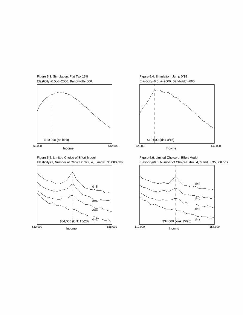
tax equal to 15% is shown on Figure 5.3.
Let us now introduce a kink point at the level of 10; 000 dollars where the marginal rate
jumps from 0 to 15% (as in the post TRA86 tax schedules). Figure 5.4 presents a simulated
distribution of incomes which matches the empirical bunching, the elasticity parameter is
equal to 0.5 and � = $2000. The kink point produces a deformation in the distribution
of incomes which is very similar to what is observed in the true empirical distributions.
23

Many low income earners probably can control their incomes pretty accurately, therefore
the assumption � = $2000 is reasonable. Lower values of � or higher elasticities would
produce humps bigger than in the empirical distribution. Therefore, these simulations
suggest that an elasticity equal to 0.5 is a reasonable upper bound for low income earners.
Table III (Panel A) summarizes those �ndings. The Table displays for the �rst and second
kink point and for a range of elasticities, the corresponding values of � that are required to
reproduce the evidence of bunching found in the empirical distributions. The number are,
of course, only indicative. They illustrate, however, clearly the fact that high elasticities
cannot be consistent with the empirical facts unless � is very large.
5.3 Model with limited menu of e�ort
An alternative theoretical model in which taxpayers can only choose their e�ort level l
from a limited random menu was presented in Section 4. In this subsection, I present
a few simulations to examine the quantitative properties of bunching in this model. I
consider the case of a single jump from 15 to 28% occurring at 40,000 dollars.
I assume that each taxpayer has to choose l in a random menu (l1; ::; ld). The li are
independent. For convenience, I assume that each li is distributed uniformly around a
fairly broad interval centered around the optimal e�ort level [(1 � �)n]1=k.21 Once l is
chosen, income is given by nl. e = k�1 represents the elasticity in the limiting case when
d is large. For d �nite, the true elasticity may not be exactly k�1 but is closely related to
that value.
Simulation results are given on Figure 5.5 for e = 1 and on Figure 5.6 for e = 0:5. For
both values of e, I present simulations for d = 2; 4; 6; 8. It appears clearly that bunching
increases with d and the elasticity e. For d = 2 bunching is hardly discernible (even
for e = 1), however bunching clearly appears once d � 4. Bunching is very sharp for
d = 8. As discussed in Section 4, it is reasonable to think that d increases overtime as
new o�ers appear while taxpayers can stick to their previous e�ort level. Therefore, we
21More precisely, this interval is (0:5n1=k; 1:7n1=k).
24
would expect d to be quite large after a few years. Thus again, this model is compatible
with empirical observations for middle income earners only if the elasticities of income
are small. It could well be possible that bunching is not discernible empirically because
there is both randomness of income realization and limited choice of l. However, even
in this mixed case, it would be di�cult to reconcile empirical results with high income
elasticities (elasticities bigger than 0.5). Table III (Panel B) displays the values of d that
are compatible with the empirical evidence for several values of the elasticity parameter.
5.4 Income Dynamics
The IRS has also built a panel of tax returns available from 1979 to 1990. It is of interest
to use it to have a more precise idea of income dynamics and get a rough idea of the size
of �. I have plotted distributions of di�erences in real taxable income for years 1987 to
1990 (post TRA) and di�erent portions of the income distribution.
In the model of taxation with uncertainty and stable preferences, taxpayers would
choose each year the same e�ort and thus di�erences in taxable income across two con-
secutive years would allow us to estimate �. For simplicity, if we assume as above that
zt = nl + �t with �t � N(0; �2) and independent across time, then zt � zt�1 � N(0; 2�2).
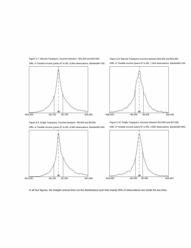
Distributions of di�erences in taxable income (zt � zt�1) are displayed on Figures 5.7 to
5.10. They are presented for two di�erent ranges of incomes (corresponding to the kinks
0/15 and 15/28 after 1986) for married and single taxpayers.22
From these density estimates, it is possible to estimate �. Table IV displays the
estimated values of �, computed as the standard deviation of the distribution zt � zt�1
(divided byp2). The estimation of � would be upward biased if preferences are not
constant over time; uctuations of income due to pure luck are likely to be smaller than
22I have computed di�erences in taxable income for two consecutive years and then merged the dif-
ferences corresponding to 1990-89, 1989-88 and 1988-87. Incomes have been normalized in 1991 dol-
lars. For example, Figure 5.7 represents the distribution of di�erences in incomes zt � zt�1 for incomes
zt�1 2 (�10000; 10000).
25

real uctuations. On the other hand, people may try to adapt their e�ort to smooth
income revenues, producing a downward bias in the estimate of �. The former e�ect is
likely to be stronger than the later and thus the estimation of � in Table IV are probably
biased upward.
As evidenced on Figures 5.7 to 5.10, many taxpayers experience small changes of
income across years. I have plotted on the Figures the income levels such that 50% of
taxpayers experience changes in income zt � zt�1 smaller than this level from year to
year. For example in Figure 5.7, 50% of taxpayers experience changes in income smaller
than 2,700 dollars. These levels are not very large and therefore we can think that
many taxpayers are able to control pretty accurately there incomes, therefore the absence
of bunching in the empirical distribution is more likely to be the consequence of small
elasticities than inability of taxpayers to control income.
The assumption of normality in the random component of incomes is inaccurate be-
cause the distributions on Figures 5.7 to 5.10 display too sharp a mode. This may mean
that the distribution of � is not homogeneous and that some taxpayers are able to control
very accurately their incomes. The model of limited choice of e�orts may also have some
relevance. We would then expect a very sharp mode because of people who stick to the
same level of e�ort. A mixed model of limited menu of e�ort with uncertainty could well
produce densities similar to the real ones.
6 Conclusion
This study has revealed clear evidence of bunching only at the �rst kink point. The
evidence for other kink points is either weak or null. These empirical results can be
explained within our theoretical framework in two ways. First, a large uncertainty in the
process generating incomes could make the humps around the kink points very at and
thus hard to observe in the data. Second, a small elasticity of income with respect to tax
rates for middle and high incomes earners would lead to small humps and therefore, no
26
clear evidence of clustering around the kink points in the data would be observed. Large
uncertainty of incomes is rejected by panel data evidence. Even if taxpayers cannot choose
freely their income target and have to select a job from a fairly limited menu of o�ers,
empirical income distribution should display clustering around the kinks if elasticities are
high.
Therefore, it is hard to reconcile these results with the very high elasticities estimated
by authors who looked directly at the e�ects of tax changes on taxable income (Feldstein
(1995) and Lindsey (1987)). These authors found elasticities bigger than 1 and sometimes
as high as 3. In all our models, such elasticities would produce large humps at kink points
for reasonable values of the remaining parameters. Moreover, those authors �nd higher
elasticities for high income earners than for low income earners. The present study sug-
gests the opposite. Elasticities seem to be signi�cant only for low income earners around
the �rst kink point. The present results are consistent with the small elasticity estimates
found in the traditional labor supply literature (see Pencavel (1986) for a survey). These
studies commonly �nd compensated elasticities around 0.2 which would not produce dis-
cernible bunching in the models I consider. However, the present study considers taxable
income and thus should capture all the dimensions of e�ort (as in Feldstein's and Lindsey's
studies) and not only hours of work. One reason could explain this discrepency. Lindsey
and Feldstein are not able to control for time e�ects in a fully convincing way: they rely
on the fact that high incomes have increased faster than low incomes between 1981 and
1985 (Lindsey) and between 1985 and 1988 (Feldstein) and relate this fact to the decrease
in tax rates during both periods. But it is generally acknowledged that this increase in
inequalities could have other sources. For example, Murphy and Welch (1992) and Katz
and Murphy (1992) found that the returns to human capital or education increased as a
result of increased demand for skilled labor. The approach used here does not su�er from
this problem. However, my results are essentially qualitative and it is beyond the scope
of this paper to provide precise estimates. Several recent studies have estimated elastic-
ities of taxable income using other tax changes or better datasets than the ones used by
27

Feldstein and Lindsey. These new studies ( Auten-Carroll (1997), Goolsbee (1997), Saez
(1997) among others) are able to control for underlying increases in inequality and �nd
much smaller elasticities (below 0.6) which are consistent with the results presented in
this study.
This study also casts some doubts on the relevance of the approach of non-linear budget
sets to estimate the e�ects of taxes on labor supply (Hausman (1981)). Uncertainty
smoothes the kinks of the budget set and therefore it is not correct to add an error
term in the labor supply equation (see Section 1) without modifying the shape of the
budget set. Therefore, it would be very interesting to reconsider the non-linear budget
set methodology with a smoothed budget set and see whether this a�ects the results.
MaCurdy, Green and Paarsch (1990) already used a smoothed budget set in this type of
study but mainly to simplify calculations. It should be possible to choose a smoothed
budget set consistent with the variance of the error term in order to test the relevance of
the nonlinear-budget set methodology.
The results of this paper suggest other directions for future research. First, it would
be interesting to replicate the empirical estimations presented here to income tax sched-
ules of other countries. Some countries have very progressive tax schedules generating
big jumps in marginal rates23 and therefore looking at taxable income distributions for
these countries may bring additional evidence about bunching behavior. Second, welfare
programs in the US generate big kinks in the budget set.24 The bene�ciaries are mostly
low income earners. Therefore it would be interesting to estimate the distribution of in-
comes of recipients of these programs and see whether there is evidence of bunching at
kink points.25 These programs sometimes introduce even discontinuities in the budget
23France, for example, has an income tax schedule with only seven brackets with top marginal rate
equal to 56%.
24Usually the bene�ts are taxed away at very high rates above an exemption level.25Kane (1998) has looked for bunching in the case of a program of saving incentives for higher education.
The schedule of bene�ts induces a large kink in the budget set of participants. However, Kane was not
able to �nd any evidence of bunching.
28

set (known as notches) which should generate even more clustering. For example, the
study of the Medicaid Notch (Yelowitz (1995)) could be enriched by application of non-
parametric methods. This could corroborate our result of signi�cant elasticities for low
income earners.
29

Appendix
Econometric Methodology
The data set is a strati�ed sample, so each observation (taxable income xi) is associated
with a weight (denoted wi). The weights are normalized to sum to one. Assume that the
sample is of size N , the usual kernel density formula is given by:
f̂h(x) =1
h
NXi=1
K(x� xi
h)wi
where h is the bandwidth and K is the kernel function. For all the estimations, I used
the Epanechnikov kernel function:
K(u) =3
4(1� u2)I(juj < 1)
The choice of the kernel function does not change the shape of the estimates, that is
why I stick to this simple kernel function. Let us assume that the underlying true density
distribution is given by f and that f is at least twice continuously di�erentiable. The
expectation of f̂h(x) in the case of Epanechnikov functions can be approximated by:
E[f̂h(x)] = f(x) +1
10h2f 00(x) + o(h2)
The variance of f̂h(x) can be approximated by:
V ar[f̂h(x)] =3
5N�hf(x) + o(
1
N�h)
with N� = (PN
i=1w2i )
�1 (N� = N when all the weights are equal26). So when h ! 0,
E[f̂h(x)] ! 0 and when N�h ! 1, V ar[f̂h(x)] ! 0. Thus theoretically, if f is smooth
enough, the kernel estimate has good properties of convergence. From those results, it
is easy to derive the asymptotic distribution of the kernel estimate: when h ! 0 and
N�h!1
26In general, the weights in the sample are such that N� is about 3
4N .
30

pN�h(f̂h(x)� f(x))! N(0;
3
5f(x))
A 95% asymptotic point-wise con�dence interval is given by:
0B@f̂h(x)� 1:96
"3f̂h(x)
5N�h
# 12
; f̂h(x) + 1:96
"3f̂h(x)
5N�h
# 12
1CA (12)
Note that this con�dence interval is accurate only asymptotically. All the con�dence
intervals plotted with the curve estimates are 95 % asymptotic con�dence intervals com-
puted using formula (12). All these derivations are presented in more detail in Hardle
(1990).
Data Aggregation
In some cases, estimates merging several years are presented. The aim is to improve
the accuracy of the estimates by increasing the number of observations.
Years from 1988 to 1994 are merged so as to superpose exactly the two relevant kink
points: jump from 0 to 15% at taxable income 0, and jump from 15 to 28%. As the tax
schedule was indexed to in ation during those years, taxable income is simply de ated.
The estimates are normalized in year 1991 dollars.
Years 1979,1980 and 1981 are merged directly because tax schedules were not indexed
and therefore the kinks remain at the same location in nominal terms. For years 1982 to
1986, we have proceeded as follows. From year 1982 to 1984, the loci of the kink point did
not change, but tax rates have decreased: the same kink points do not correspond to the
same jumps in marginal taxes. Therefore, we have merged these years directly with years
1979 to 1981. Years 1985 and 1986 tax schedules are indexed by a simple multiplicative
factor; therefore, by dividing incomes by these multiplicative factors, we can make all the
kink points match. Results for these years are normalized in year 1984 dollars.
31

References
[1] Auten, Gerald and Robert Carroll. \The E�ect of Income Taxes on Household Be-
havior." O�ce of Tax Analysis, U.S. Department of the Treasury, mimeo 1997, forth-
coming Review of Economics and Statistics.
[2] Becker, Gary. Human Capital, Chigago University Press, 1975.
[3] Burtless, Gary and Jerry Hausman, \The E�ect of Taxation on Labor Supply: Eval-
uating the Gary Income Maintenance Experiment," Journal of Political Economy,
1978, 86, pp. 1103-1130.
[4] Burtless, Gary and Robert Mo�t, \The E�ect of Social Security Bene�ts on the
Labor Supply of the Aged." In Aaron, H. and G. Burtless, eds., Retirement and
Economic Behavior. Washington: Brookings Institution, 1984.
[5] Deaton, Angus. Understanding Consumption Oxford University Press, 1992.
[6] Feldstein, Martin. \The E�ect of Marginal Tax Rates on Taxable Income: A Panel
Study of the 1986 Tax Reform Act" Journal of Political Economy, 1995, 103(3) pp.
551-572.
[7] Friedberg, Leora. \The Social Security Earnings Test and Labor Supply of Older
Men." in Tax Policy and the Economy, vol. 12, ed. J. Poterba. Cambridge: MIT
Press, 1998.
[8] Goolsbee, Austan. \What Happens When You Tax the Rich? Evidence from Exec-
utive Compensation.", NBER Working Paper, No. 6333, 1997.
[9] Hardle, Wolfgang. Applied non-parametric regression, Cambridge University Press,
1990.
[10] Hausman, Jerry. \Labor Supply", in How Taxes A�ect Economic Behavior, ed. Henry
J. Aaron and Joseph A. Pechman. Washington, D.C.: Brookings Institution, 1981.
32

[11] Hausman, Jerry. \Stochastic Problems in the Simulation of Labor Supply". in M.
Feldstein, ed., Behavioral Simulations in Tax Policy Analysis, University of Chicago
Press, 1982, pp. 41-69.
[12] Heckman, James. \Comment". in M. Feldstein, ed., Behavioral Simulations in Tax
Policy Analysis University of Chicago Press, 1982, pp. 70-82.
[13] Kane, Thomas. \Saving Incentives for Higher Education." National Tax Journal,
1998, 51(3), pp. 609-20.
[14] Katz, Lawrence and Kevin Murphy. \Changes in Relative Wages, 1963-1987: Supply
and Demand Factors." Quarterly Journal of Economics, 1992, 107, pp. 35-78.
[15] Liebman, Je�rey. \The Impact of the Earned Income Tax Credit on Incentives and
Income Distribution.", in Tax Policy and the Economy, vol. 12, ed. J. Poterba. Cam-
bridge: MIT Press, 1998.
[16] Lindsey, Lawrence. \Individual Taxpayer Response to Tax Cuts: 1982-1984, with
Implications for the Revenue Maximizing Tax Rate." Journal of Public Economics,
1987, (33), pp. 173-206.
[17] MaCurdy, Thomas, David Green and Harry Paarsch. \Assessing Empirical Ap-
proaches for Analyzing Taxes and Labor Supply." The Journal of Human Resources,
Fall 1990, pp. 415-490.
[18] Mirrlees, James. \An Exploration in the Theory of Optimal Income Taxation" Review
of Economic studies, 1971, 38, pp. 175-208.
[19] Mirrlees, James. \Untended Labor Supply." Mimeo Nu�eld College, 1980.
[20] Mo�t Robert, \The Econometrics of Kinked Budget Constraints." Journal of Eco-
nomic Perspectives, 1990, 4(2), pp. 119-139.
33

[21] Murphy, Kevin and Finis Welch. \The Structure of Wages." Quarterly Journal of
Economics, 1992, 107(1), pp. 285-326.
[22] Pencavel, John. \Labor Supply of Men." in O. Ashenfelter and R. Layard (eds.),
Handbook of Labor Economics, 1986, Amsterdam: North-Holland, pp. 3-102.
[23] Saez, Emmanuel. \The E�ect of Marginal Tax Rates on Income: A Panel Study of
`Bracket Creep'.", MIT mimeograph, 1997.
[24] Yelowitz, Aaron. \The Medicaid Notch, Labor Supply and Welfare Participation:
Evidence from Eligibility Expansions" Quaterly Journal of Economics, 1995, 105,
pp. 909-940.
34

</ref_section>
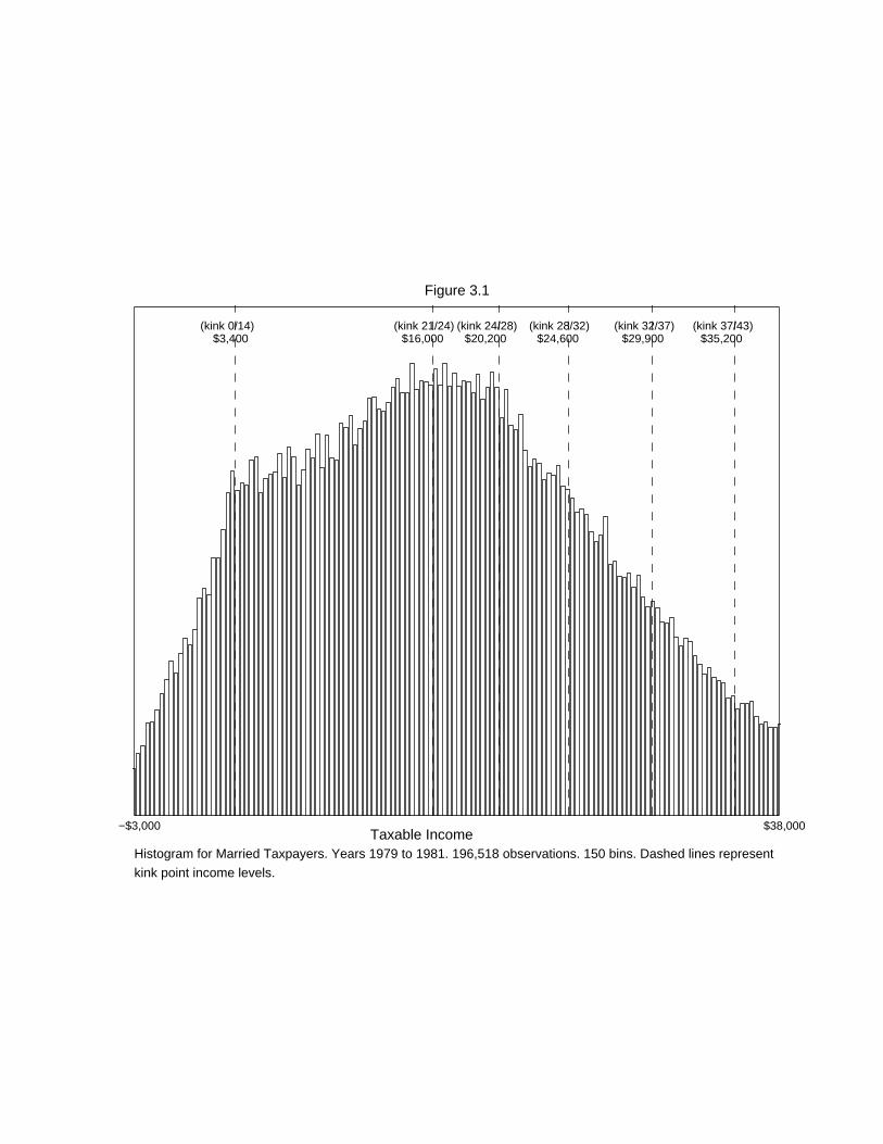
Figure 3.1
−$3,000 $38,000
$3,400(kink 0/14)
$29,900(kink 32/37)
$24,600(kink 28/32)
$35,200(kink 37/43)(kink 24/28)
$20,200$16,000(kink 21/24)
Taxable IncomeHistogram for Married Taxpayers. Years 1979 to 1981. 196,518 observations. 150 bins. Dashed lines represent
kink point income levels.
−$3,000 $38,000
$3,400(kink 0/14)
$29,900(kink 32/37)
$24,600(kink 28/32)
$35,200(kink 37/43)
(kink 24/28)$20,200
$16,000(kink 21/24)
Taxable Income
Figure 3.2: Married Taxpayers
Years 1979 to 1986. 317,804 observations. Bandwidth=1000.
−$13,000 $58,000$0 (kink 0/15) $34,000 (kink 15/28)
Taxable Income in 91 dollars
Years 1988 to 1994. 194,186 observations. Bandwidth=1500.
Figure 3.3: Married Taxpayers
−$13,000 $58,000$0 (kink 0/15) $34,000 (kink 15/28)
Taxable Income in 91 dollars
Year 1988. 23,659 observations. Bandwidth=2300.
Figure 3.4: Married Taxpayers
−$13,000 $58,000$0 (kink 0/15) $34,000 (kink 15/28)
Taxable Income in 91 dollars
Year 1994. 27,000 observations. Bandwidth=2300.
Figure 3.5: Married Taxpayers
−$3,000 $28,000
$2,300(kink 0/14)
$10,800(kink 21/24)
$15000(kink 26/30)
$18,200(kink 30/34)
$23,500(kink 34/39)
Taxable Income
Figure 3.6: Single Taxpayers.
Years 1979 to 1986. 149,284 observations. Bandwidth=700.
−$8,000 $38,000$0 (kink 0/15) $20,350 (kink 15/28)
Taxable Income in 91 dollars
Figure 3.7: Single Taxpayers
Years 1988 to 1994. 101,194 observations. Bandwidth=1200.
−$8,000 $38,000$0 (kink 0/15) $20,350 (kink 15/28)
Taxable Income in 91 dollars
Figure 3.8: Single Taxpayers
Year 1988. 13,745 observations. Bandwidth=1600.
−$8,000 $38,000$0 (kink 0/15) $20,350 (kink 15/28)
Taxable Income in 91 dollars
Figure 3.9: Single Taxpayers
Year 1994. 14,368 observations. Bandwidth=1600.
−$9,000 $39,000
$0 (kink(0/15)
Taxable Income
Figure 3.10: Married Taxpayers: all observations
Year 1993. 20,096 observations. Bandwidth=1000.
−$9,000 $39,000
$0 (kink(0/15)
Taxable Income
Figure 3.11: Married Taxpayers Expecting RefundYear 1993. 12,534 observations. Bandwidth=1000.
$37,000 $59,000
$45,800 (kink(43/49)
Taxable Income
Figure 3.12: Married Taxpayers
Years 1979 to 1986. 94,725 observations. Bandwidth=600.
$46,000 $64,000
$55,300 (kink(55/63)
Taxable Income
Figure 3.13: Single Taxpayers
Years 1979 to 1981. 2,585 observations. Bandwidth=1000.
−$13,000 $58,000$0 (kink 0/15) $34,000 (kink 15/28)
Taxable Income in 91 dollars
Years 1987 to 1994. 123,684 observations. Bandwidth=1800.
Figure 3.14: Married Taxpayers. Itemizers
−$13,000 $58,000$0 (kink 0/15) $34,000 (kink 15/28)
Taxable Income in 91 dollars
Years 87 to 94. 70,502 observations. Bandwidth=2000.
Figure 3.15: Married Taxpayers. Non−Itemizers
−$8,000 $38,000$0 (kink 0/15) $20,350 (kink 15/28)
Taxable Income in 91 dollars
Figure 3.16: Single Taxpayers. Itemizers
Years 1988 to 1994. 39,629 observations. Bandwidth=1500.
−$8,000 $38,000$0 (kink 0/15) $20,350 (kink 15/28)
Taxable Income in 91 dollars
Figure 3.17: Single Taxpayers. Non−Itemizers
Years 1988 to 1994. 61,565 observations. Bandwidth=1500.
Before Tax Income
Afte
r T
ax In
com
e
Figure 4.1: Theoretical Bunching
z* z*+dz*
slope 1−t−dt
Individual L
indifference curve
slope 1−t
Individual H
indifference curves
dz*/z*=e dt/(1−t)
Mar
gina
l Rat
e
$25,000 $65,000
0.15
0.28
$40,000 (kink 15/28)
Income
Coeff. of Relative Risk Aversion (at $40,000) equal to 0,1,4 and 20.
Figure 4.2: Effective Marginal Rates, Sigma=3000,
Mar
gina
l Rat
e
$25,000 $65,000
0.15
0.28
$40,000 (kink 15/28)
Income
Coeff. of Relative Risk Aversion (at $40,000) equal to 0,1,4 and 20.
Figure 4.3: Effective Marginal Rates, Sigma=5000,
$10,000 $80,000$40,000 (kink 15/28)
Income
Elasticity=1; σ=2000, 5000 and 10000. Bandwidth=1200.
Figure 5.1: Simulations, Jump 15/28
$10,000 $80,000$40,000 (kink 15/28)
Income
Elasticity=0.5; σ=2000, 5000 and 10000. Bandwidth=1500.
Figure 5.2: Simulations, Jump 15/28
$10,000 (no kink)
$42,000$2,000Income
Elasticity=0.5; σ=2000. Bandwidth=600.
Figure 5.3: Simulation, Flat Tax 15%
$10,000 (kink 0/15)
$42,000$2,000Income
Elasticity=0.5; σ=2000. Bandwidth=600.
Figure 5.4: Simulation, Jump 0/15
$12,000 $58,000
$34,000 (kink 15/28)
Income
d=2
d=4
d=6
d=8
Elasticity=1, Number of Choices: d=2, 4, 6 and 8. 35,000 obs.
Figure 5.5: Limited Choice of Effort Model
$12,000 $58,000
$34,000 (kink 15/28)
Income
d=2
d=4
d=6
d=8
Elasticity=0.5; Number of Choices: d=2, 4, 6 and 8. 35,000 obs.
Figure 5.6: Limited Choice of Effort Model
−$18,000 $18,000$0
−$2,700 $2,700
Figure 5.7: Married Taxpayers, Incomes between −$10,000 and $10,000,
Diffs. in Taxable Income (years 87 to 90). 6,854 observations. Bandwidth=700.
−$30,000 $30,000$0
−$4,300 $4,300
Figure 5.8: Married Taxpayers Incomes between $24,000 and $44,000,
Diffs. in Taxable Income (years 87 to 90). 7,364 observations. Bandwidth=700.
−$14,000 $14,000$0
−$2,100 $2,100
Figure 5.9: Single Taxpayers, Incomes between −$5,000 and $5,000,
Diffs. in Taxable Income (years 87 to 90). 6,083 observations. Bandwidth=500.
In all four figures, the straight vertical lines cut the distributions such that exactly 50% of observations are inside the two lines.
−$19,000 $19,000$0
−$2,400 $2,400
Figure 5.10: Single Taxpayers, Incomes between $13,000 and $27,000,
Diffs. in Taxable Income (years 87 to 90). 4,695 observations. Bandwidth=800.

Table I: Tax Table,
Years 1979 to 1981
Taxable Income Jump in Tax Rates Net-of-Tax Ratio Taxable Income Jump in Tax Rates Net-of-Tax Ratio(1) (2) (3) (4) (5) (6)
$3,400 0/14 0.860 $2,300 0/14 0.860
$5,500 14/16 0.977 $3,400 14/16 0.977
$7,600 16/18 0.976 $4,400 16/18 0.976
$11,900 18/21 0.963 $6,500 18/19 0.988
$16,000 21/24 0.962 $8,500 19/21 0.975
$20,200 24/28 0.947 $10,800 21/24 0.962
$24,600 28/32 0.944 $12,900 24/26 0.974
$29,900 32/37 0.926 $15,000 26/30 0.946
$35,200 37/43 0.905 $18,200 30/34 0.943
$45,800 43/49 0.895 $23,500 34/39 0.924
$60,000 49/54 0.902 $28,800 39/44 0.918
$85,600 54/59 0.891 $34,100 44/49 0.911
$109,400 59/64 0.878 $41,500 49/55 0.882
$162,400 64/68 0.889 $55,300 55/63 0.822
$215,400 68/70 0.937 $81,800 63/68 0.865
$108,300 68/70 0.937
Notes: The Table shows the nominal levels of kink points (taxable income), the tax rate levels and the corresponding net-of-tax ratios.
Single TaxpayersMarried Taxpayers Filing Jointly
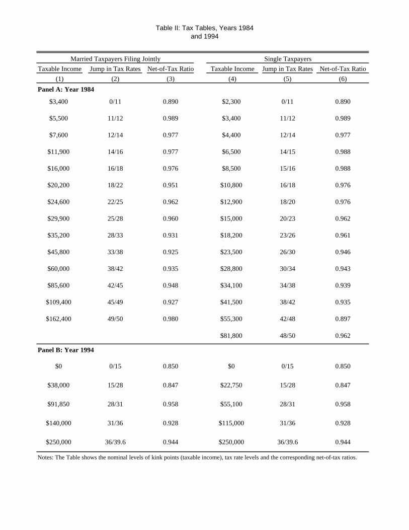
Table II: Tax Tables, Years 1984and 1994
Taxable Income Jump in Tax Rates Net-of-Tax Ratio Taxable Income Jump in Tax Rates Net-of-Tax Ratio
(1) (2) (3) (4) (5) (6)
Panel A: Year 1984
$3,400 0/11 0.890 $2,300 0/11 0.890
$5,500 11/12 0.989 $3,400 11/12 0.989
$7,600 12/14 0.977 $4,400 12/14 0.977
$11,900 14/16 0.977 $6,500 14/15 0.988
$16,000 16/18 0.976 $8,500 15/16 0.988
$20,200 18/22 0.951 $10,800 16/18 0.976
$24,600 22/25 0.962 $12,900 18/20 0.976
$29,900 25/28 0.960 $15,000 20/23 0.962
$35,200 28/33 0.931 $18,200 23/26 0.961
$45,800 33/38 0.925 $23,500 26/30 0.946
$60,000 38/42 0.935 $28,800 30/34 0.943
$85,600 42/45 0.948 $34,100 34/38 0.939
$109,400 45/49 0.927 $41,500 38/42 0.935
$162,400 49/50 0.980 $55,300 42/48 0.897
$81,800 48/50 0.962
Panel B: Year 1994
$0 0/15 0.850 $0 0/15 0.850
$38,000 15/28 0.847 $22,750 15/28 0.847
$91,850 28/31 0.958 $55,100 28/31 0.958
$140,000 31/36 0.928 $115,000 31/36 0.928
$250,000 36/39.6 0.944 $250,000 36/39.6 0.944
Notes: The Table shows the nominal levels of kink points (taxable income), tax rate levels and the corresponding net-of-tax ratios.
Married Taxpayers Filing Jointly Single Taxpayers

Table III: Calibration Results
(1) (2) (3) (4) (5) (6)
Panel A: Model with Random Incomes
ElasticityParameter e 0.25 0.5 1 0.25 0.5 1
Compatible Standard deviation σ $1,500 $2,000 $5,000 $6,000 $8,000 $12,000
Panel B: Model with limited menu of effort levels
ElasticityParameter e 0.25 0.5 1 0.25 0.5 1
Compatible Number ofChoices d d=8 d=6 d=4 d=4 d=3 d=2
Notes: The Table displays, for each value of the elasticity e, the corresponding value of the standard deviation σ (Panel A) and the number of choices d (Panel B) required to reproduce the bunching observed in empirical distributions in the simulations. Numbers displayed are based on Figures 5.1-5.6 and are only indicative.
Second Kink Point 15/28First Kink Point 0/15

Table IV: Estimates of σ from Panel Data
Taxable Income Range Estimate of σ Taxable Income Range Estimate of σ
(1) (2) (3) (4)
$-10,000 to $10,000 $3,500 $-5,000 to $5,000 $2,500
$24,000 to $44,000 $5,200 $13,000 to $27,000 $3,900
Notes: Estimates of σ are computed from the distribution of differences in taxable income z(t+1)-z(t) for z(t) in the range given in columns (1) and (3).
Married Taxpayers Filing Jointly Single Taxpayers