Embed Size (px)
Citation preview

DO-TH 17/19
CP3-Origins-2017-055 DNRF90
Neutrinoless Double Beta Decay and
the Baryon Asymmetry of the Universe
Frank F. Deppisch1∗, Lukas Graf 1†, Julia Harz2‡, Wei-Chih Huang3,4§
1Department of Physics and Astronomy, UCL, Gower Street, London WC1E 6BT, UK2Sorbonne Universites, Institut Lagrange de Paris, 98bis Blvd. Arago, F-75014 Paris; Sorbonne
Universites, UPMC Univ Paris 06 & CNRS, UMR 7589, LPTHE, F-75005 Paris; France3 Fakultat fur Physik, Technische Universitat Dortmund, 44221 Dortmund, Germany
4CP3-Origins, University of Southern Denmark, Campusvej 55, DK-5230 Odense M, Denmark
Abstract
We discuss the impact of the observation of neutrinoless double beta decay on the
washout of lepton number in the early universe. Neutrinoless double beta decay can be
triggered by a large number of mechanisms that can be encoded in terms of Standard
Model effective operators which violate lepton number by two units. We calculate
the contribution of such operators to the rate of neutrinoless double beta decay and
correlate it with the washout of lepton number induced by the same operators in
the early universe. We find that the observation of a non-standard contribution to
neutrinoless double beta decay, i.e. not induced by the standard mass mechanism of
light neutrino exchange, would correspond to an efficient washout of lepton number
above the electroweak scale for many operators up to mass dimension 11. Combined
with Standard Model sphaleron transitions, this would render many baryogenesis
mechanisms at higher scales ineffective.
∗E-mail: [email protected]†E-mail: [email protected]‡E-mail: [email protected]§E-mail: [email protected]
1
arX
iv:1
711.
1043
2v1
[he
p-ph
] 2
8 N
ov 2
017
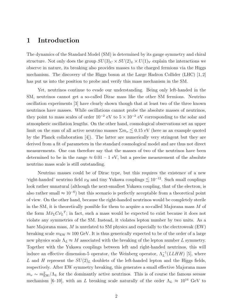
1 Introduction
The dynamics of the Standard Model (SM) is determined by its gauge symmetry and chiral
structure. Not only does the group SU(3)C × SU(2)L × U(1)Y explain the interactions we
observe in nature, its breaking also provides masses to the charged fermions via the Higgs
mechanism. The discovery of the Higgs boson at the Large Hadron Collider (LHC) [1, 2]
has put us into the position to probe and verify this mass mechanism in the SM.
Yet, neutrinos continue to evade our understanding. Being only left-handed in the
SM, neutrinos cannot get a so-called Dirac mass like the other SM fermions. Neutrino
oscillation experiments [3] have clearly shown though that at least two of the three known
neutrinos have masses. While oscillations cannot probe the absolute masses of neutrinos,
they point to mass scales of order 10−2 eV to 5× 10⁻² eV corresponding to the solar and
atmospheric oscillation lengths. On the other hand, cosmological observations set an upper
limit on the sum of all active neutrino masses Σmν . 0.15 eV (here as an example quoted
by the Planck collaboration [4]). The latter are numerically very stringent but they are
derived from a fit of parameters in the standard cosmological model and are thus not direct
measurements. One can therefore say that the masses of two of the neutrinos have been
determined to be in the range ≈ 0.01 – 1 eV, but a precise measurement of the absolute
neutrino mass scale is still outstanding.
Neutrino masses could be of Dirac type, but this requires the existence of a new
‘right-handed’ neutrino field νR and tiny Yukawa couplings . 10−12. Such small couplings
look rather unnatural (although the next-smallest Yukawa coupling, that of the electron, is
also rather small ≈ 10−6) but this scenario is perfectly acceptable from a theoretical point
of view. On the other hand, because the right-handed neutrinos would be completely sterile
in the SM, it is theoretically possible for them to acquire a so-called Majorana mass M of
the form MνLCνLT ; in fact, such a mass would be expected to exist because it does not
violate any symmetries of the SM. Instead, it violates lepton number by two units. As a
bare Majorana mass, M is unrelated to SM physics and especially to the electroweak (EW)
breaking scale mEW ≈ 100 GeV. It is thus generically expected to be of the order of a large
new physics scale ΛL ≈M associated with the breaking of the lepton number L symmetry.
Together with the Yukawa couplings between left and right-handed neutrinos, this will
induce an effective dimension-5 operator, the Weinberg operator, Λ−1L (LLHH) [5], where
L and H represent the SU(2)L doublets of the left-handed lepton and the Higgs fields,
respectively. After EW symmetry breaking, this generates a small effective Majorana mass
mν ∼ m2EW/ΛL for the dominantly active neutrinos. This is of course the famous seesaw
mechanism [6–10], with an L breaking scale naturally of the order ΛL ≈ 1014 GeV to
2

achieve the light neutrino masses mν ≈ 0.1 eV.
While certainly the most prominent case, the above scenario is just one example of
how the effective L-violating Weinberg operator and thus a Majorana mass for the active
neutrinos can be generated; at the tree level there are two further generic ways, via triplet
scalars and fermions, respectively, and there are numerous other ways at higher loop order
and when allowing higher-dimensional effective interactions beyond the Weinberg operator.
What these models have in common is that in order to generate light Majorana masses
for the active neutrinos, L needs to be broken. This symmetry, along with baryon number
B symmetry, is accidentally conserved in the SM at the perturbative level. Weak non-
perturbative instanton and sphaleron effects through the chiral Adler-Bell-Jackiw anomaly
[11,12] do in fact violate baryon and lepton number but only in the combination (B+L) [13].
The ‘orthogonal’ combination (B−L) remains conserved and thus lepton number violation
(LNV), or more generally (B−L) violation, along with the generation of Majorana neutrino
masses requires the presence of New Physics beyond the SM (BSM).
In this context, a clear hint for physics beyond the SM is the observation of a baryon
asymmetry of our Universe, quantified in terms of the baryon-to-photon number density [14]
ηobsB = (6.20± 0.15)× 10−10 . (1)
In order to generate a baryon asymmetry the three Sakharov conditions have to be ful-
filled, namely (1) B violation, (2) C and CP violation and (3) out-of-equilibrium dynamics.
Different approaches exist which exhibit these conditions, one popular scenario is baryoge-
nesis via leptogenesis (LG) [15]. In the standard “vanilla” scenario, a right handed heavy
neutrino decays out of equilibrium via a lepton number violating decay and introduces a
new source of CP violation. As long as this happens before the EW phase transition, the
lepton asymmetry is translated into a baryon asymmetry.
While the violation of lepton number is a crucial ingredient e.g. in the leptogenesis
scenario, in order to satisfy the third Sakharov condition, the LNV interactions must not
be too efficient. Otherwise they remove the lepton number asymmetry and, due to the
presence of sphaleron transitions in the SM, also the baryon number asymmetry before it
is frozen in at the EW breaking scale. The search for LNV processes, with neutrinoless
double beta (0νββ) as the most prominent example, therefore provides a potential pathway
to probe or rather falsify certain baryogenesis scenarios, if the lepton number washout in
the early universe can be correlated with the LNV process rate. In this paper, we take a
model-independent approach and study SM invariant operators of mass dimension 5, 7, 9
and 11 that violate lepton number by two units, ∆L = 2. We correlate their contribution to
0νββ, either at tree level or induced by radiative effects, with the lepton number washout
3

in the early universe. Assuming the observation of 0νββ decay, where we take the expected
sensitivity of T 0νββ1/2 ≈ 1027 y of future 0νββ experiments, we determine the temperature
range where the corresponding lepton number washout is effective.
After the discovery of the sphaleron transitions, the constraint on LNV operators
from the requirement to protect the observed baryon asymmetry was soon realized [16]
with the Weinberg operator as the most prominent example [16–22]. More generic non-
renormalizable operators were discussed in [19, 20] while the argument can also be ex-
tended to baryon number violating ∆B = 2 operators inducing neutron-antineutron os-
cillations [23, 24]. More recently, we have shown in [25] that searches for resonant LNV
processes at the LHC can be used to infer strong lepton number washout and in [26, 27]
we have demonstrated the principle to correlate the washout rate with non-standard 0νββ
contributions. In this paper we discuss the latter approach in more detail and extend the
analysis to more than the four example operators previously analyzed. Clearly, more strin-
gent constraints on the scale of baryogenesis can be derived in specific models. For example,
in left-right symmetric scenarios, the gauge interaction felt by the right-handed neutrinos
inducing leptogenesis will lead to a more rapid equilibration and thus strong constraints
on the left-right breaking scale [28,29].
The paper is organized as follows. In Section 2, we discuss basic properties of 0νββ.
Section 3 provides a list of effective SM invariant operators up to dimension 11 that violate
lepton number by two units. These form the basis of the subsequent discussion, which first
deals with contributions to 0νββ from such effective operators in Section 4. It describes an
algorithm we employ to estimate the radiative generation of operators that trigger 0νββ
decay. Section 5 then describes the washout of lepton number in the early Universe by an
effective operator. In Section 6 we correlate the washout with 0νββ decay, and determine
the temperature range in the thermal history where a given operator effectively washes out
lepton number under the assumption that it triggers 0νββ decay at an observable rate. We
discuss the results and comment on potential caveats in Section 7.
2 Neutrinoless Double Beta Decay
The search for 0νββ decay, i.e. the decay of an even-even nucleus emitting two electrons,
for example in the case of the Xenon isotope 13654Xe,
13654Xe→ 136
56Ba + e−e−, (2)
is the most sensitive tool for probing Majorana neutrino masses. However, while this
so-called mass mechanism is certainly the best known that triggers the decay, Majorana
4
d
d u
e-
e-
GF
GF
u
O5
(a)
h0
h0
d
d u
e-
e-
GF
uO7
νL
(b)
h0
d
d
u
u
e-
e-
O9
(c)
d
d
u
u
e-
e-
O11
(d)
h0
h0
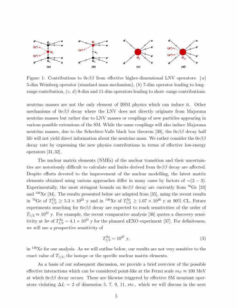
Figure 1: Contributions to 0νββ from effective higher-dimensional LNV operators: (a)
5-dim Weinberg operator (standard mass mechanism), (b) 7-dim operator leading to long–
range contribution, (c, d) 9-dim and 11-dim operators leading to short–range contributions.
neutrino masses are not the only element of BSM physics which can induce it. Other
mechanisms of 0νββ decay where the LNV does not directly originate from Majorana
neutrino masses but rather due to LNV masses or couplings of new particles appearing in
various possible extensions of the SM. While the same couplings will also induce Majorana
neutrino masses, due to the Schechter-Valle black box theorem [30], the 0νββ decay half
life will not yield direct information about the neutrino mass. We rather consider the 0νββ
decay rate by expressing the new physics contributions in terms of effective low-energy
operators [31, 32].
The nuclear matrix elements (NMEs) of the nuclear transition and their uncertain-
ties are notoriously difficult to calculate and limits derived from 0νββ decay are affected.
Despite efforts devoted to the improvement of the nuclear modelling, the latest matrix
elements obtained using various approaches differ in many cases by factors of ∼(2 − 3).
Experimentally, the most stringent bounds on 0νββ decay are currently from 76Ge [33]
and 136Xe [34]. The results presented below are adapted from [35], using the recent results
in 76Ge of TGe1/2 ≥ 5.3 × 1025 y and in 136Xe of TXe
1/2 ≥ 1.07 × 1026 y at 90% CL. Future
experiments searching for 0νββ decay are expected to reach sensitivities of the order of
T1/2 ≈ 1027 y. For example, the recent comparative analysis [36] quotes a discovery sensi-
tivity at 3σ of TXe1/2 = 4.1× 1027 y for the planned nEXO experiment [37]. For definiteness,
we will use a prospective sensitivity of
TXe1/2 = 1027 y, (3)
in 136Xe for our analysis. As we will outline below, our results are not very sensitive to the
exact value of T1/2, the isotope or the specific nuclear matrix elements.
As a basis of our subsequent discussion, we provide a brief overview of the possible
effective interactions which can be considered point-like at the Fermi scale mF ≈ 100 MeV
at which 0νββ decay occurs. These are likewise triggered by effective SM invariant oper-
ators violating ∆L = 2 of dimension 5, 7, 9, 11, etc., which we will discuss in the next
5

section. Fig. 1 shows the contribution of such operators schematically. For more details on
the effective 0νββ, see the review [35] and references therein. General up-to-date reviews
of 0νββ decay and associated physics can be found in [38], while a more specific recent
review on 0νββ NMEs is available in [39].
Standard Mass Mechanism Before discussing the exotic contributions of our interest,
we remind the reader that the mass mechanism of 0νββ decay is sensitive to the effective
Majorana neutrino mass
mν =3∑j=1
U2ejmνj ≡ mee, (4)
where the sum runs over all active light neutrinos with masses mνj , weighted by the square
of the charged-current leptonic mixing matrix U . This quantity is equal to the (ee) entry
of the Majorana neutrino mass matrix. The inverse 0νββ decay half life in a given isotope
is then given by
T−11/2 =
∣∣∣∣mν
me
∣∣∣∣2G0|Mν |2, (5)
where G0 is the nuclear phase space factor and |Mν | the corresponding NME. The effective
Majorana neutrino mass is normalized with respect to the electron mass me to yield a
small dimensionless parameter εν = mν/me, comparable between different contributions.
The current experimental results lead to a limitmν . 0.06−0.17 eV [34] with an uncertainty
due to the nuclear matrix elements. Future experiments will aim to probe mν ≈ 0.02 eV.
Additional Long-Range Contributions to 0νββ decay involve two vertices with the
exchange of a light neutrino in between, cf. Fig. 1 (b). The general Lagrangian can be
written in terms of effective couplings εαβ [31],
L =GF√
2
(jµV−AJ
†V−A,µ +
∑α,β
εβαjβJ†α
), (6)
where jβ = eOβν and J†α = uOαd are the leptonic and hadronic currents, respectively.
The sum runs over all possible Lorentz-invariant combinations with right-handed leptonic
currents where the standard case α = β = (V − A) is shown separately. All currents
are conventionally scaled relative to the strength of the ordinary (V −A) interaction, GF ,
via the dimensionless ε factors. The operators Oα in Eq. (6) are OV±A = γµ(1 ± γ5),
OS±P = (1± γ5) and OTR|L = i2[γµ, γν ](1± γ5).
6

|ε| × 108 εν εV+AV−A εV+A
V+A εS+PS±P εTRTR ε1 ε2 εa3 εb3 ε4 ε5
76Ge 41 0.21 37 0.66 0.07 19 0.11 1.30 0.83 0.90 9.076Xe 26 0.11 22 0.26 0.03 10 0.05 0.43 0.66 0.46 4.6
Table 1: Upper limits on effective 0νββ interactions (in units of 10−8) from the current
experimental bounds TGe1/2 & 5.3× 1025 y and TXe
1/2 & 1.07× 1026 y. Only one ε is assumed
to be present at a time. The coupling εν = mν/me is due to the standard mechanism with
the corresponding limits on the effective 0νββ mass of 0.21 eV (Ge) and 0.13 eV (Xe). For
the short-range interaction ε3, the limit depends on the chirality of the hadronic currents:
εa3 (hadronic currents have same chirality), εb3 (hadronic currents have opposite chirality).
Table adapted from [35].
Short–range contributions to 0νββ decay involve a single effective interaction of
dimension-9, cf. Fig.1 (c,d). The possible operators are [32]
L =G2F
2mp
(ε1JJj + ε2JµνJµνj + ε3J
µJµj + ε4JµJµνj
ν + ε5JµJjµ) , (7)
with the hadronic currents J = u(1 ± γ5)d, Jµ = uγµ(1 ± γ5)d, Jµν = u i2[γµ, γν ](1 ± γ5)d
and the leptonic currents j = e(1 ± γ5)eC , jµ = eγµ(1 ± γ5)eC . The operators are scaled
with respect to a point-like, double beta decay-like interaction with the proton mass mp.
In our subsequent analysis the different non-standard operators, either long-range
or short-range, originate from SM invariant LNV operators, themselves understood to be
generated in a specific BSM scenario. Considering one operator with associated εβα at a
time, the inverse 0νββ half life can be expressed as
T−11/2 = |εβα|2G0k|Mαβ|2, (8)
analogous to the standard case, where G0k denotes the corresponding nuclear phase space
factors and |Mαβ| the nuclear matrix elements, which depend both on the isotope as well
the operator in question. Using the approach of [35], the current limits on the effective
0νββ interaction are shown in Tab. 11.
Having in mind the generation of the above long-range and short-range 0νββ inter-
actions from effective SM gauge-invariant LNV operators and ultimately from new physics
where lepton number is broken at a high scale ΛLNV, we neglect several effects. A complete
scheme would include the QCD running and consequently generation of color-mismatched
operators [41–44]. At the QCD scale, operators should be matched to chiral EFT [45] and
1Compared to [35], we omit the interaction εTR
TL, which was shown to vanish [40].
7
pion-induced transitions can in fact be dominant for short-range interactions, compared to
the usually considered four-nucleon transitions. As already mentioned, the matrix elements
calculated in nuclear structure theories continue to have large uncertainties. Despite the
importance of such effects, we do not anticipate that our results depend on them strongly.
This is because the underlying SM invariant operators that we consider are of dimension
D = 7, 9, 11, and thus the uncertainty in the nuclear matrix element only enters as the third
root for D = 7, ΛD=7LNV ∝ 3
√|M |, and even weaker for the higher-dimensional operators.
3 Survey of LNV operators
So far the most exhaustive (but by no means complete) list of SM effective operators violat-
ing lepton number by two units has been published in [46], based on an initial enumeration
in [47]. In [26] we studied four different operators contributing at tree-level to 0νββ decay.
In the following we will extend our study to all ∆L = 2 operators up to dimension-9 and a
representative fraction of dimension-11 operators. Most of the operators will not contribute
directly at tree-level, but at various loop levels. Our goal is to study the contribution of
all these operators to the effective 0νββ interactions, as depicted in Fig. 1.
In order to convince ourselves we are not missing important operators, we generate
∆L = 2 operator patterns using the Hilbert Series method [48]. This top-to-bottom ap-
proach to effective field theories is able to provide all possible independent operator patterns
(i.e. solely the field content of particular operators, not the structure of contractions) that
can be formed using a specified particle content respecting given symmetries. The series
encodes also the multiplicity of each such pattern, and therefore the total number of in-
dependent effective operators allowed under considered constraints can be easily obtained.
This ensures that we capture all possible ∆L = 2 operators involving SM fermions and
the Higgs. As in [46], we omit operators involving gauge fields and derivatives and we are
interested just in the possible SU(2) contractions, which means we do not take into account
all the possible Lorentz and SU(3) structures; we instead show the multiplicity introduced
by these degrees of freedom. In general, we specify the effective operators considering just a
single generation of fermions, but additionally, we also list possible SU(2) contractions that
are only allowed if more fermionic generations are taken into account. The resulting sets of
operators of dimensions 7, 9 and 11 are listed in Tabs. 4, 5 and 6, respectively, in addition
to single Weinberg operator of dimension-5 in Eq. 11. Therefore, all the interactions we
consider can be schematically summarized in a Lagrangian
L = LSM +1
Λ5
O5 +∑i
1
Λ37i
Oi7 +∑i
1
Λ59i
Oi9 +∑i
1
Λ711i
Oi11, (9)
8

Leptons Quarks Higgs Boson
Label Rep Label Rep Label Rep
L =
(νL
eL
) (1, 2,−1
2
)Q =
(uL
dL
) (3, 2, 1
6
)H =
(h+
h0
) (1, 2, 1
2
)ec (1, 1, 1)
uc(3, 1,−2
3
)dc
(3, 1, 1
3
)Table 2: Notation used to label the corresponding representations of the fermions and the
Higgs field of the SM given in the form (SU(3)c, SU(2)L, U(1)Y ).
where LSM stands for the SM Lagrangian, O5 is the unique Weinberg operator of dimension-
5 suppressed by the corresponding typical energy scale Λ5 andOiD are the other SM effective
operators of higher dimensions D = 7, 9, 11 suppressed by ΛD−4Di
. All the effective scales
ΛDi subsume any mass scales and couplings of an underlying UV-complete theory. In our
calculations we will always consider just a single effective operator in addition to the SM
Lagrangian at a time.
The notation used for the fields the considered effective operators consist of is sum-
marized in Tab. 3, where all the listed fermions are left-handed 2-component Weyl spinors.
The right-handed hermitian conjugates are denoted by a bar, e.g. the conjugate partner
for the electron singlet ec reads ec. The 2-component Weyl spinors used in this section are
related to the 4-component spinors used e.g. in Eqs. (6) and (7) as
ν =
(νL
νL
), e =
(eL
ec
), u =
(uL
uc
), d =
(dL
dc
), (10)
where e, u, d are Dirac spinors, while ν is a Majorana spinor.
3.1 Dimension 5
At dimension-5, there is a single ∆L = 2 operator (modulo generations). The Hilbert series
confirms this and reads
H∆L=25 = L2H2 + h.c.. (11)
As noted, the Hilbert series method does not provide the actual Lorentz and gauge con-
tractions involved in an operator. It is merely a polynomial in the given fields. The above
of course corresponds to the unique Weinberg operator
O1 = LiLjHkH lεikεjl, (12)
9
O Operator mν LR εLR
1H 2LiLjHkH lH
tHtεikεjl
v2
Λ f(vΛ
)− −
2 LiLjLkecH lεijεklye
16π2v2
Λ − −3a LiLjQkdcH lεijεkl
ydg2
(16π2)2v2
Λv
Λ3 εS+PS+P
3b LiLjQkdcH lεikεjlyd
16π2v2
Λv
Λ3 εS+PS+P
4a LiLjQiucHkεjk
yu16π2
v2
Λv
Λ3 εS+PS−P
4∗b LiLjQk ucH k εijyug2
(16π2)2v2
Λv
Λ3 εS+PS−P
8 LiecucdcHjεijyexe ydyu
(16π2)2v2
Λv
Λ3 2εV+AV+A
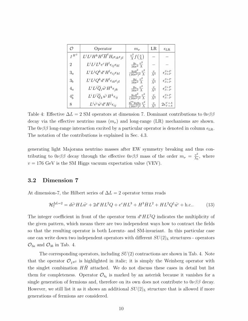
Table 4: Effective ∆L = 2 SM operators at dimension 7. Dominant contributions to 0νββ
decay via the effective neutrino mass (mν) and long-range (LR) mechanisms are shown.
The 0νββ long-range interaction excited by a particular operator is denoted in column εLR.
The notation of the contributions is explained in Sec. 4.3.
generating light Majorana neutrino masses after EW symmetry breaking and thus con-
tributing to 0νββ decay through the effective 0νββ mass of the order mν = v2
Λ5, where
v = 176 GeV is the SM Higgs vacuum expectation value (VEV).
3.2 Dimension 7
At dimension-7, the Hilbert series of ∆L = 2 operator terms reads
H∆L=27 = decHLuc + 2dcHL2Q+ ecHL3 +H3HL2 +HL2Q†uc + h.c.. (13)
The integer coefficient in front of the operator term dcHL2Q indicates the multiplicity of
the given pattern, which means there are two independent ways how to contract the fields
so that the resulting operator is both Lorentz- and SM-invariant. In this particular case
one can write down two independent operators with different SU(2)L structures - operators
O3a and O3b in Tab. 4.
The corresponding operators, including SU(2) contractions are shown in Tab. 4. Note
that the operator O1H2 is highlighted in italic; it is simply the Weinberg operator with
the singlet combination HH attached. We do not discuss these cases in detail but list
them for completeness. Operator O4b is marked by an asterisk because it vanishes for a
single generation of fermions and, therefore on its own does not contribute to 0νββ decay.
However, we still list it as it shows an additional SU(2)L structure that is allowed if more
generations of fermions are considered.
10

3.3 Dimension 9
Similarly, at dimension-9, the Hilbert series of ∆L = 2 operator terms reads
H∆L=29 =(dc)2 dcL2uc +(dc)2 ec2uc2 + 2(dc)2 ecLQuc + 4(dc)2 L2Q2 + dcececL2uc
+ 2dcecL3Q+ dcecH2HLuc + 2dcecLQuc2 + 3dcH2HL2Q+ dcL3Luc + 4dcL2QQuc
+ dcL2ucuc2 + dcH3L2Q+(ec)2 L4 + ecH2HL3 + ecL3Quc + ecH3L2L+ ecH3LQQ
+H4H2L2 +H3L2Quc + 2H2HL2Quc + 2L2Q
2uc2 + h.c.. (14)
The corresponding effective operators are listed in Tab. 5. For completeness we again
list operators ‘derived’ from lower-dimensional ones, such as O1H4 which is the Weinberg
operator with the singlet combinationHH attached twice orO1ye which is also the Weinberg
operator with the singlet combination LHec attached. We do not discuss these operators
in detail. Operator O12b is marked by an asterisk (similarly as operator O4b shown for
dimension 7), as it vanishes for a single generation of fermions and as such it does not
contribute to 0νββ decay. It is also worth noting that the operator O76 does not appear
in [46].
3.4 Dimension 11
As the number of operators of dimension 11 is quite large and many of them behave in a
similar manner we restrict our calculations to the selection shown in Tab. 6. It includes all
11-dimensional operators that trigger 0νββ at tree level but we omit for example operators
that do not appreciably contribute to 0νββ through long-range or short-range interactions.
4 Contributions to Neutrinoless Double Beta Decay
To determine the contributions of the operators listed in the previous section to 0νββ
decay, we start by identifying those which trigger this rare nuclear process at tree level.
Clearly, the Weinberg operator O1 is such an operator through the effective neutrino mass,
cf. Fig. 1 (a). At higher dimensions, the following operators trigger 0νββ directly after
EW symmetry breaking,
Dimension-7 : O3a, O3b, O4a, O4b, O8; (15)
Dimension-9 : O5, O6, O7, O11b, O12a, O14b, O19, O20; (16)
Dimension-11: O24a, O28a, O28c, O32a, O36, O37, O47a, O47d,
O53, O54a, O54d, O55a, O59, O60. (17)
11

O Operator mν LR εLR SR εSR
1H4LiLjHkHlH
tHtH
uHuεikεjl
v2
Λf2
(vΛ
)− − − −
1 ye LiLjHkHl(LtHtec)εikεjl
ye(16π2)2
v2
Λ− − − −
1 yd LiLjHkHl(QtHtdc)εikεjl
yd(16π2)2
v2
Λ
ydyexd|u
16π2v
Λ3 f(vΛ
)εS+PS±P − −
2H2LiLjLkecHlH
tHtεijεkl
ye16π2
v2
Λf(vΛ
)− − − −
3H2
a LiLjQkdcHlHtHtεijεkl
ydg2
(16π2)2v2
Λf(vΛ
)v
Λ3 f(vΛ
)εS+PS+P − −
3H2
b LiLjQkdcHlHtHtεikεjl
yd16π2
v2
Λf(vΛ
)v
Λ3 f(vΛ
)εS+PS+P − −
4H2
a LiLjQiucHkH
tHtεjk
yu16π2
v2
Λf(vΛ
)v
Λ3 f(vΛ
)εS+PS−P − −
5 LiLjQkdcHlHmHiεjlεkmyd
(16π2)2v2
Λv
Λ3 f(vΛ
)εS+PS+P − −
6 LiLjQkucHlHkHiεjl
yu(16π2)2
v2
Λv
Λ3 f(vΛ
)εS+PS−P − −
7 LiQj ecQkHkHlHmεilεjm
yexe g2
(16π2)2v2
Λf(vΛ
)v3
Λ5 2εV +AV−A − −
8H2LiecucdcHjH
tHtεij
yexe ydyu(16π2)2
v2
Λf(vΛ
)v
Λ3 f(vΛ
)2εV +A
V +A − −
9 LiLjLkecLlecεijεkly2e
(16π2)2v2
Λ− − − −
10 (2) LiLjLkecQldcεijεklyeyd
(16π2)2v2
Λye
16π2v
Λ3 εS+PS+P − −
11a (2) LiLjQkdcQldcεijεkly2dg
2
(16π2)3v2
Λyd
16π2v
Λ3 εS+PS+P
g2
16π21
Λ5 ε1
11b (2) LiLjQkdcQldcεikεjly2d
(16π2)2v2
Λyd
16π2v
Λ3 εS+PS+P
1Λ5 ε1
12a LiLjQiucQj uc
y2u(16π2)2
v2
Λyu
16π2v
Λ3 εS+PS−P
1Λ5 ε1
12∗b LiLjQkucQlu
cεijεkl y2ug
2
(16π2)3v2
Λyu
16π2v
Λ3 εS+PS−P
g2yexd yexu(16π2)2
1Λ5 ε1
13 LiLjQiucLlecεjl
yeyu(16π2)2
v2
Λye
16π2v
Λ3 εS+PS−P − −
14a (2) LiLjQkucQkdcεij
ydyug2
(16π2)3v2
Λ
yu|d16π2
vΛ3 εS+P
S±Pg2
(16π2)21
Λ5 ε1
14b (2) LiLjQiucQldcεjl
ydyu(16π2)2
v2
Λ
yu|d16π2
vΛ3 εS+P
S±P1
Λ5 ε1
15 LiLjLkdcLiucεjkydyug
2
(16π2)3v2
Λ
g2yexu|d|e(16π2)2
vΛ3 εS+P
S±P |2εV +AV +A − −
16 LiLjecdcecucεijydyug
4
(16π2)4v2
Λye
16π2v
Λ3 2εV +AV +A − −
17 LiLjdcdcdcucεijydyug
4
(16π2)4v2
Λ
g2yexu|d|e(16π2)2
vΛ3 εS+P
S±P |2εV +AV +A
yexd yexe16π2
1Λ5 2ε5
18 LiLjdcucucucεijydyug
4
(16π2)4v2
Λ
g2yexu|d|e(16π2)2
vΛ3 εS+P
S±P |2εV +AV +A
yexe yexu16π2
1Λ5 2ε5
19 (2) LiQjdcdcecucεijyexe y2dyu(16π2)3
v2
Λyd
16π2v
Λ3 2εV +AV +A
1Λ5 2ε5
20 (2) LidcQiucecuc
yexe ydy2u
(16π2)3v2
Λyu
16π2v
Λ3 2εV +AV +A
1Λ5 2ε5
61 LiLjHkHlLrecHrεikεjlye
16π2v2
Λf(vΛ
)− − − −
66 LiLjHkHlεikQrdcHrεjl
yd16π2
v2
Λf(vΛ
)1
16π2v
Λ3 εS+PS+P − −
71 LiLjHkHlQrucHsεrsεikεjlyu
16π2v2
Λf(vΛ
) yuyexd|u
16π2v
Λ3 f(vΛ
)εS+PS±P − −
76 ececdcdcucucyex2e y2dy
2u
(16π2)4v2
Λ
ydyuyexe
(16π2)2v
Λ3 2εV +AV +A
1Λ5 2εLLz3
Table 5: Effective ∆L = 2 SM operators at dimension 9. Dominant contributions to 0νββ
decay via the effective neutrino mass (mν) as well as long-range (LR) and short-range (SR)
mechanisms are shown. The 0νββ long-range and short-range interactions excited by a
particular operator are denoted in column εLR and εSR. The notation of the contributions
is explained in Sec. 4.3.
They contribute as in Fig. 1 (b), (c) and (d), respectively, except the dim-9 operators O5,
O6 and O7 which trigger long-range interactions at tree level after all three Higgs fields
12

O Operator mν LR εLR SR εSR
21a LiLjLkecQlucHmHnεijεkmεlnyeyu
(16π2)2v2
Λf(vΛ
) yeyexe yexu
(16π2)2v3
Λ5 2εV +AV−A − −
21b LiLjLkecQlucHmHnεilεjmεknyeyu
(16π2)2v2
Λf(vΛ
) yeyexe yexu
(16π2)2v3
Λ5 2εV +AV−A − −
23 LiLjLkecQkdcHlHmεilεjm
yeyd(16π2)2
v2
Λf(vΛ
) yexd|(e)yexd ye
(16π2)2v
Λ3 f(vΛ
)εS+PS−P |εV +A
V +A − −24a LiLjQkdcQldcHmHiεjkεlm
y2d(16π2)3
v2
Λyd
16π2v
Λ3 f(vΛ
)εS+PS+P
1Λ5 f
(vΛ
)ε1
24b LiLjQkdcQldcHmHiεjmεkly2d
(16π2)3v2
Λyd
16π2v
Λ3 f(vΛ
)εS+PS+P
g2
(16π2)1
Λ5 f(vΛ
)ε1
25 LiLjQkdcQlucHmHnεimεjnεklydyu
(16π2)2v2
Λf(vΛ
) yu(16π2)2
vΛ3 εS+P
S+P
yex2u(16π2)2
1Λ5 ε1
26a LiLjQkdcLiecHlHmεjlεkm
yeyd(16π2)3
v2
Λye
16π2v
Λ3 f(vΛ
)εS+PS+P − −
26b LiLjQkdcLk ecHlHmεilεjm
yeyd(16π2)2
v2
Λf(vΛ
) ye(16π2)2
vΛ3 εS+P
S+P − −27a LiLjQkdcQid
cHlHmεjlεkmg2
(16π2)3v2
Λyd
16π2v
Λ3 f(vΛ
)εS+PS+P
yex2d(16π2)2
1Λ5 ε1
27b LiLjQkdcQkdcHlHmεilεjm
g2
(16π2)3v2
Λyd
(16π2)2v
Λ3 εS+PS+P
yex2d(16π2)2
1Λ5 ε1
28a LiLjQkdcQj ucHlHiεkl
ydyu(16π2)3
v2
Λyu
16π2v
Λ3 f(vΛ
)εS+PS+P
v2
Λ7 ε1
28b LiLjQkdcQkucHlHiεjl
ydyu(16π2)3
v2
Λ
yu|d16π2
vΛ3 f
(vΛ
)εS+PS±P
g2
(16π2)1
Λ5 f(vΛ
)ε1
28c LiLjQkdcQlucHlHiεjk
ydyu(16π2)3
v2
Λyd
16π2v
Λ3 f(vΛ
)εS+PS−P
1Λ5 f
(vΛ
)ε1
29a LiLjQkucQkucHlHmεilεjm
g2
(16π2)3v2
Λyu
(16π2)2v
Λ3 εS+PS−P
yexd yexu(16π2)2
1Λ5 ε1
29b LiLjQkucQlucHlHmεikεjm
g2
(16π2)3v2
Λyu
16π2v
Λ3 f(vΛ
)εS+PS−P
yexd yexu(16π2)2
1Λ5 ε1
30a LiLjLiecQkucHkHlεjl
yeyu(16π2)3
v2
Λye
16π2v
Λ3 f(vΛ
)εS+PS−P − −
30b LiLjLmecQnucHkHlεikεjlε
mn yeyu(16π2)2
v2
Λf(vΛ
) ye(16π2)2
vΛ3 εS+P
S−P − −31a LiLjQid
cQkucHkHlεjl
ydyu(16π2)2
v2
Λf(vΛ
) yd16π2
vΛ3 f
(vΛ
)εS+PS−P
yex2d(16π2)2
1Λ5 ε1
31b LiLjQmdcQnu
cHkHlεikεjlεmn ydyu
(16π2)2v2
Λf(vΛ
) yd(16π2)2
vΛ3 εS+P
S−P
yex2d(16π2)2
1Λ5 ε1
32a LiLjQj ucQku
cHkHiy2u
(16π2)3v2
Λyu
16π2v
Λ3 f(vΛ
)εS+PS−P
1Λ5 f
(vΛ
)ε1
32b LiLjQmucQnu
cHkHiεjkεmn y2u
(16π2)3v2
Λyu
16π2v
Λ3 f(vΛ
)εS+PS−P
yex2d(16π2)2
1Λ5 ε1
34 ececLiQjecdcHkHlεikεjlyexe ydg
2
(16π2)4v2
Λ
g2yexe|u|(d)(16π2)2
vΛ3 f
(vΛ
)εS+PS+P |2εV +A
V±A − −
35 ececLiecQj ucHjHkεik
yexe yug2
(16π2)4v2
Λ
g2yexe|d|(u)
(16π2)2v
Λ3 f(vΛ
)εS+PS−P |2εV +A
V±A − −
36 ececQidcQjdcHkHlεikεjlyex2e y2dg
2
(16π2)5v2
Λ
ydyexe yexe|u|(d)
(16π2)2v
Λ3 f(vΛ
)εS+PS+P |2εV +A
V±A1
Λ5 f(vΛ
)ε1
37 ececQidcQj ucHjHkεik
yex2e ydyug2
(16π2)5v2
Λ
g2yexe(16π2)2
v3
Λ5 2εV +AV +A
1Λ5 f
(vΛ
)ε1
38 ececQiucQj u
cHiHj yex2e y2ug2
(16π2)5v2
Λ
yexe|d|(u)yexe yu
(16π2)2v
Λ3 f(vΛ
)εS+PS−P |2εV +A
V±A1
Λ5 f(vΛ
)ε1
40a LiLjLkQlLiQjHmHnεkmεln
g2
(16π2)3v2
Λ
g2yexd|u|u|e(16π2)2
vΛ3 f
(vΛ
)εS+PS±P |2εV +A
V±A − −
43a LiLjLkdcLlucHlHiεjk
ydyug2
(16π2)4v2
Λ
g2yexu|d|e(16π2)2
vΛ3 f
(vΛ
)εS+PS±P |2εV +A
V +A − −44c LiLjQkecQle
cHlHmεijεkmg4
(16π2)4v2
Λye
16π2v3
Λ5 εV+AV−A − −
47a LiLjQkQlQiQjHmHnεkmεln
g2
(16π2)3v2
Λ
g2yexd|u|(e)(16π2)2
vΛ3 f
(vΛ
)εS+PS±P |2εV +A
V−Av2
Λ7 2εa3
47d LiLjQkQlQiQmHmHnεjkεln
g2
(16π2)3v2
Λ
g2yexd|u|(e)(16π2)2
vΛ3 f
(vΛ
)εS+PS±P |2εV +A
V−Av2
Λ7 2εa3
53 LiLjdcdcucucHiHjy2dy
2ug
2
(16π2)5v2
Λ
ydyuyexu|d|e
(16π2)2v
Λ3 f(vΛ
)εS+PS±P |2εV +A
V +Av2
Λ7 2εa3
54a LiQjQkdcQiecHlHmεjlεkm
yexe ydg2
(16π2)4v2
Λ
g2yexe|(d)|u(16π2)2
vΛ3 f
(vΛ
)εS+PS+P |2εV +A
V∓A − −54d LiQjQkdcQle
cHlHmεijεkmyexe ydg
2
(16π2)4v2
Λyd
16π2v3
Λ5 εV +AV−A
v2
Λ7 2ε5
55a LiQjQiQk ecucHkHlεjl
yexe yug2
(16π2)4v2
Λyu
16π2v3
Λ5 εV +AV−A
v2
Λ7 2ε5
59 LiQjdcdcecucHkHiεjkyexe y2dyu(16π2)4
v2
Λyd
(16π2)2v
Λ3 εV +AV +A
1Λ5 f
(vΛ
)2ε5
60 LidcQj ucecucHjHi
yexe ydy2u
(16π2)4v2
Λyu
(16π2)2v
Λ3 εV +AV +A
1Λ5 f
(vΛ
)2ε5
Table 6: As Tab. 5 but showing selected effective ∆L = 2 SM operators at dimension 11.
13

acquire their vacuum expectation value. In order to estimate the contribution of a single
D-dimensional operator to 0νββ decay, we consider radiative corrections to all other LNV
operators of the same and lower dimension. This implies a huge number of possibilities in
reducing a single operator such that we utilize an algorithm as outlined below.
4.1 SU(2) Decomposition and Effective 0νββ Couplings
To understand how the ∆L = 2 SM effective operators contribute at low energy to 0νββ
decay, we first decompose them into the SU(2) components. As a result, for each operator
we obtain 2d/2 components, where d is the number of SU(2) doublets present in the given
operator. For example, the operator O3a splits into 4 different SU(2) components,
O3a = LiLjQkdcH lεijεkl = νLeLuLh0dc − eLνLuLh0dc − νLeLdLh+dc + eLνLdLh
+dc. (18)
The ∆L = 2 SM effective operators contributing to 0νββ decay at tree level must corre-
spond in the broken phase to one of the terms in the effective 0νββ decay Lagrangians
in Eqs. (6) and (7), which e.g. means that the SU(2)L-components in Eq. (18) including
h0 can be (after EW symmetry breaking) mapped to one of the terms in Eq. (6). Con-
tributions to 0νββ decay triggered by other operators contributing to 0νββ decay at loop
level are determined by finding their relation to the tree-level-contributing ones, which will
be achieved by employing the algorithmic approach described later on. The effective cou-
plings ε appearing in Eqs. (6) and (7) can be restricted by current limits on the 0νββ decay
half-life. For this we relate the broken-phase contributions to those triggered by the SM
effective operators and obtain thus bounds on the new physics scales Λ suppressing the SM
effective operators. To identify these relations among unbroken-phase and broken-phase
contributions we proceed as follows.
4.1.1 6D Long-Range Contributions
Let us first focus on ∆L = 2 SM effective operators that trigger (after EW symmetry
breaking) the long-range contributions to 0νββ decay at tree level. Using the above list
of the tree-level-contributing SM effective operators, applying the SU(2) decomposition,
breaking the phase and checking the non-vanishing components we conclude there are in
total 7 such operators. Each of them corresponds in the broken phase to one of four different
6-dimensional low-energy 0νββ decay operators (all formed by 4 relevant fermions - u, d,
14
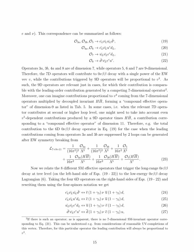
e and ν). This correspondence can be summarized as follows:
O3a,O3b,O5 → eLνLuLdc, (19)
O4a,O6 → eLνLucdL, (20)
O7 → uLνLecdL, (21)
O8 → dcνLecuc. (22)
Operators 3a, 3b, 4a and 8 are of dimension 7, while operators 5, 6 and 7 are 9-dimensional.
Therefore, the 7D operators will contribute to 0νββ decay with a single power of the EW
vev v, while the contributions triggered by 9D operators will be proportional to v3. As
such, the 9D operators are relevant just in cases, for which their contribution is compara-
ble with the leading-order contribution generated by a competing 7-dimensional operator2.
Moreover, one can imagine contributions proportional to v3 coming from the 7-dimensional
operators multiplied by decoupled invariant HH, forming a “compound effective opera-
tor” of dimension-9 as listed in Tab. 5. In some cases, i.e. when the relevant 7D opera-
tor contributes at second or higher loop level, one might need to take into account even
v5-dependent contributions produced by a 9D operator times HH, a contribution corre-
sponding to a “compound effective operator” of dimension 11. Therefore, e.g. the total
contribution to the 6D 0νββ decay operator in Eq. (19) for the case when the leading
contributions coming from operators 3a and 3b are suppressed by 2 loops can be generated
after EW symmetry breaking from
L7+9+11 =1
(16π2)2
O3a
Λ3+
1
(16π2)2
O3b
Λ3+
1
16π2
O5
Λ5
+1
16π2
O3a(HH)
Λ5+
1
16π2
O3b(HH)
Λ5+O5(HH)
Λ7. (23)
Now we relate the 8 different SM effective operators that trigger the long-range 0νββ
decay at tree level (on the left-hand side of Eqs. (19 - 22)) to the low-energy 0νββ decay
Lagrangian (6). Taking the four 6D operators on the right-hand sides of Eqs. (19 - 22) and
rewriting them using the four-spinors notation we get
eLνLuLdc ↔ e (1 + γ5) ν u (1 + γ5) d, (24)
eLνLucdL ↔ e (1 + γ5) ν u (1− γ5) d, (25)
uLνLecdL ↔ u (1 + γ5) ν e (1− γ5) d, (26)
dcνLecuc ↔ d (1 + γ5) ν e (1− γ5)u, (27)
2If there is such an operator; as is apparent, there is no 7-dimensional SM-invariant operator corre-
sponding to Eq. (21). This can be understood e.g. from considerations of reasonable UV-completions of
this vertex. Therefore, for this particular operator the leading contribution will always be proportional to
v3.
15

where the right-hand sides of Eqs. (26) and (27) can be further Fierz-transformed to the
conventional field ordering prescribed by Eq. (6). Thus, we obtain
e (1− γ5) d u (1 + γ5) ν =1
2eγµ (1 + γ5) ν uγµ (1− γ5) d, (28)
e (1− γ5)u d (1 + γ5) ν =1
2eγµ (1 + γ5) ν uγµ (1 + γ5) d. (29)
Taking these equalities into account, one can relate the scale of the SM invariant
operators on the left-hand sides of Eqs. (19 - 22) to the effective couplings εβα as follows:
O3a :λ3BSMv
Λ33a
O3b :λ3BSMv
Λ33b
O5 :λ3BSMv
3
Λ55
=GF ε
S+PS+P√2
,
O4a :λ3BSMv
Λ34a
O4b :λ3BSMv
Λ34b
O6 :λ3BSMv
3
Λ56
=GF ε
S+PS−P√2
, (30)
O7 :λ3BSMv
3
Λ57
= 2GF ε
V+AV−A√2
, O8 :λ3BSMv
Λ38
= 2GF ε
V+AV+A√2
. (31)
The contributions of the SM effective operators on the left-hand side of the above equation
are simply given by a certain power of v (determined by the number of Higgses present
in the particular operator) divided by ΛD−4, where Λ is the typical energy scale of the
effective operator of dimension D. The powers of generic coupling λBSM illustrates the
scaling generated by a typical tree-level UV completion of the given operator and in the
following calculations λBSM is simply set to 1.
4.1.2 9D Short-Range Contributions
Analogously, the correspondence between ∆L = 2 SM effective operators contributing to
0νββ decay at tree level and the terms in the short-range part of the low-energy 0νββ
decay effective Lagrangian can be determined. While the term in Eq. (7) proportional
to ε1 is formed by scalar Lorentz bilinears by definition, the other terms proportional to
the remaining four epsilons include γ-matrices and must be Fierz transformed. In case of
terms with couplings ε3 and ε5, vector currents are present; thus, the same type of Fierz
transformation as the one used for the 6D operators can be employed, which results in an
extra factor of 2 in front of the ε-coupling. For the ε2-terms of (7) one could consider the
following identity[ua
i2[γµ, γν ](1± γ5)da
] [ub
i2[γµ, γν ](1± γ5)db
]= −2
[ua(1± γ5)db
][da(1± γ5)ub]− [ua(1± γ5)da]
[ub(1± γ5)db
]. (32)
16

The two terms on the right-hand side of the above equation cannot be combined into a
single one, as they differ by their SU(3)c structures represented by indices a, b. Therefore,
to excite the effective coupling ε2, one needs to combine these two different contractions.
However, since we always assume just a single ∆L = 2 effective operator at a time, we
will not discuss this kind of contribution. The situation is similar for the terms of Eq. (7)
proportional ε4. If we for simplicity assume just one specific combination of chiral currents
(i.e. one specific term proportional to ε4), we can employ the following Fierz transformation
uaγµ(1 + γ5)da[ub
i2[γµ, γν ](1− γ5)db
]eγν(1 + γ5)ec
= −2iua(1− γ5)db [ub(1− γ5)ec] e(1 + γ5)da
−iua(1− γ5)ec[ub(1− γ5)db
]e(1 + γ5)da (33)
and the conclusion is the same as for the ε2 terms.
We will map all operators to the effective couplings ε1, ε3 or ε5. Omission of ε2 and
ε4 does not cause any problems, as there are no ∆L = 2 effective operators contributing
uniquely to these terms. Every operator that can be mapped to a term of Eq. (7) pro-
portional to ε2 and ε4 excites also effective couplings ε1 and ε5, respectively. Consequently,
effective scales of every operator listed in Eq. (15) can be related to one of the three
effective couplings ε1, ε3 and ε5 as follows
O11b,O12a,O14b :λ4BSM
Λ5i
O24a,O28a,O28c,O32a,O36,O37,O38 :λ6BSMv
2
Λ7i
=G2F ε1
2mp
, (34)
O47a,O47d,O53 :λ6BSMv
2
Λ7i
= 2G2F ε
a3
2mp
, (35)
O19,O20 :λ4BSM
Λ5i
O54a,O54d,O55a,O59,O60 :λ6BSMv
2
Λ7i
= 2G2F ε5
2mp
. (36)
4.2 Estimation of Wilson Coefficients
Given a higher-dimensional operator, we want to estimate the size of same and lower-
dimensional Wilson coefficients induced by radiative effects. To this end, we consider for
each operator all loop diagrams that could lead to the corresponding operators. As these
contributions would be absorbed by the corresponding Wilson coefficient of the contribution
during the matching procedure, we are able to estimate the size of contributions by next-
to-leading order diagrams. Important to note at this stage is that this implies a certain
17

fL fL Z g/(16π2)
fL f ′L W− g/(16π2)
f c f ′L H− yf/(16π2)
f c fL h0 yf/(16π2)
Z fL fL g/(16π2)
W− fL f ′L g/(16π2)
H− f c f ′L yf/(16π2)
h0 fL f c yf/(16π2)
〈h〉 fL f c vyf/(16π2)
h0|W−|H− h0|W+|H+ − 1/(16π2)
Table 7: Effective Feynman rules contracting the fields in the first two columns via a loop
radiating a field listed in the third column. The coefficient in the last column indicates
the corresponding contribution. Here, fL denotes a left-handed and f c a right-handed
Weyl-spinor with f indicating a fermion according to Tab. 3.
assumption about the underlying UV theory. Estimating the Wilson coefficient by loops of
heavy particles implies an underlying “natural” theory, meaning that the contributions are
determined by the heavy mass of new physics. A prominent example where this approach
does not work is e.g. in the Higgs sector leading to the famous “hierarchy problem”. This
means that our estimation would for instance fail when having a UV model that features
certain cancellations between loop contributions (as e.g. in Supersymmetry). However,
this approach was guiding us already correctly in the history of particle physics such that
our approach seems to be justified as long as one is aware of its limitations.
Given these assumptions, we can estimate the Wilson coefficients as follows:
1. First, we specify the SU(2) component of the SM invariant operator (A) that we want
to study, as well as the SU(2) component of the operator (B) we want it to reduce
to. This step will be performed for each SU(2) component of each operator (A) to
all lower or same dimensional operators (B).
2. To match lower-dimensional operators (B), we apply all possible Feynman rules that
reduce the dimension and contain SM fermions, gauge fields or the Higgs boson.
Tab. 7 lists the Feynman rules leading to one-loop contractions, whereas Tab. 8
shows all considered two-loop contractions that are necessary in order to obtain all
18
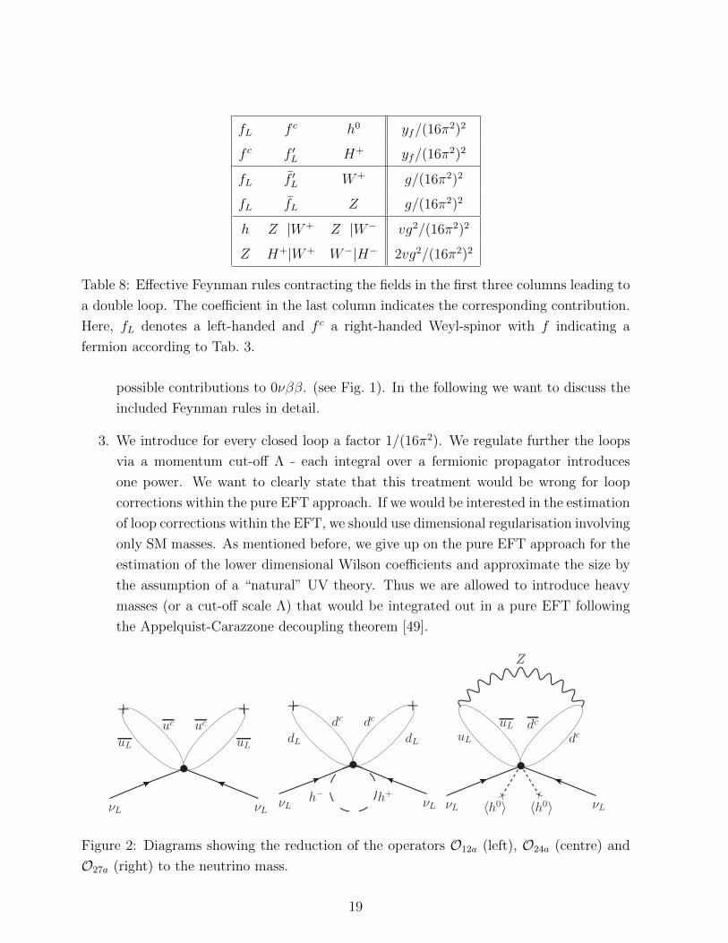
fL f c h0 yf/(16π2)2
f c f ′L H+ yf/(16π2)2
fL f ′L W+ g/(16π2)2
fL fL Z g/(16π2)2
h Z |W+ Z |W− vg2/(16π2)2
Z H+|W+ W−|H− 2vg2/(16π2)2
Table 8: Effective Feynman rules contracting the fields in the first three columns leading to
a double loop. The coefficient in the last column indicates the corresponding contribution.
Here, fL denotes a left-handed and f c a right-handed Weyl-spinor with f indicating a
fermion according to Tab. 3.
possible contributions to 0νββ. (see Fig. 1). In the following we want to discuss the
included Feynman rules in detail.
3. We introduce for every closed loop a factor 1/(16π2). We regulate further the loops
via a momentum cut-off Λ - each integral over a fermionic propagator introduces
one power. We want to clearly state that this treatment would be wrong for loop
corrections within the pure EFT approach. If we would be interested in the estimation
of loop corrections within the EFT, we should use dimensional regularisation involving
only SM masses. As mentioned before, we give up on the pure EFT approach for the
estimation of the lower dimensional Wilson coefficients and approximate the size by
the assumption of a “natural” UV theory. Thus we are allowed to introduce heavy
masses (or a cut-off scale Λ) that would be integrated out in a pure EFT following
the Appelquist-Carazzone decoupling theorem [49].
× ×
uL uL
uc uc
νL νL
× ×
dL dL
dcdc
h+h−νL νL νL νL
Z
××
dcdc
uL
uL
⟨h0⟩⟨h0⟩
Figure 2: Diagrams showing the reduction of the operators O12a (left), O24a (centre) and
O27a (right) to the neutrino mass.
19
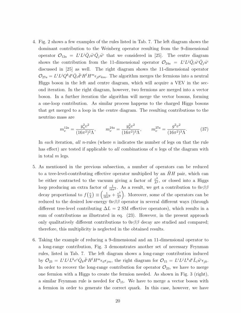
4. Fig. 2 shows a few examples of the rules listed in Tab. 7. The left diagram shows the
dominant contribution to the Weinberg operator resulting from the 9-dimensional
operator O12a = LiLjQiucQjuc that we considered in [25]. The centre diagram
shows the contribution from the 11-dimensional operator O24a = LiLjQiucQjuc
discussed in [25] as well. The right diagram shows the 11-dimensional operator
O27a = LiLjQkdcQidcHlHmεjlεkm. The algorithm merges the fermions into a neutral
Higgs boson in the left and centre diagram, which will acquire a VEV in the sec-
ond iteration. In the right diagram, however, two fermions are merged into a vector
boson. In a further iteration the algorithm will merge the vector bosons, forming
a one-loop contribution. As similar process happens to the charged Higgs bosons
that get merged to a loop in the centre diagram. The resulting contributions to the
neutrino mass are
m12aν =
y2uv
2
(16π2)2Λ, m24a
ν =y2dv
2
(16π2)3Λ, m27a
ν =g2v2
(16π2)3Λ. (37)
In each iteration, all n-rules (where n indicates the number of legs on that the rule
has effect) are tested if applicable to all combinations of n legs of the diagram with
in total m legs.
5. As mentioned in the previous subsection, a number of operators can be reduced
to a tree-level-contributing effective operator multiplied by an HH pair, which can
be either contracted to the vacuum giving a factor of v2
Λ2 , or closed into a Higgs
loop producing an extra factor of 116π2 . As a result, we get a contribution to 0νββ
decay proportional to f(vΛ
)≡(
116π2 + v2
Λ2
). Moreover, some of the operators can be
reduced to the desired low-energy 0νββ operator in several different ways (through
different tree-level contributing ∆L = 2 SM effective operators), which results in a
sum of contributions as illustrated in eq. (23). However, in the present approach
only qualitatively different contributions to 0νββ decay are studied and compared;
therefore, this multiplicity is neglected in the obtained results.
6. Taking the example of reducing a 9-dimensional and an 11-dimensional operator to
a long-range contribution, Fig. 3 demonstrates another set of necessary Feynman
rules, listed in Tab. 7. The left diagram shows a long-range contribution induced
by O23 = LiLjLkecQkdcHlHmεilεjm, the right diagram for O15 = LiLjLkdcLiucεjk.
In order to recover the long-range contribution for operator O23, we have to merge
one fermion with a Higgs to create the fermion needed. As shown in Fig. 3 (right),
a similar Feynman rule is needed for O15. We have to merge a vector boson with
a fermion in order to generate the correct quark. In this case, however, we have
20

νL eL⟨h0⟩×
dc
uL
dL
dc
h0
h+
⟨h0⟩
eL
ec
νL uL
Z
×
eL eL
eL dc
uc
Figure 3: Diagrams showing the reduction of the operators O23 (left) and O15 (right) to a
long-range 0νββ decay contribution.
νL νL××
ec
ec uLuL
dL
eL
Z
W
⟨h0⟩⟨h0⟩
Figure 4: Diagram showing the reduction of the operators O44c to the neutrino mass.
to additionally insert a Higgs VEV beforehand. In order to provide a converging
algorithm, the latter rule is added explicitly to the algorithm as indicated in Tab. 7.
We allow for up to three additional Higgs VEV insertions per diagram. This leads to
the following contributions
GF ε157√
2=
yexu g
2v
(16π2)2Λ3,
GF ε237√
2=ye(y
exd )2v2
(16π2)3Λ3, (38)
with ε157 = εS+P
S+P and ε237 = εS−PS+P .
7. Fig. 3 (left) shows another important feature. We need to distinguish between exter-
nal and internal Yukawa couplings. While the flavour of Yukawa couplings associated
with external fields is fixed to the first generation in order to generate 0νββ decay,
internal Yukawa couplings can be summed over all flavours (we assume per default
internal Yukawa couplings and indicate external Yukawa couplings, fixed to first gen-
eration with yex). This can make a significant impact in the discussion of the results,
as we will see later in more detail.
21
fR,L
f′L,R
fR f ′L
HfL
f′L
fL f ′L
W
×
fR,L
f′L,R
fL fR f ′L
H
×fR,L
f′L,R
fL fR f ′L
H
fR,L
f′L,R
fR f ′L
HfL
f′L
fL f ′L
W
×
fR,L
f′L,R
fL fR f ′L
H
×fR,L
f′L,R
fL fR f ′L
H
×fL
f′L
fR fL f ′L
W
×fL
f′L
fR fL f ′L
W
××fR,L
fL,R
f′R,L
fL fR f ′L
H
××fR
fL
f′L
fR fL f ′L
W
×fL
f′L
fR fL f ′L
W
×fL
f′L
fR fL f ′L
W
××fR,L
fL,R
f′R,L
fL fR f ′L
H
××fR
fL
f′L
fR fL f ′L
W
fR,L
f′L,R
fR f ′L
HfL
f′L
fL f ′L
W
×
fR,L
f′L,R
fL fR f ′L
H
×fR,L
f′L,R
fL fR f ′L
H
fR,L
f′L,R
fR f ′L
HfL
f′L
fL f ′L
W
×
fR,L
f′L,R
fL fR f ′L
H
×fR,L
f′L,R
fL fR f ′L
H
×fL
f′L
fR fL f ′L
W
×fL
f′L
fR fL f ′L
W
××fR,L
fL,R
f′R,L
fL fR f ′L
H
××fR
fL
f′L
fR fL f ′L
W
×fL
f′L
fR fL f ′L
W
×fL
f′L
fR fL f ′L
W
××fR,L
fL,R
f′R,L
fL fR f ′L
H
××fR
fL
f′L
fR fL f ′L
W
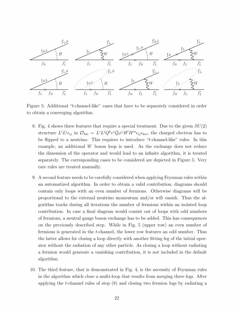
Figure 5: Additional “t-channel-like” cases that have to be separately considered in order
to obtain a converging algorithm.
8. Fig. 4 shows three features that require a special treatment. Due to the given SU(2)
structure LiLjεij in O44c = LiLjQkecQlecHlHmεijεkm, the charged electron has to
be flipped to a neutrino. This requires to introduce “t-channel-like” rules. In this
example, an additional W boson loop is used. As the exchange does not reduce
the dimension of the operator and would lead to an infinite algorithm, it is treated
separately. The corresponding cases to be considered are depicted in Figure 5. Very
rare rules are treated manually.
9. A second feature needs to be carefully considered when applying Feynman rules within
an automatized algorithm. In order to obtain a valid contribution, diagrams should
contain only loops with an even number of fermions. Otherwise diagrams will be
proportional to the external neutrino momentum and/or will vanish. Thus the al-
gorithm tracks during all iterations the number of fermions within an isolated loop
contribution. In case a final diagram would consist out of loops with odd numbers
of fermions, a neutral gauge boson exchange has to be added. This has consequences
on the previously described step. While in Fig. 5 (upper row) an even number of
fermions is generated in the t-channel, the lower row features an odd number. Thus
the latter allows for closing a loop directly with another fitting leg of the initial oper-
ator without the radiation of any other particle. As closing a loop without radiating
a fermion would generate a vanishing contribution, it is not included in the default
algorithm.
10. The third feature, that is demonstrated in Fig. 4, is the necessity of Feynman rules
in the algorithm which close a multi-loop that results from merging three legs. After
applying the t-channel rules of step (8) and closing two fermion legs by radiating a
22
Z boson, the remaining two fermions of the operator have to be connected with the
Z boson. The corresponding rules are listed in Tab. 8. Taking the example of O44c,
we obtain finally the following contribution:
m44cν =
g4v2
(16π2)4Λ. (39)
11. Given the described algorithm, each SU(2) decomposed operator is reduced to ev-
ery possible lower-dimensional or equal-dimensional operator via all possible loop
diagrams that can contribute to 0νββ decay. In a final step the most dominant
contribution is identified as described in the following.
We can compare our results for the mass mechanism with the result found in [46].
However, for certain operators discrepancies will occur (and are expected). Comparing
O29a with our results in Tab. 6, we obtain
m29a,1stν =
g2
(16π2)3
v2
Λ, (40)
while in [46] the contribution
m29a,3rdν =
y2u
(16π2)2
v2
Λf( v
Λ
)(41)
is found. This results from the determination of the dominant contribution. While Eq. 41
is dominant for third generation internal Yukawa couplings, Eq. (40) is the dominant one
for only first generation Yukawa couplings, cf. Fig. (6). As we store all contributions that
result from our algorithm, we are able to vary the generation of Yukawa couplings while
using the correct contribution of Eq. (41) and Eq. (40). The same behaviour occurs for
contributions of operators O74a, O74b and O75.
4.3 Determination of the Operator Scale
Having all the possible contributions of each operator, we need to identify the most domi-
nant ones. To do so we just simply compare their numerical values considering the values
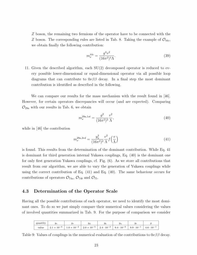
of involved quantities summarized in Tab. 9. For the purpose of comparison we consider
quantity ye yτ yd yb yu yt g
value 2.1× 10⁻⁶ 1.0× 10⁻² 2.0× 10⁻⁵ 2.4 · 10−2 9.4 · 10−6 9.9 · 10−1 4.6 · 10−1
Table 9: Values of couplings in the numerical evaluation of the contributions to 0νββ decay.
23

νL νL××
uL
uL uc
uc
Z
⟨h0⟩⟨h0⟩ νL νL××
uL
uc uL
uc
h0
⟨h0⟩⟨h0⟩ νL νL××
uL
uc uL
uc
× ×
⟨h0⟩⟨h0⟩
Figure 6: The dominant mass contribution of operator O29 for first generation internal
Yukawa couplings includes the gauge coupling (left) . For third generation internal Yukawa
couplings the corresponding contributions with Yukawa couplings are the dominant ones
(centre and right).
just first generation of fermions. As for the operator scale Λ, we assume its value to be
Λ = 2186 GeV, when doing the comparison. At this value, 116π2 = v2
Λ2 is roughly satisfied.
In other words, we assume such a value of Λ for which the suppression at one-loop corre-
sponds to the suppression by a factor v2
Λ2 . The reason is that for a number of operators one
gets a contribution involving an HH pair, which in the broken phase gives such a factor.
However, it can be at the same time closed into a trivial Higgs loop, thus contributing a
factor of 116π2 . As we want to keep both these contributions, we assume for convenience the
above stated value of Λ ensuring their equality.
We determine the dominant contribution to the light neutrino mass, the dominant
long-range contribution and the dominant short-range contribution separately. It is im-
portant to note that just these are then used for further calculations, which is, of course,
just an approximation. We do not sum over all possible contributions, and thus we do not
take into account the multiplicity (given e.g. by several different radiative reductions of
a specific operator to the same tree-level-contributing 0νββ decay operator) of any of the
contributions either. For each operator, the dominant contributions are listed in Tabs. 4, 5
and 6. The corresponding ε couplings excited by particular 0νββ decay contributions are
also shown therein. The relation to each coupling ε is made assuming a specific (convenient)
scalar Lorentz contraction (i.e. a simple Lorentz contraction not involving any γ matrices)
of the given operator. Considering other Lorentz structures of the initial operator different
ε couplings could be also triggered.
In 0νββ decay contributions listed in Tabs. 4, 5 and 6 the short-hand notation
f(vΛ
)≡(
116π2 + v2
Λ2
)is used and the numbers in brackets in front of several operators (in
the ‘Operator’ column) just notes the number of possible Lorentz or SU(3)c contractions
allowed for the given operator, appearing just when more than one such possibility exists.
24
Certain operators give several qualitatively different (but numerically similar) long-range
contributions that differ just by the involved Yukawa couplings. The possible flavours are
shown in a single subscript separated by vertical lines. The respective couplings ε excited
by given operators are also presented. For multiple long-range contributions we show mul-
tiple epsilons ordered accordingly with Yukawa coupling labels. Moreover, in some cases
one of the Yukawa flavour indices is shown in brackets, which means that the contribution
proportional to that particular type of Yukawa coupling includes only the factor v2
Λ2 and
not the loop factor 116π2 in f
(vΛ
). For example, the long-range contribution of operator 34
readingyexe|u|(d)
(16π2)2g2v
Λ3f(vΛ
)and the corresponding excited ε couplings εS+P
S+P |2εV+AV±A in fact stand
for 3 individual contributions yexe
(16π2)2g2v
Λ3f(vΛ
), yex
u
(16π2)2g2v
Λ3f(vΛ
)and
yexd
(16π2)2g2v3
Λ5 exciting ε-
couplings εS+PS+P , εV+A
V+A and εV+AV−A, respectively. Whenever a dash instead of a contribution is
shown, such a reduction of a particular operator is not possible in our approach and to be
able to obtain such a contribution one would have to consider what we call an ‘s-channel’
exchange rule, which is described in Section 6.3 in more detail.
Although all these contributions are presented, just the dominant one is used as in-
put in further calculations. For a given value of the 0νββ decay half-life, e.g. assuming a
hypothetical observation at a value of TXe1/2 = 1027 y, it is then easy to determine the corre-
sponding operator scale Λ that will be the basis to calculate the washout of lepton number
in the early Universe. In practice, we collect all contributions for a given operator, fix the
SM gauge and Yukawa couplings according to Tab. 9, possibly selecting between first and
third generation values for internal Yukawa couplings. We express the inverse 0νββ half-life
as a function of the operator scale Λ, defined as the maximum among all contributions.
We thus neglect any enhancement from two or more contributions of similar size but also
potential interference effects. The former will have little impact on the derived operator
scale; for the latter we would like to stress that we always assume (a currently hypothet-
ical) observation of 0νββ decay. If two or more contributions partially cancel each other,
it would in fact strengthen our argument as a given 0νββ measurement will correspond
to a stronger washout. Finally, assuming such a measurement, specifically TXe1/2 = 1027 y,
we determine the corresponding operator scale from the dominant contribution. As the
inverse half-life is ∝ Λ4−D, the dominant contribution corresponds to the highest scale of
the operator for a given half-life (if the scale were lower, the dominant contribution would
induce a more rapid 0νββ decay).
25
5 Lepton Number Washout
In this section, we study the washout effect of a pre-existing net lepton asymmetry from the
aforementioned operators. For simplicity, we assume only one LNV operator being active
at a time. The Boltzmann equation for a particle species N reads3
zHnγdηNdz
= −∑a,i,j,···
[Na · · · ↔ ij · · · ], (42)
where ηN is the number density of N normalized to the photon density, ηN ≡ nN/nγ, and
[Na · · · ↔ ij · · · ] =nNna · · ·neqNn
eqa · · ·
γeq(Na · · · → ij · · · )
− ninjneqi n
eqj · · ·
γeq (ij · · · → Na · · · ) . (43)
The space-time density of scattering in thermal equilibrium, γeq, with n initial particles
and m final particles is defined as
γeq(Na · · · → ij · · · ) =
∫d3pN
2EN(2π)3e−
ENT ×
∏a
[ ∫ d3pa2Ea(2π)3
e−EaT
]×∏i
[ ∫ d3pi2Ei(2π)3
]× (2π)4δ4
(pN +
∑a
pa −∑i
pi
)|M |2, (44)
with |M |2 being the squared amplitude summed over initial and final spins. As shown
in [52], by inserting unity into γeq,
1 =
∫d4Pδ4(P − pN −
∑pa)
=
∫1
2
√P 2
0 − s δ4(P − pN −∑
pa) ds dP0 dΩ, (45)
where s = P 20 − |~P |2 and Ω is the two-dimensional solid angle of the three-momentum ~P ,
the density of scatterings can be simplified as
γeq(Na · · · → ij · · · ) =1
2
1
(2π)4
∫ds
∫dΩ
∫dP0
√P 2
0
s− 1√s e−P0/T
×∫
d3pN2EN(2π)3
×∏a
[ ∫ d3pa2Ea(2π)3
](2π)4δ4(P − pN −
∑pa)
×∏i
[ ∫ d3pi2Ei(2π)3
](2π)4δ4(P −
∑pi)× |M |2
=1
2(2π)4
∫ds√s
∫dP0
√P 2
0
s− 1e−P0/T
∫dΩdPSndPSm × |M |2,
(46)
3See, for instance, Refs. [50–52] for more detailed discussions on the Boltzmann equation formalism.
26
in which∫
dPSn (∫
dPSm) is the initial (final) state phase space integral.
Assuming |M |2 does not depend on the relative motion of particles with respect to
the thermal plasma, one obtains after integrating over P0 and Ω,
γeq(Na · · · → ij · · · ) =1
(2π)3
∫ds√sK1
(√sT
)dPSndPSm × |M |2, (47)
withKn being the modified Bessel function of the second kind and∫
dΩ = 4π. Furthermore,
in case of all particles involved being scalars, |M |2 is simply proportional to (1/Λ2)N−4,
where Λ is the cut-off scale of the corresponding effective operator and N ≡ n+m. Since
|M |2 has no dependence on the phase space integral variables, γeq can be easily computed
in this case,
γeq =1
22(2π)2N−3× Γ(N − 2)Γ(N − 3)
Γ(n)Γ(n− 1)Γ(N − n)Γ(N − n− 1)× T 2N−4
Λ2N−8, (48)
where we use
PSn =
∫dPSn =
1
2(4π)2n−3
sn−2
Γ(n)Γ(n− 1), (49)
in the massless limit:√s mi (i = 1, · · · , N).
In case that a scalar is replaced by a fermion, the squared amplitude receives an ad-
ditional factor of E/Λ compared to the scalar-only case simply based on naive dimensional
analysis, where E has a dimension of energy and is determined by the details of interaction
kinematics. For interactions with a large number of particles involved, integration of |M |2over the phase space becomes quite complex in the presence of fermions. To obtain a good
approximation for integration, we replace E by (i) the centre-of-mass energy√s and by
(ii) the average energy√s/n (
√s/m) for an initial (final) state fermion, respectively. In
both cases, integration over the phase space integral is trivial as in the scalar case. Then,
we take the geometric mean of the results from the two replacements to be the final result
as described below.
To be more concrete, assuming there exist nf fermions within the n-particle initial
state and mf fermions within the m-particle final state4, the first method leads to |M1|2 =√sNf/2
ΛN−4+Nf/2
(Nf ≡ nf +mf ) while the second one results in |M2|2 = (√s/n)
nf/2(√s/m)
mf/2
ΛN−4+Nf/2
. As
a result, one obtains
γeq1(2)(Na · · · → ij · · · ) =
2Nf−2
(2π)2N−3× c1(2)
× Γ(N +Nf/2− 3)Γ(N +Nf/2− 2)
Γ(n)Γ(n− 1)Γ(N − n)Γ(N − n− 1)× T 2N+Nf−4
Λ2N+Nf−8, (50)
4The dimension of the effective operator, D, is correlated with the number of particles it contains –
N +Nf/2 = D.
27

with
c1 = 1 and c2 =1
nnf (N − n)Nf−nf, (51)
using these two approaches. Furthermore, one should include a symmetry factor to account
for identical particles in the initial and final state due to the phase space integral, and also
take into account the number of different ways for creation and annihilation, given the
identical particles. In addition, given an operator, there exist physically distinctive lepton
number washout processes by interchanging particles in the initial and final states. One
thus needs to sum up all contributions from each of the permutations. The final result for
the thermal rate γeq is estimated as
γeq =√
(Σγeq1 )× (Σγeq
2 ), (52)
where the summation symbol Σ indicates that the aforementioned permutations as well
as the symmetry factors have to be included. We have checked that the approximation
used here is in agreement with the true results up to 10% discrepancy for some of the
dimension-7 operators.
Equipped with the approximate formulae for γeq, we now compute the L washout
rate from the operator O8, LiecucdcHjεij5 chosen as an illustrative example. The operator
induces, for instance, the process Lec → ucdcH (treated as particles) while its complex
conjugate yields the inverse process Lec ← ucdcH. On the other hand, by a permutation
of the field operators, a physically different process ucdcH → Lec (ucdcH ← Lec) is also
created by O8 (O†8). The operator O8 can induce 3 ↔ 2 and 1 ↔ 4 processes, but the
1↔ 4 processes are suppressed in the phase space integral compared to those of 3↔ 2, as
can be seen from Eq. (49). Again, to compute the total L washout from O8, one should
sum over all the distinguishable permutations, thirty of them in total: twenty come from
(n,m) = (2, 3) and (3, 2), and ten arise from (n,m) = (1, 4) and (4, 1) where n (m) denotes
the number of the initial (final) state particles. Note that (2, 3) and (3, 2) correspond to
physically different processes; e.g. Lec ↔ ucdcH is not equivalent to ucdcH ↔ Lec.
Assuming that the SM Yukawa interactions and the sphalerons are in thermal equi-
librium, all relevant chemical potentials can be expressed in terms of the chemical potential
of the lepton doublet L` (` = e, µ, τ) [17]:
µH =4
21
∑`
µL` , µuc =5
63
∑`
µL` ,
µec` = µL` −4
21
∑`
µL` , µdc = −19
63
∑`
µL` . (53)
5All the fields should be regarded as the field operator. Wherever necessary, one has to be careful about
the distinction between the field operator and the particle.
28
The chemical potential is related to the normalized density η in the limit of |n− n| neq
as
n
neq=
η
ηeq≈ exp
(µT
)≈ 1 +
µ
T;
n
neq=
η
ηeq≈ 1− µ
T,
=⇒ η∆
ηeq≡ η − η
ηeq= 2
µ
T, (54)
where ηeq ≡ neq/neqγ = 1/2 (3/2 due to the color factor) for ec` (uc, dc) while ηeq = 1 for
the doublets L` and H. In light of the chemical potential dependence, one only needs to
compute the time evolution of the lepton doublet density since the densities of the other
particles can be inferred from ηL based on Eqs. (53) and (54). The Boltzmann equation of
Le reads6
zHnγd ηLed z
= −[Leec ↔ ucdcH
]+ (other permutations)
= −(nLenec
neqLeneqec− nucndcnHnequcn
eq
dcneq
H
)γeq(Leec → ucdcH) + · · ·
= −22µLe7T
γeq(Leec → ucdcH) + · · ·
= −11
7η∆Leγ
eq(Leec → ucdcH) + · · · , (55)
where we assumed first generation fermions and a universal chemical potential among three
lepton flavours. All possible permutations of 2 ↔ 3 and 1 ↔ 4 should be included. The
last two equalities come from Eqs. (53) and (54). One can obtain the Boltzmann equations
in a similar way for the antiparticle, Le. Finally, the thermal rate γeq can be computed
based on Eq. (52) and the total washout effect from the operator O8, LiecucdcHjεij is
zHnγdη∆Le
dz= −11
√195T 10
7π7Λ6η∆Le . (56)
In general, the washout effect from a dimension-D operator can be expressed as
zHnγdη∆Le
dz= −cD
T 2D−4
Λ2D−8D
η∆Le , (57)
where the equilibrium photon density is nγ ≈ 2T 3/π2 and the Hubble parameter is H ≈1.66√g∗ T 2/ΛPl (effective number of relativistic degrees of freedom: g∗ ≈ 107 in the SM,
Planck scale: ΛPl = 1.2 × 10¹⁹ GeV). The washout processes with an interaction rate ΓW
6If the operator being considered contains identical doublets (LL or HH), one should express the doublet
in terms of its components in order to obtain correctly the symmetry factor. In this case, ηeq = 1/2 (3/2)
for the (colored) SU(2)L doublet components.
29

can be regarded to be in equilibrium if
ΓWH≡ cDnγH
T 2D−4
Λ2D−8D
= c′DΛPl
ΛD
(T
ΛD
)2D−9
& 1, (58)
with c′D = π2cD/(3.3√g∗) ≈ 0.3 cD. It implies that the washout is effective within the
temperature interval
ΛD
(ΛD
c′DΛPl
) 12D−9
≡ λD . T . ΛD. (59)
The upper limit T . ΛD is imposed to ensure the validity of the effective operator approach,
but washout may continue above ΛD in an underlying UV theory as discussed in Section 7.
Furthermore, the lower bound on the scale of baryogenesis can be more precisely determined
by solving the Boltzmann equation, Eq. (57), from the baryogenesis scale down to the EW
scale to see if the observed baryon asymmetry can be reproduced. This leads to the lower
limit,
λD ≈[(2D − 9) ln
(10−2
ηobsB
)λ2D−9D + v2D−9
] 12D−9
, (60)
that is larger than λD obtained simply based on ΓW & H. We here conservatively assume
a primordial asymmetry of order one, perhaps generated in a non-thermal fashion.
One obvious question is the range of efficient washout of the 5D Weinberg operator.
It has been shown [22] that if neutrinos have Majorana masses, there exists an upper bound
on the scale of baryogenesis: T . 1012 GeV(1 eV/mν)2. That is because the underlying
lepton number violation mechanism which induces the Majorana masses will erase both
the lepton and baryon asymmetry with the help of the sphalerons. The same approach
was adopted in our previous work [26], where we instead use the current 0νββ constraints
on the effective neutrino mass mββ, leading to T . 2 × 10¹² GeV. As we shall see later,
the analysis of the washout effect based on the effective approach will not be valid above
the cut-off scales at which new particles can be produced on-shell. In the following, we in
any case focus on LNV operators other than the Weinberg operator, and correlate their
washout effect with the induced 0νββ rate.
6 Results
In our previous paper [25], we discussed the contribution of the four exemplary operators
O1,O8,O12a,O24a contributing at tree level to 0νββ decay as depicted in Fig. 1. In the
30
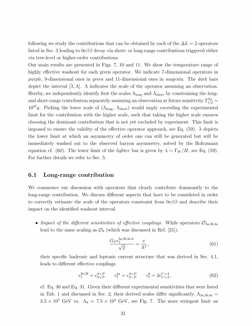
following we study the contributions that can be obtained by each of the ∆L = 2 operators
listed in Sec. 3 leading to 0νββ decay via short- or long-range contributions triggered either
via tree-level or higher-order contributions.
Our main results are presented in Figs. 7, 10 and 11. We show the temperature range of
highly effective washout for each given operator. We indicate 7-dimensional operators in
purple, 9-dimensional ones in green and 11-dimensional ones in magenta. The dark bars
depict the interval [λ,Λ]. Λ indicates the scale of the operator assuming an observation.
Hereby, we independently identify first the scales Λlong and Λshort by constraining the long-
and short-range contribution separately assuming an observation at future sensitivity TXe1/2 =
1027y. Picking the lower scale of (Λlong, Λshort) would imply exceeding the experimental
limit for the contribution with the higher scale, such that taking the higher scale ensures
choosing the dominant contribution that is not yet excluded by experiment. This limit is
imposed to ensure the validity of the effective operator approach, see Eq. (59). λ depicts
the lower limit at which an asymmetry of order one can still be generated but will be
immediately washed out to the observed baryon asymmetry, solved by the Boltzmann
equation cf. (60). The lower limit of the lighter bar is given by λ = ΓW/H, see Eq. (59).
For further details we refer to Sec. 5.
6.1 Long-range contribution
We commence our discussion with operators that clearly contribute dominantly to the
long-range contribution. We discuss different aspects that have to be considered in order
to correctly estimate the scale of the operators constraint from 0νββ and describe their
impact on the identified washout interval.
• Impact of the different sensitivities of effective couplings. While operators O3a,3b,4a
lead to the same scaling as O8 (which was discussed in Ref. [25]),
GF ε3a,3b,4a,87√
2=
v
Λ3, (61)
their specific hadronic and leptonic current structure that was derived in Sec. 4.1,
leads to different effective couplings
ε3a,3b7 = εS+PS+P ε4a7 = εS+P
S−P ε87 = 2εV+AV+A , (62)
cf. Eq. 30 and Eq. 31. Given their different experimental sensitivities that were listed
in Tab. 1 and discussed in Sec. 2, their derived scales differ significantly, Λ3a,3b,4a =
3.3 × 10⁵ GeV vs. Λ8 = 7.5 × 10⁴ GeV, see Fig. 7. The more stringent limit on
31

102
103
104
105
106
T[GeV
]
3a
3b
4a
4b
5 6
7
8
10
11a
11b
12a
12b
13
14a
14b
151617 18
19 20
24a
24b
25
26a
26b
27a
27b
28a
28b
28c
29a
29b30a
30b
31a
31b
32a
32b
3435
36 37 38
40a
43a
44c
76
EW scale
LHC reach
Figure 7: Temperature range of the effective washout for each given operator under the as-
sumption of an observation at future sensitivity of TXe1/2 = 1027y. We indicate 7-dimensional
operators in purple, 9-dimensional ones in green and 11-dimensional ones in magenta. The
darker part of the bar depicts the strong washout range between Λ and λ. The lower
limit of the lighter part is given by λ. Their definition is given in Eq. (59) and Eq. (60).
Both long-and short-range contributions to 0νββ decay induced by the operator under
consideration are taken into account. The orange diamond shows the scale of the Weinberg
operator. Orange arrows pointing up or down indicate a scale smaller or larger than the
range of the plot. All SM Yukawa couplings are chosen at their 1st generation values.
εS+PS+P = εS+P
S−P for O3a,3b,4a leads to a higher lower limit on the operator scale and
thus to a suppressed washout rate in comparison to O8. Under the assumption of
observing lepton number violation at the future sensitivity of TXe1/2 = 1027y, O8 would
exclude baryogenesis models above λ8 ≈ 900 GeV, while O3a,3b,4a can only exclude
models above λ3a,3b,4a ≈ 4 TeV.
• Impact of the SU(2) contraction on the lower washout bound. While the upper limit
Λ is the same for O3a,3b,4a, there is a small but crucial difference in the lower limit of
the strong washout regime, and thus on the scale above which baryogenesis can be
falsified, λ3a = 3.7 TeV and λ3b = λ4a = 4.6 TeV, cf. Fig. 7. This results from the
different SU(2) structure. As O3a contracts LiLiεij, it features fewer permutations
32

d
d u
e-
e-
GF
uO7
νL
h0
d
d u
e-
e-
GF
uO7
νL
h0
d
d u
e-
e-
GF
uO7
νL
h0 h0
h0
Figure 8: The 7-dimensional operators O3a,O3b ,O4a and O8 generate the long-range contri-
bution with one Higgs vev (left). The 9-dimensional operators O5,6 allow for both, closing
an Higgs loop and the insertion of Higgs vevs (centre and right), while the 9-dimensional
operator O8 allows only for Higgs mass insertions (right).
in the washout calculation (cf. Sec. 5) and thus a weaker washout rate than O3b or
O4a, leading to a higher lower limit on the washout interval.
As pointed out in [53] and mentioned in Sec. 3, O4b (and similarly O12b) has an
asymmetric lepton flavour structure and cannot induce 0νββ on its own. On the
other hand, it cannot be solely responsible for the observed neutrino oscillations
for the same reason. Minimally, there should thus be a misalignment between the
operator flavour structure and the charged-current mixing. Under this assertion,
these operators may still contribute to 0νββ with only O(1) suppression which is
why we retain them in our results.
• Impact of the specific field content. Naively one would expect that 9-dimensional
operators generate dominantly the short-range contribution at tree level. This is,
however, not necessarily case. O5, O6 and O7 featuring three Higgs doublets, con-
tribute dominantly to the long-range contribution with
GF ε5,67√2
=v
16π2Λ3+v3
Λ5and
GF ε77√
2=v3
Λ5, (63)
respectively. The different scaling arises from the different SU(2) structure. For
O5 = LiLjQkdcH lHmH iεjlεkm andO6 = LiLjQkucH lHkH iεjl, the Higgs doublets can
be additionally closed to a loop. The limit on their effective coupling is already that
strong such that Λ > 4πv, and the lower order contribution v/(16π2Λ3) dominates.
This is in contrast to O7 = LiQj ecQkHkH lHmεilεjm whose structure does not allow
for loop closing and thus scales with 1/Λ5, cf. Fig. 8. Generically, this leads to a
suppressed washout forO5, O6 andO7 in comparison to other 9-dimensional operators
and thus to a higher limit on the scale above which baryogenesis can be excluded, cf.
Fig. 7.
33

d
d
u
u
e-
e-
O9
d
d
u
u
e-
e-
O9
d
d u
e-
e-
GF
uO7
νL
h0
Figure 9: While O11a contributes only via one-loop at short range (left), O11b contributes
directly (centre). Both contribute by the same loop-suppression at long range (right).
6.2 Competition between long- and short-range contribution
For the above studied operators, it was straightforward to decipher which contribution
(long- vs. short-range) they generate dominantly. For other higher-dimensional operators
this is not necessarily the case. This is caused by the non-trivial interplay of different
aspects. Besides the ones we have discussed already, further have to be considered:
• Impact of the SU(2) structure on the dominant contribution. In order to demonstrate
the non-trivial interplay we compare the behaviour of O11a and O11a that differ only
in their SU(2) structure. While O11b contributes at tree level to the short-range
contribution, O11a contributes only one-loop suppressed, cf. Fig. 9,
G2F ε
11a9
2mp
=g2
16π2Λ5
G2F ε
11b9
2mp
=1
Λ5, (64)
with ε11a,b9 = ε1. The corresponding experimental limits are given in Tab. 1. Besides
their different short-range contributions, they contribute both identically to the long-
range contribution
GF ε11a,11b7√2
=ydv
16π2Λ3, (65)
with ε11a7 = ε11b
7 = εS+PS+P . As depicted in Fig. 9, O11a and O11b can be reduced
to O3a and O3b, respectively. We study the competition of long- and short range
contribution by comparing with Fig. 10 that shows the corresponding washout range
when constraining the operators’ contribution to long- (upper left panel) or short-
range (lower left panel) separately. As expected, O11b reproduces for the short-range
contribution the limits of O12a (discussed in Ref. [26]). The short-range contribution
of O11a, however, is loop suppressed, leading to a lower operator scale Λ11a9 and thus a
stronger washout than for O11b. Both operators contribute similarly to the long-range
34

102
103
104
105
106
T[GeV
]
3a
3b
4a
4b
5 6
7
8
10
11a
11b 12
a
12b
13
14a
14b
151617 18
1920
24a
24b
25
26a
26b
27a
27b
28a
28b
28c
29a
29b30a
30b
31a
31b
32a
32b
3435
37
40a
43a
44c
1st generation Yukawa couplingsLong-range contributions only
EW scale
LHC reach
102
103
104
105
106
T[GeV
]
3a
3b
4a
4b
5 6
7
8
10
11a
11b
12a
12b
13
14a
14b
15
16
17 18
19
20
21a
21b
23
24a
24b
25
26a 26
b
27a27b
28a
28b
28c
29a
29b
30a 30
b
31a31b
32a
32b
3435
37
40a
43a
44c
3rd generation Yukawa couplingsLong-range contributions only
EW scale
LHC reach
102
103
104
105
106
T[GeV
]
11a
11b
12a
14a
14b
19 20
24a
24b
28a
28b
28c
32a 36 37 38
76
1st generation Yukawa couplingsShort-range contributions only
EW scale
LHC reach
102
103
104
105
106
T[GeV
]
11a
11b
12a
14a
14b
19 20
24a
24b
28a
28b
28c
32a 36 37 38
76
3rd generation Yukawa couplingsShort-range contributions only
EW scale
LHC reach
Figure 10: Strong washout interval when constraining separately the operators’ long-range
(upper row) and short range contribution (lower row), both for first generation Yukawa
couplings only (first column) as well as for considering internal third generation Yukawa
couplings (second column). For further details on the legend see Fig. 7.
contribution leading to an operator scale Λ11a,b7 that is larger than Λ11a
9 but smaller
than Λ11b9 . This is summarized in Tab. 10 and reveals an interesting behaviour.
The naively expected behaviour is reproduced by O11b: The short-range contribution
dominates for the 9-dimensional operator,7 while the long-range contribution would
only dominate for scales Λ > 9894 GeV (for a detailed discussion how we derive the
limits on the operator scales, see Sec. 4.3. This is different for O11a: While it features
the same long-range contribution, the short-range contribution is loop suppressed
such that the long-range contribution dominates already above scales Λ > 472 GeV.
7As described in Sec. 4.3, we can always identify the higher scale with the more dominant contribution.
This can be understood as follows: we independently identify the scales Λlong and Λshort by constrain-
ing the long- and short-range contribution separately assuming an observation at the future sensitivity
TXe1/2 = 1027y. Picking the lower scale of (Λlong, Λshort) would imply exceeding the experimental limit for
the contribution with the higher scale, such that taking the higher scale ensures choosing the dominant
contribution that is not yet excluded by experiment. By comparing the upper row with the lower row of
Fig. 10, we can identify the dominant contribution. The corresponding scale is then taken to compile the
final comparison of washout regimes for different operators in Fig. 7 and Fig. 11.
35

O11a O11b
1st gen 3rd gen 1st gen 3rd gen
long-rangeT1/2
1.8×10⁻⁸
Λ60.01Λ6
1.8×10⁻⁸
Λ60.01Λ6
Λ 1623GeV 15501GeV 1623GeV 15501GeV
short-rangeT1/2
911Λ10
1.8×10⁸
Λ10
Λ 991GeV 3345GeV
dominant⋂
non-excluded long long short long
Table 10: For both operators we show T1/2(Λ) considering 1st generation Yukawa couplings
or internal 3rd generation Yukawa couplings. The corresponding operator scale is given
under the assumption of a future sensitivity of TXe1/2 = 1027y. We can identify the higher
scale with the dominant contribution that is not yet excluded by experiment, demonstrating
that the short-range contribution is dominant only for O11b with first generation Yukawa
couplings.
In other words, the loop suppression of the short-range contribution leads to the
dominance of the long-range contribution. This example demonstrates clearly that
the SU(2) contraction for the same operator can lead to significant changes in the
identification of the dominant contribution.
• Impact of the flavour structure on the dominant contribution. As 0νββ decay involves
only first generation quarks, we have assumed so far only first generation Yukawa cou-
plings in our calculations. However, comparing with Figs. 8, 9, Yukawa couplings in
loops are not necessarily fixed by external particles such that the final contribution
can be summed over loops including all flavours (democratic flavour structure). For
simplicity and a first comparison, we do not sum over all internal possibilities but re-
peat our analysis assuming internal third generation Yukawa couplings, while keeping
external first generation Yukawa couplings. The corresponding results are given in
Fig. 11. The results split in short- and long-range contributions are shown in Fig. 10
(right panels).
We want to study the effects again taking O11a and O11b as an example. While the
short-range contribution remains unchanged, the long-range contribution of O11b is
enhanced by the internal third generation coupling such that the long-range contribu-
tion dominates now already from scales Λ > 335 GeV on, cf. Fig. 10. This results in a
now dominant long-range contribution for O11b in contrast to a dominant short-range
contribution when considering only first generation Yukawa couplings, see as well
36

102
103
104
105
106
T[GeV
]
3a
3b
4a
4b
5 6
7
8
10
11a
11b
12a
12b
13
14a
14b
15
16
17 18
19
20
21a
21b
23
24a
24b
25
26a 26
b
27a27b
28a
28b
28c
29a
29b
30a 30
b
31a31b
32a
32b
3435
36 37 38
40a
43a
44c
76
EW scale
LHC reach
Figure 11: Same as Fig. 7, however internal SM Yukawa couplings are chosen at their 3rd
generation values, while external ones are kept at their 1st generation values.
Tab. 10. Due to the loop suppression of the short-range contribution, O11a features
already a comparably low scale above which the long-range contribution dominates
that is even more lowered when taking third generation Yukawa couplings into ac-
count (dominant long-range contribution for Λ > 16 GeV).
While already a change from an internal first to third generation down-type Yukawa
coupling leads to a swap in the dominant contribution, an even stronger effect is
expected for an internal up-type Yukawa coupling. This can be observed e.g. for O20
and its corresponding contributions
G2F ε
209
2mp
=1
Λ5,
GF ε207√
2=
yuv
16π2Λ3, (66)
with ε209 = 2ε5 and ε20
7 = 2εV+AV+A.
The examples discussed above clearly demonstrate that the long-range contribution
can dominate for 9-dim operators although one might naively expect that the short-
range contribution will be the most dominant one for these higher dimensional oper-
ators. The non-trivial interplay of scales is visualized for all operators in Fig. 10, and
the final results given in Fig. 7 and Fig. 11.
• Consequences for the washout and the experimental observation at colliders. Under
37
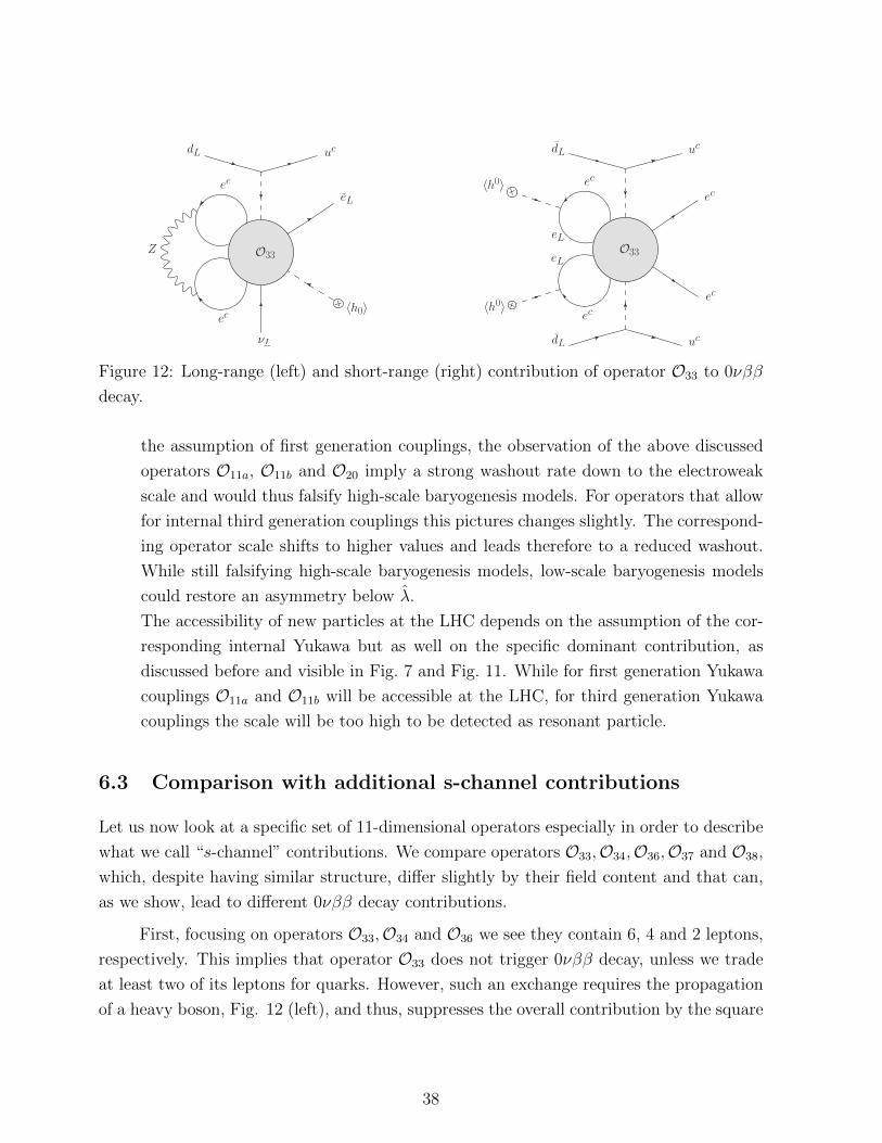
dL uc
〈h0〉
ec
ec
Z O33
νL
eL
dL uc
ec
ec
〈h0〉ec
〈h0〉
dL uc
ec
O33
eL
eL
Figure 12: Long-range (left) and short-range (right) contribution of operator O33 to 0νββ
decay.
the assumption of first generation couplings, the observation of the above discussed
operators O11a, O11b and O20 imply a strong washout rate down to the electroweak
scale and would thus falsify high-scale baryogenesis models. For operators that allow
for internal third generation couplings this pictures changes slightly. The correspond-
ing operator scale shifts to higher values and leads therefore to a reduced washout.
While still falsifying high-scale baryogenesis models, low-scale baryogenesis models
could restore an asymmetry below λ.
The accessibility of new particles at the LHC depends on the assumption of the cor-
responding internal Yukawa but as well on the specific dominant contribution, as
discussed before and visible in Fig. 7 and Fig. 11. While for first generation Yukawa
couplings O11a and O11b will be accessible at the LHC, for third generation Yukawa
couplings the scale will be too high to be detected as resonant particle.
6.3 Comparison with additional s-channel contributions
Let us now look at a specific set of 11-dimensional operators especially in order to describe
what we call “s-channel” contributions. We compare operators O33,O34,O36,O37 and O38,
which, despite having similar structure, differ slightly by their field content and that can,
as we show, lead to different 0νββ decay contributions.
First, focusing on operators O33,O34 and O36 we see they contain 6, 4 and 2 leptons,
respectively. This implies that operator O33 does not trigger 0νββ decay, unless we trade
at least two of its leptons for quarks. However, such an exchange requires the propagation
of a heavy boson, Fig. 12 (left), and thus, suppresses the overall contribution by the square
38

〈h0〉
〈h0〉
〈h0〉
dc
νL
eL
uL
ec
uLdc
ec h+
O36O36
dc
ec
uL
uL
ec
dc
〈h0〉
〈h0〉
Figure 13: Long-range (left) and short-range (right) contribution of operator O36 to 0νββ
decay.
of its mass and we get
OLR33 ∝yexd g
2v
(16π2)3Λ
1
m2H
. (67)
This kind of additional rule we call “s-channel”. As apparent from the Feynman diagram
shown above, the original 11-dimensional operator is first reduced to the Weinberg operator
and then a Yukawa interaction is attached to it. Therefore, it is obvious that this exotic
contribution to 0νββ decay will be subleading with respect to the standard mass mecha-
nism. While two quarks are enough for the long-range contribution, one needs four of them
for the short-range one. Therefore, two s-channel rules must be applied in that case, which
leads to a suppression by the fourth power of the Higgs mass, see Fig. 12 (right).
In general, when deriving the 0νββ decay contributions, we do not consider the s-
channel-type exchange rules. Consequently, for many operators in Tabs. 4, 5 and 6 the
short-range contribution is missing, as they do not have the right field content. There are
also operators (e.g. O2,O9) that do not give any long-range 0νββ decay contribution either
- such operators are omitted in the resulting Figs. 7, 10 and 11.
An example of the operator with no short-range contribution shown in Tab. 6 is O34.
It contains 4 leptons and 2 quarks and leads to a long-range 0νββ decay mechanism at
two-loop order without propagation of a heavy boson. On the other hand, for the short-
range contribution 2 more quarks are needed, and therefore, the s-channel rule must be
39
used again. Interestingly, in both cases one can reduce the operator to different long-range
mechanisms corresponding to distinct chiralities of the external particles, but the obtained
contribution factors have the same form and differ just in the type of the external Yukawa
coupling. Similarly, one can find more short-range contributions for each of these operators,
but the long-range contributions always dominate. In contrast to that, the operator O36
has the right field content, and thus, contributes to the short-range 0νββ decay mechanism
at tree level,
OSR36 ∝v2
Λ7, (68)
while at least two loops are needed in the long-range case,
OLR36 ∝yex2e ydv
(16π2)2Λ3
(1
16π2+v2
Λ2
), (69)
see Fig. 13. Moreover, the long-range contribution is further suppressed by external Yukawa
couplings; therefore, the leading contribution comes from the short-range mechanism. Since
the s-channel is not used, the contributions triggered by this operator are in general bigger
than contributions of operators O33 and O34. The operator O38 gives a very similar contri-
bution as operator O36. The only difference is that the internal Yukawa coupling appearing
in these three contributions is yu instead of yd.
An interesting behaviour can be observed in case of the operator O37. Analogous
to operators O36 and O38, it gives long-range contributions proportional to the second
power of the external Yukawa couplings, and thus, one would expect them to be similarly
suppressed. However, for O37 these contributions are not the dominant ones. There is
another long-range contribution containing a vector boson in the loop instead of the Higgs
(see Fig. 14), which makes it proportional to g2 times a single external Yukawa coupling,
OLR37 ∝yexe g
2v
(16π2)2Λ3
(1
16π2+v2
Λ2
). (70)
6.4 Comparison with the standard mass mechanism
As discussed in Sec. 2, we assumed in our analysis so far that 0νββ decay does not directly
originate from the Majorana neutrino mass mechanism but from another LNV new physics
contribution. Under this assumption, the 0νββ decay half life gives no direct informa-
tion about the neutrino mass although any LNV contribution will of course additionally
contribute to the Majorana mass. The corresponding washout interval was derived so far
40

〈h0〉 〈h0〉
〈h0〉 ec
ucdc
νL
W
dL uL
O37
Figure 14: Dominant long-range contribution of operator O37 to 0νββ decay.
under this assumption, neglecting the mass contribution for fixing the operator scale.
However, it is still interesting to consider the possibility that also the mass mechanism is
triggered only by loop contributions of the higher-dimensional operators in question. We
have thus derived as well the corresponding operator scale assuming the observation of
0νββ decay is generated by an underlying loop induced Weinberg-operator. We indicate
the corresponding scale with an orange diamond in Fig. 7 and Fig. 11. The orange arrows
pointing up or down indicate a scale smaller or larger than the range of the plot. Again, a
higher scale indicates the dominant contribution. A few comments are in order:
• 1st generation Yukawa couplings. Assuming only first generation Yukawa couplings,
long- or short-range contributions occur to be mainly dominant, cf. Fig. 7. Only for
around a fifth of the operators listed, the mass mechanism is dominant.
Naively one would expect that the mass mechanism dominates for the 7-dim operators
and 9-dim operators with 3 Higgs doublets (meaning up to O8) due to less loop
suppression than for higher operators. This is, however, not necessarily the case.
When an operator includes the SU(2) contraction LiLjεij, one lepton leg has to
be flipped, as discussed in Sec. 4.2 and additional loop factors suppress the scale.
The complementary structure LiLjεikεjl (or similar), however, is less suppressed.
To confront both cases, we refer to O3a and O3b as examples, cf. Fig. 15 and the
corresponding entries in Tab. 4. Whereas the long-range contribution dominates over
the mass mechanism for O3a, it is the opposite for O3b.
In contrast, higher-dimensional operators (9-dimensional and above), however, are
generally expected to be less constrained by the neutrino mass due to a higher order
loop suppression and small Yukawa couplings. As can be seen in Fig. 7, the mass
mechanism would mostly point to a far too small scale, demonstrating the need
of an additional mechanism to generate light neutrino masses. This would in turn
41
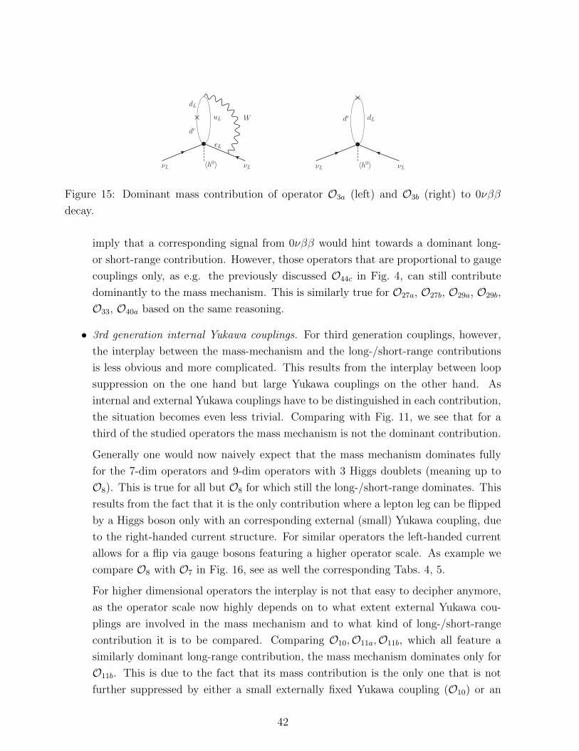
νL νL
W×dc
dL
uL
eL
⟨h0⟩ νL νL
×
dc dL
⟨h0⟩
Figure 15: Dominant mass contribution of operator O3a (left) and O3b (right) to 0νββ
decay.
imply that a corresponding signal from 0νββ would hint towards a dominant long-
or short-range contribution. However, those operators that are proportional to gauge
couplings only, as e.g. the previously discussed O44c in Fig. 4, can still contribute
dominantly to the mass mechanism. This is similarly true for O27a, O27b, O29a, O29b,
O33, O40a based on the same reasoning.
• 3rd generation internal Yukawa couplings. For third generation couplings, however,
the interplay between the mass-mechanism and the long-/short-range contributions
is less obvious and more complicated. This results from the interplay between loop
suppression on the one hand but large Yukawa couplings on the other hand. As
internal and external Yukawa couplings have to be distinguished in each contribution,
the situation becomes even less trivial. Comparing with Fig. 11, we see that for a
third of the studied operators the mass mechanism is not the dominant contribution.
Generally one would now naively expect that the mass mechanism dominates fully
for the 7-dim operators and 9-dim operators with 3 Higgs doublets (meaning up to
O8). This is true for all but O8 for which still the long-/short-range dominates. This
results from the fact that it is the only contribution where a lepton leg can be flipped
by a Higgs boson only with an corresponding external (small) Yukawa coupling, due
to the right-handed current structure. For similar operators the left-handed current
allows for a flip via gauge bosons featuring a higher operator scale. As example we
compare O8 with O7 in Fig. 16, see as well the corresponding Tabs. 4, 5.
For higher dimensional operators the interplay is not that easy to decipher anymore,
as the operator scale now highly depends on to what extent external Yukawa cou-
plings are involved in the mass mechanism and to what kind of long-/short-range
contribution it is to be compared. Comparing O10,O11a,O11b, which all feature a
similarly dominant long-range contribution, the mass mechanism dominates only for
O11b. This is due to the fact that its mass contribution is the only one that is not
further suppressed by either a small externally fixed Yukawa coupling (O10) or an
42

νL νL
WuL dL
×ec
eL
⟨h0⟩ νL νL
WuL dL
ec
eL
⟨h0⟩ νL νL
h+×dc
dL
uc
ec
⟨h0⟩
Figure 16: Dominant mass contributions to 0νββ decay generated from operatorO7 ∝ v2/Λ
(left), ∝ v4/Λ3 (centre) and the corresponding diagram for O8 (right).
νL νL
dL
dc dc
dL
uL
eL
× ×
W
νL νL
dL
dc dc
dL
× ×
Figure 17: Dominant mass contribution of operator O11a (left) and O11b (right) to 0νββ
decay.
additional loop suppression (O11a), cf. Fig. 17.
O16,O17,O18 demonstrate the opposite picture. While all feature the same mass con-
tribution, their dominant long-range contributions differ, cf. Fig. 18. While O17,O18
feature an additional loop suppression and an external Yukawa coupling, only O16
contributes directly. Thus, the non-standard contribution is still dominant for O16.
The 9-dim O19,O20,O76 and 11-dim O26a,b,O30a,b,O34,O35,O36,O37,O38 feature a
dominant non-standard contribution. This is mainly triggered by fixed external first
generation Yukawa couplings in the Weinberg contribution, suppressing the scale. For
a more detailed discussion about O34,O36,O37,O38, see Sec. 6.3.
While in Tabs. 4, 5 and 6, the dominant contribution is shown under the assumption of
first generation Yukawas only, we want to stress again that we have taken into account all
possibilities to generate the mass, long- and short-range contributions in our full analysis
shown in Fig. 7 to 11. Its importance can be demonstrated taking the example of O29a
and was already discussed in Sec. 4.2 in more detail. While Eq. (40) dominates only for
first generation Yukawa couplings, Eq. 41 is the dominant one when taking into account
third generation internal Yukawas, cf. Fig 6. This is especially interesting in the interplay
with similar operators as e.g. O29b that can generate only Eq. (40) due to its structure .
43

νL νL
ec
ec
dc
dL
uL
dL
uc
eL
Z
W
×
×
νL eL
uc
dc×
ec
ec
νL uL
Z
×
dc dc
eL dc
uc
Figure 18: Dominant mass contribution of operator O16 (left) that is similar for O17 and
O18 and the two different dominant long-range contributions of O16 (centre) and O17 (right)
to 0νββ decay.
7 Discussion and Conclusions
The observation of 0νββ decay, or LNV in general, would have profound consequences
for our understanding of nature. Specifically, it will likely lead us to an understanding
of the light neutrino masses and open a portal to new physics beyond the SM. The pres-
ence of LNV, or more generally B − L violating interactions, would also impact potential
mechanisms generating the observed baryon asymmetry of the universe. In this work, we
perform a detailed study on how effective SM invariant ∆L = 2 operators, which contain
the SM fermions and Higgs doublets, contribute to 0νββ decay both at tree and loop level.
In other words, we derive the effective scale Λ associated with the operator from a hypo-
thetical observation of 0νββ decay by considering the contributions an operator generates.
The ∆L = 2 operators of dimension-7, 9 and 11 are collected in Tabs. 4 - 6, adapted
from Ref. [46] and supplemented by the Hilbert Series method [48]. We mainly focus on
operators of dimension-7 and 9 but we also study a representative range of dimension-11 op-
erators, focusing on those that exhibit qualitatively different features from dim-9. Given an
operator, the tree-level contribution to 0νββ decay exists as long as the operator contains
the required particle content to realize the short-range or long-range interactions. To be
more precise, an operator that consists of two up- and two down-quarks as well as two elec-
trons, will have a short-range contribution. It is, however, highly non-trivial to manually
exhaust all possibilities of loop diagrams, stemming from the given operator, that trigger
0νββ decay. For example, the operator O16 includes the term νLeLdcececuc after SU(2)L
decomposition and thus has no short-range contribution at tree level. By connecting ec
and ec with an electron-mass insertion, the resulting lower-dimensional operator νLeLdcuc
triggers 0νββ via a long-range contribution.
To explore the large number of possibilities, and to discuss other observables in the
future, we have developed a tool which generates the radiative terms by closing loops,if nec-
44

uc
dc
WR
ec
L
HN
H
L
N
ec
WR
dc
uc
Figure 19: Two example diagrams in a left-right symmetric model framework that give rise
to the effective operator O8 = LiecucdcHjεij.
essary with mass insertions and Higgs/gauge boson emission. There is a rich phenomenol-
ogy involved in comparing the effect of different operators. Our results are summarized
in Tab. 4 -6, where the dominant long-range and short-range 0νββ contribution is given
for each operator, as well as with the associated neutrino mass scale generated radiatively
in the same fashion. The operator scale Λ is then shown in Fig. 7 and 11, corresponding
to a hypothetical observation of 0νββ decay at TXe1/2 = 1027 y and assuming the Yukawa
couplings involved are of first and third generation, respectively.
With the scale of a given ∆L = 2 operator determined from 0νββ decay, we compute
the corresponding washout rate on the lepton asymmetry in the early universe. We solve
the Boltzmann equation for the evolution of the lepton asymmetry in the presence of an
effective ∆L = 2 operator and the usual SM interactions, including sphaleron transitions.
All possible permutations of the particles, contained in the ∆L = 2 operator, corresponding
to physically distinctive washout processes, are taken into account. As a consequence, we
find a temperature range within which the washout is efficient and also infer a lower bound
on the temperature above which any pre-existing lepton or baryon asymmetry will be erased
by the operator.
The operator scale Λ and the associated temperature range of strong washout, given
an observation of 0νββ at T1/2 = 1027 y, can be as high as [λ,Λ] ≈ [2× 10³, 3× 10⁵] GeV
for dim-7 operators. These dim-7 operators, however, often have strong constraints from
the requirement to keep the neutrinos light. On the the other hand, dim-9 and dim-11
operators typically washout the lepton number in the range from 100 GeV to 1 TeV if the
underlying operator couples to first generation fermions only, in which case the constraint
from reproducing light neutrino masses can be evaded in many cases. Surprisingly, many
of the dim-9 and dim-11 operators in fact induce sizeable long-range contributions.
To better understand the washout from effective operators, we would like to comment
on the difference in terms of lepton number washout rates between the effective operator
45

-
[]
Γ/
Λ
( ν )=( -)
( )=( )
-
[]
Γ/
Λ
( ν )=( -)
( )=( )
Figure 20: Lepton number washout rate as a function of temperature from the UV processes
ucdc ↔ LecH (blue), LH ↔ ecucdc (red), and the sum of the two processes (purple)
computed based on the effective operator approach with the operator scale set to Λ =
7 × 10⁴ GeV. We show results for two different sets of values for the right-handed gauge
coupling gR and the neutrino Yukawa coupling yν . The corresponding heavy particle masses
are also shown.
approach and an underlying UV theory. For illustration, we choose the operator O8 =
LiecucdcHjεij and consider a left-right symmetric model (LRSM) [54–57], which gives rise
to this operator after integrating out the right-handed gauge boson WR and the right-
handed neutrino N . Moreover, instead of taking into account all permutations of the
initial and final state particles, we confine ourselves only to two of them to underscore the
impact of the resonant enhancement from on-shell WR or N . The two washout processes
of interest are ucdc ↔ LecH and LH ↔ ecucdc, respectively. The corresponding Feynman
diagrams in the LRSM are shown in Fig. 19. The computation of the scattering amplitudes
is straightforward and the thermal rate can be obtained based on Eq. (47). We also
calculate the washout rate for these two processes combined according to the effective
operator approach. The decay width of WR and N are estimated to be ΓWR= mWR
g2R/(8π)
and ΓN = mN(y2ν +
g4R
24π2m4N/m
4WR
)/(8π), respectively, where gR is the right-handed gauge
coupling and yν is the neutrino Yukawa coupling. In the limit of the momentum transferred
being much smaller than mWRand mN , the underlying UV theory and the effective operator
should produce the same result which can be ensured by requiring g2Ryν/(m
2WRmN) = 1/Λ3.
In Fig. 20, we show the normalised interaction rates with respect to the Hubble
expansion rate ΓW/H. The purple line indicates the washout rate of the effective operator
matched to the sum of the above two UV processes, while the blue and red line correspond
to the rate of the UV process ucdc ↔ LecH and LH ↔ ecucdc in Fig. 19, respectively. As
mentioned above, the couplings and masses in the LRSM are correlated with the effective
46

scale Λ, for which we use Λ = 7 × 10⁴ GeV taken from Fig. 7. For definiteness, we set
mWR= 1.5mN with two different sets of couplings: (gR, yν) = (1, 10−3) (left panel) and
(gR, yν) = (0.5, 10−3) (right panel). It is clear that with larger couplings, the masses mWR
and mN are also larger given the fixed operator scale Λ and so the resonance enhancement
occurs at higher temperatures. For small temperatures, the UV theory and the effective
operator yield consistent results as expected. For temperatures much larger than the masses
mWRand mN , the effective operator approach becomes unphysical while the real rate is
simply proportional to T . Moreover, the washout process becomes inefficient for much
higher temperatures since the Hubble expansion rate is proportional to T 2; the smaller gR
and yν , the lower the temperatures above which the L washout is out of equilibrium. All
in all, the lepton number washout remains, in principle, effective above the cut-off scale Λ,
and it can be even stronger than what is predicted by the effective operator approach due
to the resonance enhancement from new particles in an underlying UV theory. The details,
of course, are model-dependent. Our conclusion drawn based on the effective operator
approach that any pre-existing asymmetry above the scale λD will be erased, however, is
expected to hold since at low energies both the UV theory and effective operator should
yield the same result, unless the coupling constants in the UV theory are so small that the
new particles in the UV theory become very light and are below the EW scale.
It is worthwhile to point out that in case of LNV arising from the spontaneous break-
ing (for instance the triplet Higgs VEVs 〈∆L,R〉 breaking B − L in the LRSM), the cor-
responding symmetry is restored for temperatures above this breaking scale. In other
words, the L washout processes are expected to cease to work above the scale of symmetry
restoration.
We conclude the paper by commenting on a few limitations of our approach. First,
0νββ decay involves electrons but not µ and τ . To wipe out asymmetries stored in the
µ and τ flavours, one would also need to establish that those lepton flavour asymmetries
are equilibrated as well, e.g. by observing lepton flavour violation effective at the same
temperatures [26,58]. Second, to compute the washout effects in a model-independent way,
we simply assume that the baryon asymmetry generation mechanism is not related to the
washout process in question. It may be the case that the underlying L-violating theory
responsible for the washout also creates a lepton number asymmetry in the first place.
In other words, our conclusion only applies to those asymmetries generated before the L
washout becomes efficient. Finally, as pointed out in Ref. [59,60], if there exists a decoupled
sector which shares the baryon asymmetries with the visible sector, the L washout can not
completely erase all L asymmetries in the visible sector. That is because when the decoupled
sector communicated to the visible sector at very early times, it shared not only the baryon
47
asymmetry but also a hypercharge U(1)Y asymmetry. As the L washout processes preserve
the U(1)Y charge, the L asymmetry, which is proportional to U(1)Y asymmetry in this
case, can not be completely destroyed. After the sphalerons cease to work, the baryon
asymmetry in the decoupled sector can be converted back to the visible sector and thus
evade the washout process.
In any case, the observation of 0νββ will provide a means to test mechanisms of
baryogenesis in addition to mechanisms of neutrino mass generation. While the high-scale
seesaw mechanism operating at a scale of ≈ 1014 GeV remains a popular scenario, Majo-
rana neutrino mass mechanisms with an associated breaking of the lepton number close
to the EW scale are of strong theoretical interest. Such models generically predict new
contributions to 0νββ decay. To apply the reasoning put forward in our paper, it is nec-
essary to differentiate between different mechanisms responsible for 0νββ decay, at least
to distinguish exotic contributions from the standard neutrino mass mechanism. In the
context of 0νββ alone, this can be for example achieved by searching for 0νββ decay in
multiple isotopes [61–63] or by utilizing experiments that are sensitive to the individual
electron energies [64–68], for instance in the SuperNEMO experiment [69,70]. The presence
of non-standard contributions to 0νββ decay could also manifest as potential inconsisten-
cies between the results from 0νββ decay and from the determination of neutrino masses
from cosmological considerations [71]. More generally, LNV can also be probed in other
observables; for example, searches at high energy colliders for LNV in resonant processes
would have the advantage of pinpointing the LNV scale more directly as demonstrated
in [25,26].
Our results show that the scale Λ of many of the ∆L = 2 operators and the cor-
responding temperature range of strong washout are O(TeV) assuming an observation of
0νββ in future or planned experiments with a sensitivity of T1/2 ≈ 1027 y. In this case,
there is underlying new physics at work, potentially within the reach of the LHC and future
colliders. Together with the B + L-violating sphalerons, the presence of LNV can erase a
pre-existing baryon and lepton asymmetry generated at high temperatures. As a result, the
observation of 0νββ decay will strongly constrain models of high-scale (& TeV) scenarios
of baryogenesis and leptogenesis.
Acknowledgements
The authors are grateful to Martin Hirsch and Heinrich Pas for collaboration during the
early stages of this project. The authors would like to thank Brian Henning and Carlos
48

Tamarit for useful discussions on renormalisation in effective field theories and Marcela
Paz Gonzalez for useful discussions on the QCD running of neutrinoless double beta decay
operators. The work of FFD and LG was supported by an STFC Consolidated Grant
and a Royal Society Exchanges Grant. JH was supported by the Labex ILP (reference
ANR-10-LABX-63) part of the Idex SUPER, and received financial state aid managed by
the Agence Nationale de la Recherche, as part of the programme Investissements d’avenir
under the reference ANR-11-IDEX-0004-02. WCH was supported by DGF Grant No. PA
803/10-1 and by Danish Council for Independent Research Grant DFF-6108-00623.
References
[1] ATLAS Collaboration, G. Aad et al., Phys.Lett. B716, 1 (2012), 1207.7214.
[2] CMS Collaboration, S. Chatrchyan et al., Phys.Lett. B716, 30 (2012), 1207.7235.
[3] Particle Data Group, K. A. Olive et al., Chin.Phys. C38, 090001 (2014).
[4] Planck, P. A. R. Ade et al., Astron. Astrophys. 594, A13 (2016), 1502.01589.
[5] S. Weinberg, Phys.Rev.Lett. 43, 1566 (1979).
[6] P. Minkowski, Phys.Lett. B67, 421 (1977).
[7] R. N. Mohapatra and G. Senjanovic, Phys. Rev. Lett. 44, 912 (1980).
[8] T. Yanagida, Conf.Proc. C7902131, 95 (1979).
[9] M. Gell-Mann, P. Ramond, and R. Slansky, Conf.Proc. C790927, 315 (1979),
1306.4669.
[10] J. Schechter and J. W. F. Valle, Phys. Rev. D22, 2227 (1980).
[11] S. L. Adler, Phys.Rev. 177, 2426 (1969).
[12] J. S. Bell and R. Jackiw, Nuovo Cim. A60, 47 (1969).
[13] G. ’t Hooft, Phys.Rev.Lett. 37, 8 (1976).
[14] Planck Collaboration, P. A. R. Ade et al., Astron.Astrophys. 571, A16 (2014),
1303.5076.
[15] M. Fukugita and T. Yanagida, Phys. Lett. B174, 45 (1986).
49
[16] M. Fukugita and T. Yanagida, Phys.Rev. D42, 1285 (1990).
[17] J. A. Harvey and M. S. Turner, Phys. Rev. D42, 3344 (1990).
[18] B. A. Campbell, S. Davidson, J. R. Ellis, and K. A. Olive, Phys. Lett. B297, 118
(1992), hep-ph/9302221.
[19] B. A. Campbell, S. Davidson, J. R. Ellis, and K. A. Olive, Phys.Lett. B256, 484
(1991).
[20] B. A. Campbell, S. Davidson, J. R. Ellis, and K. A. Olive, Astropart.Phys. 1, 77
(1992).
[21] W. Fischler, G. Giudice, R. Leigh, and S. Paban, Phys.Lett. B258, 45 (1991).
[22] A. E. Nelson and S. M. Barr, Phys.Lett. B246, 141 (1990).
[23] V. A. Kuzmin, Pisma Zh. Eksp. Teor. Fiz. 12, 335 (1970).
[24] R. N. Mohapatra and R. E. Marshak, Phys. Rev. Lett. 44, 1316 (1980).
[25] F. F. Deppisch, J. Harz, and M. Hirsch, Phys.Rev.Lett. 112, 221601 (2014), 1312.4447.
[26] F. F. Deppisch, J. Harz, M. Hirsch, W.-C. Huang, and H. Pas, Phys. Rev. D92,
036005 (2015), 1503.04825.
[27] J. Harz, W.-C. Huang, and H. Pas, Int. J. Mod. Phys. A30, 1530045 (2015),
1505.07632, [Adv. Ser. Direct. High Energy Phys.25,207(2015)].
[28] J.-M. Frere, T. Hambye, and G. Vertongen, JHEP 0901, 051 (2009), 0806.0841.
[29] M. Dhuria, C. Hati, R. Rangarajan, and U. Sarkar, Phys. Rev. D92, 031701 (2015),
1503.07198.
[30] J. Schechter and J. Valle, Phys.Rev. D25, 2951 (1982).
[31] H. Pas, M. Hirsch, H. Klapdor-Kleingrothaus, and S. Kovalenko, Phys.Lett. B453,
194 (1999).
[32] H. Pas, M. Hirsch, H. Klapdor-Kleingrothaus, and S. Kovalenko, Phys.Lett. B498,
35 (2001), hep-ph/0008182.
[33] M. Agostini et al., (2017), 1703.00570, [Nature544,47(2017)].
50

[34] KamLAND-Zen, A. Gando et al., Phys. Rev. Lett. 117, 082503 (2016), 1605.02889,
[Addendum: Phys. Rev. Lett.117,no.10,109903(2016)].
[35] F. F. Deppisch, M. Hirsch, and H. Pas, J.Phys. G39, 124007 (2012), 1208.0727.
[36] M. Agostini, G. Benato, and J. Detwiler, Phys. Rev. D96, 053001 (2017), 1705.02996.
[37] nEXO, B. Mong, PoS HQL2016, 074 (2017).
[38] J. D. Vergados, H. Ejiri, and F. Simkovic, Int. J. Mod. Phys. E25, 1630007 (2016),
1612.02924.
[39] J. Engel and J. Menendez, (2016), 1610.06548.
[40] M. L. Graesser, JHEP 08, 099 (2017), 1606.04549.
[41] N. Mahajan, Phys. Rev. Lett. 112, 031804 (2014), 1310.1064.
[42] M. Gonzlez, M. Hirsch, and S. G. Kovalenko, Phys. Rev. D93, 013017 (2016),
1511.03945.
[43] C. Arbelaez, M. Gonzalez, S. Kovalenko, and M. Hirsch, (2016), 1611.06095.
[44] T. Peng, M. J. Ramsey-Musolf, and P. Winslow, Phys. Rev. D93, 093002 (2016),
1508.04444.
[45] V. Cirigliano, W. Dekens, M. Graesser, and E. Mereghetti, (2017), 1701.01443.
[46] A. de Gouvea and J. Jenkins, Phys.Rev. D77, 013008 (2008), 0708.1344.
[47] K. S. Babu and C. N. Leung, Nucl. Phys. B619, 667 (2001), hep-ph/0106054.
[48] B. Henning, X. Lu, T. Melia, and H. Murayama, JHEP 08, 016 (2017), 1512.03433.
[49] T. Appelquist and J. Carazzone, Phys. Rev. D11, 2856 (1975).
[50] K. Griest and D. Seckel, Phys. Rev. D43, 3191 (1991).
[51] J. Edsjo and P. Gondolo, Phys. Rev. D56, 1879 (1997), hep-ph/9704361.
[52] G. F. Giudice, A. Notari, M. Raidal, A. Riotto, and A. Strumia, Nucl. Phys. B685,
89 (2004), hep-ph/0310123.
[53] J. M. Berryman, de Gouvea Andre, K. J. Kelly, and A. Kobach, (2016), 1611.00032.
[54] R. N. Mohapatra and J. C. Pati, Phys.Rev. D11, 566 (1975).
51

[55] R. N. Mohapatra and J. C. Pati, Phys. Rev. D11, 2558 (1975).
[56] G. Senjanovic and R. N. Mohapatra, Phys.Rev. D12, 1502 (1975).
[57] R. N. Mohapatra and G. Senjanovic, Phys.Rev. D23, 165 (1981).
[58] L. Graf, J. Phys. Conf. Ser. 888, 012201 (2017).
[59] S. Dimopoulos and L. J. Hall, Phys. Lett. B207, 210 (1988).
[60] D. Aristizabal Sierra, C. S. Fong, E. Nardi, and E. Peinado, JCAP 1402, 013 (2014),
1309.4770.
[61] S. Bilenky and S. Petcov, (2004), hep-ph/0405237.
[62] F. Deppisch and H. Pas, Phys. Rev. Lett. 98, 232501 (2007), hep-ph/0612165.
[63] V. Gehman and S. Elliott, J.Phys.G G34, 667 (2007), hep-ph/0701099.
[64] M. Doi, T. Kotani, H. Nishiura, and E. Takasugi, Prog.Theor.Phys. 69, 602 (1983).
[65] M. Doi, T. Kotani, and E. Takasugi, Prog. Theor. Phys. Suppl. 83, 1 (1985).
[66] T. Tomoda, A. Faessler, K. Schmid, and F. Grummer, Nucl.Phys. A452, 591 (1986).
[67] A. Ali, A. Borisov, and D. Zhuridov, (2006), hep-ph/0606072.
[68] A. Ali, A. Borisov, and D. Zhuridov, Phys.Rev. D76, 093009 (2007), 0706.4165.
[69] F. Deppisch, C. Jackson, I. Nasteva, and S. Soldner-Rembold, Prog.Part.Nucl.Phys.
64, 278 (2010).
[70] SuperNEMO, R. Arnold et al., Eur. Phys. J. C70, 927 (2010), 1005.1241.
[71] F. Deppisch, H. Pas, and J. Suhonen, Phys. Rev. D72, 033012 (2005), hep-
ph/0409306.
52