Embed Size (px)
Citation preview
Do the opportunity costs of providing crop diversity differ between organic and conventional
farms? The case of Finnish agriculture
Anni Huhtala1 and Timo Sipiläinen
2
1MTT Agrifood Research Finland, Latokartanonkaari 9, FI-00790 Helsinki, Finland
2Department of Economics and Management, Box 28, FI-00014 University of Helsinki, Finland
Abstract
The attractiveness of targeted environmental policies on farmlands depends crucially on the
opportunity costs of the conservation programs. We use a crop diversity index as an indicator of
environmental output to compare the efficiency of conventional and organic crop farms. Technical
efficiency scores are estimated by applying data envelopment analysis to a sample of Finnish farms
for the period 1994 – 2002. We also estimate shadow values, or the opportunity costs, of producing
crop diversity. Our results show that there is variation in the shadow values between farms and the
technology adopted. The findings provide a basis for designing cost-effective policy instruments
such as auctions for conservation payments.
JEL Classification: C21, D24, H41, Q12, Q24
Keywords: biodiversity, Shannon index, DEA, technical efficiency, shadow values
1
1. Introduction
Biodiversity conservation on farmland is increasingly recognized as an important environmental
goal in agricultural policies (see Wossink and van Wenum, 2003; van Wenum et al., 2004). Yet,
agri-environmental policies are largely seen by the general public as subsidy programs that
compensate farmers for the costs of conservation measures but have not provided convincing
evidence of achieving a better environment. (Feng 2007) One of the challenges to be addressed in
designing environmental policies is measuring the benefits of environmental improvements. An
additional concern is that, due to asymmetric information, the costs of conservation on farmland are
not necessarily known by the regulator. (Sheriff 2009).
Calls have been heard for better incentives and market-like mechanisms for conservation - such as
auctions – to improve the effectiveness and impacts of policies designed to enhance biodiversity in
agriculture (e.g., Pascual and Perrings, 2007). The US Department of Agriculture has the longest
experience with auctions through its Conservation Reserve Program, in which farms are accepted
using an environmental benefits index (Latacz-Lohman & Van der Hamsvoort 1997, Kirwan et al.
2005). In contrast, European Common Agricultural Policy has mainly focused on dictating
appropriate farming practices instead of providing incentives for creating actual environmental
benefits. This orientation may be changing; there is growing interest in using auctions for delivering
payments for environmental services in agriculture (for a review see, e.g., Latacz-Lohman and
Schilizzi 2005). However, given the limited use of auctions in European agriculture, the bulk of the
research evaluating such policy instruments is based on pilot studies or experiments and simulations
carried out to test auction theory in alternative settings (see, e.g., Bastian et al. 2008, Glebe 2008,
Groth 2009). Given the hypothetical setting, the bids in experimental auctions do not necessarily
reflect farmers’ opportunity costs of conservation.
2
Our contribution is to analyze agricultural production within the frame of economic theory by
taking into account crop diversity as a positive non-market output of farms. The rationale here is
that if environmental goals are truly part of agricultural policies, it should be possible to evaluate
the performance of the policies implemented. As scarcity of resources is a point of departure for
economic analysis, the trade-offs in production of market and non-market outputs should be made
explicit. The opportunity costs of conservation measures ultimately determine the costs of the agri-
environmental policies implemented. To gain insight into the costs, we apply the framework
provided by Färe and Grosskopf (1998) to estimate shadow values for non-market public goods
such as environmental amenities. Variants of estimation methods within this framework have been
used to price negative externalities or public bads in European agriculture (e.g., Huhtala and
Marklund 2008, Piot-Lepetit and Le Moing 2007, Piot-Lepetit and Vermersch 1998). Less work has
been carried out on pricing the effects of agriculture on biodiversity conservation; the closest
analysis of biodiversity related to ours is an application by Färe et al. (2001) pricing the non-market
characteristics of conservation land in the United States.
In our analysis, we use crop diversity as a non-market output measured by a farm-level Shannon
diversity index capturing both the richness and evenness of cultivated crops on the farms. The index
is a typical landscape diversity indicator which can be seen as reflecting the esthetic value of a
diverse agricultural landscape from a social point of view. On the other hand, in the literature on
risk management in agriculture, crop diversity has been attributed a private value as an option for
risk-averse farmers to hedge against uncertainty (for a discussion see, e.g., Di Falco and Perrings
2005). On these grounds, the trade-off between market output (crop yield) and non-market
ecological by-product (crop diversity) can be considered relevant for farmers’ decision making.
3
Finally, it is important to bring out how the European agricultural policies that have been
implemented have become manifested in choices of farming practices and the corresponding
(ecological) benefits. Organic production can be seen as a more restricted technology which has
been promoted for environmental reasons1. We estimate the performance of conventional and
organic crop farms – two alternatives technologically - to evaluate their efficiency in using scarce
resources in the production of both crop yield and crop diversity. This comparison sheds light on
the impact of including crop diversity on the economic and environmental performance of the
farms. Moreover, we estimate the opportunity costs of crop diversity in terms of crop output
forgone. This information is important for policy design since it reveals whether there is
heterogeneity in the costs between types of farms and room for improving the cost-efficiency of
policies targeting the conservation of crop biodiversity in agriculture.
The paper is organized as follows. In section 2 we introduce and discuss the crop biodiversity index
applied in the empirical study. In section 3 we elaborate the fundamental approaches of the study in
terms of production economics: we present models of technical efficiency when there are multiple
outputs and, alternatively, when one of the outputs is held as a minimum constraint, and we derive
shadow values for crop diversity using these two alternative models. Section 4 presents how non-
parametric technical efficiency scores are estimated by applying data envelopment analysis (DEA).
Section 5 presents the annual data for the period 1994 – 2002 obtained from cross sections of
Finnish crop farms participating in the EU’s FADN bookkeeping system. As the number of organic
farms is small, the technique known as window analysis (Charnes et al. 1985) is applied to the
1 Organic farming as a method of production puts high emphasis on environmental protection. It avoids, or substantially
reduces, the use of synthetic chemical inputs such as fertilizers, pesticides and additives. Crop production makes use of
fertilization with manure, growing legumes to bind nitrogen from the air, composting of vegetables of low-soluble
fertilizers, and preventive measures to control pests and diseases. Crop rotation, mechanical weed control and the
protection of beneficial organisms are also important (Organic Farming in the EU: Facts and Figures, 2005). These
restrictions most likely have an impact on the production technology and economic performance of organic farms.
4
sample of organic farms when estimating efficiency scores with an assumption of progressive
technical change in four-year periods. The empirical results are reported in section 6. The
concluding section takes up a finding on variation in the shadow values between farms and between
the technologies adopted.
2. Crop biodiversity
In agricultural systems, biodiversity may be produced as a positive by-product in addition to
marketable output such as cereals. Management practices may have various impacts on biodiversity
due to crop rotation, application of chemical inputs and similar choices by the farmer. Biodiversity
is a complex concept with several dimensions and choosing proper measures or indicators for it
poses a challenge. The availability of data is a major limitation for empirical analysis. Here, we rely
on a relatively simple measure of diversity known as the crop diversity index, which can be
described as a measure of landscape diversity. According to a classification by Callicott et al.
(1999), the crop diversity index belongs to compositional measures of species diversity.
Species-level diversity is quantified as the number of species in a given area (richness) and how
evenly balanced the abundances of each species are (evenness) (Armsworth et al., 2004). It should
be noted that species-level biodiversity is only one of the measures that can be used in analyzing
biodiversity. For example, community level biodiversity describes species interactions in their
natural habitats. The spatial scale is also important since richness increases with area. Usually the
choice is either an economically or an ecologically meaningful scale. We choose to study the
diversity of agricultural land use at the farm level within the framework of production theory. At the
farm level, we know the number of crops cultivated and the area under each crop. When discussing
the mechanisms causing increased homogeneity of agricultural habitats, Benton et al. (2003) point
5
out that a reduction in the botanical and structural variety of crops and grassland grown on a single
farm increases the probability of larger blocks of land being under the same management at any
given time. Moreover, Jackson et al. (2007) identify valuation of biodiversity in agricultural
landscapes from socioeconomic perspectives as a critical issue requiring scientific research. For
these purposes, crop diversity is an appealing measure for analyzing the trade-offs and synergies
involved in managing for agricultural productivity as opposed to biodiversity conservation. In
addition, farm-level data are already available for use by government authorities for implementing
policy based on crop diversity indices. In fact, cultivation of local crops has been included as a
voluntary conservation measure eligible for specific support in the Finnish agri-environmental
program, but it has not gained wide popularity among farmers. (Horisontaalinen maatalouden
kehittämisohjelma 2006)
In this study, richness is measured by the number of cultivated crops, such as barley, grass silage,
potato, or areas lying fallow. Evenness refers to how uniformly the arable land area of a farm is
distributed among these different crops and uses. Evenness and richness, which describe diversity,
can be quantified using the Shannon diversity index (SHDI) (Armsworth et al., 2004). The index,
which has its origin in information theory (Shannon 1948), has been applied in a number of
environmental economic studies (e.g., Pacini et al., 2003; Hietala-Koivu et al., 2004; Latacz-
Lohman, 2004; Miettinen et al., 2004; Di Falco and Perrings, 2005).
The SHDI is calculated using the following formula:
)ln(1
i
J
i
i PPSHDI ×−= ∑=
, (1)
6
where J is the number of cultivated crops, Pi denotes the proportion of the area covered by a
specific crop and ln is the natural logarithm.2 The index in equation (1) equals zero when there is
only one crop, indicating no diversity. The value increases with the number of cultivated crops and
when the cultivated areas under various crops become more even. The index reaches its maximum
when crops are cultivated in equal shares, that is, when Pi =1/J (McGarical and Marks 1995).
In our analysis, the index is used to approximate the diversity produced by farms, and is therefore
modeled as a good output within the frame of production theory. Crop diversity has usually been
applied as a landscape indicator at the regional level. However, the use of crop diversity at the farm
level as well can be motivated by the fact that the number of different habitats is likely to increase
with crop diversity. In conventional farming, a monoculture may be successful, whereas organic
production technology requires at least some crop rotation, ruling out the possibility of a
monoculture. Thus, organic farming is likely to produce higher crop diversity. Numerous studies
have also shown that crop rotation conserves soil fertility (Riedell et al., 1998; Watson et al., 2002),
improves nutrient and water use (Karlen et al., 1994) and increases yield sustainability (Struik and
Bonciarelli, 1997; see also Herzog et al., 2006).
3. Production Technology
3.1 Description of technology
Input and output distance functions can be used to describe the technology when only input and
output quantities are known (Shephard, 1953; 1970). In contrast to the traditional scalar-valued
2 The Shannon diversity index appears in the literature under the name the Shannon-Wiener (-Weiner or –Weaver)
index. According to Keylock (2005), it belongs to the Hill family of indices (like the Simpson diversity index) and is
based on the Bolzmann-Gibbs-Shannon entropic form. Sometimes the index is presented in the form exp(SHDI). At the
maximum this form indicates the number of species corresponding to a uniform distribution (maximum entropy).
7
production function, distance functions allow multiple outputs (and multiple inputs). For any (x,y)
∈ R+M+N
the output distance function Do(x,y) is such that
Do(x,y) = min {λ > 0: y/λ ∈ P(x)}. (2)
The output distance function calculates the largest expansion from 0 of y along the ray through y
while staying in the producible output set (P(x)), which means that y belongs to P(x) if and only if
Do(x,y) ≤ 1. The distance function takes the value 1 only if the output vector belongs to the frontier
of the corresponding input vector. The output distance function thus completely characterizes the
technology, because it inherits its properties from P(x).
Probably the most frequently used models of technical efficiency are variants of the Farrell type
model.3 The Farrell (1957) measure of output-oriented technical efficiency is the reciprocal of the
output distance function, i.e. Fo(x,y) = (Do(x,y))-1. Thus
Fo(x,y) = max {µ: µy∈ P(x)}. (3)
By duality, output and input orientations have a convenient interpretation as an increase in revenue
and a reduction in costs, respectively. One of the attractive properties of a Farrell measure is that it
is invariant with respect to the units of measurement used for inputs and outputs.
3 Chambers et al. (1998) have shown that the proportional distance function (the reciprocal of Farrell technical
efficiency) is a special case of directional distance functions.
8
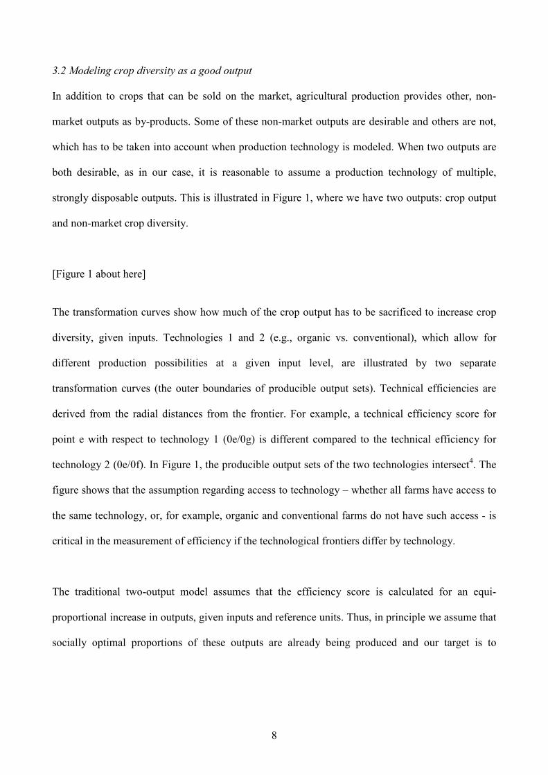
3.2 Modeling crop diversity as a good output
In addition to crops that can be sold on the market, agricultural production provides other, non-
market outputs as by-products. Some of these non-market outputs are desirable and others are not,
which has to be taken into account when production technology is modeled. When two outputs are
both desirable, as in our case, it is reasonable to assume a production technology of multiple,
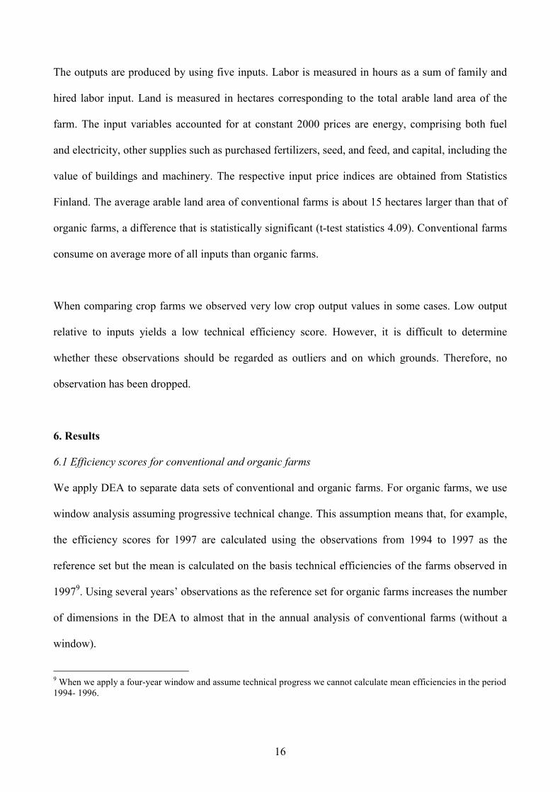
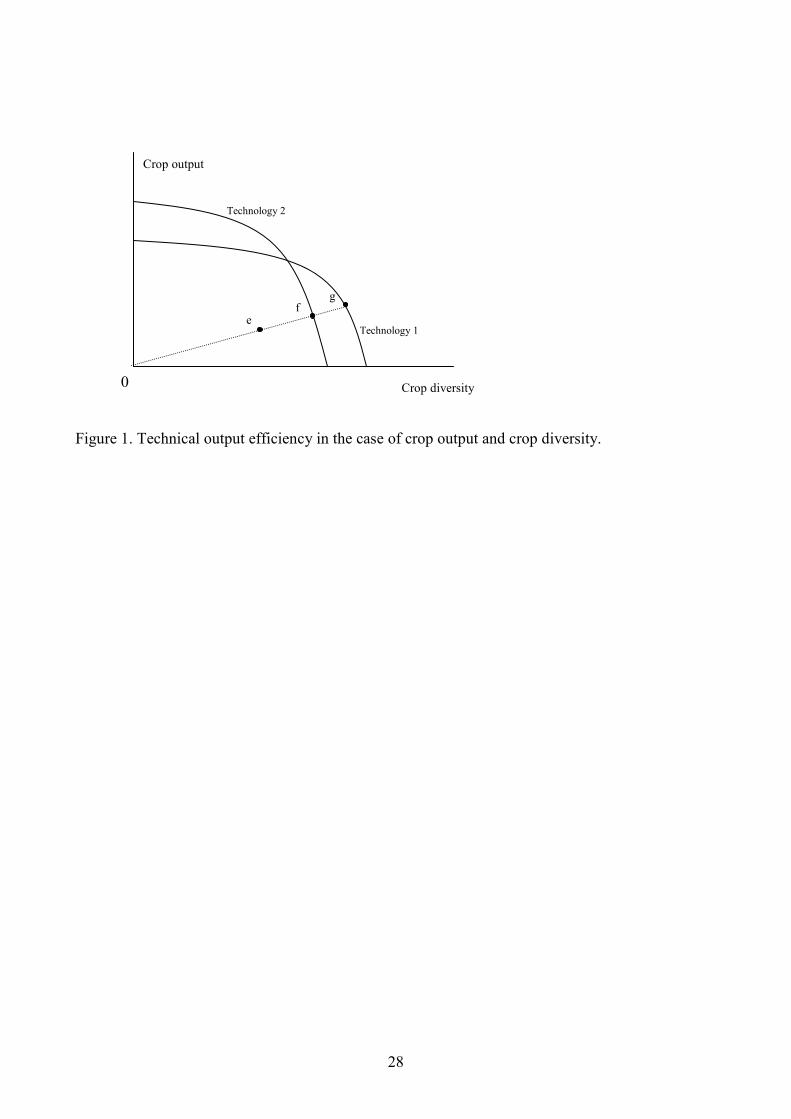
strongly disposable outputs. This is illustrated in Figure 1, where we have two outputs: crop output
and non-market crop diversity.
[Figure 1 about here]
The transformation curves show how much of the crop output has to be sacrificed to increase crop
diversity, given inputs. Technologies 1 and 2 (e.g., organic vs. conventional), which allow for
different production possibilities at a given input level, are illustrated by two separate
transformation curves (the outer boundaries of producible output sets). Technical efficiencies are
derived from the radial distances from the frontier. For example, a technical efficiency score for
point e with respect to technology 1 (0e/0g) is different compared to the technical efficiency for
technology 2 (0e/0f). In Figure 1, the producible output sets of the two technologies intersect4. The
figure shows that the assumption regarding access to technology – whether all farms have access to
the same technology, or, for example, organic and conventional farms do not have such access - is
critical in the measurement of efficiency if the technological frontiers differ by technology.
The traditional two-output model assumes that the efficiency score is calculated for an equi-
proportional increase in outputs, given inputs and reference units. Thus, in principle we assume that
socially optimal proportions of these outputs are already being produced and our target is to
9
produce more of both. This is a critical assumption when we take into account non-market outputs,
which by definition do not have a market price. We may also think that society’s aim is to increase
either crop diversity given the inputs and traditional output, or the traditional crop output given the
inputs and crop diversity. This can be interpreted to mean that a socially optimal level of one of the
outputs is already being produced but society seeks to evaluate the possibilities to increase the other
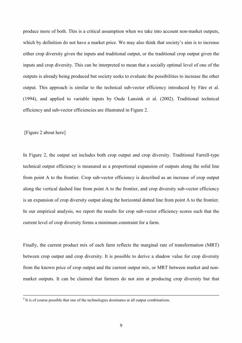
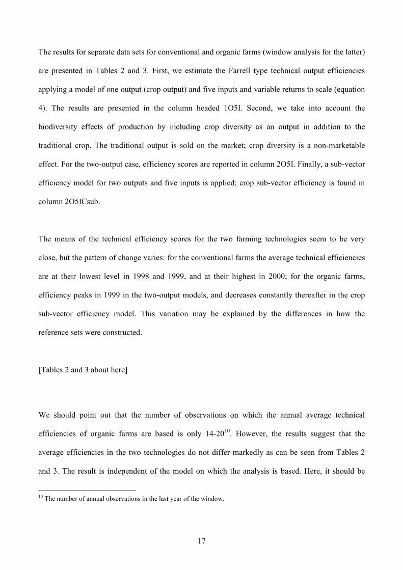
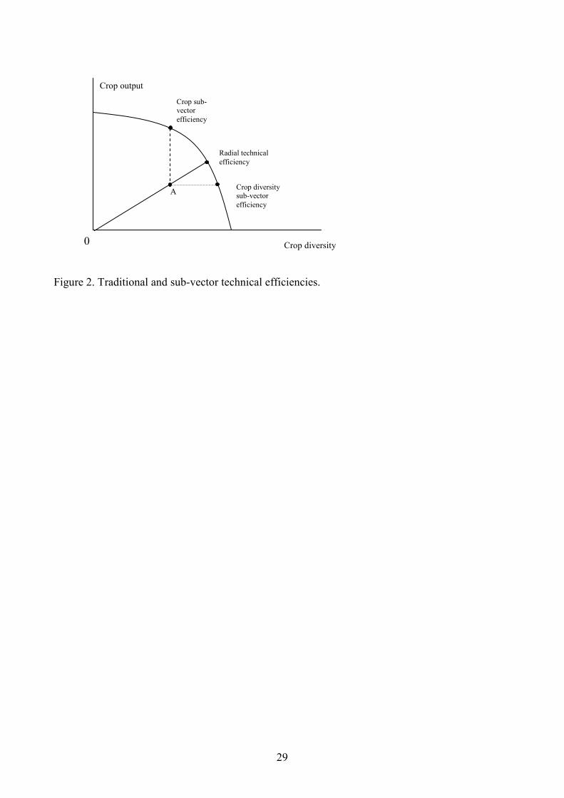
output. This approach is similar to the technical sub-vector efficiency introduced by Färe et al.
(1994), and applied to variable inputs by Oude Lansink et al. (2002). Traditional technical
efficiency and sub-vector efficiencies are illustrated in Figure 2.
[Figure 2 about here]
In Figure 2, the output set includes both crop output and crop diversity. Traditional Farrell-type
technical output efficiency is measured as a proportional expansion of outputs along the solid line
from point A to the frontier. Crop sub-vector efficiency is described as an increase of crop output
along the vertical dashed line from point A to the frontier, and crop diversity sub-vector efficiency
is an expansion of crop diversity output along the horizontal dotted line from point A to the frontier.
In our empirical analysis, we report the results for crop sub-vector efficiency scores such that the
current level of crop diversity forms a minimum constraint for a farm.
Finally, the current product mix of each farm reflects the marginal rate of transformation (MRT)
between crop output and crop diversity. It is possible to derive a shadow value for crop diversity
from the known price of crop output and the current output mix, or MRT between market and non-
market outputs. It can be claimed that farmers do not aim at producing crop diversity but that
4 It is of course possible that one of the technologies dominates at all output combinations.
10
diversity is a by-product of the production process. However, there may be differences between
farms in their location on the transformation curve (different shadow values) because of unobserved
heterogeneity in resources or heterogeneous risk preferences. This variation provides an opportunity
to target policy actions such that they contribute to crop diversity.
4. Estimation
4.1 Data envelopment models
A firm is said to be technically efficient if it lies on the boundary of the output possibility set, )(xP .
There are several ways to define this boundary. Data envelopment analysis (DEA) is a non-
parametric method that provides a piecewise linear, convex or non-convex envelopment for a set of
observations. The method has been developed for evaluating the performance of multi-input/multi-
output production (see Debreu, 1951; Farrell, 1957 and Koopmans, 1951; Charnes et al., 1978).
The DEA models applied in this study are output oriented and assume that P(x) satisfies convexity
and free disposability. If technical efficiency obtains its maximal value (one), the production is
efficient, and it is not possible to increase output with the given inputs in comparison to the
reference units. If production is technically inefficient, output can be increased using the given
inputs.
DEA models are fairly simple linear programming (LP) models which have to be solved for each
decision-making unit (farm) separately. In the case of variable returns to scale, we define the model
with outputs, ym, and inputs, xn, and k decision-making units forming the reference set and each
unit, k’, compared in turn to the set. In our notation below, ( , )oF VRS S , or φ , denotes technical
output efficiency under assumptions of variable returns to scale (VRS) and strong disposability (S).
11
The efficiency measure is the reciprocal of the output distance function, 1( ( , ))oD x y − (Färe et al.,
1994). The superscript t in Equation (5) refers to the annual solution of the LP problem.
1
'
1
'
1
1
( , ) ( ( , )) max
. . , 1,..., ,
, 1,... ,
1,
0, 1,..., .
t
o o
Kt t
k m k km
k
Kt t
k kn k n
k
K
k
k
k
F VRS S D x y
s t y z y m M
z x x n N
z
z k K
φ
φ
−
=
=
=
= =
≤ =
≤ =
=
≥ =
∑
∑
∑
(4)
The DEA model of variable returns to scale is obtained by including a constraint for intensity
variables 1kz =∑ , which restricts the scaling of units in the search for an optimal solution. When
the intensity variables, z, are not constrained, the scaling of reference units up and down is
unlimited, a state which coincides with constant returns to scale (CRS). The assumption of CRS
implies that the efficiency ranking of units is independent of whether orientation is input or output.
In agriculture, larger farms tend to be more technically efficient than smaller ones when assessed by
the CRS DEA model. Any heterogeneity in size or indication of economies of scale is partially
removed when VRS models are applied. Such models are applicable in the present case, as the size
of farms using the alternative production technologies differs.
If we focus only on the technical efficiency of crop production, and thus disregard crop diversity,
we may apply the model with only one traditional crop output. We may, however, easily extend the
analysis to include other outputs. If we assume that crop diversity is a desirable output, we may
solve the LP problem with two outputs. One characteristic of DEA models is that adding other
12
outputs increases the number of efficient decision-making units.5 This property coincides with the
problem of omitted outputs since in that case we may underestimate the true technical efficiency of
a decision-making unit.
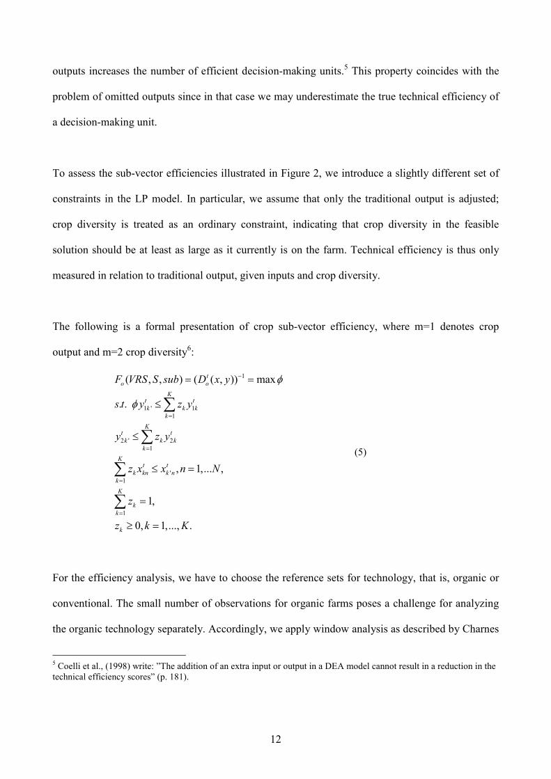
To assess the sub-vector efficiencies illustrated in Figure 2, we introduce a slightly different set of
constraints in the LP model. In particular, we assume that only the traditional output is adjusted;
crop diversity is treated as an ordinary constraint, indicating that crop diversity in the feasible
solution should be at least as large as it currently is on the farm. Technical efficiency is thus only
measured in relation to traditional output, given inputs and crop diversity.
The following is a formal presentation of crop sub-vector efficiency, where m=1 denotes crop
output and m=2 crop diversity6:
1
1 ' 1
1
2 ' 2
1
'
1
1
( , , ) ( ( , )) max
. .
, 1,... ,
1,
0, 1,..., .
t
o o
Kt t
k k k
k
Kt t
k k k
k
Kt t
k kn k n
k
K
k
k
k
F VRS S sub D x y
s t y z y
y z y
z x x n N
z
z k K
φ
φ
−
=
=
=
=
= =
≤
≤
≤ =
=
≥ =
∑
∑
∑
∑
(5)
For the efficiency analysis, we have to choose the reference sets for technology, that is, organic or
conventional. The small number of observations for organic farms poses a challenge for analyzing
the organic technology separately. Accordingly, we apply window analysis as described by Charnes
5 Coelli et al., (1998) write: ”The addition of an extra input or output in a DEA model cannot result in a reduction in the
technical efficiency scores” (p. 181).
13
et al. (1985): observations from several years (in our case four years) are treated as different units.
In traditional window analysis, the earliest period is dropped when a new period is introduced. We
apply a four-year window, or a rotating unbalanced panel. In principle, we take a technical change
into account, as the reference set for the last period in the window includes observations of that year
and the three previous years. However, we cannot totally avoid the problem of a small number of
observations in these comparisons as the averages of technical efficiencies tend to decrease when
the number of observations increases. When the number of observations in the sample increases, the
convergence to the minimum is relatively slow.
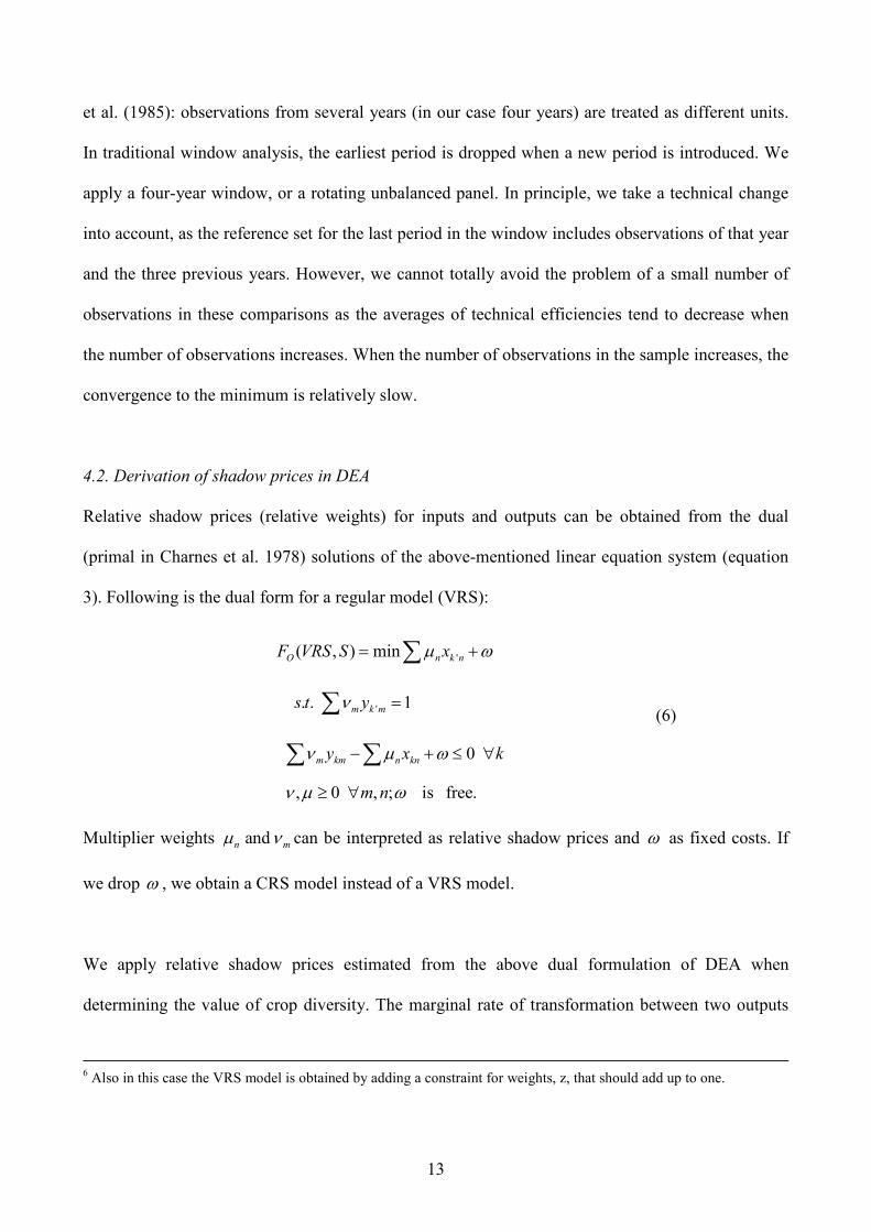
4.2. Derivation of shadow prices in DEA
Relative shadow prices (relative weights) for inputs and outputs can be obtained from the dual
(primal in Charnes et al. 1978) solutions of the above-mentioned linear equation system (equation
3). Following is the dual form for a regular model (VRS):
'
'
( , ) min
. . 1
0
, 0 , ; is free.
O n k n
m k m
m km n kn
F VRS S x
s t y
y x k
m n
µ ω
ν
ν µ ω
ν µ ω
= +
=
− + ≤ ∀
≥ ∀
∑
∑
∑ ∑
(6)
Multiplier weights andn mµ ν can be interpreted as relative shadow prices and ω as fixed costs. If
we drop ω , we obtain a CRS model instead of a VRS model.
We apply relative shadow prices estimated from the above dual formulation of DEA when
determining the value of crop diversity. The marginal rate of transformation between two outputs
6 Also in this case the VRS model is obtained by adding a constraint for weights, z, that should add up to one.
14
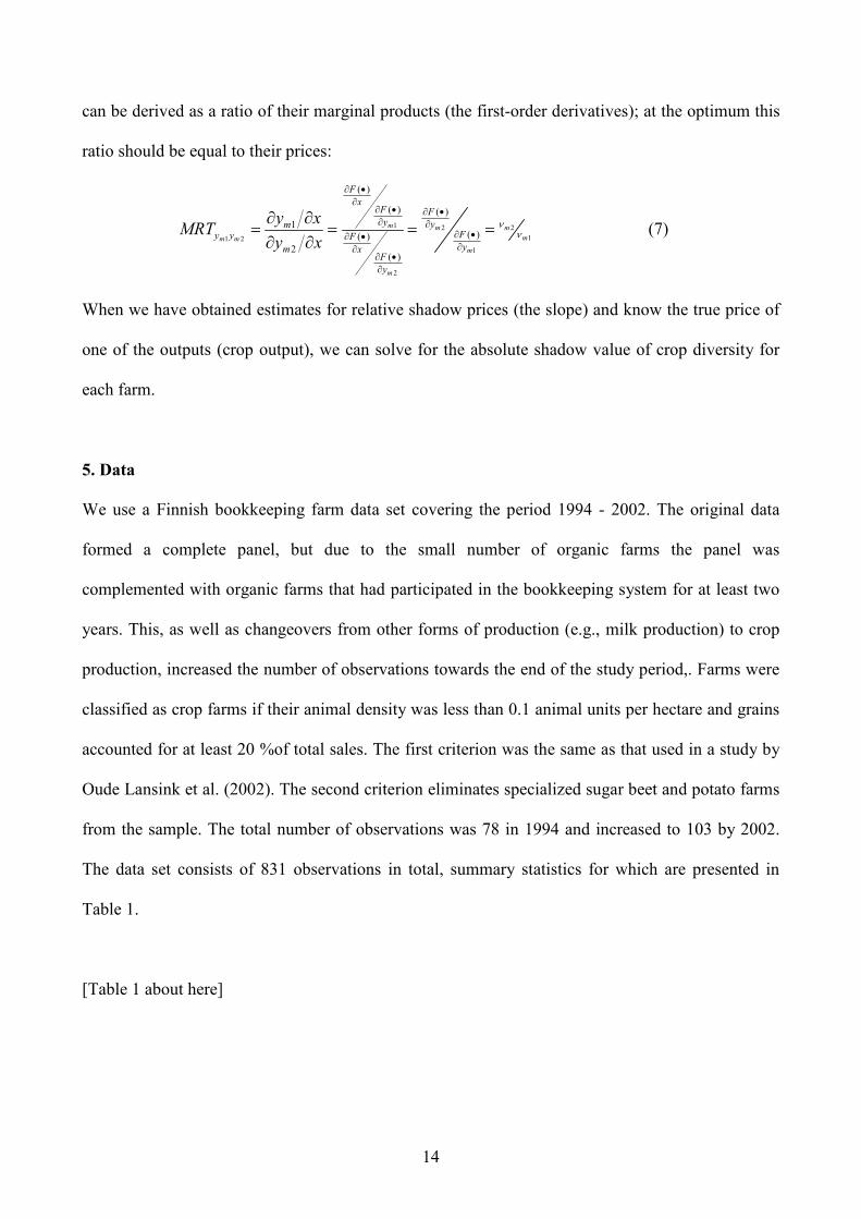
can be derived as a ratio of their marginal products (the first-order derivatives); at the optimum this
ratio should be equal to their prices:
1 2 2
11 2
1
2
( )
( ) ( )
1( )( )
2( )
m m m
mm m
m
m
F
xF Fy ym
Fy y Fym x
F
y
y xMRT
y x
νν
∂ •
∂∂ • ∂ •∂ ∂
∂ •∂ •∂∂
∂ •
∂
∂ ∂= = = =∂ ∂
(7)
When we have obtained estimates for relative shadow prices (the slope) and know the true price of
one of the outputs (crop output), we can solve for the absolute shadow value of crop diversity for
each farm.
5. Data
We use a Finnish bookkeeping farm data set covering the period 1994 - 2002. The original data
formed a complete panel, but due to the small number of organic farms the panel was
complemented with organic farms that had participated in the bookkeeping system for at least two
years. This, as well as changeovers from other forms of production (e.g., milk production) to crop
production, increased the number of observations towards the end of the study period,. Farms were
classified as crop farms if their animal density was less than 0.1 animal units per hectare and grains
accounted for at least 20 %of total sales. The first criterion was the same as that used in a study by
Oude Lansink et al. (2002). The second criterion eliminates specialized sugar beet and potato farms
from the sample. The total number of observations was 78 in 1994 and increased to 103 by 2002.
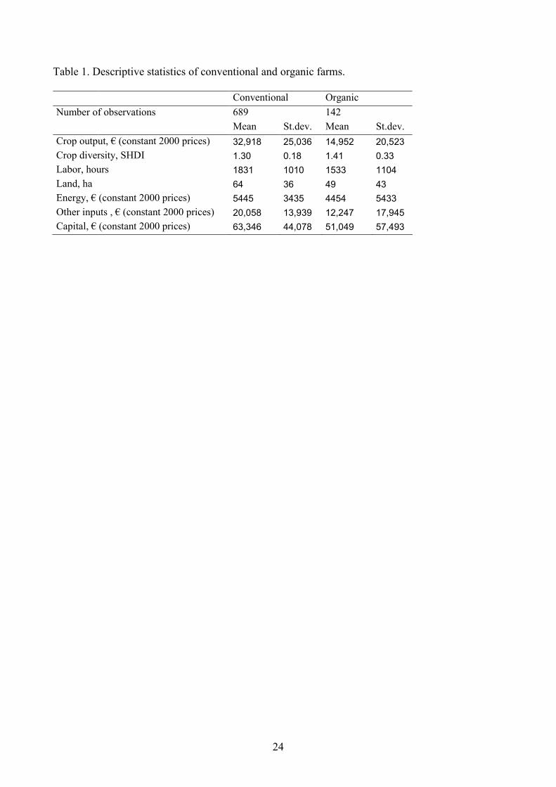
The data set consists of 831 observations in total, summary statistics for which are presented in
Table 1.
[Table 1 about here]
15
The number of organic crop farms was 11 in 1994 and 20 in 2002. We use crop returns as a proxy
of the quantity of aggregate marketable output. Crop output is measured at constant prices for the
year 2000. For both organic and conventional farms, output at constant prices is obtained by
dividing crop returns by the price indices of conventional outputs, published by Statistics Finland7.
The main reason for using price indices for conventionally produced goods only is that we do not
have a reliable index for organic products. In particular, we do not know the exact magnitude of the
price premium for organic production; we have to assume equal prices and price changes for
organic and conventional products, with any price premium for organic products increasing our
proxy of the output quantity. Regardless of any premium, the average traditional crop output is
considerably lower on organic than on conventional farms (see Table 1). All subsidies (direct
payments) paid on the basis of the arable land areas of the farms are excluded.
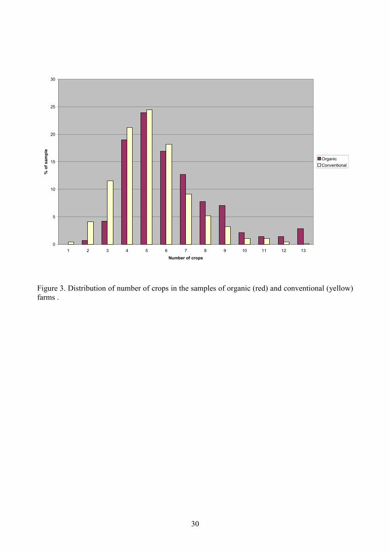
As a measure of a second positive output, or desirable environmental by-product, we use the
Shannon crop diversity index (SHDI), which was discussed in section 2. As Table 1 indicates, the
crop diversity index is on average higher on organic farms.8 Even though the SHDI was chosen as
an indicator because it takes into account the evenness of land use, there is a strong correlation
between THE SHDI and the number of crops cultivated on a farm. The distribution of the number
of crops in the samples of organic and conventional farms is illustrated in Figure 3.
[Figure 3 about here]
7 The division of monetary input or crop output values by respective indices is not necessary if we only analyze the
farms in cross-sections of specific years. However, when we employ a window analysis over time for organic farms, the
use of constant monetary values is necessary.
8 The t-test statistics for differences in output and crop diversity index were 9.13 and 3.86, respectively.
16
The outputs are produced by using five inputs. Labor is measured in hours as a sum of family and
hired labor input. Land is measured in hectares corresponding to the total arable land area of the
farm. The input variables accounted for at constant 2000 prices are energy, comprising both fuel
and electricity, other supplies such as purchased fertilizers, seed, and feed, and capital, including the
value of buildings and machinery. The respective input price indices are obtained from Statistics
Finland. The average arable land area of conventional farms is about 15 hectares larger than that of
organic farms, a difference that is statistically significant (t-test statistics 4.09). Conventional farms
consume on average more of all inputs than organic farms.
When comparing crop farms we observed very low crop output values in some cases. Low output
relative to inputs yields a low technical efficiency score. However, it is difficult to determine
whether these observations should be regarded as outliers and on which grounds. Therefore, no
observation has been dropped.
6. Results
6.1 Efficiency scores for conventional and organic farms
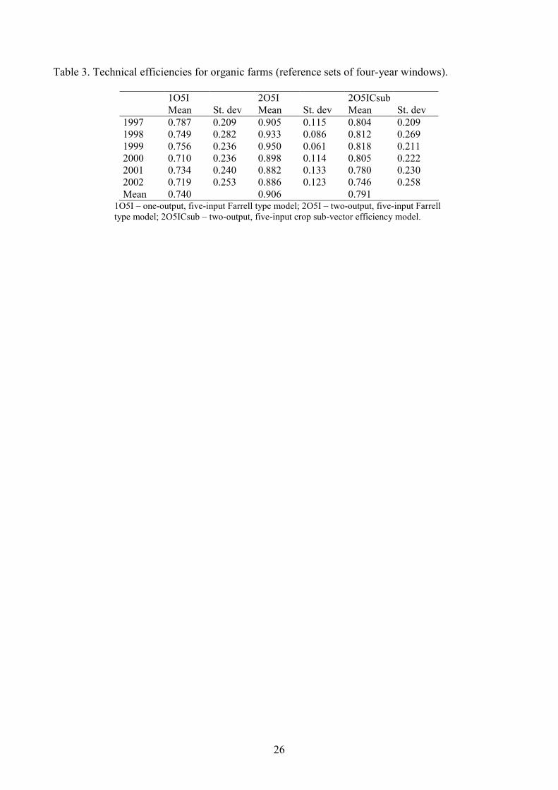
We apply DEA to separate data sets of conventional and organic farms. For organic farms, we use
window analysis assuming progressive technical change. This assumption means that, for example,
the efficiency scores for 1997 are calculated using the observations from 1994 to 1997 as the
reference set but the mean is calculated on the basis technical efficiencies of the farms observed in
19979. Using several years’ observations as the reference set for organic farms increases the number
of dimensions in the DEA to almost that in the annual analysis of conventional farms (without a
window).
9 When we apply a four-year window and assume technical progress we cannot calculate mean efficiencies in the period
1994- 1996.
17
The results for separate data sets for conventional and organic farms (window analysis for the latter)
are presented in Tables 2 and 3. First, we estimate the Farrell type technical output efficiencies
applying a model of one output (crop output) and five inputs and variable returns to scale (equation
4). The results are presented in the column headed 1O5I. Second, we take into account the
biodiversity effects of production by including crop diversity as an output in addition to the
traditional crop. The traditional output is sold on the market; crop diversity is a non-marketable
effect. For the two-output case, efficiency scores are reported in column 2O5I. Finally, a sub-vector
efficiency model for two outputs and five inputs is applied; crop sub-vector efficiency is found in
column 2O5ICsub.
The means of the technical efficiency scores for the two farming technologies seem to be very
close, but the pattern of change varies: for the conventional farms the average technical efficiencies
are at their lowest level in 1998 and 1999, and at their highest in 2000; for the organic farms,
efficiency peaks in 1999 in the two-output models, and decreases constantly thereafter in the crop
sub-vector efficiency model. This variation may be explained by the differences in how the
reference sets were constructed.
[Tables 2 and 3 about here]
We should point out that the number of observations on which the annual average technical
efficiencies of organic farms are based is only 14-2010. However, the results suggest that the
average efficiencies in the two technologies do not differ markedly as can be seen from Tables 2
and 3. The result is independent of the model on which the analysis is based. Here, it should be
10 The number of annual observations in the last year of the window.
18
pointed out that the results were rather similar in the two-output model even when we used number
of crops instead of the SHDI as an indicator of ecological diversity.
6.2 Shadow values, or opportunity costs, of crop diversity
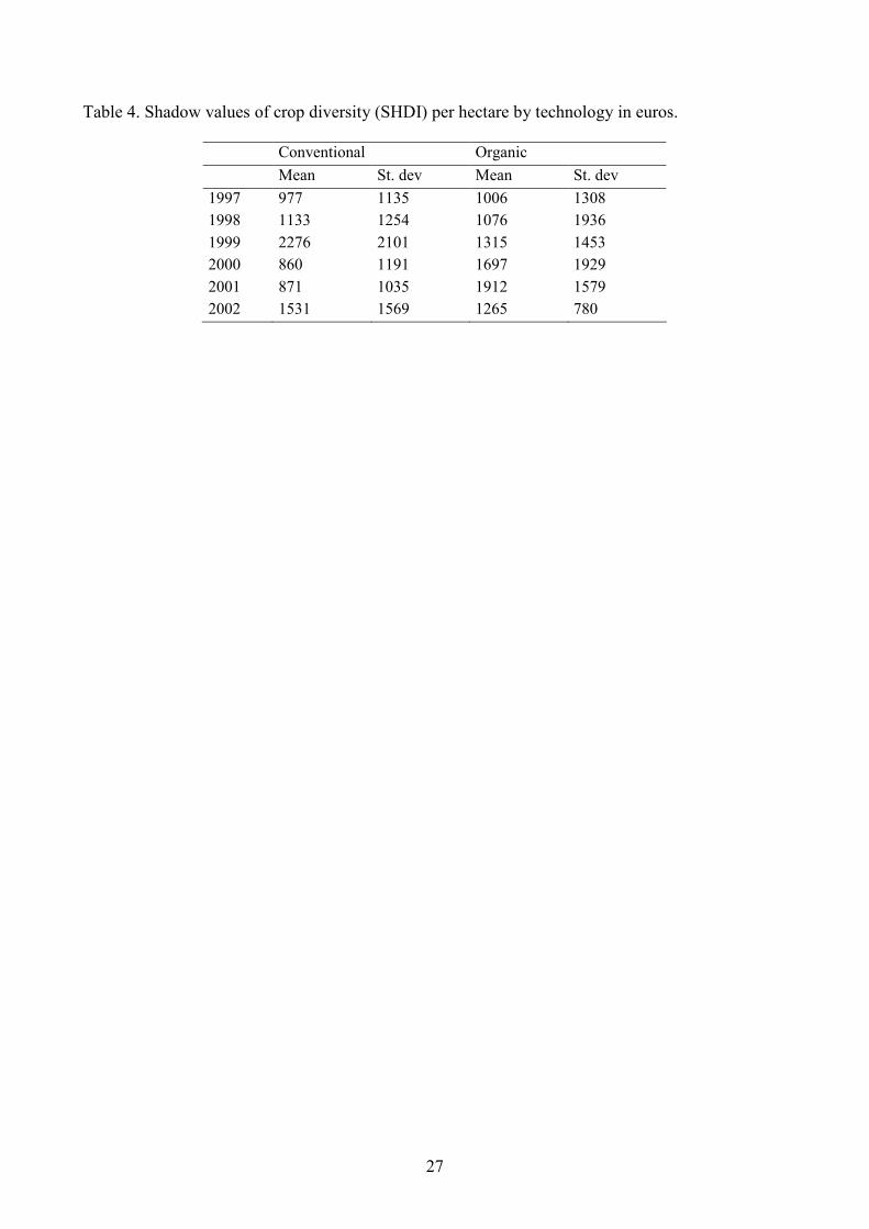
We apply the dual formulation of DEA to calculate shadow values for crop diversity using
equations (6) and (7). When calculating the shadow value for crop diversity, we assume that the
actual price of one unit of crop output is EUR 1 at the 2000 price.
Table 4 presents the shadow values based on the separate efficiency estimations of organic and
conventional technologies. We only compare the results of non-zero shadow values from 1997 to
2002, since we apply window analysis to the group of organic farms. In addition, the distribution of
shadow values of crop diversity is truncated at EUR 10,000 in order to exclude some extreme
values (four observations for organic and ten for conventional farms).
[Table 4 about here]
The differences in shadow values between technologies are statistically significant for the years
1999, 2000 and 2001. However, variation in the shadow values is large in both samples, and the
mean values do not follow any specific pattern over the time period considered.
The shadow values provide important information for policy design,. The values reflect the
opportunity costs to farms of increasing crop diversity. Therefore, the observations indicating the
least cost have been ordered by the estimated shadow values, or opportunity costs (per hectare), of
19
increasing crop diversity (SHDI) by one unit. It should be noted that an increase of one unit in the
SHDI is quite considerable, although this is a matter of the scale chosen.
[Figure 4 about here]
Figure 4 illustrates the shadow values for 40 % of total land area in both samples; the highest values
reach EUR 1000 per hectare for the organic and almost EUR 600 per hectare for the conventional
sample. The lowest opportunity costs in the figure can be interpreted as supply curves for crop
diversity. The curves cross at about EUR 300 per hectare of a unit of THE SHDI. The opportunity
costs of organic farms are systematically smaller for a land area of less than 20 %, that is, up to the
crossing point. For these least-cost farms, the opportunity cost of crop diversity is on average EUR
165 per hectare for conventional farms and EUR 130 per hectare for organic farms, a difference of
roughly 25 %. The least-cost farms are the most promising candidates for receiving conservation
payments if auctions are expected to increase cost efficiency in the conservation of crop diversity
on farmland. On the remaining 80 % of the farmland, the opportunity costs of crop diversity are
higher and increase more rapidly on organic than on conventional farms.
7. Conclusions
Consideration of the concrete environmental benefits to be achieved is important for the design of
agri-environmental policies. The present study integrates such benefits into the production process
as a desirable output and compares conventional and organic technologies using the Shannon crop
diversity index. The index takes into account both richness and evenness, but one could
alternatively focus on richness only and use number of crops as an ecological indicator.
20
In our sample, organic farms had on average slightly higher crop diversity than conventional farms.
The technical efficiency scores for the two farming technologies seem to be relative close to each
other, and the inclusion of crop diversity as a positive output does not change the relative
performance of the two farm types in any systematic manner. Yet, the opportunity costs of crop
diversity are on average higher for conventional than organic farms up to 20 % of their least-cost
farming area. Above that share, that is, on the remaining 80 % of the farm land, the opportunity
costs of crop diversity increase more rapidly for organic than for conventional farms.
Although crop diversity as a policy goal cannot be justified by an expected increase in the value of
crop output in the short run, crop diversity may provide economic benefits in the long run and other
benefits that are not related to agricultural productivity. Even though our approach is only a first
step towards analyzing the economic and environmental impacts of alternative farming technologies
simultaneously, the thrust of our analysis is clear. Normally, there is a trade-off between several
outputs. Multiple outputs, including environmental impacts, should be accounted for, given that the
efficiency ranking of alternative technologies is dependent on what is actually considered as
outputs. It is important to identify the heterogeneity of farms in producing environmental benefits if
tailored agri-environmental policies are to lead to cost efficiency and savings in the use of
taxpayers’ money.
Further research is needed on elaborating other environmental benefit indices that can be calculated
on the basis of the farm accountancy data available to regulators. In our analysis, we have
concentrated on the annual variation in diversity at the farm level. If landscape values are evaluated,
the scale of analysis should be extended beyond the borders of farm units. Studies incorporating
aggregation over farms and time would enable more informed policy assessments.
21
References
Armsworth, P.R., Kendall, B.E. and Davis, F.W. (2004). An introduction to biodiversity concepts for
environmental economists. Resource and Energy Economics 26: 115–136.
Bastian, C., Menkhaus, D., Nagler, A. and Ballenger, N. (2008). “Ex Ante” Evaluation of Alternative
Agricultural Policies in Laboratory Posted Bid Markets. American Journal of Agricultural Economics 90(5):
1208–1215.
Benton, T.G., Vickery, J.A. and Wilson, J.D. (2003). Farmland biodiversity: is habitat heterogeneity the key?
TRENDS in Ecology and Evolution 18(4): 182–188.
Callicott, J.B., Crowder, L.B. and Mumford, M.R. (1999). Current normative concepts in conservation.
Conservation Biology 13: 22–35.
Chambers, R.G., Chung, Y. and Färe, R. (1998). Profit, directional distance function, and Nerlovian
efficiency. Journal of Optimization Theory and Applications 98(2): 351–364.
Charnes, A., Cooper, W.W. and Rhodes, E. (1978). Measuring the inefficiency of decision making units.
European Journal of Operational Research 2: 429–444.
Charnes, A., Clark, T., Cooper, W.W. and Golany, B. (1985). A developmental study of data envelopment
analysis in measuring efficiency of maintenance units in U.S. Air Forces. Annals of Operational Research 2:
95–112.
Coelli, T., Rao, D.S.P. and Battese, G.E. (1998). An introduction to efficiency and productivity analysis.
Kluwer Academic Publishers.
Debreu, G. (1951). The coefficient of resource utilization. Econometrica 19(3): 273–292.
Di Falco, S. and Perrings, C. (2005). Crop biodiversity, risk management and the implications of agricultural
assistance. Ecological Economics 55: 459–466.
Farrell, M.J. (1957). The measurement of productive efficiency. Journal of the Royal Statistical Society.
Series A, 120: 253–281.
Feng, H. (2007). Green payments and dual policy goals. Journal of Environmental Economics and
Management 54: 323–335.
Färe, R. and Grosskopf, S. (1998). Shadow Pricing of Good and Bad Commodities. American Journal of
Agricultural Economics 80: 584–590.
Färe, R., Grosskopf, S. and Lovell, C.A.K. (1994). Production frontiers. Cambridge.
Färe, R., Grosskopf, S. and Weber, W.L. (2001). Shadow prices of Missouri public conservation land. Public
Finance Review 29(6): 444–460.
Glebe, T. (2008). Scoring two-dimensional bids: how cost-effective are agri-environmental auction.
European Review of Agricultural Economics 35(2): 143–165.
Groth, M. (2009). The transferability and performance of a payment-by-result approach and conservation
procurement auctions for cost-effective biodiversity conservation: results of a case-study in Northern
22
Germany. Paper presented at the 17th Annual Conference of the European Associations of Environmental and
Resource Economists.
Herzog, F., Steiner, B., Bailey, D., Baundry, J., Billeter, R., Bukácek, R., De Blust, G., De Cock, R.,
Dirksen, J., Dormann, C.F., De Filippi, R., Frossard, E., Liira, J., Schmidt, T., Stöckli, C., Thenail, C., van
Wingerden, W. and Bugter, R. (2006). Assessing the intensity of temperate European agriculture at the
landscape scale. European Journal of Agronomy 24: 165–181.
Hietala-Koivu, R., Lankoski, J. and Tarmi, S. (2004). Loss of biodiversity and its social cost in an
agricultural landscape. Agriculture, Ecosystem and Environment 103: 75–83.
Horisontaalinen maaseudun kehittämisohjelma 2006. Manner-Suomea koskevat EU:n yhteisen
maatalouspolitiikan liitännäistoimenpiteet vuosille 2000 – 2006 (In Finnish). Ministry of Agriculture and
Forestry.
http://www.mmm.fi/attachments/maaseutu/maaseudunkehittamisohjelmat/horisontaalinenmaaseudunkehitta
misohjelma/5lK0r8BYB/horisontaaliohjelma.pdf (referred January 8, 2010)
Huhtala, A. and Marklund, P.-O. (2008). Stringency of environmental targets in animal agriculture: shedding
light on policy with shadow prices. European Review of Agricultural Economics 35(2): 193–217.
Jackson, L.E., Pascual, U. and Hodgkin, T. (2007). Utilizing and conserving agrobiodiversity in agricultural
landscapes. Agriculture, Ecosystems and Environment 121: 196–210.
Karlen, D.L., Varvel, G.E., Bullock, D.G. and Cruse, R.M. (1994). Crop rotations for the 21st century.
Advanced Agronomy 53: 1–44.
Keylock, C.J. (2005). Simpson diversity and the Shannon-Wiener index as special cases of a generalized
entropy. Oikos 109(1): 203–207.
Kirwan, B., Lubowski, R.N. and Roberts, R.N. (2005). How cost-effective are land retirement auctions?
Estimating the difference between payments and willingness to accept in the conservation reserve program.
American Journal of Agricultural Economics 87: 1239–1247.
Koopmans, T.C. (1951). An analysis of production as an efficient combination of activities. In: T.C.
Koopmans (ed.), Activity analysis of production and allocation. Cowles Commission for Research in
Economics. Monograph 13. New York: John Wiley and sons, Inc.
Latacz-Lohman, U. (2004). Dealing with limited information in designing and evaluating agri-environmental
policy. Paper presented in 90th EAAE seminar on 28.–29.10.2004, Rennes, France. 17 p.
Latacz-Lohman, U. and Schilizzi, S. (2005). Auctions for conservation contracts: A review of the theoretical
and empirical literature. Report to the Scottish Executive Environment and Rural Affairs Department.
Latacz-Lohman, U. and van der Hamsvoort, C. (1997). Auctioning Conservation Contracts: A Theoretical
Analysis and an Application. American Journal of Agricultural Economics 79(2): 407–418.
McGarical, K. and Marks, B.J. (1995). FRAGSTATS: Spatial pattern analysis program for quantifying
landscape structure. USDA Forest Services. PNW-GTR-351. Portland, OR, USA.
Miettinen, A., Lehtonen, H. and Hietala-Koivu, R. (2004). On diversity effects of alternative agricultural
policy reforms in Finland: An agricultural sector modelling approach. Agricultural and Food Science 13(3):
229–246.
23
Organic Farming in the EU: Facts and Figures (2005).
http://ec.europa.eu/agriculture/organic/files/eu-policy/data-statistics/facts_en.pdf (referred January 8, 2010)
Oude Lansink, A., Pietola, K. and Bäckman, S. (2002). Efficiency and productivity of conventional and
organic farms in Finland 1994-1997. European Review of Agricultural Economics 29(1): 51–65.
Pacini, C., Wossink, A., Giesen, G., Vazzana, C. and Huirne, R. (2003). Evaluation of sustainability of
organic, integrated and conventional farming systems: A farm and field-scale analysis. Agriculture,
Ecosystems and Environment 95: 273–288.
Pascual, U. and Perrings, C. (2007). Developing incentives and economic mechanisms for in situ biodiversity
conservation in agricultural landscapes. Agriculture, Ecosystems and Environment 121: 256–268.
Piot-Lepetit, I. and Vermersch, D. (1998). Pricing organic nitrogen under the weak disposability assumption:
An application to the French pig sector. Journal of Agricultural Economics 49: 85–99.
Piot-Lepetit, I. and Le Moing, M. (2007). Productivity and environmental regulation: the effect of the
nitrates directive in the French pig sector. Environmental and Resource Economics 38(4): 433–446.
Riedell, W.E., Schumacher, T.E., Clay, S.A., Ellsbury, M.M., Pravecek,M. and Evenson, P.D. (1998). Corn
and soil fertility responses to crop rotation with low, medium, or high inputs. Crop Science 38: 427–433.
Shannon, C.E. (1948). A mathematical theory of communication. Bell System Technical Journal 27: 379–
423, 623–656.
Shephard, R.W. (1953). Cost and production functions. Princeton: Princeton University Press.
Shephard, R.W. (1970). Theory of cost and production functions. Princeton: Princeton University Press.
Sheriff, G. (2009). Implementing second-best environmental policy under adverse selection. Journal of
Environmental Economics and Management 57: 253–268.
Struik, P.C. and Bonciarelli, F. (1997). Resource use of cropping system level. European Journal of
Agronomy 7: 133–143.
Watson, C.A., Atkinson, D., Gosling, P. Jackson, L.R. and Rayns, F.W. (2002). Managing soil fertility in
organic farming systems. Soil Use Management 18: 239–247.
van Wenum, J.H., Wossink, G.A.A. and Renkema, J.A. (2004). Location specific modeling for optimizing
wildlife management on crop farms. Ecological Economist 48: 395–407.
Wossink, G.A.A. and van Wenum, J.H. (2003). Biodiversity conservation by farmers: analysis of actual and
contingent valuation. European Review of Agricultural Economics 30(4): 461–485.
24
Table 1. Descriptive statistics of conventional and organic farms.
Conventional Organic
Number of observations 689 142
Mean St.dev. Mean St.dev.
Crop output, € (constant 2000 prices) 32,918 25,036 14,952 20,523
Crop diversity, SHDI 1.30 0.18 1.41 0.33
Labor, hours 1831 1010 1533 1104
Land, ha 64 36 49 43
Energy, € (constant 2000 prices) 5445 3435 4454 5433
Other inputs , € (constant 2000 prices) 20,058 13,939 12,247 17,945
Capital, € (constant 2000 prices) 63,346 44,078 51,049 57,493
25
Table 2. Technical efficiencies for conventional farms (annual reference sets).
1O5I 2O5I 2O5ICsub
Mean St. dev Mean St. dev Mean St. dev
1997 0.771 0.177 0.911 0.095 0.832 0.177
1998 0.671 0.203 0.834 0.132 0.717 0.215
1999 0.663 0.241 0.872 0.129 0.735 0.246
2000 0.835 0.154 0.903 0.113 0.867 0.150
2001 0.728 0.189 0.878 0.115 0.789 0.190
2002 0.723 0.196 0.897 0.099 0.793 0.183
Mean 0.734 0.883 0.791 1O5I – one-output, five-input Farrell type model; 2O5I – two-output, five-input Farrell
type model; 2O5ICsub – two-output, five-input crop sub-vector efficiency model.
26
Table 3. Technical efficiencies for organic farms (reference sets of four-year windows).
1O5I 2O5I 2O5ICsub
Mean St. dev Mean St. dev Mean St. dev
1997 0.787 0.209 0.905 0.115 0.804 0.209
1998 0.749 0.282 0.933 0.086 0.812 0.269
1999 0.756 0.236 0.950 0.061 0.818 0.211
2000 0.710 0.236 0.898 0.114 0.805 0.222
2001 0.734 0.240 0.882 0.133 0.780 0.230
2002 0.719 0.253 0.886 0.123 0.746 0.258
Mean 0.740 0.906 0.791 1O5I – one-output, five-input Farrell type model; 2O5I – two-output, five-input Farrell
type model; 2O5ICsub – two-output, five-input crop sub-vector efficiency model.
27
Table 4. Shadow values of crop diversity (SHDI) per hectare by technology in euros.
Conventional Organic
Mean St. dev Mean St. dev
1997 977 1135 1006 1308
1998 1133 1254 1076 1936
1999 2276 2101 1315 1453
2000 860 1191 1697 1929
2001 871 1035 1912 1579
2002 1531 1569 1265 780
28
Figure 1. Technical output efficiency in the case of crop output and crop diversity.
Technology 1
0
Crop output
g f
e
Technology 2
Crop diversity
29
Figure 2. Traditional and sub-vector technical efficiencies.
Crop sub-vector
efficiency
0
Crop output
A
Crop diversity
Crop diversity sub-vector
efficiency
Radial technical
efficiency
30
0
5
10
15
20
25
30
1 2 3 4 5 6 7 8 9 10 11 12 13
Number of crops
% of sample
Organic
Conventional
Figure 3. Distribution of number of crops in the samples of organic (red) and conventional (yellow)
farms .

31
0
200
400
600
800
1000
1200
0 1 2 3 4 5 7 8 8
10
11
12
12
14
15
15
16
17
18
19
20
21
23
24
24
25
26
28
29
30
31
32
34
35
36
37
39
39
of sample area (%)
euro/ha
Organic Conventional
Figure 4. Shadow values of crop diversity for organic and conventional farms.