Embed Size (px)
Citation preview
1
Do voters really tolerate corruption?
Evidence from Spanish Mayors
Elena Costas, Albert Solé-Ollé & Pilar Sorribas-Navarro
Universitat de Barcelona & Institut d’Economia de Barcelona (IEB)
ABSTRACT:
We analyze the effects of local corruption on electoral outcomes with Spanish data. Based upon press reports published between 1996 and 2009, we are able to construct a novel database on corruption scandals and corruption news related to bribe-taking in exchange of amendments in land use plans. With this data, we estimate an incumbent’s vote share equation for the 2007 and 2003 municipal elections. Most previous studies on this topic fail to account for the omission of popularity shocks. By using both ‘difference-in-differences’ (DD) and ‘instrumental variables’ (IV) methods, we show that while often the punishment is modest, when the appropriate circumstances concur, corrupt politicians are punished with a higher intensity than usually believed. DD results suggest that the average vote loss after a corruption scandal is quite low (around 3%), but that this effect is bigger for cases widely reported by newspapers (up to 9%), and also for cases with direct intervention of the judiciary (up to 12%). IV effects are somewhat higher (up to 17%).
Keywords: voting, accountability, corruption JEL Classification: P16, D72
* Corresponding author: Albert Solé-Ollé ([email protected]).This research has received funding from projects ECO2009-12680/ECON (Ministerio de Educación y Ciencia) and 2009SGR102 (Generalitat de Catalunya).

2
1. Introduction
Corruption is a complex phenomenon, and its negative political and economic cones-
quences have been widely analyzed in recent years. Corruption is said to erode trust in
government and the legitimacy of political institutions (Anderson and Tverdova 2003;
Bowler and Karp, 2004) and also to deter investment (e.g. Wei, 2000) and reduce
growth (e.g. Mauro, 1995). Institutions as the World Bank point out at corruption as the
single most important impediment to development. Being the impact of corruption so
potentially devastating, knowing about the institutions that would help to mitigate it
seems of crucial importance. One of the main results of the recent literature on the
institutional determinants of corruption (e.g. Treisman, 2000; Lederman et al., 2005) is
that advanced democracies are less corrupt than other political systems. Key ingredients
of democracy, as party-based competition, free elections, press freedom, or an indepen-
dent judiciary, are correlated with lower levels of political corruption (e.g. Goldsmith,
1999; Besley and Burgess, 2002; Adserà et al., 2003; Alt and Lassen, 2008; van Aaken
et al., 2010).
The basic mechanism that makes democracy work is the capacity that voters have to
held politicians accountable, ousting them form office if there are evidences of corrup-
tion, and rewarding honest behavior with re-election. Yet, most of the empirical studies
that have addressed this question tended to find just modest effects of corruption on
candidate’s votes. For example, regarding a case-study of corruption in Japan, Reed
(1999) notes that the percent of votes lost by legislators indicted of corruption during
the period 1947-93 was around 11%. Similar results were found by the study of Peters
and Welch (1980) on the electoral impact of corruption charges on the vote for candida-
tes to the U.S. House of representatives during the period 1968-78. They estimate that
candidates accused of corruption lost between 6% and 11% of the vote, depending on
her being a Republican or a Democrat. An update of this study for the period 1982-90
(Welch and Hibbing, 1997) found somewhat higher results, with an average loss of vote
of 10%, and lower probabilities of re-election for corrupt politicians. In their analysis of
the House check kiting scandal in 1992, Dimock and Jacobson (1995) find that most
incumbents managed to be reelected, albeit with a reduced vote share of around 5%.
This number does not account, however, for the fact that most offenders choose to retire
rather than accept the risk of an electoral defeat (Banducci and Karp, 1994).

3
Note that all these studies focus on the behavior of legislators. There are nearly no
studies analyzing the effect of corruption on the electoral prospects of other officials
and, specially, of mayors, which are the focus of this paper1. One prominent exception
is the article by Ferraz and Finan (2008) on Brazilian mayors2. They find big electoral
punishment against mayors when voters are provided with conclusive evidence of
corruption, in form of federal audits of municipal records showing diversion of funds.
Mayors found corrupt by an audit before the election date might loss from 10% to 30%
of the vote share and see the re-election probability reduced by a 17%. The reduction in
re-election probabilities are even bigger (up to 30%) in municipalities with a radio
station. The authors claim that the bigger effects, as compared with the other studies, are
due to the fact that they use data on corruption evidence and not just on corruption
scandals. However, Golden (2006) suggests that the result might be also due to the
direct relationship between ousting a corrupt mayor and improving public services,
which is less certain in the case of a legislator than is for a mayor. Another explanation
for the results is the quasi-experimental nature of the audit data that helps to overcome
the omitted popularity bias which plagues this type of studies and which tends to bias
negatively the estimated effect of corruption on the vote.
The present study aims at enlarging this body of empirical evidence by analyzing the
effects of corruption on local electoral outcomes with Spanish data, focusing on the
2007 and 2003 municipal elections. Based upon press reports published between 1996
and 2009 we are able to construct a novel database on corruption scandals and corrupt-
tion news related to bribe-taking in exchange of amendments in land use plans, allowing
for more development to take place. The source of this data comes from ‘Fundación
Alternativas’, a Spanish think tank, which in 2007 commissioned a survey that scanned
all corruption scandals as reported by national, regional and local newspapers during the
period 2000-2007. This database was complemented by a Bibliographical news search
for the years before and after this period. Overall, we have in our database 666 munici-
palities with at least one corruption scandal during the period 1999-2007 (which covers
the two terms we finally analyze) and 5329 news about corruption. For the 2003-2007
1 Note that this is despite the existence of some recent papers that argue that accountability can be strengthened at the local level (see, e.g. Bardhan, 1997, and Seabright, 1998). 2 Another paper on Brazilian mayors by Brollo (2008) corroborates these results but show that corrupt municipalities are punished not only by voters but also by the central government, with a reduction of intergovernmental transfers.
4
term, we also have information on the type of scandal, being just media reporting of a
public accusation made by a party or any other organization, or real charges of
corruption involving intervention of the judiciary. The richness of the database allows
not only to evaluate the average impact of corruption scandals on the incumbent’s vote,
but also to assess the role of media reporting (i.e. number of news, type of newspaper)
and the effect of judiciary intervention (i.e. investigation, accusation, conviction).
There are several reasons that make the Spanish case interesting. First, local corruption
was not an issue before the elections we analyze. The sudden appearance of corruption
in the Spanish local political life is the result of the recent big construction boom, which
can be considered an exogenous factor. Second, Spanish local corruption refers to
corruption related to land use regulations, a type of corruption rarely studied in the
literature (see Cai et al., 2009, for an exception). The highly interventionist and discre-
tionary nature of Spanish land use regulations are the channel that transformed the
demand shock into corruption scandals. In Spain, municipalities are responsible for
passing very detailed land use plans, which fix the exact amount of land allowed to be
developed during a given period, and the conditions of this development. Shortage of
vacant land (and, more generally, restrictive regulations), coupled with a huge demand
shock, provides developers with incentives to offer bribes to local officials in exchange
of amendments in the plan to allow for more construction, either on the extensive
margin (more land being built-up, see Solé-Ollé and Viladecans, 2010) or on the inten-
sive one (increasing construction density).
There are some specifics related to this type of corruption that potentially affect the
results obtained. It is a very homogeneous type of corruption, something very difficult
to find in empirical cases of corruption that mix very different types of violations, some
of them related with the concept of corruption (e.g. bribes, procurement fraud, resource
diversion) but other farther away from it (as, e.g. financial irregularities, poor manage-
ment, or other types of crime3). Moreover, the nature of the corrupt act, which entails
changing a regulation and does not affect directly the budget of the municipality, means
it might be perceived differently by voters than the more traditional theft-related
violations (e.g. those studied in Ferraz and Finan, 2008). Laxer land use regulations do
3 This type of problem affects the U.S. data on convictions by state (see Glaeser and Saks, 2006) or the database on corruption by Italian legislators (see Golden et al., 2010).

5
have some effects that might be valued positively by some voters, blurring the negative
perception of corruption. For instance, politicians accepting bribes in exchange of
permitting more development might be seen by some voters as entrepreneurs taking part
of the profit they secure for the community in terms of higher economic opportunities
related to new development.
Third, Spanish local corruption scandals had a wide coverage by the media during these
years, with news appearing in the main newspapers every day for extended periods.
Despite this, there is anecdotal evidence that some corrupt mayors (even some of the
convicted ones), were re-elected and even improved their vote shares. Newspaper
opinions on these cases reflect the popular wisdom that ‘Spanish voters do tolerate
corruption’4. Majoritarian elections with closed lists, lack of independent media, low
transparency of local policy-making (see Transparency International, 2007), clientelism
and patronage networks5, and a culture of tolerance to fraud (Fundación Alternativas,
20086) have been often invoked to justify these results. Thus, Spain seems a very good
testing ground to check the validity of some of these claims in a more formal way.
We use the corruption data to estimate an incumbent’s vote share equation for the 2007
and 2003 municipal elections. Most previous studies on this topic fail to account for the
omission of popularity shocks. We use both ‘difference-in-differences’ (DD) and ‘ins-
trumental variables’ (IV) methods to attenuate this problem. Our DD estimation compa-
res the increase in the vote for the incumbent in two consecutive elections relative to the
increase experienced by the previous incumbent in municipalities with and without a
corruption scandal during the term. Our IV estimation exploits the dynamics of the
construction boom during the period analyzed, using as instruments interactions
between demand shock proxies (e.g. being a beach town multiplied by the average extra
growth in beach towns during each term-of-office) and the amount of vacant land at the
4 For example, a special report on corruption cases in Andalucía (a southern Spanish region) by El País (one the main national newspapers) in 2007 was headlined as ‘The polls forgive charged officials’ (‘ Las urnas perdonan a los imputados’, El País, 5/29/2007. The journal documented that 30 of the 40 officials with corruption charges before the 2003 local elections were reelected. 5 A recent article in El País put it this way: “Corrupt politicians are those that don’t reach office alone but that able to colonize the administration with the members of a clientelism network, and this is quite easy in Spain” (‘La paradoja de la corrupción’, El País, 05/04/2010). 6 For instance, this report claims that generalized tax evasion in Spanish real state taxation (e.g. registration of housing purchase prices lower than real in order to reduce payments of the land transaction tax, hiding rent payments which are subject to tax under the Spanish income tax) could be responsible to the voters’ lax evaluation of housing-related corruption by local officials.
6
beginning of the period, which proxies the difficulties developers face in trying to built
without having to resort to paying bribes.
Our results show that, while vote losses are on average modest, when the appropriate
circumstances concur, corrupt politicians are punished by the voters with a higher
intensity than usually believed. DD results suggest that the mean vote loss after a
corruption scandal is quite low (around 3%), but that this effect is bigger for cases
widely reported by newspapers (up to 9%), and also for cases with direct intervention of
the judiciary (up to 12%). IV effects are higher, up to 17%. The effects are also quite
heterogeneous, left-wing governments being more punished than right-wing ones, and
punishment being also lower in municipalities with high unemployment, high share of
construction employment, and low job mobility (low percentage of commuters).
The paper is organized as follows. In the next section we provide basic background on
the Spanish case of study, including details about the construction of the database, and
describing the recent corruption surge and the role that land use planning has played in
it. Section three discusses our empirical strategy and presents the results and section
four concludes.
2. Corruption in Spanish local governments
2.1 Measuring local corruption: the database
Empirical studies of corruption use at least three different approaches to get the required
data. First, most of them use to work with corruption perceptions (e.g. Wei, 2000;
Alesina and Weder, 2002). The problem with perceptions of corruption is that they
might be biased (see Olken, 2009), their dynamic evolution can be different that the one
of corruption occurrences (see Ujhelyi and Donchev, 2010), and they are not generally
available at the sub-national level of analysis (unless a specific survey is commissioned,
as in Olken, 2009). Second, there are some papers that had access to public records on
corruption charges (see, e.g. Glaeser and Saks, 2006; Alt and Lassen, 2008; Leeson and
Sobel, 2008), the problem in this case being that they mix in the same measure very
different kinds of violations, sometimes no related to corruption. Just a few works have
sufficiently rich data to ensure that the measure of corruption they use is not
contaminated in this way (Ferraz and Finan, 2008; Golden et al., 2010). Third, being
difficult to access to this kind of data at the local level, recently some authors turned to

7
use Bibliographical and/or Internet-guided searches (Glaeser and Goldin, 2004; Sáez
and Simonsohn, 2007). The problem in this case is the difficulty of separating real cases
of corruption, where politicians have really been charged by the judiciary from cases
that have been reported by the press after public denounces of political parties and other
organizations. The main advantage of this approach is that it accounts for corruption
only if voters had access to information about it. In analysis focusing on agents’
reactions to corruption this is more relevant than the real occurrence of corruption
(which nevertheless could go unnoticed by voters if the media did find interesting its
coverage). Another advantage rests upon the fact that the count of the number of news
or citations provides a natural way to measure not just the occurrence of a corruption
case but its severity.
Our approach combines the third and second methods. We had access to a database on
corruptions scandals compiled by Fundación Alternativas (2007), a Spanish think-tank.
In 2007, just after the big surge of corruption scandals that occurred in 2006, this orga-
nization commissioned a survey of local corruption in order to gauge quantitatively the
real relevance of the phenomenon. They hired a journalist in each of the fifty Spanish
provinces with the task of compiling all the corruption news related to municipalities in
the province that appeared from 1-January-2000 to 1-February-2007 in national, region-
nal or local newspapers, and that were related to this period or to the past. The search
found a total of 701 corruption cases occurred since 1991 (see Table 1).
[Insert Table 1]
Before deciding to use this database we made some checks regarding its reliability.
Fundación Alternativas is an organization with close links to the socialist party (PSOE),
and we were concerned about the possible partisan bias of the database. Our suspicions
arise because we know, for example, that the main left-wing Spanish newspaper (‘El
País’) started in 2006 a crusade against corruption, with daily news on corruption
scandals affecting the main right-wing party (Partido Popular, PP). To check for this
possibility we compared this database with another one compiled with the right-wing
newspaper ‘El Mundo’7. This comparison reveals that the proportion of corruption
7 This database covers the same period as the one of the Fundación Alternativas (2007) and the number of reported scandals is similar, but only provides information about whether a scandals happened or not, and not about the number of news or other important details of each case, which we use in the paper.
8
scandals by left vs. right-wing parties is not statistically different in the two databases8.
It seems therefore, that the database of Fundación Alternativas (2007) is not biased in
his coverage of scandals of different parties. In fact, in the description of the procedure
employed in gathering the data, this institution states that the selection of journalists that
had to compile the cases in each province included people working in both left and
right-wing media outlets.
Another concern is related to the coverage of our database for the pre-2000 period and
for the year 2007, since the local elections took place in June of that year. Just 46 of
these cases identified occurred before 2000, something that could be due either to most
news appearing close to when the corruption occurrence happened or to the fact that
there was nearly no corruption before that year. Also, just nine cases occurred in 2007,
this being the result of just one month being searched for this year. Since the period we
are interested in goes from May-1995 to June-2007, we completed the database with
Internet-guided searches in MyNews (http://mynews.es), a clipping payment service
covering all the national and regional newspapers9. We screened the periods to go from
1-January-1996 (this is when the coverage of this service starts) and 1-January-2000
(the starting date of the other survey), and from 1-February-2007 and 1-November-2009
(the day this search was performed). We search for news containing the word
‘corrupción urbanística’ (i.e. corruption related to land planning) and each of the more
than 8,000 names of the Spanish municipalities10. We found just ten cases prior to 2000
and 135 post 1-February-2007, but 60 of them happened before the June-2007 elections.
So, the number of corruption cases in the database (till these elections) is 771.
Obviously, both databases also provide data on the publication date of each new. The
number of scandals, defined as cases were at least a corruption new appeared during the
term-of-office of the incumbent deemed responsible of the case is 666 (see Table 1).
This number is a lower that the number of corruption cases based on occurrence because
8 This data and the statistical test has been omitted to save space but is available upon request. 9 The service also covers the most important local newspapers, but certainly not all of them. However, only of the 7% of the cases in the database from Fundación Alternativas were covered just by local newspapers (and not by regional and national ones), making this problem relatively unimportant. Also, as show by our results, local news are far less relevant than regional ones in the eyes of the voters (see next section). 10 We also performed a similar search with the word ‘corruption’ and found twenty more cases were corruption was not related to land use regulations. In order to keep the homogeneity of the corruption definition we are not using these cases in the analysis.
9
some of the cases have reported in the term following the one when corruption
happened and with a different incumbent. Since we are interested in how incumbents
are affected by corruption scandals in which they have been found involved, we focus
on this sub-sample. We also have in the database the numbers of news related to each of
these cases and which have been published during the term-of-office of the incumbent
involved in the scandal. The number of news totals 5,329, with an average of six news
per scandal. Nearly 30% of the cases only have one new, in 33% of them the number of
news is higher than one but lower than five, 12% of cases have between five and ten
news, and 25% of the cases report more than ten news (see also Table 1).
The corruption cases included in the database of the Fundación Alternativas (2007)
were screened by a group of researchers, lawyers, and experts on land use regulations to
check that all the cases included were relevant and also to help with the classification of
the violations. All the cases were classified according to a typology of land use regula-
tion’ violations; we delay the description of this typology to the next section, after the
description of the Spanish system of land regulations.
For the sub-sample of corruption scandals occurred during the 2003-07 term, these
experts also classified the corruption cases according to the severity of the case. This
data will allow us to separate the cases with corruption charges (58% of the scandals,
see Table 1) from those situations where the opposition parties or other organizations
went to the press to inform about a potential corrupt behavior by the incumbent, without
prior or posterior judicial intervention. Cases with corruption charges are defined as
situations were the politician’s name appears in an attorney’s investigation summary.
Moreover, the database allows us to classify the cases with corruption charges into: (i)
cases already filed, with the result of no conviction charges (28% of the cases with
corruption charges), which most of the times are situations were the attorney initiated
research but he and/or the judge concluded that there was no evidence to go to trial; (ii)
cases where there is a formal denounce by an opposition party or any other organization
(23%), (iii) cases were the attorney decided to start an investigation but the case has not
gone, for the moment, to trial (13%); (iv) cases were there is formal accusation by the
attorney and so are going to trial (32%), and finally (v) cases that end up with a
conviction (4%). The database also informs us if these scandals have been reported by
national, regional or local newspapers (see Table 1). National newspapers covered 46%
10
of the scandals, regional newspapers 63% of them, and local newspapers just 23%. The
sum of these percentages is higher than 100% because most cases are covered by more
than one type of newspaper: 20% of the scandals are covered both by national and
regional newspapers, 10% by regional and local, 6.5% by national and local, and just
3% by the three types of journals at the same time. The average number of news per
scandals in national, regional and local newspapers is 8.4, 7.8 and 5.4, respectively.
2.2 Descriptive analysis: the recent corruption surge
During the first two decades that followed the restoration of Spanish democratic local
governments (1979-99) there was no much concern regarding lack of accountability or
local corruption among the media, the political elites, or the population in general. This
does not mean that there was no corruption in this period (in fact, some commentators
warned about this possibility very early, see e.g. Nieto, 1997), but just that the strength
of the problem and/or the probability of becoming and issue depends on the circumstan-
ces. First, local corruption uses to appear mostly in periods when the housing market is
booming, and this only happened from 1985 to 1991, and from 1995 to 2006. Second,
during the first years of the newborn local governments worries were more related to
capacity building and solving long lasting deficits in local public infrastructure. Third,
during part of the period (i.e. 1991-1996, coinciding with the last Felipe González’s
PSOE government, see Jiménez and Caínzos, 2003) the level of corruption by the
national government and its perception reached very high levels, obscuring what could
be starting to happen locally.
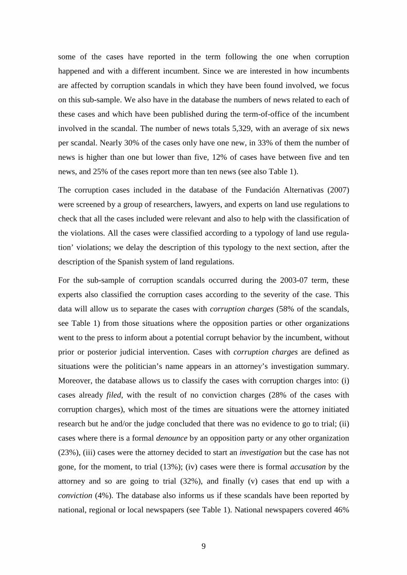
[Insert Figure 1]
The situation started to change after 1995, with the switch in the housing market
situation, but did not explode until 1999. Figure 1 displays the 1991-2007 evolution of
the corruption episodes included in the database described in the previous section. The
grey line in Figure 1 shows the evolution in the number of municipalities with at least
one corruption case, defined by year of occurrence of the corruption act. Before 1999,
there were just 46 corrupt municipalities. The number jumped from 16 in 1999 (and just
4 of them before the June 1999 local elections) to 86 in 2000, and the level of corruption
never reverted after this date and experienced another big surge in 2006, where the
number of corrupt municipalities jumped to 180. The black line in Figure 1 shows the
evolution in the number of corruption scandals, defined as the cases that were revealed

11
through media news during the term of office and which can be attributed to the
incumbent party during this term. Over the 1999-2007 period, 666 corruption cases
were reported by the media during the term-of-office in which the party responsible for
the corruption act was the incumbent. This represents roughly a 94% of the cases
occurred through the period. Despite the delay in reporting, apparent from the fact that
there are always more corruption cases than scandals, the pattern of both series is very
similar. This suggest that corruption could have been an issue for the first time in the
2003 local elections, since before 1999 there were some cases but virtually no scandals,
reporting not beginning till 2000. It also seems that the surge before the 2007 local
elections was much more intense than the one before 2003.
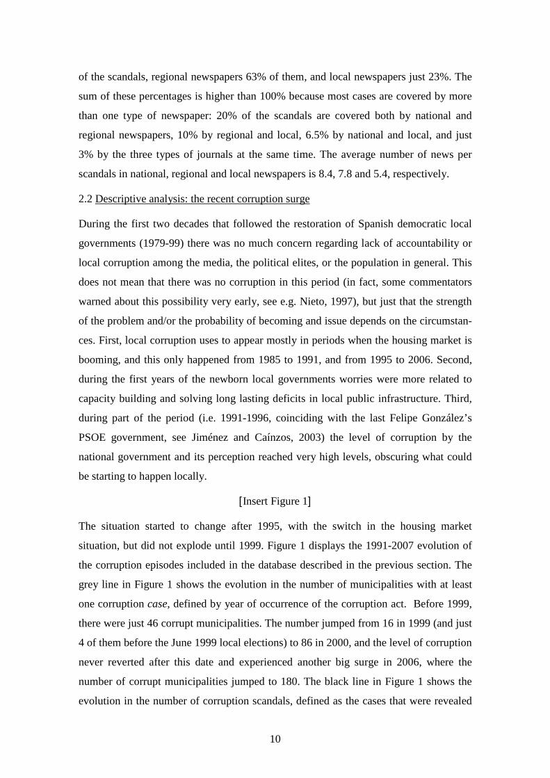
[Insert Figures 2 and 3]
Figure 2 displays the evolution in the number of scandals vs. the evolution in the
number of news published regarding these scandals. Both series show a very similar
evolution. Note, however, that despite the decrease in the number of cases in 2003, the
number of news also peaks during this election year. This behavior can be seen more
clearly in Figure 3, which compares the evolution in number of scandals vs. news per
scandal. News per scandal rose through the period, meaning that the reporting intensity
increased over time, with peaks in 2003 and 2006 that can be explained by the proxi-
mity of the 2003 and 2007 local elections. The rise before 2007 seems steeper than the
one during the month prior to the 2003 elections.
[Insert Figure 4]
How was this perceived by the voters? Figure 4 shows the evolution of the percent
people than cite ‘corruption and fraud’ as one of the three worst problems of the country
during the period that goes from September 2001 to December 2008 (Source: CIS
Barometer, several years). Note that the negative perception of corruption jumped just
around the 2003 elections and before the 2007 ones. The 2003 jump is a very sudden
one, reflecting the fact that corruption was relatively low since recently, and news did
not reach the general public until its use as an issue during the political campaign. Prior
to this jump, the worries about corruption were dropping since 2001, perhaps reflecting
a vanishing impact of the 2000’s cases. What happened before the 2007 elections is a
little different, in the sense that corruption worries jumped up earlier in 2006, coinciding
with the surge of scandals and news documented in Figures 1 to 3, and reached high

12
peaks in three of the surveys undertook before the May 2007 local elections. This
evidence, coupled with the one related to the evolution in the number of scandals,
suggest that the impact of corruption scandals on the vote should be expected to be
stronger in the 2007 than in the 2003 elections, although it is also plausible that some
punishment had yet appeared.
[Insert Figure 5]
What about prior elections? Figure 1 documents nearly no cases before the 1995 elec-
tions and just a few cases before the 1999 ones, and no corruption scandals before the
1999 elections. To reinforce this idea, Figure 5 plots the percent of people saying that
‘politicians and parties’ are one the three worst problems of the country during the
period January-1995 to December-200811. Note that the percent of ‘yes’ answers to this
question dropped abruptly from a very high level (i.e. 22% of the population) before the
general elections held in March-1996 to just a 2% before the June-1999 local elections.
The high level of corruption awareness before 1996 reflects the corruption scandals that
affected the last PSOE government led by Felipe González. Corruption was an impor-
tant issue during the 1996 electoral campaign but progressively disappeared from the
public arena after the socialists were ousted from government. Note also that the percent
of people citing politicians as a problem continued to drop after the 1999 local elections,
and only started to peak in mid-2000, coinciding with the first corruption scandals docu-
mented in Figure 1. This reinforces our idea that corruption in local governments should
have not been perceived as a problem prior to the 1999 elections.
2.3 Corruption causes: land use regulations
Spanish commentators have provided several explanations for the recent corruption
surge in local governments. Some claim that Spanish voters are especially tolerant with
corruption, due to cultural and/or historical motives (see Fundación Alternativas, 2008,
for a discussion). Others speak about the low levels of transparency in local decision-
making (Transparency International, 2007) or about the hidden interests of the main
political parties, which are so soft with corrupt behavior because part of the money
collected end up funding electoral campaigns (Nieto, 1997). However, the fact that the
11 The other question, more directly related to ‘corruption and fraud’, disappeared from the survey for the period July-1999 to September-2001, so we are not able to plot it for this wider period. Note, however, that Figure 4 also displays peaks close to the 2003 and 2007 elections, suggesting that people responds in a similar way to both questions.

13
majority of local corruption scandals are related to bribes received in exchange of
amendments in land use plans, suggests that the specific traits of this type of regulations
could have played a major role in Spain, specially when combined with a real state
shock of an unprecedented dimension.
Land use regulations in Spain adhere to an extremely interventionist and highly rigid
system (Riera et al., 1991; Riera, 2000). A key characteristic is that, although an
individual might own the land, the government is empowered to control and implement
all processes of urban development. Landowners are not permitted to develop their land
without the prior agreement of the local administration. It is not simply that they need a
building license (which is in most cases automatically granted): before reaching this
step, the government must have declared the land ‘developable’ and defined most preci-
sely the conditions for such development. The main tool employed by the government
for doing this is its urban plan. Therefore, town planning in Spain is essentially a
municipal responsibility, but as there are more than 8,000 municipalities nationwide, the
system is highly fragmented (as in the US)12. Municipalities draw up a ‘General Plan’,
which provides a three-way land classification: built-up land, developable land (the
areas of the community where future development is allowed), and non-developable
land (the rest of the territory –agrarian and other uses, where the development process
is strictly prohibited, at least until a new plan is approved). The ‘General Plan’ includes
very detailed regulations regarding many other aspects: land zoning (residential,
commercial, industrial), the maximum floor-to-area ratio for each plot, the reservation
of land for streets, green spaces and public facilities, etc.
The existence of a ‘development border’, a line between plots of land on which
developers are allowed to build and plots where development is banned, is a key feature
of Spain’s land regulation system. In periods of high demand this border creates a rent
differential which might fuel the bribes developers are willing to pay to local politicians
in exchange for shifting this border to their advantage13 , 14. The higher this rent
12 However, the powers are partly shared with regional governments. Thus while the municipa-lities define the plan and control its implementation, the regional government must first accept the plan and ensure that all legal regulations are adhered to. Other responsibilities of the regional government include the design of supra-municipal plans and the declaration of certain areas as protected zones. Yet, in practice, the use of regional power to restrict local land use policies has been quite infrequent (Riera, 2000). 13 See Brueckner (1999), for a simple exposition of the effects of these development borders. See also Hannah et al. (1993), Green et al.(1994) and Son and Kyung (1998) for analysis of the effects of this type of land use regulation.

14
differential, the stronger the incentives for developers to provide bribes to local officials
in exchange of a displacement of the border, which converts more land from rural to
potentially developable (see Solé-Ollé and Viladecans, 201015). The rent differential is
higher the lower is the amount of vacant land already available for building. And the
vacant land is higher in part because past governments were not really against develop-
ment and in part just as a result of past forecasting errors (a lot of land was converted
during past housing booms, but the cycle turned into a bust and the forecasted building
projects never materialized). With more vacant land, it is less probable that developers
want to offer bribes to change other components of the plan (e.g. push for higher buil-
ding densities in already built up places or for permits in places previously banned to
construction, as parks), since they have the alternative of building in vacant land
without paying bribes. Moreover, places with less vacant land are probably also places
with less regulatory stringency in general (referred to planning dimensions other than
the extensive use of land), and this suggest also that in this places starting a construction
project is in general more easy, requiring the effort in bribing local officials.
In addition to decision-making discretionarity, lack of transparency and demo-
cratic participation channels in planning decisions are also a big concern in Spain. In
theory, the ‘General Plan’ has a duration of eight years, but the land classification can
be quite readily modified by a majority vote in the municipal council. The amendment
plan, known as a ‘Partial Plan’, is also a legally binding document. A number of
participation and transparency requirements apply to facilitate scrutiny by the residents,
who can seek to change the document if they so wish. These requirements are stricter in
the case of the initial introduction of the ‘General Plan’, but here the real degree of
transparency of the system is very much dependent on the will of local politicians. To
implement the plan the local officials can resort to a variety of means to introduce the
desired amendments, without these changes having to come under much scrutiny from
residents or the media. This is the case, for example, of the contractual arrangements
made between local governments and developers (the so-called ‘Convenios Urbanís-
ticos’), which are permitted under Spanish law. Such contracts might modify the urban
14 The ideas that monopoly control of regulations by the government create rents and that rents provide incentives for corrupt behavior can be found in many prominent works on corruption (see, e.g. Rose-Ackerman, 1978 and Ades and Di Tella, 1998). 15 This is one of the few papers modeling political decision of urban growth boundaries as arising from the interaction of local officials that care about re-lection and a developers lobby. Other papers with lobbies bribing local officials in exchange reduction of land use regulatory intensity are Glaeser et al. (2005) and Hilbert and Robert-Nicoud (2010).

15
status of a plot, its floor-to-area ratio, or renegotiate the terms of developers’ payments
to the city budget.
Many of the recent Spanish stories about corruption are consistent with these
explanations. There are plenty of cases related to local officials unduly allowing huge
amounts of land to be developed, amending the plan in order to allow for higher
construction densities in already developed land, or allowing building in places were the
previous plan didn’t allow it (e.g. Martin Mateo, 2007, and Fundación Alternativas,
2007). Many of the cases are also related to not very visible contracts between
developers and the city council, as a recent report has identified (Transparency
International, 2007). Finally, in some of the cases corruption arises because land owned
by the municipality is sold at below market prices or because payments made by
developers to pay for basic infrastructures are in practice less than the ones required by
the law16,17.
Our database provides information regarding which is the type of land planning
violation incurred by local politicians in each corruption scandal. The violations are
classified as: (i) Plan design (23% of the scandals, see Table 1): Classification of land
as developable when its legal characteristics do not allow for it, or bribe-taking related
to land classification even if the decision has been approved by the city council follo-
wing established procedures. (ii) Plan implementation (32%): Modifications of land
classification of an already approved plan, cases related to elimination of green areas or
allowing for higher densities abounding. This category also includes corruption related
contracts between developers and the city council (‘Convenios Urbanísticos’), often
involving barters of land plots that go against the interest of the citizens. (iii) Plan
enforcement (10%): Building allowed by the local council in places not allowed by the
plan or by other regulations or judicial decisions. This category includes cases of
granting building licenses in non-developable places or inaction against illegal
construction. (iv) Public land management (33%): Public land sold at below the market
price or bartered for a less worthy plot. And (v) Environmental violations (21%): Local
16 This type of corruption is similar to the one identifies by Cai et al. (2009) in the case of Chinese land auctions. 17 Under Spanish law, developers have the obligation to pay for basic infrastructures (streets, lighting, sewerage and water systems), and to donate land to local council with a value equal to than 10% (in some regions this goes up to 25%) of the value of converted land plots. If written in a contract (one of these ‘Convenios’), the payment can be made in money instead than in land, but if made in land the municipality can decide either to retain the land (e.g. to build facilities, as schools or hospitals) or to auction it.

16
planning decision contrary to higher level environmental protection legislation. Note
that sum of the percentages is higher than 100%; this occurs because some corruption
cases have more than one type of violation at the same time. For example, corruption
scandals related to Public land management always go together with some other
violation (the average is two additional violations), the most prevalent combination
being with violations related either to Plan design (15% of the times) or to Plan
implementation (22% of the times). This also occurs with violations related with Plan
implementation (with 1.4 additional violations on average) which go hand in hand with
violations in Plan design (17% of the times) and with Environmental violations (13% of
the times). Other types of violations as Plan enforcement use to occur in isolation (only
0.2 additional violations).
3. Empirical analysis
3.1 Dependent variable, period and sample
The purpose of the analysis is to estimate the effect of reported corruption scandals
affecting the incumbent during a given term-of-office on her vote results at the
following local elections. We analyze the vote for the incumbent party or parties and not
the vote for specific candidates, since our database does not provide this information.
However, just few of the candidates affected by corruption scandals decided not to run
or were forced by the parties to retire. For example, in the 2007 elections just fifteen
corrupt candidates decided not to run again (see Fundación Alternativas, 2008)18,19. The
2007 results (available upon request) do not change if we exclude these municipalities
from the analysis. We don’t have information of candidate retirement for the 2003 elec-
tions, but the picture should not be very different.
Since a substantial percent of municipalities are governed by coalitions (34% and 32%
in the 1999-2003 and 2003-07 terms, respectively), our dependent variable has been
constructed as the sum of votes over all the parties in the government team (including
the party of the mayor, which is the most voted one in the vast majority of cases, and the
18 This report speculates about the causes of the decision to not retire, suggesting that by accepting retirement the parties would have implicitly accepting there has been corruption. Also, in some cases, the party lacks the disciplining devices to impede any candidate to go to the elections with a different brand, in which case it could cause vote losses to the party candidate. 19 We don’t have any information about the decision to retire in municipalities belonging to the non-corrupt group, but it would very strange that this behavior was more frequent here than in the corrupt one.

17
partner parties) over the number of votes to parties (in and out the government). The
average incumbent’s vote share is around 55%, both in 2003 and 2007 and both for
majority parties and coalitions. In the case of coalitions, the average vote share of the
mayor’s party is 40% and that of the partners is 15%. Data needed to construct this
variable comes from the Spanish Ministries of Interior and Public Administration (see
Table 2 for definitions and sources of the variables).
We focus on the incumbent’s vote share in the two local elections that could have been
affected by the surge in corruption scandals, i.e. those of 2007 and 2003. As reported in
the previous section, it seems that media and voters concerns about corruption reached a
highest peak before the 2007 elections, the effect being less clear in 2003 and sure non-
existent in the prior ones (1999 and 1995). Because of this we will pay more attention to
the analysis of the 2007 elections, albeit also presented some results for the 2003 ones.
In any case, we believe that the time evolution of the phenomenon justifies a separated
treatment of the two elections.
[Insert Table 2]
In our analysis we will compare the municipalities that experienced a corruption scandal
for the first time during the term we are analyzing (either the 1999-2003 or the 2003-07)
with the municipalities that did not experience a corruption scandal in the previous
terms (i.e. 1995-99 and 1999-2003 in the case of the 2007 elections, and 1995-99 in the
case of the 2003 ones). For the 2007 elections, the ‘treated’ group has 294 municipa-
lities (83 municipalities experienced corruption during this term but also in the previous
one, for a total of 377 ‘corrupt’ municipalities). The resulting number of observations in
the 2007 elections’ control group is 4360 (for a total of 4649 observations, after adding
the 294 treated municipalities)20.
The reason for dropping these observations from the treated group is that corruption
might have a different impact on the vote after been also experienced in the previous
term, and this might also depend on whether the incumbent was ousted or not. The
motive for dropping the previously corrupt municipalities from the control group is that
20 Spain has more than 8,000 municipalities, but most of them are quite small. The control group is smaller than this number just because of data gathering problems. We believe that our control group is fairly representative of the population, since it includes the vast majority of municipalities bigger than 5,000 inhabitants and some checks done with the remaining part of the sample show that the average values in the sample and the population (for the few variables which are available in both cases) are really similar.

18
corruption scandals might have effect not only on the election before which the infor-
mation has been revealed, but also in subsequent ones. We believe all these cases
deserve a separate analysis, which we will also report. In the 2003 analysis, we are able
to retain all 4732 observations (289 ‘treated’ and 4443 ‘controls’), basically because our
main database does not record corruption cases prior to 1999.
3.2 Empirical strategy
Estimating the effects of corruption scandals on the incumbent’s votes is tricky because
corruption is more probably to occur in places where the popularity of the incumbent is
high. Failure to account for this will bias negatively the estimates. In this section, we
explain how we deal with this problem with three different methods: (i) OLS with
controls, (ii) ‘Difference-in-differences’, and (iii) Instrumetnal variables.
OLS with controls. The most quantitatively relevant popularity differences across
municipalities in Spain come either from voters’ historical attachment to some political
parties (Solé-Ollé and Viladecans, 2010) or from national and/or regional party tide
effects (Bosch and Solé-Ollé, 2006). Differences in ideological attachments to parties
can be washed out if one has access to data from more than one election. With this
purpose, we begin by defining our dependent variable as the increase in the incumbent
party vote share between two consecutive elections (see Table 2 for statistical sources),
which can be expressed as:
tikjt
tikjt
tikjt 1VV∆V −−= (1)
Where V is the vote share, the super-index t indicates that votes correspond to the party
which is the incumbent during the term preceding election t∈ [1,2], and sub-index i, j
and t and t-1 indicate that votes were obtained in municipality i, belonging to region k,
by party j, and at the electoral contests t and t-1. By using the vote share between two
elections we are able to get rid of any influence of the vote share of a party that is muni-
cipality-specific.
Popularity differences arising from national and/or regional party tide effects can be
controlled in an OLS estimation by including party-election dummies in a cross-sectio-
nal regression for each election. The estimated equation would look like:
itititkjttikjt ZC εγβα +++= d∆V (2)

19
Where kjtα are region × party × election fixed effects, and its inclusion is justified by
the fact that local elections in Spain are partly bi-elections of the regional and national
ones. This means that when the popularity of a party goes down nationally, so it does
his vote share at the local elections (see, e.g. Bosch and Solé-Ollé, 2006). These tide
effects are often of a different intensity in different regions, so we allow these effects to
differ across regions and parties, for a given election. itCd is a dummy equal to one is
there has been a corruption scandal in the municipality during the term-of-office
preceding election t. We will also estimate the model with alternative measures of
corruption (e.g. numbers of news), but for easiness of exposition we refer only to the
corruption scandal dummy in this section. itZ is a vector of controls, including: popula-
tion size dummies, property tax increase, increase in current spending, investment and
debt, growth in population and unemployment, and coalition dummy and party frag-
mentation index (see Table 2 for definitions and sources). itε is a random error term
with the habitual properties.
Difference-in-differences (DD). There are, however, some differences in popularity that
are not incumbent-specific but municipality-specific. For example, in some places the
incumbency advantage might be higher than in others (i.e. in some places there is a
higher probability that an incumbent that obtained a given vote share in the past elec-
tions will be ousted from government). If these differences are constant in time, they
can be accounted for by the inclusion of a municipality fixed effect in equation (2):
itititkjtitikjt ZC εγβαα ++++= d∆V (3)
Where iα is a municipality fixed effect. However, to get rid of the fixed effect, one has
to be able to access to data of at least another election. Since we also have information
from the 1999 and 1995 local elections, we will be able to estimate expression (3) with
two cross-sections for each election. For the 2007 local elections, we have a panel with
the 2003-07 and 1999-2003 cross-sections. Note, moreover, that by definition of the
‘control group’ (see previous section), itCd =0 for all the municipalities in 1999-2003.
For the 2003 local elections we have a panel with the 1999-2003 and 1995-99 cross-
sections. Given that there are no corruption scandals in our database for the period
1995-99, itCd is also zero for all the municipalities in this cross section. In this context,
the interpretation of the ‘difference-in-differences’ estimates is that β is the effect over

20
the increase of the incumbents’ vote share between two consecutive elections of
experiencing a corruption scandal for the first time, compared with municipalities that
did not had this experience in the past. Obviously, we also control here for region ×
party × election fixed effects, so this effect is measured with respect to the increase of
the incumbent’s vote share in municipalities of the same region and controlled by the
same party.
Instrumental variables. However, the DD method is not able to deal with the possibility
of specific municipality×term popularity shocks (beyond those picked up by the region
×party effects×election effects). A way to address this potential problem is to use an
Instru-mental Variables estimator. The instruments for itCd will be the interaction
between measures of building demand shocks faced by the municipality each term and
the inver-se of the amount of vacant land it had at the beginning of the term. The idea
behind this instrument is that the willingness of developers to offer bribes in exchange
of amend-ments in land use plans will be high if two conditions concur at the same time:
a strong demand for building in the locality + scarcity of planned land where to build
(i.e. vacant land); if there is plenty of local land, strong demand pressures are irrelevant,
since the developer can build anywhere without having to pay bribes; similarly, if there
are no demand pressures, scarcity of local land does not spur bribe-giving, since the
developer will not obtain any gain from doing it.
The demand shock variables are the dummies beachi (=1 if the municipality has a
beach)21 and urbani (=1 if the municipality belongs to an urban area), which have been
shown in previous analysis as powerful drivers of local development during this period
(Solé-Ollé and Viladecans, 2010). A simple visual inspection to the map of corruption
cases corroborates the impression that these dummies might have explanatory capacity
(see Figure 6). We also tried with interactions between these variables and with others
(e.g. distance to the beach, distance to the CBD, percent sunny and freezing days,
interactions between the weather variables and beach and urban, and different beach
21 Other papers have suggested that geographical and climate traits might be the ultimate facilitator of corruption. For example, in Leeson and Sobel (2008), the location in flooding areas lead to a windfall in relief transfers that generate corruption (see also Leite and Weidman, 1999). Our story is not so different: a huge and exogenous demand for building second-home houses in coastal municipalities (led basically by low interest rates and growing income in Spain and the rest of Europe) created a big rent differential between urban and rural land in unprepared municipalities (those with a low amount of vacant land) that fuelled corruption.

21
variables for each of the major Spanish coastal sectors, different urban areas depending
on the size of the central city), but the explanatory capacity of the instruments did not
improve much. These three variables have been multiplied by the average extra growth
of these types of municipalities during each term, ∆beacht and ∆urbant. This extra
growth has been obtained after estimating an auxiliary regression between the growth
rate of the build-up land area by municipality and term, and the interaction of the two
variables with each of the term dummies22. Finally, note that the instrument is not just
being on the beach or on an urban area, but the interaction with the time variation of
construction in these places and with the amount of vacant land available at the
beginning of the each term of office (i.e. beachi× ∆beacht/vacantit and urbani ×∆urbant/
vacantit). This means, first, that systematic differences between beach and urban
municipalities and other places are already captured by the fixed effects in the DD
regression and, second, that we don't need to assume that each of these variables alone
is uncorrelated with any specific trend. We only need to assume that the intensification
of demand pressures from one term to the following in beach and urban places with
shortage of vacant land is not correlated with any such trend.
However, our confidence on the interacted instruments is improved by the fact that there
is some evidence that suggests that even the beach, urban and vacant variables need not
being correlated with any trend in electoral competition. First, we can show that places
that have grown more during the period 1979-2007 didn’t experiment any significant
variation in electoral competition. With this purpose in mind, we have computed the
Pedersen index of vote volatility (Pedersen, 1979)23 for the Spanish local elections of
1986, 1991, 1995 and 2007 (which define periods of boom and bust in the housing
market), using provincial-level data that election and on the two previous ones. It turns
out that the correlation between the increase in the volatility index and the growth rate
of the housing stock (IVIE, 2008) is very low and not statistically significant24. We also
22 This regression returned the following coefficients (p-values in parenthesis) for the interact-tions of the beach variable with the 1995-99, 1999-03, and 2003-07 dummies: 0.10 (0.052), 0.18 (0.021) & 0.28 (0.003). The same coefficients for the urban dummy are 0.05 (0.078), 0.15 (0.058) & 0.25 (0.001). It is evident that the differential between the growth of beach and urban municipalities and other places in Spain grew as the housing boom intensified. 23 This index is computed as the net percentage of voters who changed their vote between parties from one election to the following one and summed over elections. 24 The correlation between these two variables pooling the 1986-91, 1991-95 and 1995-2007 periods together is just -0.024 (p-value = 0.302). The correlations for each of the three periods are also not statistically significant.

22
compute the growth in that index in coastal and non-coastal and in urban and non-urban
provinces, without finding any meaningful difference.
Second, there is some evidence that shortage of developable land is a quite random out-
come: a municipality has too much (too few) developable land if it made mistakes in the
past and forecasted a too high (too low) demand shock. One could argue that these mis-
takes are not random, municipalities growing more/less making systematically bigger or
smaller mistakes. This could pose some treat to out estimates if omitted growth is also
correlated with vote results. This seems not being the case: the correlation between
vacant land at the beginning of each term and growth during the previous term (using
here the growth in build-up area at the municipality level, same source than for vacant
land, see Table 1) is also very low and not statistically significant25.
Finally, we have to say that we also use our instruments in estimations that do not rely
on the DD method, but just on estimation by OLS with controls. We still rely on the
interacted instruments in this case, but including the non-interacted variables as further
controls in the equation. The identification assumption is now that higher demand
pressures in beach and urban places with shortage of vacant land are not correlated with
the omitted level of political competition (i.e. picked in the DD case by municipality
fixed effects). Since, as we showed above, vacant land is quite a random outcome, this
assumption will probably hold. Also, we can show that the Pedersen volatility index is
not correlated at the provincial level either with the growth rate of the housing stock
(using the same period than before) or with being on the beach, although it seems that
urban municipal-lities do if fact have more volatile elections. So, we should interpret
these results with some caution, and look at how the results change when the urban
instrument is dropped. In any case, the availability of more than one instrument will
allow computing over-identification tests, at least in the cases where we only have one
endogenous variable.
3.3 Empirical results
Tables 3 to 9 present the results of the estimation of the effects of corruption scandals
on incumbent’s votes. Table 3 presents the OLS and DD results for the 2007 elections
25 The correlation between vacant land in 2007 and growth in built-up area during 2003-07 is just 0.0231 (p-value = 0.298) and the correlation between vacant land in 2003 and growth during 1999-2003 is -0.001 (p-value: 0.6923).

23
using just the dC dummy as a measure of corruption. Table 4 shows the DD results for
the 2007 elections when adding to the equation several additional measures based on the
number of news. Table 5 presents the DD results exploring the effects of different types
of corruption scandals, as classified either according to the type of land-use regulation
violation or according to the severity of the case. Table 6 displays the IV results also for
the 2007 elections. Table 7 presents the a summary of the DD and IV results for the
2003 elections. Tables 8 and 9 show IV results for sub-samples of municipalities and
the 2007 elections.
Main OLS and DD results: 2007 elections. Columns (i) to (iii) of Table 3 show the OLS
results regarding the effect of having a corruption scandal (dC=1) when adding: (i) just
election fixed effects (i.e. a constant plus a 2007 dummy), (ii) election fixed effects and
control variables, (iii) Region ×party×election fixed effects and additional control varia-
bles. Columns (iv) to (vi) show the DD results (i.e. with municipality fixed effects to the
equation), consecutively adding the same sets of controls than in the OLS case. The
OLS estimates with no controls suggest that a corruption scandal detracts just a tiny
1.4% of the incumbent’s vote. This number jumps to 2.4% and 3% when adding the
different sets of controls. The DD results with no additional controls are higher than the
OLS ones (2.2%) but they are fairly similar when all the controls are included in the
equation (3.3% vs 3% in the OLS case). Region ×party× election fixed effects seem to
do a good job in controlling omitted popularity, especially in the specifications without
municipality fixed effects.
[Insert Table 3]
Additional DD results: number of news. Table 4 presents the DD results when adding to
the equation other measures based on the number of news. Columns (i) to (iv) explore
the effects of including counts of news, while columns (v) to (vii) analyze the effects of
news published in different types of newspapers (national, regional or local). The results
in columns (i) and (ii) show that both having an scandal and the intensity of newspaper
coverage of this scandal matter. The estimates suggest that an incumbent facing the
average scandal in terms of number of news (eight during the 2003-07 term) will lose
2.7% of the vote after the first new is published and an additional 1.6% after all these
news accumulated, for a total of a 4.3% loss. Column (iii) searches for a possible non-
linear effect of the number of news, using dummies identifying thresholds of more than

24
five, ten and twenty news. The base category is a corruption case with less than six
news. It turns out that having more than five news (but less than ten) does not make any
difference, but that having more than ten news does cause a significant additional vote
loss. Having more than twenty news does not make any difference, once an incumbent
has received more than ten26. It seems therefore that the ten news threshold is the one
that better defines a scandal a having a substantial cove-rage by the press. This means
that for the 25% of scandals in the sample that have more than ten news, the
incumbent’s vote loss can be much higher than for the rest, going up to 8.8% (i.e.
2.7%+6.2%, see column (iv)). This could be due to the fact that only the more serious
cases have this coverage or to the press coverage being more intense in some
municipalities than in others27.
Columns (v) to (vii) display the results obtained when we split the corruption scandals
and news according to the type of newspapers (national, regional and local). In column
(v), the base category is corruption scandals which have been reported by regional
newspapers. The results suggest that scandals reported also by the national or by the
local press don’t have a stronger effect on the incumbent’s vote than the ones reported
only by regional newspapers. In column (vi) news reported by national newspapers
don’t have a stronger effect than the regional ones, and local news about corruption are
actually good for the incumbent. Column (vi) combines the more than ten news
dummies with thresholds for national and local news. Again, it turns out that scandals
substantially covered by national and/or regional newspapers but not by the local media
detract a lot of votes from the incumbent (12.1%=2.4%+9.7%). If the scandal is also
covered by the local media this effect is much lower (5.3%=9.5%-4.4%), although still
higher than if the scandal is not widely followed by any kind of newspapers (2.4%).
These results could be due to the fact that newspaper competition is probably very low
at the local level. Most of the times, there is just one newspaper at the local level, and it
uses to be partly funded by the local council. We speculate that government capture of
26 We investigated a finer classification, but obtained very similar results 27 To try to disentangle these two effects, we performed an additional analysis. We interacted the ten news dummy with the number of newspapers sold per capita at the provincial level (we lack local information on newspapers). The interaction was not statistically significant, suggesting that our results are driving by the differential effect of more serious corruption violations on the incumbent’s vote.

25
local media is quite plausible in these cases. Overall, the results of this table suggest
that the role of the media in promoting accountability is quite important; more sever
corruption scandals being more reported and causing higher vote losses because of this.
Regional newspapers seem to play a role as relevant as the one of national newspapers,
but this is not the case of local news-papers, with some results suggesting that they can
even have a negative effect on the promotion of local government accountability. More
investigation is clearly needed to understand these results.
[Insert Table 4]
Additional DD results: type of scandal and severity. Table 5 presents the DD results
when adding to the equation the dummies which classify the corruption scandals accor-
ding to type of land-use regulation violations (Columns i to iv) and severity (Columns v
to viii). The results relating to the type of land-use regulations suggest that this does not
matter much. One exception to this is violations related to Public land management, i.e.
those in which a local official forgave developers to satisfy some fees or sell public land
at below-market prices. Column (iv) suggest that punishment goes up by 4% in these
cases (albeit the coefficient is only statistically significant at the 10% level), punishment
in widely reported cases involved this type of violations causing a vote loss of around
11% (11.2%=2.2%+5%+4%). The reason this type of violations is more punished than
the others is that it is perhaps easy for the voters to understand the kind of loss caused to
the community; note that in this case, the violation means that less money will enter the
city’s coffers, while in many of the other cases the loss is only in terms of over-building
in places were the voters (or some higher layer of government) though development
should be banned.
[Insert Table 5]
Columns (v) to (viii) report the results related to the severity of the corruption case. The
results suggest that cases formal accusation by the attorney (so, cases that go to trial)
cause a substantial vote loss (and additional 5%) over cases without any kind of charge
(the base category, picked up by the dC dummy). Conviction also causes an additional
4% loss, and cases that are under investigation (but that did not reach any of these two
previous levels) detract an additional 1.6% voter share. Note that all these cases exclude
one each other. An interesting result is that cases were there is just a denounce by the

26
opposition do not detract votes (in fact, the coefficient is positive, though not statisti-
cally significant, and cases already filed (and which did not end with a conviction)
actually report additional votes for the charged incumbent (around 4%). These results
suggest voters do not consider that cases of corruption raised by the opposition
(denounce) are really credible. A filed case is also interpreted as direct evidence that the
charge was motivated by the intention to harm the opponent. Note also from the table
that, once we have accounted for the severity of the scandal, the effect of a scandal
without charges of corruption (picked up by the dC dummy) is smaller (1.3% in
columns vii and viii) and only statistically significant at the 10% level. The last column
(viii) presents average results for municipalities with some type of corruption charge,
taking into account only those which are alive (i.e. excluding the filed cases). The result
suggest that electoral punishment is different depending on the incumbent being
charged or not and also (as before) on press coverage. Scandals with formal charges and
wide press coverage cause a substantial vote loss (10.8%=1.3%+4%+5.4%). Scandals
already filed and with wide coverage cause just a vote loss of 1.3%, and this turns into a
vote gain is there is no such wide press coverage (2.8%=4.1%-1.3%).
Main IV results: 2007 elections. Table 6 displays the main IV results. Given that we
only have two reliable instruments, we limit the analysis to equations including to cor-
ruption measures at the same time, so we will not be able to report results so detailed
that in the DD case. The first two columns report the results when including only the
corruption dummy (dC), with just Municipality and Election fixed effects (column i) and
with Regional × Party fixed effects and Additional controls (column ii). Columns (iii)
and (iv) repeat these estimations substituting the corruption dummy by the number of
corruption news, columns (v) and (vi) use both variables at the same time, and columns
(vii) and (viii) combine the corruption dummy with the dummy identifying situation
with more than ten news. The results suggest that a corruption scandal detracts around
5% of the vote (column ii), and the estimate is higher than the DD one (which was
around 3%). One corruption new detracts 1% of the vote (column iv), five times more
than in the DD analysis (see Table 4), although now the coefficient is only statistically
significant at the 10% level. This means that the average incumbent will loss 8% of the
vote. Wide coverage of the scandal detracts 12% of the vote (column viii), compared to
the 6% obtained in the DD analysis, although here the statistical significance of the
coefficient is also limited to the 10% level. Overall, the IV estimates seem to be higher

27
than the DD ones, but also noisier. In any case, we have to say that the instruments
performed well, in the sense that they both overcome the weak instruments tests28 and
the over-identification tests (presented at the bottom of the table). Additionally, the
negative OLS bias is consistent with the idea that there are some omitted municipality
and term specific popularity factors.
[Insert Table 6]
Main DD and IV results: 2003 elections. Table 7 present a summary of the main results
obtained for the 2003 local elections. Columns (i) to (iv) present the DD results and
columns (v) to (viii) the IV ones. Note that both the DD and the IV estimates are much
lower than the ones for the 2007 elections. For example, the impact of a corruption
scandal, as estimated by DD, is now 1.7%, lower than the 3.3% of the 2007 elections.
The IV estimate is 3.3%, also lower than the 4.8% of 2007. The impact of news and of
widely reported scandals (more than ten news) is also lower in this case. Moreover,
most of the coefficients are not statistically significant or are significant just at the 10%
level. The general conclusion is, therefore, that there evidence of punishment of corrupt
incumbents is less clear in the 2003 elections, albeit the results suggest that something is
going on. The evolution of corruption cases and public perceptions of corruption (see
section two) explain why this might have been the case.
[Insert Table 7]
Heterogeneous effects. The literature on the effects of corruption on the vote suggest
that punishment of corrupt acts can be substantial only if the appropriate circumstances
concur (see Jiménez and Caínzos, 2004, for a review). For voters to decide to change
their vote in response to a corruption scandal some conditions have to hold: (i) they
have to be informed about the scandal, which requires that the media decides to report it,
(ii) they have to believe that news are reporting real corruption, and not just partisan
accusations deemed to erode the support of the opponent, (iii) they have to be able to
clearly identify the candidate, or at least the party, which is responsible of the corrupt
28Both instruments are relevant in the first stage. For example, the first-stage for column (ii) is:
dC = 0.334×Beach/vacant + 0.173 ×Urban/vacant + Region×Party effects + Additional controls. (2.38)** (3.73)***
t-values in paréntesis, ** & *** =statistically significant at the 5% and 1% levels. The full set of first-stage regressions are available upone request.

28
act, (iv) they need to have an alternative, meaning that they should be willing to vote for
another party or to abstain, (v) they should have a negative evaluation of corruption,
which means that there should not obtain other significant benefits associated to the
corrupt act. The results presented in this paper up to now provide some evidence that the
first two conditions are relevant: the more press coverage and the more convinced are
voters about the incumbent being guilty (thanks to judicial intervention), there higher
the chances of punishment; the higher the suspicion of partisan use of the scandal, the
less punishment.
Evidence on condition (iii) can be found by looking at how voters evaluate corruption in
single-party vs. coalition governments. The ‘clarity of responsibility’ hypothesis (Powel
and Whitten, 1993) states that voters are less able to attribute responsibility to the in-
cumbent in the case of coalition governments. Sometimes, when a corruption scandal
appears, it is quite clear who are the officials involved and to which parties they belong.
In other occasions, even if some officials belonging to one party are charged, there are
some doubts regarding the degree of diffusion of corruption inside the city council, to
other officials and to other parties. An in other occasions simply officials of all the par-
ties are involved in the scandal. We don’t have information regarding the parties of the
officials with corruption charges in coalition governments (this would have required a
specific search that was not done), but we can look at how voters punish the single
parties vs. coalitions, and in coalitions whether they punish the party of the mayor or the
partners.
Evidence on condition (iv) can be obtained by looking at how voters punish incumbents
belonging to different parties. In Spain, left-wing voters tend to have more outside
options than right-wing ones (e.g. PSOE voters can vote for the communist party or for
other left-wing regional parties, while PP voters have no alternative in most parts of the
country) and they also use to abstain more when dissatisfied with their party. Of course,
evidence that some parties are punished harder than other could also tell us about the
tolerance to corruption of people voting for this party (condition v). Additio-nal
evidence on (v) could be gauged by looking at municipalities in which many voters
obtain side benefits related to corruption in land-use regulations. For example, in some
municipalities, development is justified as a means of providing better economic oppor-
tunities to the residents. Excessive development (i.e. the one that destroys natural re-

29
sources, like forests and nice beaches) will probably not bring much prosperity over the
long run. However, if a substantial percent of the population is unemployed, the long-
run probably does not matter a lot. This effect could be reinforced in places with a high
percent of jobs in the construction industry, and in places with low job mobility (i.e. in
places with a low percentage of out-commuting). Also, places with a high percent of
homeowners are more likely to punish corruption, since the urban economics literature
suggests that they are especially opposed to growth that could affect negatively both the
quality of life and the value of the houses (see e.g. Fischel, 2001). We will analyze whe-
ther electoral punishment of corrupt acts is stronger or not in these places.
Table 8 presents the IV results obtained when splitting the sample into left and right-
wing parties (see Table 1 for definitions) and one party vs. coalitions. The first two
columns compare left with right parties. Punishment seem to be stronger in the case of
left-wing parties, a fact that can be found both in the literature of corruption (Peters and
Welch, 1980) and on newspaper coverage of corruption in Spain. If widely reported,
corruption might detract 22.3% of the votes in a municipality controlled by a left-wing
party, and only 12.8% in municipality controlled by the right. However, as the standard
errors of some of the coefficients are quite big, this conclusion should be taken with
some caution. In any case, left-wing voters do seem to be less tolerant to corruption or,
at least, less willing to stick with their party when they have a negative evaluation of its
performance29.
Columns (iii) and (iv) focus just on the main left and right parties (PSOE and PP). Also
here the left is punished more than the right. However, it is also interesting to note that
both parties are punished more than the other Spanish left and right parties. This could
be due to the fact that these two parties have been the ones involved in the use of cor-
ruption as a campaign issue30, with most of negative messages of one of this parties ha-
ving the other one as the target.
29 The differential behavior of left-wing voters could be also due to the fact that they use to have more intense preference towards the protection of environment and these can be correlated with the desire for less development. See, e.g., Kahn (2010) for evidence that liberal communities in California have more restrictive land use regulations. 30 Over the two terms of office we are studying, 51% of the corruption scandals were from municipalities controlled by parties on the right, and 46% were from municipalities with a mayor from the PP; 41% were from municipalities on the left and 35% from municipalities with a PSOE mayor. The remaining municipalities were controlled by parties qualified as centrists (see Table 1) or by independent parties.

30
[Insert Table 8]
Columns (v) and (vi) present the results for single party vs. coalition governments. Both
types of governments seem to be punished to the same extent, thus rejecting the validity
of the ‘clarity of responsibility’ hypothesis in our context. Columns (vii) and (viii) show
how voters split the punishment between the party of the mayor and the partners in
coalition governments. The results suggest than all the punishment go to the party of the
mayor; this could be due to the fact that, being the main party (on average is the
mayor’s party has a 40% vote share, out of a 55% of the whole coalition government) it
also has most of the post and thus most of the officials charged. It could be also that if
there is some confusion regarding which party is ultimately responsible, the voters
choose to punish the mayor’s party just because is the most visible one or because they
think the mayor bear some responsibility in trying to control the other government
partners’ behavior.
[Insert Table 9]
Finally, Table 9 presents the results obtained when splitting the sample according to
traits deemed to be related with the side benefits residents could obtain from develop-
ment. The results suggest that in places with a lot of unemployment the punishment of
corrupt incumbents is very low. The same happens in places with a high percent of
workers in the construction industry. Note that in some cases the coefficients are even
not statistically significant. Incumbents in places with a low percentage of out-commu-
ting are also less punished. The percent homeowners does not have any bearing on the
results. Conversely, in other places, the punishment to corrupt politicians is substantial,
with vote losses than could go up as high as 27.5% (in municipalities with a low share
of construction jobs: 27.5%=11.2%+16.4%).
4. Conclusion
This paper has studied the effects of the recent Spanish corruption surge on the vote for
the local incumbent’s involved in corruption scandals. Based on corruption reported by
the press during the period 1999-2009, we have been able to construct a novel database
on corruption scandals and corruption news related to bribe-taking in exchange of
amendments in land use plans. With this data, we have estimated an incumbent’s vote
share equation for the 2007 and 2003 municipal elections. Using ‘difference-in-

31
differences’ (DD) and ‘instrumental variables’ (IV) methods, we show that while often
the punishment is modest, when the appropriate circumstances concur, corrupt politi-
cians are punished with a higher intensity than usually believed. DD results suggest that
the mean vote loss after a corruption scandal is quite low (around 3%), but that this
effect is bigger for cases widely reported by newspapers (up to 9%), and also for cases
with direct intervention of the judiciary (up to 12%). IV effects are even higher, on the
5%-17% range.
However, the effects are quite heterogeneous, left-wing governments being more
punished than right-wing ones, and punishment being really low in municipalities with
high unemployment, high share of construction employment, and low job mobility (low
percentage of commuters). These results are striking, because they divide the Spanish
map into places were people only care about finding a job and are careless not only
about the consequences of development for the environment and the quality of life of
their communities, but also about the consequences in terms of corruption and, probably,
in terms of long run quality of the Spanish democracy.
References:
Ades, A. and Di Tella, R. (1999): “Rents, Competition and Corruption,” American Economic Review 89(4), 982-994.
Adserà, A., Boix, C. and Payne, M. (2003): “Are You Being Served? Political a ccountability and Quality of Government,” Journal of Law, Economics and Organization 19(2), 445-490.
Alesina, A. and Weder, B. (2002): “Do Corrupt Governments Receive Less Foreign Aid?,” American Economic Review 92(4), pages 1126-1137.
Alt, J.E. and Lassen, D. (2008): “Political And Judicial Checks On Corruption: Evidence From American State Governments,” Economics and Politics 20(1), 33-61.
Anderson, Ch. and Tverdova, Y. (2003): “Corruption, political allegiances, and attitudes toward government in contemporary democracies,” American Journal of Political Science 47, 91–109.
Banducci, S. and Karp, J. (1994): “The Electoral Consequences of Scandal and Reapportionment in the 1992 House Elections,” American Politics Quarterly 22(1), 3-26.
Bardhan, P. (1997): "Corruption and Development: A Review of Issues," Journal of Economic Literature 35(3), 1320-1346.
Besley, T. J. and Burgess, R. (2002): “The Political Economy of Government Responsiveness: Theory and Evidence from India,” Quarterly Journal of Economics, November 2002, 117(4), 1415-1452.

32
Bosch, N., Solé-Ollé, A. (2007): “When do tax increases cause electoral damage? The case of local property tax in Spain,” in J. Casas and P. Schwartz (eds.): Public Choice and the Challenges of Democracy. Edward Elgar, 316-347.
Bowler, S. and Karp, J.A. (2004): “Politicians, scandals, and trust in government,” Political Behavior 26(3), 271-287.
Brollo, F., (2008): “Who Is Punishing Corrupt Politicians - Voters or the Central Government? Evidence from the Brazilian Anti-Corruption Program, ” IGIER Working Paper 36/2008.
Brueckner, J.K. (1999): “Modelling urban growth controls,” in: Panagariya, A., Portney, P. , Schwab, R.M. (Eds): Environmental and Public Economics: Essays in Honor of Wallace E. Oates, Edward Elgar Publishers, London.
Cai, H., Henderson, J.V. and Zhang, Q. (2009): “China’s Land Market Auctions: Evidence of Corruption?,” NBER Working Paper 15067..
Chang, E., Golden, M. and Hill, S. (2010): “Legislative Malfeasance and Political Accountability,” World Politics 62(2), 177-220.
Dimock, M. A. and G. C. Jacobson (1995): “Checks and choices: The House bank scandal’s impact on voters in 1992,” Journal of Politics 57 (4), 1143–59.
Ferraz, C. and Finan, F. (2008): "Exposing Corrupt Politicians: The Effects of Brazil's Publicly Released Audits on Electoral Outcomes," Quarterly Journal of Economics 123(2), 703-745.
Fischel, W.A. (2001): The home-voter hypothesis. How Home Values Influence Local Government Taxation, School Finance, and Land-Use Policies. Harvard Univ. Press.
Fundacion Alternativas (2007): Urbanismo y democracia. Alternativas para evitar la corrupción, Madrid.
Fundacion Alternativas. (2008): Informe sobre la Democracia en España 2008, Madrid.
Glaeser, E. L. and Goldin, C. (eds.) (2004): “Corruption and Reform: Lessons from America’s Economic History”. University of Chicago Press.
Glaeser, E.L, Gyourko, J., Saks, R.E. (2005): “Why have housing prices gone up?,” American Economic Review. Papers and Proceedings 95(2), 329–333.
Glaeser, E.L and Saks, R.E. (2006): “Corruption in America,” Journal of Public Economics 90(6-7), 1053-1072 .
Golden, M. (2006): “Some Puzzles of Political Corruption in Modern Advanced Democracies.” (December 2006). Annual meetings of the Japan Political Science Association, Tokyo. http://www.golden.polisci.ucla.edu/.
Goldsmith, A. A. (1999): “Slapping the grasping hand: Correlates of political corruption in emerging markets”. American Journal of Economics and Sociology, 58(4), 865-883.
Green, R. K., Malpezzi, S. & Vandell, K., (1994): “Urban Regulations and the Price of Land and Housing in Korea,” Journal of Housing Economics 3(4), 330-356.
Hilber, C.A., Robert-Nicoud, F. (2010): “On the origins of land use regulations: theory and evidence from US metro areas,” IEB Working Papers 2010/33, Barcelona Institute of Economics (IEB), Barcelona.
Hannah, K., Kim, H. and Mills, E. (1993): “Land use controls and housing prices inKorea,” Urban Studies 30, 147–156.
Jiménez, F., and Caínzos, M. (2003): “Political corruption in Spain: Perceptions andproblems», in M. Bull and J. Newell (eds.): Corruption in contemporary politics.London: Palgrave Press

33
Jiménez, F. y Caínzos, M. (2004): “La repercusión electoral de los escándalos políticos. Alcance y condiciones, ” Revista Española de Ciencia Política 10, 141-170.
Kahn, M.E. (2010): “Do liberal cities limit new housing development? Evidence from California,” Journal of Urban Economics, forthcoming.
Lederman, D., Loyaza, N.V. and Soares, R.R. (2005): “Accountability and corruption: political institutions matter,” Economics and Politics 17(1), 1-35.
Leeson, P.T. and Sobel, R.S. (2008): “Weathering Corruption,” Journal of Law and Economics 51/4, 667–681.
Leite, C. and Weidmann, J. (1999): “Does Mother Nature Corrupt? Natural Resources, Corruption, and Economic Growth,” Working Paper No. 99/85. International Monetary Fund, Washington, D.C.
Mauro, P., (1995): “Corruption and growth”, Quarterly Journal of Economics 110/3, 681-712
Nieto, A. (1997): Corrupción en la Espanya democràtica. Ed. Ariel. Olken, B. (2009): “Corruption Perceptions vs. Corruption Reality,” Journal of Public
Economics 93 (7-8), 950-964.
Pedersen, M. (1979): “The Dynamics of European Party Systems: Changing Patterns of Electoral Volatility,”European Journal of Political Research 7(1), 1-26.
Peters, J. G. and S. Welch (1980): “The effects of charges of corruption on voting behavior in Congressional elections,” American Political Science Review 74 (3), 697– 08.
Powell, G. B. and Whitten, G. (1993): “A cross-national analysis of economic voting: Taking account of the political context,” American Journal of Political Science. 37(2), 391-414.
Reed, S. R. (1999): “Punishing corruption: The response of the Japanese electorate to scandals,” in O. Feldman (Ed.), Political Psychology in Japan: Behind the Nails WhichSometimes Stick out (and Get Hammered Down). Commack, N.Y.: Nova Science.
Riera, P. (2000): “Economic Implications of the Spanish Planning System, With Emphasis on Value Capture Mechanisms.” Report to the Lincoln Institute of Land Policy, Washington.
Riera, P., Munt, I., Keyes, J. (1991): “The Practice of Land Use Planning in Spain,” Planning Practice and Research 6 (2), 11-18.
Rose-Ackerman, S. (1978): Corruption. A Study in Political Economy, New York, San Francisco y London, Academic Press.
Seabright. P. (1998): “Accountability and Decentralization in Government: an incomplete Contracts Model,” European Economic Review 40(1), 61-89.
Solé-Ollé, A. and Viladecans, E. (2010): “Lobbying, political competition, and local land supply: recent evidence from Spain,” Working Paper 45/2010, Institut d’Economia de Barcelona (IEB), Barcelona.
Son, J-Y. and Kyung-Hwan, K. (1998): "Analysis of Urban Land Shortages: The Case of Korean Cities," Journal of Urban Economics 43, 362–84
Staiger, D. and Stock, J.H. (1997): “Instrumental variables regression with weak instruments,” Econometrica 65, 557-586.
Stock, J.H. and Yogo, M. (2002): “Testing for weak instruments in linear IV Tregressions,” NBER Technical Working Paper Series 284.

34
Treisman, D. (2000): “The Causes of Corruption: A Cross-National Study, Journal of Public Economics, 76(3), 399-457
Ujhelyi, G. and Donchev, D. (2010): “What Do Corruption Indices Measure?,” mimeo, University of Houston, http://www.class.uh.edu/faculty/gujhelyi/.
van Aaken, A., Feld, L.P. and Voigt, S. (2010): "Do Independent Prosecutors Deter Political Corruption? An Empirical Evaluation across Seventy-eight Countries," American Law and Economics Review 12(1), 204-244.
Wei, S. (2000): “How Taxing is Corruption on International Investors?,”Review of Economics and Statistics. 82 (1): 1-11.
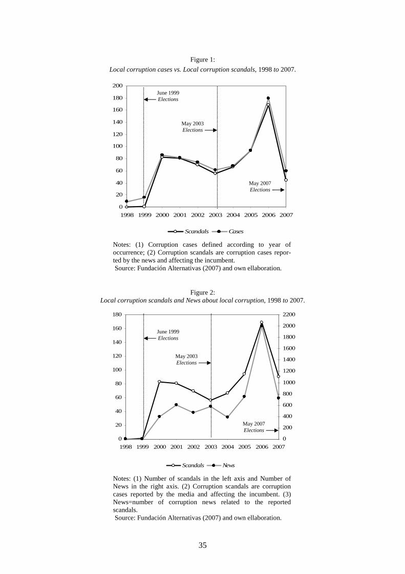
35
Figure 1:
Local corruption cases vs. Local corruption scandals, 1998 to 2007.
0
20
40
60
80
100
120
140
160
180
200
1998 1999 2000 2001 2002 2003 2004 2005 2006 2007
Scandals Cases
Notes: (1) Corruption cases defined according to year of occurrence; (2) Corruption scandals are corruption cases repor-ted by the news and affecting the incumbent. Source: Fundación Alternativas (2007) and own ellaboration.
Figure 2: Local corruption scandals and News about local corruption, 1998 to 2007.
0
20
40
60
80
100
120
140
160
180
1998 1999 2000 2001 2002 2003 2004 2005 2006 2007
0
200
400
600
800
1000
1200
1400
1600
1800
2000
2200
Scandals News
Notes: (1) Number of scandals in the left axis and Number of News in the right axis. (2) Corruption scandals are corruption cases reported by the media and affecting the incumbent. (3) News=number of corruption news related to the reported scandals. Source: Fundación Alternativas (2007) and own ellaboration.
June 1999 Elections
May 2003 Elections
May 2007 Elections
June 1999 Elections
May 2003 Elections
May 2007 Elections

36
Figure 3: News per corruption scandal and Corruption scandals, 1998 to 2007.
0
20
40
60
80
100
120
140
160
180
1998 1999 2000 2001 2002 2003 2004 2005 2006 2007
0
2
4
6
8
10
12
14
Scandals News per scandal
Notes: (1) Number of scandals in the left axis and Number of News per scandal in the right axis. (2) See Table 2. Source: Fundación Alternativas (2007) and own ellaboration.
Figure 4: % Respondents saying ‘corruption and fraud’ are among
the three worst problems of the country, Sep-2001 to Dec-2008
0.0
0.5
1.0
1.5
2.0
2.5
3.0
3.5
4.0
Sep-0
1
Feb-0
2
Jul-0
2
Dec-0
2
May-0
3
Oct-0
3
Mar-0
4
Aug-0
4
Dec-0
4
May-0
5
Oct-0
5
Mar-0
6
Aug-0
6
Jan-0
7
Jun-0
7
Nov-0
7
Apr-0
8
Sep-0
8
Source: Centro de Investigaciones Sociológicas (CIS): Baró-metro, several years.
May 2003 Elections
May 2007 Elections
June 1999 Elections
May 2003 Elections
May 2007 Elections

37
##
# # # ## #
##
##
### ##
## ##### ##
## # #### #### ##
## # ##
###
## ### ## #
## ##
# # # ## ## ###
## ##
## ### ##
##
### # ### # #### ######### #
##
#
####### #
#
##
###
# # ## # ## # ## #### ## ## ## ### # # ###
##
# # ##
##
##
# ### ###
##
#### ##### ### ### ##
# ##
#
###
### #
#
##
# ##### # # ##
##
#
#### # ## #
# ## ####
#
## ### ## # ##
#####
##
###
## ##
#
##
# #### ##### ## ##
# ## ###
##
## ### ## ## ## ##
# ##
# ### #
# ## ### ### #
## ###
#
## ### # ##
#
# ## ## ## #
### ####
# ## ###
#
#
### # #
#
###
#
## ## ## # #
###
### ### ### # ####### #
### # ##### ### # #
#
##### # ##
### ##
## ## ### # #
# #
#
##
##
#
#
##
## ## ## ##
## ##
#
##### # #
####
##
##
#
#
##
## # # #
## ## #
#### # #
## #
##
##
# ##
#
## ####
#### #
#
## ### #
#
#
## #
# ###
##
###
#
##
##
#
## #
### # ###
##
### ##
### ###
#
###
#
###
##
#
### ##
#
#
#
#
#### #
##
# # ### # ## #
##
Figure 5: % Respondents saying ‘politicians & political parties’ are among the three worst problems of the country, Jan-1995 to Dec-2008
2
4
6
8
10
12
14
16
18
20
22
Jan-9
5S
ep-9
5
May-9
6
Jan-9
7S
ep-9
7
Jun-9
8
Feb-9
9
Oct-9
9Ju
n-0
0
Feb-0
1
Nov-0
1
Jul-0
2M
ar-0
3
Nov-0
3A
ug-0
4
Apr-0
5D
ec-0
5
Aug-0
6
Apr-0
7Ja
n-0
8
Sep-0
8
Source: Centro de Investigaciones Sociológicas (CIS): Barómetro, several years.
Figure 6:
Map of corruption scandals in Spain, 1999-2007.
Source: Fundación Alternativas (2008) and own elaboration.
June 1999 Elections
May 2003 Elections
May 2007 Elections

38
Table 3:
DD estimates of the effect of Corruption scandals on incumbent’s votes. 2007 elections
(i) (ii) (iii) (iv) (v) (vi)
Corruption (dC=1 if scandal)
-0.014 (-2.13)**
-0.024 (-2.76)***
-0.030 (-3.51)***
-0.022 (-2.11)**
-0.028 (-2.75)***
-0.033 (-2.96)***
R2 0.103 0.156 0.202 0.102 0.103 0.143
F-stat. (All variables) 94.50 (0.000)
44.56 (0.000)
29.48 (0.000)
10.34 (0.000)
13.79 (0.000)
12.20 (0.000)
F-stat. (Municipal fixed effects) --.-- --.-- --.-- 28.31 (0.000)
30.33 (0.000)
25.31 (0.000)
F-stat. (Election fixed effects) 124.77 (0.000)
94.49 (0.000) --.-- 20.49
(0.000) 13.34
(0.000) --.--
F-stat. (Region × Party × Election f.e.) --.-- --.-- 35.82 (0.000) --.-- --.-- 8.22
(0.000)
F-stat. (Additional controls) --.-- 6.05
(0.000) 12.56
(0.000) --.-- 35.66
(0.000) 37.52
(0.000) Municipal fixed effects NO NO NO YES YES YES Election fixed effects YES YES NO YES YES NO Region × Party fixed effects NO NO YES NO NO YES
Additional controls NO YES YES NO YES YES
Notes: (1) Dependent variable is the increase of the incumbent party/parties vote share between 2007 and 2003 elections (∆%Vote share); (2) dC=1 if a corruption scandals affecting the incumbent was reported during the 2003-07 term; (3) Number of municipalities in the control group: 4649; Number of observations with dC=1: 294. (2) t-statistics in parenthesis; p-values in brackets; ***, ** & * = statistically significant at the 99, 95 and 90% levels. (4) Robust standard errors. (5) Additional controls include: population size dummies, property tax increase, increase in current spending, investment and debt, growth in population, housing and unemployment, and coalition dummy and party fragmentation index; see Table 1 for the definition and sources of the variables. (6) F-stat. (All variables) = test of joint statistical significance of all variables; F-stat. (Municipal fixed effects) = test of statistical significance of the municipal dummies, F-stat. (Election fixed effects) = test of statistical significance of the year dummies; F-stat. (Region × Party × Election effects) = test of statistical significance of the time × party × year dummies; F-stat. (additional controls) = test of statistical significance of the additional control variables.

39
Table 4:
DD estimates of the effect of Corruption News on incumbent’s votes. 2007 elections.
(i) (ii) (iii) (iv) (v) (vi) Corruption (dC=1 if scandal)
-0.027 (-2.32)***
-0.026 (-2.44)***
-0.026 (-2.48)***
-0.031 (-2.58)***
-0.021 (-2.61)***
-0.024 (-2.50)***
Corruption News
-0.002 (-2.34)**
--.-- --.-- --.-- -0.002 (-3.85)**
--.--
More than 5 News
--.-- -0.007 (-0.200)
--.-- --.-- --.-- --.--
More than 10 News
--.-- -0.060 (-2.33) **
-0.059 (-2.61)***
--.-- --.-- -0.097 (-2.68)***
More than 20 News
--.-- -0.001 (-0.28)
--.-- --.-- --.-- --.--
Local scandal
--.-- --.-- --.-- 0.000 (0.05)
--.-- --.--
National scandal
--.-- --.-- --.-- 0.005 (0.38)
--.-- --.--
Local news
--.-- --.-- --.-- --.-- 0.003 (2.66)***
--.--
National news
--.-- --.-- --.-- --.-- 0.001 (0.040)
--.--
More than 2 Local News
--.-- --.-- --.-- --.-- --.-- 0.044 (2.11)**
More than 5 National News
--.-- --.-- --.-- --.-- --.-- 0.015 (0.33)
R2 0.144 0.145 0.146 0.147 0.146 0.146
F-stat. (All variables) 13.80 (0.000)
9.70 (0.000)
10.03 (0.000)
17.61 (0.000)
11.57 (0.000)
10.34 (0.000)
Notes: (1) See Table 2. (2) All the estimations include: Municipal fixed effects, Region × Party fixed effects and Addi- tional controls.

40
Table 5: DD estimates of the effect of different types of Corruption scandals related to Land-use regulation on incumbent’s votes. 2007 Elections.
(i) (ii) (iii) (iv) (v) (vi) (vii) (viii) Corruption (dC=1 if scandal)
-0.031 (-2.82)**
-0.023 (-2.50)**
-0.023 (-2.70)***
-0.022 (-2.76)***
-0.019 (-1.53)
-0.020 (-1.80)*
-0.013 (-1.90)*
-0.013 (-1.71)*
Corruption News
--.-- -0.002 (-1.82)*
--.-- --.-- --.-- -0.002 (-1.28)
--.-- --.--
More than 10 News
--.-- --.-- -0.050 (-2.82)***
-0.050 (-2.99)***
--.-- --.-- -0.039 (-1.75)*
-0.040 (-1.94)*
Plan implementation
-0.001 (-0.123)
-0.002 (-0.062)
-0.001 (-0.050)
--.-- --.-- --.-- --.-- --.--
Plan enforcement
0.002 (0.61)
0.002 (0.31)
0.002 (0.18)
--.-- --.-- --.-- --.-- --.--
Public land management
-0.039 (-1.67)*
-0.039 (-1.65)*
-0.036 (-1.60)
-0.040 (-1.93)*
--.-- --.-- --.-- --.--
Environmental regulations
0.013 (0.38)
0.010 (0.34)
0.010 (0.52)
--.-- --.-- --.-- --.-- --.--
Filed
--.-- --.-- --.-- --.-- 0.045 (2.36)**
0.044 (2.52)**
0.043 (2.47)**
0.041 (2.55)**
Denounce
--.-- --.-- --.-- --.-- 0.034 (1.14)
0.034 (1.14)
0.034 (1.14)
--.--
Investigation
--.-- --.-- --.-- --.-- -0.016 (-3.77)***
-0.016 (-3.77)***
-0.016 (-3.78)***
--.--
Accusation
--.-- --.-- --.-- --.-- -0.051 (-2.09)**
-0.052 (-2.19)**
-0.050 (-2.16)**
--.--
Conviction
--.-- --.-- --.-- --.-- -0.041 (-2.88)***
-0.041 (-2.88)***
-0.041 (-2.88)***
--.--
Corruption charges
--.-- --.-- --.-- --.-- --.-- --.-- --.-- -0.054 (-2.25)**
R2 0.167 0.167 0.167 0.169 0.172 0.172 0.173 0.170 F-stat. (All variables) 28.46
(0.000) 29.59
(0.000) 29.61
(0.000) 30.10
(0.000) 61.22
(0.000) 53.25
(0.000) 54.57
(0.000) 51.33
(0.000) Notes: (1) See Table 2. . (2) All the estimations include: Municipal fixed effects, Region × Party fixed effects and Additional controls. (3) Corruption charges include only those not filed (=denounces+investigations+accusations+convictions).

41
Table 6: IV estimates of the effect of Corruption Scandals and Corruption News on incumbent’s votes. 2007 elections.
(i) (ii) (iii) (iv) (v) (vi) (vii) (viii) Corruption
-0.048 (-2.24)**
-0.047 (-2.44)**
--.-- --.-- -0.045 (-1.67)*
-0.048 (-2.11)**
-0.047 (-1.80)*
-0.048 (-1.94)*
Corruption News
--.-- --.-- -0.010 (-1.55)
-0.010 (-1.78)*
-0.004 (-1.32)
-0.006 (-1.98)**
--.-- --.--
More than 10 News
--.-- --.-- --.-- --.-- --.-- --.-- -0.128 (-1.51)
-0.122 (-1.98)**
Partial F-statistic. (1st stage) 15.61 (0.000)
13.31 (0.000)
16.67 (0.000)
15.04 (0.000)
--.-- --.-- --.-- --.--
Craig-Donald. F-statistic (1st stage) --.-- --.-- --.-- --.-- 63.31♣ 59.00♣ 49.09♣ 43.81♣
Hansen’s J over-identification St. 0.456 (0.858)
0.304 (0.834)
0.721 (0.833)
0.913 (0.859)
--.-- --.-- --.-- --.--
Region × Party fixed effects NO YES NO YES NO YES NO YES
Election fixed effects YES NO YES NO YES NO YES NO
Additional controls NO YES NO YES NO YES NO YES Notes: (1) See Table 2; (2) All estimations include Municipality fixed effects; (3) F-stat: partial F-statistic of the excluded instruments in the first-stage regression. (4) Craig-Donald F-statistic to test for weak instruments; ♣ = statistic exceeds Stock and Yogo’s weak ID tests critical values at 5% maximal IV relative bias (see Stock and Yogo, 2002); (5) Excluded instruments: beach × beach growth / vacant and urban × urban growth / vacant. (4) Hansen’s J: overidentification statistic.

42
Table 7: DD and IV estimates of the effect of Corruption Scandals and Corruption News on incumbent’s votes. 2003 elections.
DD IV (i) (ii) (iii) (iv) (v) (vi) (vii) (vii i) Corruption (dC=1 if scandal)
-0.017 (-1.99)**
--.-- -0.010 (-1.29)
-0.013 (-1.73)*
-0.032 (-1.81)*
--.-- -0.022 (-1.59)
-0.013 (-1.73)*
Corruption News
--.-- -0.001 (-2.68)***
-0.001 (-2.09)**
--.-- --.-- -0.005 (-1.71)*
-0.002 (-1.20)
--.--
More than 10 News
--.-- --.-- --.-- -0.040 (-1.27)
--.-- --.-- --.-- -0.101 (-1.537)
R2 0.244 0.234 0.231 0.229 --.-- --.-- --.-- --.--
F-stat. (All variables) 25.66 (0.000)
19.98 (0.000)
18.77 (0.000)
17.55 (0.000)
--.-- --.-- --.-- --.--
Partial F-statistic. (1st stage) --.-- --.-- --.-- --.-- 11.56 (0.000)
8.33 (0.000)
--.-- --.--
Craig-Donald. F-statistic (1st stage) --.-- --.-- --.-- --.-- --.-- --.-- 18.09 22.57♣
Hansen’s J over-identification St. --.-- --.-- --.-- --.-- 1.115 (0.534)
0.998 (0.570)
--.-- --.--
Notes: (1) See Tables 2 and 5. (2) All the estimations include: Municipal fixed effects, Region × Party fixed effects and Additional controls.

43
Table 8:
IV estimates of the effect of Corruption on votes by Ideology and Government type. 2007 elections.
(a) Ideology (b) Government type
(i) Left
(ii) Right
(iii) PSOE
(iv) PP
(v) One Party
(vi) Coalition
(vii) Mayor
(viii) Partners
Corruption
-0.060 (-1.94)*
-0.047 (-1.90)*
-0.093 (-2.19)**
-0.065 (-1.94)*
-0.048 (-1.89)*
-0.050 (-2.03)**
-0.052 (-2.35)**
0.012 (0.56)
More than 10 News
-0.163 (-2.50)**
-0.081 (-1.65)*
-0.211 (-1.93)*
-0.101 (-1.43)
-0.119 (-2.95)***
-0.138 (-2.28)**
-0.142 (-2.15)**
0.051 (0.67)
Craig-Donald. F-statistic (1st stage) 33.36♣ 41.70♣ 36.79♣ 90.95♣ 20.47♣ 27.70♣ 28.41♣ 28.23♣ Notes: (1) See Tables 2 and 5. (2) All the estimation include: Municipal fixed effects, Region × Party fixed effects and Additional controls.
Table 9: IV estimates of the effect of Corruption on votes by Voters’ traits. 2007 elections.
(a) % Construction
(b) % Unemployed
(c) % Homeowners
(d) % Commuters
(i) Low
(ii) High
(iii) Low
(iv) High
(v) Low
(vi) High
(vii) Low
(viii) High
Corruption
-0.112 (-2.65)*
-0.035 (-1.64)*
-0.052 (-2.35)**
-0.011 (-1.76)*
-0.050 (-2.11)**
-0.051 (-2.23)**
-0.052 (-1.68)*
-0.051 (-1.75)*
More than 10 News
-0.164 (-2.32)**
-0.082 (-1.56)
-0.151 (-2.06)**
-0.035 (-1.59)
-0.127 (-1.89)*
-0.116 (-1.78)*
-0.054 (-1.66)**
-0.153 (-2.68)**
Craig-Donald. F-statistic (1st stage) 30.40♣ 28.90♣ 27.70♣ 25.60♣ 26.70♣ 28.49♣ 48.43♣ 22.88♣ Notes: (1) See Tables 2 and 5. (2) All the estimation include: Municipal fixed effects, Region × Party fixed effects and Additional controls.