Embed Size (px)
Citation preview
May, 2005
Brethour, Time DomainSlide 1
doc.: IEEE 802.15-05-0246-01-004a
Submission
Project: IEEE P802.15 Working Group for Wireless Personal Area Networks (WPANs)
Submission Title: [Header Length Comments]
Date Submitted: [10 May, 2005]
Source: [Vern Brethour] Company [Time Domain Corp.]Address [7057 Old Madison Pike; Suite 250; Huntsville, Alabama 35806; USA]Voice:[(256) 428-6331], FAX: [(256) 922-0387], E-Mail: [[email protected]]
Re: [802.15.4a.]
Abstract: [Companion discussion for a corrected spreadsheet contributed as IEEE802.15-05-0245r1.]
Purpose: [To provoke a discussion of header lengths in 802.15.4a.]
Notice: This document has been prepared to assist the IEEE P802.15. It is offered as a basis for discussion and is not binding on the contributing individual(s) or organization(s). The material in this document is subject to change in form and content after further study. The contributor(s) reserve(s) the right to add, amend or withdraw material contained herein.
Release: The contributor acknowledges and accepts that this contribution becomes the property of IEEE and may be made publicly available by P802.15.
May, 2005
Brethour, Time DomainSlide 2
doc.: IEEE 802.15-05-0246-01-004a
Submission
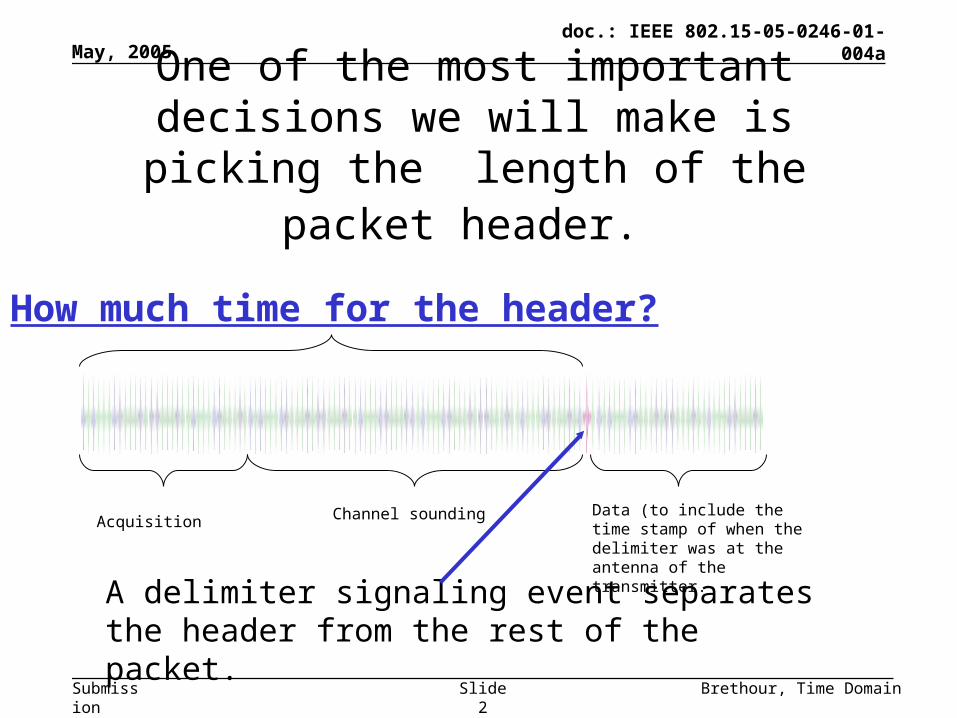
One of the most important decisions we will make is picking the length of the packet header.
Acquisition Channel sounding Data (to include the time stamp of when the delimiter was at the antenna of the transmitter.
A delimiter signaling event separates the header from the rest of the packet.
How much time for the header?
May, 2005
Brethour, Time DomainSlide 3
doc.: IEEE 802.15-05-0246-01-004a
Submission
The length of the packet header plays a huge roll in determining our long range
positioning performance.
• Our Standard is about the signal on the air.
• The Signal on the air must support our performance targets.
• Yet our performance is also largely determined by the receiver.
May, 2005
Brethour, Time DomainSlide 4
doc.: IEEE 802.15-05-0246-01-004a
Submission
Simulations are best for predicting performance
• Even simulators are costly, so we need something quick and simple to pick an initial direction.
• This is a companion document to 0245r1, which is a spreadsheet to quickly evaluate the impact of architectural trade-offs.
May, 2005
Brethour, Time DomainSlide 5
doc.: IEEE 802.15-05-0246-01-004a
Submission
The 0245r1 spreadsheet is full of assumptions about the receiver architecture.
• The receiver is NOT part of the standard.
• I would love to ignore the receiver, but: {The receiver does exist and it has performance determining properties.}
• So this discussion will include a reference receiver.

May, 2005
Brethour, Time DomainSlide 6
doc.: IEEE 802.15-05-0246-01-004a
Submission
Include a reference receiver …..okay, but first…….. disclaimers!
• This is not and will not be part of the standard.• There are lots of ways to build a radio.• There is absolutely no claim here that this
reference receiver is the best way to build a 15.4a radio.
• This is simply a structure to put the performance spreadsheet into some context.
May, 2005
Brethour, Time DomainSlide 7
doc.: IEEE 802.15-05-0246-01-004a
Submission
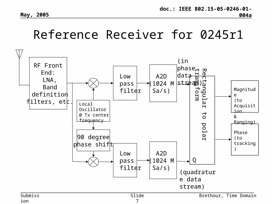
Reference Receiver for 0245r1
RF FrontEnd: LNA, Band
definition filters, etc.
A2D (1024 M
Sa/s)
Low pass filter
90 degreephase shift
Low pass filter
(in phase data stream)
(quadrature data stream)
A2D (1024 M
Sa/s)
Rectangular to polar
transform
I
Q
Magnitude(toAcquisition& Ranging)
Phase(totracking)
Local Oscillator @ Tx center frequency
May, 2005
Brethour, Time DomainSlide 8
doc.: IEEE 802.15-05-0246-01-004a
Submission
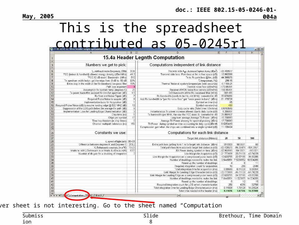
This is the spreadsheet contributed as 05-0245r1
The cover sheet is not interesting. Go to the sheet named “Computation”
May, 2005
Brethour, Time DomainSlide 9
doc.: IEEE 802.15-05-0246-01-004a
Submission
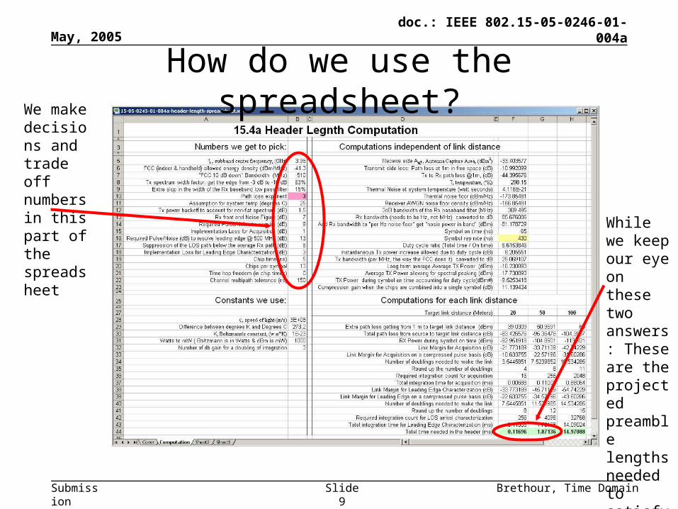
How do we use the spreadsheet?We make decisions and trade off numbers in this part of the spreadsheet
While we keep our eye on these two answers: These are the projected preamble lengths needed to satisfy the conditions
May, 2005
Brethour, Time DomainSlide 10
doc.: IEEE 802.15-05-0246-01-004a
Submission
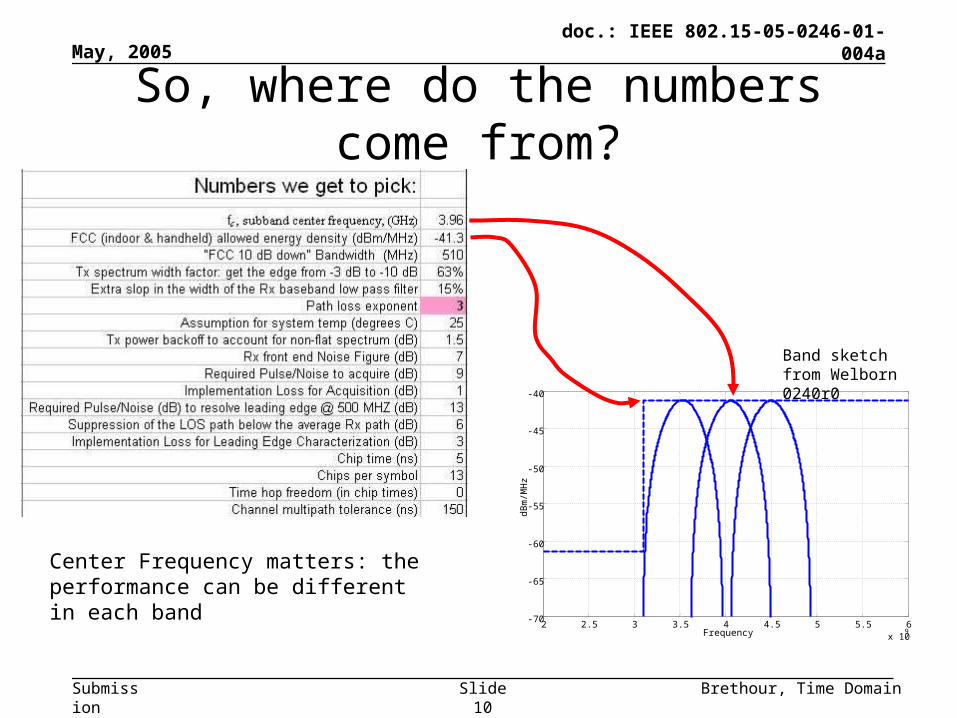
So, where do the numbers come from?
2 2.5 3 3.5 4 4.5 5 5.5 6x 10
9
-70
-65
-60
-55
-50
-45
-40
Frequency
dBm
/MH
z
Band sketch from Welborn 0240r0
Center Frequency matters: the performance can be different in each band

May, 2005
Brethour, Time DomainSlide 11
doc.: IEEE 802.15-05-0246-01-004a
Submission
More numbers
2 2.5 3 3.5 4 4.5 5 5.5 6x 10
9
-70
-65
-60
-55
-50
-45
-40
Frequency
dBm
/MH
z
Band sketch from Welborn 0240r0
Depending on how much pulse shaping we do, the 3dB Tx bandwidth might only be 63% of the 10 dB bandwidth. We must convert, because most of the calculations are with respect to a 3 dB bandwidth.
May, 2005
Brethour, Time DomainSlide 12
doc.: IEEE 802.15-05-0246-01-004a
Submission
More numbers
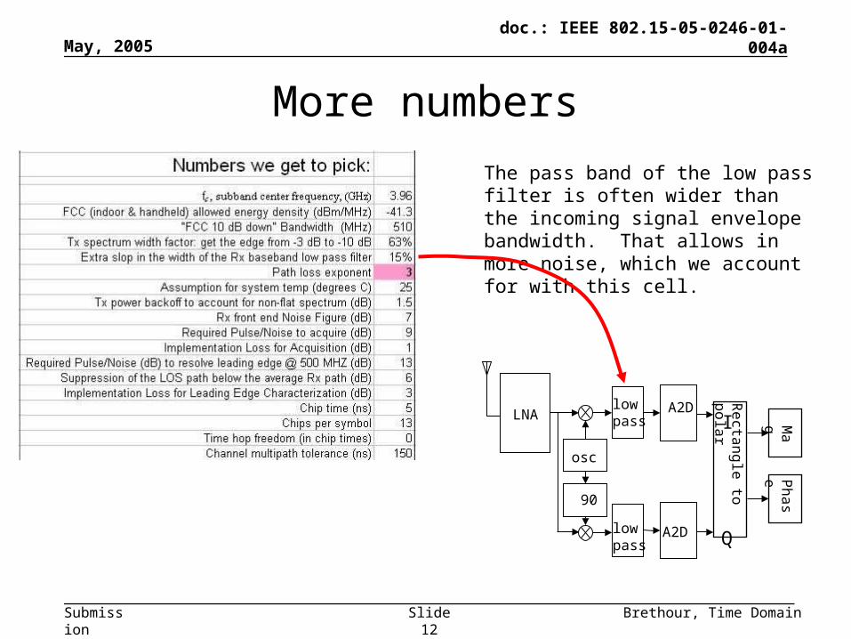
The pass band of the low pass filter is often wider than the incoming signal envelope bandwidth. That allows in more noise, which we account for with this cell.
I
Q
osc
90
lowpass
lowpassLNA A2D
A2D
Rectangle to
polar
Pha
seMag
May, 2005
Brethour, Time DomainSlide 13
doc.: IEEE 802.15-05-0246-01-004a
Submission
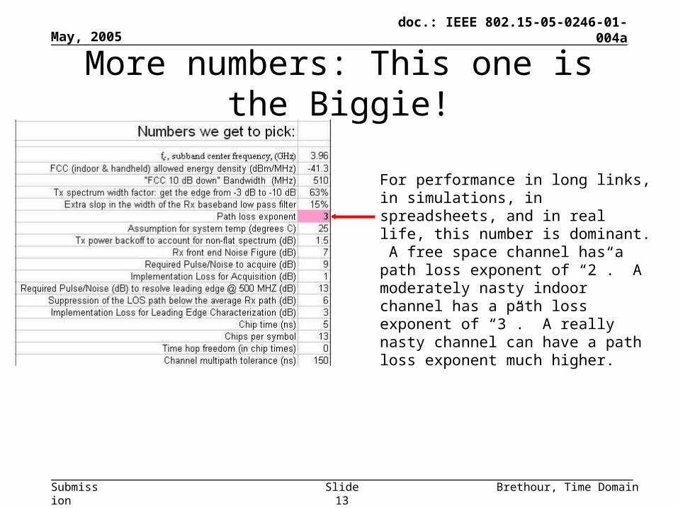
More numbers: This one is the Biggie!
For performance in long links, in simulations, in spreadsheets, and in real life, this number is dominant. A free space channel has a path loss exponent of “2”. A moderately nasty indoor channel has a path loss exponent of “3”. A really nasty channel can have a path loss exponent much higher.
May, 2005
Brethour, Time DomainSlide 14
doc.: IEEE 802.15-05-0246-01-004a
Submission
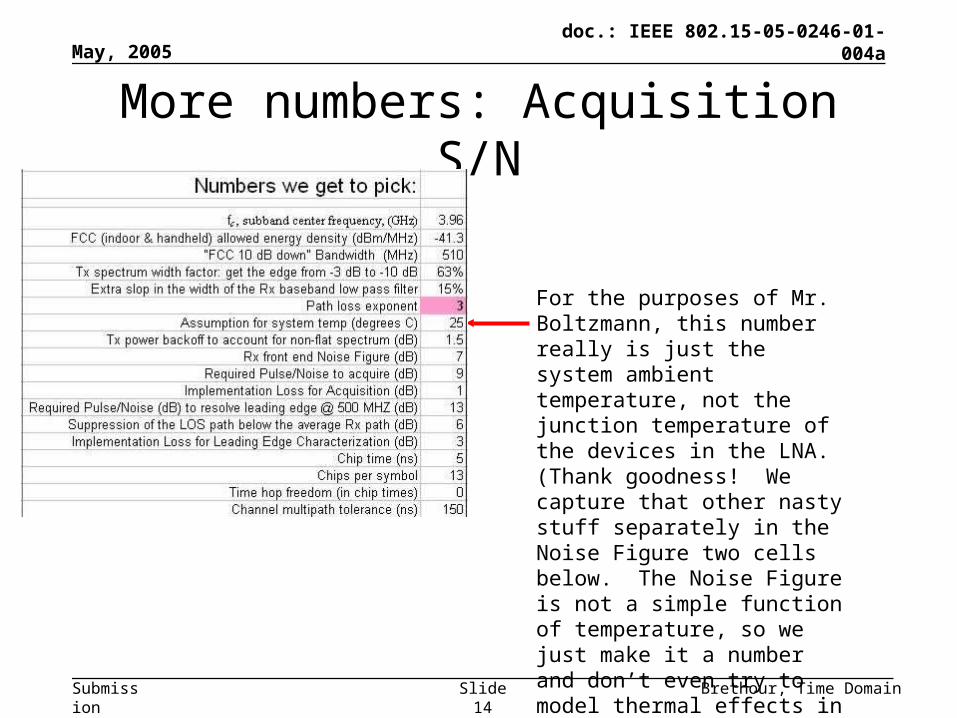
More numbers: Acquisition S/N
For the purposes of Mr. Boltzmann, this number really is just the system ambient temperature, not the junction temperature of the devices in the LNA. (Thank goodness! We capture that other nasty stuff separately in the Noise Figure two cells below. The Noise Figure is not a simple function of temperature, so we just make it a number and don’t even try to model thermal effects in the NF.)

May, 2005
Brethour, Time DomainSlide 15
doc.: IEEE 802.15-05-0246-01-004a
Submission
More numbers :
2 2.5 3 3.5 4 4.5 5 5.5 6x 10
9
-70
-65
-60
-55
-50
-45
-40
Frequency
dBm
/MH
z
Band sketch from Welborn 0240r0
By the time we get done building the Tx and take it to the compliance test lab, the output spectrum will never be as smooth as the blue curves. We must then back off the Tx power across the entire band to keep the worst little spike below the FCC emissions mask.

May, 2005
Brethour, Time DomainSlide 16
doc.: IEEE 802.15-05-0246-01-004a
Submission
More numbers
A 7dB noise figure will sound high to people used to narrow band radios.
This is UWB , and we’re targeting a system we can build in CMOS
I
Q
osc
90
lowpass
lowpassLNA A2D
A2D
Rectangle to
polar
Pha
seMag

May, 2005
Brethour, Time DomainSlide 17
doc.: IEEE 802.15-05-0246-01-004a
Submission
More numbers: Acquisition S/N
This number is an estimate of the post-integration S/N needed to acquire with a high probability of detect as well as a low probability of false alarm. Even after extensive simulations, it is often hard to get consensus on this number. It’s certainly more than 6 dB. 9 dB is a reasonable guess. Others are free to make their own guesses.
May, 2005
Brethour, Time DomainSlide 18
doc.: IEEE 802.15-05-0246-01-004a
Submission
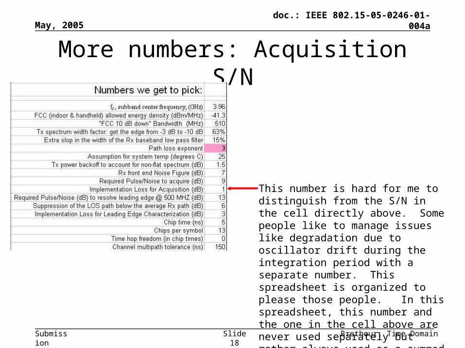
More numbers: Acquisition S/N
This number is hard for me to distinguish from the S/N in the cell directly above. Some people like to manage issues like degradation due to oscillator drift during the integration period with a separate number. This spreadsheet is organized to please those people. In this spreadsheet, this number and the one in the cell above are never used separately but rather always used as a summed pair.
May, 2005
Brethour, Time DomainSlide 19
doc.: IEEE 802.15-05-0246-01-004a
Submission
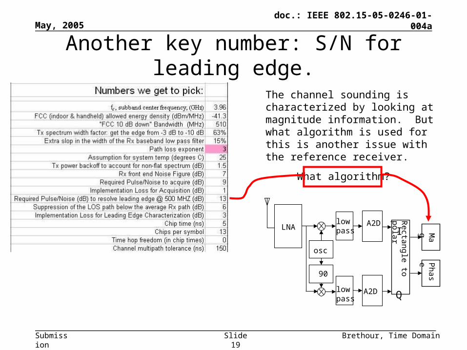
Another key number: S/N for leading edge.
The channel sounding is characterized by looking at magnitude information. But what algorithm is used for this is another issue with the reference receiver.
I
Q
osc
90
lowpass
lowpassLNA A2D
A2D
Rectangle to
polar
Pha
seMag
What algorithm?
May, 2005
Brethour, Time DomainSlide 20
doc.: IEEE 802.15-05-0246-01-004a
Submission
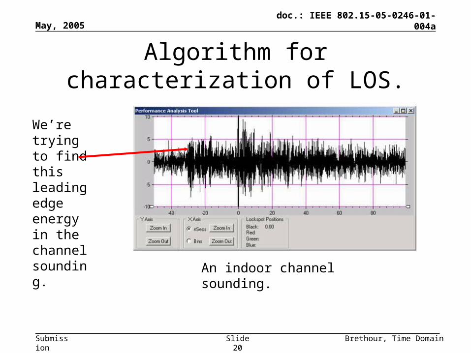
Algorithm for characterization of LOS.
An indoor channel sounding.
We’re trying to find this leading edge energy in the channel sounding.
May, 2005
Brethour, Time DomainSlide 21
doc.: IEEE 802.15-05-0246-01-004a
Submission
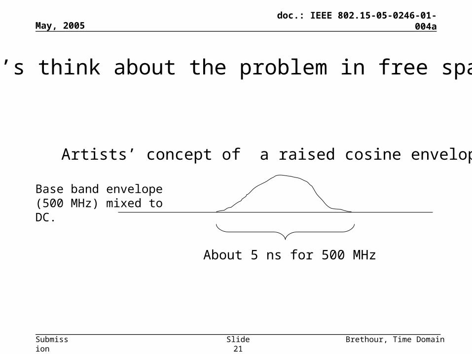
Base band envelope (500 MHz) mixed to DC.
Artists’ concept of a raised cosine envelope
About 5 ns for 500 MHz
Let’s think about the problem in free space:
May, 2005
Brethour, Time DomainSlide 22
doc.: IEEE 802.15-05-0246-01-004a
Submission
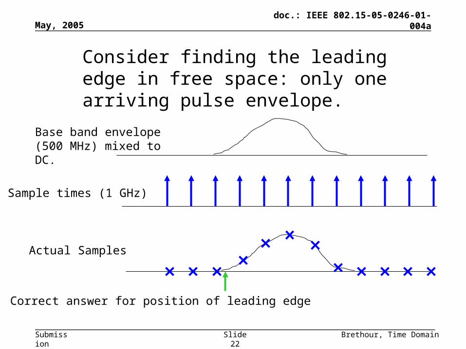
Base band envelope (500 MHz) mixed to DC.
Sample times (1 GHz)
Actual Samples
Correct answer for position of leading edge
Consider finding the leading edge in free space: only one arriving pulse envelope.
May, 2005
Brethour, Time DomainSlide 23
doc.: IEEE 802.15-05-0246-01-004a
Submission
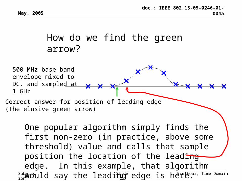
500 MHz base band envelope mixed to DC. and sampled at 1 GHz
Correct answer for position of leading edge (The elusive green arrow)
How do we find the green arrow?
One popular algorithm simply finds the first non-zero (in practice, above some threshold) value and calls that sample position the location of the leading edge. In this example, that algorithm would say the leading edge is here.
May, 2005
Brethour, Time DomainSlide 24
doc.: IEEE 802.15-05-0246-01-004a
Submission
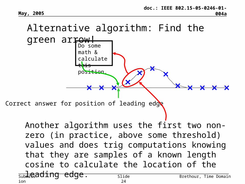
Correct answer for position of leading edge
Alternative algorithm: Find the green arrow!
Another algorithm uses the first two non-zero (in practice, above some threshold) values and does trig computations knowing that they are samples of a known length cosine to calculate the location of the leading edge.
Do some math & calculate this position.
May, 2005
Brethour, Time DomainSlide 25
doc.: IEEE 802.15-05-0246-01-004a
Submission
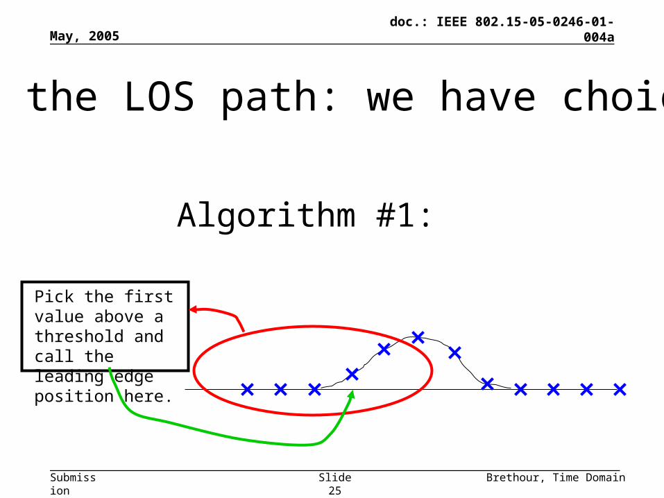
Pick the first value above a threshold and call the leading edge position here.
Find the LOS path: we have choices!
Algorithm #1:

May, 2005
Brethour, Time DomainSlide 26
doc.: IEEE 802.15-05-0246-01-004a
Submission
Find the LOS path: we have choices!
Algorithm #2:
Do some math & calculate this position.
May, 2005
Brethour, Time DomainSlide 27
doc.: IEEE 802.15-05-0246-01-004a
Submission
Trig. look up table
Pick 1st big one
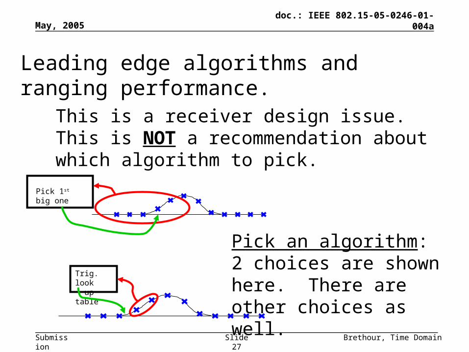
Pick an algorithm: 2 choices are shown here. There are other choices as well.
This is a receiver design issue. This is NOT a recommendation about which algorithm to pick.
Leading edge algorithms and ranging performance.

May, 2005
Brethour, Time DomainSlide 28
doc.: IEEE 802.15-05-0246-01-004a
Submission
Algorithm selection determines the S/N value.
The modeling of this algorithm is where this particular number comes from.
trigonometry
May, 2005
Brethour, Time DomainSlide 29
doc.: IEEE 802.15-05-0246-01-004a
Submission
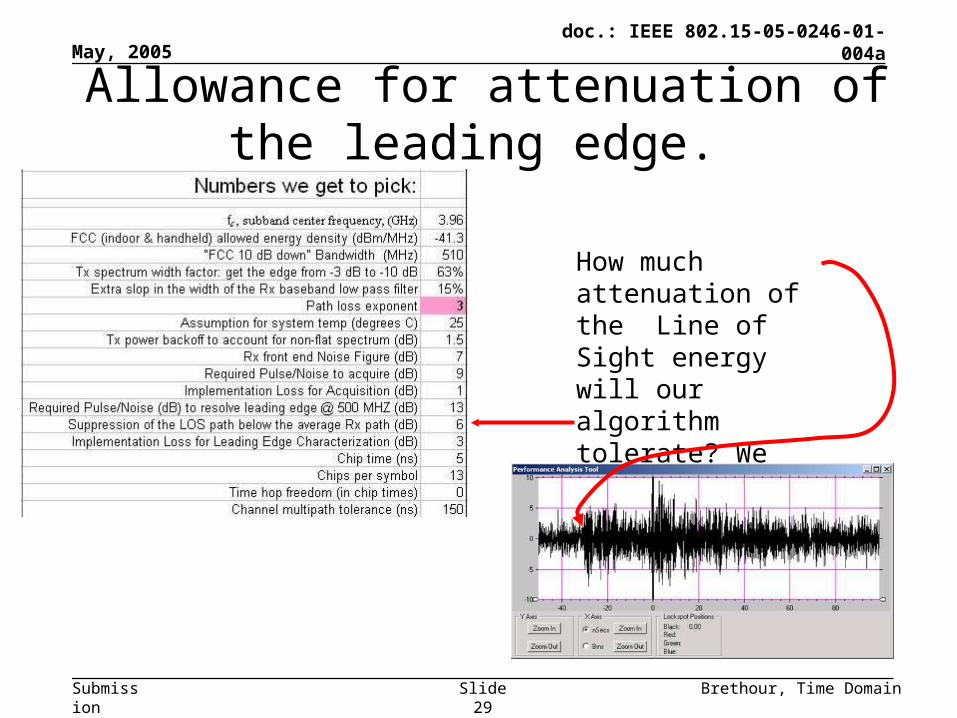
Allowance for attenuation of the leading edge.
How much attenuation of the Line of Sight energy will our algorithm tolerate? We make allowance for that here.

May, 2005
Brethour, Time DomainSlide 30
doc.: IEEE 802.15-05-0246-01-004a
Submission
LOS algorithm implementation loss.
This number captures stray effects like imperfect tracking of oscillator drift during the channel sounding and round-off errors in trig tables and such distractions. I find it useful to characterize the S/N needed for the algorithm (two cells above) as if everything about the implementation of the algorithm were perfect and then account for imperfections separately here.
May, 2005
Brethour, Time DomainSlide 31
doc.: IEEE 802.15-05-0246-01-004a
Submission
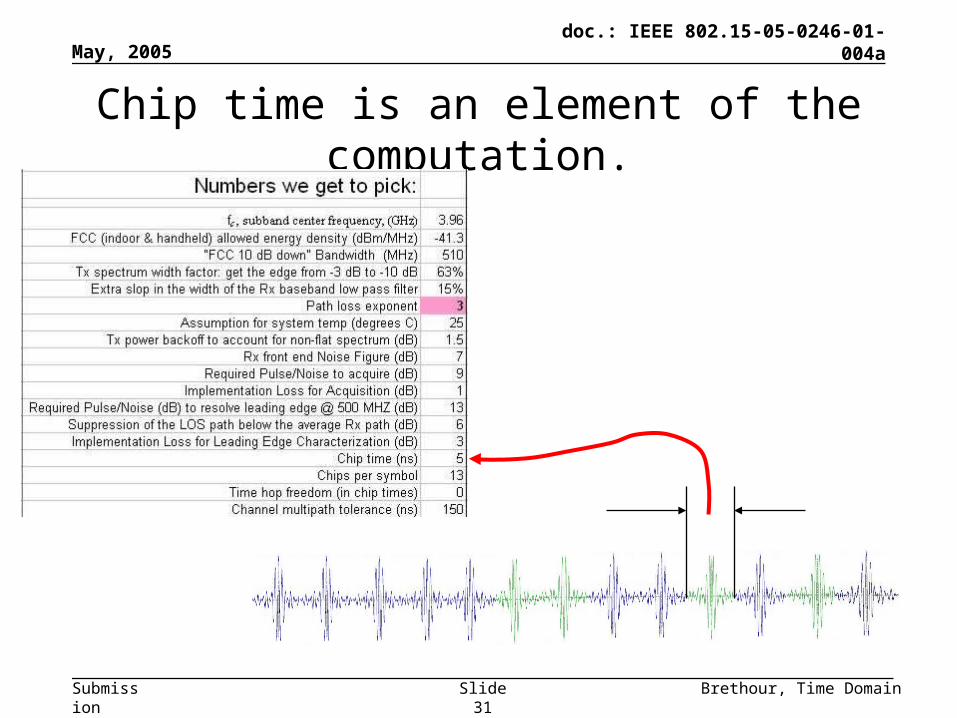
Chip time is an element of the computation.
May, 2005
Brethour, Time DomainSlide 32
doc.: IEEE 802.15-05-0246-01-004a
Submission
1 2 3 4 5 6 7 8 9 10 11 12 13
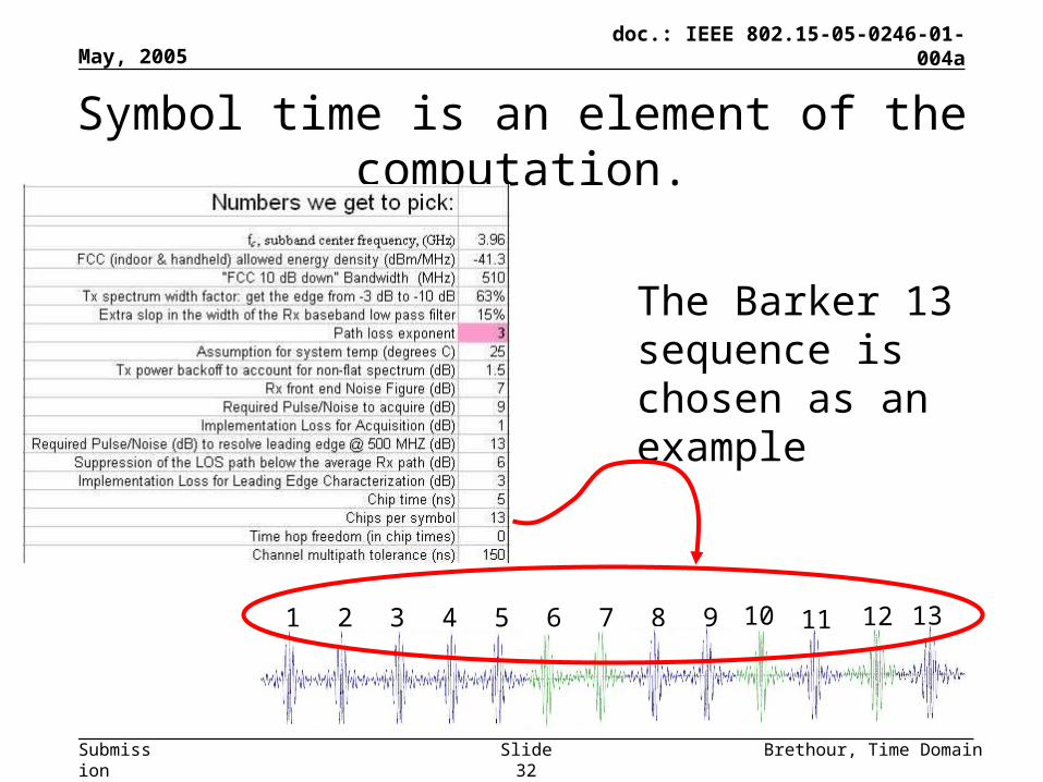
The Barker 13 sequence is chosen as an example
Symbol time is an element of the computation.
May, 2005
Brethour, Time DomainSlide 33
doc.: IEEE 802.15-05-0246-01-004a
Submission
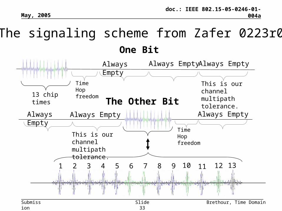
13 chip times
One Bit
The Other Bit
Time Hopfreedom
Always EmptyAlways Empty
Always EmptyAlways Empty Always Empty
Always Empty
The signaling scheme from Zafer 0223r0
Time Hopfreedom
This is our channel multipath tolerance.
This is our channel multipath tolerance.
1 2 3 4 5 6 7 8 9 10 11 12 13
May, 2005
Brethour, Time DomainSlide 34
doc.: IEEE 802.15-05-0246-01-004a
Submission
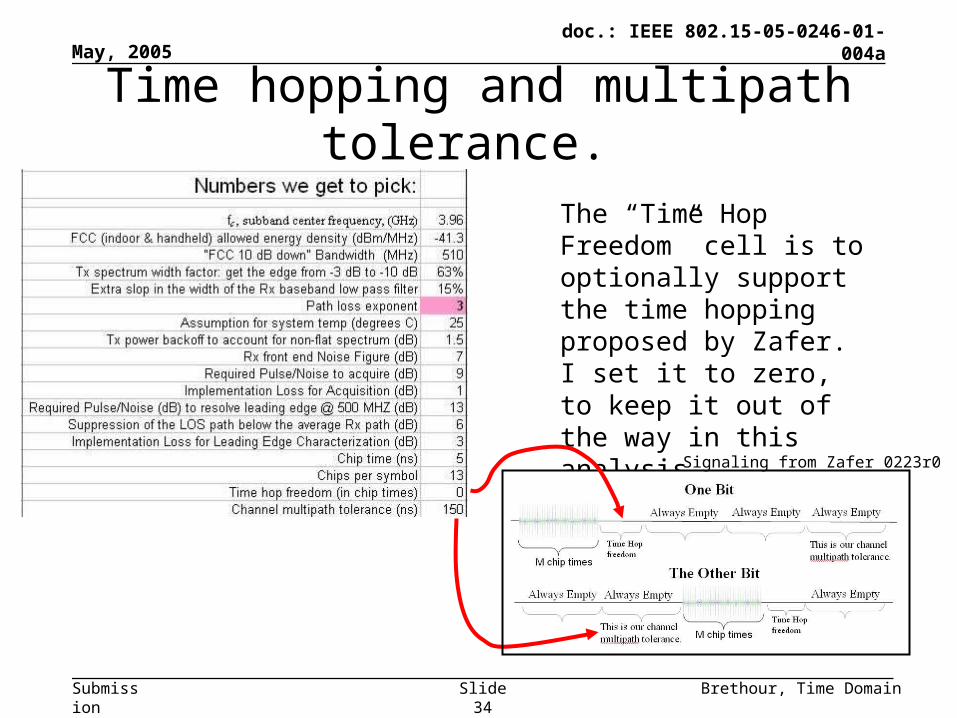
The “Time Hop Freedom” cell is to optionally support the time hopping proposed by Zafer. I set it to zero, to keep it out of the way in this analysis.
Time hopping and multipath tolerance.
Signaling from Zafer 0223r0
May, 2005
Brethour, Time DomainSlide 35
doc.: IEEE 802.15-05-0246-01-004a
Submission
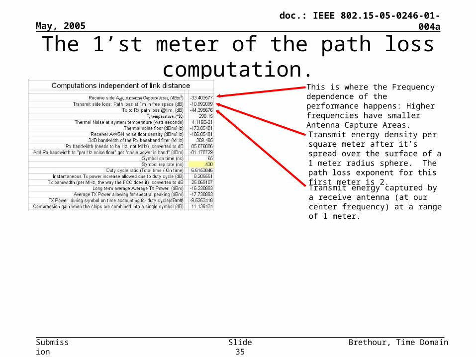
The 1’st meter of the path loss computation.This is where the Frequency dependence of the performance happens: Higher frequencies have smaller Antenna Capture Areas.
Transmit energy density per square meter after it’s spread over the surface of a 1 meter radius sphere. The path loss exponent for this first meter is 2.
Transmit energy captured by a receive antenna (at our center frequency) at a range of 1 meter.
May, 2005
Brethour, Time DomainSlide 36
doc.: IEEE 802.15-05-0246-01-004a
Submission
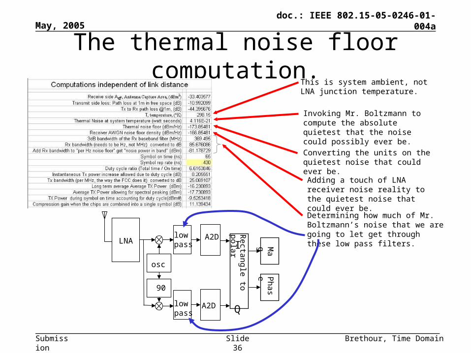
The thermal noise floor computation.This is system ambient, not LNA junction temperature.
Invoking Mr. Boltzmann to compute the absolute quietest that the noise could possibly ever be.
Converting the units on the quietest noise that could ever be.
Adding a touch of LNA receiver noise reality to the quietest noise that could ever be.
Determining how much of Mr. Boltzmann’s noise that we are going to let get through these low pass filters.
I
Q
osc
90
lowpass
lowpassLNA A2D
A2D
Rectangle to
polar
Pha
seMag
May, 2005
Brethour, Time DomainSlide 37
doc.: IEEE 802.15-05-0246-01-004a
Submission
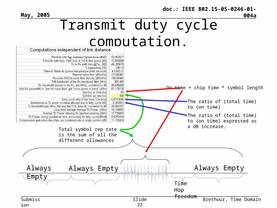
Transmit duty cycle computation.
Always EmptyAlways Empty Always Empty
Time Hopfreedom
On time = chip time * symbol length
Total symbol rep rate is the sum of all the different allowances
The ratio of {total time} to {on time}
The ratio of {total time} to {on time} expressed as a dB increase.
May, 2005
Brethour, Time DomainSlide 38
doc.: IEEE 802.15-05-0246-01-004a
Submission
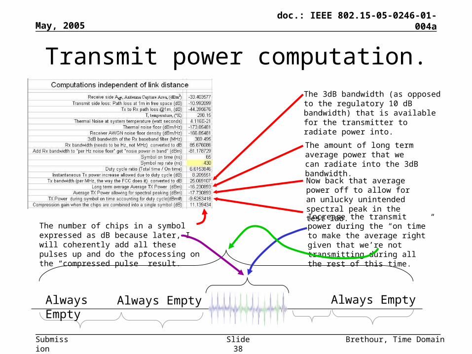
Transmit power computation.
Always EmptyAlways Empty Always Empty
The 3dB bandwidth (as opposed to the regulatory 10 dB bandwidth) that is available for the transmitter to radiate power into.
The amount of long term average power that we can radiate into the 3dB bandwidth.
Now back that average power off to allow for an unlucky unintended spectral peak in the test lab.
Increase the transmit power during the “on time” to make the average right given that we’re not transmitting during all the rest of this time.
The number of chips in a symbol expressed as dB because later, I will coherently add all these pulses up and do the processing on the “compressed pulse” result.

May, 2005
Brethour, Time DomainSlide 39
doc.: IEEE 802.15-05-0246-01-004a
Submission
The path loss computations for each target.
The target distance in meters that we’re going to evaluate. This number is user changeable if we want to try another distance. There is an assumption that the distance will be long. If it is short, the assumptions about the signs of the numbers breaks down and the answers are garbage.
Path loss calculated using the deadly Path Loss Exponent.
Total path loss which now includes the first meter, the rest of the meters, as well as the capture area of the receive antenna.
Rx power is the Tx power plus the path loss.
May, 2005
Brethour, Time DomainSlide 40
doc.: IEEE 802.15-05-0246-01-004a
Submission
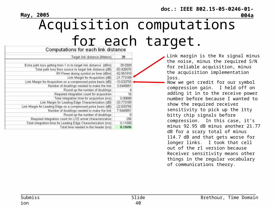
Acquisition computations for each target.
Link margin is the Rx signal minus the noise, minus the required S/N for reliable acquisition, minus the acquisition implementation loss.
Now we get credit for our symbol compression gain. I held off on adding it in to the receive power number before because I wanted to show the required receiver sensitivity to pick up the itty bitty chip signals before compression. In this case, it’s minus 92.95 dB minus another 21.77 dB for a scary total of minus 114.7 dB and that gets worse for longer links. I took that cell out of the r1 version because Receiver sensitivity means other things in the regular vocabulary of communications theory.

May, 2005
Brethour, Time DomainSlide 41
doc.: IEEE 802.15-05-0246-01-004a
Submission
Acquisition header computations.
The negative link margin tells how much gain is needed to successfully do the job. I get this gain by doubling by integration as often as required. Dividing the link margin by 3 dB per integration doubling, yields how many doublings are required.
To keep the implementation easy, we only want to have integration counts which are powers of 2. So here we round the number of doublings up to the next biggest integer.
2 raised to the number of doublings gives the needed integration count
The integration count times the symbol repetition period equals the number of ms of header time needed for acquisition.
May, 2005
Brethour, Time DomainSlide 42
doc.: IEEE 802.15-05-0246-01-004a
Submission
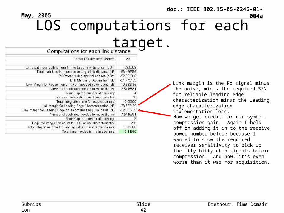
LOS computations for each target.
Link margin is the Rx signal minus the noise, minus the required S/N for reliable leading edge characterization minus the leading edge characterization implementation loss.
Now we get credit for our symbol compression gain. Again I held off on adding it in to the receive power number before because I wanted to show the required receiver sensitivity to pick up the itty bitty chip signals before compression. And now, it’s even worse than it was for acquisition.
May, 2005
Brethour, Time DomainSlide 43
doc.: IEEE 802.15-05-0246-01-004a
Submission
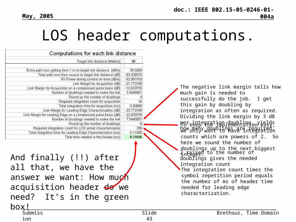
LOS header computations.
The negative link margin tells how much gain is needed to successfully do the job. I get this gain by doubling by integration as often as required. Dividing the link margin by 3 dB per integration doubling, yields how many doublings are required.
To keep the implementation easy, we only want to have integration counts which are powers of 2. So here we round the number of doublings up to the next biggest integer.
2 raised to the number of doublings gives the needed integration count
The integration count times the symbol repetition period equals the number of ms of header time needed for leading edge characterization.
And finally (!!) after all that, we have the answer we want: How much acquisition header do we need? It’s in the green box!
May, 2005
Brethour, Time DomainSlide 44
doc.: IEEE 802.15-05-0246-01-004a
Submission
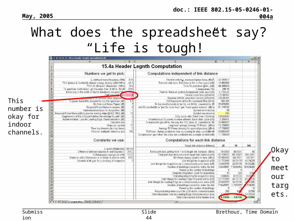
What does the spreadsheet say?“Life is tough!”
This number is okay for indoor channels.
Okay to meet our targets.
May, 2005
Brethour, Time DomainSlide 45
doc.: IEEE 802.15-05-0246-01-004a
Submission
Conclusion: We should stick with our ranging performance targets, for now.
• 50 meter positioning to 1 meter accuracy in under 10 ms (per round trip, with a small allowance for overhead) looks doable.
• 20 meter positioning to 1 meter accuracy in under 2 ms (per round trip, with a small allowance for overhead) also looks doable.
• These performance targets are only hard, not impossible.
• There are other positioning solutions in the marketplace, but if we hit these targets (or get close) we will bring unique value to our customers.

![IEEE Life Cycle Standards and the CMMI Implementation Considerations · 2017-05-19 · [IEEE 1998] IEEE 1062, IEEE Recommended Practice for Software Acquisition [IEEE 2005] IEEE 15288,](https://img.pdfslide.net/doc/110x75/5e740ab442e6042c3d2f498e/ieee-life-cycle-standards-and-the-cmmi-implementation-considerations-2017-05-19.jpg)