POLITECNICO DI MILANOCorso di Laurea Magistrale in Ingegneria Informatica

Dipartimento di Elettronica, Informazione e BioingegneriaScuola di Ingegneria Industriale e dell’Informazione

DockerCap:A software-level power capping orchestrator

for Docker containers

NECSTLabNovel, Emerging Computing System Technologies Laboratory

presso il Politecnico di Milano

Relatore: Prof. Marco Domenico SANTAMBROGIOCorrelatore: Dott. Matteo FERRONI

Tesi di Laurea di:Amedeo ASNAGHI, matricola 816939

Anno Accademico 2015-2016

Alla mia famiglia e a Valentina

AA

Contents

Abstract VIII

Sommario IX

Ringraziamenti XIII

1 Introduction 1

2 State of the art 62.1 Power capping . . . . . . . . . . . . . . . . . . . . . . . . . . . . . . . . . 62.2 Virtualization and Containerization . . . . . . . . . . . . . . . . . . . . . . 92.3 Fog Computing . . . . . . . . . . . . . . . . . . . . . . . . . . . . . . . . . 102.4 Control Theory . . . . . . . . . . . . . . . . . . . . . . . . . . . . . . . . . 11

3 Problem definition 123.1 Preliminary definitions . . . . . . . . . . . . . . . . . . . . . . . . . . . . . 123.2 Problem statement . . . . . . . . . . . . . . . . . . . . . . . . . . . . . . . 13

4 Proposed methodology 174.1 DockerCap in a nutshell . . . . . . . . . . . . . . . . . . . . . . . . . . . . 174.2 Observe Phase . . . . . . . . . . . . . . . . . . . . . . . . . . . . . . . . . 194.3 Decide Phase . . . . . . . . . . . . . . . . . . . . . . . . . . . . . . . . . . 21

4.3.1 Resource Control . . . . . . . . . . . . . . . . . . . . . . . . . . . . 234.3.2 Resource Partitioning . . . . . . . . . . . . . . . . . . . . . . . . . 26

4.4 Act Phase . . . . . . . . . . . . . . . . . . . . . . . . . . . . . . . . . . . . 32

5 Implementation 345.1 Implementation goals . . . . . . . . . . . . . . . . . . . . . . . . . . . . . . 345.2 Proposed system architecture . . . . . . . . . . . . . . . . . . . . . . . . . 35

5.2.1 Observe Component . . . . . . . . . . . . . . . . . . . . . . . . . . 365.2.2 Decide Component . . . . . . . . . . . . . . . . . . . . . . . . . . . 385.2.3 Act Component . . . . . . . . . . . . . . . . . . . . . . . . . . . . . 44

6 Experimental results 466.1 Experimental Setup . . . . . . . . . . . . . . . . . . . . . . . . . . . . . . 466.2 Precision Evaluation . . . . . . . . . . . . . . . . . . . . . . . . . . . . . . 48

I

6.3 Performance Evaluation . . . . . . . . . . . . . . . . . . . . . . . . . . . . 51

7 Conclusions and Future work 55

Bibliography 58

A DockerCap configuration A.1

List of Figures

1.1 The Internet of Things and Fog Computing architecture [1] . . . . . . . . 2

2.1 Virtualization and Containerization schema . . . . . . . . . . . . . . . . . 10

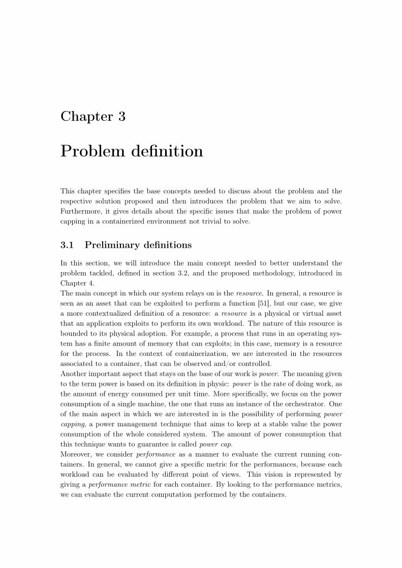
3.1 Relationship between power consumption and CPU quota. In the providedexample, we perform multiple runs of fluidanimate from the PARSECbenchmark suite [52] in a Docker container and we vary the CPU Quotaassociated to it across the different runs . . . . . . . . . . . . . . . . . . . 14

3.2 Relationship between Time to completion (TTC) and CPU quota (loweris better) We perform multiple runs of fluidanimate from the PARSECbenchmark suite, considering as performance metric the TTC of the bench-mark, with different allocation of CPU quota . . . . . . . . . . . . . . . . 14

3.3 Dependence with respect to the type of workload. This shows how thepower consumption is strongly dependent from the type of workload. Weperform two distinct runs of two different benchmark, fluidanimate anddedup from the PARSEC benchmark suite [52] and we show how the powerconsumption of the same machine differs from one run to the other. . . . . 15

3.4 Dependence with respect to the allocation of the containers. We performtwo distinct runs of two distinct allocation of container, one with fluidan-imate and dedup and the other with fluidanimate and x264, all from thePARSEC benchmark suit. Even if we change only one workload from therunning containers, the power consumption changes significantly. . . . . . 16

4.1 General structure of DockerCap . . . . . . . . . . . . . . . . . . . . . . . . 184.2 General structure of the Observe Phase . . . . . . . . . . . . . . . . . . . 194.3 Power sample sampled overtime during an Observation . . . . . . . . . . . 204.4 General structure of the Decide Phase . . . . . . . . . . . . . . . . . . . . 224.5 Inputs and output of the Resource Control subphase . . . . . . . . . . . . 234.6 Feedback control loop exploited in the Resource Control phase . . . . . . . 244.7 Inputs and output of the Resource Partitioning subphase . . . . . . . . . . 274.8 Graphical representation of the Fair resource partitioning . . . . . . . . . 284.9 Graphical representation of the Priority-aware resource partitioning . . . . 294.10 Graphical representation of the Throughput-aware resource partitioning . 30

III

4.11 Relationship between the CPU quota and the resource assigned to the con-tainer. It can be seen that all the considered workloads from the PARSECbenchmark suite follow a hyperbola . . . . . . . . . . . . . . . . . . . . . . 31

4.12 General structure of the Act Phase . . . . . . . . . . . . . . . . . . . . . . 33

5.1 Runtime architecture of DockerCap . . . . . . . . . . . . . . . . . . . . . . 355.2 Class diagram of the Controller and Partitioner interfaces with the re-

spective implemented policies . . . . . . . . . . . . . . . . . . . . . . . . . 45

6.1 Power consumption of the server under different power caps, controlled bythe ARX Fair partitioning policy and the Linear Fair partitioning policyin different value of p. The results obtained with RAPL are reported asreference . . . . . . . . . . . . . . . . . . . . . . . . . . . . . . . . . . . . . 49

6.2 Power consumption of the server under different power caps, controlled bythe three proposed Partitioning policy with the ARX model used in thecontroller . . . . . . . . . . . . . . . . . . . . . . . . . . . . . . . . . . . . 50

6.3 Performance comparison between the Fair resource partitioning policy andRAPL with respect to three different power caps. (lower is better) . . . . 52

6.4 Performance comparison between the Fair resource partitioning policy, thePriority-aware partitioning policy and the Throughput-aware partitioningpolicy, with respect to three different power caps (lower is better). . . . . 53

List of Algorithms

1 Observe Component pseudocode . . . . . . . . . . . . . . . . . . . . . . . 372 Decide Component pseudocode . . . . . . . . . . . . . . . . . . . . . . . . 393 Decider pseudocode . . . . . . . . . . . . . . . . . . . . . . . . . . . . . . . 394 ARX resource control policy . . . . . . . . . . . . . . . . . . . . . . . . . . 405 Linear resource control policy . . . . . . . . . . . . . . . . . . . . . . . . . 416 Fair resource partitioning . . . . . . . . . . . . . . . . . . . . . . . . . . . 417 Priority-aware resource partitioning . . . . . . . . . . . . . . . . . . . . . . 428 Throughput-aware resource partitioning . . . . . . . . . . . . . . . . . . . 439 Act Component pseudocode . . . . . . . . . . . . . . . . . . . . . . . . . . 44

List of Tables

5.1 Information gathered by the Observe Component . . . . . . . . . . . . . . 38

6.1 Experimental setup . . . . . . . . . . . . . . . . . . . . . . . . . . . . . . . 476.2 Weights of the priorities . . . . . . . . . . . . . . . . . . . . . . . . . . . . 516.3 Benchmark configurations, priorities and SLO . . . . . . . . . . . . . . . . 51

List of Listings

5.1 An example of a JSON produced by the Observe Component . . . . . . . 385.2 An example of a JSON produced by the Decide Component . . . . . . . . 44A.1 XML Configuration file of the Observe Phase . . . . . . . . . . . . . . . . A.2A.2 XML Configuration file of the Observe Phase . . . . . . . . . . . . . . . . A.3

Abstract

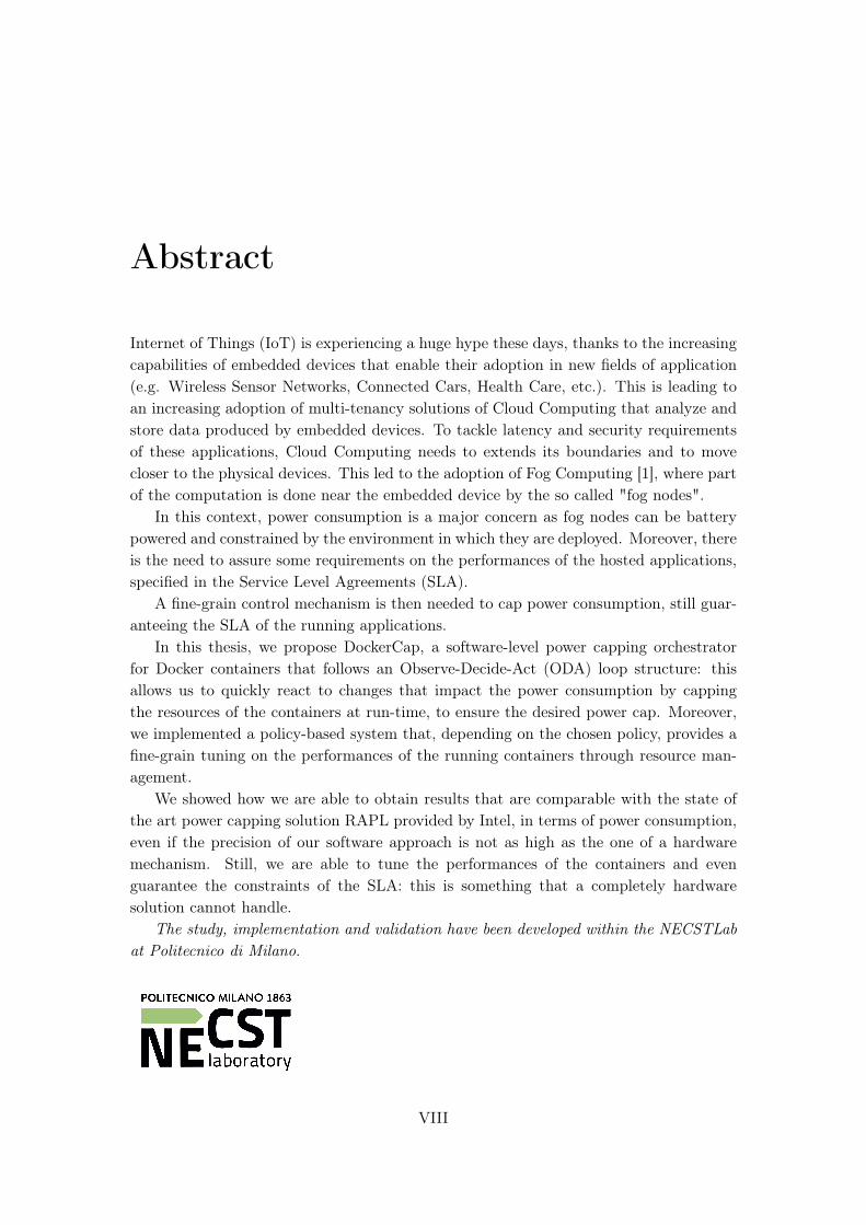
Internet of Things (IoT) is experiencing a huge hype these days, thanks to the increasingcapabilities of embedded devices that enable their adoption in new fields of application(e.g. Wireless Sensor Networks, Connected Cars, Health Care, etc.). This is leading toan increasing adoption of multi-tenancy solutions of Cloud Computing that analyze andstore data produced by embedded devices. To tackle latency and security requirementsof these applications, Cloud Computing needs to extends its boundaries and to movecloser to the physical devices. This led to the adoption of Fog Computing [1], where partof the computation is done near the embedded device by the so called "fog nodes".

In this context, power consumption is a major concern as fog nodes can be batterypowered and constrained by the environment in which they are deployed. Moreover, thereis the need to assure some requirements on the performances of the hosted applications,specified in the Service Level Agreements (SLA).

A fine-grain control mechanism is then needed to cap power consumption, still guar-anteeing the SLA of the running applications.

In this thesis, we propose DockerCap, a software-level power capping orchestratorfor Docker containers that follows an Observe-Decide-Act (ODA) loop structure: thisallows us to quickly react to changes that impact the power consumption by cappingthe resources of the containers at run-time, to ensure the desired power cap. Moreover,we implemented a policy-based system that, depending on the chosen policy, provides afine-grain tuning on the performances of the running containers through resource man-agement.

We showed how we are able to obtain results that are comparable with the state ofthe art power capping solution RAPL provided by Intel, in terms of power consumption,even if the precision of our software approach is not as high as the one of a hardwaremechanism. Still, we are able to tune the performances of the containers and evenguarantee the constraints of the SLA: this is something that a completely hardwaresolution cannot handle.

The study, implementation and validation have been developed within the NECSTLabat Politecnico di Milano.

VIII

Sommario

Negli ultimi anni, un gran numero di dispositivi viene continuamente connesso a Inter-net, introducendo il concetto di Internet of Things (IoT). L’IoT permette ai dispositivifisici di scambiare informazioni attraverso la rete, per l’acquisizione e lo scambio di dati.Oltretutto, questi dispositivi non si limitano ad osservare l’ambiente, ma possono intera-gire con esso tramite attuatori che, insieme alla rete e al software, permettono ai sistemiinformatici di interagire col mondo fisico.

La diffusione di dispositivi IoT ha portato alla produzione di una grande quantitàdi dati, che deve essere processata e memorizzata, ma i singoli dispositivi non sonoin grado dare queste funzionalità, per limiti in capacità computazionali e energetici.Questo ha portato all’adozione del Cloud Computing [2] come soluzione per processaree memorizzare i dati prodotti dai dispositivi IoT. Nel Cloud, le risorse computazionalicome CPU e lo storage sono fornite agli utenti come servizi utilizzabili pagando in base aquante risorse vengono utilizzate. Il Cloud fornisce una valida soluzione al problema dellagestione dei dati dell’IoT, ma non è abbastanza in contesti dove la latenza e la sicurezzasono aspetti critici. Per queste necessità, è stato introdotto un nuovo paradigma, il FogComputing [1], che estende il Cloud portando la computazione vicino al dispositivo fisico,tramite specifiche unità, chiamate nodi fog.

L’introduzione di questi nodi porta a delle nuove problematiche da gestire. Primadi tutto, i nodi fog hanno dei limiti sul consumo di potenza, perchè possono esserealimentati a batteria, oppure possono risiedere in ambienti domestici, dove non si hagrande disponibilità energetica. Questo sottolinea la necessità di utilizzare tecniche dipower capping [3] per limitare il consumo di potenza in un singolo nodo. Un’ altraproblematica è la portabilità della computazione tra il Fog e il Cloud. I nodi fog possonoessere molto differenti tra di loro, ma la computazione deve essere portabile tra i vari nodiFog e il Cloud. L’adozione di tecniche di containerizzazione è una soluzione interessante,considerando che un singolo container contiene l’applicazione con tutte le sue dipendenze,ed è indipendente dal contesto in cui l’applicazione si trova. Oltretutto, il fornitore delservizio Cloud deve soddisfare i Service Level Agreements (SLA) stipulati con chi utilizzail servizio, che si traduce nel garantire dei requisiti di prestazioni delle applicazioni,definiti come Service Level Objectives (SLO). Nel nostro contesto, questo è un aspettoimportante da considerare, perchè un sistema che esegue power capping senza considerarele prestazioni non è interessante in un contesto multi-tenant.

In questo contesto proponiamo DockerCap, un orchestrator che limita il consumo dipotenza della macchina tramite una gestione delle risorse a grana fine per poter con-

IX

trollare le prestazioni di container Docker, soddisfacendo i loro SLO. È basato su unapproccio noto, utilizzato nei sistemi di controllo autonomi: il controllo Observe-Decide-Act (ODA). Utilizzando questo paradigma, è possibile agire rapidamente sul sistema perraggiungere un obbiettivo specifico, nel nostro caso il rispettare i vincoli di potenza dellamacchina. Inoltre, l’orchestrator è basato su di un sistema di politiche per gestire leprestazioni dei containers mentre vengono soddisfatti i vincoli di potenza.

DockerCap è strutturato in tre componenti principali: l’Observe component, il Decidecomponent e l’Act component. L’Observe component si occupa di acquisire il consumodi potenza della macchina e lo stato dei container Docker attivi. Il Decide component sioccupa di decidere la nuova allocazione di risorse dei container, per soddisfare i vincolidi potenza e di prestazioni, combinando una logica di controllo e un sistema di politiche.Infine l’Act component gestisce il cambiamento effettivo delle risorse dei singoli containertramite Linux Control Groups [4], basandosi sulle allocazioni calcolate durante la fase didecisione. Questi componenti comunicano fra di loro tramite code condivise.

Durante la fase di decisione, bisogna produrre la nuova allocazione di risorse chesoddisfi i vari vincoli dividendo il problema in due sotto problemi. Inizialmente, troviamol’allocazione di risorse globale della macchina che ci permetta di soddisfare i vincoli dipotenza. Per far questo, abbiamo implementato un controllore che, dato il consumodi potenza della macchina e il cap di potenza da garantire, dia il valore delle risorseche deve essere allocato in totale. Attualmente, come risorsa supportiamo la quotadi CPU utilizzabile dai processi nel periodo di tempo. Dopo aver ottenuto il valoretotale assegnabile delle risorse, bisogna dividerlo per poter assegnare a ciascun containeruna specifica quantità di risorse. A seconda di quante risorse vengono assegnate a unsingolo container, le sue prestazioni cambiano. Così, abbiamo implementato un sistemabasato su delle politiche di partizionamento che dal valore totale assegnabile delle risorseproduca un partizionamento a seconda della politica scelta. Ogni politica implementaun partizionamento che ha un obbiettivo specifico. Attualmente abbiamo sviluppatotre politiche diverse: la prima, suddivide in egual modo le risorse tra i container attivi,senza così considerare le loro prestazioni; la seconda, invece, assegna le risorse basandosisu una priorità assegnata ai container; infine, l’ultima politica proposta ha l’obbiettivodi assegnare la quantità minima di risorse necessarie al container per soddisfare i suoirequisiti di performance, seguendo un ordinamento basato sulla priorità data ai container.

Per validare il nostro approccio, ci basiamo su due metriche differenti: la prima me-trica è la precisione del sistema di capping, in termini di valore medio di potenza eoscillazioni; la seconda metrica riguarda le prestazioni dei container, in termini di tempodi completamento dell’esecuzione, sotto limiti di potenza. Abbiamo analizzato questi duemetriche comparando le diverse politiche del nostro sistema con lo stato dell’arte del po-wer capping RAPL di Intel, l’interfaccia hardware disponibile dalla seconda generazionedi processori con architettura SandyBridge [5]. RAPL opera direttamente sull’hardware,cambiando il voltaggio e la frequenza dell’intero socket per soddisfare i vincoli di consumodi potenza.

X

I risultati ottenuti mostrano come il nostro sistema riesca a soddisfare il cap di poten-za, ma il consumo di potenza non è stabile come RAPL, come ci aspettavamo. Questoperchè RAPL è direttamente implementato nell’hardware del processore, rispetto allanostra gestione delle risorse a livello software, che è molto più lenta. Invece, per quantoriguarda le prestazioni, DockerCap ottiene risultati migliori di RAPL con valori di po-wer cap bassi, riuscendo inoltre a soddisfare i SLO imposto ai container e rispettandocomunque il limite di potenza. Tutto questo scegliendo la politica di partizionamento dirisorse più opportuna.

Dai risultati ottenuti, consideriamo il nostro lavoro un ottimo punto di partenza versosistemi power capping in contesti multi-tenant. Sicuramente, questo sistema dovrà esseremigliorato sotto vari aspetti. In termini di precisione, con l’adozione di tecniche ibridehardware-software e modelli di potenza più precisi. Per quanto riguarda le prestazioni,una valida soluzione è il poter osservare online le prestazioni dei container per prenderedecisioni basandosi sulle prestazioni attuali dei workload.

Il resto della tesi è organizzato come segue:

• il Capitolo 1 fornisce un’introduzione generale al nostro lavoro;

• il Capitolo 2 presentiamo lo stato dell’arte e le limitazioni degli attuali lavori nelsettore;

• il Capitolo 3 definisce il problema affrontato nel lavoro di tesi;

• il Capitolo 4 tratta la metodologia su cui questo lavoro si basa;

• il Capitolo 5 descrive l’aspetto tecnico del sistema sviluppato;

• il Capitolo 6 presenta il setup sperimentale adottato durante gli esperimenti ediscute i risultati sperimentali ottenuti all’interno del lavoro di tesi;

• il Capitolo 7 riporta le conclusioni riguardo al lavoro svolto e diamo delle direzionifuture per estendere il lavoro. �

XI

RingraziamentiIl primo ringraziamento va al mio relatore, il professor Marco Domenico Santa Santambrogio, per aver-mi permesso di entrare al NECSTLab, dandomi la possibilità di crescere, non solo professionalmente,credendo nelle mie capacità.

Un enorme ringraziamento va al mio correlatore, il dottor Matteo TeoF Ferroni, per tutto il sup-porto e i preziosi consigli che mi ha dato durante questo percorso. Grazie per l’amicizia, la disponibilitàe a tutto l’aiuto che mi hai dato nei momenti difficili; non li ho mai dati per scontato.

Un ringraziamento va agli Andreas, per tutto l’aiuto e i preziosi consigli. Grazie a Emanuele,Alberto, Marco, Gabriele, John, Ale, Shamano e a tutte le persone che ho avuto il piacere di incontraree conoscere durante il mio percorso all’interno del NECSTLab.

Un caoloroso ringraziamento va ai miei amici e compagni di avventure del Poli. Grazie a Andrea,con cui ho condiviso lo stesso percorso da più di 10 anni. Grazie a Jacopo, Nicholas, Guagno, Fede, Filo,Danilo, Nando, Davide, Dona e a tutti quelli con cui ho condiviso questi anni di studio al Politecnico.

Ringrazio i miei amici Cristina, Lisa, Alis, Vane, Andre, Riccardo, Same, Silvia, Eli, Jonny e tuttiquelli con cui ho trascorso bei momenti di svago e divertimento che mi hanno permesso di trascorrereal meglio questi anni. Inoltre, grazie a tutto il gruppo di Pukulan di Cologno e Asti per i bei momentidi allenamento e svago.

Ovviamente, un grande ringraziamento va alla mia famiglia. Grazie ai miei genitori Antonella eArturo, per avermi motivato e supportato durante tutti questi anni. Grazie a mia sorella Alice, peri consigli che mi hai sempre dato. Grazie alla nonna Regina, per l’esempio che mi dai ogni giorno.Un grazie di cuore a zio Renato, Valter, Roberto, Carla e a tutti zii, zie, cugini e cugine per tutto ilsupporto e l’affetto mostratomi.

Uno speciale ringraziamento va alla mia ragazza Valentina: grazie per tutto l’affetto e il supportoche mi hai dato in questi anni, per la pazienza, per quando non ci siamo visti causa studio e per tuttii momenti speciali passati assieme. Grazie di cuore anche a Giacomina, Angelo e Mauro per tuttol’affetto datomi in questi anni.

Infine, ringrazio tutti coloro che non sono stati nominati in queste poche righe, ma che comunquehanno contribuito a rendere speciali questi anni al Politecnico.

Con affetto,

Amedeo Asnaghi

XIII

Chapter 1

Introduction

Nowadays, a large number of physical devices are being connected to the Internet ata still growing rate, introducing the concept of the Internet of Things (IoT). The IoTenables the physical devices that are connected in a network to exchange and acquiredata, by adopting embedded electronic devices. Moreover, those devices don’t stop toobserve the environment through equipped sensors, but they can act on the physicalworld through the adoption of actuators that, merged with software and network con-nectivity, enable computer systems to be better integrate with the physical world. Forexample, thermostats and Heating, Ventilation, and Air Conditioning (HVAC) systemsare integrated in the domestic and workplace environments; this gives to smart homesystems the capability of controlling and monitoring the thermal behaviors of the livingenvironment.

This new technology has lead to a great diffusion of applications in different fields[6, 7, 8], mostly due to a more ease and accessible adoption of IoT devices all overthe world. Even though the trend is surely positive, this evinces a major problem forthis infrastructure: this will provide a massive amount of data from sensors; those dataneed to be stored and processed somehow, but the single IoT device cannot handle suchtasks, mainly for two reasons. First, an IoT device does not have enough computationalcapabilities to perform the operations in which we are interested. Then, those devicescan be battery powered, thus performing complex operation takes them to consume allthe available energy in no time, providing low availability the whole ecosystem.

Those needs led to the adoption of Cloud Computing [2] as the solution for storing andprocessing the data produces by IoT. With the success of the Internet and the progressesmade in processing and storage technologies, this paradigm emerges by providing a newcomputing model. In the Cloud Computing, the resources like CPU and storage areprovided to the user through the Internet as general utilities that can be exploited bypaying the usage of those resources.

Cloud Computing surely provide a valid solution to the problem of storing and pro-cessing in the IoT, but it is not enough in some contexts. For instance, in latency-sensitiveapplications there is the need of taking the computation as close as possible to the devicedue to their high latency requirements, and it is not possible with the Cloud, where thephysical machines that perform the computation are in a not-specified data center some-

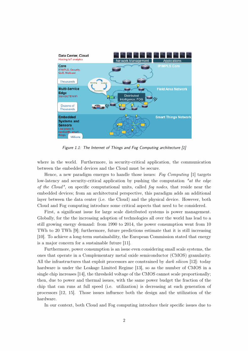
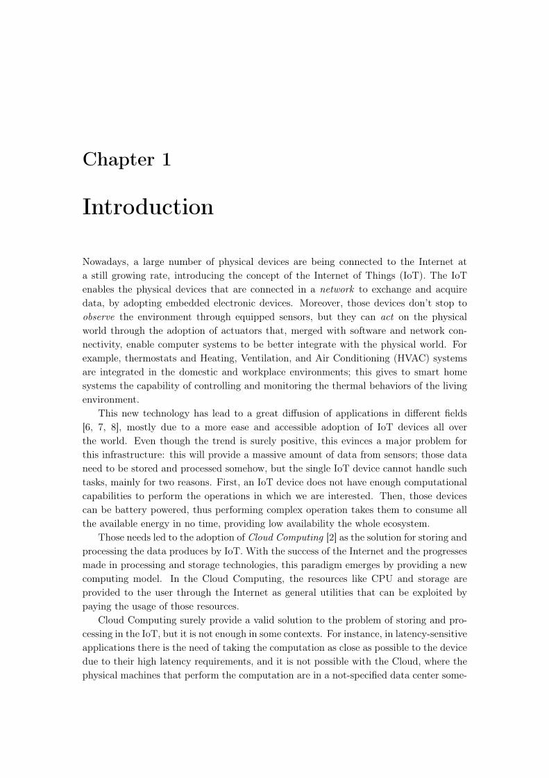
Figure 1.1: The Internet of Things and Fog Computing architecture [1]

where in the world. Furthermore, in security-critical application, the communicationbetween the embedded devices and the Cloud must be secure.

Hence, a new paradigm emerges to handle those issues: Fog Computing [1] targetslow-latency and security-critical application by pushing the computation "at the edgeof the Cloud", on specific computational units, called fog nodes, that reside near theembedded devices; from an architectural perspective, this paradigm adds an additionallayer between the data center (i.e. the Cloud) and the physical device. However, bothCloud and Fog computing introduce some critical aspects that need to be considered.

First, a significant issue for large scale distributed systems is power management.Globally, for the the increasing adoption of technologies all over the world has lead to astill growing energy demand: from 1990 to 2014, the power consumption went from 10TWh to 20 TWh [9]; furthermore, future predictions estimate that it is still increasing[10]. To achieve a long-term sustainability, the European Commission stated that energyis a major concern for a sustainable future [11].

Furthermore, power consumption is an issue even considering small scale systems, theones that operate in a Complementary metal oxide semiconductor (CMOS) granularity.All the infrastructures that exploit processors are constrained by dark silicon [12]: todayhardware is under the Leakage Limited Regime [13], so as the number of CMOS in asingle chip increases [14], the threshold voltage of the CMOS cannot scale proportionally;then, due to power and thermal issues, with the same power budget the fraction of thechip that can runs at full speed (i.e. utilization) is decreasing at each generation ofprocessors [12, 15]. Those issues influence both the design and the utilization of thehardware.

In our context, both Cloud and Fog computing introduce their specific issues due to

2

power consumption.With the introduction of Cloud Computing, it was needed a great amount of com-

putational resources to support the demand of the clients. This has lead the buildingof data centers that requires large spaces and a massive amount of servers. In 2010,Google was hosting 900000 servers, nowadays it is estimated to be more that 1.5 millions[16]. With this great number of machines, it is not trivial to provide energy to the wholeinfrastructure, both in term of the costs and availability [17]. Thus, there is the necessityof guaranteeing that the power consumption of the whole infrastructure will stay undera specified cap.

Moreover, in the context of Fog Computing, there are other power-related issues thatneeds to be tackled. Fog nodes have more computational capabilities that traditionalembedded devices to host all the computations needed by the specific IoT infrastructure,but that does not mean that those nodes are not power constrained. Due to the proximityof the fog nodes to the embedded devices, it is likely that they may be battery-poweredor deployed in a domestic environment, where you cannot dispose of a great amountof energy. Thus, we need to manage the power consumption of fog nodes to guaranteehigh availability of the nodes and the performance objectives of the IoT applications.Furthermore, the possibility of dynamically capping the power demand of the nodes canprovide interesting savings, knowing that we are moving towards a context in whichenergy is provided through smart grids, where the energy cost may vary during the day[18].

To tackle those issues, research is moving towards power management techniques thatoperate directly on the power consumption of a computational units to achieve specificgoals. Specifically, we are interested in guaranteeing that a computing system does notexceed a specific quantity of power consumption. This is the aim of a specific family ofpower management techniques, called power capping [3], where the knobs of the systemare tuned to achieve the desired power cap. Moreover, by exploiting power capping it ispossible to obtain other interesting properties: in a data center it is possible to achieve abetter machine redundancy by managing the capping in such a way that the global powerconsumption of the cluster remains under the cap; in addition, it is possible to boost theperformances of specific servers in a cluster, for example the ones that hosts the mostperformance-critical applications, by orchestrating the power cap of all the nodes whileremaining under the power cap of the cluster.

Then, another critical issue that need to be tackled is the portability of the compu-tation across the Fog and the Cloud. One of the major characteristic of Fog Computingis that fog nodes are heterogeneous by design [1], due to the distinct form factors andenvironments in which they can be deployed. This is an issue considering that the Cloudneeds to exploit the Fog as an extension of its infrastructure at the edge of the network,because if every fog node has its own software stack, it becomes difficult to maintainapplications that need to operate on different environments. Thus, if we need to runapplications on both the Cloud and the Fog, we need an elastic way of deploying portable

3

application from one environment to the other, regardless the underlying architecture.Moreover, we need to consider that Cloud computing operates in a multi-tenancy con-text, where applications run independently from one to the others, while sharing thesame resources.

In this context, containerization techniques are becoming an interesting and stillgrowing trend towards an easy and efficient deployment in a multi tenant environment,thanks to their characteristic of isolation and resource management. By exploiting con-tainers, it is possible to hold an application with all its specific software dependenciesin a single entity and then move it from one environment to the other, without caringabout being in a specific context.

On the other hand, there is an important aspect that needs to be highlighted whenwe are considering services hosted in the Cloud. The Cloud provider needs to satisfy theService level agreements (SLA) stipulated with the client by achieving some performancelevels, defined as Service level objectives (SLO). For example, a web server needs tomaintain a certain number of requests served per seconds and a database needs to providea specific number of queries per second. Indeed, those requirements need to be valid inthe Cloud, and consequently in the Fog; not satisfy them means a loss of profit for theprovider. Moreover, those SLA may change during time. Thus, there is the need of a fine-grained control system that can manage the single application to satisfy the performancerequirements of the latter.

In our context, this is a key aspect that needs to be tackled, because a power cappingthat does not consider the performances of the running applications is not an interestingsolution in a multi-tenant context.

A performance-aware control system that performs power capping is then needed tohandle all the described issues. It needs to manage performance and resource allocationto satisfy the needs of different tenants.

To tackle these problems, we exploit a well known approach used for autonomiccontrol system: the Observe-Decide-Act (ODA) control loop [19]. By adopting thisparadigm, it is possible to rapidly change the system to achieve a specific outcome. Inour case, we are interested in a system that given the current power consumption ofthe machine is able to automatically tune the resources assigned to each container tomeet the power constraints. In this context, we propose DockerCap, a power cappingorchestrator for Docker containers that follow an ODA control loops and a policy-basedsystem to tune the performances of the containers while satisfying the power constraint.

DockerCap is structured as a composition of three major components: the ObserveComponent fetches the current power consumption of the machine and the state of therunning Docker containers; the Decide Component chooses the new allocation of resourcesfor the container by leveraging a combined control and policy based approach; finally, theAct component takes care of performing the physical assignment of the resources to thecontainer through Linux Control Groups [4] based on the decision took in the Decision

4

step.With the control logic, we obtain a capping on the global allocation of the resources

that will guarantee the constraints on the power consumption. Moreover, with the intro-duced policy system it is possible to partition the global allocation of resources, calculatedby the control logic, across all the running containers. The choice of a specific partitionpolicy strongly influences the performance of the container; thus, depending on the per-formance needs, it is possible to choose the preferred partition policy. To highlight thegenerality of the proposed approach, we develop three distinct policies that focus ondistinct outcomes: the first proposed policy splits the resources uniformly across all thecontainers, without caring about the performances; the second policy balances the re-source assignment by relying on a priority assigned to each container; the last proposedpolicy instead, allocates the right amount of resources that are needed to satisfy the SLOof the the containers, following an order of assignment based on the priority associated.

The performance of DockerCap is evaluated in terms of two different metrics: the pre-cision of the capping, and the performances of the containers under power constraints.We consider the precision of the capping as how near the power consumption is withrespect to the desired cap. The obtained results are then compared with the state of theart solution Running Average Power Limit (RAPL) [20].

This thesis is organized as follows:

• in Chapter 2, we present the state of the art and the limitations of the currentworks in the field;

• in Chapter 3, we discuss the problem that DockerCap aims to tackle;

• in Chapter 4 and Chapter 5, we give a high level description and a technical spe-cification of DockerCap;

• in Chapter 6, we present the experimental setup and discuss the results of Docker-Cap

• Finally in Chapter 7, we draw our conclusions and we provide an insight on futuredirections of this work. �

5

Chapter 2

State of the art

From 1990 until today the worldwide power consumption doubled from 10k TWh up to20k TWh; future prediction estimates a consumption of 40k TWh by 2040 [3]. Moreover,the work of Berl et al. [17] highlights that the power-related costs in a data centertakes up to 53% of the whole annual infrastructure budget. Those motivations has leadresearch to produce power management techniques to limit the consumption in the datacenter.

The sections are organized as follows: in section 2.1, we analyze the current powermanagement techniques proposed by the state of the art, especially power capping; insection 2.2, we; in section 2.3 we discuss about the current trends on fog computing bydescribing the requirements and the current works on the field; finally in section 2.4 wediscuss on some other works that proposed similar control-based solution approaches.

2.1 Power capping

The capability to function under power constraints is a major issue due to the limitsof multicore scaling, mostly caused by power and thermal management; the increasingnumber of transistors permit processors to reach their power peak during a limited time,due to the incapability of dissipating the heat produced [12, 13]. Those limitationsintroduced the concept of dark silicon [12]: transistors are not powered or constrainedto operate under their possibilities [15]. Moreover, systems could be subject to powerrestrictions due to energy savings policies in a given time frame.

Researchers have proposed solutions to perform power capping on different systemgranularities: approaches that operates in a context of cluster (i.e. multiple nodes ap-proaches) or on a single machine (i.e. single node approaches).

Regarding multiple nodes approach, Raghavendra et al. [21] proposed a coordinatedpower management architecture that handle distinct single power management solu-tions, whose operate on different granularities on the single machine. Moreover, Wanget al. [22] proposed a Multiple Input-Multiple Output (MIMO) controller that exploitsDynamic Voltage and Frequency Scaling (DVFS) to control the performance and powerconsumption of multiple servers.

These two works proposed interesting approaches based on the control theory tomanage a cluster of servers, but they lack to consider the service level agreement of eachapplication and they are based on an hardware architecture prior to SandyBridge. Inaddition, our work targets power capping on a single node.

Regarding single node approaches, we can identify two different kind of power cappingtechniques: hardware and software based. Nowadays, the main hardware power cappingtechnique is RAPL [20, 5], provided by Intel since SandyBridge processors. From a timeinterval and a power cap passed through Machine Specific Register (MSR), RAPL es-timates the energy budget that will meet the desired power cap. At runtime, it readsvarious low-level hardware events and estimates the power consumption of the specificcomponent (e.g. single core, DRAM, socket). At every time interval, RAPL decidesthe best processors speed and voltage to satisfy the remaining energy budget and setsDVFS. By directly operate on the hardware, RAPL is able to guarantee a stable powerconsumption of the socket in 350ms [23].

Prior to RAPL, research has proposed techniques that exploits manually DVFS.Deng et al. [24] proposed CoScale, a method that coordinates CPU and memory

DVFS under performance constraints. It shows that coordinating multiple componentprovides better results w.r.t. treating each component separately.

The same authors [25] proposed MultiScale, a technique to coordinate DVFS acrossmultiple memory controllers, memory channels and memory devices, still respecting theperformance constraints specified by the user.

Cochran et al. [26] proposed Pack & Cap, a control technique that performs DVFSand thread packing in order to perform under the power budget while maximizing per-formances.

Rangan et al. [27] presents thread motion, a power management technique for chipmultiprocessors that enable movement of threads to adapt to the performance/powerneeds in contrast with the coarse-grained DVFS.

Unfortunately, all the solution that exploits DVFS are limited in a multi-tenant con-text, because whenever the DVFS is performed, the changes on the frequency and voltageaffects the whole socket of the processor, consequently influencing all the cores in it. Thus,all the tenants that resides on the same socket are penalized.

Chen and John [28] introduced a predictive mechanism for multiple resource man-agement in chip multiprocessors. The proposed solution exploits dedicated hardwarecomponents to profile and predict the performances of the threads; it is an interestingapproach but cannot be applied without a specific hardware support.

Unlike hardware, software based approach can tune the resources assigned of the run-ning application, and consequently its performances, to reduce the power consumption.On the other hand, software power capping generally provides a double digit degradation

7

in performances to reach a stable power consumption w.r.t. RAPL [23].Considering software power capping, research has moved towards approaches that

coordinate multiple components, like cpu and memory, to achieve better performance.Hoffmann and Maggio [29] proposed PCP, a general approach that can manage

multiple components to meets the constraints on the power budget while maximizingperformance. It proposes an interesting power capping approach to a general resourcemanagement based on control theory. The major limitation of this work is that all theexperimental evaluations are performed by running a single benchmark at a time. Thisis not interesting in a context where multiple tenants that runs on the same machine,thus competing on the available resources.

Maggio et al. [30] proposed a feedback controller to tailor resource usage online, byactuating on the number of allocated cores and the possible frequencies in embeddeddevices. This work propose an interesting power management approach for embeddeddevices, but it is not feasible in a different architecture, especially in a multi-tenantcontext.

Meisner et al. [31] explored the possibility of using low-power modes to reduce thepower consumed by the primary server components in Online Data-Intensive services.This work propose an interesting study on power modes, but it analyze only a singlefamily of workloads; furthermore without considering other workloads that may run onthe same machine simultaneously.

Nathuji and Schwan [32] proposed VirtualPower, a power management approach tocoordinate each guest VM’s independent power policy to attain desired global objective,by means of hardware and software methods to control power consumption. In ourcontext, this methodology is not applicable, because in general a containerized applicationdoes not implements a power-saving policy, in contrast with virtual machine that hostsan operating system.

Anagnostopolou et al. [33] proposed a power-aware resource allocation algorithm forthe CPU and the memory based on SLA by operating both on the allocation of serviceswithin the cluster and the resource allocated on the single machines. This works focuseson providing an energy-optimal or resource-optimal allocation, while not giving guaranteeon the power consumed. Moreover, it is not clear how they associate the right amountof resources given a SLA.

Felter et al. [34] introduce Power Shifting, a system that reduces the peak powerconsumption of servers by a dynamic allocation of power across the components, whileminimizing the effects on the performances. It highlight how dynamic power budgeting(i.e. adapt the tuning of performances for the specific workload type) can achieve betterresults than static power budgeting.

Li et al. [35] developed an algorithm that control adaptation of processor and memoryto minimizes the energy consumed without exceeding the target performance loss betweenthe two components.

Winter et al. [36] studied the scalability and effectiveness of thread scheduling and

8

power management algorithms on an heterogeneous many-core architecture.Li et al. [37] proposed the algorithm Performance-directed Dynamic and Performance-

directed Static to manage memory and disks; respectively. Those algorithms change thethreshold time in which the component operates until it is moved in idle.

Lastly, there are solutions that focuses on exploiting both hardware and softwarepower capping; Zhang and Hoffmann [23] proposed PUPiL, a hybrid software/hardwarepower capping system. It highlights the aspects of the two types of power capping,hardware and software power capping, and proposes an hybrid capping technique thatprovides the advantages of both. The solution are then compared in terms of timeliness(i.e. the speed with which the cap can be enforced) and efficiency (i.e. the performanceunder the power cap). This work provides the motivation on why performing softwarepower capping is crucial if there is the need of control the performance. Even so, thiswork does not consider the needs of the single application (i.e. SLA), because it providesa general performance improvement w.r.t. RAPL. Moreover, the analyzed workloads areconsidered as generic applications, without making any assumption on the how theseworkloads are managed (e.g. container, virtual machine). This is an important aspectsthat need to be considered, because changing the context implies a different managingof resources: a single container could hosts multiple processes, but the granularity inwhich the resource should be managed is the container and not the process to guaranteea proper isolation of workload.

2.2 Virtualization and Containerization

Virtualization is one of the motivation of the success of Cloud computing: moving fromphysical servers to virtual machines consolidated in less physical servers gives a consid-erable energy saving to cloud providers [2].

This considerable diffusion led hardware producer to include special support for vir-tualization [38], thus driving the current architecture to a virtualized context.

Each virtual machine techniques can be classified w.r.t. the type of hypervisor thatimplements (i.e. the component that runs each single virtual machine): bare-metal orhosted hypervisor.

Bare-metal, or native, or type-1 hypervisors (Figure 2.1a) like Xen [39] hosts multipleoperating systems on the same machine while being the only software that runs directlyon the hardware.

Hosted or type-2 hypervisors (Figure 2.1b) like KVM+Qemu [40, 41] instead hostsmultiple virtual machines while running as an application in the host operating system.

Both of the solutions abstract the physical resources as virtual resources that eachvirtual machine can exploits.

Nowadays, a new paradigm called Containerization (Figure 2.1c) emerges as an al-

9

Figure 2.1: Virtualization and Containerization schema

ternative of Virtualization. Containerization solution like Docker [42] exploits some fea-tures Linux Kernel [43]: by exploiting Linux Control Groups [4] (i.e. cgroups) and LinuxNamespaces [44] it deploys applications inside containers. Each container runs with itslibraries and binaries but it does not have the extra overhead of the guest Operating Sys-tem (OS). With Docker Containers, all the dependencies and libraries are inside a singlecontainer and the common library are shared between the containers, having applicationsthat can be easily deployed.

2.3 Fog Computing

Nowadays, IoT adoption is increasing: Cisco estimates that there will be 50 billion con-nected devices by 2020 [45] while today there are currently 25 billion of devices connec-ted. In this context, due to the low computational capacity of embedded devices, Cloudcomputing is exploited to share, compute and store the data acquired though sensors.Furthermore, for certain types of application, there is the need of strict constraint on thelatency and an higher security; this cannot be achieved by IoT and The Cloud alone,mainly to scaling and proximity issues.

In this context, Fog Computing [1] emerges as a new paradigm as an interplay betweenthe Cloud and IoT. It takes the computation at the edge of the cloud by exploiting fognodes, computational units close to the embedded device, that allows a better scaling,wide geographical distribution, better security and a better support for latency-sensitiveapplications.

10

In the state of the art, there are works that already propose some interesting applic-ations of Fog computing that need to be explored [46, 47].

Zhu et al. [46] highlight some interesting application of Fog computing on improvingweb site performances through compression, caching and some computation on HTMLand stylesheets.

Zhang et al. [47] proposed an higher level of abstraction for the IoT centered arounddata: the Global Data Plane is a data-centric abstraction that focuses on distribution,preservation and protection of the information.

Currently, an issue in Fog Computing is resource management [1], and power consump-tion is not excluded: usually, Fog nodes may be deployed in a domestic environment, thuspower limited, or they may be battery powered. Those aspects highlight the importanceof power management in the Fog Computing.

2.4 Control Theory

Control theory, especially Feedback control, is a well known technique in computer sys-tems [48], in situation in which there is a desired output characteristic.The proposed PI controller is inspired by solution adopted in a context similar to ours[29, 22] and others adopted in different context [49, 50].

Bartolini et al. [49] proposed AutoPro, a runtime system that enhances IaaS cloudswith automated and fine-grained resource provisioning based on performance SLOs. Theydeveloped a PI controller for each VM that provides resource requests based on the SLOand the current performance report. All the resource requests are gathered by a resourcebroker that adapt all the requests to the actual resource availability. The controller isbased on a resource-performance model that binds the VM performance over a giventime window to resource allocation.

Sironi el al. [50] developed ThermOS, an extension for commodity operating systems,which provides dynamic thermal management through feedback control and idle cycleinjection. The controller is synthesized from a linear discrete-time thermal model thatdescribes the temperature behavior.

Both the cited works [49, 50] model the controlled system with an AutoRegressivewith eXogenous input (ARX) model at discrete time steps 2.1.

output(k + 1) = a · output(k) + b · input(k) (2.1)

The parameters a and b can be learned in two different ways: offline [50], throughprevious run and regressions, or online [49], through algorithms like Recursive LeastSquares (RLS). �

11

Chapter 3

Problem definition

This chapter specifies the base concepts needed to discuss about the problem and therespective solution proposed and then introduces the problem that we aim to solve.Furthermore, it gives details about the specific issues that make the problem of powercapping in a containerized environment not trivial to solve.

3.1 Preliminary definitions

In this section, we will introduce the main concept needed to better understand theproblem tackled, defined in section 3.2, and the proposed methodology, introduced inChapter 4.The main concept in which our system relays on is the resource. In general, a resource isseen as an asset that can be exploited to perform a function [51], but our case, we givea more contextualized definition of a resource: a resource is a physical or virtual assetthat an application exploits to perform its own workload. The nature of this resource isbounded to its physical adoption. For example, a process that runs in an operating sys-tem has a finite amount of memory that can exploits; in this case, memory is a resourcefor the process. In the context of containerization, we are interested in the resourcesassociated to a container, that can be observed and/or controlled.Another important aspect that stays on the base of our work is power. The meaning givento the term power is based on its definition in physic: power is the rate of doing work, asthe amount of energy consumed per unit time. More specifically, we focus on the powerconsumption of a single machine, the one that runs an instance of the orchestrator. Oneof the main aspect in which we are interested in is the possibility of performing powercapping, a power management technique that aims to keep at a stable value the powerconsumption of the whole considered system. The amount of power consumption thatthis technique wants to guarantee is called power cap.Moreover, we consider performance as a manner to evaluate the current running con-tainers. In general, we cannot give a specific metric for the performances, because eachworkload can be evaluated by different point of views. This vision is represented bygiving a performance metric for each container. By looking to the performance metrics,we can evaluate the current computation performed by the containers.

There are some contextes in which a container needs to keep a specific level of perform-ances. For instance, a single instance of a database must guarantee a specific number ofquery served per second, or a web server must provide a defined number of requests persecond. In the context of services hosted on the Cloud, those constraints on perform-ances are defined in the Service Level Agreements. They are part of a service contractwhere aspects of the service are agreed, like quality, scope and responsibilities. Thoserequirements need to be satisfied by the provider; if it doesn’t happen, there is a loss ofprofit for the provider. Specifically, we focus on performance requirements, that in theSLA are defined as that Service Level Objectives. Those objectives are a combination ofQuality of Service measures that produces an achievement value.

3.2 Problem statement

Our goal is to perform power capping in a containerized context; furthermore, we wantto have control over the performance of the running container. To be able to achieve thedesired results, there is the need of an orchestrator for container that, depending on theselected policy, can control the resources of the running containers in such a way thatthe cap is guaranteed and the performances are controlled.First of all, to achieve the desired goal, we need to better highlight the criticality thatneed to be tackled by providing such solution.To perform power capping, we are interested in the relationship between the power con-sumption of the system and the resources assigned to the running containers. Dependingon the workload, we can obtain a different dependency between the power consumptionand a given resource. This relationship does not hold for all the types of workloads,because each application performs different operation, thus it exploits the underlyinghardware differently. For example, for a CPU-bound workload the relationship betweenthe CPU quota assigned to the container influences the power consumption of a machineproportionally, because with a higher quota, the application can perform more operationsduring the same period; this influences the utilization of the hardware, and consequen-tially the power consumption (Figure 3.1). This highlight the importance of choosingthe right resources that influences the power consumption of the system.Another important issue that need to be considered is the relationship between the

resources and the performances of each workload. Giving a higher amount of resources,the workload can better exploits the hardware to perform its operations. For instance, ifa CPU-bound workload has a higher CPU quota, then it will perform more operationsduring the time period, thus it will provides higher performances (Figure 3.2). Then,considering the two described relationship, we need to focus on the problem that we wantto solve: capping power consumption while providing control over resources. The choiceof the right amount of resources that satisfy the goal is not trivial: on the one hand,we want to limit the power consumption of the machine; on the other hand, we want tocontrol the performances of the tenants. Unfortunately, those two metrics shows opposite

13

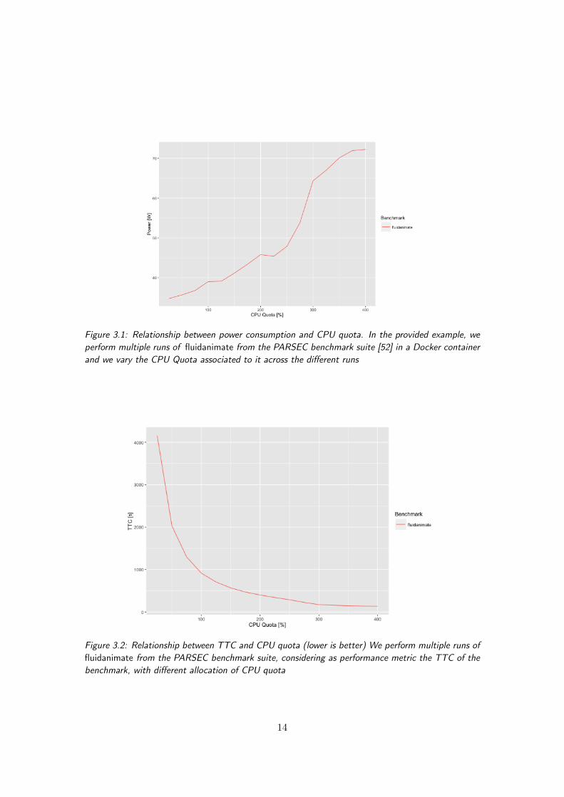
Figure 3.1: Relationship between power consumption and CPU quota. In the provided example, weperform multiple runs of fluidanimate from the PARSEC benchmark suite [52] in a Docker containerand we vary the CPU Quota associated to it across the different runs

Figure 3.2: Relationship between TTC and CPU quota (lower is better) We perform multiple runs offluidanimate from the PARSEC benchmark suite, considering as performance metric the TTC of thebenchmark, with different allocation of CPU quota

14

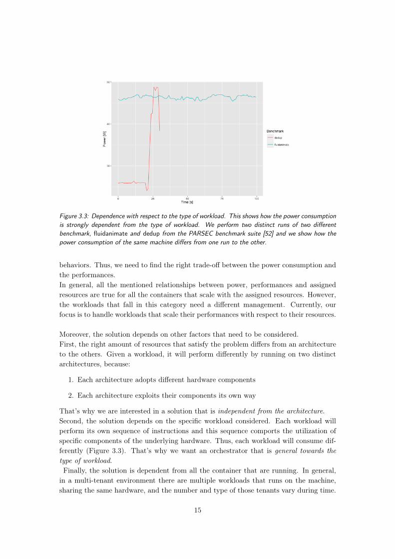
Figure 3.3: Dependence with respect to the type of workload. This shows how the power consumptionis strongly dependent from the type of workload. We perform two distinct runs of two differentbenchmark, fluidanimate and dedup from the PARSEC benchmark suite [52] and we show how thepower consumption of the same machine differs from one run to the other.

behaviors. Thus, we need to find the right trade-off between the power consumption andthe performances.In general, all the mentioned relationships between power, performances and assignedresources are true for all the containers that scale with the assigned resources. However,the workloads that fall in this category need a different management. Currently, ourfocus is to handle workloads that scale their performances with respect to their resources.

Moreover, the solution depends on other factors that need to be considered.First, the right amount of resources that satisfy the problem differs from an architectureto the others. Given a workload, it will perform differently by running on two distinctarchitectures, because:

1. Each architecture adopts different hardware components

2. Each architecture exploits their components its own way

That’s why we are interested in a solution that is independent from the architecture.Second, the solution depends on the specific workload considered. Each workload willperform its own sequence of instructions and this sequence comports the utilization ofspecific components of the underlying hardware. Thus, each workload will consume dif-ferently (Figure 3.3). That’s why we want an orchestrator that is general towards thetype of workload.Finally, the solution is dependent from all the container that are running. In general,

in a multi-tenant environment there are multiple workloads that runs on the machine,sharing the same hardware, and the number and type of those tenants vary during time.

15

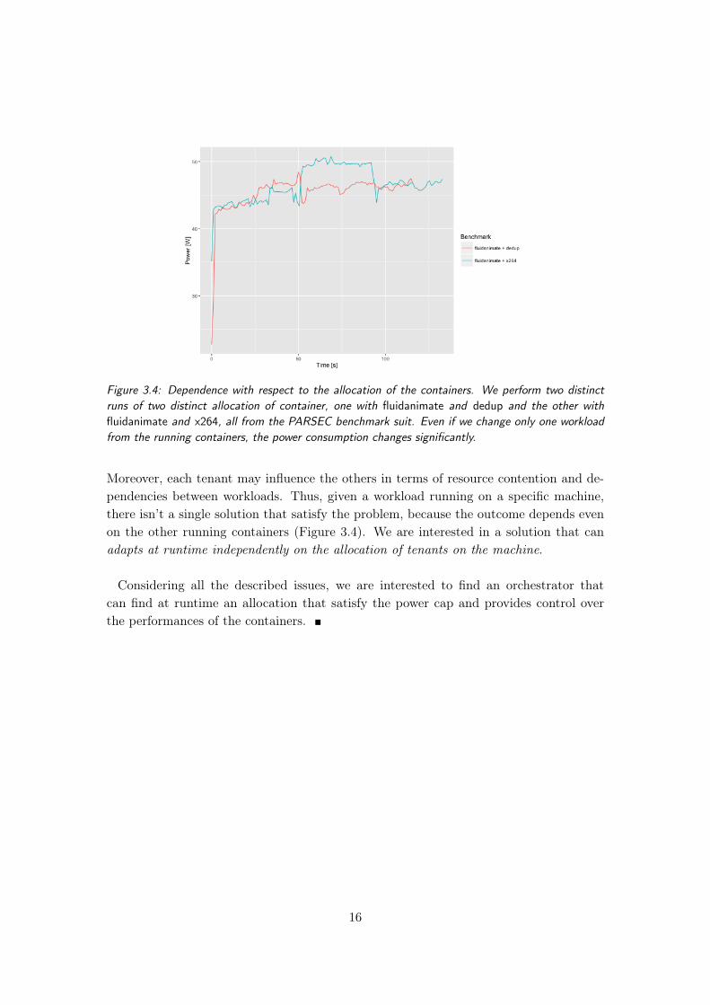
Figure 3.4: Dependence with respect to the allocation of the containers. We perform two distinctruns of two distinct allocation of container, one with fluidanimate and dedup and the other withfluidanimate and x264, all from the PARSEC benchmark suit. Even if we change only one workloadfrom the running containers, the power consumption changes significantly.

Moreover, each tenant may influence the others in terms of resource contention and de-pendencies between workloads. Thus, given a workload running on a specific machine,there isn’t a single solution that satisfy the problem, because the outcome depends evenon the other running containers (Figure 3.4). We are interested in a solution that canadapts at runtime independently on the allocation of tenants on the machine.

Considering all the described issues, we are interested to find an orchestrator thatcan find at runtime an allocation that satisfy the power cap and provides control overthe performances of the containers. �

16

Chapter 4

Proposed methodology

After the definition of the problem on which this work is focused, we now present themethodology behind DockerCap. In this chapter, we focus on the details of the approachof DockerCap, presenting how each single step is designed to guarantee a specific goal.The chapter is organized as follows: in Section 4.1 we give a general overview of Docker-Cap; in Section 4.2 we define the problem tackled in the Observe Phase; in Section 4.3we give an overview on the decision problem and we will discuss in detail the choicesmade in each of the subphases; finally in section 4.4 we present the Actuation phase anddiscuss about some enhancements exploitable.

4.1 DockerCap in a nutshell

DockerCap is a power capping orchestrator for Docker containers: it manages at runtimethe resources assigned to the running containers to meet requirements of power consump-tion and of performances.First, it guarantees that the power consumption will not exceed the desired cap: this isthe main objective of a power capping system.Second, given the constraint on resources to satisfy the power cap, it partitions andallocates the right amount of resources that allows some containers to satisfy their per-formance requirements: while performing power capping, the system will be underused.Under those constraints, it is not always possible to satisfy the performance requirementof all the containers. That’s why we need to define policies to tune the performances ofthe containers to achieve an goal.

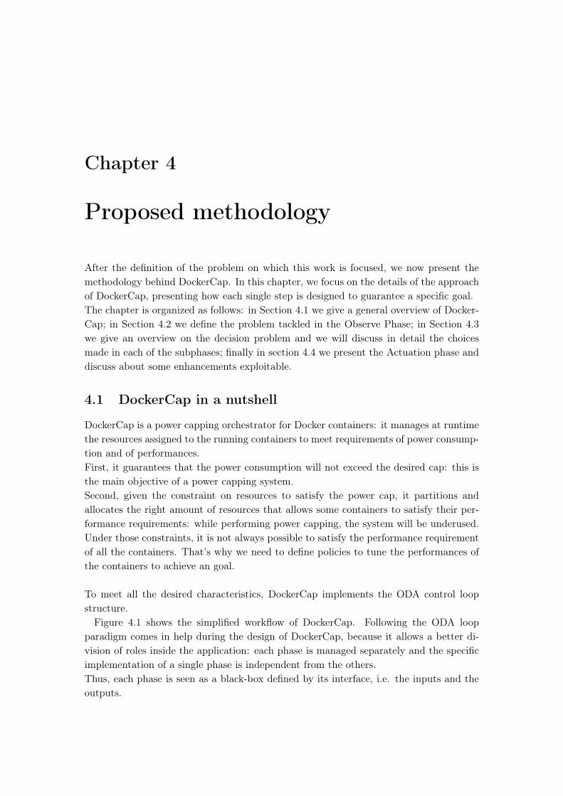
To meet all the desired characteristics, DockerCap implements the ODA control loopstructure.Figure 4.1 shows the simplified workflow of DockerCap. Following the ODA loop

paradigm comes in help during the design of DockerCap, because it allows a better di-vision of roles inside the application: each phase is managed separately and the specificimplementation of a single phase is independent from the others.Thus, each phase is seen as a black-box defined by its interface, i.e. the inputs and theoutputs.

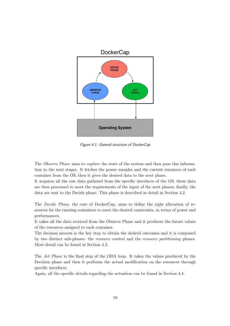
Figure 4.1: General structure of DockerCap

The Observe Phase aims to capture the state of the system and then pass this informa-tion to the next stages. It fetches the power samples and the current resources of eachcontainer from the OS, then it gives the desired data to the next phase.It acquires all the raw data gathered from the specific interfaces of the OS; those dataare then processed to meet the requirements of the input of the next phases; finally, thedata are sent to the Decide phase. This phase is described in detail in Section 4.2.

The Decide Phase, the core of DockerCap, aims to define the right allocation of re-sources for the running containers to meet the desired constraints, in terms of power andperformances.It takes all the data received from the Observe Phase and it produces the future valuesof the resources assigned to each container.The decision process is the key step to obtain the desired outcomes and it is composedby two distinct sub-phases: the resource control and the resource partitioning phases.More detail can be found in Section 4.3.

The Act Phase is the final step of the ODA loop. It takes the values produced by theDecision phase and then it performs the actual modification on the resources throughspecific interfaces.Again, all the specific details regarding the actuation can be found in Section 4.4.

18

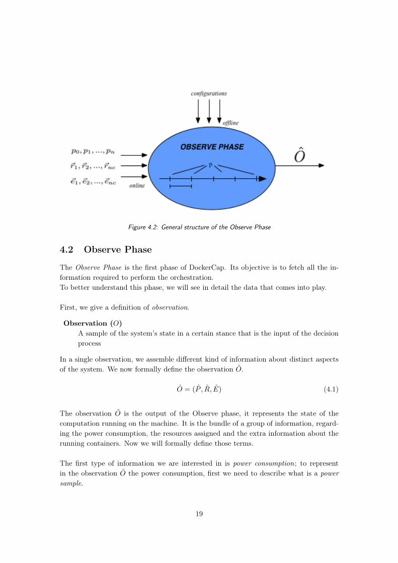
Figure 4.2: General structure of the Observe Phase

4.2 Observe Phase

The Observe Phase is the first phase of DockerCap. Its objective is to fetch all the in-formation required to perform the orchestration.To better understand this phase, we will see in detail the data that comes into play.

First, we give a definition of observation.

Observation (O)A sample of the system’s state in a certain stance that is the input of the decisionprocess

In a single observation, we assemble different kind of information about distinct aspectsof the system. We now formally define the observation O.

O = (P , R, E) (4.1)

The observation O is the output of the Observe phase, it represents the state of thecomputation running on the machine. It is the bundle of a group of information, regard-ing the power consumption, the resources assigned and the extra information about therunning containers. Now we will formally define those terms.

The first type of information we are interested in is power consumption; to representin the observation O the power consumption, first we need to describe what is a powersample.

19

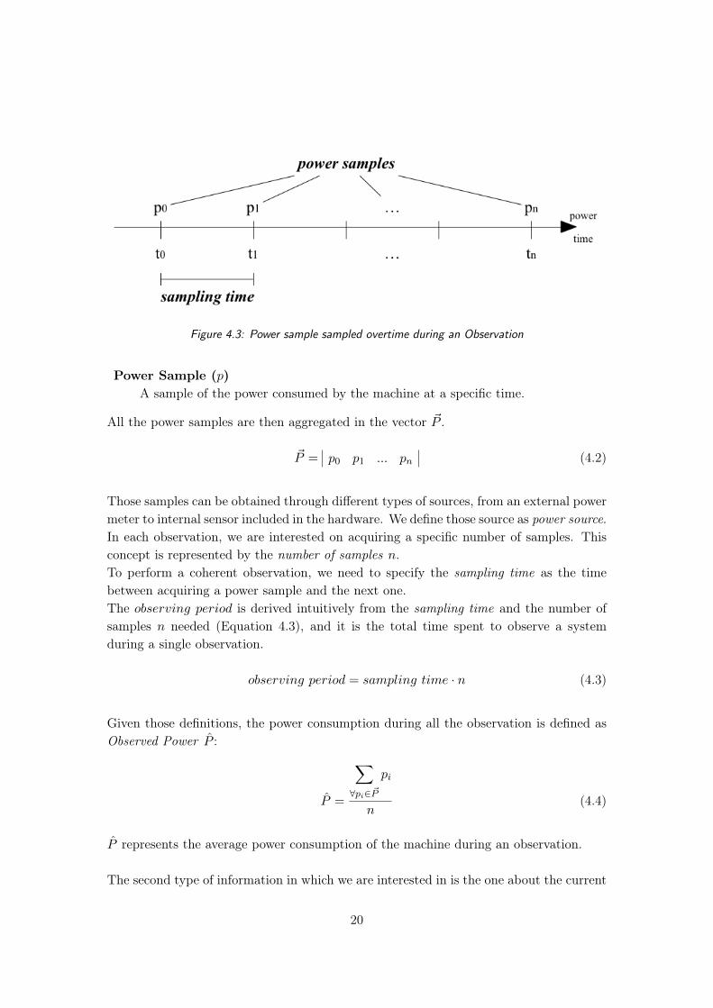
Figure 4.3: Power sample sampled overtime during an Observation

Power Sample (p)A sample of the power consumed by the machine at a specific time.

All the power samples are then aggregated in the vector ~P .

~P = p0 p1 ... pn (4.2)

Those samples can be obtained through different types of sources, from an external powermeter to internal sensor included in the hardware. We define those source as power source.In each observation, we are interested on acquiring a specific number of samples. Thisconcept is represented by the number of samples n.To perform a coherent observation, we need to specify the sampling time as the timebetween acquiring a power sample and the next one.The observing period is derived intuitively from the sampling time and the number ofsamples n needed (Equation 4.3), and it is the total time spent to observe a systemduring a single observation.

observing period = sampling time · n (4.3)

Given those definitions, the power consumption during all the observation is defined asObserved Power P :

P =

∑∀pi∈~P

pi

n(4.4)

P represents the average power consumption of the machine during an observation.

The second type of information in which we are interested in is the one about the current

20

resource of each container.We define the set of all the running container C. For every running container c, we wantto obtain all the resources assigned to it. We define rc as the vector containing all theobserved resources of container c.

~rc = r1 r2 ... rnr ∀c ∈ C (4.5)

Where nr is the cardinality of the considered resources. For example, the amount ofmemory assigned to each container is considered as a resource, and if we are interested inonly that resource, the cardinality nr is equal to 1. Those resources are fetched throughinterfaces that are specific for each type of the resources.To sum up all the information about the resources for each container, we aggregate allthe vectors rc in a single representation R.

~rc ∈ R ∀c ∈ C (4.6)

Where nc is the cardinality of C, the number of running containers. This single repres-entation R contains all the current allocation of resources for all the containers. Thoseinformation will be exploited later by the Decision step.

The last information needed is the extra data about the running containers. This in-formation is represented by ~ec, and it contains all the data of the container c that arenot resources. All the extra information on the containers are then grouped in a singlerepresentation E. For example, for each container, we are interested in knowing its id tobetter identify the workload and performing a proper actuation on the container. Thisid is part of ~ec, as an information about a container that is not a resource.

Once we obtain the observed power P , the current resource allocation R and the ex-tra information on the container E, we finally have the observation O. This bundleis then passed to the next phase, the Decide Phase, where those information will beprocessed to produce the new allocation of resources.

4.3 Decide Phase

The Decide Phase is the second phase of the workflow of DockerCap. Its goal is tofind the right allocation of resources that will be assigned to each container, to meetthe constraints on power and performances. The problem is to find the best trade-offbetween the power constraints and the desired performances by resource management.This trade-off between power consumption and performances is not balanced, becausewe prioritize the constraint on the first over the latter. The first priority of DockerCap isto guarantee the power cap; then, under the power constraint, it takes into consideration

21

Figure 4.4: General structure of the Decide Phase

the performances of each container by trying to find an allocation of resources that canprovide throughput. This must be performed at runtime.First, we need to specify the available information in this step; we can classify the inform-ation in two different types: the information available at runtime, and the ones providedoffline.On the one hand, the available information at runtime are the ones received by the Ob-serve phase, i.e. the observation O.On the other hand, the offline information depends on the needs of the specific decisionprocess. For instance, some policies need to know the SLO of the running containers, ifexists, to better tune the resources with respect to their requirements. The only offlineinformation that is mandatory is the value of power capping.

We divided the decision process in two separate but yet dependent subphases. Eachsubphase is designed to be modular; thus, it is possible to add and change the policy tomeet the desired outcome.The first subphase is Resource Control : it focuses on solving the primary issue of Docker-Cap, i.e. finding an allocation of resources that satisfy the power cap. The proposedpolicies of the resource control exploits control theory techniques to provide stability tothe power consumption with respect to the power cap.The second subphase is Resouce Partitioning : it handles the partitioning of the resourcesto satisfy the constraints on the performances of each container. Since the previoussupbhase provides the global allocation of resources that with satisfy the power cap, weneed to partition this global assignment across all the running containers. Altering theresources allocated consequently change the performance of the running containers.

In the next subsections, we describe in detail both the subphases.

22

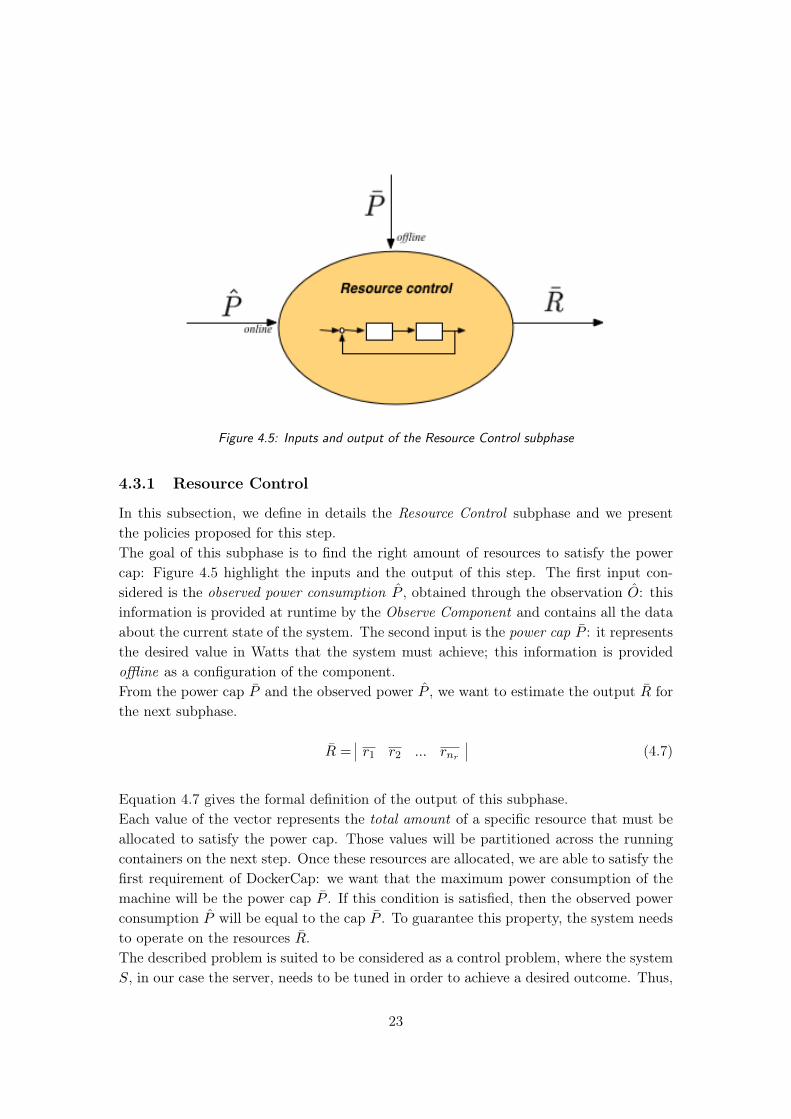
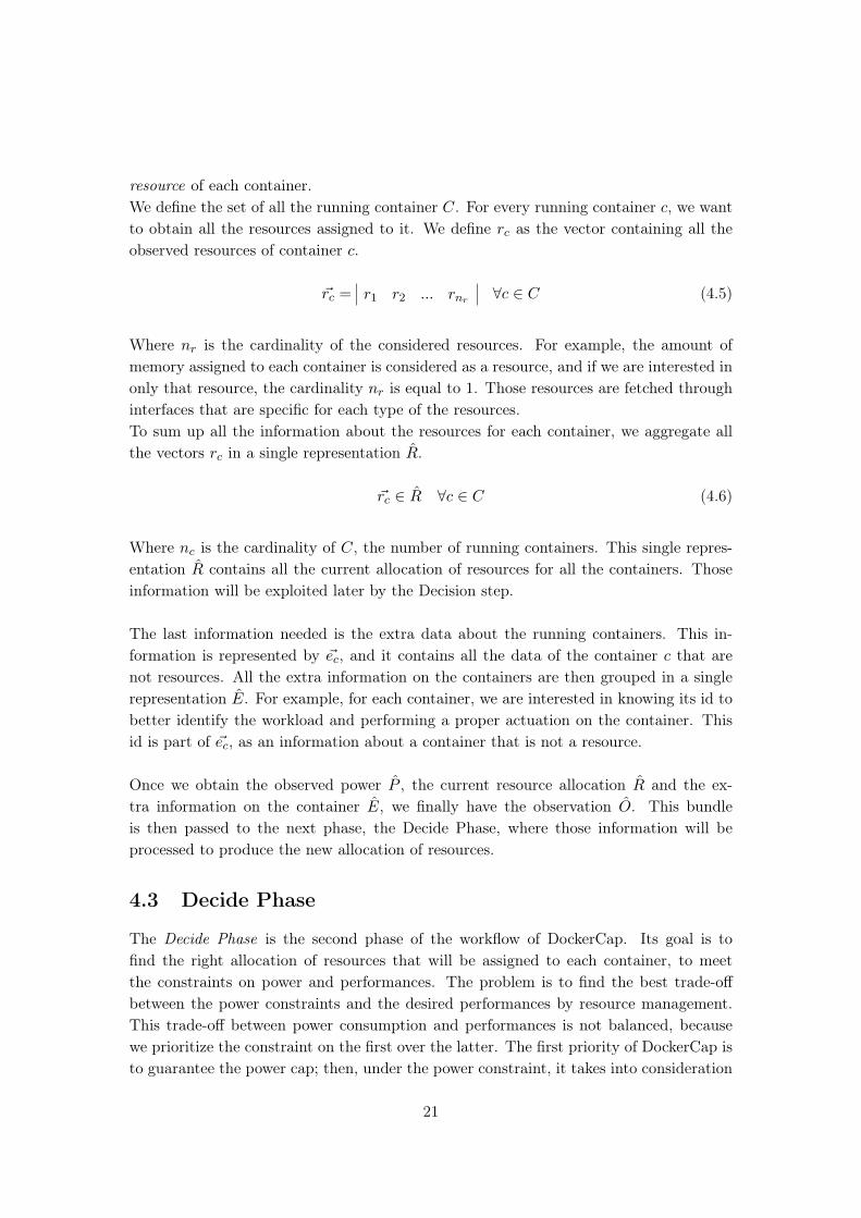
Figure 4.5: Inputs and output of the Resource Control subphase

4.3.1 Resource Control

In this subsection, we define in details the Resource Control subphase and we presentthe policies proposed for this step.The goal of this subphase is to find the right amount of resources to satisfy the powercap: Figure 4.5 highlight the inputs and the output of this step. The first input con-sidered is the observed power consumption P , obtained through the observation O: thisinformation is provided at runtime by the Observe Component and contains all the dataabout the current state of the system. The second input is the power cap P : it representsthe desired value in Watts that the system must achieve; this information is providedoffline as a configuration of the component.From the power cap P and the observed power P , we want to estimate the output R forthe next subphase.

R = r1 r2 ... rnr (4.7)

Equation 4.7 gives the formal definition of the output of this subphase.Each value of the vector represents the total amount of a specific resource that must beallocated to satisfy the power cap. Those values will be partitioned across the runningcontainers on the next step. Once these resources are allocated, we are able to satisfy thefirst requirement of DockerCap: we want that the maximum power consumption of themachine will be the power cap P . If this condition is satisfied, then the observed powerconsumption P will be equal to the cap P . To guarantee this property, the system needsto operate on the resources R.The described problem is suited to be considered as a control problem, where the systemS, in our case the server, needs to be tuned in order to achieve a desired outcome. Thus,

23

Figure 4.6: Feedback control loop exploited in the Resource Control phase

we decided to exploit feedback control techniques [48] to tackle this problem.

A model of the machine is then needed if we want to obtain a controller for our sys-tem. The first model that we considered is an ARX model, based from other works thathandle a similar problem in a different context [49, 50]. The formulation of the problemis as follows:

p(k + 1) = a · p(k) + b · r(k) (4.8)

The values p(k) and p(k+ 1) represent the power consumption of the machine at time kand k+1 respectively. The value r(k) represents the total amount of resource assigned tothe machine. For simplicity, we consider r(k) as a single resource but approach remainsfeasible even considering multiple resources, as the same problem can be formulated asa multiple-input and single-output by considering multiple resource in the Equation 4.8.The parameters a and b are the weights of each component in the model. Those para-meters can be obtained in two different ways: offline or online.Offline methods usually imply some kind of regression, like Least Squares (LS), performedon a set of data acquired through multiple runs of different benchmarks.Online method, instead, are exploited in contexts in which it is not useful or possible tolearn those parameters by a preliminary characterization. Usually those methods exploittechniques like RLS or the Kalman filter [53].

Our goal is to find the right value of r(k), the previous defined output of the phaseR that will provide takes the power consumption of the machine as close as possible tothe power cap. Thus, we want to minimize the error e(k):

e(k) = p(k)− P (4.9)

Figure 4.6 represents the structure of the control loop adopted by the resource controlphase.Once we know the behavior of S, the next step is to find the formulation of the controller

24

C. To do that, we apply the Z-transformation [54] to the model of the machine (Equation4.8) to change the problem from the time domain to the frequency domain.

z · P (z) = a · P (z) + b ·R(z) (4.10)

From Equation 4.11, we obtain the system transfer function S(z).

S(z) =P (z)

R(z)=

b

z − a(4.11)

The controller C(z) is introduced in a feedback control loop to control the resourcesassigned to the system to meet the power cap. Considering that we adopting a feedbackcontrol system, we are interested in a stable feedback control loop, because we don’twant the power consumption to diverge from the power cap P , but we want it to staynear the reference power. Thus, we impose the transfer function of the feedback controlloop stable. We define the loop transfer function as a first-order transfer function witha single pole in p. To achieve an asymptotically stable and not oscillating control, thevalue of p must be between the interval (0, 1).

L(z) =C(z) · S(z)

1 + C(z) · S(z),

1− pz − p

p ∈ (0, 1) (4.12)

By combining Equation 4.11 and Equation 4.12, we obtain the transfer function of thecontroller C(z).

C(z) =(1− p) · (z − a)

b · (z − 1),R(z)

E(z)p ∈ (0, 1) (4.13)

Where E(z) is the error e(k) in the frequency domain.Finally, by applying the inverse Z-Transform and a time shift, we obtain the formulationof the controller in the time domain.

r(k) = r(k − 1) +1− pb· (e(k)− a · e(k − 1)) (4.14)

With this formulation, we have a controller that can give us the value of the resources inwhich we are interested in.

This first solution can be simplified if we make some consideration about our domain.We need to notice that there is a major difference between our work and the others men-tioned [49, 50]: power consumption does not follow a transient behavior, like energy andtemperature. A change in the resource associated to a container implies an immediatereaction to the power consumption of the machine, and that value is independent from

25

the previous one.In order to consider this phenomenon, we explore a model for the machine that is dif-ferent from the ARX(1). We proposed a simpler linear model that depends only on theassigned resources, as follows:

p(k + 1) = b · r(k) (4.15)

This model can be seen as a special case of the ARX model with a = 0. Thus, if weperform the same steps done from the previous model, we obtain a simpler version of thecontroller:

r(k) = r(k − 1) +1− pb· e(k) (4.16)

In chapter 6 we compare the two proposed methodology to find the best controller thatfits our context.

To conclude, with the feedback controller introduced, we are able to exploit a controllogic that provides the total amount of resource that needs to be allocated from theobserved power consumption.The next subsection handles the problem of partitioning the resources across the runningcontainers.

4.3.2 Resource Partitioning

In this subsection, we define the Resource Partitioning phase and we introduce thepolicies proposed to tackle the problem of performance in different ways.

The goal of this subphase is to find the best resource partitioning that optimizes aspecific metric. This metric indeed influences the selection of the partitioning policy.For instance, if the provided metric represents the specific performances of the workloadneeds to be treated differently with respect to another one that is more general, like theHardware Performance Counters (HPC). Figure 4.7 highlight the inputs and the outputof the phase.The first input is the results obtained from the Resource Control subphase, thus the

available resources R that this phase need to partition. This information is acquiredonline, as provided by the previous subphase. The other inputs, the one obtained offline,are policy-specific informations and the configuration of the partitioning subphase .Given the resource R and others offline information, this phase must produce a parti-tioning of resources.

~rcapc = rcap1 rcap2 ... rcapnr ∀c ∈ C (4.17)

26

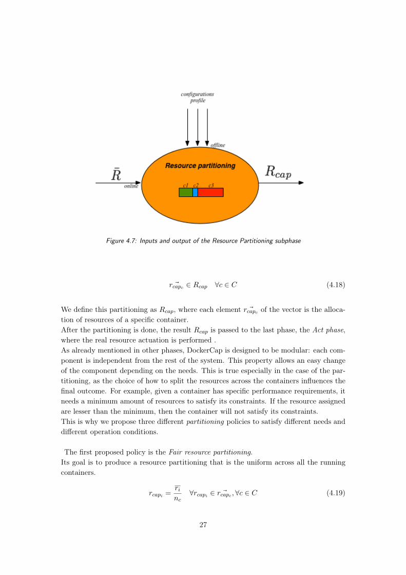
Figure 4.7: Inputs and output of the Resource Partitioning subphase

~rcapc ∈ Rcap ∀c ∈ C (4.18)

We define this partitioning as Rcap, where each element ~rcapc of the vector is the alloca-tion of resources of a specific container.After the partitioning is done, the result Rcap is passed to the last phase, the Act phase,where the real resource actuation is performed .As already mentioned in other phases, DockerCap is designed to be modular: each com-ponent is independent from the rest of the system. This property allows an easy changeof the component depending on the needs. This is true especially in the case of the par-titioning, as the choice of how to split the resources across the containers influences thefinal outcome. For example, given a container has specific performance requirements, itneeds a minimum amount of resources to satisfy its constraints. If the resource assignedare lesser than the minimum, then the container will not satisfy its constraints.This is why we propose three different partitioning policies to satisfy different needs anddifferent operation conditions.

The first proposed policy is the Fair resource partitioning.Its goal is to produce a resource partitioning that is the uniform across all the runningcontainers.

rcapi =rinc

∀rcapi ∈ ~rcapc ,∀c ∈ C (4.19)

27

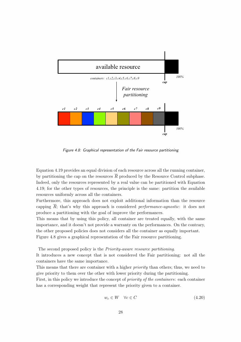
Figure 4.8: Graphical representation of the Fair resource partitioning

Equation 4.19 provides an equal division of each resource across all the running container,by partitioning the cap on the resources R produced by the Resource Control subphase.Indeed, only the resources represented by a real value can be partitioned with Equation4.19; for the other types of resources, the principle is the same: partition the availableresources uniformly across all the containers.Furthermore, this approach does not exploit additional information than the resourcecapping R; that’s why this approach is considered performance-agnostic: it does notproduce a partitioning with the goal of improve the performances.This means that by using this policy, all container are treated equally, with the sameimportance, and it doesn’t not provide a warranty on the performances. On the contrary,the other proposed policies does not considers all the container as equally important.Figure 4.8 gives a graphical representation of the Fair resource partitioning.

The second proposed policy is the Priority-aware resource partitioning.It introduces a new concept that is not considered the Fair partitioning: not all thecontainers have the same importance.This means that there are container with a higher priority than others; thus, we need togive priority to them over the other with lower priority during the partitioning.First, in this policy we introduce the concept of priority of the containers: each containerhas a corresponding weight that represent the priority given to a container.

wc ∈W ∀c ∈ C (4.20)

28

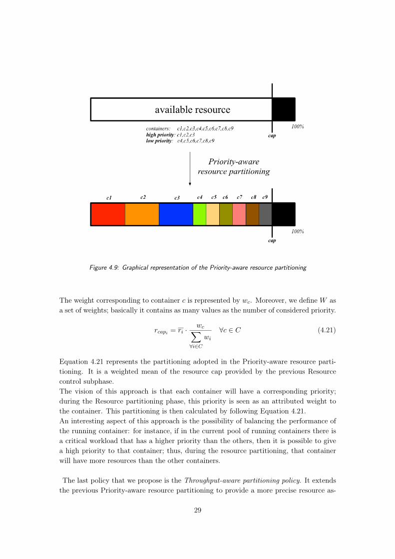
Figure 4.9: Graphical representation of the Priority-aware resource partitioning

The weight corresponding to container c is represented by wc. Moreover, we define W asa set of weights; basically it contains as many values as the number of considered priority.

rcapi = ri ·wc∑

∀i∈Cwi

∀c ∈ C (4.21)

Equation 4.21 represents the partitioning adopted in the Priority-aware resource parti-tioning. It is a weighted mean of the resource cap provided by the previous Resourcecontrol subphase.The vision of this approach is that each container will have a corresponding priority;during the Resource partitioning phase, this priority is seen as an attributed weight tothe container. This partitioning is then calculated by following Equation 4.21.An interesting aspect of this approach is the possibility of balancing the performance ofthe running container: for instance, if in the current pool of running containers there isa critical workload that has a higher priority than the others, then it is possible to givea high priority to that container; thus, during the resource partitioning, that containerwill have more resources than the other containers.

The last policy that we propose is the Throughput-aware partitioning policy. It extendsthe previous Priority-aware resource partitioning to provide a more precise resource as-

29

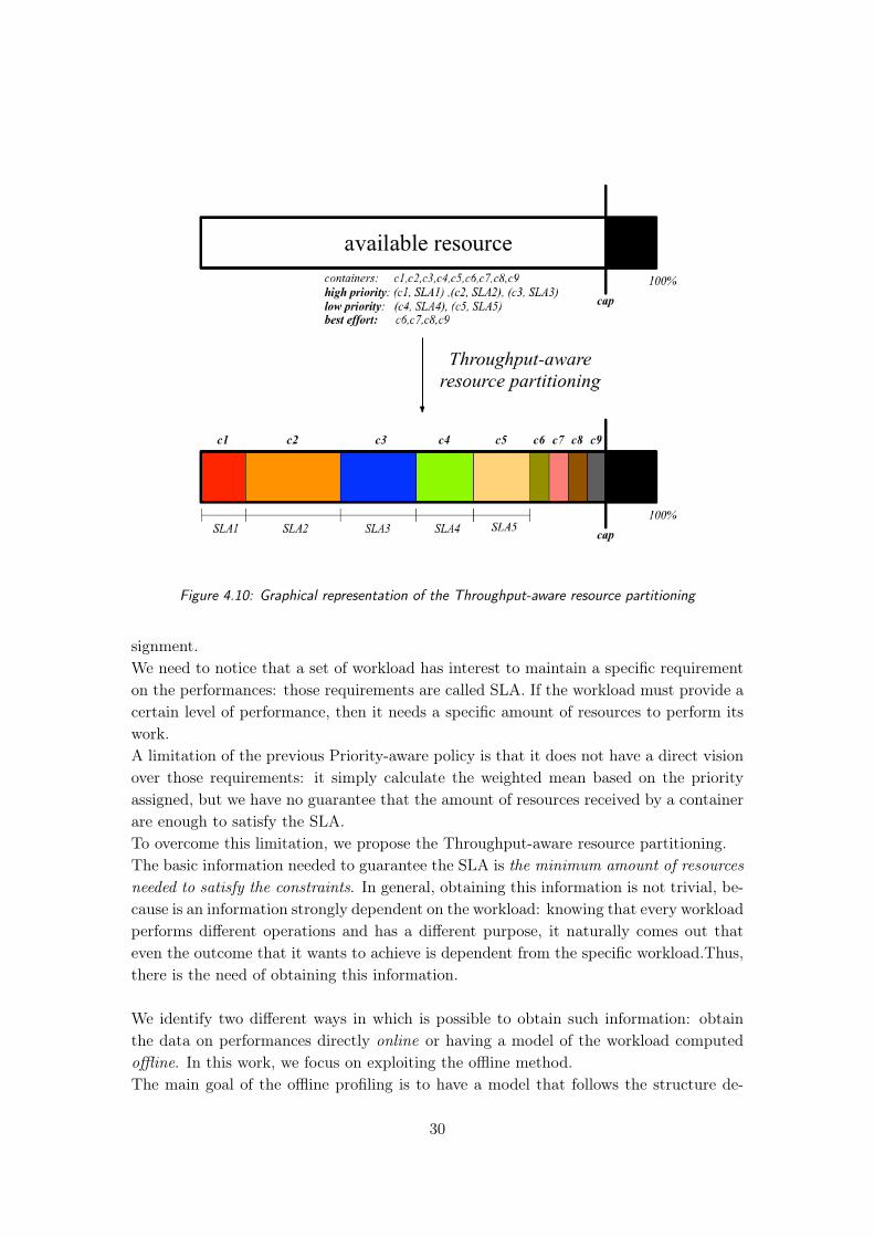
Figure 4.10: Graphical representation of the Throughput-aware resource partitioning

signment.We need to notice that a set of workload has interest to maintain a specific requirementon the performances: those requirements are called SLA. If the workload must provide acertain level of performance, then it needs a specific amount of resources to perform itswork.A limitation of the previous Priority-aware policy is that it does not have a direct visionover those requirements: it simply calculate the weighted mean based on the priorityassigned, but we have no guarantee that the amount of resources received by a containerare enough to satisfy the SLA.To overcome this limitation, we propose the Throughput-aware resource partitioning.The basic information needed to guarantee the SLA is the minimum amount of resourcesneeded to satisfy the constraints. In general, obtaining this information is not trivial, be-cause is an information strongly dependent on the workload: knowing that every workloadperforms different operations and has a different purpose, it naturally comes out thateven the outcome that it wants to achieve is dependent from the specific workload.Thus,there is the need of obtaining this information.

We identify two different ways in which is possible to obtain such information: obtainthe data on performances directly online or having a model of the workload computedoffline. In this work, we focus on exploiting the offline method.The main goal of the offline profiling is to have a model that follows the structure de-

30

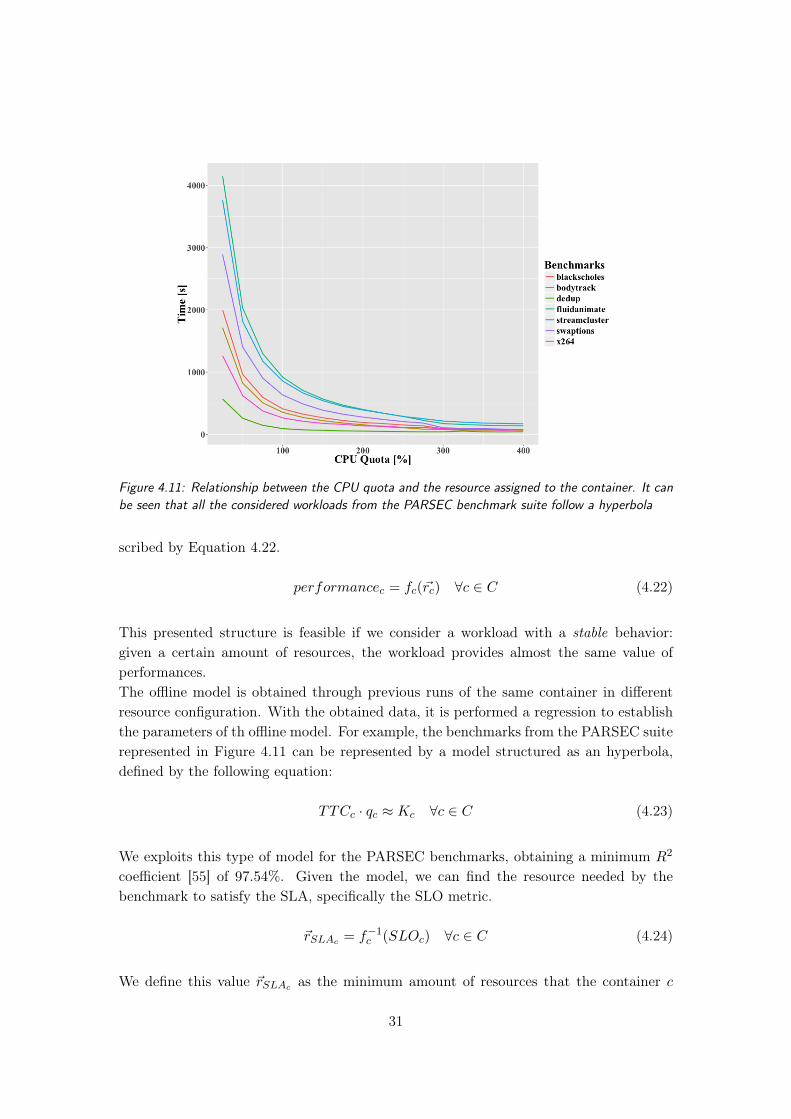
Figure 4.11: Relationship between the CPU quota and the resource assigned to the container. It canbe seen that all the considered workloads from the PARSEC benchmark suite follow a hyperbola

scribed by Equation 4.22.

performancec = fc(~rc) ∀c ∈ C (4.22)

This presented structure is feasible if we consider a workload with a stable behavior:given a certain amount of resources, the workload provides almost the same value ofperformances.The offline model is obtained through previous runs of the same container in differentresource configuration. With the obtained data, it is performed a regression to establishthe parameters of th offline model. For example, the benchmarks from the PARSEC suiterepresented in Figure 4.11 can be represented by a model structured as an hyperbola,defined by the following equation:

TTCc · qc ≈ Kc ∀c ∈ C (4.23)

We exploits this type of model for the PARSEC benchmarks, obtaining a minimum R2

coefficient [55] of 97.54%. Given the model, we can find the resource needed by thebenchmark to satisfy the SLA, specifically the SLO metric.

~rSLAc = f−1c (SLOc) ∀c ∈ C (4.24)

We define this value ~rSLAc as the minimum amount of resources that the container c

31

must have available to satisfy its SLA.Moreover, by exploiting a priority assignment method like the one described for thePriority-aware policy, and with the allocation ~rSLAc for each container, we can introducethe Throughput-aware resource partitioning policy.First, we need to specify that each container must receive a minimum amount of resources,so that the whole capping process should not terminate a running container.Knowing that each container has its own priority, we need to assign the right amount ofresources first to the ones with the highest priority. Then the same process is repeatedfor all the priorities of the containers with specified SLA.Furthermore, it may happen to have containers without a defined SLA. In this case, wehave defined a special priority, known has best effort, that is treated separately by theThroughput-aware policy.All the containers with the best effort policies will receive the resources leavings of theother priorities, partitioned by following the Fair resource partitioning policy. This ispossible because we don’t necessarily allocate all the available resources with the previousassignments, because each container with a defined SLO demand a specific amount ofresources.On the other hand, there are cases in which, for a given priority, there are not sufficientresources to satisfy all the SLO of the containers with that priority. In this case, it isperformed a Fair resource assignment across all the containers with that priority. Allthe containers that have a lower priority, included the best effort, will remain with theminimum quantity of resources guaranteed by the partitioning policy.Figure 4.10 shows a graphical representation of a run of the Throughput-aware resourcepartitioning.

4.4 Act Phase

The Act Phase is the last phase of the workflow of DockerCap. Its goal is to performthe physical allocation of the resources given the allocation of resources produces by theDecide Phase.Performing the actuation on the resources is dependent from the type of resource thatwe are managing.That is why we introduce the concept of Actuation Interfaces.

Actuation Interface(A)A software interface that takes care of performing the physical change on a specifictype of resource

In addition to the physical changes on the resources, each Actuation Interface takes careof normalizing the computed resource value for the specific resource.Thus, given an allocation of resources Rcap, we associate each resource value rcapi to itsspecific Actuation Interface Aj .

32

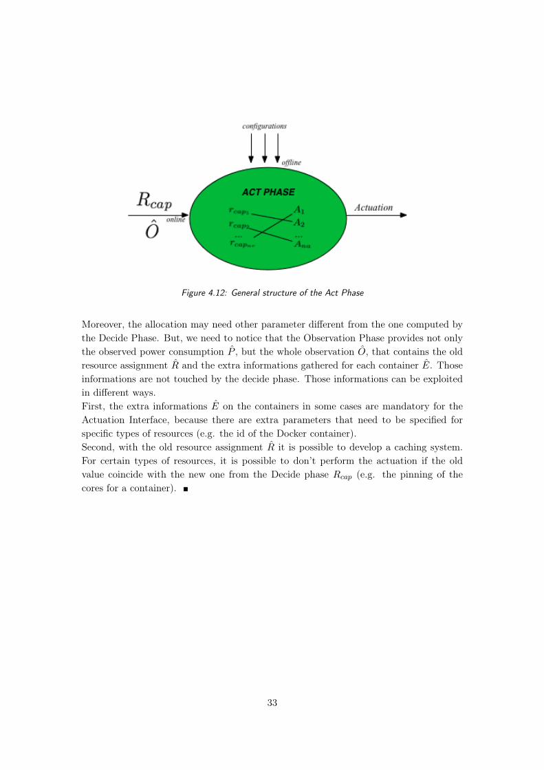
Figure 4.12: General structure of the Act Phase

Moreover, the allocation may need other parameter different from the one computed bythe Decide Phase. But, we need to notice that the Observation Phase provides not onlythe observed power consumption P , but the whole observation O, that contains the oldresource assignment R and the extra informations gathered for each container E. Thoseinformations are not touched by the decide phase. Those informations can be exploitedin different ways.First, the extra informations E on the containers in some cases are mandatory for theActuation Interface, because there are extra parameters that need to be specified forspecific types of resources (e.g. the id of the Docker container).Second, with the old resource assignment R it is possible to develop a caching system.For certain types of resources, it is possible to don’t perform the actuation if the oldvalue coincide with the new one from the Decide phase Rcap (e.g. the pinning of thecores for a container). �

33

Chapter 5

Implementation

In this chapter, we present the current implementation of DockerCap. In Section 5.1 wegive an overview on the properties of DockerCap and in Section 5.2 we give a detaileddescription of the architecture and on the functionalities of each component;

5.1 Implementation goals

DockerCap is a power capping orchestrator for Docker containers that manages resourcesto meet constraints on power consumption and to optimize the performances of thecontainers.In Chapter 4, we discussed about some properties that DockerCap needs to have. Inthe following sections, we explicit those properties and we highlight the implementationeffort that has been made to produce this orchestrator.Those properties are:

• ModularEvery component in DockerCap should be independent from the others. This allowus to develop and to plug-in different component without affecting the other partsof the system.

• ConfigurableEven if our system is modular, we also need each component of our system to beconfigurable, to adapt the specific need of the system.

• Provide precise cappingThis is an important property for a power capping system. We expect that theoscillations of the power consumption under strict power capping to be present,but we need to ensure that it is still limited.

• Provide performance guarantees for containersUnder the power constraints, we are interested in having guarantees on the per-formance of the running containers.

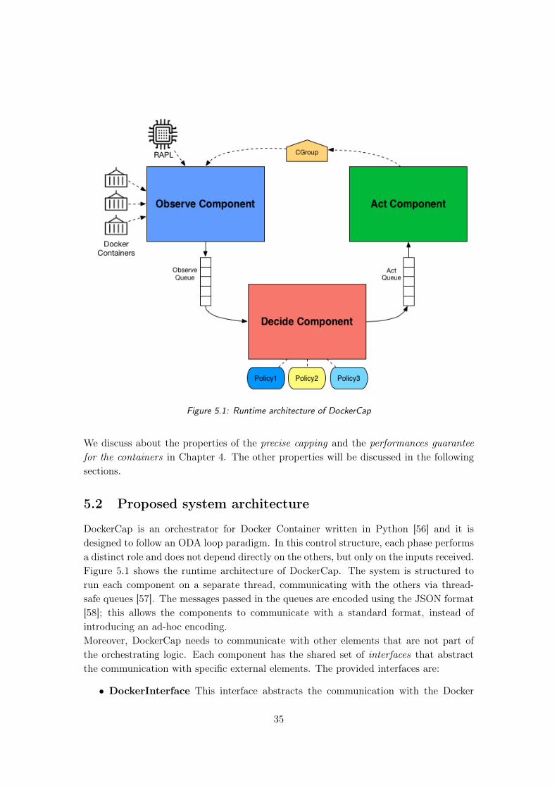
Figure 5.1: Runtime architecture of DockerCap

We discuss about the properties of the precise capping and the performances guaranteefor the containers in Chapter 4. The other properties will be discussed in the followingsections.

5.2 Proposed system architecture

DockerCap is an orchestrator for Docker Container written in Python [56] and it isdesigned to follow an ODA loop paradigm. In this control structure, each phase performsa distinct role and does not depend directly on the others, but only on the inputs received.Figure 5.1 shows the runtime architecture of DockerCap. The system is structured torun each component on a separate thread, communicating with the others via thread-safe queues [57]. The messages passed in the queues are encoded using the JSON format[58]; this allows the components to communicate with a standard format, instead ofintroducing an ad-hoc encoding.Moreover, DockerCap needs to communicate with other elements that are not part ofthe orchestrating logic. Each component has the shared set of interfaces that abstractthe communication with specific external elements. The provided interfaces are:

• DockerInterface This interface abstracts the communication with the Docker

35

Client [42]. It allows to gather information on the currently running containers(e.g. through the ps utility) and to perform actions that directly influence thecontainer, e.g. starting, stopping and killing a container.

• CGroupInterface This interface abstracts the access to the CGroup hierarchy [4].This is done mainly because the hierarchy may change with respect to the specificversion of the operating system or by how each CGroup is mounted. By adoptingthis interface, it is possible to get and set the values of: cpu_quota, cpu_period,memory_limits and cpuset (i.e. core pinning). To perform those actions, theinterface need to know informations such as the container id and how the hierarchyof the CGroups is structured (provided through configuration file).

• PerfInterface This interface abstracts the access of the perf tool to monitor hard-ware performance counters [59]. To do that, it hides the direct communication withthe tool and handle the parsing of the output provided by it. Currently, we adoptthe PerfInterface to read the value provided by the RAPL interface.

In the following subsection, we introduce other interfaces that were adopted only by spe-cific components of DockerCap. Each component exploits its own configuration and itsown submodules. The configuration file is stored as a XML file [60] in the folder of thecorresponding module. This configuration is then read by the module through a config-uration interface that abstracts the physical read of the file by providing the parametersin a data structure.

We developed three major modules that implement the three phases of the ODA loopdescribed in Chapter 4: the Observe Component, described in subsection 5.2.1, the De-cide Component, described in subsection 5.2.2, and the Act Component, described insubsection 5.2.3.

5.2.1 Observe Component

The Observe Component is the implementation of the Observe phase introduced in sec-tion 4.2. The goal of this component is to produce the observation O and to providethose data in the Observe Queue. The observation will be fetched from the queue by theDecide Component.To produce the observation O we need to compute the three basicelements that compose it: the observed power P , the current allocation of resources Rand the extra information on the containers E. The pseudocode of the Observe Com-ponent is described in Algorithm 1.

The observed power P is the aggregation of multiple power samples fetched through apower source. In general, the possible power source could be various, from external powermeters to internal sensors included in the hardware. Moreover, each power source needs

36

Algorithm 1 Observe Component pseudocode1: procedure Observe(ObserveQueue, powerSource, resourceSource)2: P ← powerSource.get_samples()3: R, E ← resourceSource.get_resources()4: O ← (P , R, E)

5: ObserveQueue.put(buildJSON(O))

6: return

to be treated differently from the others, especially in terms of sample time. For example,the RAPL interface [20] provides measurements in the order of ms; instead, the WattsUppower meter [61] provides power samples every second.That’s why we abstract the access on a specific power source through the interface Power-Source, that requires to specify the sample time and the how many power sample areneeded through configuration file of the Observe Component.The PowerSoure interface is implemented by the two types of power source supported byDockerCap: the RAPLPowerSource and the WattsUpPowerSource, that implement thecommunication with the RAPL interface and with the WattsUp Power meter interfacerespectively.On the one hand, the RAPLPowerSource gets the power sample from the RAPL interfaceby exploiting the Perf Linux tool. This tool provides access to the underlying perform-ance counters provided by the CPU and it is maintained by the Linux community. Tocommunicate with it, we developed the PerfInterface, that abstracts the specific com-munication with the tool. To read the power consumption of the CPU socket, RAPLdoesn’t read it directly from the hardware, but it implements internally a model of theHPC provided by the CPU [5]. It provides a minimum sampling time of 350ms [23].On the other hand, the WattsUpPowerSource gets the power sample from the attachedWattsUp power meter. The communication with the device is done by using the WattsUp[62] software interface. This interface communicate with the serial over USB and has asampling time of at least 1 second.The current allocation of resources and the extra information on the containers arefetched by a single source, the ResourceSource. To gather the extra informations, itexploits the DockerInterface to gather all the information needed about the running con-tainers. Then, through the CGroupInterface, it fetches the current resource allocation ofthe container. All the data gathered by the Observe Component through the interfacesare represented in Table 5.1.The objects powerSource and resourceSource are initialized when the DecideCompon-ent thread is launched. The choice of the specific PowerSource and ResourceSource ispossible by specifying it on the configuration file.

When we have all the information needed for the observation, we encode them in asingle JSON and then we send it in the ObserveQueue.

37

Table 5.1: Information gathered by the Observe Component

DockerInterface CGroupInterface PerfInterfacecontainer id cpu period observed power

image cpu quotacommand pinning

Listing 5.1: An example of a JSON produced by the Observe Component

{"timestamp": 1466462552,"power": 17.5,"resources": [{"id": "container1_ID","image": "contaner1","command": "container1 --type 2--input 37","cpu_period": 10000,"cpu_quota": 40000,"pinning": "0-4"

},{"id": "container2_ID","image": "container2"

...}]

}

An example of the produced JSON can be seen in Listing 5.1. Moreover, in the AppendixListing A.1 shows an example of the XML configuration file of the Observe Component.

5.2.2 Decide Component

The Decide Component is the implementation of the Decide phase described in section4.3. The goal of this component is to produce the new allocation of the resources forthe containers Rcap while guaranteeing the power cap P . This value is computed fromthe observation O, fetched from the ObserveQueue.The pseudocode that represents thewhole Decide Component is specified in Algorithm 2. It fetches from the ObserveQueuethe observation O, then it perform the decision through the chosen decider and finallyputs the new allocation of resources Rcap in the ActQueue.

38

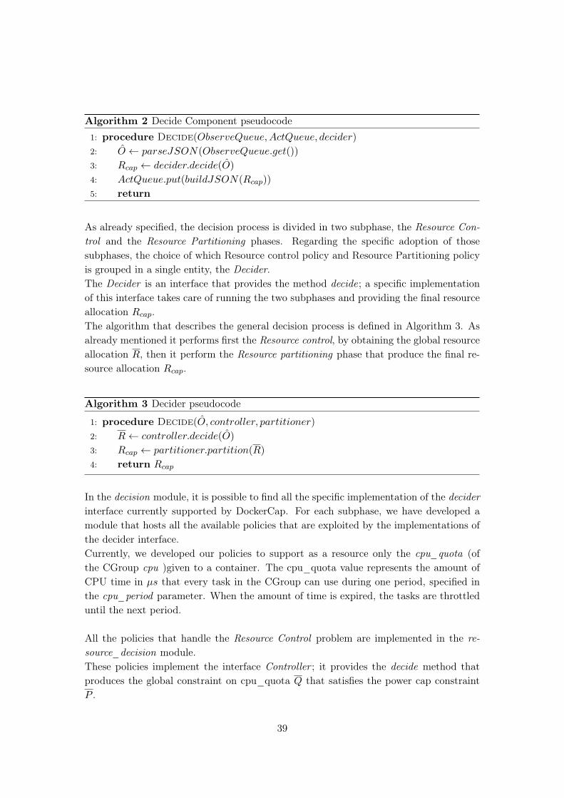
Algorithm 2 Decide Component pseudocode1: procedure Decide(ObserveQueue,ActQueue, decider)2: O ← parseJSON(ObserveQueue.get())

3: Rcap ← decider.decide(O)

4: ActQueue.put(buildJSON(Rcap))

5: return

As already specified, the decision process is divided in two subphase, the Resource Con-trol and the Resource Partitioning phases. Regarding the specific adoption of thosesubphases, the choice of which Resource control policy and Resource Partitioning policyis grouped in a single entity, the Decider.The Decider is an interface that provides the method decide; a specific implementationof this interface takes care of running the two subphases and providing the final resourceallocation Rcap.The algorithm that describes the general decision process is defined in Algorithm 3. Asalready mentioned it performs first the Resource control, by obtaining the global resourceallocation R, then it perform the Resource partitioning phase that produce the final re-source allocation Rcap.

Algorithm 3 Decider pseudocode

1: procedure Decide(O, controller, partitioner)2: R← controller.decide(O)

3: Rcap ← partitioner.partition(R)

4: return Rcap

In the decision module, it is possible to find all the specific implementation of the deciderinterface currently supported by DockerCap. For each subphase, we have developed amodule that hosts all the available policies that are exploited by the implementations ofthe decider interface.Currently, we developed our policies to support as a resource only the cpu_quota (ofthe CGroup cpu )given to a container. The cpu_quota value represents the amount ofCPU time in µs that every task in the CGroup can use during one period, specified inthe cpu_period parameter. When the amount of time is expired, the tasks are throttleduntil the next period.

All the policies that handle the Resource Control problem are implemented in the re-source_decision module.These policies implement the interface Controller ; it provides the decide method thatproduces the global constraint on cpu_quota Q that satisfies the power cap constraintP .

39

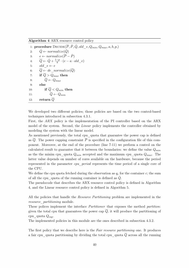
Algorithm 4 ARX resource control policy

1: procedure Decide(P , P , Q, old_e,Qmin, Qmax, a, b, p,)2: Q← normalize(Q)

3: e← normalize(P − P )

4: Q← Q+ 1−pb · (e− a · old_e)

5: old_e← e

6: Q← de_normalize(Q)

7: if Q > Qmax then8: Q← Qmax

9: else10: if Q < Qmin then11: Q← Qmin

12: return Q

We developed two different policies; those policies are based on the two control-basedtechniques introduced in subsection 4.3.1.First, the ARX policy is the implementation of the PI controller based on the ARXmodel of the system. Second, the Linear policy implements the controller obtained bymodeling the system with the linear model.As mentioned previously, the total cpu_quota that guarantee the power cap is definedas Q. The power capping constraint P is specified in the configuration file of this com-ponent. Moreover, at the end of the procedure (line 7-11) we perform a control on thecalculated result to guarantee that it between the boundaries: we define the value Qmin

as the the minim cpu_quota Qmin accepted and the maximum cpu_quota Qmax. Thelatter value depends on number of cores available on the hardware, because the periodrepresented in the parameter cpu_period represents the time period of a single core ofthe CPU.We define the cpu quota fetched during the observation as qc for the container c; the sumof all the cpu_quota of the running container is defined as Q.The pseudocode that describes the ARX resource control policy is defined in Algorithm4, and the Linear resource control policy is defined in Algorithm 5.

All the policies that handle the Resource Partitioning problem are implemented in theresource_partitioning module.These polices implement the interface Partitioner that exposes the method partition:given the total cpu that guarantees the power cap Q, it will produce the partitioning ofcpu_quota Qcap.The implemented policies in this module are the ones described in subsection 4.3.2.

The first policy that we describe here is the Fair resource partitioning one. It producesa fair cpu_quota partitioning by dividing the total cpu_quota Q across all the running

40

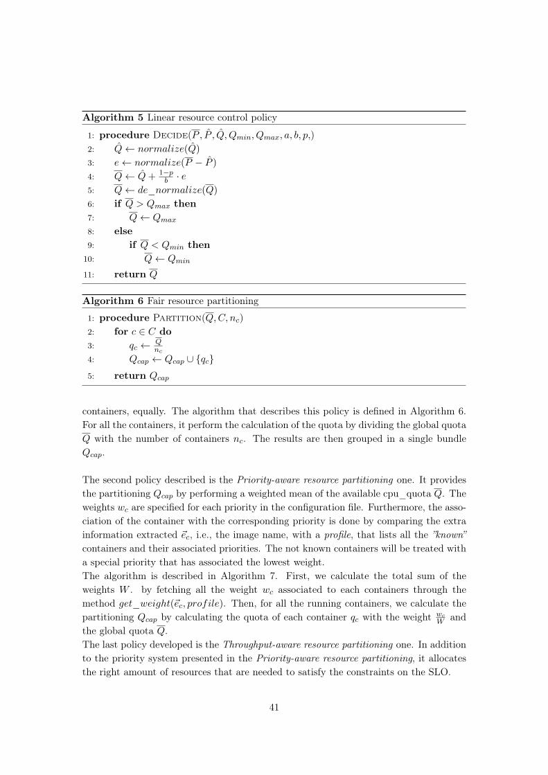
Algorithm 5 Linear resource control policy

1: procedure Decide(P , P , Q, Qmin, Qmax, a, b, p,)2: Q← normalize(Q)

3: e← normalize(P − P )

4: Q← Q+ 1−pb · e

5: Q← de_normalize(Q)

6: if Q > Qmax then7: Q← Qmax

8: else9: if Q < Qmin then

10: Q← Qmin

11: return Q

Algorithm 6 Fair resource partitioning

1: procedure Partition(Q,C, nc)2: for c ∈ C do3: qc ← Q

nc

4: Qcap ← Qcap ∪ {qc}5: return Qcap

containers, equally. The algorithm that describes this policy is defined in Algorithm 6.For all the containers, it perform the calculation of the quota by dividing the global quotaQ with the number of containers nc. The results are then grouped in a single bundleQcap.

The second policy described is the Priority-aware resource partitioning one. It providesthe partitioning Qcap by performing a weighted mean of the available cpu_quota Q. Theweights wc are specified for each priority in the configuration file. Furthermore, the asso-ciation of the container with the corresponding priority is done by comparing the extrainformation extracted ~ec, i.e., the image name, with a profile, that lists all the ”known”containers and their associated priorities. The not known containers will be treated witha special priority that has associated the lowest weight.The algorithm is described in Algorithm 7. First, we calculate the total sum of theweights W . by fetching all the weight wc associated to each containers through themethod get_weight(~ec, profile). Then, for all the running containers, we calculate thepartitioning Qcap by calculating the quota of each container qc with the weight wc

W andthe global quota Q.The last policy developed is the Throughput-aware resource partitioning one. In additionto the priority system presented in the Priority-aware resource partitioning, it allocatesthe right amount of resources that are needed to satisfy the constraints on the SLO.

41

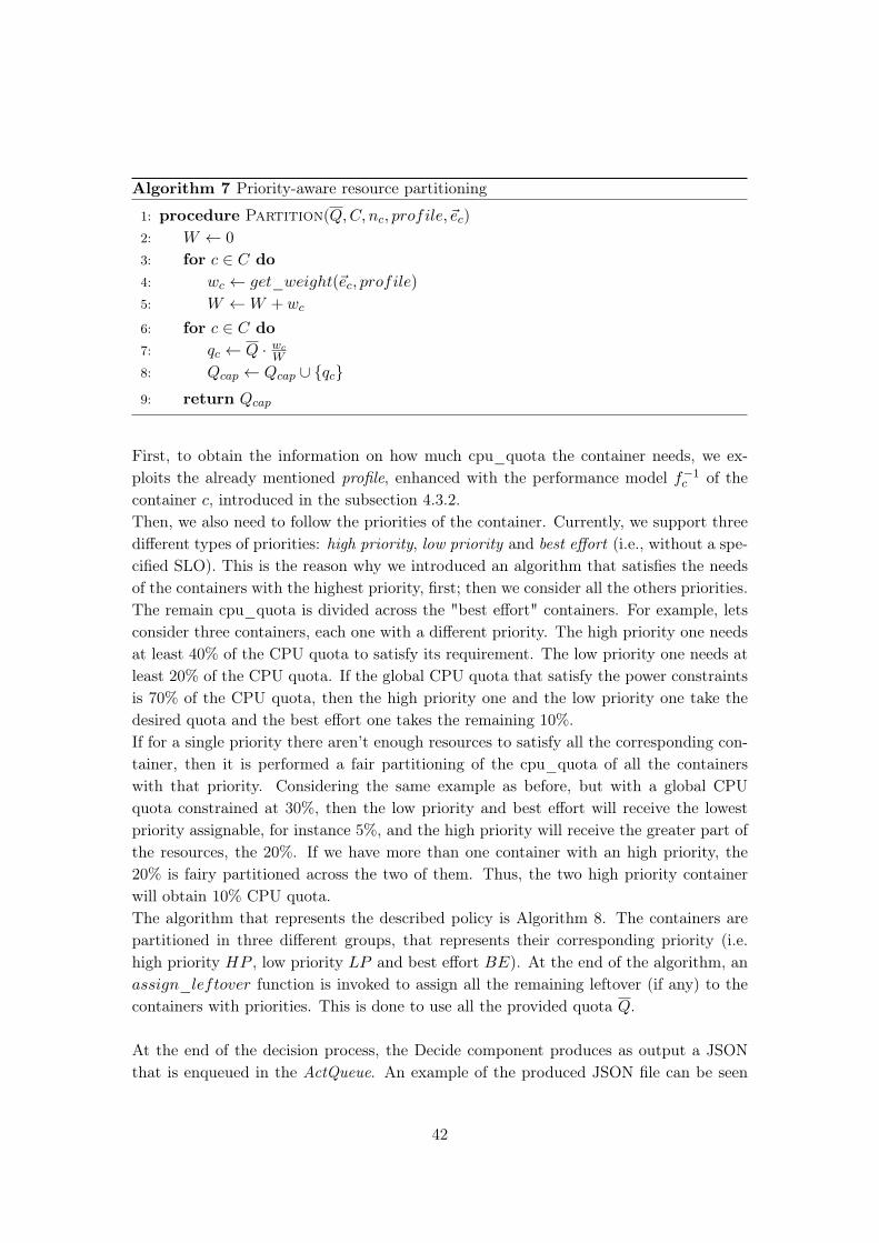
Algorithm 7 Priority-aware resource partitioning

1: procedure Partition(Q,C, nc, profile, ~ec)2: W ← 0

3: for c ∈ C do4: wc ← get_weight(~ec, profile)5: W ←W + wc

6: for c ∈ C do7: qc ← Q · wc

W

8: Qcap ← Qcap ∪ {qc}9: return Qcap

First, to obtain the information on how much cpu_quota the container needs, we ex-ploits the already mentioned profile, enhanced with the performance model f−1c of thecontainer c, introduced in the subsection 4.3.2.Then, we also need to follow the priorities of the container. Currently, we support threedifferent types of priorities: high priority, low priority and best effort (i.e., without a spe-cified SLO). This is the reason why we introduced an algorithm that satisfies the needsof the containers with the highest priority, first; then we consider all the others priorities.The remain cpu_quota is divided across the "best effort" containers. For example, letsconsider three containers, each one with a different priority. The high priority one needsat least 40% of the CPU quota to satisfy its requirement. The low priority one needs atleast 20% of the CPU quota. If the global CPU quota that satisfy the power constraintsis 70% of the CPU quota, then the high priority one and the low priority one take thedesired quota and the best effort one takes the remaining 10%.If for a single priority there aren’t enough resources to satisfy all the corresponding con-tainer, then it is performed a fair partitioning of the cpu_quota of all the containerswith that priority. Considering the same example as before, but with a global CPUquota constrained at 30%, then the low priority and best effort will receive the lowestpriority assignable, for instance 5%, and the high priority will receive the greater part ofthe resources, the 20%. If we have more than one container with an high priority, the20% is fairy partitioned across the two of them. Thus, the two high priority containerwill obtain 10% CPU quota.The algorithm that represents the described policy is Algorithm 8. The containers arepartitioned in three different groups, that represents their corresponding priority (i.e.high priority HP , low priority LP and best effort BE). At the end of the algorithm, anassign_leftover function is invoked to assign all the remaining leftover (if any) to thecontainers with priorities. This is done to use all the provided quota Q.

At the end of the decision process, the Decide component produces as output a JSONthat is enqueued in the ActQueue. An example of the produced JSON file can be seen

42

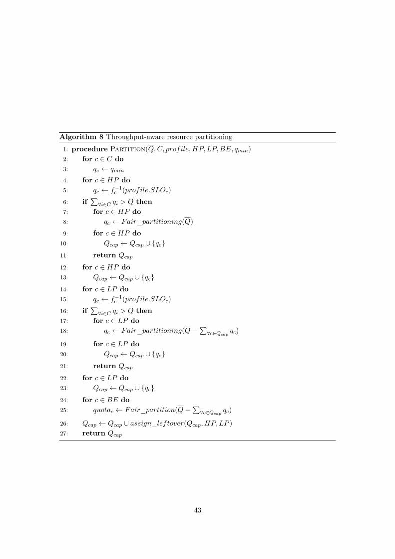
Algorithm 8 Throughput-aware resource partitioning

1: procedure Partition(Q,C, profile,HP,LP,BE, qmin)2: for c ∈ C do3: qc ← qmin

4: for c ∈ HP do5: qc ← f−1c (profile.SLOc)

6: if∑∀i∈C qi > Q then

7: for c ∈ HP do8: qc ← Fair_partitioning(Q)

9: for c ∈ HP do10: Qcap ← Qcap ∪ {qc}11: return Qcap

12: for c ∈ HP do13: Qcap ← Qcap ∪ {qc}14: for c ∈ LP do15: qc ← f−1c (profile.SLOc)

16: if∑∀i∈C qi > Q then

17: for c ∈ LP do18: qc ← Fair_partitioning(Q−

∑∀c∈Qcap

qc)

19: for c ∈ LP do20: Qcap ← Qcap ∪ {qc}21: return Qcap

22: for c ∈ LP do23: Qcap ← Qcap ∪ {qc}24: for c ∈ BE do25: quotac ← Fair_partition(Q−

∑∀c∈Qcap

qc)

26: Qcap ← Qcap ∪ assign_leftover(Qcap, HP,LP )

27: return Qcap

43

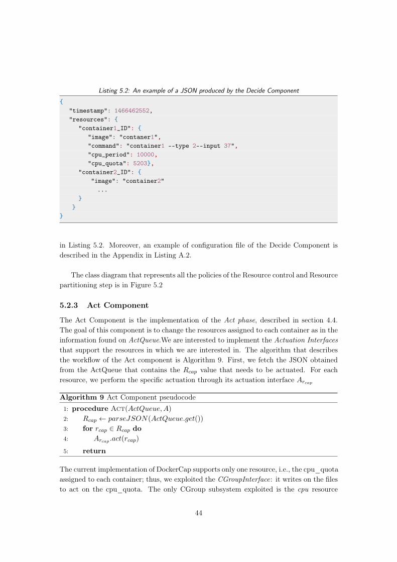
Listing 5.2: An example of a JSON produced by the Decide Component

{"timestamp": 1466462552,"resources": {

"container1_ID": {"image": "contaner1","command": "container1 --type 2--input 37","cpu_period": 10000,"cpu_quota": 5203},

"container2_ID": {"image": "container2"...

}}

}

in Listing 5.2. Moreover, an example of configuration file of the Decide Component isdescribed in the Appendix in Listing A.2.

The class diagram that represents all the policies of the Resource control and Resourcepartitioning step is in Figure 5.2

5.2.3 Act Component

The Act Component is the implementation of the Act phase, described in section 4.4.The goal of this component is to change the resources assigned to each container as in theinformation found on ActQueue.We are interested to implement the Actuation Interfacesthat support the resources in which we are interested in. The algorithm that describesthe workflow of the Act component is Algorithm 9. First, we fetch the JSON obtainedfrom the ActQueue that contains the Rcap value that needs to be actuated. For eachresource, we perform the specific actuation through its actuation interface Arcap

Algorithm 9 Act Component pseudocode1: procedure Act(ActQueue,A)2: Rcap ← parseJSON(ActQueue.get())

3: for rcap ∈ Rcap do4: Arcap .act(rcap)

5: return

The current implementation of DockerCap supports only one resource, i.e., the cpu_quotaassigned to each container; thus, we exploited the CGroupInterface: it writes on the filesto act on the cpu_quota. The only CGroup subsystem exploited is the cpu resource

44

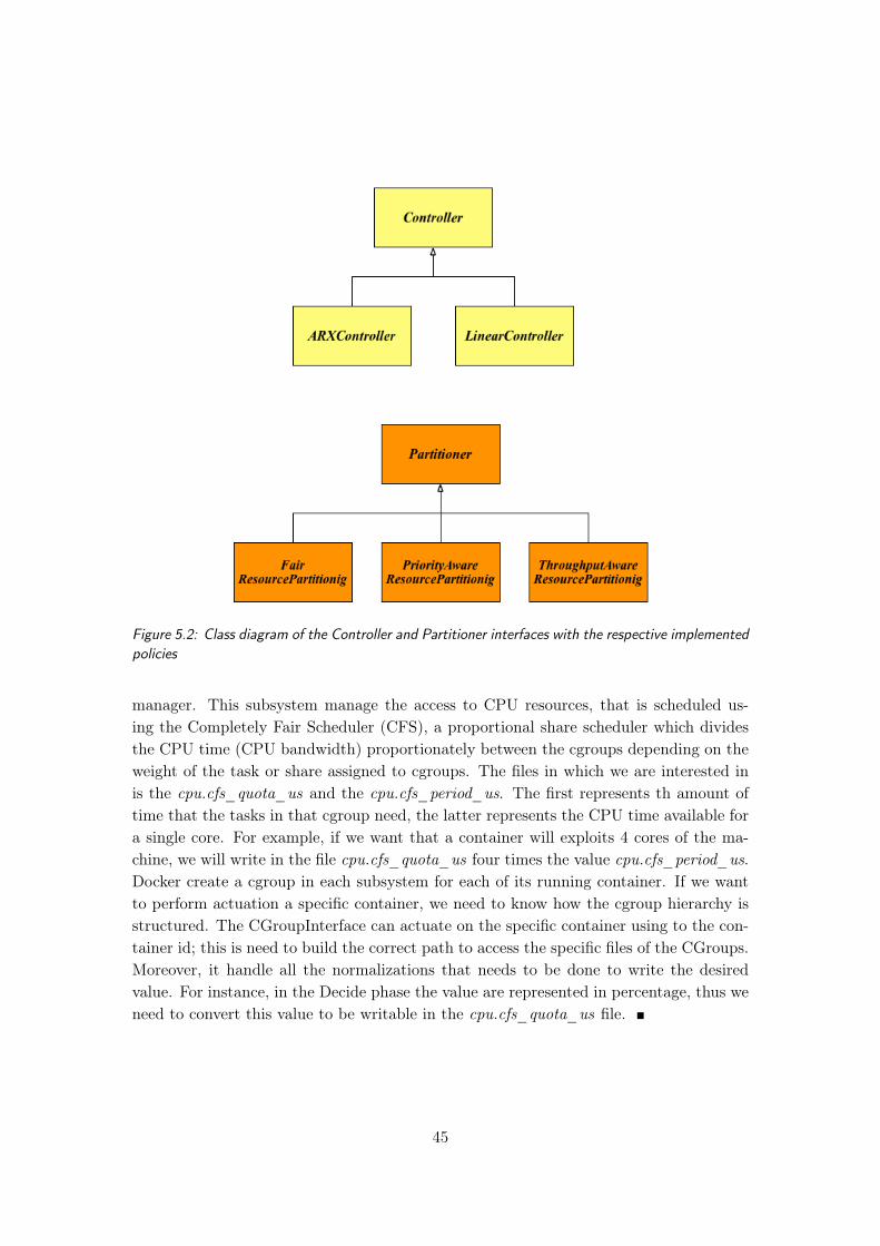
Figure 5.2: Class diagram of the Controller and Partitioner interfaces with the respective implementedpolicies

manager. This subsystem manage the access to CPU resources, that is scheduled us-ing the Completely Fair Scheduler (CFS), a proportional share scheduler which dividesthe CPU time (CPU bandwidth) proportionately between the cgroups depending on theweight of the task or share assigned to cgroups. The files in which we are interested inis the cpu.cfs_quota_us and the cpu.cfs_period_us. The first represents th amount oftime that the tasks in that cgroup need, the latter represents the CPU time available fora single core. For example, if we want that a container will exploits 4 cores of the ma-chine, we will write in the file cpu.cfs_quota_us four times the value cpu.cfs_period_us.Docker create a cgroup in each subsystem for each of its running container. If we wantto perform actuation a specific container, we need to know how the cgroup hierarchy isstructured. The CGroupInterface can actuate on the specific container using to the con-tainer id; this is need to build the correct path to access the specific files of the CGroups.Moreover, it handle all the normalizations that needs to be done to write the desiredvalue. For instance, in the Decide phase the value are represented in percentage, thus weneed to convert this value to be writable in the cpu.cfs_quota_us file. �

45

Chapter 6

Experimental results

In this chapter, we discuss the results obtained during the evaluation of DockerCap.As introduced in the previous chapters, DockerCap is a power capping orchestrator thatprovides control over the performances of the running containers. The proposed approachis compared with the state of the art power capping solution RAPL [20], an hardwareinterface provided by Intel in the processors since Sandy Bridge [5]. The proposed tech-niques and RAPL are evaluated with respect to two different metrics:

• Precision: how much the power consumption of the machine is close to the desiredpower cap;

• Performance: what are the performance of the running containers with each specificpower capping technique.

The chapter is organized as follows: in section 6.1 we define the experimental setupadopted during all our experiments; in section 6.2 we show the results in terms of precisionand in section 6.3 we show the results in terms of performances.

6.1 Experimental Setup

In this section, we give a description of the environment in which we developed and eval-uated DockerCap. Considering that we exploit Docker as container engine, our system isdeveloped to operate in a Linux environment, with a kernel that supports Linux ControlGroups [4] with CONFIG_CFS_BANDWIDTH set to "y" in the Kernel configurationto permit the CFS scheduler to limit the bandwidth rates for tasks running in the groups.

The adopted processor is an Intel Xeon E5-1410 [63] that supports the RAPL [20]interface, Turbo Boost [64] and Simultaneous Multithreading (SMT) [65] technology.During our experiments, we disable both Turbo Boost and SMT to remove all the non-linear behaviors of the power consumption that may occur during the execution of thebenchmarks. Currently, DockerCap supports two types of power source. To allow theObserve Component to exploit a given power source, it is necessary to deploy DockerCapin contexts that support those sources:

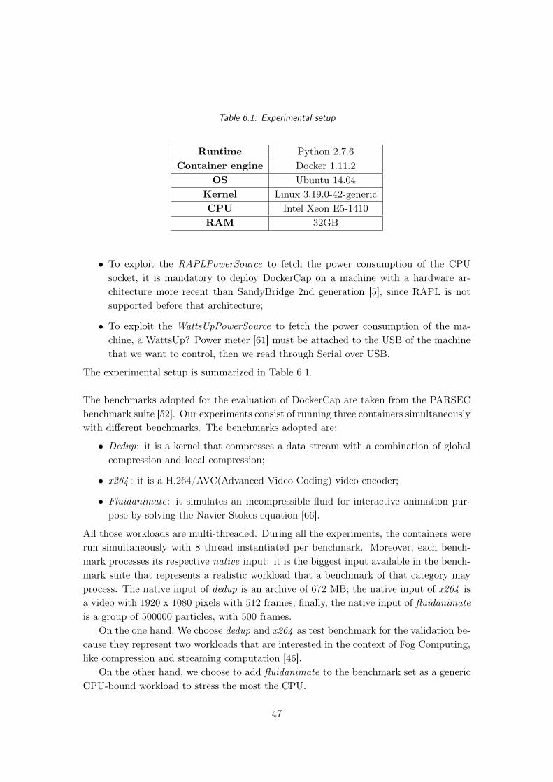
Table 6.1: Experimental setup

Runtime Python 2.7.6Container engine Docker 1.11.2

OS Ubuntu 14.04Kernel Linux 3.19.0-42-genericCPU Intel Xeon E5-1410RAM 32GB

• To exploit the RAPLPowerSource to fetch the power consumption of the CPUsocket, it is mandatory to deploy DockerCap on a machine with a hardware ar-chitecture more recent than SandyBridge 2nd generation [5], since RAPL is notsupported before that architecture;

• To exploit the WattsUpPowerSource to fetch the power consumption of the ma-chine, a WattsUp? Power meter [61] must be attached to the USB of the machinethat we want to control, then we read through Serial over USB.

The experimental setup is summarized in Table 6.1.

The benchmarks adopted for the evaluation of DockerCap are taken from the PARSECbenchmark suite [52]. Our experiments consist of running three containers simultaneouslywith different benchmarks. The benchmarks adopted are:

• Dedup: it is a kernel that compresses a data stream with a combination of globalcompression and local compression;

• x264 : it is a H.264/AVC(Advanced Video Coding) video encoder;

• Fluidanimate: it simulates an incompressible fluid for interactive animation pur-pose by solving the Navier-Stokes equation [66].

All those workloads are multi-threaded. During all the experiments, the containers wererun simultaneously with 8 thread instantiated per benchmark. Moreover, each bench-mark processes its respective native input: it is the biggest input available in the bench-mark suite that represents a realistic workload that a benchmark of that category mayprocess. The native input of dedup is an archive of 672 MB; the native input of x264 isa video with 1920 x 1080 pixels with 512 frames; finally, the native input of fluidanimateis a group of 500000 particles, with 500 frames.

On the one hand, We choose dedup and x264 as test benchmark for the validation be-cause they represent two workloads that are interested in the context of Fog Computing,like compression and streaming computation [46].

On the other hand, we choose to add fluidanimate to the benchmark set as a genericCPU-bound workload to stress the most the CPU.

47

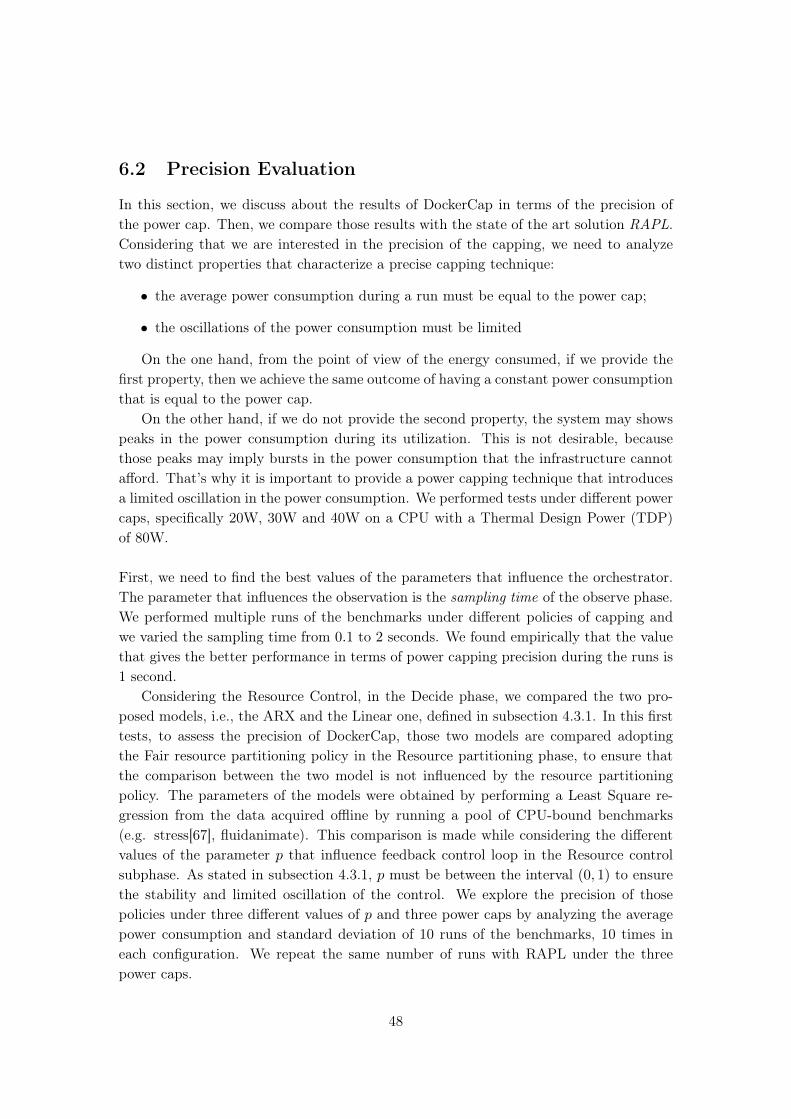
6.2 Precision Evaluation

In this section, we discuss about the results of DockerCap in terms of the precision ofthe power cap. Then, we compare those results with the state of the art solution RAPL.Considering that we are interested in the precision of the capping, we need to analyzetwo distinct properties that characterize a precise capping technique:

• the average power consumption during a run must be equal to the power cap;

• the oscillations of the power consumption must be limited

On the one hand, from the point of view of the energy consumed, if we provide thefirst property, then we achieve the same outcome of having a constant power consumptionthat is equal to the power cap.

On the other hand, if we do not provide the second property, the system may showspeaks in the power consumption during its utilization. This is not desirable, becausethose peaks may imply bursts in the power consumption that the infrastructure cannotafford. That’s why it is important to provide a power capping technique that introducesa limited oscillation in the power consumption. We performed tests under different powercaps, specifically 20W, 30W and 40W on a CPU with a Thermal Design Power (TDP)of 80W.

First, we need to find the best values of the parameters that influence the orchestrator.The parameter that influences the observation is the sampling time of the observe phase.We performed multiple runs of the benchmarks under different policies of capping andwe varied the sampling time from 0.1 to 2 seconds. We found empirically that the valuethat gives the better performance in terms of power capping precision during the runs is1 second.

Considering the Resource Control, in the Decide phase, we compared the two pro-posed models, i.e., the ARX and the Linear one, defined in subsection 4.3.1. In this firsttests, to assess the precision of DockerCap, those two models are compared adoptingthe Fair resource partitioning policy in the Resource partitioning phase, to ensure thatthe comparison between the two model is not influenced by the resource partitioningpolicy. The parameters of the models were obtained by performing a Least Square re-gression from the data acquired offline by running a pool of CPU-bound benchmarks(e.g. stress[67], fluidanimate). This comparison is made while considering the differentvalues of the parameter p that influence feedback control loop in the Resource controlsubphase. As stated in subsection 4.3.1, p must be between the interval (0, 1) to ensurethe stability and limited oscillation of the control. We explore the precision of thosepolicies under three different values of p and three power caps by analyzing the averagepower consumption and standard deviation of 10 runs of the benchmarks, 10 times ineach configuration. We repeat the same number of runs with RAPL under the threepower caps.

48

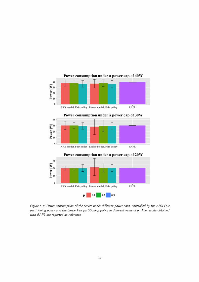
Figure 6.1: Power consumption of the server under different power caps, controlled by the ARX Fairpartitioning policy and the Linear Fair partitioning policy in different value of p. The results obtainedwith RAPL are reported as reference

49

Figure 6.2: Power consumption of the server under different power caps, controlled by the threeproposed Partitioning policy with the ARX model used in the controller

Figure 6.1 shows that on average the power consumption of the machine is equal tothe power cap in the two stricter power cap (i.e. 20W and 30W), while under 40W themean power consumption is lower than the cap.

Moreover, in terms of standard deviation, the ARX Fair partitioning outperform theLinear one in all the considered values of p and power caps. This highlights that, even ifthe considerations on the linear power-resources model are legit, a linear model with theparameter learned offline is not precise enough to perform better than an ARX offlinemodel: as a consequence, in the next evaluations we consider the ARX controller as thereference solution.

In all the proposed configurations, the ARX Fair partitioning model performs betterwith p equals to 0.5: again, this value is then used during all our experimental evaluationsthat follows in Section 6.3.

As expected, RAPL outperforms our solution in terms of precision: this is reasonable,as our solution is a software-based power capping and with resource management aloneit is not possible to achieve the same precision of RAPL, that has a direct control overthe hardware frequency and voltage of the processors. Instead, DockerCap in the bestconfiguration shows an average power consumption that is close to the power cap with astandard deviation of ≈ 4.2W in all the partitioning policies.

Then, we analyzed the power consumption of all the proposed policies under the ARXcontroller, since it is the one that performs better in terms of oscillations. Figure 6.2 shows

50

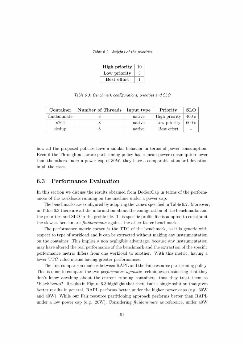
Table 6.2: Weights of the priorities

High priority 10Low priority 3Best effort 1

Table 6.3: Benchmark configurations, priorities and SLO

Container Number of Threads Input type Priority SLOfluidanimate 8 native High priority 400 s

x264 8 native Low priority 600 sdedup 8 native Best effort -

how all the proposed policies have a similar behavior in terms of power consumption.Even if the Throughput-aware partitioning policy has a mean power consumption lowerthan the others under a power cap of 30W, they have a comparable standard deviationin all the cases.

6.3 Performance Evaluation

In this section we discuss the results obtained from DockerCap in terms of the perform-ances of the workloads running on the machine under a power cap.

The benchmarks are configured by adopting the values specified in Table 6.2. Moreover,in Table 6.3 there are all the information about the configuration of the benchmarks andthe priorities and SLO in the profile file. This specific profile file is adopted to constraintthe slowest benchmark fluidanimate against the other faster benchmarks.

The performance metric chosen is the TTC of the benchmark, as it is generic withrespect to type of workload and it can be extracted without making any instrumentationon the container. This implies a non negligible advantage, because any instrumentationmay have altered the real performance of the benchmark and the extraction of the specificperformance metric differs from one workload to another. With this metric, having alower TTC value means having greater performances.

The first comparison made is between RAPL and the Fair resource partitioning policy.This is done to compare the two performance-agnostic techniques, considering that theydon’t know anything about the current running containers, thus they treat them as"black boxes". Results in Figure 6.3 highlight that there isn’t a single solution that givesbetter results in general. RAPL performs better under the higher power caps (e.g. 30Wand 40W). While our Fair resource partitioning approach performs better than RAPLunder a low power cap (e.g. 20W). Considering fluidanimate as reference, under 40W

51

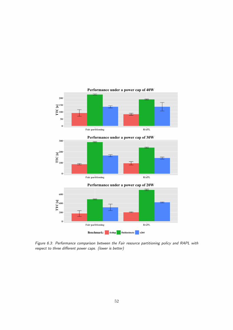
Figure 6.3: Performance comparison between the Fair resource partitioning policy and RAPL withrespect to three different power caps. (lower is better)

52

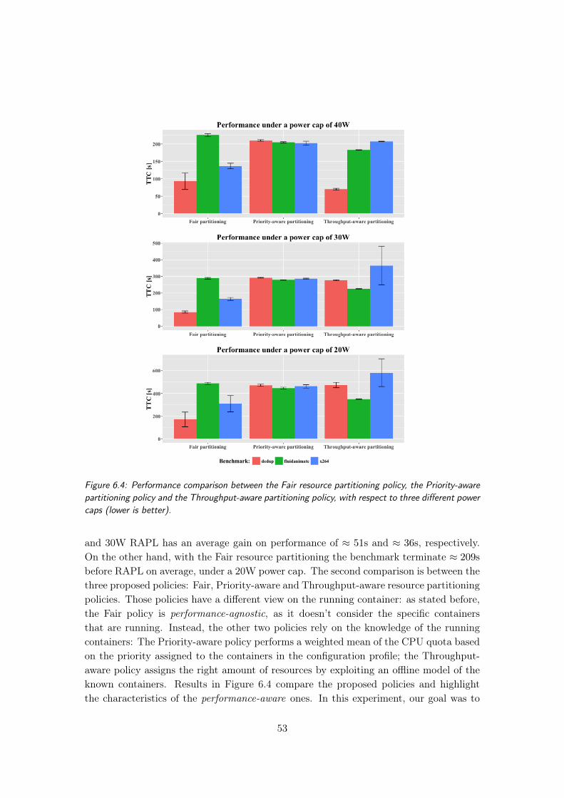
Figure 6.4: Performance comparison between the Fair resource partitioning policy, the Priority-awarepartitioning policy and the Throughput-aware partitioning policy, with respect to three different powercaps (lower is better).

and 30W RAPL has an average gain on performance of ≈ 51s and ≈ 36s, respectively.On the other hand, with the Fair resource partitioning the benchmark terminate ≈ 209sbefore RAPL on average, under a 20W power cap. The second comparison is between thethree proposed policies: Fair, Priority-aware and Throughput-aware resource partitioningpolicies. Those policies have a different view on the running container: as stated before,the Fair policy is performance-agnostic, as it doesn’t consider the specific containersthat are running. Instead, the other two policies rely on the knowledge of the runningcontainers: The Priority-aware policy performs a weighted mean of the CPU quota basedon the priority assigned to the containers in the configuration profile; the Throughput-aware policy assigns the right amount of resources by exploiting an offline model of theknown containers. Results in Figure 6.4 compare the proposed policies and highlightthe characteristics of the performance-aware ones. In this experiment, our goal was to

53

increase the performance of fluidanimate, the slowest benchmark under the performance-agnostic policies.

The Priority-aware partitioning policy tunes the resources following the prioritiesgiven to the container. By choosing an appropriate assignment of weights, it is possible toobtain the same TTC for all the containers. In this case, the performance of fluidanimateare improved w.r.t. the Fair partitioning.

The Throughput-aware partitioning allocates the right amount of resources that needsto satisfy the SLO by following their priorities. We gave a high priority with a SLO of400s to the benchmark fluidanimate. Under high power cap (e.g. 40W and 30W), inall the policies (including RAPL), fluidanimate satisfies its performance constraints forall the policies, thanks to the less strict constraints on the resources. On the contrary,under a low power cap (e.g. 20W) the Throughput-aware partitioning policy is the onlyone able to satisfy the performance constraints, because it always assigns the resourcesthat fluidanimate needs at the expense of the other running containers. Thus, it is theonly technique able to satisfy the SLA of the container. �

54

Chapter 7

Conclusions and Future work

Power management is a key aspect that needs to be considered in nowadays technologies.With the great diffusion of IoT technologies, the need of storing and processing data leadsto an increasing adoption of Cloud in the IoT environment. In this context, the Cloudwas obliged to extends its computation near to the physical devices, mostly to scaleproperly and to provide specific functionalities needed by specific IoT applications. Thishas led the introduction of a new paradigm: Fog Computing. With this technology,the computation is taken near the physical device through specific computational units,defined as fog nodes. Those nodes cannot dispose of a great amount of energy, becausethey are usually deployed in a domestic environment or they are battery-powered. Thus,to provide an higher availability for fog nodes, we need to adopt power managementtechniques to limit the consumption of a single node still guaranteeing its constraints onperformances. Moreover, in this context there is the need of moving the computationbetween the cloud and the fog.

In this thesis work we proposed DockerCap: a performances-aware orchestrator forDocker containers that manages their assigned resource at runtime to meet constraints onpower consumption and the performance requirements of different tenants. We developDockerCap by following the ODA control loop, a well known approach of control systemsand a policy-based system to tune the performance of the containers.

In the Observe phase, we gather the information that represents the current state ofthe system that hosts DockerCap: the power consumption of the machine, the currentallocation of the resources, specifically the CPU quota, and extra information about therunning containers.

In the Decide phase, we focus on computing a new allocation of resources that willtake the system to satisfy its constraints, both in terms of power consumption and per-formances. To better tackle these requirements, we divide the decision problem in twosubphases. In the first subphase, called Resource control, we decide the global allocationof resources that the containers will exploit. In this subphase, the focus is satisfying theconstraint on the power consumption of the machine. We develop a controller that, giventhe current power consumption and an offline model of the machine, it will provide theglobal allocation of resources that needs to be assigned to stay under the power cap. Thesecond subphase, called Resource Partitioning, focuses on partitioning the whole amount

of resources, provided by the previous subphase, to tune the performances of the runningcontainers. In this subphase, we develop a policy-based system and we propose threepolicies that handle the resources to reach for different purposes. The first policy, theFair resource partitioning, simply splits the CPU quota in equals parts for all the run-ning containers. The second policy, the Priority-aware resource partitioning, performs aweighted mean of the CPU quota based on the priority assigned to each containers. Thethird and last proposed policy is the Throughput-aware partitioning policy; by followingthe priority of the containers, it allocates the right amount of resources needed to satisfythe SLO of a specific container. The information about the priorities and the amount ofresources required to satisfy the constraints on performances are given through a profilefile. By performing the two subphases sequentially, we obtain the amount of CPU Quotathat needs to be assigned for each container.

In the Act phase, we perform the actual allocation of the resources by exploiting theLinux Control Groups, all of this based on the allocation computed in the previous step.

In order to evaluate our proposed solution, we compare all our proposed policies withthe state of the art power capping solution RAPL, both in terms of precision and perform-ances. In the precision evaluation, we analyze how the controlled system behaves whenDockerCap enforces a power cap, expressed in terms of the mean power consumption.Instead, in the performance evaluation we analyze the performance of each benchmarkunder a power cap with respect to its requirements. From the results obtained, we seethat RAPL provides better precision in terms of power capping, thanks to its capabilityto operate directly on the voltage and frequency of the processors and its fast reactiontime. On the other hand, our proposed policies provide a better alternative to RAPLin terms of performances, in a multi-tenant scenario. The Fair resource partitioningprovides better performances under a lower power cap, and comparable performancesunder higher power caps. The Priority-aware resource partitioning policy can uniformlydistribute the resources such that the TTC of the containers is the same. Moreover, theresults obtained with the Throughput-aware policy shows that it is possible to guaranteethe SLO of specific workloads, in contrast with the other techniques, while still guaran-teeing the power constraints.

Future work The most incumbent work that can improve DockerCap is related tothe precision of the power capping. An interesting option that needs to be explored is theadoption of the MARC framework [68] during the Resource control phase. This couldlead to an improvement in the precision of the model of the system S adopted in thefeedback control, thus providing a more precise capping.

Another option could be to add in the control loop the possibility of learning the modelof the system online, through RLS or a Kalman filter [53]. With an online model, it ispossible to adapt the control with respect to the containers that are currently running.

Unfortunately, a software-based power capping technique is not enough to provide a

56

power capping as precise as an hardware-based one, like RAPL. Regarding this issue, it isnecessary to integrate RAPL in the DockerCap methodology to exploit the advantages ofboth the techniques: a fast and precise power capping and a fine-grained control over theresources of the containers to satisfy the constraints on the performances of the tenants.

Another important aspect that needs to be extended is the observation of the perform-ances of the running containers. Currently, DockerCap exploits a resource-performancemodel of the container that is computed offline; this it is not always feasible in a Cloudenvironment, where you host workloads that are not known a priori. In this context,there is the need of obtaining those informations at runtime, by extracting metrics aboutthe current computation. Those metrics can provide information on the right allocationof resources that satisfy the performance requirements. Moreover, it is not easy to obtaina performance metric at runtime from the container, because a general workload doesnot provide such data. We recommend to explore the possibility of adopting the hard-ware performance counters as a metric to gather useful information about the runningcontainers. �

57

Bibliography

[1] Flavio Bonomi, Rodolfo Milito, Jiang Zhu and Sateesh Addepalli. Fog computingand its role in the internet of things. In Proceedings of the first edition of the mccworkshop on mobile cloud computing. ACM, 2012, pages 13–16.

[2] Qi Zhang, Lu Cheng and Raouf Boutaba. Cloud computing: state-of-the-art andresearch challenges. Journal of internet services and applications, 1(1):7–18, 2010.

[3] Toni Mastelic, Ariel Oleksiak, Holger Claussen, Ivona Brandic, Jean-Marc Piersonand Athanasios V Vasilakos. Cloud computing: survey on energy efficiency. Acmcomputing surveys (csur), 47(2):33, 2015.

[4] Linux cgroups. July 2016. url: https://www.kernel.org/doc/Documentation/cgroup-v1/cgroups.txt.

[5] Efraim Rotem, Alon Naveh, Avinash Ananthakrishnan, Doron Rajwan and EliezerWeissmann. Power-management architecture of the intel microarchitecture code-named sandy bridge. Ieee micro, (2):20–27, 2012.

[6] Franck L Lewis et al. Wireless sensor networks. Smart environments: technologies,protocols, and applications:11–46, 2004.

[7] Luigi Atzori, Antonio Iera and Giacomo Morabito. The internet of things: a survey.Computer networks, 54(15):2787–2805, 2010.

[8] Ala Al-Fuqaha, Mohsen Guizani, Mehdi Mohammadi, Mohammed Aledhari andMoussa Ayyash. Internet of things: a survey on enabling technologies, protocols,and applications. Ieee communications surveys & tutorials, 17(4):2347–2376, 2015.

[9] Enerdata. Global energy statistical yearbook 2014. 2014. url: http://yearbook.enerdata.net/ (visited on 2016).

[10] U.S. EIA. International energy outlook 2016 with projections to 2040. technicalreport. 2016. url: http://www.eia.gov/forecasts/ieo/pdf/0484(2016).pdf(visited on 2016).

[11] European Communities European Commission. Energy efficiency plan 2011. tech-nical report. 2011. url: http://ec.europa.eu/clima/policies/strategies/2050/docs/efficiency_plan_en.pdf (visited on 2016).

[12] Hadi Esmaeilzadeh, Emily Blem, Renee St Amant, Karthikeyan Sankaralingamand Doug Burger. Dark silicon and the end of multicore scaling. In Computerarchitecture (isca), 2011 38th annual international symposium on. IEEE, 2011,pages 365–376.

58

[13] Ganesh Venkatesh, Jack Sampson, Nathan Goulding, Saturnino Garcia, VladyslavBryksin, Jose Lugo-Martinez, Steven Swanson and Michael Bedford Taylor. Conser-vation cores: reducing the energy of mature computations. In Acm sigarch computerarchitecture news. Volume 38. (1). ACM, 2010, pages 205–218.

[14] Robert R Schaller. Moore’s law: past, present and future. Spectrum, ieee, 34(6):52–59, 1997.

[15] Michael B Taylor. Is dark silicon useful?: harnessing the four horsemen of the com-ing dark silicon apocalypse. In Proceedings of the 49th annual design automationconference. ACM, 2012, pages 1131–1136.

[16] Jean-Marc Pierson. Large-scale distributed systems and energy efficiency: a holisticview. John Wiley & Sons, 2015.

[17] Andreas Berl, Erol Gelenbe, Marco Di Girolamo, Giovanni Giuliani, Hermann DeMeer, Minh Quan Dang and Kostas Pentikousis. Energy-efficient cloud computing.The computer journal, 53(7):1045–1051, 2010.

[18] Xi Fang, Satyajayant Misra, Guoliang Xue and Dejun Yang. Smart gridâăťthenew and improved power grid: a survey. Ieee communications surveys & tutorials,14(4):944–980, 2012.

[19] Mazeiar Salehie and Ladan Tahvildari. Self-adaptive software: landscape and re-search challenges. Acm transactions on autonomous and adaptive systems (taas),4(2):14, 2009.

[20] Howard David, Eugene Gorbatov, Ulf R Hanebutte, Rahul Khanna and ChristianLe. Rapl: memory power estimation and capping. In Low-power electronics anddesign (islped), 2010 acm/ieee international symposium on. IEEE, 2010, pages 189–194.

[21] Ramya Raghavendra, Parthasarathy Ranganathan, Vanish Talwar, Zhikui Wangand Xiaoyun Zhu. No power struggles: coordinated multi-level power managementfor the data center. In Acm sigarch computer architecture news. Volume 36. (1).ACM, 2008, pages 48–59.

[22] Xiaorui Wang, Ming Chen and Xing Fu. Mimo power control for high-densityservers in an enclosure. Parallel and distributed systems, ieee transactions on,21(10):1412–1426, 2010.

[23] Huazhe Zhang and Henry Hoffmann. Maximizing performance under a power cap:a comparison of hardware, software, and hybrid techniques. In International con-ference on architectural support for programming languages and operating systems(asplos), 2016.

[24] Qingyuan Deng, David Meisner, Arup Bhattacharjee, Thomas F Wenisch and Ri-cardo Bianchini. Coscale: coordinating cpu and memory system dvfs in server sys-tems. In Microarchitecture (micro), 2012 45th annual ieee/acm international sym-posium on. IEEE, 2012, pages 143–154.

59

[25] Qingyuan Deng, David Meisner, Abhishek Bhattacharjee, Thomas F Wenisch andRicardo Bianchini. Multiscale: memory system dvfs with multiple memory control-lers. In Proceedings of the 2012 acm/ieee international symposium on low powerelectronics and design. ACM, 2012, pages 297–302.

[26] Ryan Cochran, Can Hankendi, Ayse K Coskun and Sherief Reda. Pack & cap: ad-aptive dvfs and thread packing under power caps. In Proceedings of the 44th annualieee/acm international symposium on microarchitecture. ACM, 2011, pages 175–185.

[27] Krishna K Rangan, Gu-Yeon Wei and David Brooks. Thread motion: fine-grainedpower management for multi-core systems. In Acm sigarch computer architecturenews. Volume 37. (3). ACM, 2009, pages 302–313.

[28] Jian Chen and Lizy Kurian John. Predictive coordination of multiple on-chip re-sources for chip multiprocessors. In Proceedings of the international conference onsupercomputing. ACM, 2011, pages 192–201.

[29] Henry Hoffmann and Martina Maggio. Pcp: a generalized approach to optimiz-ing performance under power constraints through resource management. In 11thinternational conference on autonomic computing (icac 14), 2014, pages 241–247.

[30] Martina Maggio, Henry Hoffmann, Marco D Santambrogio, Anant Agarwal andAlberto Leva. Power optimization in embedded systems via feedback control ofresource allocation. Control systems technology, ieee transactions on, 21(1):239–246, 2013.

[31] David Meisner, Christopher M Sadler, Luiz André Barroso, Wolf-Dietrich Weberand Thomas F Wenisch. Power management of online data-intensive services. InComputer architecture (isca), 2011 38th annual international symposium on. IEEE,2011, pages 319–330.

[32] Ripal Nathuji and Karsten Schwan. Virtualpower: coordinated power manage-ment in virtualized enterprise systems. In Acm sigops operating systems review.Volume 41. (6). ACM, 2007, pages 265–278.

[33] Vlasia Anagnostopoulou, Susmit Biswas, Heba Saadeldeen, Ricardo Bianchini, TaoYang, Diana Franklin and Frederic T Chong. Power-aware resource allocationfor cpu-and memory-intense internet services. In, Energy efficient data centers,pages 69–80. Springer, 2012.

[34] Wes Felter, Karthick Rajamani, Tom Keller and Cosmin Rusu. A performance-conserving approach for reducing peak power consumption in server systems. InProceedings of the 19th annual international conference on supercomputing. ACM,2005, pages 293–302.

[35] Xiaodong Li, Ritu Gupta, Sarita V Adve and Yuanyuan Zhou. Cross-componentenergy management: joint adaptation of processor and memory. Acm transactionson architecture and code optimization (taco), 4(3):14, 2007.

60

[36] Jonathan A Winter, David H Albonesi and Christine A Shoemaker. Scalable threadscheduling and global power management for heterogeneous many-core architec-tures. In Proceedings of the 19th international conference on parallel architecturesand compilation techniques. ACM, 2010, pages 29–40.

[37] Xiaodong Li, Zhenmin Li, Francis David, Pin Zhou, Yuanyuan Zhou, Sarita Adveand Sanjeev Kumar. Performance directed energy management for main memoryand disks. Acm sigplan notices, 39(11):271–283, 2004.

[38] Keith Adams and Ole Agesen. A comparison of software and hardware techniquesfor x86 virtualization. Acm sigplan notices, 41(11):2–13, 2006.

[39] Paul Barham, Boris Dragovic, Keir Fraser, Steven Hand, Tim Harris, Alex Ho, RolfNeugebauer, Ian Pratt and AndrewWarfield. Xen and the art of virtualization. Acmsigops operating systems review, 37(5):164–177, 2003.

[40] Avi Kivity, Yaniv Kamay, Dor Laor, Uri Lublin and Anthony Liguori. Kvm: thelinux virtual machine monitor. In Proceedings of the linux symposium. Volume 1,2007, pages 225–230.

[41] Fabrice Bellard. Qemu, a fast and portable dynamic translator. In Usenix annualtechnical conference, freenix track, 2005, pages 41–46.

[42] Docker. Docker - build, ship, and run any app, anywhere. 2013. url: https://www.docker.com (visited on 2016).

[43] Linux kernel. July 2016. url: https://www.kernel.org.

[44] Linux namespaces. July 2016. url: http://man7.org/linux/man-pages/man7/namespaces.7.html.

[45] Dave Evans. The internet of things: how the next evolution of the internet is chan-ging everything. Cisco white paper, 1:1–11, 2011.

[46] Jiang Zhu, Douglas S Chan, Mythili Suryanarayana Prabhu, Prem Natarajan, HaoHu and Flavio Bonomi. Improving web sites performance using edge servers in fogcomputing architecture. In Service oriented system engineering (sose), 2013 ieee7th international symposium on. IEEE, 2013, pages 320–323.

[47] Ben Zhang, Nitesh Mor, John Kolb, Douglas S Chan, Ken Lutz, Eric Allman,John Wawrzynek, Edward Lee and John Kubiatowicz. The cloud is not enough:saving iot from the cloud. In 7th usenix workshop on hot topics in cloud computing(hotcloud 15), 2015.

[48] Joseph L Hellerstein, Yixin Diao, Sujay Parekh and Dawn M Tilbury. Feedbackcontrol of computing systems. John Wiley & Sons, 2004.

[49] Davide B Bartolini, Filippo Sironi, Donatella Sciuto and Marco D Santambrogio.Automated fine-grained cpu provisioning for virtual machines. Acm transactionson architecture and code optimization (taco), 11(3):27, 2014.

61

[50] Filippo Sironi, Martina Maggio, Riccardo Cattaneo, Giovanni F Del Nero, Dona-tella Sciuto and Marco D Santambrogio. Thermos: system support for dynamicthermal management of chip multi-processors. In Parallel architectures and com-pilation techniques (pact), 2013 22nd international conference on. IEEE, 2013,pages 41–50.

[51] Oxford English Dictionary. Oxford: oxford university press. 1989. url: http://www.oxforddictionaries.com (visited on 2016).

[52] Christian Bienia, Sanjeev Kumar, Jaswinder Pal Singh and Kai Li. The parsecbenchmark suite: characterization and architectural implications. In Proceedingsof the 17th international conference on parallel architectures and compilation tech-niques. ACM, 2008, pages 72–81.

[53] Rudolph Emil Kalman. A new approach to linear filtering and prediction problems.Journal of basic engineering, 82(1):35–45, 1960.

[54] Pierre Simon marquis de Laplace. Théorie analytique des probabilités. V. Courcier,1820.

[55] Norman R Draper and Harry Smith. Applied regression analysis. John Wiley &Sons, 2014.

[56] Python. Python - work quickly and integrate systems more effectively. 1991. url:https://www.python.org (visited on 2016).

[57] Python. Queue - python module that implements multi-producer, multi-consumersqueue. url: https://docs.python.org/2/library/queue.html (visited on2016).

[58] JSON. Json - a lightweight data-interchange format. url: http://www.json.org(visited on 2016).

[59] Liunx. Perf - monitoring performance counters on linux. 2009. url: https://perf.wiki.kernel.org/index.php/Main_Page (visited on 2016).

[60] W3. Xml - simple and very flexible text format. 2007. url: http://www.w3.org/XML/ (visited on 2016).

[61] Communicationsprotocol090824, 2015. url: https://goo.gl/ZKzctJ (visited on2016).

[62] pyrovski. Wattsup - a program for interfacing with the watts up? power meter.2012. url: https://github.com/pyrovski/watts-up (visited on 2016).

[63] Intel. Intel xeon processor e5-1410 specifications. 2012. url: http://ark.intel.com/products/67417/Intel-Xeon-Processor-E5-1410-10M-Cache-2_8-GHz(visited on 2016).

[64] Intel. Intel turbo boost technology 2.0. 2012. url: http://www.intel.com/content/www/us/en/architecture-and-technology/turbo-boost/turbo-boost-technology.html (visited on 2016).

62

[65] Dean M Tullsen, Susan J Eggers and Henry M Levy. Simultaneous multithread-ing: maximizing on-chip parallelism. In Acm sigarch computer architecture news.Volume 23. (2). ACM, 1995, pages 392–403.

[66] D. Pnueli and C. Gutfinger. Fluid mechanics. Cambridge University Press, 1992.

[67] Liunx. Stress - tool to impose load on and stress test systems. url: http://linux.die.net/man/1/stress (visited on 2016).

[68] Andrea Corna and Andrea Damiani. A scalable framework for resource consump-tion modelling: the marc approach. Master’s thesis. Politecnico di Milano, 2016.

63

Appendix A

DockerCap configuration

This appendix describes the configuration files adopted in DockerCap.

The first file is the configuration file of the Observe Component. It is divided in threedifferent secitons:

• default: contains all the parameters needed by the general Observe phase.

• watts-up: contains all the parameters needed by the WattsUpPowerSource

• rapl: contains all the parameters needed by the RAPLPowerSource

The WattsUpPowerSource needs to know the serial ID of the power meter attached bythe USB and the path to the executable that permits the power readings.The RAPLPowerSource, needs only the sample time (in ms) to perform the powersamplings. An example of the configuration is represented in Listing A.1.

The second file is the configuration file of the Decide Component. It is divided in multiplesections, as follows:

• default: contains all the parameters needed by the general Decide phase.

• arx: contains all the parameters needed by the ARX Resource control

• linear: contains all the parameters needed by the Linear Resource Control

• partitioner: contains all the parameters needed by the Partitioning policies

Regarding the default section, It is possible to specify the Decider chosen in the de-cision process by writing its label in the controller parameter.The variable power_initand power_cap represent the init value that will be passed to the Decider and the powercap P that the resource control phase must guarantee. The path in which will be writtenthe log files is described in the output value. Last, we have quota_min as the minimumvalue of global CPU quota that can be assigned.Instead, in the arx and linear sections, they contains all the parameter that are specificfor the controller, like the weights of the model a and b, the pole p and the parameter

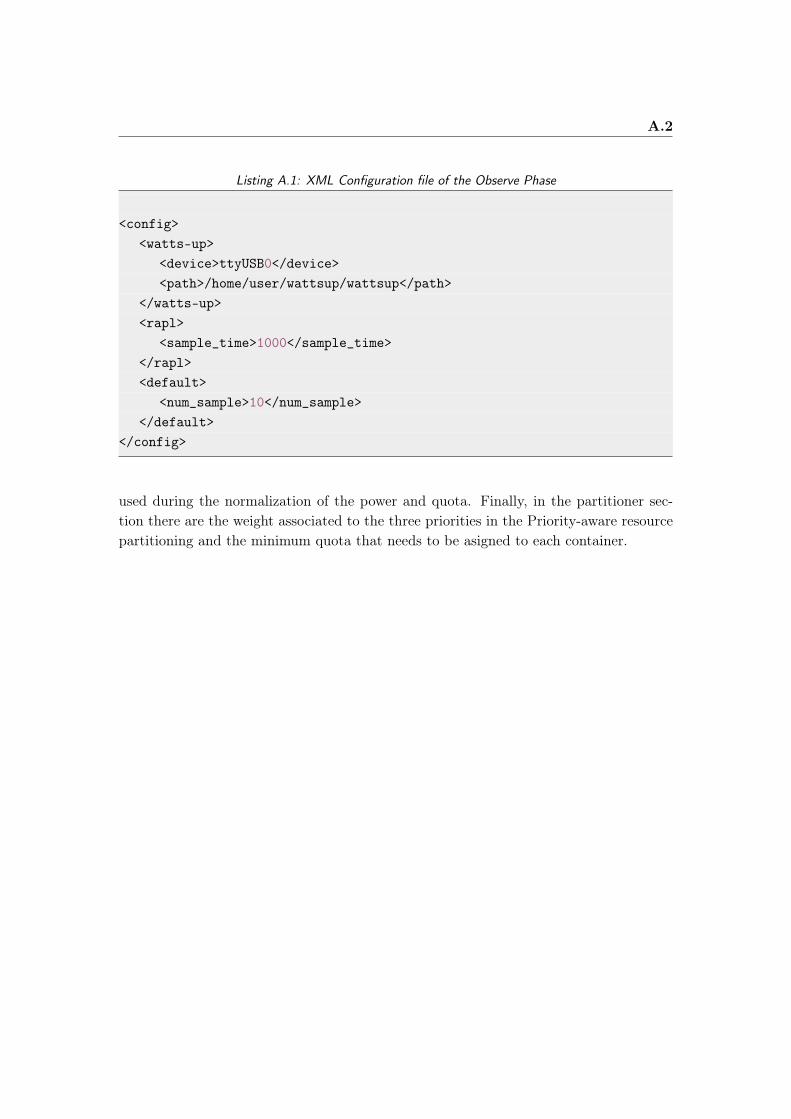
A.2

Listing A.1: XML Configuration file of the Observe Phase

<config><watts-up>

<device>ttyUSB0</device><path>/home/user/wattsup/wattsup</path>

</watts-up><rapl>

<sample_time>1000</sample_time></rapl><default>

<num_sample>10</num_sample></default>

</config>

used during the normalization of the power and quota. Finally, in the partitioner sec-tion there are the weight associated to the three priorities in the Priority-aware resourcepartitioning and the minimum quota that needs to be asigned to each container.

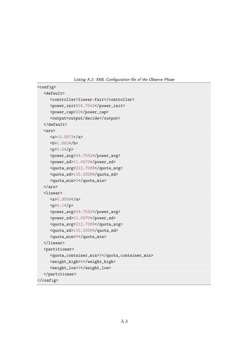
Listing A.2: XML Configuration file of the Observe Phase

<config><default>

<controller>linear-fair</controller><power_init>24.7542</power_init><power_cap>20</power_cap><output>output/decide</output>

</default><arx>

<a>-0.5673</a><b>1.662</b><p>0.5</p><power_avg>24.7542</power_avg><power_sd>11.0470</power_sd><quota_avg>212.7088</quota_avg><quota_sd>115.3326</quota_sd><quota_min>5</quota_min>

</arx><linear>

<a>0.9558</a><p>0.1</p><power_avg>24.7542</power_avg><power_sd>11.0470</power_sd><quota_avg>212.7088</quota_avg><quota_sd>115.3326</quota_sd><quota_min>5</quota_min>

</linear><partitioner>

<quota_container_min>5</quota_container_min><weight_high>5</weight_high><weight_low>3</weight_low>

</partitioner></config>

A.3