Embed Size (px)
Citation preview
Université de Carthage
THÈSE
Préparée à
L’École Supérieure des Communications de Tunis
En vue d’obtenir le Diplôme de
DOCTEUR
En
Technologies de l’Information et de la Communication
Par
Nazih HAJRI
Thème
Performance Analysis of Mobile-to-Mobile
Communications over Hoyt Fading Channels
Soutenue à SUP’COM le 11 Mars 2011 devant le jury d’examen composé de : Président M. Ammar BOUALLEGUE Professeur à L’ENIT Rapporteurs M. Mohamed-Slim ALOUINI Professeur à KAUST M. Nourredine HAMDI Maître de Conférences à l’INSAT Examinateur M. Sofiène CHERIF Maître de Conférences à SUP’COM Directeur de Thèse M. Néji YOUSSEF Professeur à SUP’COM
Universite de Carthage
THESE
Preparee a
L’Ecole Superieure des Communications de Tunis
En vue d’obtenir le Diplome de
DOCTEUR
En
Technologies de l’Information et de la Communication
Par
Nazih HAJRI
Theme
Performance Analysis of Mobile-to-Mobile
Communications over Hoyt Fading Channels
Soutenue a SUP’COM le 11 Mars 2011 devant le jury d’examen compose de :
President M. Ammar Bouallegue Professeur a L’ENIT
Rapporteurs M. Mohamed-Slim Alouini Professeur a KAUST
M. Nourredine Hamdi Maıtre de Conferences a l’INSAT
Examinateur M. Sofiene Cherif Maıtre de Conferences a SUP’COM
Directeur de These M. Neji Youssef Professeur a SUP’COM

Acknowledgments
Praise be to God, the most gracious and the most merciful. Without his blessing and guidance
my accomplishments would never been possible.
I’am grateful to many people who helped me during the course of this work. First, I would
like to thank my advisor and director Prof. Neji Youssef for his excellent guidance and support
during my thesis work. He has taught me a lot; including to be a persevering researcher as well
as being creative, thoughtful, and being crafty in presenting ideas and writing papers. He is
also a perfect gentleman who is always nice, polite, and considerate. He was a genuine model
forme from whom I have learned so much from him and I owe a lot to his patience.
I owe my deepest gratitude to Prof. Mohammed Slim-Alouinie and Dr. Nourredine Hamdi
for the time and effort that they invested in the proofreading of this dissertation. Their remarks
and comments have contributed to improve the quality of the text. I also want to thank the
chairman Prof. Ammar Bouallegue and the jury member Dr. Sofiene Cherif for investing their
precious time and experience in this PhD.
Then, my appreciation goes to Prof. Matthias Patzold at the Faculty of Engineering and
Science at the University of Adger, for his pleasant and efficient scientific collaboration which
resulted in several joint publications.
I would like also to present my warm thanks to all the academic and the supporting staff at
the Higher School of Communications of Tunis (Sup’com) for their kind assistance and generous
professional support during my graduate studies.
I warmly thank my colleague Soumeyya Ben Aıcha from Institut Superieur d’Informatique
et de Mathematiques at Monastir for revising the English of my manuscript.
Also, I want to thank several of my best friends. In particular, my special thanks go to
Baddredine Bouzouita, Sami Brahim, Mohamed Mghaiegh, and Mohamed Ali Smeda for their
continuous support and love.
. . .
And at the end, I would like to give my deepest thanks to my fiancee Soumeya Bouchareb,
my parents Abdelsalem and Latifa, my sisters Nadia and Imen, and my brothers Amine and
Riadth for their unconditional love, support, and their belief in my potential. Certainly, this
thesis would have not been possible without their support. I am and I will be indebted to them
for their warm love and their absolute confidence in me.
i
Abstract
Mobile-to-mobile (M2M) communications, where both the transmitter and receiver are in motion, find
many applications in ad-hoc wireless networks, intelligent transportation systems, and relay-based cel-
lular networks. For both an effective M2M communication systems design and a related performance
analysis, the appropriate propagation characteristics have to be taken into account. In this respect, the
investigation of the error rate performance of the digital transmission has been widely studied for the case
of M2M Rayleigh, Rice, and Nakagami-m fading channels. Recently, and besides these most frequently
used channels, the Hoyt fading is a widely accepted statistical model to characterize the short-term
multipath effects, where the fading conditions are more severe than those of the Rayleigh case. Given
the importance of the Hoyt fading channel, it is of a great interest, therefore, to study and analyze its
impact on the performance of the wireless M2M communication systems. In this thesis, we contribute
to the topic of the performance analysis of various digital transmission schemes over M2M Hoyt fading
channels. In this context, our work can be divided into two essential parts. In the first one, we present
a study on the performance analysis of the main digital angular modulation schemes under single Hoyt
fading channels, taking into account the Doppler spread effects caused by the motion of the mobile
transmitter and receiver, i.e, the case of a single Hoyt fading with a double-Doppler or M2M single Hoyt
fading channels. In this framework, closed-form expressions for the bit error probability (BEP) perfor-
mance of the differential phase-shift keying (PSK) modulation and frequency-shift keying (FSK) with
limiter-discriminator integrator and differential detection schemes have been addressed under M2M Hoyt
fading channels. In the second part, we introduce the double Hoyt fading model, which can be useful in
the modeling of M2M fading channels, where the multipath propagation conditions are worse than those
described by the double Rayleigh fading. This model assumes that the overall complex channel gain,
between a mobile transmitter and a receiver, is modeled as the product of the gains of two statistically
independent single Hoyt channels. By considering this M2M multipath fading distribution, the first and
the second order statistics of the double Hoyt fading channels are first derived. As it is known, the
second order statistics in terms of the level-crossing rate (or equivalently the frequency of outages) and
average duration of fades (or equivalently the average outage duration) represent important commonly
performance measures of wireless communication systems that are used to reflect the correlation prop-
erties of the fading channels and provide a dynamic representation of the system outage performance.
Then, expressions for the main first and second order statistics of the corresponding channel capacity
process are also investigated. Finally, the BEP of the digital modulated signals that are transmitted over
slow and frequency flat double Hoyt fading channels is studied. In this case, a generic expression for the
average BEP of coherent binary PSK, quadrature PSK, FSK, minimum-shift keying, and amplitude-shift
keying modulation schemes is derived.
Index Terms— Mobile-to-mobile communications, bit error probability performance, Hoyt
fading channels, mobile-to-mobile Hoyt fading channels, double Hoyt fading channels, probability of
outage, average outage duration, frequency of outages, digital modulation schemes.
ii
Preface
The work presented in this thesis has been published and presented in variety national and
international conferences. Specifically, the thesis work has resulted in the following publications.
International Conferences
• N. Hajri, N. Youssef, F. Choubani, and T. Kawabata. BER performance of M2M communi-
cations over double Hoyt fading channels. Proc. 21th Annual IEEE International Symposium
on Personal, Indoor and Mobile Radio Communications 2010 (PIMRC’10), Istanbul, Turkey,
pp. 1–5, Sept. 2010.
• N. Hajri, N. Youssef, and M. Patzold. On the statistical properties of the capacity of double
Hoyt fading channels. Proc. 11th IEEE International Workshop on Signal Processing Advances
for Wireless Communications 2010 (SPAWC’10), Marrakech, Morocco, pp. 1–5, Jun. 2010.
• N. Hajri, N. Youssef, and M. Patzold. A study on the statistical properties of double
Hoyt fading channels. Proc. 6th IEEE International Symposium on Wireless Communication
Systems 2009 (ISWCS’09), Siena, Italy, pp. 201–205, Sept. 2009.
• N. Hajri, N. Youssef, and Matthias Patzold. Performance analysis of binary DPSK modula-
tion schemes over Hoyt fading channels. Proc. 6th IEEE International Symposium on Wireless
Communication Systems 2009 (ISWCS’09), Siena, Italy, pp. 609–613, Sept. 2009.
• N. Hajri and N. Youssef. On the performance analysis of FSK using differential detection
over Hoyt fading channels. Proc. 2nd IEEE International Conference on Signals, Circuits&
Systems (SCS’08), Hammamet, Tunisia, pp. 1–5, Nov. 2008.
• N. Hajri and N. Youssef. Performance analysis of FSK modulation with limiter-discriminator-
integrator detection over Hoyt fading channels. Proc. International Conference on Wireless
Information Networks and Systems (WINSYS’08), Porto-Portugal, pp. 177–181, Jul. 2008.
• N. Hajri and N. Youssef. Bit error probability of narrow-band digital FM with limiter-
discriminator-integrator detection in Hoyt mobile radio fading channels. Proc. 18th Annual
IEEE International Symposium on Personal, Indoor and Mobile Radio Communications 2007
(PIMRC’07), Greece, Athens, pp. 1–5, Sept. 2007.
iii

Preface
National Conferences
• N. Hajri and N. Youssef. On the distribution of the phase difference between two Hoyt
processes perturbed by Gaussian noise. Proc. Kantaoui Forum 9, Tunisia-Japan Symposium
on Society, Science & Technology 2008 (KF9–TJASSST’08), Kantaoui, Sousse, Tunisia, pp.
1–3, Nov. 2008.
iv

Nomenclature
List of Acronyms
AAF Amplify and Forward
ABER Average Bit Error Rate
ACF Autocorrelation Function
ADF Average Duration of Fades
AMPS Advance Mobile Phone Service
AoA Angle of Arrival
AoD Angle of Departure
AoF Amount of Fading
ASEP Average Symbol Error Probability
ASK Amplitude Shift Keying
AWGN Additive White Gaussian Noise
BEP Bit Error Probability
BPSK Binary Phase-Shift-Keying
BS Base Station
CDF Cumulative Distribution Function
CDMA Code Division Multiple Access
CPM Continuous Phase Modulation
DPSK Differential Phase-Shift-Keying
DS Direct Sequence
DSRC Dedicated Short Range Communications
EGC Equal Gain Combining
ETACS European Total Access Communication System
F2M Fixed-to-Mobile
FM Frequency Modulation
FSK Frequency-Shift-Keying
GMSK Gaussian Minimum Shift Keying
IF Intermediate Frequency
IHVS Intelligent Highway Vehicular Systems
v

Nomenclature
iid independent and identically distributed
ISI InterSymbol Interference
LCR Level Crossing Rate
LD Limiter-Discriminator
LDI Limiter-Discriminator-Integrator
LOS Line-Of-Sight
LPNM Lp-Norm Method
M-DPSK M -ary Differential Phase-Shift Keying
M-QAM M -ary Quadrature Amplitude Modulation
M2M Mobile-to-Mobile
MEDS Method of Exact Doppler Spread
MIMO Multiple-Input Multiple-Output
MRC Maximum Ratio Combining
MSR Mobile Station Receiver
MST Mobile Station Transmitter
MSEM Mean Square Error Method
MSK Minimum Shift Keying
PDF Probability Density Function
PSD Power Spectrum Density
PSK Phase-Shift-Keying
QPSK Quadrature Phase-Shift Keying
RS Relay Station
SIMO Single-Input Multiple-Output
SISO Single-Input Single-Output
SNR Signal-to-Noise Ratio
List of Symbols
αR,n The AoA of the nth path measured with respect to the velocity vector−→VR
αT,n The AoD of the nth path measured with respect to the velocity vector−→VT
α The ratio between the maximum Doppler frequencies fR,max and fT,max
γ,γs The average signal-to-noise ratio
βij The negative curvature of the autocorrelation function Γµijµij (t) (i, j = 1, 2) at τ = 0
vi
Nomenclature
Γµiµi(τ) The curvature of the autocorrelation function Γµijµij (t) (i, j = 1, 2)
∆η The phase noise difference due to additive Gaussian noise
∆φ The data phase difference
∆ϑ The phase difference introduced by the Hoyt fading channel
∆Ω The phase difference between two Hoyt faded signals perturbed by Gaussian noise
∆Ψ The overall phase difference at the output of a LDI circuit
ψ(t) The derivative of the overall phase ψ(t) with respect to the time t
Ξ(t) The time derivative process of Ξ(t)
Ξ2(t) The time derivative of the process Ξ2(t)
R(t) The time derivative process of R(t)
η(t) The phase caused by additive Gaussian noise
Γµiµi(τ) The temporal autocorrelation function of the process µi(t) (i = 1, 2)
Γnn(τ) The temporal autocorrelation function of the process ni(t) (i = 1, 2)
γ(t),γs(t) The instaneous signal-to-noise ratio
Γµijµij (τ) The temporal autocorrelation function of the process µij (i = 1, 2)
Γgsigsi (τ) The temporal autocorrelation function of the process gsi(t) (i = 1, 2)
Λ The ratio between the variances σ211 and σ2n
µij(t) Zero-mean Gaussian process (i, j = 1, 2)
µ1(t) The Hoyt channel gain process
Ω(t) The phase caused by the Hoyt fading plus additive Gaussian noise
N The average number of FM clicks
P b The average BEP performance in double Hoyt fading channels
−→VR The velocity vector due to the motion of the receiver
−→VT The velocity vector due to the motion of the transmitter
φ(t) The filtered signal phase after FM modulation
ψ(t) The overall phase at the output of the limiter circuit
ρµ11+n The normalized ACF of the process (µ11(t) + n1(t))
ρτ1 The normalized ACF of the process µ1i(t) (i = 1, 2)
Σ The covariance matrix of the vector process (x1, y1, x2, y2)t
σ2 The mean power of the Hoyt fading process R(t)
Σ−1 The inverse matrix of the covariance matrix Σ
vii
Nomenclature
σ2n The average power of the additive Gaussian noise n(t)
σ2DiThe variance of the single Rayleigh fading process RDi(t) (i = 1, 2)
σ2i0 The reduced variance of the process µ1i(t) (i = 1, 2)
σ2ij The variance of the process µij(t) (i, j = 1, 2)
σ2s1 The variance of the process gsi(t) (i = 1, 2)
Θ(t) The phase process of the double Hoyt fading channel
θ(t) The FSK data phase
θn The random phase
θi,n The phase of the deterministic process µ1i(t) (i = 1, 2)
θij,n The phase of the deterministic process µij(t) (i, j = 1, 2)
θR,k The random phase around the mobile station receiver
θT,k The random phase around the mobile station transmitter
Υ(t) The complex double Hoyt channel gain process
ϑ(t), ϑi(t) The single Hoyt channel phase process (i = 1, 2)
µij(t) The deterministic process corresponding to the process µij(t) (i, j = 1, 2)
Ξ(t) The double Hoyt fading process
Ξ2(t) The double Hoyt channel power gain
ζi, ξi The noise component defined relatively to the coordinate system that rotate with φ1
(i = 1, 2)
a(t) The filtered carrier amplitude
Ak The random amplitude around the mobile station transmitter
B The equivalent noise bandwidth
b(t) The binary data sequence
Bn The random amplitude around the mobile station receiver
BT The bandwidth-time product coefficient
C(t) The normalized time varying capacity process of double Hoyt fading channels
cn The amplitude of the nth propagation path
ci,n The gains of the deterministic process µ1i(t) (i = 1, 2)
cij,n The gains of the deterministic process µij(t) (i, j = 1, 2)
ckn The joint amplitude caused by the interaction of the transmitter and receiver scat-terers
e(t) The Hoyt faded sinusoid signals perturbed by Gaussian noise
viii
Nomenclature
e0(t) The FSK signal at the output of the IF Gaussian filter
e1(t) The signal at the output of the limiter circuit
Eb The average energy per bit
Eb/N0 The bit-energy-to-noise ratio
FC(c) The cumulative distribution function of the channel capacity C(t)
fmaxi The maximum Doppler frequency corresponding to the process µ1i (i = 1, 2)
fij,n The discrete Doppler frequency of the deterministic process µij(t) (i, j = 1, 2)
fR,max The maximum Doppler frequency generated by the motion of the mobile receiver
f iR,n The discrete Doppler frequency of the process µ1i(t) (i = 1, 2) caused by the motionof the receiver
fT,max The maximum Doppler frequency generated by the motion of the mobile transmitter
f iT,n The discrete Doppler frequency of the process µ1i(t) (i = 1, 2) caused by the motionof the transmitter
gD(t) The general complex M2M double ring channel gain process
gd(t) The complex M2M double ring channel gain process
gs(t) The complex M2M single Rayleigh channel gain process
h The FSK modulation index
H(f) The low-pass transfer function of a Gaussian filter
J The jacobian determinant
M The number of scatterers located in the mobile station transmitter end ring
m The fading severity parameter of Nakagami-m channel
N The number of scatterers located in the mobile station receiver end ring
n(t) The additive Gaussian noise process
N(t0 − T, t0) The click noise component generated in the interval [t0 − T, t0]
N0 The one-sided power spectral density of the additive white Gaussian noise
n1(t) The in-phase zero-mean Gaussian noise component
n2(t) The quadrature zero-mean Gaussian noise component
NΞ(r) The level-crossing rate of the double Hoyt fading process Ξ(t)
NC(c) The level-crossing rate of the channel capacity C(t)
Ni The number of sinusoids used for the generation of process µ1i(t) (i = 1, 2)
Nij The number of sinusoids used for the process µij(t) (i, j = 1, 2)
NRs(r) The level-crossing rate of the M2M single Rayleigh fading process Rs(t)
ix
Nomenclature
NR(r) The level-crossing rate of the Hoyt fading process R(t)
p The parameter that depends on the different coherent modulation schemes
pϑ(θ) The probability density function of the Hoyt phase process ϑ(t)
pΞ(z) The probability density function of the process Ξ(t)
pC(c) The probability density function of the channel capacity C(t)
PE The bit error probability
PE(M) The conditional probability of error given the transmission of a mark
PE(S) The conditional probability of error given the transmission of a space
pm The probability of a mark in the information signal
pR(z) The probability density function of the Hoyt fading process R(t)
p∆η(ϕ) The probability density function of the phase difference ∆η
p∆Ω(ϕ) The probability density function of the phase difference ∆Ω
p∆ϑ(ϕ) The probability density function of the phase difference ∆ϑ
pγs(β) The probability density function of the instantaneous SNR γs(t)
pψ1ψ2(·, ·) The joint PDF of the random phases ψ1 and ψ2
pΘ (θ) The probability density function of the phase process Θ(t)
pϑ1ϑ2 (·, ·) The joint probability density function of the phase process ϑ1(t) and ϑ2(t)
pϑi (θ) The probability density function of the phase process ϑi(t) (i = 1, 2)
PΞ−(r) The cumulative distribution function of the double Hoyt fading process Ξ(t)
pΞΞ (·, ·) The joint probability density function of the process Ξ(t) and Ξ(t)
pΞ2Ξ2 (·, ·) The joint probability density function of the process Ξ2(t) and Ξ2(t)
pΞ2(z) The probability density function of the process Ξ2(t)
pCC (·, ·) The joint probability density function of the process C(t) and C(t)
pR,R(·, ·) The joint PDF of the process R(t) and its time derivative R(t)
PR−(r) The probability that the process R(t) is found below the level r
pR1R2(·, ·) The joint probability density function of the process R1(t) and R2(t)
pR1R2ψ1ψ2(·, ·, ·, ·) The joint PDF of the random variables R1, R2, ψ1, and ψ2
pRD(z) The probability density function of the double Rayleigh fading process RD(t)
pRiRi(·, ·) The joint probability density function of the process Ri(t) and Ri(t) (i = 1, 2)
pRi(z) The probability density function of the Hoyt fading process Ri(t) (i = 1, 2)
q, q1, q2 The Hoyt fading parameter
x
Nomenclature
q0 The reduced Hoyt fading parameter
R(t), Ri(t) The single Hoyt fading process (i = 1, 2)
RD(t) The double Rayleigh fading process
Rs(t) The M2M single Rayleigh fading process
RDi(t) The single Rayleigh fading process (i = 1, 2)
s(t) The signal at the output of an angular modulator
s0(t) The noise corrupted fading signal at the output of the rectangular bandpass filter
s1(t) The product of the real part of the signal s0(t) with its real delayed version s0(t− T )
sd(t) The filtered output signal of a DPSK receiver
sr(t) The FSK received signal after transmission over Hoyt fading channel
st(t) The FSK transmitted signal
Sµiµi(f) The Doppler power spectral density of the process µi(t) (i = 1, 2)
Sµijµij(f) The Doppler power spectral density of the process µij(t) (i, j = 1, 2)
Sgsigsi (f) The Doppler power spectral density of the process gsi(t) (i = 1, 2
T The one bit duration
TC(c) The average duration of fades of the channel capacity C(t)
TΞ−(r) The average duration of fades of the double Hoyt fading process Ξ(t)
TR−(r) The average duration of fades of the Hoyt fading process R(t)
TRs−(r) The average duration of fades of the M2M single Rayleigh fading process Rs(t)
VR The speed of the mobile Receiver
VT The speed of the mobile transmitter
Operators
(·)H The transpose operator
det The determinant operator
Re · The reel operator
Var · The variance operator
E· The expected value operator
Prob(X(t) > x) The probability that the variable X(t) verifies X(t) > x
Special Functions
Q(·) The Gaussian Q-function
F (·) The hypergeometric function
xi

Nomenclature
K0(·) The zeroth-order modified Bessel function of the second kind
erfc(·) The complementary error function
K(·) The complete elliptic integral of the first kind
I0(·) The zeroth-order modified Bessel function of the first kind
J0(·) The zeroth-order Bessel function of the first kind
W−1/2,0 (·) The Whittaker’s function
xii

Contents
Acknowledgments i
Abstract ii
Preface iii
Nomenclature v
List of Figures xvi
List of Tables xx
1 Introduction 1
1.1 Thesis Objectives and contributions . . . . . . . . . . . . . . . . . . . . . . . . . 3
1.1.1 Performance analysis of the M2M communications over the single Hoyt
double-Doppler multipath fading channels . . . . . . . . . . . . . . . . . . 3
1.1.2 Performance analysis of the M2M communications over the double Hoyt
fading channels . . . . . . . . . . . . . . . . . . . . . . . . . . . . . . . . . 6
1.2 Thesis Organization . . . . . . . . . . . . . . . . . . . . . . . . . . . . . . . . . . 8
2 Literature review 10
2.1 An overview of the Nakagami-q (Hoyt) fading model . . . . . . . . . . . . . . . . 10
2.1.1 Related studies . . . . . . . . . . . . . . . . . . . . . . . . . . . . . . . . . 10
2.1.2 An elementary description . . . . . . . . . . . . . . . . . . . . . . . . . . . 12
2.1.3 PDF of the envelope and phase processes . . . . . . . . . . . . . . . . . . 13
2.1.4 Second order statistics . . . . . . . . . . . . . . . . . . . . . . . . . . . . . 16
2.1.4.1 Autocorrelation function . . . . . . . . . . . . . . . . . . . . . . 16
2.1.4.2 Level crossing rate . . . . . . . . . . . . . . . . . . . . . . . . . . 18
2.1.4.3 Average duration of fades . . . . . . . . . . . . . . . . . . . . . . 20
2.2 An overview of the M2M communication channels . . . . . . . . . . . . . . . . . 21
2.2.1 Related studies . . . . . . . . . . . . . . . . . . . . . . . . . . . . . . . . . 21
2.2.2 The M2M single Rayleigh model . . . . . . . . . . . . . . . . . . . . . . . 24
2.2.2.1 Akki and Haber’s model . . . . . . . . . . . . . . . . . . . . . . 24
2.2.2.2 The double-ring model . . . . . . . . . . . . . . . . . . . . . . . 29
2.2.3 The double Rayleigh model . . . . . . . . . . . . . . . . . . . . . . . . . . 30
2.2.3.1 The general double-ring model . . . . . . . . . . . . . . . . . . . 30
xiii
Contents
2.2.3.2 The Amplify-and-forward relay model . . . . . . . . . . . . . . . 32
2.3 Conclusion . . . . . . . . . . . . . . . . . . . . . . . . . . . . . . . . . . . . . . . 33
3 BEP of FSK with LDI detection over Hoyt fading channels 34
3.1 FSK system model . . . . . . . . . . . . . . . . . . . . . . . . . . . . . . . . . . . 34
3.2 PDF p∆ϑ(ϕ) of the phase difference ∆ϑ due to Hoyt fading . . . . . . . . . . . . 37
3.3 PDF p∆η(ϕ) of the phase difference ∆η due to the additive Gaussian noise . . . 41
3.4 Average number of FM clicks N . . . . . . . . . . . . . . . . . . . . . . . . . . . 43
3.5 Bit error rate probability . . . . . . . . . . . . . . . . . . . . . . . . . . . . . . . 44
3.6 Results verification . . . . . . . . . . . . . . . . . . . . . . . . . . . . . . . . . . . 44
3.7 Conclusion . . . . . . . . . . . . . . . . . . . . . . . . . . . . . . . . . . . . . . . 47
4 PDF of the phase difference between two Hoyt processes perturbed byGaussian noise 49
4.1 PDF derivation . . . . . . . . . . . . . . . . . . . . . . . . . . . . . . . . . . . . . 50
4.2 Simulation and results verification . . . . . . . . . . . . . . . . . . . . . . . . . . 56
4.3 Conclusion . . . . . . . . . . . . . . . . . . . . . . . . . . . . . . . . . . . . . . . 61
5 BEP Performance of DPSK and FSK modulation schemes over M2Msingle Hoyt fading channels 62
5.1 Performance analysis of DPSK modulation schemes . . . . . . . . . . . . . . . . . 62
5.1.1 DPSK receiver . . . . . . . . . . . . . . . . . . . . . . . . . . . . . . . . . 63
5.1.2 Bit error probability . . . . . . . . . . . . . . . . . . . . . . . . . . . . . . 64
5.1.3 Results verification . . . . . . . . . . . . . . . . . . . . . . . . . . . . . . . 66
5.1.3.1 Simulation model . . . . . . . . . . . . . . . . . . . . . . . . . . 66
5.1.3.2 Numerical and simulation examples . . . . . . . . . . . . . . . . 67
5.2 Performance analysis of FSK with LDI detection . . . . . . . . . . . . . . . . . . 70
5.2.1 LDI receiver . . . . . . . . . . . . . . . . . . . . . . . . . . . . . . . . . . . 70
5.2.2 Bit error probability . . . . . . . . . . . . . . . . . . . . . . . . . . . . . . 71
5.2.3 Numerical examples . . . . . . . . . . . . . . . . . . . . . . . . . . . . . . 72
5.3 Performance analysis of FSK with differential detection . . . . . . . . . . . . . . 74
5.3.1 Differential receiver . . . . . . . . . . . . . . . . . . . . . . . . . . . . . . 74
5.3.2 Bit error probability . . . . . . . . . . . . . . . . . . . . . . . . . . . . . . 75
5.3.3 Numerical examples . . . . . . . . . . . . . . . . . . . . . . . . . . . . . . 76
5.4 Conclusion . . . . . . . . . . . . . . . . . . . . . . . . . . . . . . . . . . . . . . . 79
xiv
Contents
6 Statistical characterization of the double Hoyt fading channels 81
6.1 The double Hoyt multipath fading model . . . . . . . . . . . . . . . . . . . . . . 83
6.2 Statistical properties of the fading channel . . . . . . . . . . . . . . . . . . . . . . 84
6.2.1 Mean Value and variance . . . . . . . . . . . . . . . . . . . . . . . . . . . 84
6.2.2 PDF of the envelope and phase processes . . . . . . . . . . . . . . . . . . 86
6.2.3 The LCR and ADF of the fading process . . . . . . . . . . . . . . . . . . 87
6.3 Statistical properties of the channel capacity . . . . . . . . . . . . . . . . . . . . 89
6.3.1 PDF and CDF of the channel capacity . . . . . . . . . . . . . . . . . . . . 90
6.3.2 LCR and ADF of the channel capacity . . . . . . . . . . . . . . . . . . . . 91
6.4 Numerical and simulation results . . . . . . . . . . . . . . . . . . . . . . . . . . . 93
6.4.1 Statistics of the fading channel . . . . . . . . . . . . . . . . . . . . . . . . 94
6.4.2 Statistics of the channel capacity . . . . . . . . . . . . . . . . . . . . . . . 98
6.5 Conclusions . . . . . . . . . . . . . . . . . . . . . . . . . . . . . . . . . . . . . . . 101
7 BEP of M2M communications over the double Hoyt fading channels 102
7.1 The SNR distribution . . . . . . . . . . . . . . . . . . . . . . . . . . . . . . . . . 103
7.2 BEP derivation . . . . . . . . . . . . . . . . . . . . . . . . . . . . . . . . . . . . . 104
7.3 Numerical and simulation results . . . . . . . . . . . . . . . . . . . . . . . . . . . 107
7.4 Conclusion . . . . . . . . . . . . . . . . . . . . . . . . . . . . . . . . . . . . . . . 111
8 Conclusions and outlook 112
A BEP parameters for different bit patterns due to ISI 115
B Expressions for the quantities K and χij (i; j = 1, . . . , 4) 117
C Relation between the LCR NΞ(r) of the channel envelope and NC(c) of thechannel capacity 118
Bibliography 120
xv
List of Figures
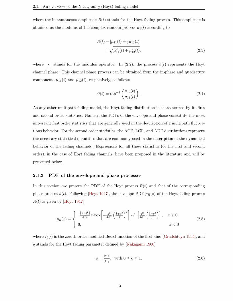
2.1 The PDF pR(z) of the Hoyt fading process R(t) for different values of the fading
parameter q. . . . . . . . . . . . . . . . . . . . . . . . . . . . . . . . . . . . . . . 15
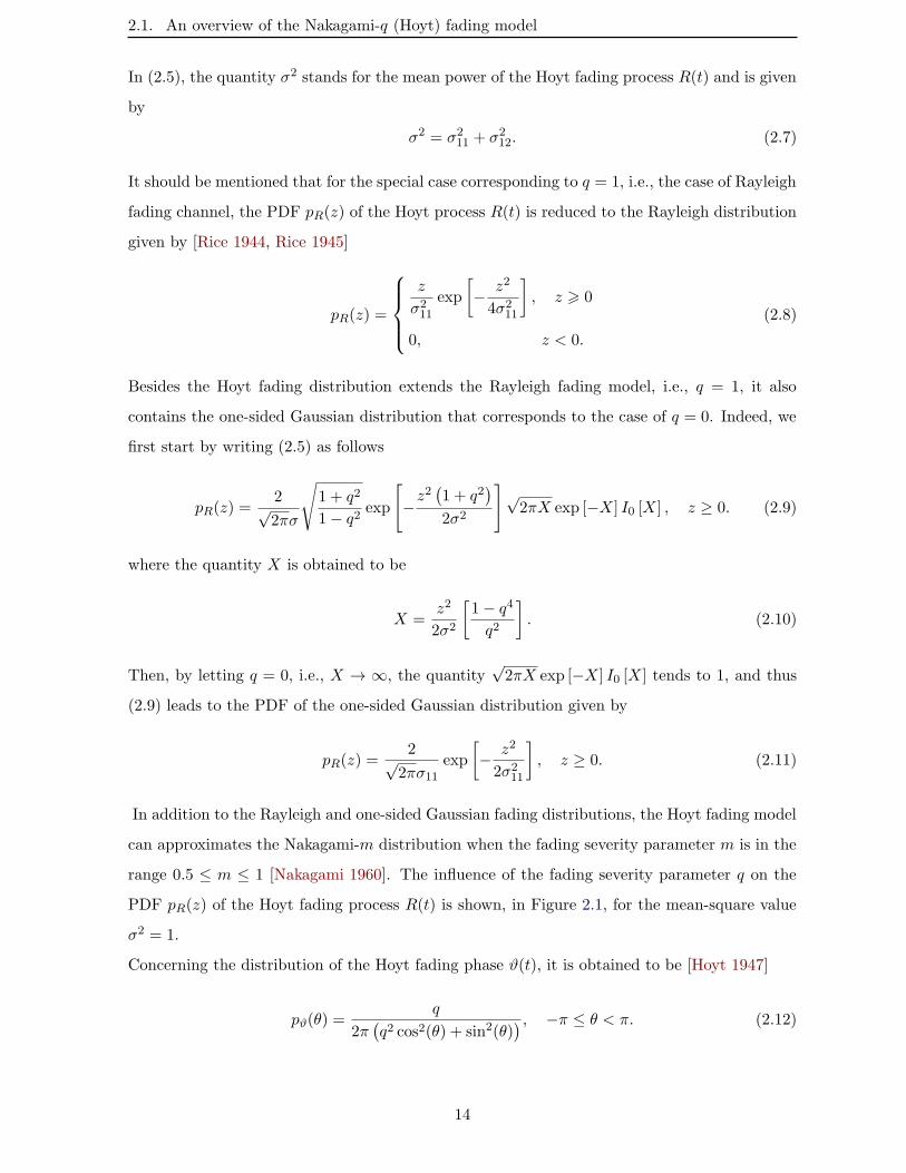
2.2 The PDF pϑ(θ) of the Hoyt phase process ϑ(t) for different values of the fading
parameter q. . . . . . . . . . . . . . . . . . . . . . . . . . . . . . . . . . . . . . . 15
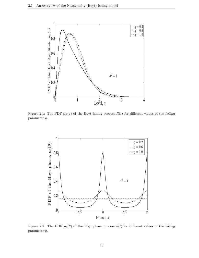
2.3 The ACF Γµ11µ11(τ) of the Gaussian process µ11(t) for the Jakes’ model and
different values of the fading parameter q. . . . . . . . . . . . . . . . . . . . . . . 17
2.4 The Jakes Doppler PSD Sµ11µ11(f) of the Gaussian process µ11(t) for different
values of the fading parameter q. . . . . . . . . . . . . . . . . . . . . . . . . . . . 18
2.5 The normalized LCR NR(r)/fmax1 of the Hoyt fading process R(t) for different
values of the fading parameter q. . . . . . . . . . . . . . . . . . . . . . . . . . . . 19
2.6 The normalized ADF TR−(r) · fmax1 of the Hoyt fading process R(t) for different
values of the fading parameter q. . . . . . . . . . . . . . . . . . . . . . . . . . . . 21
2.7 The single-ring scattering model: A typical M2M single Rayleigh propagation
path from the MST to the MSR. . . . . . . . . . . . . . . . . . . . . . . . . . . . 25
2.8 The double-Doppler ACF of M2M fading channels for various combinations of
the maximum Doppler frequencies fT,max and fR,max. . . . . . . . . . . . . . . . . 26
2.9 The M2M double-Doppler PSD for various combinations of the maximum
Doppler frequencies fT,max and fR,max. . . . . . . . . . . . . . . . . . . . . . . . . 27
2.10 The LCR of M2M single Rayleigh fading channels for various combinations of
the maximum Doppler frequencies fT,max and fR,max. . . . . . . . . . . . . . . . . 28
2.11 The ADF of M2M single Rayleigh fading channels for various combinations of
the maximum Doppler frequencies fT,max and fR,max. . . . . . . . . . . . . . . . . 28
2.12 The double-ring scattering model: M2M single Rayleigh propagation paths from
the MST to the MSR. . . . . . . . . . . . . . . . . . . . . . . . . . . . . . . . . . 29
2.13 The PDF pRD(z) of the double Rayleigh process RD(t) for various combinations
of the mean powers σ2D1and σ2D2
. . . . . . . . . . . . . . . . . . . . . . . . . . . 32
2.14 Amplify-and-forward relay fading model. . . . . . . . . . . . . . . . . . . . . . . 33
3.1 Digital FSK system model with LDI detection. . . . . . . . . . . . . . . . . . . . 35
3.2 The PDF p∆ϑ(ϕ) for various values of the normalized ACF ρτ1 . . . . . . . . . . . 40
3.3 The PDF p∆ϑ(ϕ) for various values of the Hoyt fading parameter q. . . . . . . . 41
xvi
List of Figures
3.4 The average number of FM clicks N for various combinations of the maximum
Doppler frequency fmax1 . . . . . . . . . . . . . . . . . . . . . . . . . . . . . . . . 45
3.5 The average number of FM clicks N for various values of the fading parameter q. 46
3.6 The BEP PE for various values of the Hoyt fading parameter q. . . . . . . . . . . 46
3.7 The BEP PE for various values of BT . . . . . . . . . . . . . . . . . . . . . . . . . 47
4.1 Block diagram of digital communication systems over Hoyt fading channels. . . . 50
4.2 Phasor diagram of a modulated Hoyt faded signal contaminated by Gaussian noise. 51
4.3 Deterministic simulation model for the process µ1i(t). . . . . . . . . . . . . . . . 57
4.4 The PDF p∆Ω(ϕ) for various values of the ACF Γnn(T ). . . . . . . . . . . . . . . 59
4.5 The PDF p∆Ω(ϕ) for various values of the Hoyt fading parameter q. . . . . . . . 59
4.6 The PDF p∆Ω(ϕ) for various values of the parameter Λ. . . . . . . . . . . . . . . 60
4.7 The PDF p∆Ω(ϕ) for different combinations of the maximum Doppler frequencies
fT,max and fR,max. . . . . . . . . . . . . . . . . . . . . . . . . . . . . . . . . . . . 60
5.1 Binary DPSK receiver . . . . . . . . . . . . . . . . . . . . . . . . . . . . . . . . . 63
5.2 The PDF p∆ψ(ϕ) of the overall phase difference ∆ψ for various values of the
Hoyt fading parameter q. . . . . . . . . . . . . . . . . . . . . . . . . . . . . . . . 65
5.3 A comparison between the ACF Γµ12µ12(τ) of the M2M single Hoyt reference
model and that of deterministic model Γµ12µ12(τ). . . . . . . . . . . . . . . . . . 67
5.4 Theoretical and simulated BEP performance of binary noncoherent DPSK for
various values of the Hoyt fading parameter q. . . . . . . . . . . . . . . . . . . . 68
5.5 Theoretical and simulated BEP performance of binary noncoherent DPSK for
different values of the ratio of the maximum Doppler frequencies α. . . . . . . . . 69
5.6 Theoretical and simulated BEP performance of binary noncoherent DPSK over
conventional (α = 0) and M2M (α = 1) channels for different values of the
Doppler frequency fT,max. . . . . . . . . . . . . . . . . . . . . . . . . . . . . . . . 69
5.7 FSK receiver with LDI detection. . . . . . . . . . . . . . . . . . . . . . . . . . . . 70
5.8 BEP performance of the FSK modulation scheme with an LDI detection for
various values of the Hoyt fading parameter q. . . . . . . . . . . . . . . . . . . . 72
5.9 BEP performance of the FSK modulation scheme with an LDI detection for
various values of BT . . . . . . . . . . . . . . . . . . . . . . . . . . . . . . . . . . . 73
5.10 BEP performance of the FSK modulation scheme with an LDI detection for
various combinations of the maximum Doppler frequencies fT,max and fR,max. . . 73
5.11 FSK receiver with differential detection. . . . . . . . . . . . . . . . . . . . . . . . 74
xvii
List of Figures
5.12 A comparison between the BEP of the FSK differential and LDI detectors for
different values of the Hoyt fading parameter q. . . . . . . . . . . . . . . . . . . . 77
5.13 A comparison between the BEP of the FSK differential and LDI detectors for
h = 0.5 and different values of BT . . . . . . . . . . . . . . . . . . . . . . . . . . 77
5.14 A comparison between the BEP of the FSK differential and LDI detectors for
h = 0.7 and different values of BT . . . . . . . . . . . . . . . . . . . . . . . . . . . 78
5.15 A comparison between the BEP of the FSK differential and LDI detectors for
h = 1.0 and different values of BT . . . . . . . . . . . . . . . . . . . . . . . . . . . 78
5.16 A comparison between the BEP of the FSK differential and LDI detectors for
various combination of the maximum Doppler frequencies fT,max and fR,max. . . 79
6.1 Double Hoyt communication scenario. . . . . . . . . . . . . . . . . . . . . . . . . 83
6.2 Deterministic simulation model for the process µij(t). . . . . . . . . . . . . . . . 94
6.3 The envelope PDF pΞ (z) of double Hoyt fading channels. . . . . . . . . . . . . . 95
6.4 The envelope PDF pΞ (z) of the double Hoyt process Ξ(t) for various values of
the Hoyt fading parameters q1 and q2 (q1 = q2). . . . . . . . . . . . . . . . . . . . 96
6.5 The phase PDF pΘ (θ) of the process Θ(t) for various values of the Hoyt fading
parameters q1 and q2. . . . . . . . . . . . . . . . . . . . . . . . . . . . . . . . . . 96
6.6 The LCR NΞ(r) of the double Hoyt process Ξ(t) for various values of the Hoyt
fading parameters q1 and q2. . . . . . . . . . . . . . . . . . . . . . . . . . . . . . . 97
6.7 The ADF TΞ−(r) of the double Hoyt process Ξ(t) for various values of the Hoyt
fading parameters q1 and q2. . . . . . . . . . . . . . . . . . . . . . . . . . . . . . . 97
6.8 The PDF pC (c) of the capacity of double Hoyt fading channels for various values
of q1 and q2. . . . . . . . . . . . . . . . . . . . . . . . . . . . . . . . . . . . . . . . 99
6.9 The CDF FC (c) of the capacity of double Hoyt fading channels for various values
of q1 and q2. . . . . . . . . . . . . . . . . . . . . . . . . . . . . . . . . . . . . . . . 99
6.10 The LCR NC (c) of the capacity of double Hoyt fading channels for various values
of q1 and q2. . . . . . . . . . . . . . . . . . . . . . . . . . . . . . . . . . . . . . . . 100
6.11 The ADF TC (c) of the capacity of double Hoyt fading channels for various values
of q1 and q2. . . . . . . . . . . . . . . . . . . . . . . . . . . . . . . . . . . . . . . . 100
7.1 Structure of the deterministic simulation system for the double Hoyt process Ξ(t).108
7.2 The theoretical and simulated BEP performance of a coherent BPSK modulation
in the double Hoyt fading channels. . . . . . . . . . . . . . . . . . . . . . . . . . . 109
xviii
List of Figures
7.3 The theoretical BEP performance of coherent BPSK, QPSK, FSK, and MSK
modulation schemes in Rayleigh×Hoyt fading channel. . . . . . . . . . . . . . . . 109
7.4 The theoretical BEP performance of a coherent FSK modulation scheme in
Rayleigh×one-sided Gaussian, Rayleigh×Hoyt, and double Rayleigh fading chan-
nels. . . . . . . . . . . . . . . . . . . . . . . . . . . . . . . . . . . . . . . . . . . . 110
7.5 The theoretical BEP performance of a coherent MSK modulation scheme in
Rayleigh×one-sided Gaussian, Rayleigh×Hoyt, and double Rayleigh fading chan-
nels. . . . . . . . . . . . . . . . . . . . . . . . . . . . . . . . . . . . . . . . . . . . 110
xix

List of Tables
7.1 The value of the parameter p for different modulation schemes. . . . . . . . . . . 105
xx
Chapter 1
Introduction
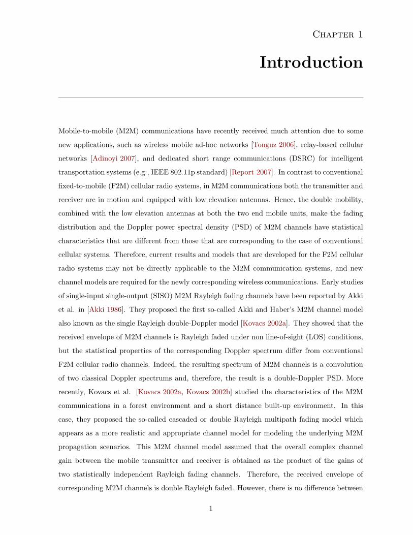
Mobile-to-mobile (M2M) communications have recently received much attention due to some
new applications, such as wireless mobile ad-hoc networks [Tonguz 2006], relay-based cellular
networks [Adinoyi 2007], and dedicated short range communications (DSRC) for intelligent
transportation systems (e.g., IEEE 802.11p standard) [Report 2007]. In contrast to conventional
fixed-to-mobile (F2M) cellular radio systems, in M2M communications both the transmitter and
receiver are in motion and equipped with low elevation antennas. Hence, the double mobility,
combined with the low elevation antennas at both the two end mobile units, make the fading
distribution and the Doppler power spectral density (PSD) of M2M channels have statistical
characteristics that are different from those that are corresponding to the case of conventional
cellular systems. Therefore, current results and models that are developed for the F2M cellular
radio systems may not be directly applicable to the M2M communication systems, and new
channel models are required for the newly corresponding wireless communications. Early studies
of single-input single-output (SISO) M2M Rayleigh fading channels have been reported by Akki
et al. in [Akki 1986]. They proposed the first so-called Akki and Haber’s M2M channel model
also known as the single Rayleigh double-Doppler model [Kovacs 2002a]. They showed that the
received envelope of M2M channels is Rayleigh faded under non line-of-sight (LOS) conditions,
but the statistical properties of the corresponding Doppler spectrum differ from conventional
F2M cellular radio channels. Indeed, the resulting spectrum of M2M channels is a convolution
of two classical Doppler spectrums and, therefore, the result is a double-Doppler PSD. More
recently, Kovacs et al. [Kovacs 2002a, Kovacs 2002b] studied the characteristics of the M2M
communications in a forest environment and a short distance built-up environment. In this
case, they proposed the so-called cascaded or double Rayleigh multipath fading model which
appears as a more realistic and appropriate channel model for modeling the underlying M2M
propagation scenarios. This M2M channel model assumed that the overall complex channel
gain between the mobile transmitter and receiver is obtained as the product of the gains of
two statistically independent Rayleigh fading channels. Therefore, the received envelope of
corresponding M2M channels is double Rayleigh faded. However, there is no difference between
1
1. Introduction
the Doppler PSD functions of single and double Rayleigh fading models and, therefore, double
Rayleigh channels are also characterized by the so-called M2M double-Doppler PSD.
Being relatively a new area of research, M2M communication channels pose numerous in-
teresting research problems. Specifically, for both an effective M2M communication systems
design and a related performance analysis, the appropriate propagation characteristics have to
be taken into account. In this respect, several papers dealing with the performance investiga-
tion of the M2M radio links have appeared in the literature. One of the earliest works has been
reported in [Akki 1994a], where the impact of the double-Doppler spectrum of the M2M single
Rayleigh fading channels on the BEP performance of the FSK modulation has been studied.
In [Hagras 2001], we have presented a comparison study on the performance of the Gaussian
minimum-shift keying (GMSK) modulation with the center sampling differential detection and
center sampling double differential detection schemes over the M2M Rayleigh fading channels
taking into account the random frequency shifts and the co-channel interference. The effect of
the double-Doppler PSD on the BEP performance of the differential quadrature PSK modula-
tion scheme over frequency flat M2M single Rayleigh channels has been studied in [Ali 2007].
In the context of double scattering channels, an expression for the symbol error probability of
some common communication schemes over the so-called double Rayleigh fading channels has
been derived [Salo 2006a]. Concerning also this M2M channel model, Uysal et al. [Uysal 2006]
presented an exact expression for the pair wise error probability of the space-time trellis codes.
The moment generating function and average BEP of M -ary phase-shift keying (M -PSK) mod-
ulation with a maximum ratio combining (MRC) diversity over double Rician fading channels
have been presented in [Wongtrairat 2008]. The performance analysis problem of M2M ra-
dio links has also been addressed in [Wongtrairat 2009] under the double Nakagami-m fading
distribution and for the case of the MRC diversity based receivers.
Besides the channel models described above, the Nakagami-q (Hoyt) distribution is a widely
accepted statistical model for characterizing the short-term multipath effects [Hoyt 1947]. This
fading channel, originally introduced by Nakagami [Nakagami 1960] and Hoyt [Hoyt 1947], in-
cludes the one-sided Gaussian and Rayleigh distributions as special cases. In addition, this
generic model is known to approximate the Nakagami-m model if the severity fading parameter
m is between 0.5 and 1 [Nakagami 1960]. Given the importance of the Hoyt channel distribution
in a statistical modeling of the short-term multipath fading, it is of a great interest, therefore, to
study and analyze its impact on the performance of the wireless M2M communication systems.
To the best of our knowledge, there exists no investigation on this topic so far. The present the-
sis work aims at studying and analyzing the performance of the wireless M2M communication
2
1.1. Thesis Objectives and contributions
systems over Hoyt multipath fading channels.
Namely, the objective of this thesis is to contribute to the topic of performance analysis of
various digital modulation schemes commonly used in wireless communication systems over the
M2M Hoyt fading channels.
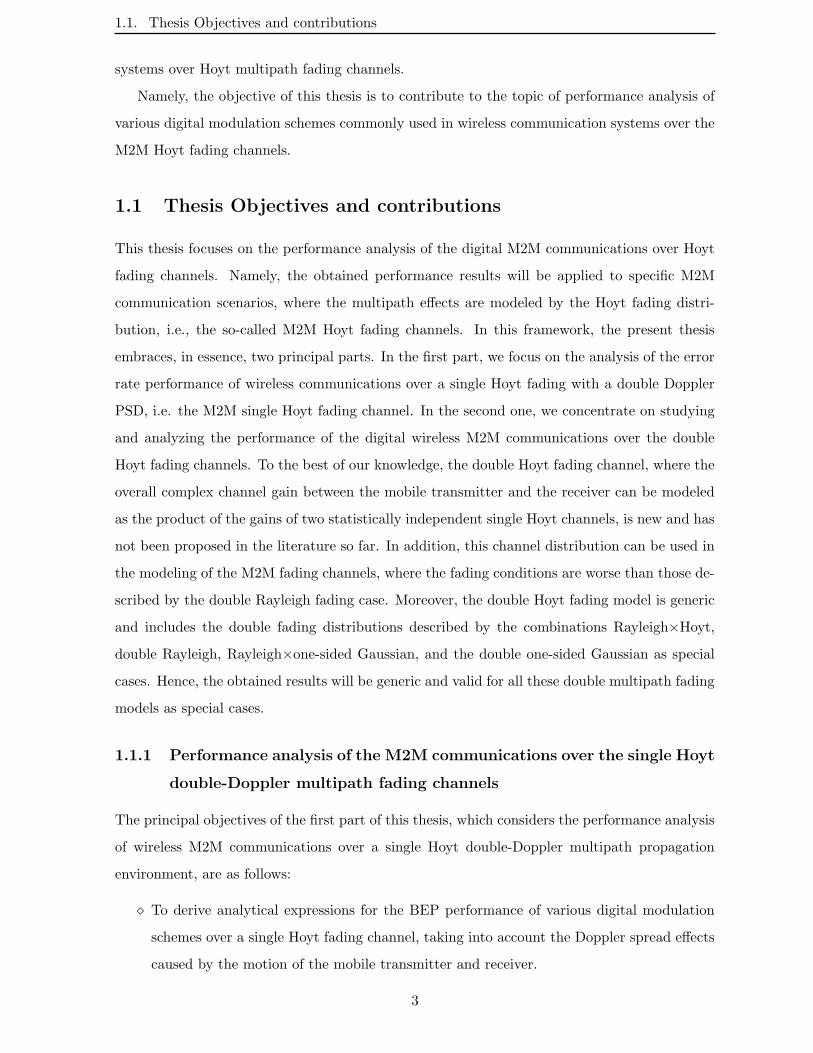
1.1 Thesis Objectives and contributions
This thesis focuses on the performance analysis of the digital M2M communications over Hoyt
fading channels. Namely, the obtained performance results will be applied to specific M2M
communication scenarios, where the multipath effects are modeled by the Hoyt fading distri-
bution, i.e., the so-called M2M Hoyt fading channels. In this framework, the present thesis
embraces, in essence, two principal parts. In the first part, we focus on the analysis of the error
rate performance of wireless communications over a single Hoyt fading with a double Doppler
PSD, i.e. the M2M single Hoyt fading channel. In the second one, we concentrate on studying
and analyzing the performance of the digital wireless M2M communications over the double
Hoyt fading channels. To the best of our knowledge, the double Hoyt fading channel, where the
overall complex channel gain between the mobile transmitter and the receiver can be modeled
as the product of the gains of two statistically independent single Hoyt channels, is new and has
not been proposed in the literature so far. In addition, this channel distribution can be used in
the modeling of the M2M fading channels, where the fading conditions are worse than those de-
scribed by the double Rayleigh fading case. Moreover, the double Hoyt fading model is generic
and includes the double fading distributions described by the combinations Rayleigh×Hoyt,
double Rayleigh, Rayleigh×one-sided Gaussian, and the double one-sided Gaussian as special
cases. Hence, the obtained results will be generic and valid for all these double multipath fading
models as special cases.
1.1.1 Performance analysis of the M2M communications over the single Hoyt
double-Doppler multipath fading channels
The principal objectives of the first part of this thesis, which considers the performance analysis
of wireless M2M communications over a single Hoyt double-Doppler multipath propagation
environment, are as follows:
To derive analytical expressions for the BEP performance of various digital modulation
schemes over a single Hoyt fading channel, taking into account the Doppler spread effects
caused by the motion of the mobile transmitter and receiver.
3
1.1. Thesis Objectives and contributions
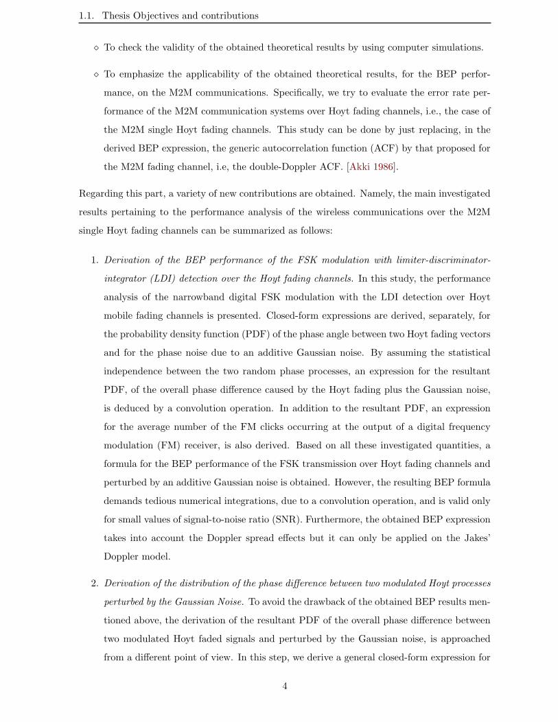
To check the validity of the obtained theoretical results by using computer simulations.
To emphasize the applicability of the obtained theoretical results, for the BEP perfor-
mance, on the M2M communications. Specifically, we try to evaluate the error rate per-
formance of the M2M communication systems over Hoyt fading channels, i.e., the case of
the M2M single Hoyt fading channels. This study can be done by just replacing, in the
derived BEP expression, the generic autocorrelation function (ACF) by that proposed for
the M2M fading channel, i.e, the double-Doppler ACF. [Akki 1986].
Regarding this part, a variety of new contributions are obtained. Namely, the main investigated
results pertaining to the performance analysis of the wireless communications over the M2M
single Hoyt fading channels can be summarized as follows:
1. Derivation of the BEP performance of the FSK modulation with limiter-discriminator-
integrator (LDI) detection over the Hoyt fading channels. In this study, the performance
analysis of the narrowband digital FSK modulation with the LDI detection over Hoyt
mobile fading channels is presented. Closed-form expressions are derived, separately, for
the probability density function (PDF) of the phase angle between two Hoyt fading vectors
and for the phase noise due to an additive Gaussian noise. By assuming the statistical
independence between the two random phase processes, an expression for the resultant
PDF, of the overall phase difference caused by the Hoyt fading plus the Gaussian noise,
is deduced by a convolution operation. In addition to the resultant PDF, an expression
for the average number of the FM clicks occurring at the output of a digital frequency
modulation (FM) receiver, is also derived. Based on all these investigated quantities, a
formula for the BEP performance of the FSK transmission over Hoyt fading channels and
perturbed by an additive Gaussian noise is obtained. However, the resulting BEP formula
demands tedious numerical integrations, due to a convolution operation, and is valid only
for small values of signal-to-noise ratio (SNR). Furthermore, the obtained BEP expression
takes into account the Doppler spread effects but it can only be applied on the Jakes’
Doppler model.
2. Derivation of the distribution of the phase difference between two modulated Hoyt processes
perturbed by the Gaussian Noise. To avoid the drawback of the obtained BEP results men-
tioned above, the derivation of the resultant PDF of the overall phase difference between
two modulated Hoyt faded signals and perturbed by the Gaussian noise, is approached
from a different point of view. In this step, we derive a general closed-form expression for
4
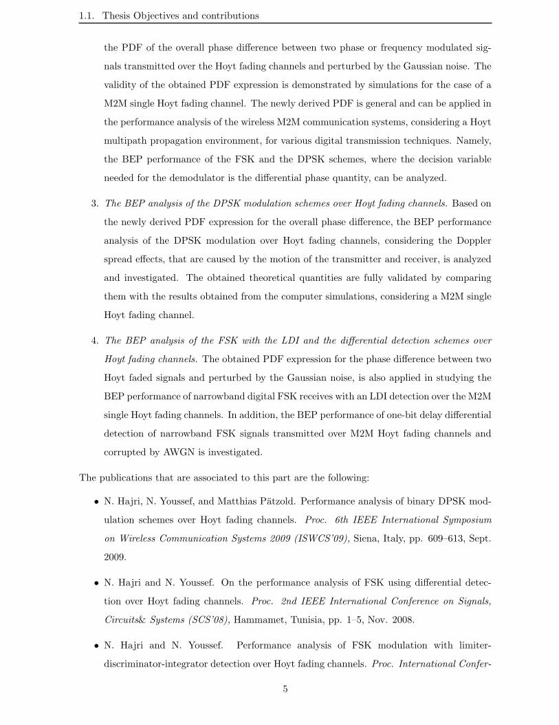
1.1. Thesis Objectives and contributions
the PDF of the overall phase difference between two phase or frequency modulated sig-
nals transmitted over the Hoyt fading channels and perturbed by the Gaussian noise. The
validity of the obtained PDF expression is demonstrated by simulations for the case of a
M2M single Hoyt fading channel. The newly derived PDF is general and can be applied in
the performance analysis of the wireless M2M communication systems, considering a Hoyt
multipath propagation environment, for various digital transmission techniques. Namely,
the BEP performance of the FSK and the DPSK schemes, where the decision variable
needed for the demodulator is the differential phase quantity, can be analyzed.
3. The BEP analysis of the DPSK modulation schemes over Hoyt fading channels. Based on
the newly derived PDF expression for the overall phase difference, the BEP performance
analysis of the DPSK modulation over Hoyt fading channels, considering the Doppler
spread effects, that are caused by the motion of the transmitter and receiver, is analyzed
and investigated. The obtained theoretical quantities are fully validated by comparing
them with the results obtained from the computer simulations, considering a M2M single
Hoyt fading channel.
4. The BEP analysis of the FSK with the LDI and the differential detection schemes over
Hoyt fading channels. The obtained PDF expression for the phase difference between two
Hoyt faded signals and perturbed by the Gaussian noise, is also applied in studying the
BEP performance of narrowband digital FSK receives with an LDI detection over the M2M
single Hoyt fading channels. In addition, the BEP performance of one-bit delay differential
detection of narrowband FSK signals transmitted over M2M Hoyt fading channels and
corrupted by AWGN is investigated.
The publications that are associated to this part are the following:
• N. Hajri, N. Youssef, and Matthias Patzold. Performance analysis of binary DPSK mod-
ulation schemes over Hoyt fading channels. Proc. 6th IEEE International Symposium
on Wireless Communication Systems 2009 (ISWCS’09), Siena, Italy, pp. 609–613, Sept.
2009.
• N. Hajri and N. Youssef. On the performance analysis of FSK using differential detec-
tion over Hoyt fading channels. Proc. 2nd IEEE International Conference on Signals,
Circuits& Systems (SCS’08), Hammamet, Tunisia, pp. 1–5, Nov. 2008.
• N. Hajri and N. Youssef. Performance analysis of FSK modulation with limiter-
discriminator-integrator detection over Hoyt fading channels. Proc. International Confer-
5

1.1. Thesis Objectives and contributions
ence on Wireless Information Networks and Systems(WINSYS’08), Porto, Portugal, pp.
177–181, Jul. 2008.
• N. Hajri and N. Youssef. On the distribution of the phase difference between two Hoyt
processes perturbed by Gaussian Noise. Proc. Kantaoui Forum 9, Tunisia-Japan Sym-
posium on Society, Science & Technology 2008 (KF9–TJASSST’08), Kantaoui, Sousse,
Tunisia, pp. 1–3, Nov. 2008.
• N. Hajri and N. Youssef. Bit error probability of narrow-band digital FM with limiter-
discriminator-integrator detection in Hoyt mobile radio fading channels. Proc. 18th An-
nual IEEE International Symposium on Personal, Indoor and Mobile Radio Communica-
tions 2007 (PIMRC’07), Greece, Athens, pp. 1–5, Sept. 2007.
1.1.2 Performance analysis of the M2M communications over the double
Hoyt fading channels
The double Hoyt fading model is new and, to the best of our knowledge, this thesis is the first to
investigate a study on this channel model so far. Indeed, there are not any published works so far
on the statistical characterization of the double Hoyt fading channels as well as the investigation
of the error rate performance of the digital transmissions over such scattering cascaded channels.
Hence, in order to contribute to the error rate performance of the M2M communications over
double Hoyt fading channels, the investigation of the basic statistical properties of these fading
channels is also mostly required. Therefore, the main objectives of the second part of this thesis
can be classified as follows:
To study the statistical properties of the double Hoyt fading channels.
To investigate the main statistics of the capacity of the double Hoyt fading channels, based
on the use of the obtained statistics for the double Hoyt fading processes.
To study and analyze the performance of the wireless M2M communications over a double
Hoyt fading channel perturbed by the additive white Gaussian noise (AWGN). Specifically,
we try to derive an analytical expression for the BEP performance of the most commonly
used digital modulation schemes over a such M2M multipath fading channel.
To check the validity of the obtained theoretical results by using the computer simulations.
To achieve all the specified objectives of the second part of our thesis work, numerous important
results have been obtained. These results are:
6
1.1. Thesis Objectives and contributions
1. Derivation of the statistical properties of the double Hoyt fading channels. In this step,
analytical expressions for the mean value, variance, PDF, cumulative distribution function
(CDF), level-crossing rate (LCR), and average duration of fades (ADF) of double Hoyt
fading processes are derived. As it is known, the CDF is useful for studying the outage
probability, which is a performance measure commonly used in wireless communications.
In addition, the LCR (or equivalently the frequency of outages) and ADF (or equivalently
the average outage duration) represent important commonly performance measures of
wireless communication systems that are used to reflect the correlation properties (thus
the second order statistics) of fading channels and provide a dynamic representation of the
system outage performance [Guizani 2004]. Furthermore, in this last step, an expression
for the PDF of the corresponding channel phase is provided. Moreover, the validity of all
the derived quantities is confirmed by computer simulations.
2. Derivation of the statistical properties of the capacity of double Hoyt fading channels.
Apart from the amplitude and phase statistics, and with the growing interest in high
spectrally efficient systems, the investigation and analysis of the dynamical behavior of
the fading channel capacity is becoming an important topic of research. In this step,
analytical expressions for the PDF and CDF of the instantaneous capacity process are
derived. Furthermore, the second order statistics, in the form of the LCR and ADF, are
as well provided. The correctness of all the derived quantities is confirmed by computer
simulations.
3. The BEP analysis of the digital modulation schemes over slowly varying frequency flat
double Hoyt fading channels. A performance analysis of digital modulation schemes over
a slowly varying frequency flat double Hoyt fading channel perturbed by an AWGN is
presented. First, an expression for the PDF of the SNR is derived. Then, based upon
this PDF a general expression for the average BEP of the most common digital coherent
modulation schemes is investigated. Namely, the BEP performance of coherent binary
PSK (BPSK), quadrature phase-shift keying (QPSK), FSK, minimum-shift keying (MSK),
and amplitude-shift keying (ASK) modulation schemes is presented. In addition, the
validity of the obtained theoretical results is demonstrated by comparing them with results
obtained from computer simulations, for some of the modulation schemes used in the
analysis.
The publications that are associated to this part are the following:
7

1.2. Thesis Organization
• N. Hajri, N. Youssef, F. Choubani, and T. Kawabata. BER Performance of M2M com-
munications over double Hoyt fading channels. Proc. 21th Annual IEEE International
Symposium on Personal, Indoor and Mobile Radio Communications 2010 (PIMRC’10),
Istanbul, Turkey, pp. 1–5, Sept. 2010.
• N. Hajri, N. Youssef, and M. Patzold. On the statistical properties of the capacity of
double Hoyt fading channels. Proc. 11th IEEE International Workshop on Signal Pro-
cessing Advances for Wireless Communications 2010 (SPAWC’10), Marrakech, Morocco,
pp. 1–5, Jun. 2010.
• N. Hajri, N. Youssef, and M. Patzold. A study on the statistical properties of double hoyt
fading channels. Proc. 6th IEEE International Symposium on Wireless Communication
Systems 2009 (ISWCS’09), Siena, Italy, pp. 201–205, Sept. 2009.
1.2 Thesis Organization
For the purpose of presenting all the above mentioned results, we have chosen to divide the
thesis into 8 chapters.
Chapter2. This chapter introduces the Hoyt multipath fading model and presents an
overview on the wireless M2M communications channels.
Chapter3. This chapter presents all the details of the derivation of an analytical ex-
pression for the BEP performance of a narrowband digital FSK modulation scheme with an
LDI detection over the Hoyt mobile fading channels, taking into account the Doppler spread of
the Jakes’ model.
Chapter4. In this chapter, we look first at the derivation of a closed-form expression
for the PDF of the phase difference between two phase or frequency modulated signals that
are transmitted over Hoyt fading channels and perturbed by the correlated Gaussian noise.
Then, the comparison of the obtained theoretical results with corresponding simulation ones,
considering a M2M single Hoyt fading channel, are presented.
Chapter5. The BEP performance analysis of the digital wireless communications over
Hoyt multipath fading channels is presented in this chapter. Namely, the BEP of DPSK
8
1.2. Thesis Organization
detection schemes together with that of FSK with LDI and differential detections, considering
a M2M single Hoyt multipath fading channel, are provided.
Chapter6. This chapter starts by studying the first and second order statistics of the
double Hoyt fading channels. Indeed, expressions for the mean value, variance, envelope PDF,
phase PDF, LCR, and ADF of the double Hoyt channels are derived. Then, we concentrate,
in this chapter, on the derivation of the first and second order statistics of the corresponding
channel capacity processes. In this case, analytical expressions for the PDF, CDF, LCR, and
ADF of the capacity of double Hoyt channels are presented. Finally, the validity of all the
derived quantities for the fading and channel capacity processes is confirmed by computer
simulations.
Chapter7. This chapter considers the performance analysis of the M2M radio commu-
nications over double Hoyt fading channels perturbed by AWGN. First, by assuming that
the double Hoyt propagation channel is slowly varying and having the frequency-fat fading
characteristics, the PDF of the instantaneous SNR per bit in the double Hoyt fading channels
is derived. Then, an expression for the BEP performance is investigated for several modulation
schemes commonly used in wireless communication systems. Finally, the validity of the theo-
retical results is also checked by means of computer simulations, for some of the modulation
schemes used in the analysis
Chapter8. This chapter concludes the dissertation. In addition, we outline some possi-
ble future research directions in this chapter.
9
Chapter 2
Literature review
The purpose of this chapter is to review, in Section 2.1, the principal characteristics of the Hoyt
fading channels. Then, Section 2.2 presents an overview on the M2M communication channels.
Finally, Section 2.3 concludes the chapter.
2.1 An overview of the Nakagami-q (Hoyt) fading model
2.1.1 Related studies
The Nakagami-q (Hoyt) fading distribution has been originally introduced by [Hoyt 1947] as
a distribution of the modulus of a complex Gaussian random variable whose components are
uncorrelated with zero-mean and unequal variances. Then, Nakagami et al. [Nakagami 1960]
investigated this model as an approximation for the Nakagami-m fading distribution in the
range of fading that extends from the one-sided Gaussian model to the Rayleigh model. Hence,
the Nakagami-q (Hoyt) model has been sometimes referred to as the Nakagami-Hoyt distribu-
tion [Crepeau 1992]. In [Hoyt 1947], the first order statistics of the Hoyt fading channel have
been derived. Specifically, closed-form expressions for the envelope PDF and phase PDF of
Hoyt fading channels have been presented. Originally, the Hoyt fading model has been used
by [Nakagami 1960] and [Chytil 1967] for modeling radio channels subject to strong ionospheric
scintillation, such as satellite links. Recently, the model is being more and more useful in chan-
nel modeling of multipath fading, where the fading conditions are more severe than those of the
classical Rayleigh case. For instance, in [Youssef 2005a], the crossing statistics of the phase pro-
cesses and random FM noise of the Nakagami-q channel have been studied. In [Youssef 2005b],
the second order statistics of the Hoyt fading channel in terms of the LCR and ADF have been
presented. Besides these statistics, Youssef et al. [Youssef 2005b] showed that the Hoyt fading
model can be applied to realistic mobile satellite channel, in the case of an environment with
heavy shadowing. In dealing with the statistical characterization of the Hoyt fading channels
and given the explosion of interest and research, that is taking place in the area of diversity
reception based on the MRC and equal gain combining (EGC) techniques [Simon 2005], exact
10
2.1. An overview of the Nakagami-q (Hoyt) fading model
form expressions for the LCR and ADF of MRC and EGC diversity systems in the Hoyt fad-
ing environment have been presented in [Fraidenraich 2005]. Recently, in [Stefanovie 2007], a
closed-form expression for the envelope LCR of a cosine signal with a constant amplitude inter-
fered by the Nakagami-q process has been derived. More recently, Ricardo et al. [Ricardo 2008]
investigated an exact closed-form and general expressions for the marginal and joint moments
as well as for the correlation coefficient of the instantaneous powers of two Hoyt signals.
Being relatively an important general multipath fading model, which has been frequently
used in the channel modeling of short-term multipath effects, the Hoyt fading channel has re-
cently gained a widespread attention in the performance analysis of wireless communication
systems. For example, in [Simon 1998, Simon 2005], a unified approach to evaluate the er-
ror rate performance of the digital communication systems operating over a generalized fading
channel, especially a Hoyt fading channel, has been presented. This approach relies on employ-
ing alternative representations of classic functions arising in the error probability analysis of
the digital communication systems (e.g., the Gaussian Q-function and the Marcum Q-function
[Gradshteyn 1994]) in such a manner that the resulting expressions for various performance
measures such as average bit or symbol error rate are in a form that is rarely more complicated
than a single integral with infinite limits and an integrand composed of elementary (e.g., expo-
nential and trigonometric [Gradshteyn 1994]) functions. Similarly, a unified framework for the
error performance of M -ary quadrature amplitude modulation (M -QAM), employing L-branch
EGC and operating over the Hoyt fading channels, has been provided in [Karagiannidis 2005].
By considering M -ary continuous phase modulations (CPM) systems with a differential phase
detection and a MRC, Korn et al. [Korn 2001] analyzed the BEP performance of the underlying
diversity systems in various fading channels, especially for the case of a slowly varying Hoyt
fading channel. In [Liu 2006], a study dealing with the BEP performance of the asynchronous
binary direct sequence (DS) code division multiple access (CDMA) systems operating over fre-
quency flat Hoyt fading channels has been presented. In addition, exact closed-form expressions
for the moments of the SNR at the output of the EGC over Hoyt fading channels have been
derived by Zogas et al. [Zogas 2005]. In a recent work, Iskander et al. [Iskander 2008] inves-
tigated the derivation of an expression for the average symbol error probability (ASEP) of an
EGC receiver. However, their presented results have been limited to dual-diversity case only.
To avoid the drawback of the above obtained results, Baid et al. [Baid 2008] studied the general
case by considering an arbitrary number of diversity branches and analyzed the performance of
a predetection EGC receiver in independent Hoyt fading channels. Hence, mathematical expres-
sions for the average output SNR and the average bit error rate (ABER) have been provided
11

2.1. An overview of the Nakagami-q (Hoyt) fading model
for coherent BPSK, FSK, DPSK, and noncoherent FSK modulation schemes. More recently,
Radaydeh et al. [Radaydeh 2008b] derived exact form expressions for the average error perfor-
mance of M -ary orthogonal signals (such as M -FSK) with noncoherent EGC diversity systems
in non-identical generalized Rayleigh, Rician, Nakagami-m, and implicitly Nakagami-q fading
channels. Within the framework of the error rate performance of the digital transmission over
the Hoyt multipath fading channels, Radaydeh et al. derived, in [Radaydeh 2007], exact form
expressions for the ASEP of SISO systems using M -ary modulation schemes. Excited by the
importance and the much research activity on systems with multiple antennas at the trans-
mitter or the receiver or at both, closed-form expressions for the ASEP of binary and M -ary
modulated signals transmitted over single-input multiple-output (SIMO) and multiple-input
multiple-output (MIMO) Hoyt diversity systems have been derived in [Duong 2007]. To reflect
a real noncoherent receiver with a diversity reception for binary orthogonal signals transmitted
over a Hoyt fading channel, Radaydeh et al. [Radaydeh 2008a] assumed that the multipath
fading model is a non-identical Nakagami-q fading channel. In this case, the average fading
powers and the fading parameters take arbitrary values among diversity branches. Based on
this assumption, the BEP performance of the obtained realistic diversity receiver operating over
Hoyt fading channels has been presented, in terms of elementary functions. From the literature
above, it is worth noting that the Hoyt fading channel is being used more frequently in the
channel modelling and performance analysis related to mobile radio communications. In the
following, we present the main statistical properties of this fading channel model.
2.1.2 An elementary description
In general, the Hoyt channel gain is often modeled, in the equivalent complex baseband repre-
sentation, by a zero-mean complex Gaussian process µ1(t) given by [Hoyt 1947]
µ1(t) = µ11(t) + jµ12(t) (2.1)
where µ11(t) and µ12(t) are uncorrelated zero-mean Gaussian processes with different variances
σ211 and σ212, respectively. The complex channel gain µ1(t) can also be expressed as
µ1(t) = R(t) exp [jϑ(t)] (2.2)
12
2.1. An overview of the Nakagami-q (Hoyt) fading model
where the instantaneous amplitude R(t) stands for the Hoyt fading process. This amplitude is
obtained as the modulus of the complex random process µ1(t) according to
R(t) = |µ11(t) + jµ12(t)|
=√µ211(t) + µ212(t). (2.3)
where | · | stands for the modulus operator. In (2.2), the process ϑ(t) represents the Hoyt
channel phase. This channel phase process can be obtained from the in-phase and quadrature
components µ11(t) and µ12(t), respectively, as follows
ϑ(t) = tan−1
(µ12(t)
µ11(t)
). (2.4)
As any other multipath fading model, the Hoyt fading distribution is characterized by its first
and second order statistics. Namely, the PDFs of the envelope and phase constitute the most
important first order statistics that are generally used in the description of a multipath fluctua-
tions behavior. For the second order statistics, the ACF, LCR, and ADF distributions represent
the necessary statistical quantities that are commonly used in the description of the dynamical
behavior of the fading channels. Expressions for all these statistics (of the first and second
order), in the case of Hoyt fading channels, have been proposed in the literature and will be
presented below.
2.1.3 PDF of the envelope and phase processes
In this section, we present the PDF of the Hoyt process R(t) and that of the corresponding
phase process ϑ(t). Following [Hoyt 1947], the envelope PDF pR(z) of the Hoyt fading process
R(t) is given by [Hoyt 1947]
pR(z) =
(1+q2)σ2q
z exp
[− z2
4σ2
(1+q2
q
)2]· I0[z2
4σ2
(1−q4
q2
)], z > 0
0, z < 0
(2.5)
where I0(·) is the zeroth-order modified Bessel function of the first kind [Gradshteyn 1994], and
q stands for the Hoyt fading parameter defined by [Nakagami 1960]
q =σ12σ11
, with 0 ≤ q ≤ 1. (2.6)
13
2.1. An overview of the Nakagami-q (Hoyt) fading model
In (2.5), the quantity σ2 stands for the mean power of the Hoyt fading process R(t) and is given
by
σ2 = σ211 + σ212. (2.7)
It should be mentioned that for the special case corresponding to q = 1, i.e., the case of Rayleigh
fading channel, the PDF pR(z) of the Hoyt process R(t) is reduced to the Rayleigh distribution
given by [Rice 1944, Rice 1945]
pR(z) =
z
σ211exp
[− z2
4σ211
], z > 0
0, z < 0.
(2.8)
Besides the Hoyt fading distribution extends the Rayleigh fading model, i.e., q = 1, it also
contains the one-sided Gaussian distribution that corresponds to the case of q = 0. Indeed, we
first start by writing (2.5) as follows
pR(z) =2√2πσ
√1 + q2
1− q2exp
[−z
2(1 + q2
)
2σ2
]√2πX exp [−X] I0 [X] , z ≥ 0. (2.9)
where the quantity X is obtained to be
X =z2
2σ2
[1− q4
q2
]. (2.10)
Then, by letting q = 0, i.e., X → ∞, the quantity√2πX exp [−X] I0 [X] tends to 1, and thus
(2.9) leads to the PDF of the one-sided Gaussian distribution given by
pR(z) =2√
2πσ11exp
[− z2
2σ211
], z ≥ 0. (2.11)
In addition to the Rayleigh and one-sided Gaussian fading distributions, the Hoyt fading model
can approximates the Nakagami-m distribution when the fading severity parameter m is in the
range 0.5 ≤ m ≤ 1 [Nakagami 1960]. The influence of the fading severity parameter q on the
PDF pR(z) of the Hoyt fading process R(t) is shown, in Figure 2.1, for the mean-square value
σ2 = 1.
Concerning the distribution of the Hoyt fading phase ϑ(t), it is obtained to be [Hoyt 1947]
pϑ(θ) =q
2π(q2 cos2(θ) + sin2(θ)
) , −π ≤ θ < π. (2.12)
14
2.1. An overview of the Nakagami-q (Hoyt) fading model
0 1 2 3 40
0.2
0.4
0.6
0.8
1
Level, z
PD
Fof
th
eH
oyt
Ap
mli
tu
de,pR
(z)
q = 0.2q = 0.6q = 1.0
σ2 = 1
Figure 2.1: The PDF pR(z) of the Hoyt fading process R(t) for different values of the fadingparameter q.
0
0.2
0.4
0.6
0.8
1
Phase, θ
PD
Fof
the
Hoyt
phase,pϑ(θ)
q = 0.2
q = 0.6
q = 1.0
−π −π/2 0 π/2 π
σ2 = 1
Figure 2.2: The PDF pϑ(θ) of the Hoyt phase process ϑ(t) for different values of the fadingparameter q.
15

2.1. An overview of the Nakagami-q (Hoyt) fading model
As expected, when q = 1, i.e., the case of Rayleigh fading channels, (2.12) yields to a uniform
distribution over [−π, π). The effect of the parameter q on the phase PDF pϑ(θ) of the Hoyt
fading channel can be studied from Figure 2.2.
2.1.4 Second order statistics
2.1.4.1 Autocorrelation function
An important statistical characteristic of the in-phase and quadrature random processes µ11(t)
and µ12(t), respectively, is their ACF. Indeed, with a simple calculation and analysis of the ACF
of these processes, we can determinate how quickly each corresponding random process changes
with respect to the time function. The ACF of the zero-mean Gaussian process µ1i(t) (i = 1, 2)
represents the expected value of the product of the signal µ1i(t) at a time t with a time-shifted
version of itself at a time t + τ , i.e., µ1i(t + τ). Thus, the corresponding ACF Γµ1iµ1i(τ) is
defined by
Γµ1iµ1i(τ) = E µ∗1i(t)µ1i(t+ τ) , i = 1, 2 (2.13)
where the superscripted asterisk ∗ denotes the complex conjugation, and E · stands for the
expected value operator. Based on the ACFs Γµ11µ11(τ) and Γµ12µ12(τ) of the processes µ11(t)
and µ12(t), respectively, the ACF of the complex zero-mean Gaussian process µ1(t) in (2.1) can
be written as [Papoulis 2002]
Γµ1µ1(τ) = Γµ11µ11(τ) + Γµ12µ12(τ). (2.14)
An important use of the ACF resides in the fact that the PSD can be directly obtained from it.
The general relation between the PSD Sµ1iµ1i(f) of the process µ1i(t) (i = 1, 2) and the ACF
Γµ1iµ1i(τ) is known as the Wiener-Khinchine relationship [CouchII 2001]. Following Wiener’s
theorem, the PSD Sµ1iµ1i(f) (i = 1, 2) of the random process µ1i(t) is the Fourier transform of
the corresponding ACF Γµ1iµ1i(τ). Thus, Sµ1iµ1i(f) can be written as
Sµ1iµ1i(f) =
∞∫
−∞
Γµ1iµ1i(τ)e−j2πfτdτ, i = 1, 2. (2.15)
The shape of the PSD of the complex channel gain µ1(t) is identical to the Doppler PSD,
which is obtained from both the power of all electromagnetic waves arriving at the receiver
antenna and the distribution of the angles of arrival. In addition to that, the radiation
pattern of the receiving antenna has a decisive influence on the shape of the Doppler PSD
16
2.1. An overview of the Nakagami-q (Hoyt) fading model
0 0.01 0.02 0.03 0.04 0.05−0.4
−0.2
0
0.2
0.4
0.6
0.8
1
Time, τ (s)
AC
Ffo
rJakes’
mod
el,
Γµ
11µ
11(τ)
q = 0.2q = 0.6q = 1.0
σ2 = 1fmax1
= 92 Hz
Figure 2.3: The ACF Γµ11µ11(τ) of the Gaussian process µ11(t) for the Jakes’ model anddifferent values of the fading parameter q.
[Clarke 1968, Jakes 1993, Patzold 2002]. By assuming omnidirectional antennas, we can then
easily calculate the Doppler PSD Sµ1µ1(f) of the scattered component µ1(t). In this case and
following [Clarke 1968, Jakes 1993], the Doppler PSD Sµ1µ1(f) of the complex process µ1(t) can
be expressed as
Sµ1µ1(f) = Sµ11µ11(f) + Sµ12µ12(f) (2.16)
where Sµ1iµ1i(f) corresponds to the Jakes Doppler PSD, which is given by [Clarke 1968]
Sµ1iµ1i(f) =
σ2
1i
πfmaxi
√
1−(f/fmaxi), |f | 6 fmaxi
0, |f | > fmaxi
. (2.17)
In (2.17), fmaxi denotes the maximum Doppler frequency corresponding to the Gaussian process
µ1i(t) (i = 1, 2). The inverse Fourier transform of (2.17) results in the ACF Γµ1iµ1i(τ) of the
process µ1i(t) for the Jakes’ model, which is given by [Jakes 1993]
Γµ1iµ1i(τ) = σ21iJ0 (2πfmaxiτ) , i = 1, 2 (2.18)
where J0 (·) denotes the zeroth-order Bessel function of the first kind [Gradshteyn 1994]. The
shape of the ACF Γµ11µ11(τ) of the process µ11(t) for the Jakes’ model is presented together
17
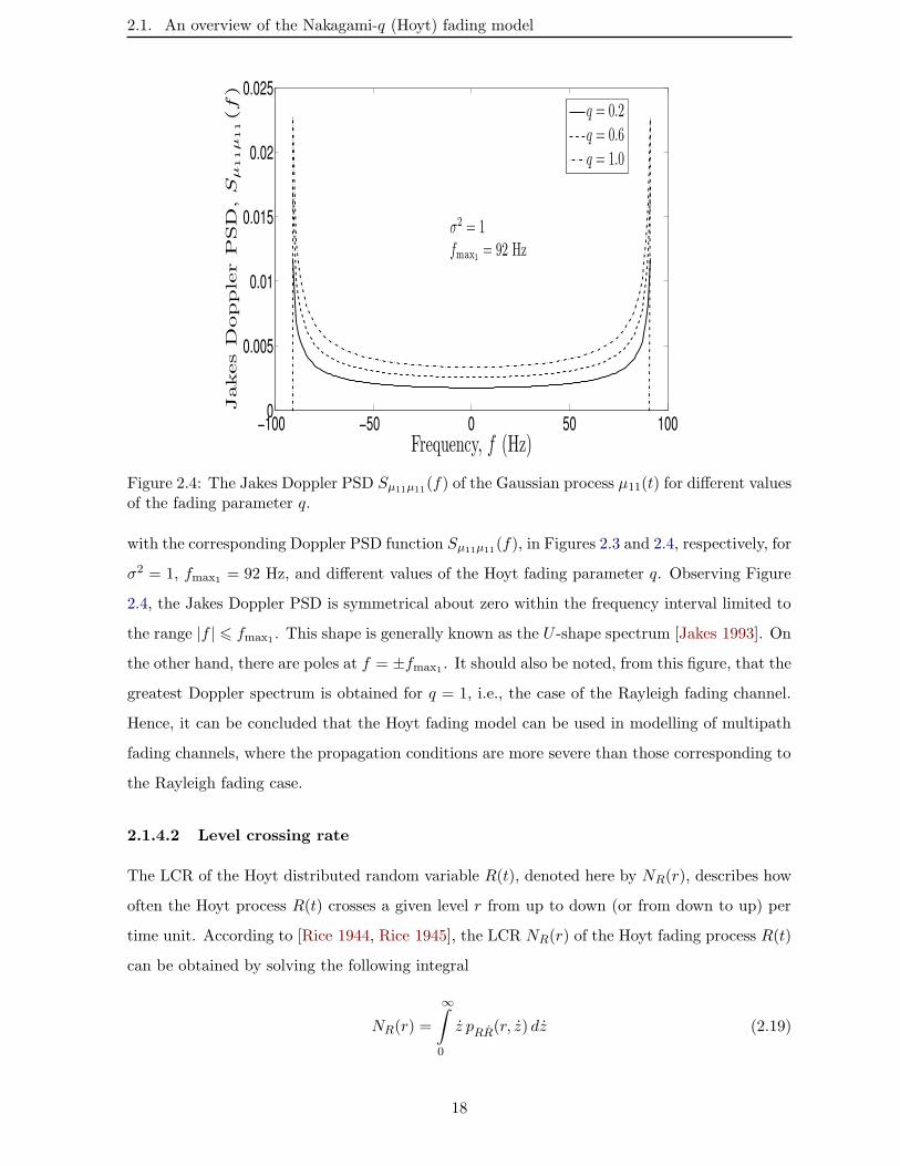
2.1. An overview of the Nakagami-q (Hoyt) fading model
−100 −50 0 50 1000
0.005
0.01
0.015
0.02
0.025
Frequency, f (Hz)
Jakes
Dopple
rP
SD
,Sµ
11µ
11(f
)
q = 0.2
q = 0.6
q = 1.0
σ2 = 1fmax1
= 92 Hz
Figure 2.4: The Jakes Doppler PSD Sµ11µ11(f) of the Gaussian process µ11(t) for different valuesof the fading parameter q.
with the corresponding Doppler PSD function Sµ11µ11(f), in Figures 2.3 and 2.4, respectively, for
σ2 = 1, fmax1 = 92 Hz, and different values of the Hoyt fading parameter q. Observing Figure
2.4, the Jakes Doppler PSD is symmetrical about zero within the frequency interval limited to
the range |f | 6 fmax1 . This shape is generally known as the U -shape spectrum [Jakes 1993]. On
the other hand, there are poles at f = ±fmax1 . It should also be noted, from this figure, that the
greatest Doppler spectrum is obtained for q = 1, i.e., the case of the Rayleigh fading channel.
Hence, it can be concluded that the Hoyt fading model can be used in modelling of multipath
fading channels, where the propagation conditions are more severe than those corresponding to
the Rayleigh fading case.
2.1.4.2 Level crossing rate
The LCR of the Hoyt distributed random variable R(t), denoted here by NR(r), describes how
often the Hoyt process R(t) crosses a given level r from up to down (or from down to up) per
time unit. According to [Rice 1944, Rice 1945], the LCR NR(r) of the Hoyt fading process R(t)
can be obtained by solving the following integral
NR(r) =
∞∫
0
z pRR(r, z) dz (2.19)
18
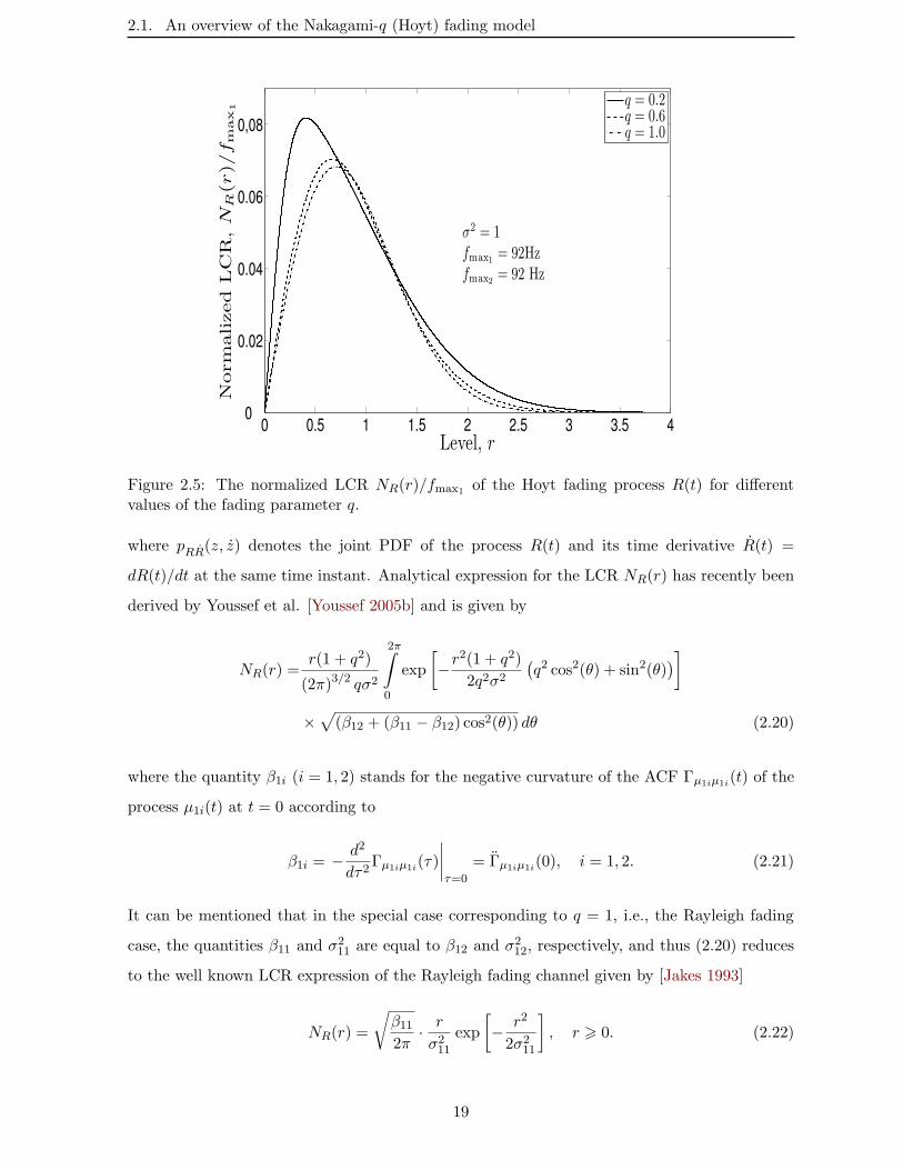
2.1. An overview of the Nakagami-q (Hoyt) fading model
0 0.5 1 1.5 2 2.5 3 3.5 40
0.02
0.04
0.06
0,08
Level, r
Norm
alized
LC
R,NR
(r)/f
max
1
q = 0.2q = 0.6q = 1.0
σ2 = 1fmax1
= 92Hzfmax2
= 92 Hz
Figure 2.5: The normalized LCR NR(r)/fmax1 of the Hoyt fading process R(t) for differentvalues of the fading parameter q.
where pRR(z, z) denotes the joint PDF of the process R(t) and its time derivative R(t) =
dR(t)/dt at the same time instant. Analytical expression for the LCR NR(r) has recently been
derived by Youssef et al. [Youssef 2005b] and is given by
NR(r) =r(1 + q2)
(2π)3/2 qσ2
2π∫
0
exp
[−r
2(1 + q2)
2q2σ2(q2 cos2(θ) + sin2(θ)
)]
×√
(β12 + (β11 − β12) cos2(θ)) dθ (2.20)
where the quantity β1i (i = 1, 2) stands for the negative curvature of the ACF Γµ1iµ1i(t) of the
process µ1i(t) at t = 0 according to
β1i = − d2
dτ2Γµ1iµ1i(τ)
∣∣∣∣τ=0
= Γµ1iµ1i(0), i = 1, 2. (2.21)
It can be mentioned that in the special case corresponding to q = 1, i.e., the Rayleigh fading
case, the quantities β11 and σ211 are equal to β12 and σ212, respectively, and thus (2.20) reduces
to the well known LCR expression of the Rayleigh fading channel given by [Jakes 1993]
NR(r) =
√β112π
· r
σ211exp
[− r2
2σ211
], r > 0. (2.22)
19
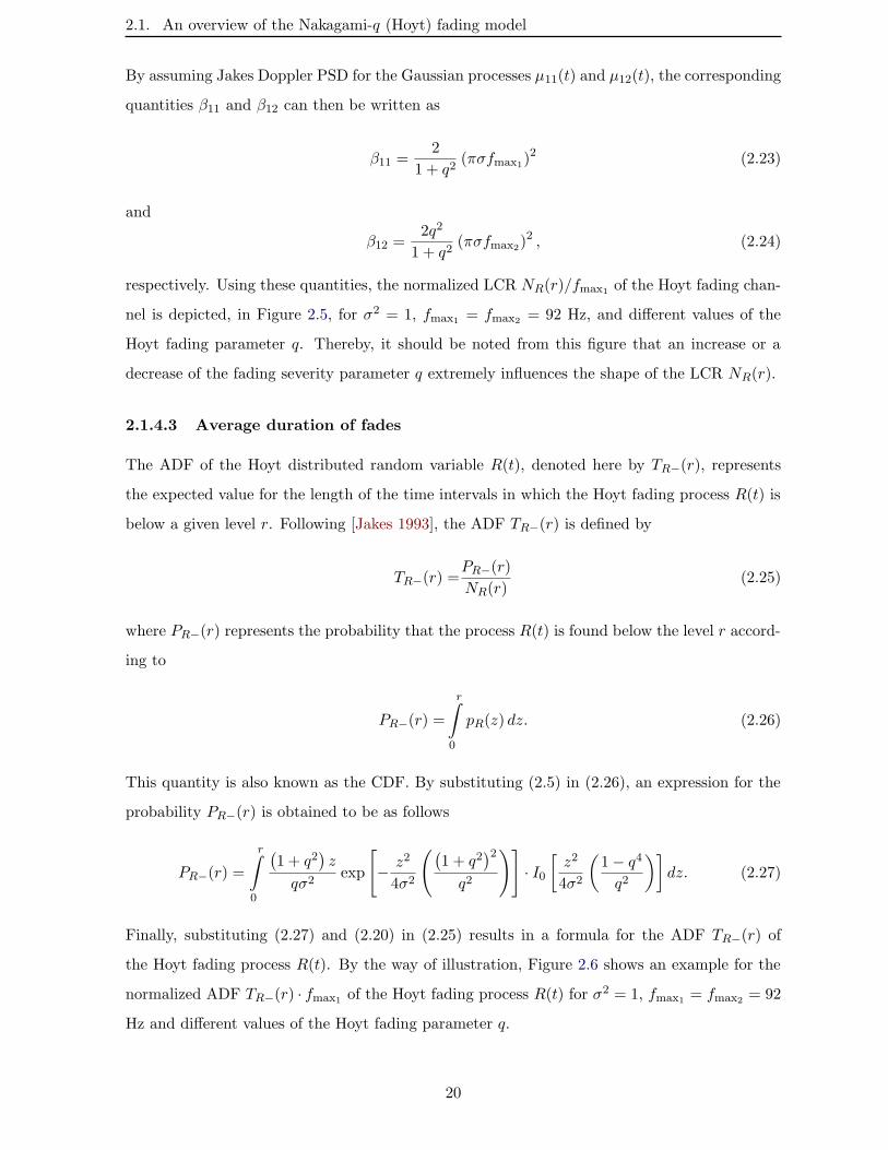
2.1. An overview of the Nakagami-q (Hoyt) fading model
By assuming Jakes Doppler PSD for the Gaussian processes µ11(t) and µ12(t), the corresponding
quantities β11 and β12 can then be written as
β11 =2
1 + q2(πσfmax1)
2 (2.23)
and
β12 =2q2
1 + q2(πσfmax2)
2 , (2.24)
respectively. Using these quantities, the normalized LCR NR(r)/fmax1 of the Hoyt fading chan-
nel is depicted, in Figure 2.5, for σ2 = 1, fmax1 = fmax2 = 92 Hz, and different values of the
Hoyt fading parameter q. Thereby, it should be noted from this figure that an increase or a
decrease of the fading severity parameter q extremely influences the shape of the LCR NR(r).
2.1.4.3 Average duration of fades
The ADF of the Hoyt distributed random variable R(t), denoted here by TR−(r), represents
the expected value for the length of the time intervals in which the Hoyt fading process R(t) is
below a given level r. Following [Jakes 1993], the ADF TR−(r) is defined by
TR−(r) =PR−(r)
NR(r)(2.25)
where PR−(r) represents the probability that the process R(t) is found below the level r accord-
ing to
PR−(r) =
r∫
0
pR(z) dz. (2.26)
This quantity is also known as the CDF. By substituting (2.5) in (2.26), an expression for the
probability PR−(r) is obtained to be as follows
PR−(r) =
r∫
0
(1 + q2
)z
qσ2exp
[− z2
4σ2
((1 + q2
)2
q2
)]· I0[z2
4σ2
(1− q4
q2
)]dz. (2.27)
Finally, substituting (2.27) and (2.20) in (2.25) results in a formula for the ADF TR−(r) of
the Hoyt fading process R(t). By the way of illustration, Figure 2.6 shows an example for the
normalized ADF TR−(r) · fmax1 of the Hoyt fading process R(t) for σ2 = 1, fmax1 = fmax2 = 92
Hz and different values of the Hoyt fading parameter q.
20
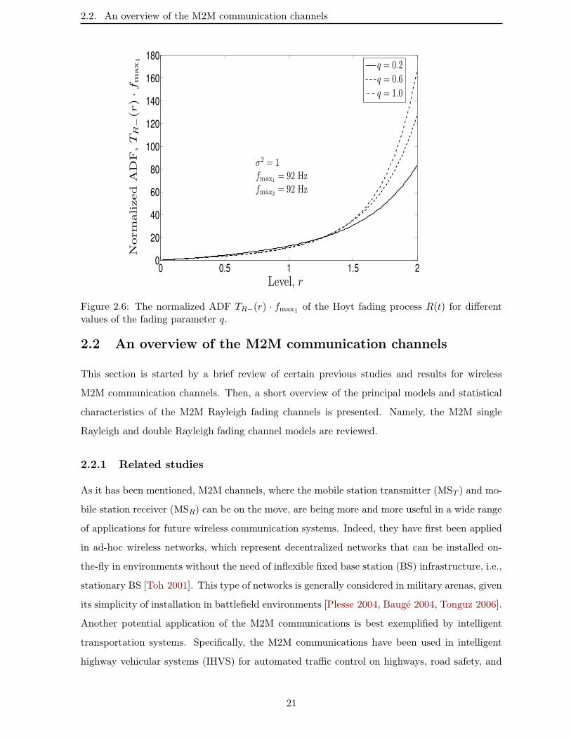
2.2. An overview of the M2M communication channels
0 0.5 1 1.5 20
20
40
60
80
100
120
140
160
180
Level, r
Norm
alized
AD
F,TR−
(r)·f
max
1
q = 0.2
q = 0.6
q = 1.0
σ2 = 1fmax1
= 92 Hzfmax2
= 92 Hz
Figure 2.6: The normalized ADF TR−(r) · fmax1 of the Hoyt fading process R(t) for differentvalues of the fading parameter q.
2.2 An overview of the M2M communication channels
This section is started by a brief review of certain previous studies and results for wireless
M2M communication channels. Then, a short overview of the principal models and statistical
characteristics of the M2M Rayleigh fading channels is presented. Namely, the M2M single
Rayleigh and double Rayleigh fading channel models are reviewed.
2.2.1 Related studies
As it has been mentioned, M2M channels, where the mobile station transmitter (MST ) and mo-
bile station receiver (MSR) can be on the move, are being more and more useful in a wide range
of applications for future wireless communication systems. Indeed, they have first been applied
in ad-hoc wireless networks, which represent decentralized networks that can be installed on-
the-fly in environments without the need of inflexible fixed base station (BS) infrastructure, i.e.,
stationary BS [Toh 2001]. This type of networks is generally considered in military arenas, given
its simplicity of installation in battlefield environments [Plesse 2004, Bauge 2004, Tonguz 2006].
Another potential application of the M2M communications is best exemplified by intelligent
transportation systems. Specifically, the M2M communications have been used in intelligent
highway vehicular systems (IHVS) for automated traffic control on highways, road safety, and
21
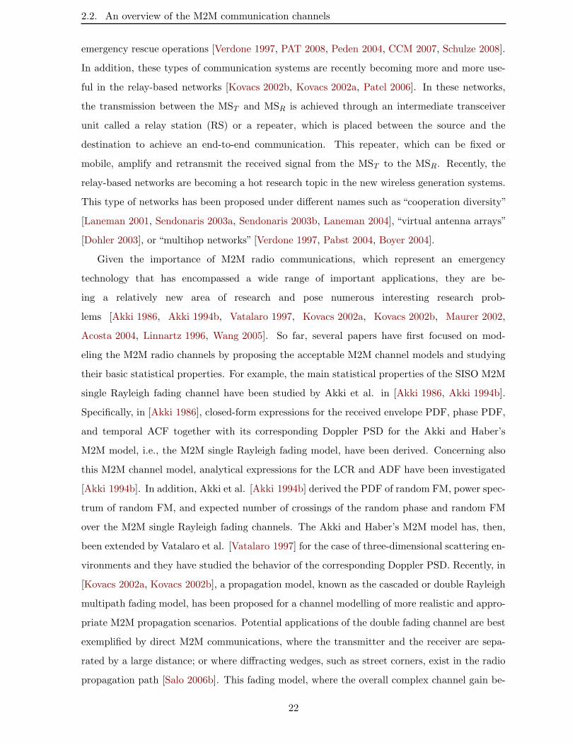
2.2. An overview of the M2M communication channels
emergency rescue operations [Verdone 1997, PAT 2008, Peden 2004, CCM 2007, Schulze 2008].
In addition, these types of communication systems are recently becoming more and more use-
ful in the relay-based networks [Kovacs 2002b, Kovacs 2002a, Patel 2006]. In these networks,
the transmission between the MST and MSR is achieved through an intermediate transceiver
unit called a relay station (RS) or a repeater, which is placed between the source and the
destination to achieve an end-to-end communication. This repeater, which can be fixed or
mobile, amplify and retransmit the received signal from the MST to the MSR. Recently, the
relay-based networks are becoming a hot research topic in the new wireless generation systems.
This type of networks has been proposed under different names such as “cooperation diversity”
[Laneman 2001, Sendonaris 2003a, Sendonaris 2003b, Laneman 2004], “virtual antenna arrays”
[Dohler 2003], or “multihop networks” [Verdone 1997, Pabst 2004, Boyer 2004].
Given the importance of M2M radio communications, which represent an emergency
technology that has encompassed a wide range of important applications, they are be-
ing a relatively new area of research and pose numerous interesting research prob-
lems [Akki 1986, Akki 1994b, Vatalaro 1997, Kovacs 2002a, Kovacs 2002b, Maurer 2002,
Acosta 2004, Linnartz 1996, Wang 2005]. So far, several papers have first focused on mod-
eling the M2M radio channels by proposing the acceptable M2M channel models and studying
their basic statistical properties. For example, the main statistical properties of the SISO M2M
single Rayleigh fading channel have been studied by Akki et al. in [Akki 1986, Akki 1994b].
Specifically, in [Akki 1986], closed-form expressions for the received envelope PDF, phase PDF,
and temporal ACF together with its corresponding Doppler PSD for the Akki and Haber’s
M2M model, i.e., the M2M single Rayleigh fading model, have been derived. Concerning also
this M2M channel model, analytical expressions for the LCR and ADF have been investigated
[Akki 1994b]. In addition, Akki et al. [Akki 1994b] derived the PDF of random FM, power spec-
trum of random FM, and expected number of crossings of the random phase and random FM
over the M2M single Rayleigh fading channels. The Akki and Haber’s M2M model has, then,
been extended by Vatalaro et al. [Vatalaro 1997] for the case of three-dimensional scattering en-
vironments and they have studied the behavior of the corresponding Doppler PSD. Recently, in
[Kovacs 2002a, Kovacs 2002b], a propagation model, known as the cascaded or double Rayleigh
multipath fading model, has been proposed for a channel modelling of more realistic and appro-
priate M2M propagation scenarios. Potential applications of the double fading channel are best
exemplified by direct M2M communications, where the transmitter and the receiver are sepa-
rated by a large distance; or where diffracting wedges, such as street corners, exist in the radio
propagation path [Salo 2006b]. This fading model, where the overall complex channel gain be-
22
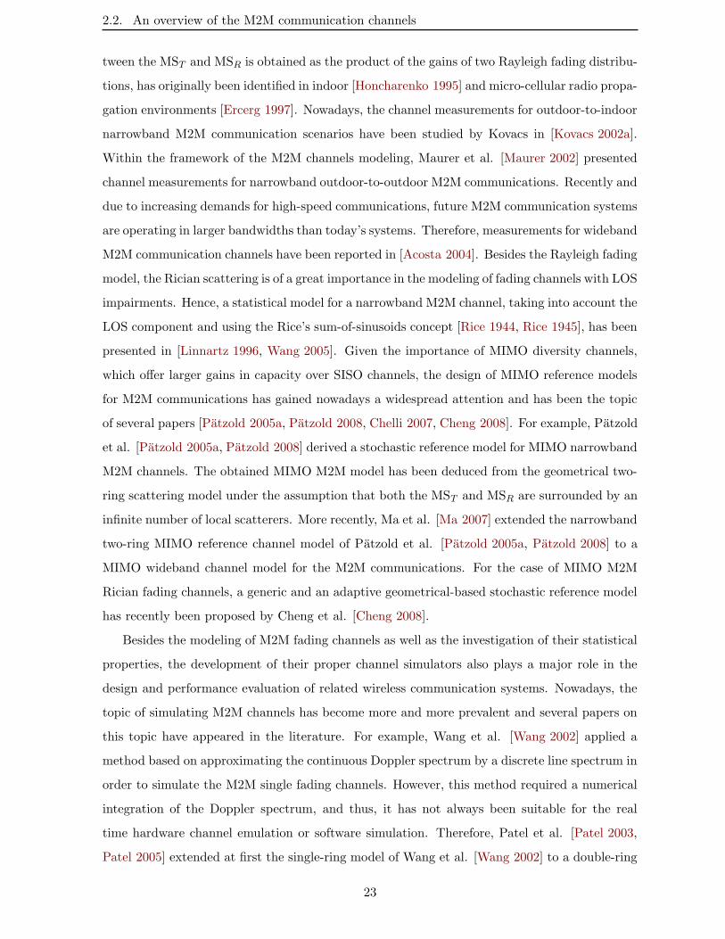
2.2. An overview of the M2M communication channels
tween the MST and MSR is obtained as the product of the gains of two Rayleigh fading distribu-
tions, has originally been identified in indoor [Honcharenko 1995] and micro-cellular radio propa-
gation environments [Ercerg 1997]. Nowadays, the channel measurements for outdoor-to-indoor
narrowband M2M communication scenarios have been studied by Kovacs in [Kovacs 2002a].
Within the framework of the M2M channels modeling, Maurer et al. [Maurer 2002] presented
channel measurements for narrowband outdoor-to-outdoor M2M communications. Recently and
due to increasing demands for high-speed communications, future M2M communication systems
are operating in larger bandwidths than today’s systems. Therefore, measurements for wideband
M2M communication channels have been reported in [Acosta 2004]. Besides the Rayleigh fading
model, the Rician scattering is of a great importance in the modeling of fading channels with LOS
impairments. Hence, a statistical model for a narrowband M2M channel, taking into account the
LOS component and using the Rice’s sum-of-sinusoids concept [Rice 1944, Rice 1945], has been
presented in [Linnartz 1996, Wang 2005]. Given the importance of MIMO diversity channels,
which offer larger gains in capacity over SISO channels, the design of MIMO reference models
for M2M communications has gained nowadays a widespread attention and has been the topic
of several papers [Patzold 2005a, Patzold 2008, Chelli 2007, Cheng 2008]. For example, Patzold
et al. [Patzold 2005a, Patzold 2008] derived a stochastic reference model for MIMO narrowband
M2M channels. The obtained MIMO M2M model has been deduced from the geometrical two-
ring scattering model under the assumption that both the MST and MSR are surrounded by an
infinite number of local scatterers. More recently, Ma et al. [Ma 2007] extended the narrowband
two-ring MIMO reference channel model of Patzold et al. [Patzold 2005a, Patzold 2008] to a
MIMO wideband channel model for the M2M communications. For the case of MIMO M2M
Rician fading channels, a generic and an adaptive geometrical-based stochastic reference model
has recently been proposed by Cheng et al. [Cheng 2008].
Besides the modeling of M2M fading channels as well as the investigation of their statistical
properties, the development of their proper channel simulators also plays a major role in the
design and performance evaluation of related wireless communication systems. Nowadays, the
topic of simulating M2M channels has become more and more prevalent and several papers on
this topic have appeared in the literature. For example, Wang et al. [Wang 2002] applied a
method based on approximating the continuous Doppler spectrum by a discrete line spectrum in
order to simulate the M2M single fading channels. However, this method required a numerical
integration of the Doppler spectrum, and thus, it has not always been suitable for the real
time hardware channel emulation or software simulation. Therefore, Patel et al. [Patel 2003,
Patel 2005] extended at first the single-ring model of Wang et al. [Wang 2002] to a double-ring
23
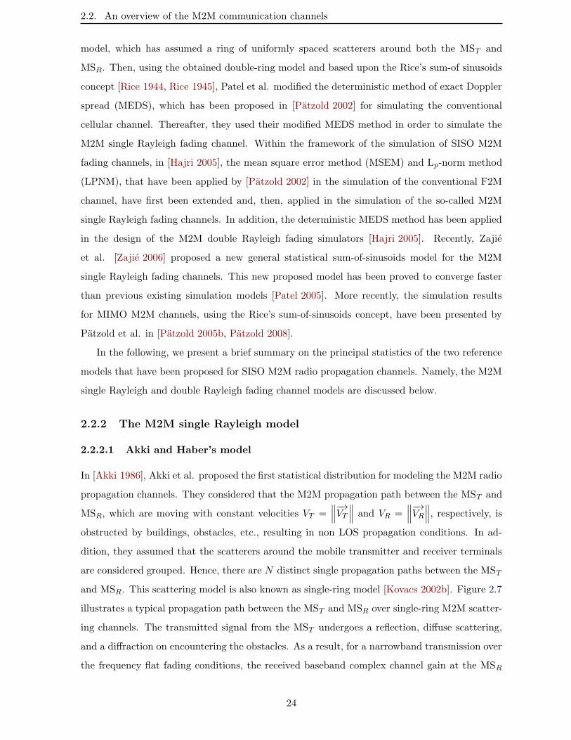
2.2. An overview of the M2M communication channels
model, which has assumed a ring of uniformly spaced scatterers around both the MST and
MSR. Then, using the obtained double-ring model and based upon the Rice’s sum-of sinusoids
concept [Rice 1944, Rice 1945], Patel et al. modified the deterministic method of exact Doppler
spread (MEDS), which has been proposed in [Patzold 2002] for simulating the conventional
cellular channel. Thereafter, they used their modified MEDS method in order to simulate the
M2M single Rayleigh fading channel. Within the framework of the simulation of SISO M2M
fading channels, in [Hajri 2005], the mean square error method (MSEM) and Lp-norm method
(LPNM), that have been applied by [Patzold 2002] in the simulation of the conventional F2M
channel, have first been extended and, then, applied in the simulation of the so-called M2M
single Rayleigh fading channels. In addition, the deterministic MEDS method has been applied
in the design of the M2M double Rayleigh fading simulators [Hajri 2005]. Recently, Zajie
et al. [Zajie 2006] proposed a new general statistical sum-of-sinusoids model for the M2M
single Rayleigh fading channels. This new proposed model has been proved to converge faster
than previous existing simulation models [Patel 2005]. More recently, the simulation results
for MIMO M2M channels, using the Rice’s sum-of-sinusoids concept, have been presented by
Patzold et al. in [Patzold 2005b, Patzold 2008].
In the following, we present a brief summary on the principal statistics of the two reference
models that have been proposed for SISO M2M radio propagation channels. Namely, the M2M
single Rayleigh and double Rayleigh fading channel models are discussed below.
2.2.2 The M2M single Rayleigh model
2.2.2.1 Akki and Haber’s model
In [Akki 1986], Akki et al. proposed the first statistical distribution for modeling the M2M radio
propagation channels. They considered that the M2M propagation path between the MST and
MSR, which are moving with constant velocities VT =∥∥∥−→VT
∥∥∥ and VR =∥∥∥−→VR
∥∥∥, respectively, is
obstructed by buildings, obstacles, etc., resulting in non LOS propagation conditions. In ad-
dition, they assumed that the scatterers around the mobile transmitter and receiver terminals
are considered grouped. Hence, there are N distinct single propagation paths between the MST
and MSR. This scattering model is also known as single-ring model [Kovacs 2002b]. Figure 2.7
illustrates a typical propagation path between the MST and MSR over single-ring M2M scatter-
ing channels. The transmitted signal from the MST undergoes a reflection, diffuse scattering,
and a diffraction on encountering the obstacles. As a result, for a narrowband transmission over
the frequency flat fading conditions, the received baseband complex channel gain at the MSR
24
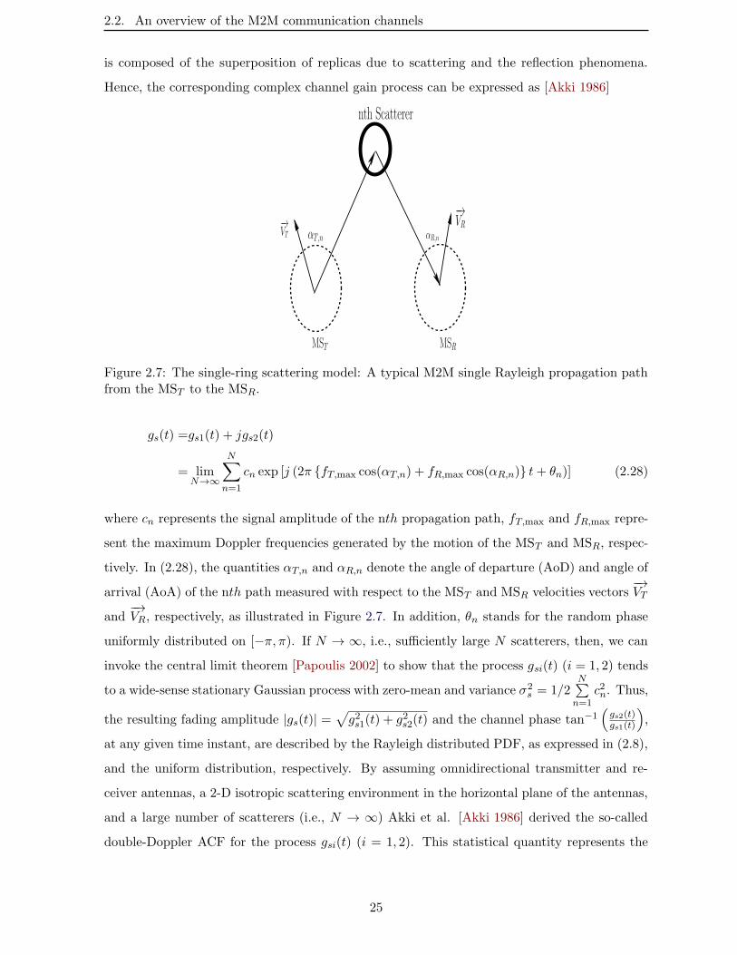
2.2. An overview of the M2M communication channels
is composed of the superposition of replicas due to scattering and the reflection phenomena.
Hence, the corresponding complex channel gain process can be expressed as [Akki 1986]
αR,n−→VT
−→VR
αT,n
MSRMST
nth Scatterer
Figure 2.7: The single-ring scattering model: A typical M2M single Rayleigh propagation pathfrom the MST to the MSR.
gs(t) =gs1(t) + jgs2(t)
= limN→∞
N∑
n=1
cn exp [j (2π fT,max cos(αT,n) + fR,max cos(αR,n) t+ θn)] (2.28)
where cn represents the signal amplitude of the nth propagation path, fT,max and fR,max repre-
sent the maximum Doppler frequencies generated by the motion of the MST and MSR, respec-
tively. In (2.28), the quantities αT,n and αR,n denote the angle of departure (AoD) and angle of
arrival (AoA) of the nth path measured with respect to the MST and MSR velocities vectors−→VT
and−→VR, respectively, as illustrated in Figure 2.7. In addition, θn stands for the random phase
uniformly distributed on [−π, π). If N → ∞, i.e., sufficiently large N scatterers, then, we can
invoke the central limit theorem [Papoulis 2002] to show that the process gsi(t) (i = 1, 2) tends
to a wide-sense stationary Gaussian process with zero-mean and variance σ2s = 1/2
N∑n=1
c2n. Thus,
the resulting fading amplitude |gs(t)| =√g2s1(t) + g2s2(t) and the channel phase tan−1
(gs2(t)gs1(t)
),
at any given time instant, are described by the Rayleigh distributed PDF, as expressed in (2.8),
and the uniform distribution, respectively. By assuming omnidirectional transmitter and re-
ceiver antennas, a 2-D isotropic scattering environment in the horizontal plane of the antennas,
and a large number of scatterers (i.e., N → ∞) Akki et al. [Akki 1986] derived the so-called
double-Doppler ACF for the process gsi(t) (i = 1, 2). This statistical quantity represents the
25
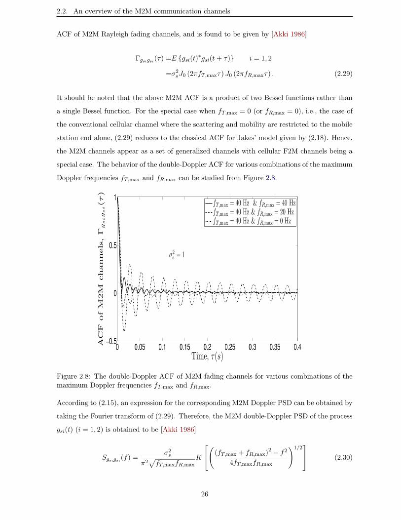
2.2. An overview of the M2M communication channels
ACF of M2M Rayleigh fading channels, and is found to be given by [Akki 1986]
Γgsigsi(τ) =E gsi(t)∗gsi(t+ τ) i = 1, 2
=σ2sJ0 (2πfT,maxτ) J0 (2πfR,maxτ) . (2.29)
It should be noted that the above M2M ACF is a product of two Bessel functions rather than
a single Bessel function. For the special case when fT,max = 0 (or fR,max = 0), i.e., the case of
the conventional cellular channel where the scattering and mobility are restricted to the mobile
station end alone, (2.29) reduces to the classical ACF for Jakes’ model given by (2.18). Hence,
the M2M channels appear as a set of generalized channels with cellular F2M channels being a
special case. The behavior of the double-Doppler ACF for various combinations of the maximum
Doppler frequencies fT,max and fR,max can be studied from Figure 2.8.
0 0.05 0.1 0.15 0.2 0.25 0.3 0.35 0.4−0.5
0
0.5
1
Time, τ(s)
AC
Fof
M2M
channels
,Γgsigsi(τ)
fT,max = 40 Hz & fR,max = 40 HzfT,max = 40 Hz & fR,max = 20 HzfT,max = 40 Hz & fR,max = 0 Hz
σ2s = 1
Figure 2.8: The double-Doppler ACF of M2M fading channels for various combinations of themaximum Doppler frequencies fT,max and fR,max.
According to (2.15), an expression for the corresponding M2M Doppler PSD can be obtained by
taking the Fourier transform of (2.29). Therefore, the M2M double-Doppler PSD of the process
gsi(t) (i = 1, 2) is obtained to be [Akki 1986]
Sgsigsi(f) =σ2s
π2√fT,maxfR,max
K
((fT,max + fR,max)
2 − f2
4fT,maxfR,max
)1/2 (2.30)
26
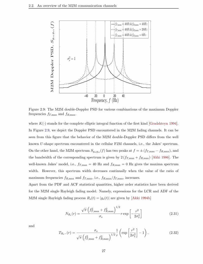
2.2. An overview of the M2M communication channels
−40 20 0 20 40Frequency, f (Hz)
M2M
Dopple
rP
SD
,Sgsigsi(f
)
fT,max = 40Hz&fR,max = 40Hz
fT,max = 40Hz&fR,max = 20Hz
fT,max = 40Hz&fR,max = 0Hz
σ2s = 1
Figure 2.9: The M2M double-Doppler PSD for various combinations of the maximum Dopplerfrequencies fT,max and fR,max.
where K(·) stands for the complete elliptic integral function of the first kind [Gradshteyn 1994].
In Figure 2.9, we depict the Doppler PSD encountered in the M2M fading channels. It can be
seen from this figure that the behavior of the M2M double-Doppler PSD differs from the well
known U -shape spectrum encountered in the cellular F2M channels, i.e., the Jakes’ spectrum.
On the other hand, the M2M spectrum Sgsigsi(f) has two peaks at f = ± (fT,max − fR,max), and
the bandwidth of the corresponding spectrum is given by 2 (fT,max + fR,max) [Akki 1986]. The
well-known Jakes’ model, i.e., fT,max = 40 Hz and fR,max = 0 Hz gives the maxima spectrum
width. However, this spectrum width decreases continually when the value of the ratio of
maximum frequencies fR,max and fT,max, i.e., fR,max/fT,max, increases.
Apart from the PDF and ACF statistical quantities, higher order statistics have been derived
for the M2M single Rayleigh fading model. Namely, expressions for the LCR and ADF of the
M2M single Rayleigh fading process Rs(t) = |gs(t)| are given by [Akki 1994b]
NRs(r) =
√π(f2T,max + f2R,max
)1/2
σsr exp
[− r2
2σ2s
](2.31)
and
TRs−(r) =σs
√π(f2T,max + f2R,max
)1/21
r
(exp
[r2
2σ2s
]− 1
), (2.32)
27
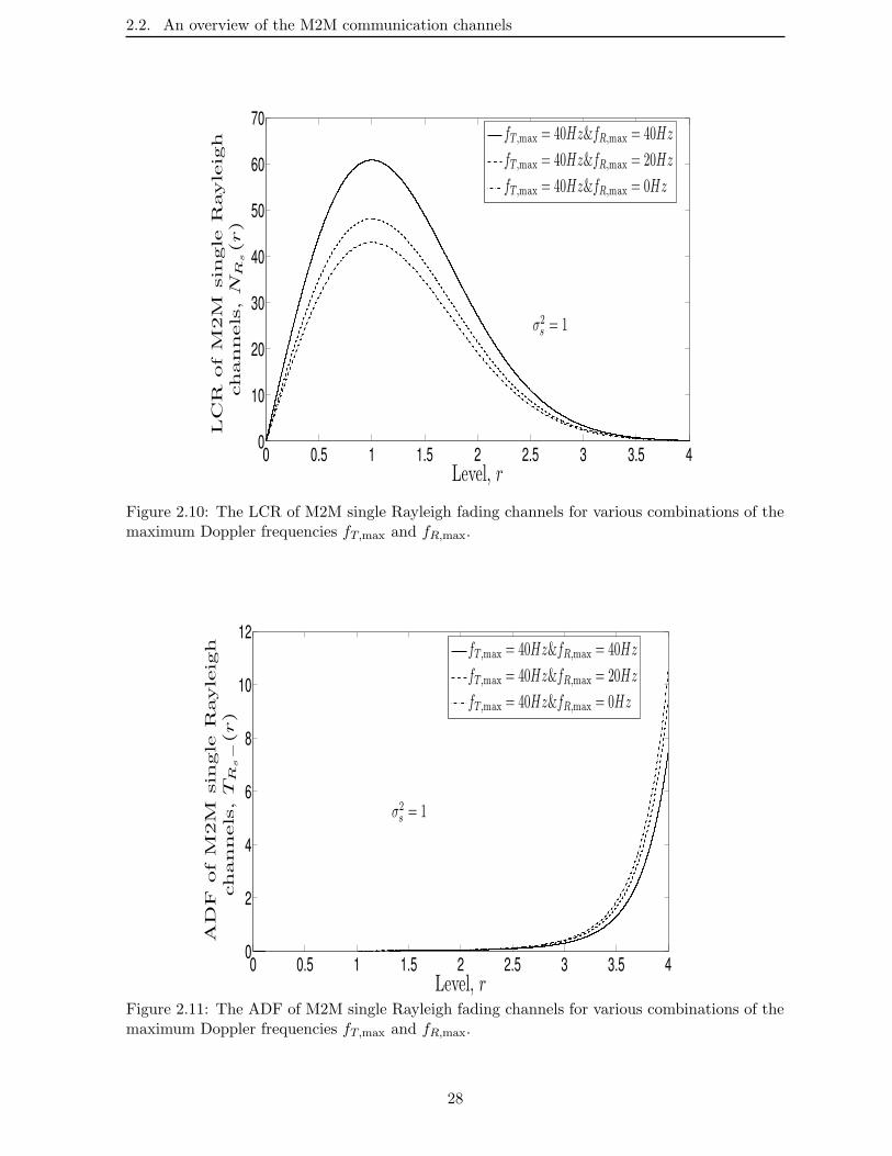
2.2. An overview of the M2M communication channels
0 0.5 1 1.5 2 2.5 3 3.5 40
10
20
30
40
50
60
70
Level, r
LC
Rof
M2M
sin
gle
Rayle
igh
channels
,NRs(r)
fT,max = 40Hz&fR,max = 40Hz
fT,max = 40Hz&fR,max = 20Hz
fT,max = 40Hz&fR,max = 0Hz
σ2s = 1
Figure 2.10: The LCR of M2M single Rayleigh fading channels for various combinations of themaximum Doppler frequencies fT,max and fR,max.
0 0.5 1 1.5 2 2.5 3 3.5 40
2
4
6
8
10
12
Level, r
AD
Fof
M2M
sin
gle
Rayle
igh
channels
,TRs−
(r)
fT,max = 40Hz&fR,max = 40Hz
fT,max = 40Hz&fR,max = 20Hz
fT,max = 40Hz&fR,max = 0Hz
σ2s = 1
Figure 2.11: The ADF of M2M single Rayleigh fading channels for various combinations of themaximum Doppler frequencies fT,max and fR,max.
28
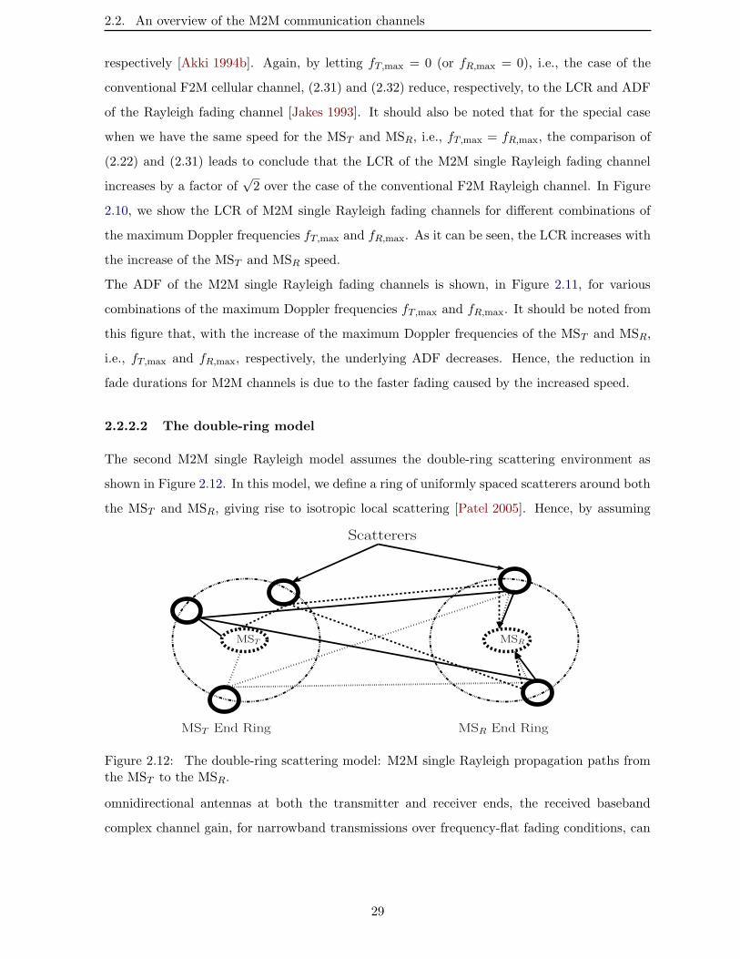
2.2. An overview of the M2M communication channels
respectively [Akki 1994b]. Again, by letting fT,max = 0 (or fR,max = 0), i.e., the case of the
conventional F2M cellular channel, (2.31) and (2.32) reduce, respectively, to the LCR and ADF
of the Rayleigh fading channel [Jakes 1993]. It should also be noted that for the special case
when we have the same speed for the MST and MSR, i.e., fT,max = fR,max, the comparison of
(2.22) and (2.31) leads to conclude that the LCR of the M2M single Rayleigh fading channel
increases by a factor of√2 over the case of the conventional F2M Rayleigh channel. In Figure
2.10, we show the LCR of M2M single Rayleigh fading channels for different combinations of
the maximum Doppler frequencies fT,max and fR,max. As it can be seen, the LCR increases with
the increase of the MST and MSR speed.
The ADF of the M2M single Rayleigh fading channels is shown, in Figure 2.11, for various
combinations of the maximum Doppler frequencies fT,max and fR,max. It should be noted from
this figure that, with the increase of the maximum Doppler frequencies of the MST and MSR,
i.e., fT,max and fR,max, respectively, the underlying ADF decreases. Hence, the reduction in
fade durations for M2M channels is due to the faster fading caused by the increased speed.
2.2.2.2 The double-ring model
The second M2M single Rayleigh model assumes the double-ring scattering environment as
shown in Figure 2.12. In this model, we define a ring of uniformly spaced scatterers around both
the MST and MSR, giving rise to isotropic local scattering [Patel 2005]. Hence, by assuming
Scatterers
MST End Ring MSR End Ring
MSRMST
Figure 2.12: The double-ring scattering model: M2M single Rayleigh propagation paths fromthe MST to the MSR.
omnidirectional antennas at both the transmitter and receiver ends, the received baseband
complex channel gain, for narrowband transmissions over frequency-flat fading conditions, can
29
2.2. An overview of the M2M communication channels
be written as [Patel 2005]
gd(t) = limM,N→∞
M∑
k=1
N∑
n=1
ckn exp [j (2π fT,max cos(αT,k) + fR,max cos(αR,n) t+ θkn)] (2.33)
where the index k refers to the paths traveling from the MST to theM scatterers located on the
MSR end ring, while the index n refers to the paths traveling from the MSR to the N scatterers
located on the MST end ring. In (2.33), ckn and θkn denote the joint amplitude and joint phase
caused by the interaction of the M transmitter and N receiver scatterers.
The above double-ring scattering model appears as a more generic M2M model than the last
single-ring model [Patel 2005]. However, all its statistical quantities, e.g., the PDF, ACF,
Doppler PSD, etc., have been demonstrated to be the same as that already derived for the
single-ring scattering model. Therefore, when an isotropic scattering is assumed, the double-
ring model corresponds to the M2M single Rayleigh model.
2.2.3 The double Rayleigh model
2.2.3.1 The general double-ring model
The general double-ring model also known as the so-called cascaded or double Rayleigh model
has been presented in [Kovacs 2002a, Kovacs 2002b]. This model assumes the double-ring scat-
tering propagation environment as shown in Figure 2.12. However, in the corresponding prop-
agation scenario, we assume that the distance between the MST and MSR is considered to be
large. In this case, the complex received channel gain signal can be described by the product
of two complex Gaussian processes according to [Kovacs 2002a, Kovacs 2002b]
gD(t) = limM→∞
M∑
k=1
Ak exp [j (2πfT,max cos(αT,k)t+ θT,k)]
× limN→∞
N∑
n=1
Bn exp [j (2πfR,max cos(αR,n)t+ θR,n)] (2.34)
where Ak, θT,k, Bn, and θR,n are independently distributed random amplitudes and phases due
to local scatterers around the MST and MSR, respectively. The expression (2.34) can also be
expressed as
gD(t) =gD1(t)× gD2
(t) (2.35)
30
2.2. An overview of the M2M communication channels
where gD1(t) and gD1
(t) are given by
gD1(t) = lim
M→∞
M∑
k=1
Ak exp [j (2πfT,max cos(αT,k)t+ θT,k)] (2.36)
and
gD2(t) = lim
N→∞
N∑
n=1
Bn exp [j (2πfR,max cos(αR,n)t+ θR,n)], (2.37)
respectively. It should be noted that (2.35) is more generic than (2.33) because the signal ampli-
tudes corresponding to the propagation paths are considered as independent random variables
and not as a product of independent uniformly distributed random variables. The fading process
of the corresponding fading channel is given by RD(t) = |gD(t)|. By introducing the quantities
RD1(t) = |gD1
(t)| and RD2(t) = |gD2
(t)|, the process RD(t) can be written as
RD(t) = RD1(t)RD2
(t). (2.38)
The process RD(t) is generally known as the double Rayleigh fading amplitude which corre-
sponds to that of the product of the two independent Rayleigh processes RD1(t) and RD2
(t).
An analytical expression for the PDF of the double Rayleigh process RD(t), which is known
as the double Rayleigh distribution, has been derived in [Kovacs 2002a, Kovacs 2002b] and has
the form
pRD(z) =
z
σ2D1σ2D2
K0
(z
σD1σD2
)(2.39)
where K0(·) is the zeroth order modified Bessel function of the second kind [Gradshteyn 1994].
Also in (2.39), σ2D1and σ2D2
stand for the mean powers of the two independent Rayleigh processes
RD1(t) and RD2
(t), respectively. In Figure 2.13, we show the behavior of the amplitude PDF,
pRD(z), of the M2M double Rayleigh model for various combinations of the mean powers σ2
D1
and σ2D2. It should be noted from this figure that for the same mean powers values σ2
D1and
σ2D2, i.e., σ2D1
= σ2D1, the PDF maxima and the PDF spread increase with the decrease and
the increase of the mean power values σ2D1
and σ2D1(σ2D1
= σ2D1), respectively. The ACF of
the double Rayleigh model, i.e., the model described by the process gD(t), is also given by the
so-called double-Doppler ACF expressed by (2.29) [Akki 1986].
31
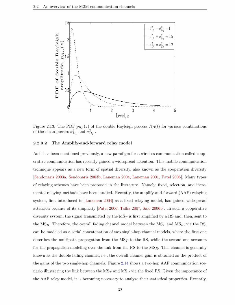
2.2. An overview of the M2M communication channels
0 1 2 3 4 50
0.5
1
1.5
2
2.5
Level, z
PD
Fof
double
Rayle
igh
am
plitude,pRD
(z)
σ2D1
= σ2D2
= 1
σ2D1
= σ2D2
= 0.5
σ2D1
= σ2D2
= 0.2
Figure 2.13: The PDF pRD(z) of the double Rayleigh process RD(t) for various combinations
of the mean powers σ2D1and σ2D2
.
2.2.3.2 The Amplify-and-forward relay model
As it has been mentioned previously, a new paradigm for a wireless communication called coop-
erative communication has recently gained a widespread attention. This mobile communication
technique appears as a new form of spatial diversity, also known as the cooperation diversity
[Sendonaris 2003a, Sendonaris 2003b, Laneman 2004, Laneman 2001, Patel 2006]. Many types
of relaying schemes have been proposed in the literature. Namely, fixed, selection, and incre-
mental relaying methods have been studied. Recently, the amplify-and-forward (AAF) relaying
system, first introduced in [Laneman 2004] as a fixed relaying model, has gained widespread
attention because of its simplicity [Patel 2006, Talha 2007, Salo 2006b]. In such a cooperative
diversity system, the signal transmitted by the MST is first amplified by a RS and, then, sent to
the MSR. Therefore, the overall fading channel model between the MST and MSR, via the RS,
can be modeled as a serial concatenation of two single-hop channel models, where the first one
describes the multipath propagation from the MST to the RS, while the second one accounts
for the propagation modeling over the link from the RS to the MSR. This channel is generally
known as the double fading channel, i.e., the overall channel gain is obtained as the product of
the gains of the two single-hop channels. Figure 2.14 shows a two-hop AAF communication sce-
nario illustrating the link between the MST and MSR via the fixed RS. Given the importance of
the AAF relay model, it is becoming necessary to analyze their statistical properties. Recently,
32
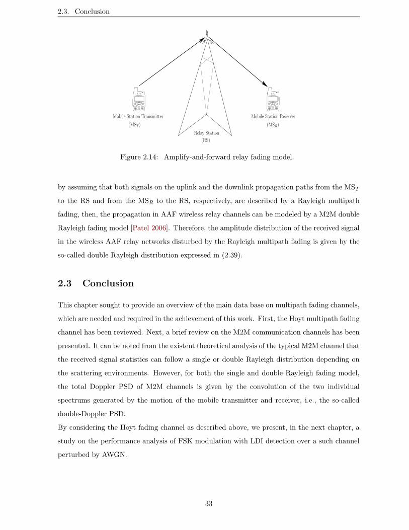
2.3. Conclusion
(RS)
Mobile Station ReceiverMobile Station Transmitter
(MST ) (MSR)
Relay Station
Figure 2.14: Amplify-and-forward relay fading model.
by assuming that both signals on the uplink and the downlink propagation paths from the MST
to the RS and from the MSR to the RS, respectively, are described by a Rayleigh multipath
fading, then, the propagation in AAF wireless relay channels can be modeled by a M2M double
Rayleigh fading model [Patel 2006]. Therefore, the amplitude distribution of the received signal
in the wireless AAF relay networks disturbed by the Rayleigh multipath fading is given by the
so-called double Rayleigh distribution expressed in (2.39).
2.3 Conclusion
This chapter sought to provide an overview of the main data base on multipath fading channels,
which are needed and required in the achievement of this work. First, the Hoyt multipath fading
channel has been reviewed. Next, a brief review on the M2M communication channels has been
presented. It can be noted from the existent theoretical analysis of the typical M2M channel that
the received signal statistics can follow a single or double Rayleigh distribution depending on
the scattering environments. However, for both the single and double Rayleigh fading model,
the total Doppler PSD of M2M channels is given by the convolution of the two individual
spectrums generated by the motion of the mobile transmitter and receiver, i.e., the so-called
double-Doppler PSD.
By considering the Hoyt fading channel as described above, we present, in the next chapter, a
study on the performance analysis of FSK modulation with LDI detection over a such channel
perturbed by AWGN.
33
Chapter 3
BEP of FSK with LDI detection
over Hoyt fading channels
The investigation of the error rate performance of the FSK modulation with an LDI detection
has been widely studied for the case of the Rayleigh and Rice fading channels [Tjhung 1990,
Ng 1994, Korn 1990a, Korn 1990b]. In [Tjhung 1990, Ng 1994], closed-form expressions for the
BEP performance have been reported for a transmission over Rayleigh fading and the validity
of the results has been verified by using experimental data. For the Rice fading model, the error
analysis of M -FSK transmission has been studied in [Korn 1990a, Korn 1990b]. By considering
the Hoyt fading channel, a closed-form expression for the BEP of FSK modulation with the
classical limiter discriminator (LD) detection has been derived [Zhaounia 2004]. In this study,
a rectangular shape for the predetection filter has been used and no integrate and dump filter
has been assumed (sampling discriminator),
In this chapter, we present a performance analysis of a narrowband digital FSK modulation
scheme with an LDI detection over the Hoyt mobile fading channels. First, we derive a closed-
form expression for the PDF of the phase angle between two Hoyt fading vectors. Then, an
expression for the PDF of the phase noise due to additive Gaussian noise, is presented. The
average number of FM clicks occurring at the output of a digital FM receiver is expressed, in
Section 3.4. Based on the theory of the BEP performance and all the underlying investigated
quantities, a formula for the BEP performance of FSK with LDI detection scheme operating
over Hoyt mobile fading channels is obtained. Then, we present numerical examples to illustrate
the analysis and study the influence of the fading severity as well as the FM system parameters
on the obtained BEP performance. Finally, Section 3.7 concludes the chapter.
3.1 FSK system model
The binary FSK system with an LDI detection under study is depicted, as a block diagram,
in Figure 3.1. The transmitted FSK signal st(t) can be expressed, in the equivalent complex
34
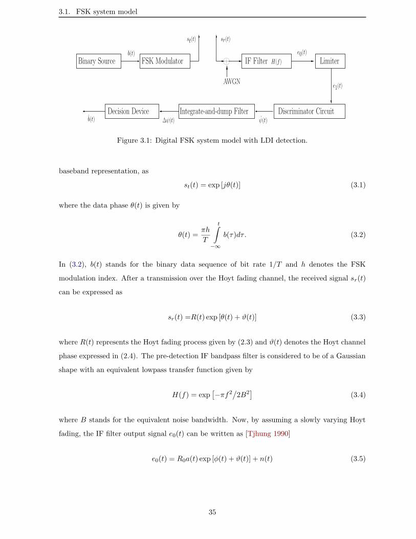
3.1. FSK system model
b(t)
IF Filter H(f ) Limiter
Discriminator CircuitDecision Device Integrate-and-dump Filter
Binary Source FSK Modulator
∆ψ(t) ψ(t)
AWGN
e0(t)
e1(t)
b(t)
st(t) sr(t)
Figure 3.1: Digital FSK system model with LDI detection.
baseband representation, as
st(t) = exp [jθ(t)] (3.1)
where the data phase θ(t) is given by
θ(t) =πh
T
t∫
−∞
b(τ)dτ . (3.2)
In (3.2), b(t) stands for the binary data sequence of bit rate 1/T and h denotes the FSK
modulation index. After a transmission over the Hoyt fading channel, the received signal sr(t)
can be expressed as
sr(t) =R(t) exp [θ(t) + ϑ(t)] (3.3)
where R(t) represents the Hoyt fading process given by (2.3) and ϑ(t) denotes the Hoyt channel
phase expressed in (2.4). The pre-detection IF bandpass filter is considered to be of a Gaussian
shape with an equivalent lowpass transfer function given by
H(f) = exp[−πf2
/2B2
](3.4)
where B stands for the equivalent noise bandwidth. Now, by assuming a slowly varying Hoyt
fading, the IF filter output signal e0(t) can be written as [Tjhung 1990]
e0(t) = R0a(t) exp [φ(t) + ϑ(t)] + n(t) (3.5)
35
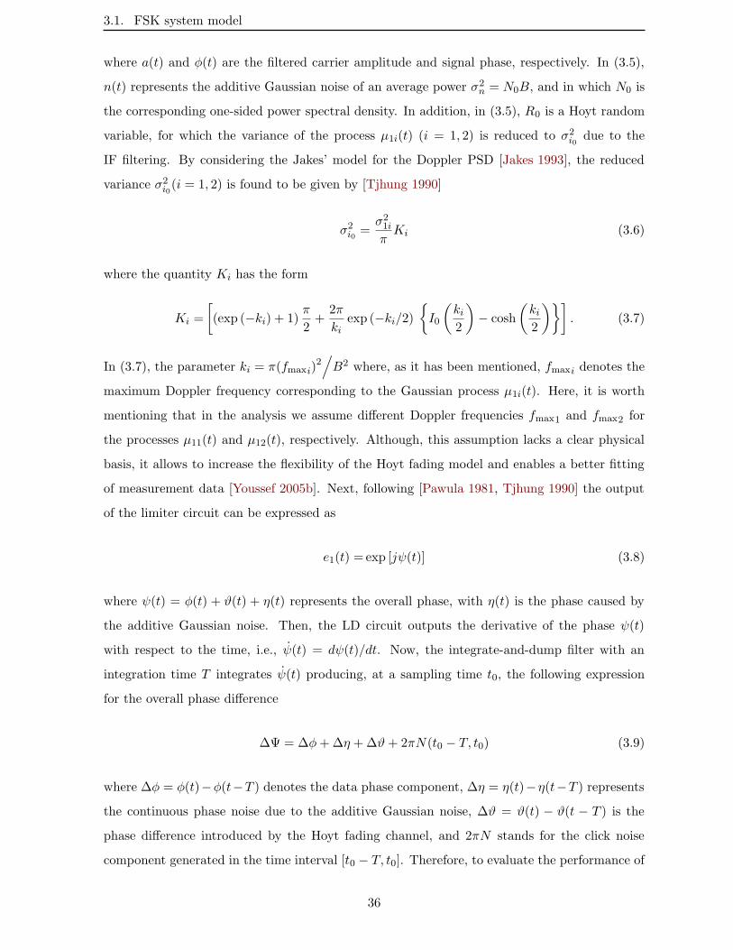
3.1. FSK system model
where a(t) and φ(t) are the filtered carrier amplitude and signal phase, respectively. In (3.5),
n(t) represents the additive Gaussian noise of an average power σ2n = N0B, and in which N0 is
the corresponding one-sided power spectral density. In addition, in (3.5), R0 is a Hoyt random
variable, for which the variance of the process µ1i(t) (i = 1, 2) is reduced to σ2i0 due to the
IF filtering. By considering the Jakes’ model for the Doppler PSD [Jakes 1993], the reduced
variance σ2i0(i = 1, 2) is found to be given by [Tjhung 1990]
σ2i0 =σ21iπKi (3.6)
where the quantity Ki has the form
Ki =
[(exp (−ki) + 1)
π
2+
2π
kiexp (−ki/2)
I0
(ki2
)− cosh
(ki2
)]. (3.7)
In (3.7), the parameter ki = π(fmaxi)2/B2 where, as it has been mentioned, fmaxi denotes the
maximum Doppler frequency corresponding to the Gaussian process µ1i(t). Here, it is worth
mentioning that in the analysis we assume different Doppler frequencies fmax1 and fmax2 for
the processes µ11(t) and µ12(t), respectively. Although, this assumption lacks a clear physical
basis, it allows to increase the flexibility of the Hoyt fading model and enables a better fitting
of measurement data [Youssef 2005b]. Next, following [Pawula 1981, Tjhung 1990] the output
of the limiter circuit can be expressed as
e1(t) = exp [jψ(t)] (3.8)
where ψ(t) = φ(t) + ϑ(t) + η(t) represents the overall phase, with η(t) is the phase caused by
the additive Gaussian noise. Then, the LD circuit outputs the derivative of the phase ψ(t)
with respect to the time, i.e., ψ(t) = dψ(t)/dt. Now, the integrate-and-dump filter with an
integration time T integrates ψ(t) producing, at a sampling time t0, the following expression
for the overall phase difference
∆Ψ = ∆φ+∆η +∆ϑ+ 2πN(t0 − T, t0) (3.9)
where ∆φ = φ(t)−φ(t−T ) denotes the data phase component, ∆η = η(t)−η(t−T ) representsthe continuous phase noise due to the additive Gaussian noise, ∆ϑ = ϑ(t) − ϑ(t − T ) is the
phase difference introduced by the Hoyt fading channel, and 2πN stands for the click noise
component generated in the time interval [t0 − T, t0]. Therefore, to evaluate the performance of
36
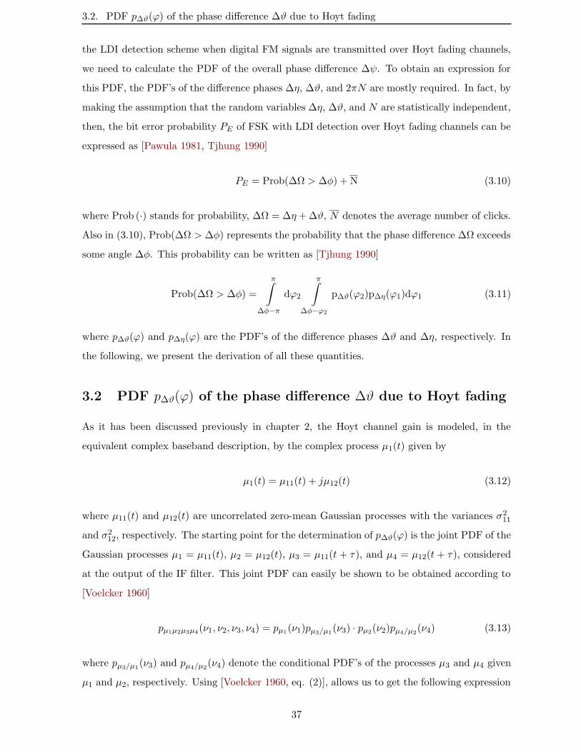
3.2. PDF p∆ϑ(ϕ) of the phase difference ∆ϑ due to Hoyt fading
the LDI detection scheme when digital FM signals are transmitted over Hoyt fading channels,
we need to calculate the PDF of the overall phase difference ∆ψ. To obtain an expression for
this PDF, the PDF’s of the difference phases ∆η, ∆ϑ, and 2πN are mostly required. In fact, by
making the assumption that the random variables ∆η, ∆ϑ, and N are statistically independent,
then, the bit error probability PE of FSK with LDI detection over Hoyt fading channels can be
expressed as [Pawula 1981, Tjhung 1990]
PE = Prob(∆Ω > ∆φ) + N (3.10)
where Prob (·) stands for probability, ∆Ω = ∆η+∆ϑ, N denotes the average number of clicks.
Also in (3.10), Prob(∆Ω > ∆φ) represents the probability that the phase difference ∆Ω exceeds
some angle ∆φ. This probability can be written as [Tjhung 1990]
Prob(∆Ω > ∆φ) =
π∫
∆φ−π
dϕ2
π∫
∆φ−ϕ2
p∆ϑ(ϕ2)p∆η(ϕ1)dϕ1 (3.11)
where p∆ϑ(ϕ) and p∆η(ϕ) are the PDF’s of the difference phases ∆ϑ and ∆η, respectively. In
the following, we present the derivation of all these quantities.
3.2 PDF p∆ϑ(ϕ) of the phase difference ∆ϑ due to Hoyt fading
As it has been discussed previously in chapter 2, the Hoyt channel gain is modeled, in the
equivalent complex baseband description, by the complex process µ1(t) given by
µ1(t) = µ11(t) + jµ12(t) (3.12)
where µ11(t) and µ12(t) are uncorrelated zero-mean Gaussian processes with the variances σ211
and σ212, respectively. The starting point for the determination of p∆ϑ(ϕ) is the joint PDF of the
Gaussian processes µ1 = µ11(t), µ2 = µ12(t), µ3 = µ11(t + τ), and µ4 = µ12(t + τ), considered
at the output of the IF filter. This joint PDF can easily be shown to be obtained according to
[Voelcker 1960]
pµ1µ2µ3µ4(ν1, ν2, ν3, ν4) = pµ1(ν1)pµ3/µ1(ν3) · pµ2(ν2)pµ4/µ2(ν4) (3.13)
where pµ3/µ1(ν3) and pµ4/µ2(ν4) denote the conditional PDF’s of the processes µ3 and µ4 given
µ1 and µ2, respectively. Using [Voelcker 1960, eq. (2)], allows us to get the following expression
37
3.2. PDF p∆ϑ(ϕ) of the phase difference ∆ϑ due to Hoyt fading
for the joint PDF pµ1µ2µ3µ4(ν1, ν2, ν3, ν4)
pµ1µ2µ3µ4(ν1, ν2, ν3, ν4) =A1 exp[−A2
σ220κν
21 + σ210λν
22 + σ220κν
23 + σ210λν
24 (3.14)
− 2(σ220κρτ1ν1ν3 + σ210λρτ2ν2ν4
)]
where ρτi (i = 1, 2) is the normalized ACF of the process µ1i(t) and the quantities λ, κ, A1,
and A2 are, respectively, given by
λ =1− ρ2τ1
κ =1− ρ2τ2
A1 =1
4π2σ210σ220
√λκ
A2 =1
2σ210σ220λκ. (3.15)
Now, by making use of the variable transformation given by
µ1 = R1 cosϑ1
µ2 = R1 sinϑ1
µ3 = R2 cosϑ2
µ4 = R2 sinϑ2(3.16)
we obtain the following expression for the joint PDF pR1R2ϑ1ϑ2(z1, z2, ϕ1, ϕ2) of the variables
R1, R2, ϑ1, and ϑ2
pR1R2ϑ1ϑ2(z1, z2, ϕ1, ϕ2) =A1z1z2 exp[−A2
z21(σ220κ cos
2 ϕ1 +σ210λ sin2 ϕ1
)
+ z22(σ220κ cos
2 ϕ2 + σ210λ sin2 ϕ2
)− 2z1z2
(σ220κρτ1 cosϕ1 cosϕ2
+ σ210λρτ2 sinϕ1 sinϕ2
)](3.17)
where 0 ≤ z1, z2 < ∞ and −π ≤ ϕ1, ϕ2 < π. Therefore, the joint PDF pϑ1ϑ2(ϕ1, ϕ2) of the
phases ϑ1 and ϑ2 can be computed according to
pϑ1ϑ2(ϕ1, ϕ2) =
∞∫
0
∞∫
0
pR1R2ϑ1ϑ2(z1, z2, ϕ1, ϕ2)dz1dz2. (3.18)
The integrals involved in (3.18) can be solved analytically by making use of the multiple integrals
evaluation approach reported in [Rice 1944, Rice 1945]. Based on that approach, we start by
38
3.2. PDF p∆ϑ(ϕ) of the phase difference ∆ϑ due to Hoyt fading
considering the integral I given by
I =
∞∫
0
∞∫
0
exp[−A2σ
210Ez
21 −A2σ
210Fz
22 +2A2σ
210Dz1z2
]dz1dz2 (3.19)
where the quantities E, F , and D are expressed by
E =q20κ cos2 ϕ1 + λ sin2 ϕ1
F =q20κ cos2 θ2 + λ sin2 ϕ2
D =q20κρτ1 cosϕ1 cosϕ2 + λρτ2 sinϕ1 sinϕ2 (3.20)
and in which, the quantity q0 represents the reduced Hoyt fading parameter given by
q0 =σ20σ10
= q · K2
K1. (3.21)
In (3.21), q stands for the Hoyt fading parameter defined by (2.6). It should be mentioned that
for the special case corresponding to fmax1 = fmax2 , we have K1 = K2 and therefore q0 = q.
To solve the integrals in (3.19), we first let x1 = z1σ10 (A2E)1/2 and x2 = z2σ10 (A2F )1/2. This
leads to
I =1
A2σ210 (EF )1/2
∞∫
0
∞∫
0
exp[−x21 − x22 + 2gx1x2
]dx1dx2 (3.22)
where the parameter g = D
(EF )1/2. Then, we make the following linear change of variables
x1 = y1 + g(1− g2
)−1/2y2
x2 =(1− g2
)−1/2y2
(3.23)
which results in
− x21 − x22 + 2gx1x2 = −y21 − y22. (3.24)
Therefore, by applying these transformations, the integral I can be written as
I =
(1− g2
)−1/2
A2σ210 (EF )1/2
∞∫
0
dy2
∞∫
−g(1−g2)−1/2y2
exp[−y21 − y22
]dy1. (3.25)
39
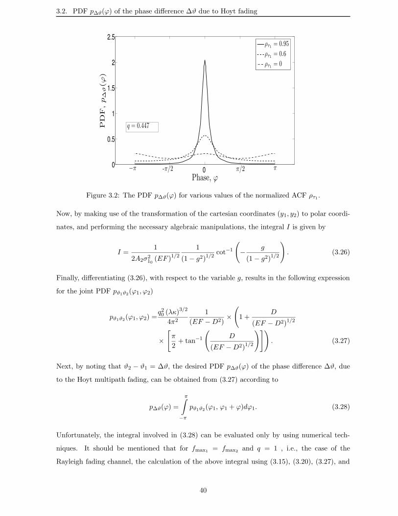
3.2. PDF p∆ϑ(ϕ) of the phase difference ∆ϑ due to Hoyt fading
0 0
0.5
1
1.5
2
2.5
Phase, ϕ
PD
F,p
∆ϑ(ϕ
)
ρτ1 = 0.95
ρτ1 = 0.6
ρτ1 = 0
q = 0.447
−π -π/2 π/2 π
Figure 3.2: The PDF p∆ϑ(ϕ) for various values of the normalized ACF ρτ1 .
Now, by making use of the transformation of the cartesian coordinates (y1, y2) to polar coordi-
nates, and performing the necessary algebraic manipulations, the integral I is given by
I =1
2A2σ210 (EF )1/2
1
(1− g2)1/2cot−1
(− g
(1− g2)1/2
). (3.26)
Finally, differentiating (3.26), with respect to the variable g, results in the following expression
for the joint PDF pϑ1ϑ2(ϕ1, ϕ2)
pϑ1ϑ2(ϕ1, ϕ2) =q20 (λκ)
3/2
4π21
(EF −D2)×(1 +
D
(EF −D2)1/2
×[π
2+ tan−1
(D
(EF −D2)1/2
)]). (3.27)
Next, by noting that ϑ2 − ϑ1 = ∆ϑ, the desired PDF p∆ϑ(ϕ) of the phase difference ∆ϑ, due
to the Hoyt multipath fading, can be obtained from (3.27) according to
p∆ϑ(ϕ) =
π∫
−π
pϑ1ϑ2(ϕ1, ϕ1 + ϕ)dϕ1. (3.28)
Unfortunately, the integral involved in (3.28) can be evaluated only by using numerical tech-
niques. It should be mentioned that for fmax1 = fmax2 and q = 1 , i.e., the case of the
Rayleigh fading channel, the calculation of the above integral using (3.15), (3.20), (3.27), and
40
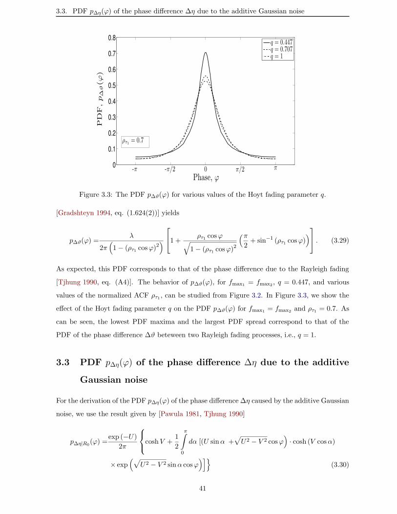
3.3. PDF p∆η(ϕ) of the phase difference ∆η due to the additive Gaussian noise
0
0.1
0.2
0.3
0.4
0.5
0.6
0.7
0.8
Phase, ϕ
PD
F,p
∆ϑ(ϕ
)
q = 0.447q = 0.707q = 1
-π π-π/2 π/20
ρτ1 = 0.7
Figure 3.3: The PDF p∆ϑ(ϕ) for various values of the Hoyt fading parameter q.
[Gradshteyn 1994, eq. (1.624(2))] yields
p∆ϑ(ϕ) =λ
2π(1− (ρτ1 cosϕ)
2)
1 + ρτ1 cosϕ√
1− (ρτ1 cosϕ)2
(π2+ sin−1 (ρτ1 cosϕ)
) . (3.29)
As expected, this PDF corresponds to that of the phase difference due to the Rayleigh fading
[Tjhung 1990, eq. (A4)]. The behavior of p∆ϑ(ϕ), for fmax1 = fmax2 , q = 0.447, and various
values of the normalized ACF ρτ1 , can be studied from Figure 3.2. In Figure 3.3, we show the
effect of the Hoyt fading parameter q on the PDF p∆ϑ(ϕ) for fmax1 = fmax2 and ρτ1 = 0.7. As
can be seen, the lowest PDF maxima and the largest PDF spread correspond to that of the
PDF of the phase difference ∆ϑ beteween two Rayleigh fading processes, i.e., q = 1.
3.3 PDF p∆η(ϕ) of the phase difference ∆η due to the additive
Gaussian noise
For the derivation of the PDF p∆η(ϕ) of the phase difference ∆η caused by the additive Gaussian
noise, we use the result given by [Pawula 1981, Tjhung 1990]
p∆η|R0(ϕ) =
exp (−U)
2π
coshV +
1
2
π∫
0
dα [(U sinα +√U2 − V 2 cosϕ
)· cosh (V cosα)
× exp(√
U2 − V 2 sinα cosϕ)]
(3.30)
41
3.3. PDF p∆η(ϕ) of the phase difference ∆η due to the additive Gaussian noise
which represents the conditional PDF of the phase difference ∆η given the reduced Hoyt random
variable R0. In (3.30), the quantities U and V are obtained to be
U =1
2[γ(t0) + γ(t0 − T )] =
R20
2σ2nC1
V =1
2[γ(t0)− γ(t0 − T )] =
R20
2σ2nC2. (3.31)
where the parameters C1 and C2 are functions of the specific bit patterns to be considered in
the evaluation of the BEP performance. Expressions for these parameters can be found in the
Appendix A. Also, in (3.31) the quantity γ(t) is the time varying SNR defined by
γ(t) =R2
0
2
a2(t)
σ2n=EbN0
1
BT
R20a
2(t)
(q2 + 1)σ211(3.32)
where Eb =(q2+1)
2 σ211T is the average received signal-energy-per-bit at the input of the IF filter.
Then, the desired quantity for p∆η(ϕ) can be obtained by averaging p∆η|R0(ϕ) over the reduced
Hoyt random variable R0 according to
p∆η(ϕ) =
∞∫
0
p∆η|R0(ϕ)pR0
(z)dz. (3.33)
Using [Gradshteyn 1994, Eqs. 6.611(1), 6.623(2), and 8.406(3)], the PDF p∆η(ϕ) can be written
as
p∆η(ϕ) =d
1√
[(C1 − C2) + e]2 − l2+
1√[(C1 + C2) + e]2 − l2
+d
2
π∫
0
dα (C1 sinα+ C3 cosϕ)
×
e− (C3 sinα cosϕ+ C2 cosα− C1)[e− (C3 sinα cosϕ+ C2 cosα− C1)]
2 − l23/2
+e− (C3 sinα cosϕ− C2 cosα− C1)
[e− (C3 sinα cosϕ− C2 cosα− C1)]2 − l2
3/2
(3.34)
42
3.4. Average number of FM clicks N
where the quantities C3, d, e, and l are given by
C3 =√C21 − C2
2
d =1 + q208π√q20r
e =
(1 + q20
)2
4q20r
l =1− q404q20
r. (3.35)
In (3.35), r = 2σ2n
(1+q20)σ2
10
. Unfortunately, the integral in (3.34) is difficult to handle, and it can
be evaluated only by using numerical techniques.
3.4 Average number of FM clicks N
Based on the assumption that the FM clicks, at the output of the discriminator circuit, can
be described statistically by a Poisson distributed discrete random variable [Rice 1963], the
average number of clicks N occurring during the time interval [t0 − T, t0], corresponding to the
bit duration T , can be derived according to the following relation [Pawula 1981, Tjhung 1990]
N =1
2π
∞∫
0
t0∫
t0−T
φ(τ) exp
(−z
2
2
a2(τ)
σ2n
)pR0
(z)dτdz. (3.36)
After some algebraic manipulations, we obtain the following quantity for the desired N
N = 2d
t0∫
t0−T
φ(τ)√[(a2(τ) + e)2 − l2
]dτ. (3.37)
For the special case corresponding to fmax1 = fmax2 and q = 1, (3.37) simplifies to the result
given by
N =σ2n
2πσ210
t0∫
t0−T
φ(τ)
a2(τ) + σ2n
σ2
10
dτ. (3.38)
As expected, this quantity corresponds perfectly to the average number of FM clicks, taking
into account the Rayleigh mutipath fading effects, that has been derived in [Tjhung 1990].
To summarize, the quantity given by (3.10), i.e., the BEP performance of the FSK with an LDI
detection over Hoyt fading channels, can be evaluated using (3.11), (3.28), (3.34), and (3.37).
43
3.5. Bit error rate probability
3.5 Bit error rate probability
According to [Pawula 1981, Tjhung 1990], for BT ≥ 1, the distortion caused by the intersymbol
interference (ISI), which are due to the bandwidth limitation of the pre-detetion bandpass IF
filter, extends only to one bit either side of the bit under detection. Thus, if we consider that
a ”1” bit is sent, the four bit patterns of “010”, “111”, “011”, and “110” will intervene in the
calculation of the desired average BEP. By symmetry, “011” and “110” can be considered to
have the same ISI effects upon the central bit. Therefore, only the three bit patterns given by
“010”, “111”, and “011”, will be considered in the calculation of the desired BEP perfromance.
For these three bit patterns, (3.10) can be approximated by [Tjhung 1990]
PE ∼= Pe,1 + Pe,2 (3.39)
where
Pe,1 =1
4[Prob (∆Ω > ∆φ |111 ) + Prob (∆Ω > ∆φ |010 ) + 2Prob (∆Ω > ∆φ |011 )] (3.40)
and
Pe,2 =1
4
[N |111 +N
∣∣010 + 2N |011
]. (3.41)
In (3.40), Prob (∆Ω > ∆φ |... ) represents the conditional error probability given the bit pattern
“. . . ” when the phase difference ∆Ω exceeds some angle ∆φ, i.e., ∆Ω > ∆φ. Similarly, in (3.41),
N |... denotes the conditional average number of FM clicks given the bit pattern “. . . ”. From
next obtained results, we can verify that the quantities Pe,1 and Pe,2 depend on φ(t), ∆φ, a2(t),
C1, and C2. The evaluation of these quantities must be performed for the three bits patterns
given by“111”, “010”, and“011”. By considering that the sampling time is t0 = 0, and according
to [Tjhung 1990], all quantities needed for the calculation of the average BEP for the above bit
patterns are shown in the Appendix A.
3.6 Results verification
In this section, we present computed numerical results for the average number of FM clicks N
and the average BEP performance as a function of Eb/N0 which is related to the parameter r,
given in (3.35), according to
Eb/N0 =π(1 + q2
)
K1
(1 + q20
)BTr. (3.42)
44
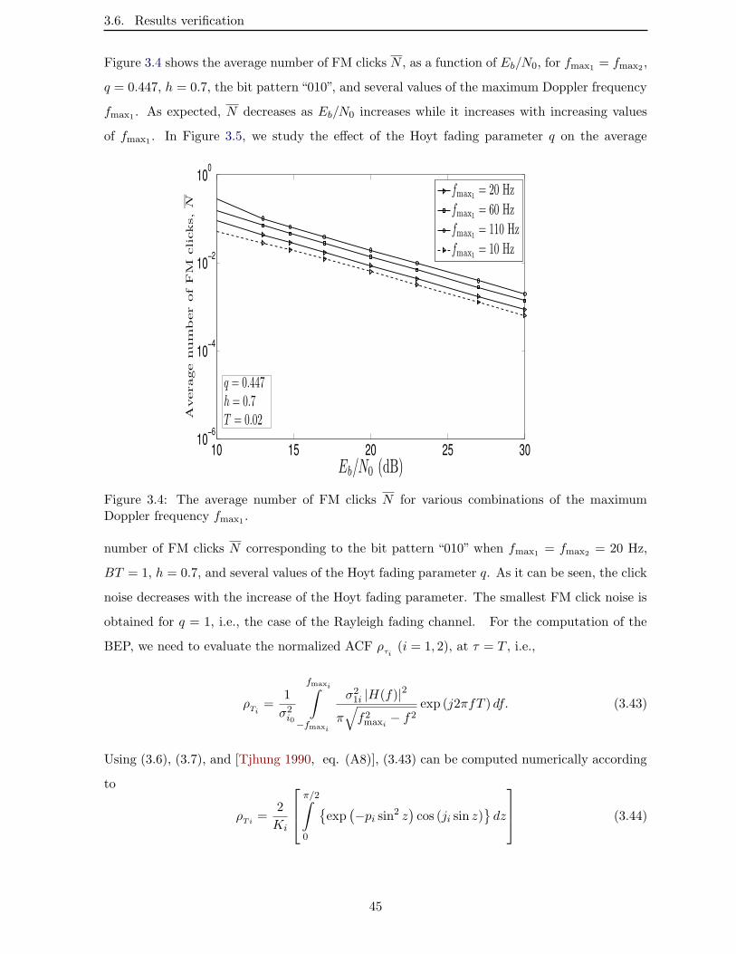
3.6. Results verification
Figure 3.4 shows the average number of FM clicks N , as a function of Eb/N0, for fmax1 = fmax2 ,
q = 0.447, h = 0.7, the bit pattern “010”, and several values of the maximum Doppler frequency
fmax1 . As expected, N decreases as Eb/N0 increases while it increases with increasing values
of fmax1 . In Figure 3.5, we study the effect of the Hoyt fading parameter q on the average
10 15 20 25 3010−6
10−4
10−2
100
Eb/N0 (dB)
Average
nu
mb
er
of
FM
cli
cks,N
fmax1 = 20 Hz
fmax1 = 60 Hz
fmax1= 110 Hz
fmax1 = 10 Hz
q = 0.447h = 0.7T = 0.02
Figure 3.4: The average number of FM clicks N for various combinations of the maximumDoppler frequency fmax1 .
number of FM clicks N corresponding to the bit pattern “010” when fmax1 = fmax2 = 20 Hz,
BT = 1, h = 0.7, and several values of the Hoyt fading parameter q. As it can be seen, the click
noise decreases with the increase of the Hoyt fading parameter. The smallest FM click noise is
obtained for q = 1, i.e., the case of the Rayleigh fading channel. For the computation of the
BEP, we need to evaluate the normalized ACF ρτi(i = 1, 2), at τ = T , i.e.,
ρTi=
1
σ2i0
fmaxi∫
−fmaxi
σ21i |H(f)|2
π√f2maxi − f2
exp (j2πfT ) df. (3.43)
Using (3.6), (3.7), and [Tjhung 1990, eq. (A8)], (3.43) can be computed numerically according
to
ρTi =2
Ki
π/2∫
0
exp
(−pi sin2 z
)cos (ji sin z)
dz
(3.44)
45
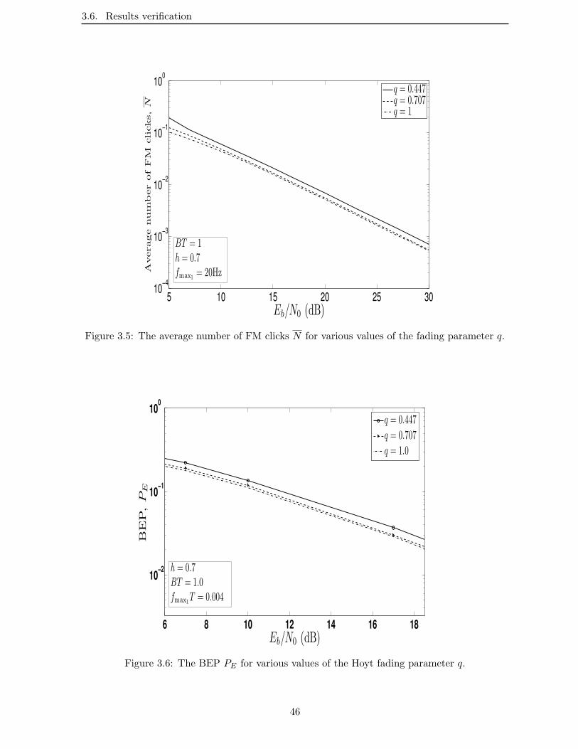
3.6. Results verification
5 10 15 20 25 3010−4
10−3
10−2
10−1
100
Eb/N0 (dB)
Average
nu
mb
er
of
FM
cli
cks,N
q = 0.447q = 0.707q = 1
BT = 1h = 0.7fmax1 = 20Hz
Figure 3.5: The average number of FM clicks N for various values of the fading parameter q.
6 8 10 12 14 16 18
10−2
10−1
100
Eb/N0 (dB)
BE
P,PE
q = 0.447
q = 0.707
q = 1.0
h = 0.7BT = 1.0fmax1T = 0.004
Figure 3.6: The BEP PE for various values of the Hoyt fading parameter q.
46

3.7. Conclusion
10 15 20 25 30 35 40 45 50 5510−5
10−4
10−3
10−2
10−1
100
Eb/N0 (dB)
BE
P,PE
BT = 1.0BT = 2.0BT = 3.0
q = 0.447h = 0.7fmax1T = 0.004
Figure 3.7: The BEP PE for various values of BT .
where pi = π (fmaxiT )2/(BT )
2, and ji = 2πfmaxiT . In Figure 3.6, the average BEP is plotted
versus Eb/N0 for h = 0.7, BT = 1, fmax1T = fmax2T = 0.004, and several values of the
fading parameter q. As can be seen, the error performance improves if q increases. The best
performance is obtained when q = 1, i.e., the case of the Rayleigh fading model. Figure 3.7
represents the average BEP PE , as a function of Eb/N0, for q = 0.447, h = 0.7, fmax1T =
fmax2T = 0.004, and BT = 1, 2, and 3. It can be noted from this figure that the performance
improves with decreasing the values of the product BT .
3.7 Conclusion
In this chapter, a performance analysis for narrowband FM systems with an LDI detection has
been considered, in the case of the Hoyt fading channels. The PDF of the phase difference
between two Hoyt vectors, and that induced by the additive noise, as well as the average
number of FM clicks have been first derived. Based on all these quantities, an expression for
the corresponding BEP performance has been deduced. Then, numerical results have been
given, and by which the effects of the fading severity as well as the system parameters on the
average number of FM clicks and the BEP performance have been examined. However, the
methodology employed here consists of the determination, separately, of the PDF of the phase
difference introduced by the receiver noise and that due to the Hoyt fading channel. Then,
47
3.7. Conclusion
the resultant phase PDF, needed for the evaluation of the BEP expression, is calculated by a
convolution operation, which demands tedious numerical integrations. In addition, the obtained
BEP results are valid only for small values of the SNR ratio and is restricted only for the Doppler
PSD of Jakes’ model.
To avoid the drawback of the method mentioned above, we will approach the problem of the
BEP performance of FSK modulation with the LDI detection over the Hoyt fading channels
from a different point of view. We will derive a closed-form expression for the PDF of the overall
phase difference of a modulated Hoyt faded signal corrupted by additive Gaussian noise. The
presentation of much more details on this new method will be the subject of the next chapter.
48

Chapter 4
PDF of the phase difference between
two Hoyt processes perturbed by
Gaussian noise
For various digital modulation schemes, especially the DPSK and FSK with LDI and differential
detection schemes, the decision variable needed for the demodulator is the differential phase,
over a symbol period, of the received faded signal perturbed by the Gaussian noise [Pawula 1981,
Xiong 2006]. For error rate calculations, an expression for the PDF of a such phase difference
is a vital information. Several previous works have considered the distribution of the phase
angle between two faded vectors perturbed by Gaussian noise. The earliest published work has
been presented in [Voelcker 1960], in which Voelcker derived the PDF of the phase difference
between two Rayleigh fading processes. This PDF has, then, been applied in the investigation
of the error rate performance of the PSK modulation over Rayleigh fading channels perturbed
by the Gaussian noise. Apart from the PDF distribution, the CDF of the corresponding phase
difference variable, can also be used in the calculation of the BEP performance of digital wireless
communications over fading channels. In this framework, an expression for the CDF of the phase
difference between two non-faded signals, each perturbed by the additive Gaussian noise has
been derived in [Pawula 1982]. This CDF has been widely used in the error rate analysis of
M -ary DPSK (MDPSK) modulation schemes, as it examplified in [Mason 1987]. Then, the
analysis on the CDF has been extended to the case of Rayleigh [Adachi 1992] and Nakagami
faded signals [Fedele 1995]. Recently, Chai [Chai 1999] derived new expressions for the CDF of
the phase difference between two signals perturbed by additive Gaussian noise, for mobile radio
communications characterized by the so-called Rice-lognormal channels, i.e., Rician fading and
lognormal shadowing, and Nakagami-lognormal channels, i.e., Nakagami fading and lognormal
shadowing. From the literature above, only the PDF and CDF of the phase difference between
two faded signals for the classical multipath fading models have been considered. To the best of
our knowledge, for the case of the Hoyt fading channels, there exist no results on the distribution
49
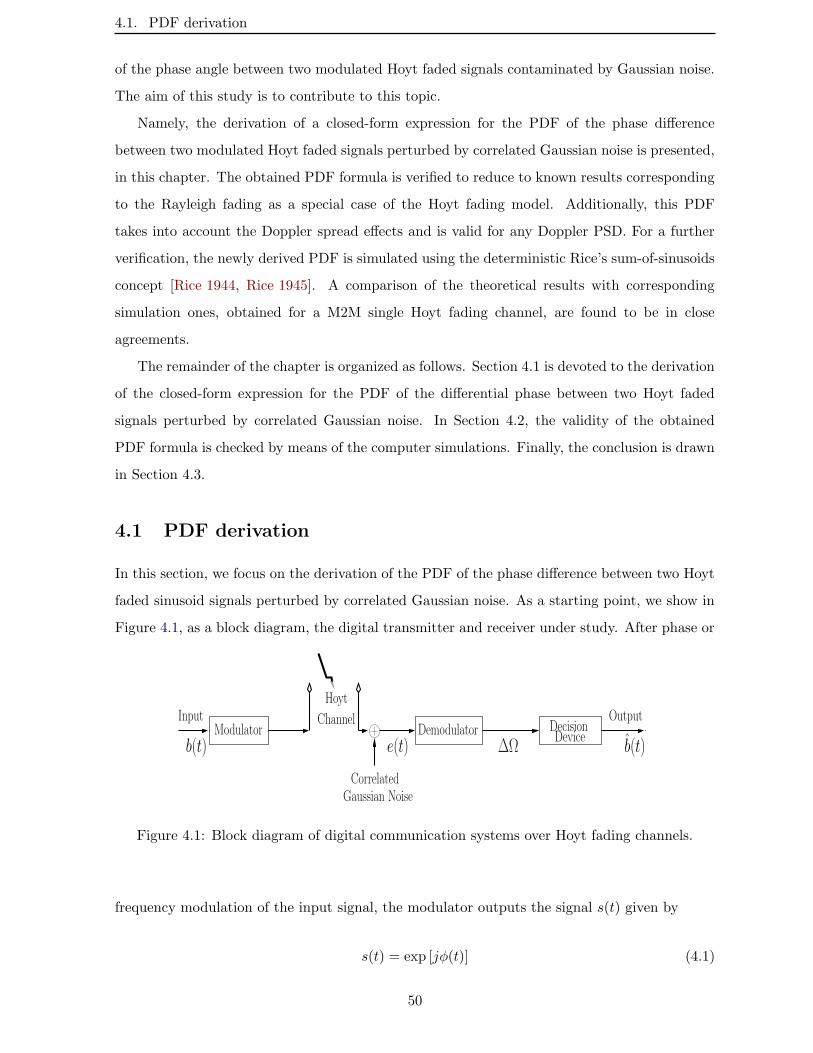
4.1. PDF derivation
of the phase angle between two modulated Hoyt faded signals contaminated by Gaussian noise.
The aim of this study is to contribute to this topic.
Namely, the derivation of a closed-form expression for the PDF of the phase difference
between two modulated Hoyt faded signals perturbed by correlated Gaussian noise is presented,
in this chapter. The obtained PDF formula is verified to reduce to known results corresponding
to the Rayleigh fading as a special case of the Hoyt fading model. Additionally, this PDF
takes into account the Doppler spread effects and is valid for any Doppler PSD. For a further
verification, the newly derived PDF is simulated using the deterministic Rice’s sum-of-sinusoids
concept [Rice 1944, Rice 1945]. A comparison of the theoretical results with corresponding
simulation ones, obtained for a M2M single Hoyt fading channel, are found to be in close
agreements.
The remainder of the chapter is organized as follows. Section 4.1 is devoted to the derivation
of the closed-form expression for the PDF of the differential phase between two Hoyt faded
signals perturbed by correlated Gaussian noise. In Section 4.2, the validity of the obtained
PDF formula is checked by means of the computer simulations. Finally, the conclusion is drawn
in Section 4.3.
4.1 PDF derivation
In this section, we focus on the derivation of the PDF of the phase difference between two Hoyt
faded sinusoid signals perturbed by correlated Gaussian noise. As a starting point, we show in
Figure 4.1, as a block diagram, the digital transmitter and receiver under study. After phase or
b(t)Modulator
InputDecisionDevice
Output
∆Ωe(t)
Hoyt
ChannelDemodulator
Gaussian NoiseCorrelated
b(t)
Figure 4.1: Block diagram of digital communication systems over Hoyt fading channels.
frequency modulation of the input signal, the modulator outputs the signal s(t) given by
s(t) = exp [jφ(t)] (4.1)
50
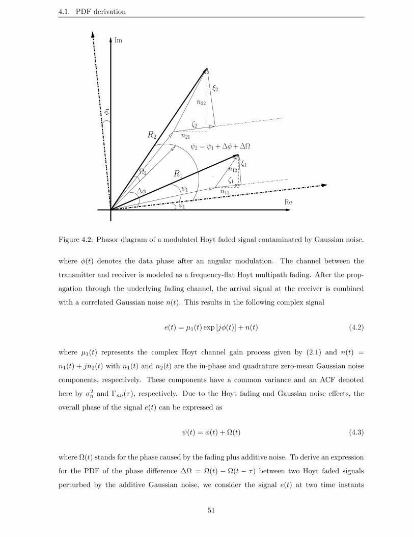
4.1. PDF derivation
φ1
R2
n11
n22
n21
n12Ω2
∆φ
φ1
ψ1
ξ1
ζ2
ξ2
ψ2 = ψ1 +∆φ +∆Ω
R1ζ1
Im
Re
Figure 4.2: Phasor diagram of a modulated Hoyt faded signal contaminated by Gaussian noise.
where φ(t) denotes the data phase after an angular modulation. The channel between the
transmitter and receiver is modeled as a frequency-flat Hoyt multipath fading. After the prop-
agation through the underlying fading channel, the arrival signal at the receiver is combined
with a correlated Gaussian noise n(t). This results in the following complex signal
e(t) = µ1(t) exp [jφ(t)] + n(t) (4.2)
where µ1(t) represents the complex Hoyt channel gain process given by (2.1) and n(t) =
n1(t) + jn2(t) with n1(t) and n2(t) are the in-phase and quadrature zero-mean Gaussian noise
components, respectively. These components have a common variance and an ACF denoted
here by σ2n and Γnn(τ), respectively. Due to the Hoyt fading and Gaussian noise effects, the
overall phase of the signal e(t) can be expressed as
ψ(t) = φ(t) + Ω(t) (4.3)
where Ω(t) stands for the phase caused by the fading plus additive noise. To derive an expression
for the PDF of the phase difference ∆Ω = Ω(t) − Ω(t − τ) between two Hoyt faded signals
perturbed by the additive Gaussian noise, we consider the signal e(t) at two time instants
51

4.1. PDF derivation
t1 = t− τ and t2 = t, i.e., e(t1) and e(t2). By assuming a coordinate system that rotates with
a phase angle φ1 = φ(t1) as shown in Figure 4.2, we may write for the processes e(t1) and e(t2)
the following quantities given by
z1 = (µ11 + ζ1) + j (µ12 + ξ1)
= x1 + jy1
= R1 exp [jψ1] (4.4)
and
z2 = (µ21 cos(∆φ)− µ22 sin(∆φ) + ζ2) + j (µ21 sin(∆φ) + µ22 cos(∆φ) + ξ2)
= x2 + jy2
= R2 exp [jψ2] (4.5)
respectively. In the above expressions, ∆φ = φ(t) − φ(t − τ) is the data phase difference,
µ1i = µ1i(t1) and µ2i = µ1i(t2) (i = 1, 2). Also in (4.4) and (4.5), the processes ζi and ξi
(i = 1, 2) denote the noise components defined relatively to the coordinate system that rotates
with φ1, and are, respectively, related to the noise components n1i = ni(t1), and n2i = ni(t2)
(i = 1, 2) according to
ζi =ni1 cos(φ1) + ni2 sin(φ1) (4.6)
and
ξi =ni2 cos(φ1)− ni1 sin(φ1). (4.7)
It can easily be shown that these components are zero-mean independent Gaussian random
variables having the same variance σ2n and the ACF Γnn(τ) corresponding to that of the noise
nij (i, j = 1, 2). Thus, it may be concluded that, in this new coordinate system, the statistical
properties of the resulting noise components ξi and ζi remain unchanged with respect to those
of nij (i, j = 1, 2). For the sake of convenience, we denote the quantities µ11 + ζ1 and µ12 + ξ1,
respectively, by x1 and y1, for the quadrature components of the signal z1. Similarly, for z2,
we denote the quantities µ21 cos(∆φ)− µ22 sin(∆φ) + ζ2 and µ21 sin(∆φ) + µ22 cos(∆φ) + ξ2 by
x2 and y2, respectively. From expressions (4.4) and (4.5), we can note that xi and yi (i = 1, 2)
are combinations of Gaussian processes. Hence, for a given information symbol ∆φ, they are
52
4.1. PDF derivation
Gaussian distributed as well. Since we assume a symmetrical Doppler PSD for the Hoyt fading
and uncorrelated additive noise, we have
E µ11µ12 = E µ21µ22 = E ζ1ξ1 = E ζ2ξ2 = 0. (4.8)
Furthermore, assuming that the signal component is independent of the noise component allows
us to obtain the following expressions for the cross-correlation quantities of the variables x1, y1,
x2, and y2
a12 = E x1y1 = 0
a14 = E x1y2 = Γµ11µ11(τ) sin(∆φ)
a32 = E x2y1 = −Γµ12µ12(τ) sin(∆φ)
a34 = E x2y2 = σ211(1− q2
)cos(∆φ) sin(∆φ)
a13 = E x1x2 = Γµ11µ11(τ) cos(∆φ) + Γnn(τ)
a24 = E y1y2 = Γµ12µ12(τ) cos(∆φ) + Γnn(τ) (4.9)
where Γµ1iµ1i(τ) (i = 1, 2) represents the ACF of the process µ1i(t) (i = 1, 2). Concerning the
mean power of the underlying Gaussian processes, it is found to be given by
σ2x1 =Ex21= σ2n (Λ + 1)
σ2y1 =Ey21= σ2n
(q2Λ + 1
)
σ2x2 =Ex22= σ2n
(Λcos2(∆φ) + q2 sin2(∆φ)
+ 1)
σ2y2 =Ey22= σ2n
(Λsin2(∆φ) + q2 cos2(∆φ)
+ 1)
(4.10)
where the parameter Λ = σ211/σ
2n. Finally, in addition to the quadrature signal based description
presented above, we introduce the quantities Ri =√x2i + y2i and ψi = tan−1(yi/xi)(i = 1, 2),
to denote, respectively, the overall envelope and phase of the modulated Hoyt faded signal con-
taminated by correlated Gaussian noise. As it has previously been mentioned, we are concerned
mostly with the derivation of the PDF p∆Ω(ϕ) of the phase difference ∆Ω due to the Hoyt fad-
ing plus an additive noise. A starting point for the derivation of this PDF is the determination
of the joint PDF px1y1x2y2(ν1, ν2, ν3, ν4) of the Gaussian random variables x1, y1, x2, and y2.
Based on the multivariate Gaussian distribution, the joint PDF px1y1x2y2(ν1, ν2, ν3, ν4) can be
53
4.1. PDF derivation
written as
px1y1x2y2(ν1, ν2, ν3, ν4) =1
(2π)2√detΣ
exp[(ν1, ν2, ν3, ν4)
H Σ−1 (ν1, ν2, ν3, ν4)]
(4.11)
where Σ represents the covariance matrix of the vector process (x1, y1, x2, y2)H and in which H
stands for the transpose operator. Also, in (4.11) Σ−1 is the inverse matrix of the covariance
matrix Σ and detΣ denotes the determinant of Σ. Using (4.9) and (4.10), the covariance matrix
Σ can be expressed as
Σ =
σ2x1 0 a13 a14
0 σ2y1 a23 a24
a13 a23 σ2x2 a34
a14 a24 a34 σ2y2
. (4.12)
After some algebraic manipulations, the determinant of this matrix, i.e., detΣ, is found to be
given by
detΣ = σ2x1σ2y1σ
2x2σ
2y2 ·K (4.13)
where the quantity K is expressed as a function of the correlation quantities of the variables
x1, y1, x2, and y2 and is shown in the Appendix B. Then, a calculation of the inverse matrix of
Σ gives
Σ−1 =1
detΣ
χ11 −χ12 χ13 −χ14
−χ12 χ22 −χ23 χ24
χ13 −χ23 χ33 −χ34
−χ14 χ13 −χ34 χ44
(4.14)
where the parameters χij (i; j = 1, . . . , 4) are listed in the Appendix B. Therefore, substitut-
ing (4.13) and (4.14) in (4.11) and doing some algebraic manipulations yields the following
expression for the joint PDF px1y1x2y2(ν1, ν2, ν3, ν4) of the variables x1, y1, x2, and y2
px1y1x2y2(ν1, ν2, ν3, ν4) =B1 exp[−B2
[(χ11ν
21 + χ22ν
22 + 2χ12ν1ν2
)
+(χ33ν
23 + χ44ν
24 + 2χ34ν3ν4
)
− 2 (ν1 χ13ν3 + χ14ν4 +ν2 χ23ν3 + χ24ν4)]] (4.15)
54
4.1. PDF derivation
where the quantities B1 and B2 are given by
B1 =1
4π2σx1σy1σx2σy2K1/2
, B2 =1
2K. (4.16)
Now, the transformation of the Cartesian coordinates (x, y), to polar coordinates (R,ψ), results
in the following expression for the joint PDF pR1R2ψ1ψ2(z1, z2, ϕ1, ϕ2) of the random variables
R1, R2, ψ1, and ψ2, according to
pR1R2ψ1ψ2(z1, z2, ϕ1, ϕ2) =B1z1z2 exp
[−B2
[(χ11 cos
2 ϕ1 + χ22 sin2 ϕ1 +2χ12 cosϕ1 sinϕ1) z
21
+(χ33 cos
2 ϕ2 + χ44 sin2 ϕ2 +2χ34 cosϕ2 sinϕ2) z
22 − 2 (cosϕ1
× χ13 cosϕ2 + χ14 sinϕ2+ sinϕ1 χ23 cosϕ2 + χ24 sinϕ2) z1z2]] .(4.17)
Then, the joint PDF pψ1ψ2(ϕ1, ϕ2) of the random phases ψ1 and ψ2 can be obtained by solving
the integrals over the joint PDF pR1R2ψ1ψ2(R1, R2, ϕ1, ϕ2) as follows
pψ1ψ2(ϕ1, ϕ2) =
∞∫
0
∞∫
0
pR1R2ψ1ψ2(z1, z2, ϕ1, ϕ2)dz1dz2. (4.18)
The double integral involved in (4.18) can be solved by making use of the multiple integrals evalu-
ation approach, which has previously been described in Section 3.2 of chapter 3. The application
of this approach yields the following closed-form expression for the joint PDF pψ1ψ2(ϕ1, ϕ2) of
the phases ψ1 and ψ2
pψ1ψ2(ϕ1, ϕ2) =
B1
4B22
1(E1F1 −D2
1
) ×(1 +
D1(E1F1 −D2
1
)1/2
×[π
2+ tan−1
(D1(
E1F1 −D21
)1/2
)])(4.19)
where the quantities D1, E1, and F1 are given by
D1 =cosϕ1 χ13 cosϕ2 + χ14 sinϕ2+ sinϕ1 χ23 cosϕ2 + χ24 sinϕ2
E1 =χ11 cos2 ϕ1 + χ22 sin
2 ϕ1 + 2χ12 cosϕ1 sinϕ1
F1 =χ33 cos2 ψ2 + χ44 sin
2 ψ2 + 2χ34 cosϕ2 sinϕ2. (4.20)
It can be verified that, for q = 1 and ∆φ = 0, i.e., the case corresponding to the transmission
of an unmodulated over the Rayleigh fading channels, by using the help of [Gradshteyn 1994,
55
4.2. Simulation and results verification
eq.1.624 (2)] and doing algebraic manipulations, (4.19) simplifies to
pψ1ψ2(ϕ1, ϕ2) =
1− ρ2µ11+n
4π2(1− (ρµ11+n cos (ϕ2 − ϕ1))
2)
1 + ρµ11+n cos (ϕ2 − ϕ1)√
1− (ρµ11+n cos (ϕ2 − ϕ1))2
×(π2+ sin−1 (ρµ11+n cos (ϕ2 − ϕ1))
)](4.21)
where the quantity ρµ11+n represents the normalized ACF of the process (µ11(t) +n1(t)) and is
given by
ρµ11+n =
(Γµ11µ11(τ) + Γnn(τ)
σ211+ σ2n
). (4.22)
It should be noted that the simplified joint PDF is in agreement with the already known result
[Bramley 1951, eq. (33)]. To the best of our knowledge, (4.19) is new and it constitutes
the basis for the determination of the PDF p∆Ω(ϕ). In fact, using (4.19) and noting that
ψ2 − ψ1 = ∆φ +∆Ω, allows us to obtain the desired PDF p∆Ω(ϕ) of the phase difference ∆Ω
according to
p∆Ω(ϕ) =
π∫
−π
pψ1ψ2(ϕ1, ϕ1 +∆φ+ ϕ)dϕ1. (4.23)
Unfortunately, the finite range integration involved in (4.23) is difficult to handle, and it can
be evaluated only by using numerical techniques. For the special case given by q = 1, i.e., the
Rayleigh channel case, the underlying integral is easily solved and it is found that (4.23) is in
agreement with the result [Adachi 1992, eq.(4)]. Furthermore, for q = 1 and ∆φ = 0, (4.23)
simplifies to
p∆Ω(ϕ) =1− ρ2µ11+n
2π(1− (ρµ11+n cos (ϕ))
2)
1 + ρµ11+n cos (ϕ)√
1− (ρµ11+n cos (ϕ))2
(π2+ sin−1 (ρµ11+n cos (ϕ))
)]
(4.24)
which corresponds perfectly to [Bramley 1951, eq. (34)].
4.2 Simulation and results verification
In this section, we check the validity of the derived PDF p∆Ω(ϕ) based on the computer sim-
ulation results obtained for the case of a M2M single Hoyt fading channel. For this channel
type, as it has previously been reviewed in chapter 2, the ACF Γµ1iµ1i(τ) of the process µ1i(t)
56
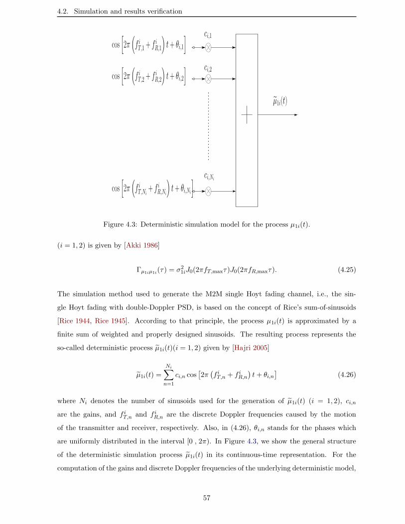
4.2. Simulation and results verification
ci,2
µ1i(t)
ci,Ni
cos[2π(f iT,Ni
+ f iR,Ni
)t + θi,Ni
]
cos[2π(f iT,2 + f iR,2
)t + θi,2
]
cos[2π(f iT,1 + f iR,1
)t + θi,1
] ci,1
Figure 4.3: Deterministic simulation model for the process µ1i(t).
(i = 1, 2) is given by [Akki 1986]
Γµ1iµ1i(τ) = σ21iJ0(2πfT,maxτ)J0(2πfR,maxτ). (4.25)
The simulation method used to generate the M2M single Hoyt fading channel, i.e., the sin-
gle Hoyt fading with double-Doppler PSD, is based on the concept of Rice’s sum-of-sinusoids
[Rice 1944, Rice 1945]. According to that principle, the process µ1i(t) is approximated by a
finite sum of weighted and properly designed sinusoids. The resulting process represents the
so-called deterministic process µ1i(t)(i = 1, 2) given by [Hajri 2005]
µ1i(t) =
Ni∑
n=1
ci,n cos[2π(f iT,n + f iR,n
)t+ θi,n
](4.26)
where Ni denotes the number of sinusoids used for the generation of µ1i(t) (i = 1, 2), ci,n
are the gains, and f iT,n and f iR,n are the discrete Doppler frequencies caused by the motion
of the transmitter and receiver, respectively. Also, in (4.26), θi,n stands for the phases which
are uniformly distributed in the interval [0 , 2π). In Figure 4.3, we show the general structure
of the deterministic simulation process µ1i(t) in its continuous-time representation. For the
computation of the gains and discrete Doppler frequencies of the underlying deterministic model,
57
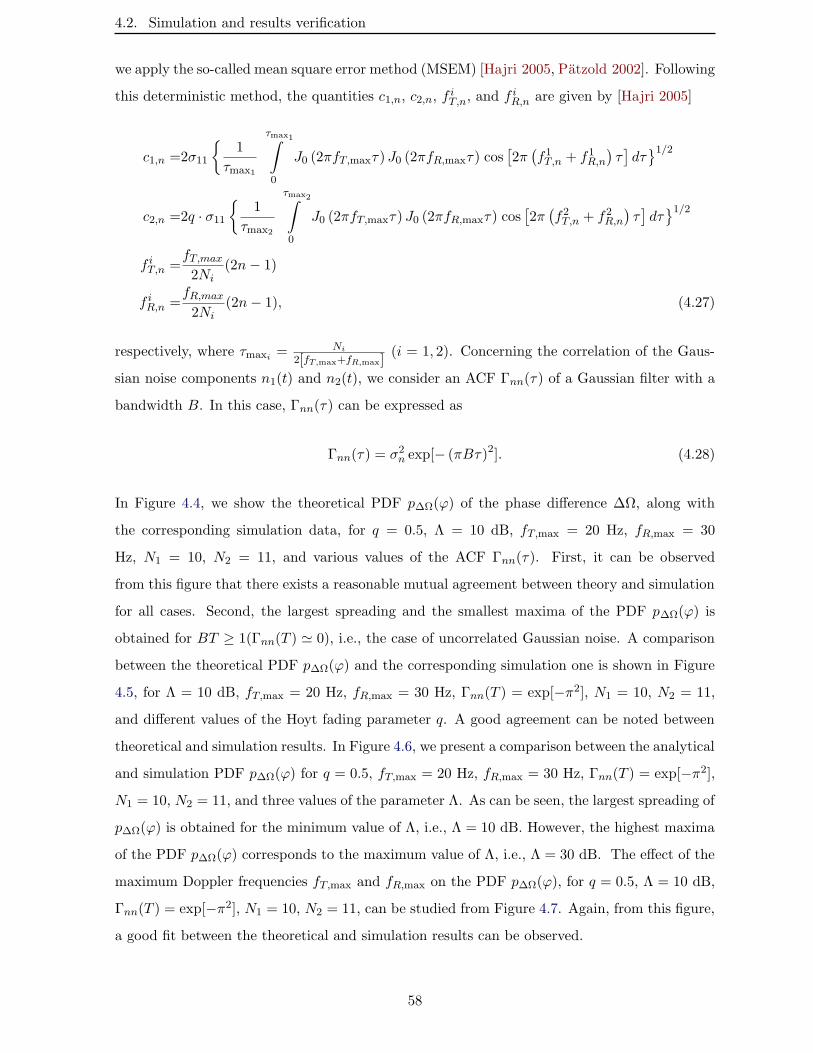
4.2. Simulation and results verification
we apply the so-called mean square error method (MSEM) [Hajri 2005, Patzold 2002]. Following
this deterministic method, the quantities c1,n, c2,n, fiT,n, and f
iR,n are given by [Hajri 2005]
c1,n =2σ11
1
τmax1
τmax1∫
0
J0 (2πfT,maxτ) J0 (2πfR,maxτ) cos[2π(f1T,n + f1R,n
)τ]dτ1/2
c2,n =2q · σ11
1
τmax2
τmax2∫
0
J0 (2πfT,maxτ) J0 (2πfR,maxτ) cos[2π(f2T,n + f2R,n
)τ]dτ1/2
f iT,n =fT,max2Ni
(2n− 1)
f iR,n =fR,max2Ni
(2n− 1), (4.27)
respectively, where τmaxi =Ni
2[fT,max+fR,max](i = 1, 2). Concerning the correlation of the Gaus-
sian noise components n1(t) and n2(t), we consider an ACF Γnn(τ) of a Gaussian filter with a
bandwidth B. In this case, Γnn(τ) can be expressed as
Γnn(τ) = σ2n exp[− (πBτ)2]. (4.28)
In Figure 4.4, we show the theoretical PDF p∆Ω(ϕ) of the phase difference ∆Ω, along with
the corresponding simulation data, for q = 0.5, Λ = 10 dB, fT,max = 20 Hz, fR,max = 30
Hz, N1 = 10, N2 = 11, and various values of the ACF Γnn(τ). First, it can be observed
from this figure that there exists a reasonable mutual agreement between theory and simulation
for all cases. Second, the largest spreading and the smallest maxima of the PDF p∆Ω(ϕ) is
obtained for BT ≥ 1(Γnn(T ) ' 0), i.e., the case of uncorrelated Gaussian noise. A comparison
between the theoretical PDF p∆Ω(ϕ) and the corresponding simulation one is shown in Figure
4.5, for Λ = 10 dB, fT,max = 20 Hz, fR,max = 30 Hz, Γnn(T ) = exp[−π2], N1 = 10, N2 = 11,
and different values of the Hoyt fading parameter q. A good agreement can be noted between
theoretical and simulation results. In Figure 4.6, we present a comparison between the analytical
and simulation PDF p∆Ω(ϕ) for q = 0.5, fT,max = 20 Hz, fR,max = 30 Hz, Γnn(T ) = exp[−π2],N1 = 10, N2 = 11, and three values of the parameter Λ. As can be seen, the largest spreading of
p∆Ω(ϕ) is obtained for the minimum value of Λ, i.e., Λ = 10 dB. However, the highest maxima
of the PDF p∆Ω(ϕ) corresponds to the maximum value of Λ, i.e., Λ = 30 dB. The effect of the
maximum Doppler frequencies fT,max and fR,max on the PDF p∆Ω(ϕ), for q = 0.5, Λ = 10 dB,
Γnn(T ) = exp[−π2], N1 = 10, N2 = 11, can be studied from Figure 4.7. Again, from this figure,
a good fit between the theoretical and simulation results can be observed.
58
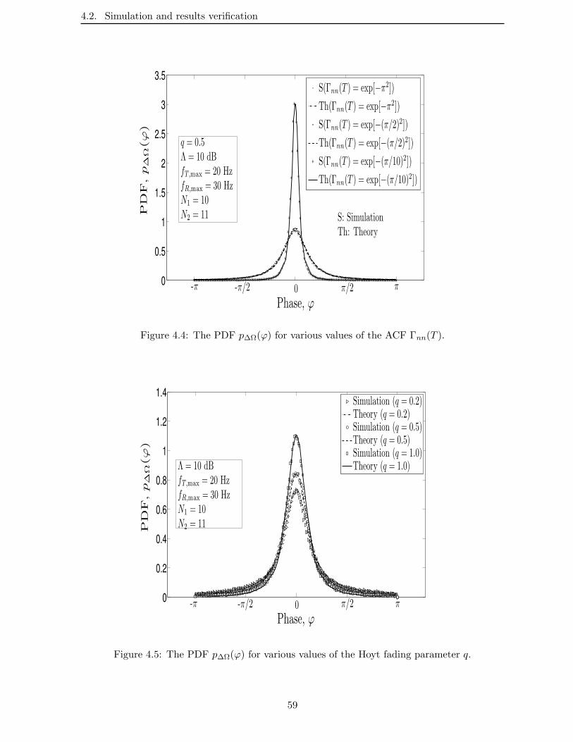
4.2. Simulation and results verification
0
0.5
1
1.5
2
2.5
3
3.5
Phase, ϕ
PD
F,p
∆Ω
(ϕ
)
S(Γnn(T ) = exp[−π2])
Th(Γnn(T ) = exp[−π2])
S(Γnn(T ) = exp[−(π/2)2])
Th(Γnn(T ) = exp[−(π/2)2])
S(Γnn(T ) = exp[−(π/10)2])
Th(Γnn(T ) = exp[−(π/10)2])
q = 0.5Λ = 10 dBfT,max = 20 HzfR,max = 30 HzN1 = 10N2 = 11 S: Simulation
Th: Theory
-π -π/2 ππ/20
Figure 4.4: The PDF p∆Ω(ϕ) for various values of the ACF Γnn(T ).
0
0.2
0.4
0.6
0.8
1
1.2
1.4
Phase, ϕ
PD
F,p
∆Ω
(ϕ
)
Simulation (q = 0.2)Theory (q = 0.2)Simulation (q = 0.5)Theory (q = 0.5)Simulation (q = 1.0)Theory (q = 1.0)Λ = 10 dB
fT,max = 20 HzfR,max = 30 HzN1 = 10N2 = 11
-π -π/2 ππ/20
Figure 4.5: The PDF p∆Ω(ϕ) for various values of the Hoyt fading parameter q.
59
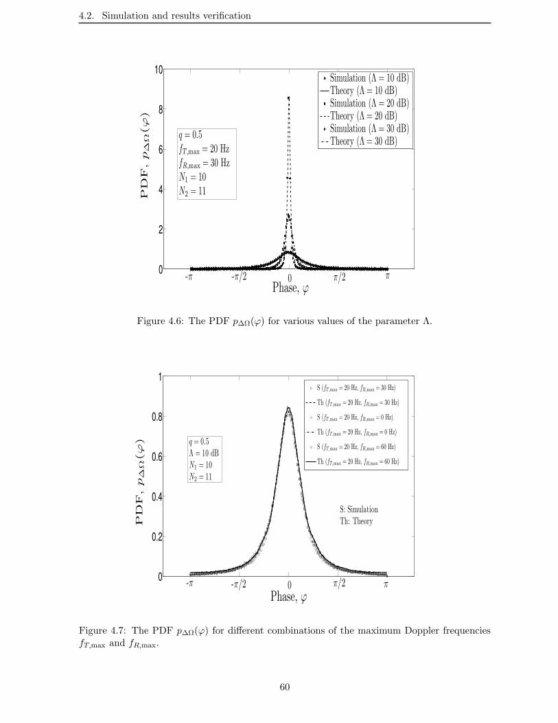
4.2. Simulation and results verification
0
2
4
6
8
10
Phase, ϕ
PD
F,p
∆Ω
(ϕ
)
Simulation (Λ = 10 dB)Theory (Λ = 10 dB)Simulation (Λ = 20 dB)Theory (Λ = 20 dB)Simulation (Λ = 30 dB)Theory (Λ = 30 dB)
q = 0.5fT,max = 20 HzfR,max = 30 HzN1 = 10N2 = 11
-π -π/2 π/2 π0
Figure 4.6: The PDF p∆Ω(ϕ) for various values of the parameter Λ.
0
0.2
0.4
0.6
0.8
1
Phase, ϕ
PD
F,p
∆Ω
(ϕ
)
S (fT,max = 20 Hz, fR,max = 30 Hz)
Th (fT,max = 20 Hz, fR,max = 30 Hz)
S (fT,max = 20 Hz, fR,max = 0 Hz)
Th (fT,max = 20 Hz, fR,max = 0 Hz)
S (fT,max = 20 Hz, fR,max = 60 Hz)
Th (fT,max = 20 Hz, fR,max = 60 Hz)
S: SimulationTh: Theory
q = 0.5Λ = 10 dBN1 = 10N2 = 11
-π -π/2 π/2 π0
Figure 4.7: The PDF p∆Ω(ϕ) for different combinations of the maximum Doppler frequenciesfT,max and fR,max.
60
4.3. Conclusion
4.3 Conclusion
In this chapter, a closed-form expression for the PDF of the phase difference between two Hoyt
faded signals perturbed by the correlated Gaussian noise has been derived. The obtained PDF
expression is verified to reduce to known results corresponding to the Rayleigh fading as a
special case of the Hoyt fading model. Furthermore, the validity of the presented results has
been checked by computer simulations, obtained for a M2M single Hoyt fading channel. The
newly derived PDF formula can then be applied in the evaluation of the error rate performance
of wireless M2M communications over the single Hoyt multipath fading channels with a double-
Doppler PSD.
Specifically, based on this PDF expression and drawing upon the theory on the BEP, the error
rate performance of the DPSK modulation schemes and FSK with the LDI and differential
detections are investigated. Much more details on the derivation of analytical expressions for
the BEP performance of the DPSK and FSK modulation schemes over the single Hoyt fading
channels with a double-Doppler PSD, i.e., the so-called M2M single Hoyt fading channels, will
be presented in the next chapter.
61
Chapter 5
BEP Performance of DPSK and
FSK modulation schemes over M2M
single Hoyt fading channels
Based upon the newly derived PDF formula for the phase difference between two Hoyt vectors
contaminated by AWGN, which has been presented in the previous chapter, and the theory of
digital modulations together with that of the error rate performance, the BEP performance of
the DPSKmodulation schemes and FSK with the LDI and differential detections are investigated
and analyzed. Namely, analytical expressions for the BEP performance of all these modulation
schemes over the Hoyt multipath fading channels, taking into account the Doppler spread effects
caused by the motion of the mobile transmitter and receiver, are derived.
The objective of this chapter is to present all details on the derivation of these analytical BEP
expressions, considering the case of M2M single Hoyt fading channels, i.e., the case of Hoyt
multipath fading channels with a double-Doppler PSD.
The remainder of the chapter is organized as follows. In Section 5.1, a study on the BEP
performance of the DPSK modulation schemes over frequency-flat M2M single Hoyt fading
channels is presented. The performance analysis of the FSK modulation with an LDI detection
over the same M2M channels is studied, in Section 5.2. The BEP of the one-bit delay differential
detection of narrowband FSK signals transmitted over M2M single Hoyt fading channels is
provided, in Section 5.3. Finally, Section 5.4 concludes the chapter.
5.1 Performance analysis of DPSK modulation schemes
The objective of this section is to provide an analysis on the BEP performance of the DPSK
modulation over the so-called M2M single Hoyt fading channels. The derivation of an analytical
expression for the corresponding BEP is carried out by applying the theory of the DPSK mod-
ulation [Voelcker 1960, Miyagaki 1979], and using the recently derived PDF formula in chapter
62
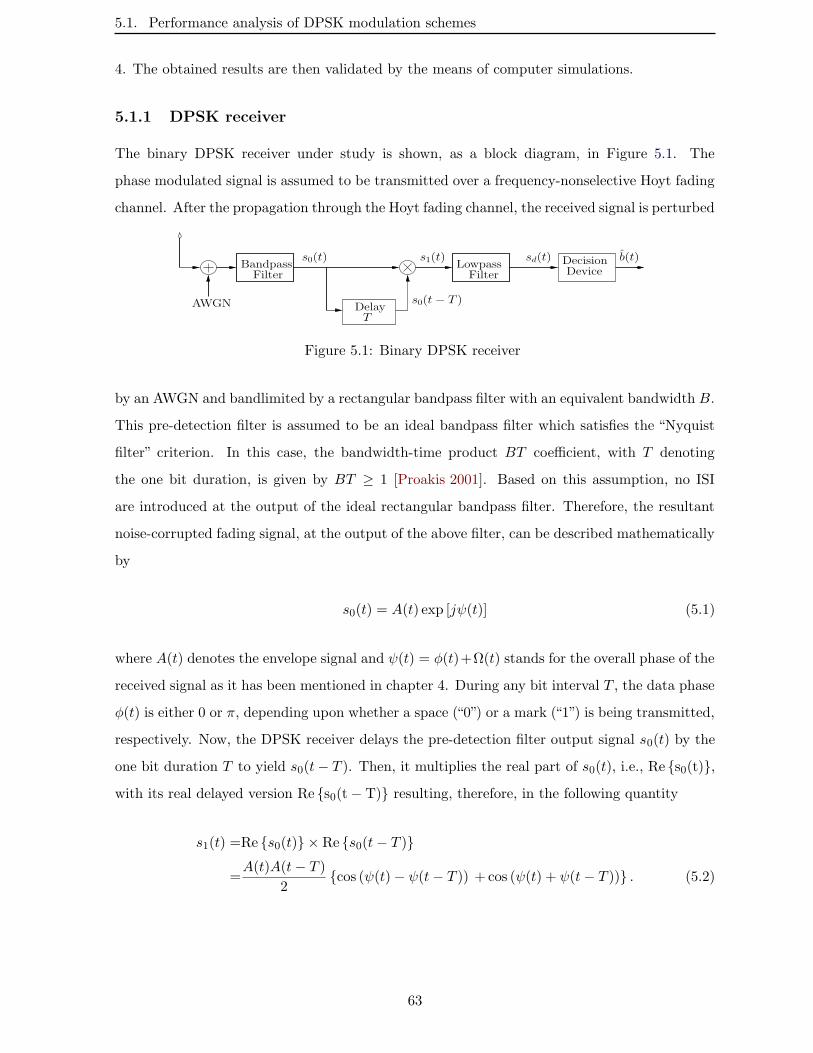
5.1. Performance analysis of DPSK modulation schemes
4. The obtained results are then validated by the means of computer simulations.
5.1.1 DPSK receiver
The binary DPSK receiver under study is shown, as a block diagram, in Figure 5.1. The
phase modulated signal is assumed to be transmitted over a frequency-nonselective Hoyt fading
channel. After the propagation through the Hoyt fading channel, the received signal is perturbed
Device
b(t)
Filter
AWGN
Filter
s0(t)
DelayT
s0(t− T )
s1(t) sd(t)Bandpass Lowpass Decision
Figure 5.1: Binary DPSK receiver
by an AWGN and bandlimited by a rectangular bandpass filter with an equivalent bandwidth B.
This pre-detection filter is assumed to be an ideal bandpass filter which satisfies the “Nyquist
filter” criterion. In this case, the bandwidth-time product BT coefficient, with T denoting
the one bit duration, is given by BT ≥ 1 [Proakis 2001]. Based on this assumption, no ISI
are introduced at the output of the ideal rectangular bandpass filter. Therefore, the resultant
noise-corrupted fading signal, at the output of the above filter, can be described mathematically
by
s0(t) = A(t) exp [jψ(t)] (5.1)
where A(t) denotes the envelope signal and ψ(t) = φ(t)+Ω(t) stands for the overall phase of the
received signal as it has been mentioned in chapter 4. During any bit interval T , the data phase
φ(t) is either 0 or π, depending upon whether a space (“0”) or a mark (“1”) is being transmitted,
respectively. Now, the DPSK receiver delays the pre-detection filter output signal s0(t) by the
one bit duration T to yield s0(t− T ). Then, it multiplies the real part of s0(t), i.e., Re s0(t),with its real delayed version Re s0(t− T) resulting, therefore, in the following quantity
s1(t) =Re s0(t) × Re s0(t− T )
=A(t)A(t− T )
2cos (ψ(t)− ψ(t− T )) + cos (ψ(t) + ψ(t− T )) . (5.2)
63
5.1. Performance analysis of DPSK modulation schemes
Thereafter, the obtained signal in (5.2) is fed into a lowpass filter. After filtering the high
frequency terms, the post-detection filter outputs the signal given by
sd(t) =A(t)A(t− T )
2cos (∆ψ) (5.3)
where ∆ψ = ψ(t)− ψ(t− T ) stands for the overall phase difference and can be expressed as
∆ψ =φ(t)− φ(t− T ) + Ω(t)− Ω(t− T )
=∆φ+∆Ω. (5.4)
Finally, the filtered output signal sd(t) is sampled and fed into a decision device. Since the
envelope A(t) is always positive, the decision on whether a mark or a space is sent is essentially
based on the polarity of the quantity cos (∆ψ). Therefore, in order to analyze the error rate
performance of the binary DPSK modulation scheme, it is necessary to determine the PDF
p∆ψ(ϕ) of the phase difference ∆ψ. An expression for this PDF is given by
p∆ψ(ϕ) =
π∫
−π
pψ1ψ2(ϕ1, ϕ1 + ϕ)dϕ1 (5.5)
where pψ1ψ2(·, ·) is the joint PDF of the random phases ψ1 = φ(t − T ) + Ω(t − T ) and ψ2 =
φ(t) + Ω(t). An expression for this joint PDF has been derived in chapter 4, and is given by
(4.19). The PDF p∆ψ(ϕ) of the phase difference ∆ψ, is valid for any Doppler PSD, especially
for the Doppler PSD of the M2M Hoyt fading channels. In Figure 5.2, we show the PDF p∆ψ(ϕ)
of the phase difference ∆ψ, for BT = 1.0, ∆φ = π/3, Λ = 10 dB, fT,max ·T = fR,max ·T = 0.004,
and various values of the Hoyt fading parameter q. As it can be seen, the PDF is symmetrical
about ∆φ = π/3. In addition, the largest spreading of the PDF p∆ψ(ϕ) is obtained for q = 0,
i.e., the case of the one-sided Gaussian channel. However, the smallest one corresponds to the
Rayleigh fading channel, i.e., the case when q = 1.
5.1.2 Bit error probability
The average BEP performance of the DPSK modulation with a noncoherent detection can be
obtained according to [Lee 1975, Pawula 1984]
PE = pmPE (M) + (1− pm)PE (S) (5.6)
64
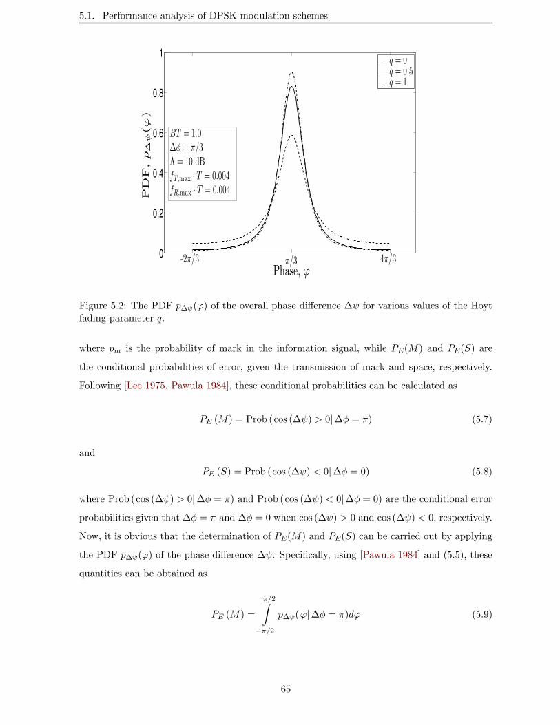
5.1. Performance analysis of DPSK modulation schemes
0
0.2
0.4
0.6
0.8
1
Phase, ϕ
PD
F,p
∆ψ
(ϕ
)
q = 0q = 0.5q = 1
-2π/3 π/3 4π/3
BT = 1.0∆φ = π/3Λ = 10 dBfT,max · T = 0.004fR,max · T = 0.004
Figure 5.2: The PDF p∆ψ(ϕ) of the overall phase difference ∆ψ for various values of the Hoytfading parameter q.
where pm is the probability of mark in the information signal, while PE(M) and PE(S) are
the conditional probabilities of error, given the transmission of mark and space, respectively.
Following [Lee 1975, Pawula 1984], these conditional probabilities can be calculated as
PE (M) = Prob (cos (∆ψ) > 0|∆φ = π) (5.7)
and
PE (S) = Prob (cos (∆ψ) < 0|∆φ = 0) (5.8)
where Prob (cos (∆ψ) > 0|∆φ = π) and Prob (cos (∆ψ) < 0|∆φ = 0) are the conditional error
probabilities given that ∆φ = π and ∆φ = 0 when cos (∆ψ) > 0 and cos (∆ψ) < 0, respectively.
Now, it is obvious that the determination of PE(M) and PE(S) can be carried out by applying
the PDF p∆ψ(ϕ) of the phase difference ∆ψ. Specifically, using [Pawula 1984] and (5.5), these
quantities can be obtained as
PE (M) =
π/2∫
−π/2
p∆ψ(ϕ|∆φ = π)dϕ (5.9)
65

5.1. Performance analysis of DPSK modulation schemes
and
PE (S) =
3π/2∫
π/2
p∆ψ(ϕ|∆φ = 0)dϕ. (5.10)
Unfortunately, the finite range integrations in (5.9) and (5.10) can be evaluated only by numer-
ical techniques. Finally, the desired BEP performance of the DPSK detection over the Hoyt
fading channels can be obtained by substituting (5.9) and (5.10) in (5.6). It should be noted
that for the special case when q = 1, i.e., the case of Rayleigh fading channels, the evaluation
of (5.6) using (5.9) and (5.10) leads to
PE =1
2
(1− Γµ11µ11(T ) + Γnn(T )
σ211 + σ2n+ 2pm
Γnn(T )
σ211 + σ2n
)(5.11)
which corresponds to the result reported in [Jakes 1993, Voelcker 1960].
5.1.3 Results verification
5.1.3.1 Simulation model
According to (2.1), the Hoyt channel gain can be simulated by the generation of two Gaus-
sian random processes. The simulation method used here to generate the process (2.1) is
based on the concept of Rice’s sum-of-sinusoids [Rice 1944, Rice 1945]. Following this con-
cept, the Gaussian process µ1i(t) (i = 1, 2) describing the Hoyt channel gain process µ1(t)
can be basically approximated using the deterministic process µ1i(t) as expressed in (4.26).
Again, for the computation of the parameters of the simulation model (4.26), i.e., the gains ci,n,
the discrete frequencies f iT,n and f iR,n, as well as the discrete phases θi,n, we use the MSEM
method [Hajri 2005, Patzold 2002]. These parameters have to be determined such that the ACF
Γµ1iµ1i(τ) of the reference M2M single Hoyt fading channel, which is described by (4.25), is well
approximated by that of the deterministic simulation model Γµ1iµ1i(τ) given by [Hajri 2005]
Γµ1iµ1i(τ) =
Ni∑
n=1
c2i,n2
cos[2π(f iT,n + f iR,n
)τ]. (5.12)
According to this deterministic method, the gains ci,n and the discrete frequencies f iT,n and f iR,n
(i = 1, 2) are given by (4.27). In Figure 5.3, we show a comparison between the ACF Γµ12µ12(τ)
of the reference model µ12(t) and that of the corresponding simulation model Γµ12µ12(τ), for
q = 0.5, N2 = 7, fT,max = 80 Hz, and fR,max = 20 Hz. As it can be seen, the theoretical results
are well supported by the corresponding simulation ones over the range [0, τmax = 0.035]. Both
66
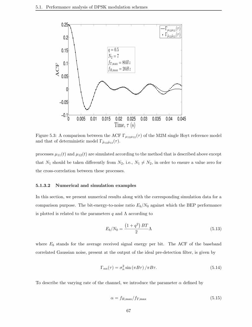
5.1. Performance analysis of DPSK modulation schemes
0 0.005 0.01 0.015 0.02 0.025 0.03 0.035 0.04 0.045−0.1
−0.05
0
0.05
0.1
0.15
0.2
0.25
Time, τ (s)
AC
F
Γµ12µ12(τ)
Γµ12µ12(τ)
q = 0.5N2 = 7fT,max = 80HzfR,max = 20Hz
Figure 5.3: A comparison between the ACF Γµ12µ12(τ) of the M2M single Hoyt reference modeland that of deterministic model Γµ12µ12(τ).
processes µ11(t) and µ12(t) are simulated according to the method that is described above except
that N1 should be taken differently from N2, i.e., N1 6= N2, in order to ensure a value zero for
the cross-correlation between these processes.
5.1.3.2 Numerical and simulation examples
In this section, we present numerical results along with the corresponding simulation data for a
comparison purpose. The bit-energy-to-noise ratio Eb/N0 against which the BEP performance
is plotted is related to the parameters q and Λ according to
Eb/N0 =
(1 + q2
)BT
2Λ (5.13)
where Eb stands for the average received signal energy per bit. The ACF of the baseband
correlated Gaussian noise, present at the output of the ideal pre-detection filter, is given by
Γnn(τ) = σ2n sin (πBτ) /πBτ. (5.14)
To describe the varying rate of the channel, we introduce the parameter α defined by
α = fR,max/fT,max (5.15)
67

5.1. Performance analysis of DPSK modulation schemes
0 10 20 30 40 50 60 70 8010−3
10−2
10−1
100
Eb/N0 (dB)
Average
BE
P,PE
BT = 1.0α = 1fT,max = 20Hz
q = 0.2
q = 0.6 q = 1.0
TheorySimulation
q = 0
Figure 5.4: Theoretical and simulated BEP performance of binary noncoherent DPSK for vari-ous values of the Hoyt fading parameter q.
with 0 ≤ α ≤ 1, assuming fR,max ≤ fT,max. First, we consider the effect of the Hoyt fading
severity parameter q on the BEP performance. The relevant performance is shown in Figure
5.4, where the BEP is depicted as a function of Eb/N0 for BT = 1, fT,max = 20 Hz, α = 1, and
various values of q. The theoretical results are in a good agreement with the simulated ones,
demonstrating, thus, the validity of the theoretical analysis. As expected, the lowest BEP is
obtained for q = 1, i.e., the case of Rayleigh fading channels, while the highest one corresponds
to the one-sided Gaussian channel, i.e., q = 0. It is shown that the BEP performance degrades
with the decreasing values of q. For large values of Eb/N0, an irreducible error floor, caused
by the Doppler spread, appears. Next, the effect of the maximum Doppler frequencies on the
BEP performance is examined. The illustrating curves are plotted in Figure 5.5, for q = 0.6,
BT = 1, fT,max = 80 Hz, and different values of α. In this case, again, the simulated curves
closely match the theoretical curves. The occurrence of the error floor at high values of Eb/N0
can also be noticed from this figure. This error floor increases with the increase of the value
of α. Finally, for the sake of comparison, Figure 5.6 shows the BEP for the M2M Doppler
PSD together with that obtained for the Jake’s Doppler PSD [Jakes 1993], i.e., the Doppler
PSD corresponding to the conventional mobile cellular links. In the illustration, the maximum
Doppler frequency encountered in the cellular radio links (α = 0) is chosen to be equal to the
sum of the maximum Doppler frequencies attributed to the motion of the transmitter and the
68
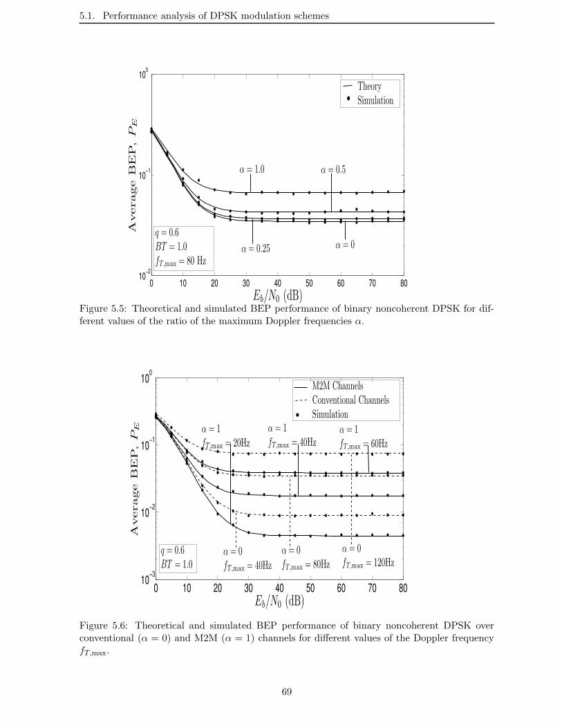
5.1. Performance analysis of DPSK modulation schemes
0 10 20 30 40 50 60 70 8010−2
10−1
100
Eb/N0 (dB)
Average
BE
P,PE
q = 0.6BT = 1.0fT,max = 80 Hz
α = 0.25
TheorySimulation
α = 0
α = 0.5α = 1.0
Figure 5.5: Theoretical and simulated BEP performance of binary noncoherent DPSK for dif-ferent values of the ratio of the maximum Doppler frequencies α.
0 10 20 30 40 50 60 70 8010−3
10−2
10−1
100
Eb/N0 (dB)
Average
BE
P,PE
M2M ChannelsConventional ChannelsSimulation
α = 1fT,max = 20Hz
α = 0fT,max = 40Hz
α = 0fT,max = 80Hz
α = 1fT,max = 40Hz
α = 1fT,max = 60Hz
α = 0fT,max = 120Hz
q = 0.6BT = 1.0
Figure 5.6: Theoretical and simulated BEP performance of binary noncoherent DPSK overconventional (α = 0) and M2M (α = 1) channels for different values of the Doppler frequencyfT,max.
69
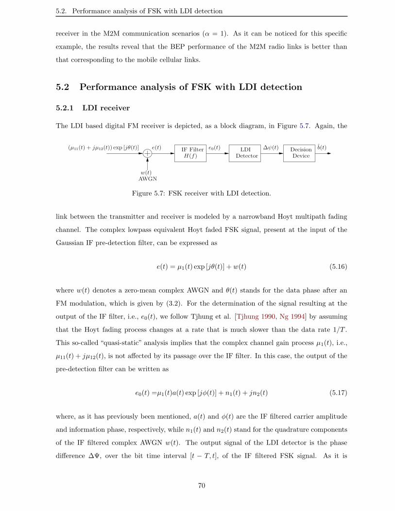
5.2. Performance analysis of FSK with LDI detection
receiver in the M2M communication scenarios (α = 1). As it can be noticed for this specific
example, the results reveal that the BEP performance of the M2M radio links is better than
that corresponding to the mobile cellular links.
5.2 Performance analysis of FSK with LDI detection
5.2.1 LDI receiver
The LDI based digital FM receiver is depicted, as a block diagram, in Figure 5.7. Again, the
b(t)
w(t)AWGN
IF FilterH(f)
e(t)(µ11(t) + jµ12(t)) exp [jθ(t)] e0(t) LDIDetector
DecisionDevice
∆ψ(t)
Figure 5.7: FSK receiver with LDI detection.
link between the transmitter and receiver is modeled by a narrowband Hoyt multipath fading
channel. The complex lowpass equivalent Hoyt faded FSK signal, present at the input of the
Gaussian IF pre-detection filter, can be expressed as
e(t) = µ1(t) exp [jθ(t)] + w(t) (5.16)
where w(t) denotes a zero-mean complex AWGN and θ(t) stands for the data phase after an
FM modulation, which is given by (3.2). For the determination of the signal resulting at the
output of the IF filter, i.e., e0(t), we follow Tjhung et al. [Tjhung 1990, Ng 1994] by assuming
that the Hoyt fading process changes at a rate that is much slower than the data rate 1/T .
This so-called “quasi-static” analysis implies that the complex channel gain process µ1(t), i.e.,
µ11(t) + jµ12(t), is not affected by its passage over the IF filter. In this case, the output of the
pre-detection filter can be written as
e0(t) =µ1(t)a(t) exp [jφ(t)] + n1(t) + jn2(t) (5.17)
where, as it has previously been mentioned, a(t) and φ(t) are the IF filtered carrier amplitude
and information phase, respectively, while n1(t) and n2(t) stand for the quadrature components
of the IF filtered complex AWGN w(t). The output signal of the LDI detector is the phase
difference ∆Ψ, over the bit time interval [t − T, t], of the IF filtered FSK signal. As it is
70
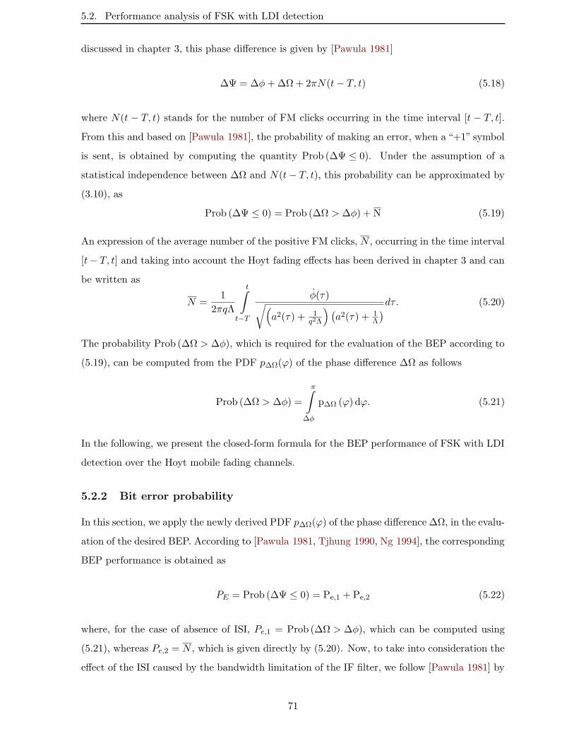
5.2. Performance analysis of FSK with LDI detection
discussed in chapter 3, this phase difference is given by [Pawula 1981]
∆Ψ = ∆φ+∆Ω+ 2πN(t− T, t) (5.18)
where N(t − T, t) stands for the number of FM clicks occurring in the time interval [t − T, t].
From this and based on [Pawula 1981], the probability of making an error, when a “+1” symbol
is sent, is obtained by computing the quantity Prob (∆Ψ ≤ 0). Under the assumption of a
statistical independence between ∆Ω and N(t− T, t), this probability can be approximated by
(3.10), as
Prob (∆Ψ ≤ 0) = Prob (∆Ω > ∆φ) + N (5.19)
An expression of the average number of the positive FM clicks, N , occurring in the time interval
[t− T, t] and taking into account the Hoyt fading effects has been derived in chapter 3 and can
be written as
N =1
2πqΛ
t∫
t−T
φ(τ)√(a2(τ) + 1
q2Λ
) (a2(τ) + 1
Λ
)dτ. (5.20)
The probability Prob (∆Ω > ∆φ), which is required for the evaluation of the BEP according to
(5.19), can be computed from the PDF p∆Ω(ϕ) of the phase difference ∆Ω as follows
Prob (∆Ω > ∆φ) =
π∫
∆φ
p∆Ω (ϕ) dϕ. (5.21)
In the following, we present the closed-form formula for the BEP performance of FSK with LDI
detection over the Hoyt mobile fading channels.
5.2.2 Bit error probability
In this section, we apply the newly derived PDF p∆Ω(ϕ) of the phase difference ∆Ω, in the evalu-
ation of the desired BEP. According to [Pawula 1981, Tjhung 1990, Ng 1994], the corresponding
BEP performance is obtained as
PE = Prob (∆Ψ ≤ 0) = Pe,1 + Pe,2 (5.22)
where, for the case of absence of ISI, Pe,1 = Prob (∆Ω > ∆φ), which can be computed using
(5.21), whereas Pe,2 = N , which is given directly by (5.20). Now, to take into consideration the
effect of the ISI caused by the bandwidth limitation of the IF filter, we follow [Pawula 1981] by
71
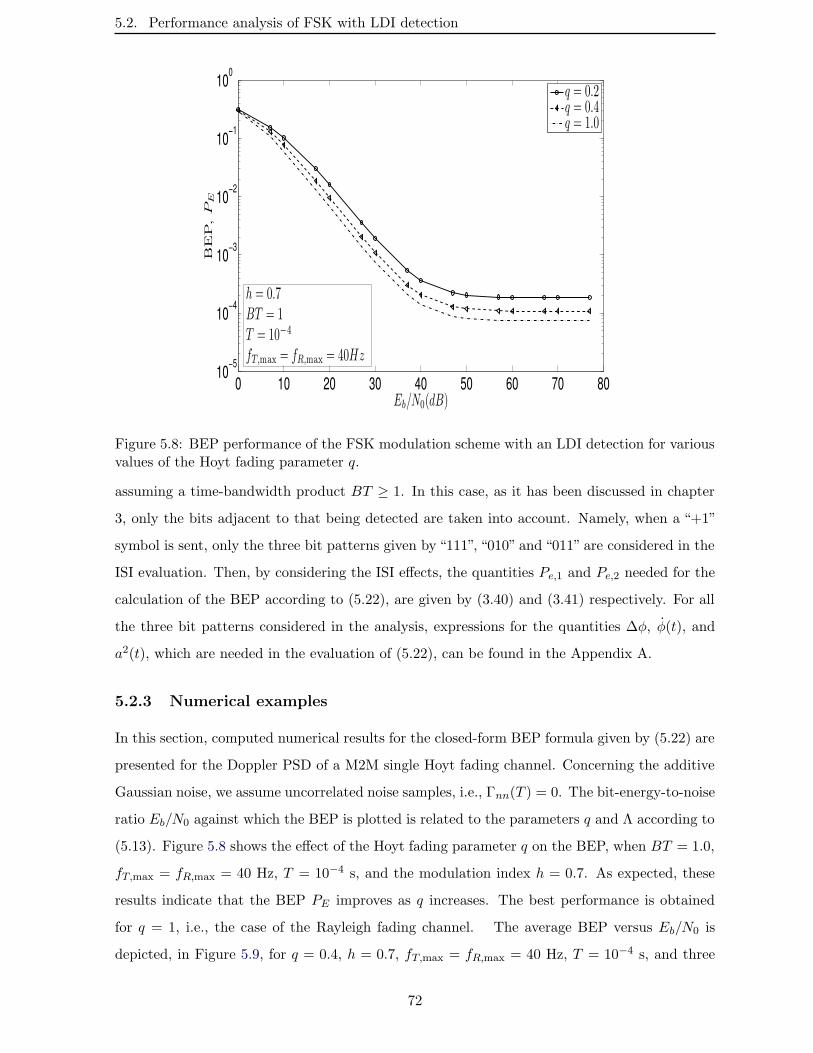
5.2. Performance analysis of FSK with LDI detection
0 10 20 30 40 50 60 70 8010−5
10−4
10−3
10−2
10−1
100
Eb/N0(dB)
BE
P,PE
q = 0.2q = 0.4q = 1.0
h = 0.7BT = 1T = 10−4
fT,max = fR,max = 40Hz
Figure 5.8: BEP performance of the FSK modulation scheme with an LDI detection for variousvalues of the Hoyt fading parameter q.
assuming a time-bandwidth product BT ≥ 1. In this case, as it has been discussed in chapter
3, only the bits adjacent to that being detected are taken into account. Namely, when a “+1”
symbol is sent, only the three bit patterns given by “111”, “010” and “011” are considered in the
ISI evaluation. Then, by considering the ISI effects, the quantities Pe,1 and Pe,2 needed for the
calculation of the BEP according to (5.22), are given by (3.40) and (3.41) respectively. For all
the three bit patterns considered in the analysis, expressions for the quantities ∆φ, φ(t), and
a2(t), which are needed in the evaluation of (5.22), can be found in the Appendix A.
5.2.3 Numerical examples
In this section, computed numerical results for the closed-form BEP formula given by (5.22) are
presented for the Doppler PSD of a M2M single Hoyt fading channel. Concerning the additive
Gaussian noise, we assume uncorrelated noise samples, i.e., Γnn(T ) = 0. The bit-energy-to-noise
ratio Eb/N0 against which the BEP is plotted is related to the parameters q and Λ according to
(5.13). Figure 5.8 shows the effect of the Hoyt fading parameter q on the BEP, when BT = 1.0,
fT,max = fR,max = 40 Hz, T = 10−4 s, and the modulation index h = 0.7. As expected, these
results indicate that the BEP PE improves as q increases. The best performance is obtained
for q = 1, i.e., the case of the Rayleigh fading channel. The average BEP versus Eb/N0 is
depicted, in Figure 5.9, for q = 0.4, h = 0.7, fT,max = fR,max = 40 Hz, T = 10−4 s, and three
72
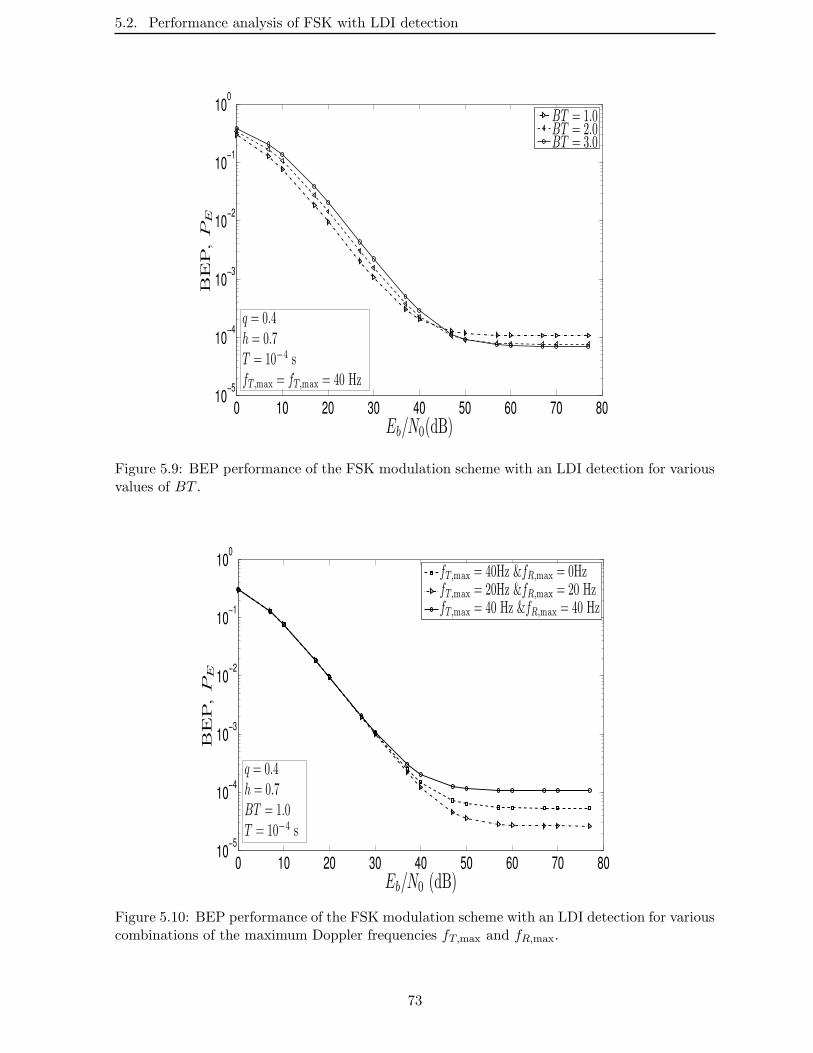
5.2. Performance analysis of FSK with LDI detection
0 10 20 30 40 50 60 70 8010−5
10−4
10−3
10−2
10−1
100
Eb/N0(dB)
BE
P,PE
BT = 1.0BT = 2.0BT = 3.0
q = 0.4h = 0.7T = 10−4 sfT,max = fT,max = 40 Hz
Figure 5.9: BEP performance of the FSK modulation scheme with an LDI detection for variousvalues of BT .
0 10 20 30 40 50 60 70 8010−5
10−4
10−3
10−2
10−1
100
Eb/N0 (dB)
BE
P,PE
fT,max = 40Hz &fR,max = 0HzfT,max = 20Hz &fR,max = 20 HzfT,max = 40 Hz &fR,max = 40 Hz
q = 0.4h = 0.7BT = 1.0T = 10−4 s
Figure 5.10: BEP performance of the FSK modulation scheme with an LDI detection for variouscombinations of the maximum Doppler frequencies fT,max and fR,max.
73
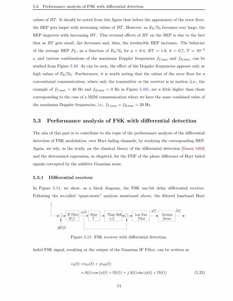
5.3. Performance analysis of FSK with differential detection
values of BT . It should be noted from this figure that before the appearance of the error floor,
the BEP gets larger with increasing values of BT . However, as Eb/N0 becomes very large, the
BEP improves with increasing BT . This reversal effects of BT on the BEP is due to the fact
that as BT gets small, ∆φ decreases and, then, the irreducible BEP increases. The behavior
of the average BEP PE , as a function of Eb/N0 for q = 0.4, BT = 1.0, h = 0.7, T = 10−4
s, and various combinations of the maximum Doppler frequencies fT,max and fR,max, can be
studied from Figure 5.10. As can be seen, the effect of the Doppler frequencies appears only at
high values of Eb/N0. Furthermore, it is worth noting that the values of the error floor for a
conventional communication, where only the transmitter or the receiver is in motion (i.e., the
example of fT,max = 40 Hz and fR,max = 0 Hz in Figure 5.10), are a little higher than those
corresponding to the case of a M2M communication where we have the same combined value of
the maximum Doppler frequencies, i.e., fT,max = fR,max = 20 Hz.
5.3 Performance analysis of FSK with differential detection
The aim of this part is to contribute to the topic of the performance analysis of the differential
detection of FSK modulation, over Hoyt fading channels, by studying the corresponding BEP.
Again, we rely, in the study, on the classical theory of the differential detection [Simon 1983]
and the determined expression, in chapter4, for the PDF of the phase difference of Hoyt faded
signals corrupted by the additive Gaussian noise.
5.3.1 Differential receiver
In Figure 5.11, we show, as a block diagram, the FSK one-bit delay differential receiver.
Following the so-called “quasi-static” analysis mentioned above, the filtered baseband Hoyt
e0(t)
AWGN
y(t) b(t)
FilterLow Pass
DeviceDecisionPhase Shift
π/2DelayTH(f)
IF Filter
Figure 5.11: FSK receiver with differential detection.
faded FSK signal, resulting at the output of the Gaussian IF Filter, can be written as
e0(t) =e01(t) + je02(t)
=A(t) cos (φ(t) + Ω(t)) + jA(t) sin (φ(t) + Ω(t)) (5.23)
74
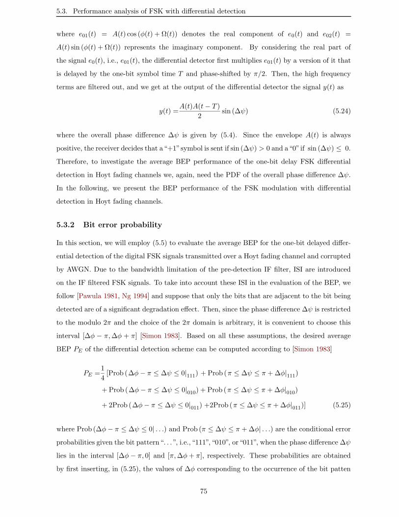
5.3. Performance analysis of FSK with differential detection
where e01(t) = A(t) cos (φ(t) + Ω(t)) denotes the real component of e0(t) and e02(t) =
A(t) sin (φ(t) + Ω(t)) represents the imaginary component. By considering the real part of
the signal e0(t), i.e., e01(t), the differential detector first multiplies e01(t) by a version of it that
is delayed by the one-bit symbol time T and phase-shifted by π/2. Then, the high frequency
terms are filtered out, and we get at the output of the differential detector the signal y(t) as
y(t) =A(t)A(t− T )
2sin (∆ψ) (5.24)
where the overall phase difference ∆ψ is given by (5.4). Since the envelope A(t) is always
positive, the receiver decides that a“+1”symbol is sent if sin (∆ψ) > 0 and a“0”if sin (∆ψ) ≤ 0.
Therefore, to investigate the average BEP performance of the one-bit delay FSK differential
detection in Hoyt fading channels we, again, need the PDF of the overall phase difference ∆ψ.
In the following, we present the BEP performance of the FSK modulation with differential
detection in Hoyt fading channels.
5.3.2 Bit error probability
In this section, we will employ (5.5) to evaluate the average BEP for the one-bit delayed differ-
ential detection of the digital FSK signals transmitted over a Hoyt fading channel and corrupted
by AWGN. Due to the bandwidth limitation of the pre-detection IF filter, ISI are introduced
on the IF filtered FSK signals. To take into account these ISI in the evaluation of the BEP, we
follow [Pawula 1981, Ng 1994] and suppose that only the bits that are adjacent to the bit being
detected are of a significant degradation effect. Then, since the phase difference ∆ψ is restricted
to the modulo 2π and the choice of the 2π domain is arbitrary, it is convenient to choose this
interval [∆φ − π,∆φ + π] [Simon 1983]. Based on all these assumptions, the desired average
BEP PE of the differential detection scheme can be computed according to [Simon 1983]
PE =1
4[Prob (∆φ− π ≤ ∆ψ ≤ 0|111) + Prob (π ≤ ∆ψ ≤ π +∆φ|111)
+ Prob (∆φ− π ≤ ∆ψ ≤ 0|010) + Prob (π ≤ ∆ψ ≤ π +∆φ|010)
+ 2Prob (∆φ− π ≤ ∆ψ ≤ 0|011) +2Prob (π ≤ ∆ψ ≤ π +∆φ|011)] (5.25)
where Prob (∆φ− π ≤ ∆ψ ≤ 0| . . .) and Prob (π ≤ ∆ψ ≤ π +∆φ| . . .) are the conditional error
probabilities given the bit pattern“. . . ”, i.e., “111”, “010”, or“011”, when the phase difference ∆ψ
lies in the interval [∆φ− π, 0] and [π,∆φ+ π], respectively. These probabilities are obtained
by first inserting, in (5.25), the values of ∆φ corresponding to the occurrence of the bit patten
75
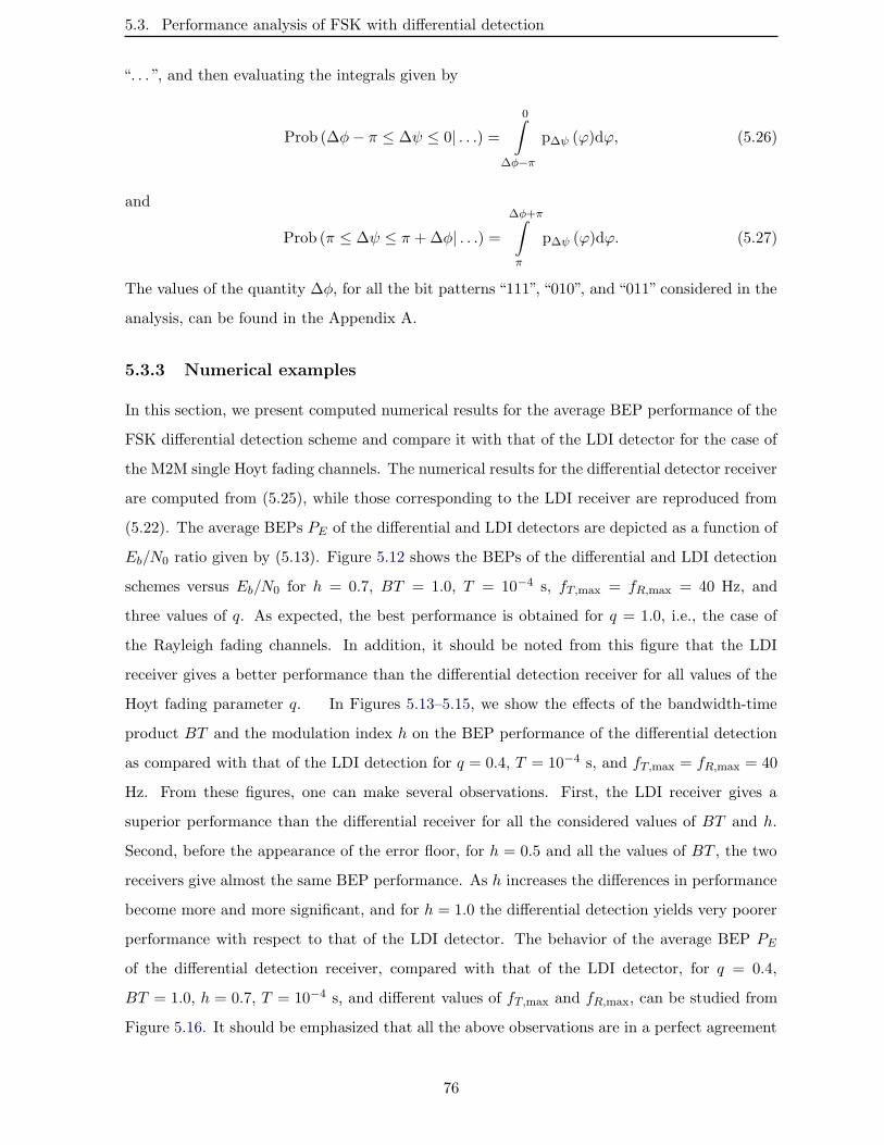
5.3. Performance analysis of FSK with differential detection
“. . . ”, and then evaluating the integrals given by
Prob (∆φ− π ≤ ∆ψ ≤ 0| . . .) =0∫
∆φ−π
p∆ψ (ϕ)dϕ, (5.26)
and
Prob (π ≤ ∆ψ ≤ π +∆φ| . . .) =∆φ+π∫
π
p∆ψ (ϕ)dϕ. (5.27)
The values of the quantity ∆φ, for all the bit patterns “111”, “010”, and “011” considered in the
analysis, can be found in the Appendix A.
5.3.3 Numerical examples
In this section, we present computed numerical results for the average BEP performance of the
FSK differential detection scheme and compare it with that of the LDI detector for the case of
the M2M single Hoyt fading channels. The numerical results for the differential detector receiver
are computed from (5.25), while those corresponding to the LDI receiver are reproduced from
(5.22). The average BEPs PE of the differential and LDI detectors are depicted as a function of
Eb/N0 ratio given by (5.13). Figure 5.12 shows the BEPs of the differential and LDI detection
schemes versus Eb/N0 for h = 0.7, BT = 1.0, T = 10−4 s, fT,max = fR,max = 40 Hz, and
three values of q. As expected, the best performance is obtained for q = 1.0, i.e., the case of
the Rayleigh fading channels. In addition, it should be noted from this figure that the LDI
receiver gives a better performance than the differential detection receiver for all values of the
Hoyt fading parameter q. In Figures 5.13–5.15, we show the effects of the bandwidth-time
product BT and the modulation index h on the BEP performance of the differential detection
as compared with that of the LDI detection for q = 0.4, T = 10−4 s, and fT,max = fR,max = 40
Hz. From these figures, one can make several observations. First, the LDI receiver gives a
superior performance than the differential receiver for all the considered values of BT and h.
Second, before the appearance of the error floor, for h = 0.5 and all the values of BT , the two
receivers give almost the same BEP performance. As h increases the differences in performance
become more and more significant, and for h = 1.0 the differential detection yields very poorer
performance with respect to that of the LDI detector. The behavior of the average BEP PE
of the differential detection receiver, compared with that of the LDI detector, for q = 0.4,
BT = 1.0, h = 0.7, T = 10−4 s, and different values of fT,max and fR,max, can be studied from
Figure 5.16. It should be emphasized that all the above observations are in a perfect agreement
76
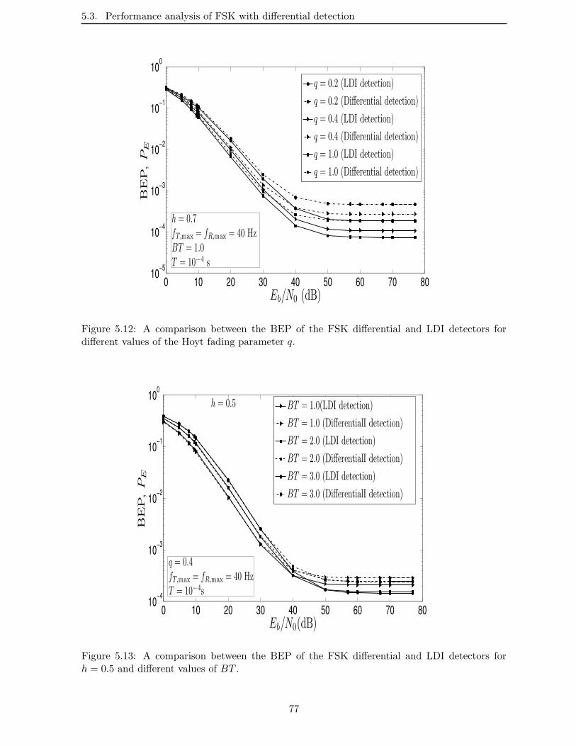
5.3. Performance analysis of FSK with differential detection
0 10 20 30 40 50 60 70 8010−5
10−4
10−3
10−2
10−1
100
Eb/N0 (dB)
BE
P,PE
h = 0.7fT,max = fR,max = 40 HzBT = 1.0T = 10−4 s
q = 0.2 (LDI detection)
q = 0.2 (Differential detection)
q = 0.4 (LDI detection)
q = 0.4 (Differential detection)
q = 1.0 (LDI detection)
q = 1.0 (Differential detection)
Figure 5.12: A comparison between the BEP of the FSK differential and LDI detectors fordifferent values of the Hoyt fading parameter q.
0 10 20 30 40 50 60 70 8010−4
10−3
10−2
10−1
100
Eb/N0(dB)
BE
P,PE
h = 0.5
q = 0.4fT,max = fR,max = 40 HzT = 10−4s
BT = 1.0(LDI detection)
BT = 1.0 (DifferentialI detection)
BT = 2.0 (LDI detection)
BT = 2.0 (DifferentialI detection)
BT = 3.0 (LDI detection)
BT = 3.0 (DifferentialI detection)
Figure 5.13: A comparison between the BEP of the FSK differential and LDI detectors forh = 0.5 and different values of BT .
77
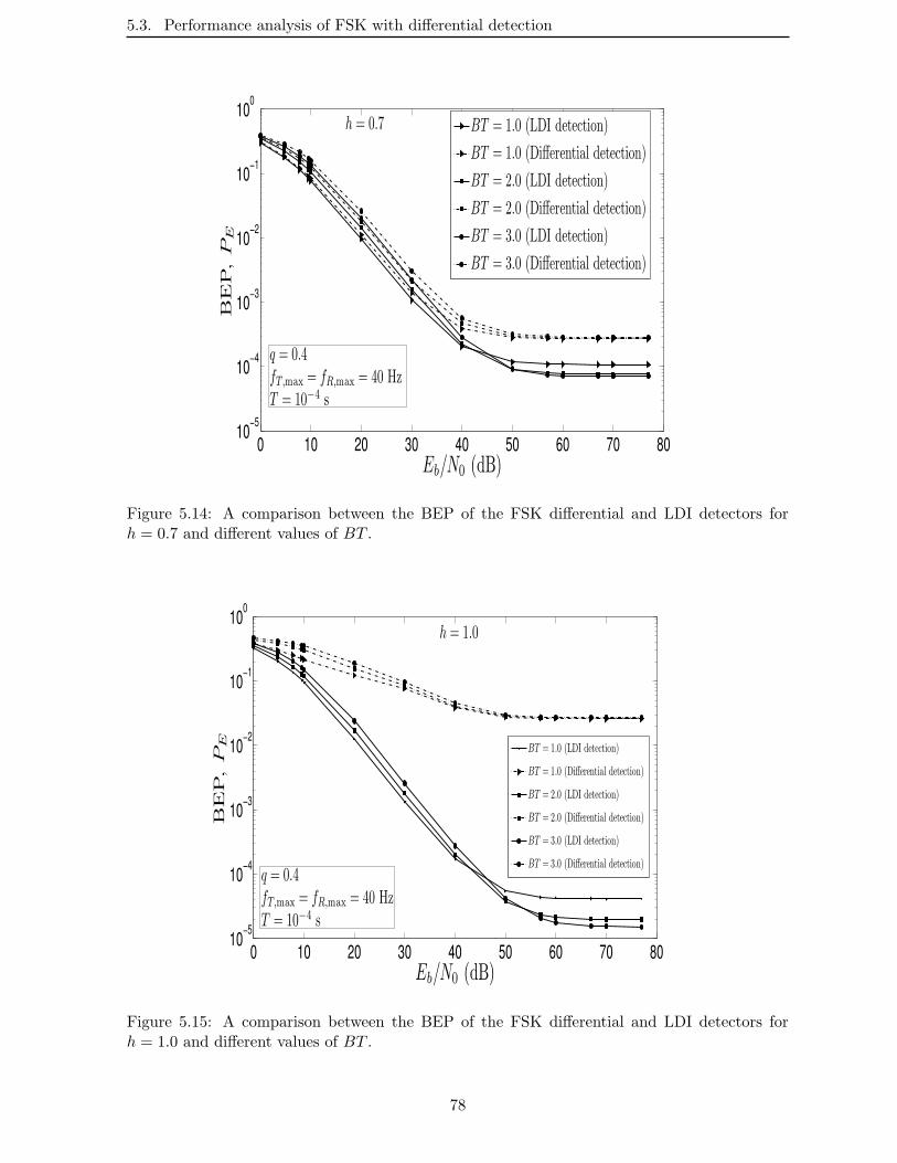
5.3. Performance analysis of FSK with differential detection
0 10 20 30 40 50 60 70 8010−5
10−4
10−3
10−2
10−1
100
Eb/N0 (dB)
BE
P,PE
h = 0.7
q = 0.4fT,max = fR,max = 40 HzT = 10−4 s
BT = 1.0 (LDI detection)
BT = 1.0 (Differential detection)
BT = 2.0 (LDI detection)
BT = 2.0 (Differential detection)
BT = 3.0 (LDI detection)
BT = 3.0 (Differential detection)
Figure 5.14: A comparison between the BEP of the FSK differential and LDI detectors forh = 0.7 and different values of BT .
0 10 20 30 40 50 60 70 8010−5
10−4
10−3
10−2
10−1
100
Eb/N0 (dB)
BE
P,PE
h = 1.0
q = 0.4fT,max = fR,max = 40 HzT = 10−4 s
BT = 1.0 (LDI detection)
BT = 1.0 (Differential detection)
BT = 2.0 (LDI detection)
BT = 2.0 (Differential detection)
BT = 3.0 (LDI detection)
BT = 3.0 (Differential detection)
Figure 5.15: A comparison between the BEP of the FSK differential and LDI detectors forh = 1.0 and different values of BT .
78
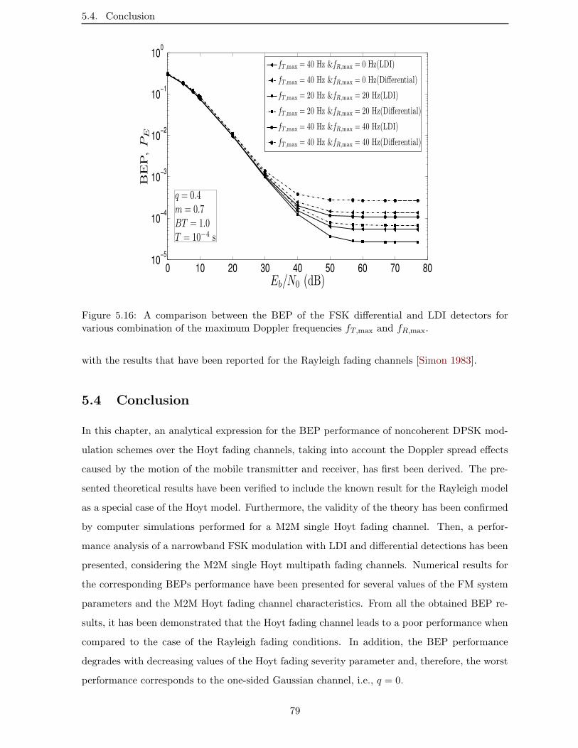
5.4. Conclusion
0 10 20 30 40 50 60 70 8010−5
10−4
10−3
10−2
10−1
100
Eb/N0 (dB)
BE
P,PE
q = 0.4m = 0.7BT = 1.0T = 10−4 s
fT,max = 40 Hz &fR,max = 0 Hz(LDI)
fT,max = 40 Hz &fR,max = 0 Hz(Differential)
fT,max = 20 Hz &fR,max = 20 Hz(LDI)
fT,max = 20 Hz &fR,max = 20 Hz(Differential)
fT,max = 40 Hz &fR,max = 40 Hz(LDI)
fT,max = 40 Hz &fR,max = 40 Hz(Differential)
Figure 5.16: A comparison between the BEP of the FSK differential and LDI detectors forvarious combination of the maximum Doppler frequencies fT,max and fR,max.
with the results that have been reported for the Rayleigh fading channels [Simon 1983].
5.4 Conclusion
In this chapter, an analytical expression for the BEP performance of noncoherent DPSK mod-
ulation schemes over the Hoyt fading channels, taking into account the Doppler spread effects
caused by the motion of the mobile transmitter and receiver, has first been derived. The pre-
sented theoretical results have been verified to include the known result for the Rayleigh model
as a special case of the Hoyt model. Furthermore, the validity of the theory has been confirmed
by computer simulations performed for a M2M single Hoyt fading channel. Then, a perfor-
mance analysis of a narrowband FSK modulation with LDI and differential detections has been
presented, considering the M2M single Hoyt multipath fading channels. Numerical results for
the corresponding BEPs performance have been presented for several values of the FM system
parameters and the M2M Hoyt fading channel characteristics. From all the obtained BEP re-
sults, it has been demonstrated that the Hoyt fading channel leads to a poor performance when
compared to the case of the Rayleigh fading conditions. In addition, the BEP performance
degrades with decreasing values of the Hoyt fading severity parameter and, therefore, the worst
performance corresponds to the one-sided Gaussian channel, i.e., q = 0.
79
5.4. Conclusion
As it has been mentioned in the introduction of this dissertation, in addition to the M2M single
Hoyt fading channels, the double Hoyt fading model can also be used in the statistical descrip-
tion of more realistic M2M propagation environments. Besides, the importance of the double
Hoyt fading, which can be used in the modelling of M2M fading channels where the fading
conditions are worse than those described by the double Rayleigh fading case, there exists no
investigation results on this cascaded channel model so far.
The objective of the next chapter is to contribute to the double Hoyt fading channels by study-
ing and investigating their main statistical properties and their corresponding commonly used
performance measures of wireless communication systems, e.g., frequency of outage and average
outage duration.
80
Chapter 6
Statistical characterization of the
double Hoyt fading channels
Recently and apart from the M2M single fading channels, which are also known as the single
fading double-Doppler channels, attention has been given to the so-called cascaded or double
multipath fading models. Indeed, these fading models, where the overall channel gain between
the transmitter and receiver is obtained as the product of the gains of two statistically in-
dependent fading distributions, have been shown to be more realistic and appropriate in the
description of the direct M2M communications channels, where the transmitter and receiver are
separated by a large distance [Salo 2006b].
Given the importance of double scattering channel distributions in the modeling of M2M
communications, it is a must, therefore, to study and investigate their main statistical prop-
erties, e.g. PDF, CDF, LCR, ADF,.. As is known, the CDF (or equivalently the outage
probability), LCR (or equivalently the frequency of outages), and ADF, which is also known
as the average outage duration, represent the important commonly used performance measures
in the design and performance evaluation of wireless communications systems. In this context,
there are only some few studies available in the literature so far, which are devoted to the
statistical characterization of double fading channels. For instance, the statistical properties
of the double Rayleigh fading channels have been studied in [Patel 2006, Kovacs 2002a]. Re-
cently, in [Talha 2007], analytical expressions for the main statistical properties like the mean
value, variance, PDF, LCR, and ADF of double Rice fading channels have been derived. More
recently, Zlatanov et al. [Zlatanov 2008] derived expressions for the LCR and ADF of double
Nakagami-m fading channels. Theoretical results for the general case of multihop Rayleigh and
Nakagami fading channels, resulting from multiple scattering propagation scenarios, have been
reported in [Karagiannidis 2007, Hadzi-Velkov 2008].
Besides, the importance of the statistical characterization of fading channels, the investi-
gation of the statistical properties of the capacity of time-varying fading channels has been a
subject of intensive research in the recent years. This is mainly due to the potential application
81
6. Statistical characterization of the double Hoyt fading channels
of the capacity statistics in the design and optimization of the modern wireless communication
systems such as those using multiple antennas, adaptive transmission, and user scheduling. In
addition to the mean capacity, considerable attention has been devoted to the study of both
the first and second order statistics. Particularly, the second order statistics in the form of
the ACF, LCR, and ADF provide a deep insight into the dynamical behavior of the capacity
encounters in systems with high mobility applications notably in the case of the inter-vehicular
communications. For instance, the analysis of the outage capacity of double Rayleigh fading
channels has been presented in [Almers 2006, Gesbert 2002]. Recently, Rafiq et al. [Rafiq 2009]
derived expressions for the PDF, CDF, LCR, and ADF of the capacity of double Rice and
double Rayleigh fading channels.
As it has been mentioned, in addition to all the underlying classical fading channel models,
the Hoyt model can also be useful for the description of realistic multipath propagation scenarios
[Nakagami 1960, Youssef 2005b]. In the case of a double fading channel, the corresponding
multipath propagation effects can be modeled by a double Hoyt process. The objective of this
chapter is to investigate the main statistics of the double Hoyt fading channels together with that
of the corresponding channel capacity process. In our analysis, the underlying two single Hoyt
fading processes, leading to the double Hoyt process, are considered as statistically independent,
but not necessarily identically distributed. In this context, we provide theoretical expressions
for the mean value, variance, PDF, LCR, and ADF of the double Hoyt fading processes. In
addition, an expression for the PDF of the phase of the double Hoyt channel is also derived.
Moreover, expressions for the PDF, CDF, LCR, and ADF of the capacity of double Hoyt fading
channels are presented. All the derived quantities include the corresponding known results for
the double Rayleigh fading channel as a special case. In addition, the double fading channels
described by the combinations Rayleigh×Hoyt, Rayleigh×one-sided Gaussian, and double one-
sided Gaussian are special cases of the double Hoyt distribution and, therefore, the results
obtained, in this work, are all valid for these multipath fading channel models. Furthermore,
the validity of the obtained results is demonstrated by computer simulations.
The rest of the chapter is structured as follows. Section 6.1 presents preliminaries and the
formulation of the double Hoyt fading channel. Expressions for the main statistical properties
of the double fading channel are presented in Section 6.2. Namely, analytical expressions for
the mean value, variance, envelope PDF, phase PDF, LCR, and ADF of the corresponding
channel model are derived in this Section. The first and second order statistics in terms of the
PDF, CDF, LCR, and ADF of the channel capacity are investigated in Section 6.3. Numerical
and simulation results of the PDFs, LCR, and ADF expressions for the double Hoyt fading
82
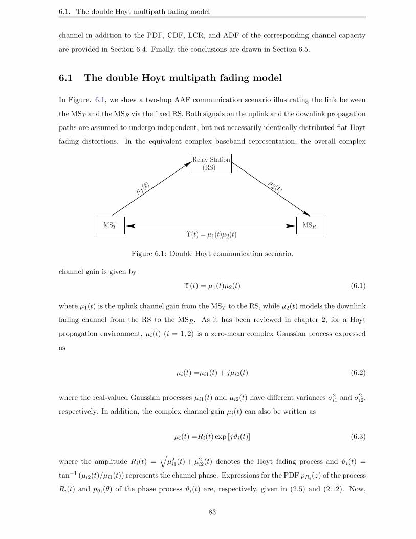
6.1. The double Hoyt multipath fading model
channel in addition to the PDF, CDF, LCR, and ADF of the corresponding channel capacity
are provided in Section 6.4. Finally, the conclusions are drawn in Section 6.5.
6.1 The double Hoyt multipath fading model
In Figure. 6.1, we show a two-hop AAF communication scenario illustrating the link between
the MST and the MSR via the fixed RS. Both signals on the uplink and the downlink propagation
paths are assumed to undergo independent, but not necessarily identically distributed flat Hoyt
fading distortions. In the equivalent complex baseband representation, the overall complex
µ 1(t)
µ2 (t)
(RS)Relay Station
MST MSRΥ(t) = µ1(t)µ2(t)
Figure 6.1: Double Hoyt communication scenario.
channel gain is given by
Υ(t) = µ1(t)µ2(t) (6.1)
where µ1(t) is the uplink channel gain from the MST to the RS, while µ2(t) models the downlink
fading channel from the RS to the MSR. As it has been reviewed in chapter 2, for a Hoyt
propagation environment, µi(t) (i = 1, 2) is a zero-mean complex Gaussian process expressed
as
µi(t) =µi1(t) + jµi2(t) (6.2)
where the real-valued Gaussian processes µi1(t) and µi2(t) have different variances σ2i1 and σ2i2,
respectively. In addition, the complex channel gain µi(t) can also be written as
µi(t) =Ri(t) exp [jϑi(t)] (6.3)
where the amplitude Ri(t) =√µ2i1(t) + µ2i2(t) denotes the Hoyt fading process and ϑi(t) =
tan−1 (µi2(t)/µi1(t)) represents the channel phase. Expressions for the PDF pRi(z) of the process
Ri(t) and pϑi(θ) of the phase process ϑi(t) are, respectively, given in (2.5) and (2.12). Now,
83
6.2. Statistical properties of the fading channel
substituting (6.3) in (6.1), the complex process Υ(t) can be expressed as a function of the
processes R1(t), R2(t), ϑ1(t), and ϑ2(t) according to
Υ(t) = Ξ(t) exp [jΘ(t)] (6.4)
where Ξ(t) = |Υ(t)| = R1(t)R2(t) denotes the double Hoyt process, and Θ(t) = ϑ1(t) + ϑ2(t)
represents the phase process of the double Hoyt fading channel. The aim of the following is to
investigate the main statistical properties of the double Hoyt process Ξ(t) and the phase process
Θ(t).
6.2 Statistical properties of the fading channel
6.2.1 Mean Value and variance
In this section, the mean value and variance of the double Hoyt process Ξ(t) are derived. Since
the Hoyt fading processes R1(t) and R2(t) are considered to be statistically independent, these
statistical quantities can be obtained without the need to resort to the joint PDF of R1(t) and
R2(t). Accordingly, the mean value E Ξ(t) of the double Hoyt process Ξ(t) can be expressed
as
E Ξ(t) = E R1(t)E R2(t) . (6.5)
An expression for the mean value E Ri(t) (i = 1, 2) of the Hoyt fading process Ri(t) can be
determined according to [Papoulis 2002]
E Ri(t) =
∞∫
0
z pRi(z) dz. (6.6)
By substituting (2.5) in (6.6) and using [Gradshteyn 1994, Eqs. 6.621(1) and 8.406(3)], an
expression for E Ri(t) can be obtained as
E Ri(t) =2√π
A1iσiF
(3
4,5
4; 1;
A22i
A21i
), i = 1, 2 (6.7)
where σ2i = σ2i1+σ2i2, F (·) denotes the hypergeometric function [Gradshteyn 1994, Eq. (9.100)],
and the quantities A1i and A2i are given by
A1i =((1 + q2i )/qi
)2, A2i = (1− q4i )/q
2i . (6.8)
84
6.2. Statistical properties of the fading channel
In (6.8), qi (i = 1, 2) stands for the Hoyt fading parameter defined by
qi =σi2σi1
with 0 ≤ qi ≤ 1. (6.9)
Then, substituting (6.7) in (6.5) results in the following expression for the mean value of the
double Hoyt process Ξ(t)
E Ξ(t) =4πσ1σ2A11A12
F
(3
4,5
4; 1;
A221
A211
)F
(3
4,5
4; 1;
A222
A212
). (6.10)
It should be noted that for the special case when q1 = q2 = 1, i.e., the double Rayleigh fading
case, the calculation of the above quantity yields the mean value of the double Rayleigh pro-
cess given by E Ξ(t) = (π/2)σ211 [Kovacs 2002a]. According to [Papoulis 2002], the variance
Var Ξ(t) of the process Ξ(t) can be determined from
Var Ξ(t) = EΞ2(t)
− E Ξ(t)2 (6.11)
where EΞ2(t)
is the mean power of Ξ(t). Again, based on the assumption of the statistical
independence of the processes R1(t) and R2(t), EΞ2(t)
can be written as
EΞ2(t)
= E
R2
1(t)ER2
2(t). (6.12)
Since the mean power of the Hoyt fading process Ri(t) is easily determined to be ER2
i (t)= σ2i ,
the corresponding mean power of the double Hoyt process Ξ(t) is deduced to be
EΞ2(t)
=σ21σ
22. (6.13)
Now, the substitution of (6.10) and (6.13) in (6.11) yields the following expression for the
variance Var Ξ(t) of the double Hoyt fading process Ξ(t)
Var Ξ(t) =σ21σ22
1−
[4π
A11A12F
(3
4,5
4; 1;
A221
A211
)F
(3
4,5
4; 1;
A222
A212
)]2. (6.14)
Again, it should be mentioned that for the special case corresponding to q1 = q2 = 1, the
expression in (6.14) results in the variance of the double Rayleigh fading channel [Kovacs 2002a].
85
6.2. Statistical properties of the fading channel
6.2.2 PDF of the envelope and phase processes
In this section, we present the PDF of the double Hoyt process Ξ(t) and that of the corresponding
phase process Θ(t). Following [Papoulis 2002], the PDF of Ξ(t) can be obtained using
pΞ(z) =
∞∫
−∞
1
|y| pR1R2
(z
y, y
)dy (6.15)
where pR1R2(x, y) is the joint PDF of the envelopes R1(t) and R2(t). Due to the statistical inde-
pendence assumption imposed on the processes R1(t) and R2(t), this joint PDF can be written
as the product of the two marginal PDFs pR1(x) and pR2
(y), i.e., pR1R2(x, y) = pR1
(x) pR2(y).
Hence, the PDF of the double Hoyt process Ξ(t) is given by
pΞ(z) =
√A11A12
σ21σ22
z
∞∫
0
1
yexp
[−A11
4σ21
z2
y2
]exp
[−A12
4σ22y2]I0
[A21
4σ21
z2
y2
]I0
[A22
4σ22y2]dy. (6.16)
Then, the integral in (6.16) must be solved numerically. For the special case corresponding to
the double Rayleigh fading channel, i.e., q1 = q2 = 1, it is found that the integral can be solved
analytically and results in the double Rayleigh distribution, which is known from the study in
[Kovacs 2002a] and is expressed in (2.39). Similarly, for the special case corresponding to the
double one-sided Gaussian fading channel, i.e., q1 → 0 and q2 → 0, (6.16) simplifies to
pΞ(z) =2
πσ11σ22K0
(z
σ11σ22
). (6.17)
In addition, setting q1 = 1 and q2 → 0 in (6.16) and using [Gradshteyn 1994, Eq. 3.472(3)],
then (6.16) becomes
pΞ(z) =1
σ11σ22exp
( −zσ11σ22
)(6.18)
which represents the PDF of the double fading process Ξ(t) corresponding to the Rayleigh×one-
sided Gaussian channel. For completeness, we should add that the PDF described by (6.16) is
valid for the general case where the cascaded single Hoyt fading channels are independent but
not necessarily identically distributed.
The PDF pΘ (θ) of the phase process Θ(t) can be obtained by solving the following integral
[Papoulis 2002]
pΘ (θ) =
∞∫
−∞
pϑ1ϑ2 (θ − ϕ,ϕ) dϕ (6.19)
86
6.2. Statistical properties of the fading channel
where pϑ1ϑ2 (θ1, θ2) is the joint PDF of the phase processes ϑ1(t) and ϑ2(t). Since µ1(t) and
µ2(t) are statistically independent, the phase processes ϑ1(t) and ϑ2(t) are also statistically
independent. Therefore, pϑ1ϑ2 (θ1, θ2) can be written as pϑ1ϑ2 (θ1, θ2) = pϑ1 (θ1) · pϑ2 (θ2). Usingthis result and substituting (2.12) in (6.19), the PDF pΘ (θ) of the phase process Θ(t) for the
double Hoyt channels is obtained to be
pΘ (θ) =q1q2
(2π)2
π∫
−π
1[q21 cos
2 (θ − ϕ) + sin2 (θ − ϕ)] [q22 cos
2 (ϕ) + sin2 (ϕ)]dϕ, −π ≤ θ < π.
(6.20)
It can easily be shown that for the special case given by q1 = q2 = 1, i.e., the double Rayleigh
channel case, the calculation of the above integral yields the PDF of the double Rayleigh model,
i.e., pΘ (θ) = 1/ (2π) , −π ≤ θ < π [Kovacs 2002a].
6.2.3 The LCR and ADF of the fading process
The second order statistics of the double Hoyt fading process Ξ(t), especially the LCR and the
ADF quantities, are presented in this section. The LCR describes how often the process Ξ(t)
crosses a given level r from up to down (or from down to up) per time unit. This quantity
is denoted here by NΞ(r) and can be obtained by solving the following integral [Rice 1944,
Rice 1945]
NΞ(r) =
∞∫
0
z pΞΞ (r, z) dz (6.21)
where pΞΞ (z, z) represents the joint PDF of the double Hoyt process Ξ(t) and its time derivative
Ξ(t) at the same time instant. Following [Patzold 2002], this joint PDF can be computed by
using
pΞΞ (z, z) =
∞∫
0
∞∫
−∞
1
y2pR1R1
(z
y,z
y− z
y2y
)pR2R2
(y, y) dydy z ≥ 0, |z| <∞ (6.22)
where pRiRi(x, x) (i = 1, 2) represents the joint PDF of the Hoyt process Ri(t) and its time
derivative Ri(t). This joint PDF has first been derived in [Youssef 2005b] and has the form
pRiRi(x, x) =
√A1i
(2π)3/2 σ2ix
2π∫
0
exp
[−√A1i
2σ2ix2(q2i cos
2(θ) + sin2(θ))]
× exp
[− x2
2 (βi2 + (βi1 − βi2) cos2(θ))
]× 1√
(βi2 + (βi1 − βi2) cos2(θ))dθ. (6.23)
87
6.2. Statistical properties of the fading channel
In (6.23), the quantities βi1 and βi2 represent the negative curvature of the autocorrelation
function Γµi1µi1(τ) and Γµi2µi2(τ) of the processes µi1(t) and µi2(t), respectively, at τ = 0, i.e.,
βi1 = −Γµi1µi1(0) and βi2 = −Γµi2µi2(0). Now, by substituting (6.23) in (6.22) and with the
help of [Gradshteyn 1994, Eq. 3.323(27)], we get the following expression for the joint PDF
pΞΞ (z, z) of the processes Ξ(t) and Ξ(t)
pΞΞ (z, z) =
√A11A12
(2π)2√2πσ21σ
22
z
2π∫
0
2π∫
0
∞∫
0
1√z2D2 + y4E2
exp
[−√A11
2q1σ21
z2
y2F2
]
× exp
[−√A12
2q2σ22y2G2
]exp
[− (zy)2
2 [z2D2 + y4E2]
]dθ1dθ2dy (6.24)
where the quantities D2, E2, F2, and G2 are given by
D2 =(β22 + (β21 − β22) cos
2(θ2))
E2 =(β12 + (β11 − β12) cos
2(θ1))
F2 =(q21 cos
2(θ1) + sin2(θ1))
G2 =(q22 cos
2(θ2) + sin2(θ2)). (6.25)
Finally, by substituting (6.24) in (6.21) and performing again some algebraic manipulations,
the LCR NΞ(r) of the double Hoyt fading process Ξ(t) can be expressed in the final form as
NΞ(r) =
√A11A12
(2π)2√2πσ21σ
22
r
2π∫
0
2π∫
0
∞∫
0
1
y
√(r
y
)2
D2 + y2E2
× exp
[−√A11
2q1σ21
(r
y
)2
F2
]exp
[−√A12
2q2σ22y2G2
]dθ1dθ2dy. (6.26)
Again, by letting q1 = q2 = 1, the obtained quantity (6.26) reduces to the LCR of the double
Rayleigh process reported in [Patel 2006]. Here, it should be emphasized that NΞ(r) is useful
for studying the frequency of outages, which is a performance measure commonly used in the
wireless communications.
In addition to the LCR, the ADF quantity is of a great importance to the characterization of
the fading channels. The ADF of the double Hoyt process Ξ(t) is denoted here by TΞ−(r). This
quantity represents the expected value for the length of the time intervals during which the
88
6.3. Statistical properties of the channel capacity
process Ξ(t) is below a given level r. Following [Jakes 1993], the ADF TΞ−(r) is defined by
TΞ−(r) =PΞ−(r)
NΞ(r)(6.27)
where PΞ−(r) denotes the CDF of the double Hoyt process Ξ(t) being the probability that Ξ(t)
is below the level r. Using (6.16), an expression for the CDF PΞ−(r) is obtained as
PΞ−(r) =
√A11A12
σ21σ22
∞∫
0
1
yexp
[−A12
4σ22y2]I0
(A21
4σ22y2) r∫
0
z exp
[−A11
4σ21
z2
y2
]I0
[A21
4σ21
z2
y2
]dzdy.
(6.28)
Finally, by substituting (6.26) and (6.28) in (6.27), a formula for the ADF TΞ−(r) of the double
Hoyt process Ξ(t) can be deduced. Also, it can be noted that the CDF, PΞ−(r), and ADF, TΞ−(r)
represent important commonly performance measures used for studying the outage probability
and average duration of fading, respectively, in the wireless communications systems.
6.3 Statistical properties of the channel capacity
The normalized time varying capacity process, which is also known as the instantaneous spec-
tral efficiency, of the double Hoyt fading channels can be expressed using Shannon’s universal
equation [Foschini 1998] as
C(t) = log2(1 + γ Ξ2(t)
)(6.29)
where the process Ξ2(t) represents the channel power gain and the quantity γ denotes the
average SNR. In the following, the statistical properties of the capacity of narrowband double
Hoyt fading channels are studied. Toward this end, analytical expressions for the PDF and CDF
of the instantaneous channel capacity process are derived. Furthermore, for the characterization
of the dynamical behavior of the time-varying channel capacity, expressions are provided for
the LCR and the ADF. Since the double Rayleigh fading channel is a special case of the double
Hoyt model, it is shown that the derived expressions can be reduced to the corresponding results
already known for the capacity of the double Rayleigh fading channel.
89
6.3. Statistical properties of the channel capacity
6.3.1 PDF and CDF of the channel capacity
It can be noted from (6.29) that the capacity C(t) appears as a mapping of the random process
Ξ(t). Thus, analytical expressions for the statistics of the capacity C(t) can, in general, be
derived from those of Ξ(t) reported in previous parts. Specifically, the PDF of the capacity C(t)
of double Hoyt fading channels can be obtained by applying the concept of transformation of
random variables [Papoulis 2002, p. 130]. This yields, by using z = (2c − 1)/γ, the following
relation
pC(c) =2c ln (2)
γpΞ2
(2c − 1
γ
). (6.30)
For the determination of the PDF pΞ2 (z) of the process Ξ2(t), we again apply the concept of
transformation of random variables. As a result, this PDF can be expressed as
pΞ2(z) =1
2√zpΞ(√z). (6.31)
On the assumption that the Hoyt processesR1(t) and R2(t) are statistically independent, we first
substitute (6.16) in (6.31) and then (6.31) in (6.30). Finally, the PDF pC(c) of the instantaneous
capacity C(t) of double Hoyt channels is found to be
pC(c) =2c ln (2)
2γ
√A11A12
σ21σ22
∞∫
0
1
yexp
[− A11
4σ21 γ
2c − 1
y2
]exp
[−A12
4σ22y2]
× I0
[A21
4σ21 γ
2c − 1
y2
]I0
[A22
4σ22y2]dy. (6.32)
The integral involved in (6.32) has to be evaluated by using numerical integration techniques. It
should be mentioned that for the special case q1 = q2 = 1 corresponding to the double Rayleigh
fading channel, (6.32) simplifies to the known result in [Rafiq 2009]
pC(c) =2c ln (2)
2σ411γ
∞∫
0
1
yexp
[− 1
2σ211γ
2c − 1
y2
]exp
[− 1
2σ211y2]dy. (6.33)
The CDF FC(c) of the capacity C(t) of double Hoyt channels can be obtained according to
FC(c) = PC−(c) =
c∫
0
pC(z)dz. (6.34)
90
6.3. Statistical properties of the channel capacity
Substituting (6.32) in (6.34), allows us to obtain the following expression for FC(c)
FC(c) =
√A11A12 ln (2)
2σ21σ22 γ
c∫
0
∞∫
0
2z
yexp
[− A11
4σ21γ
2z − 1
y2
]
× exp
[−A12
4σ22y2]I0
[A21
4σ21 γ
2z − 1
y2
]I0
[A22
4σ22y2]dydz. (6.35)
The integrals in (6.35) can be solved numerically. Again, by setting q1 = q2 = 1, the expression
in (6.35) results in the CDF of the capacity of the double Rayleigh channels given by [Rafiq 2009,
Eq. (18)]. Here, it should be emphasized that FC(c) is useful for studying the outage probability,
which is a performance measure commonly used in wireless communications.
6.3.2 LCR and ADF of the channel capacity
The PDF and CDF derived above do not give any indication concerning the effect of the channel
Doppler spread on the behavior of the instantaneous capacity process. Generally, the study of
this effect requires the knowledge of the LCR and ADF. In this section, we determine expressions
for the LCR and ADF of the capacity C(t) of the double Hoyt channels. Like the LCR NΞ(r) of
double Hoyt fading, the LCR NC(c) of the corresponding channel capacity describes the average
number of up-crossings (or down-crossings) of the capacity through a fixed level within a time
interval of one second. This LCR is defined by [Rice 1944, Rice 1945]
NC(c) =
∞∫
0
cpCC (c, c) dc (6.36)
where pCC (c, c) represents the joint PDF of the processes C(t) and its time derivative C(t).
Thus, in order to find the LCR of the capacity of double Hoyt fading channels, the ex-
pression for this joint PDF is required. From the transformation of random variables us-
ing z = (2c − 1)/γ, z = (2cc ln (2))/γ, and with the corresponding Jacobian determinant
J = (2c ln (2)/γ)2, the joint PDF pCC (c, c) can be written as
pCC (c, c) =
(2c ln (2)
γ
)2
pΞ2Ξ2
(2c − 1
γ,2cc ln (2)
γ
)(6.37)
where pΞ2Ξ2 (z, z) stands for the joint PDF of the processes Ξ2(t) and its time derivative Ξ2(t).
Based upon the transformation of random variables x =√z, x = z/(2
√z), and with the cor-
responding Jacobian determinant given by J = 1/(4z), this joint PDF can be expressed as a
91
6.3. Statistical properties of the channel capacity
function of the joint PDF pΞΞ (z, z) of the processes Ξ(t) and Ξ(t) according to
pΞ2Ξ2(z, z) =1
4zpΞΞ
(√z,
z
2√z
). (6.38)
Now, substituting the joint PDF pΞΞ (z, z), as presented in (6.24), in (6.38) and carrying out
some algebraic manipulations, the joint PDF pΞ2Ξ2(z, z) of the process Ξ2(t) and its time deriva-
tive Ξ2(t) is found to be
pΞ2Ξ2 (z, z) =
√A11A12
(4π)2√2πσ21σ
22
√z
2π∫
0
2π∫
0
∞∫
0
1√zD2 + y4E2
exp
[−√A11
2q1σ21
z
y2F2
]
× exp
[−√A12
2q2σ22y2G2
]exp
[− (zy)2
8z [zD2 + y4E2]
]dθ1dθ2 dy. (6.39)
Then, by substituting (6.39) in (6.37), we obtain the following expression for the joint PDF
pCC (c, c)
pCC (c, c) =
√A11A12
(4π)2√2πσ21σ
22
√γ
2c − 1
(2c ln (2)
γ
)22π∫
0
2π∫
0
∞∫
0
1√(2c−1γ
)D2 + y4E2
× exp
[− (2cc ln (2) y)2
8 (2c − 1) [(2c − 1)D2 + y4γE2]
]exp
[−
√A11
2q1σ21y2
(2c − 1
γ
)F2
]
× exp
[−√A12
2q2σ22y2G2
]dθ1dθ2 dy. (6.40)
Finally, after substituting (6.40) into (6.36) and carrying out some algebraic manipulations, we
get the desired LCR NC(c) as
NC(c) =
√A11A12
(2π)5/2 σ21σ22
√2c − 1
γ
2π∫
0
2π∫
0
∞∫
0
√(2c − 1
γy4
)D2 + E2
× exp
[−
√A11
2q1σ21y2
(2c − 1
γ
)F2
]exp
[−√A12
2q2σ22y2G2
]dθ1dθ2 dy. (6.41)
The integrals in (6.41) have to be solved numerically. It should be noted that for the double
Rayleigh fading channel, i.e., q1 = q2 = 1, it is found that the threefold integral in (6.41) can
be reduced to a single integral and results in the LCR of the double Rayleigh fading channels,
92
6.4. Numerical and simulation results
which is known from the study in [Rafiq 2009], as
NC (c) =
√2c − 1√2πγσ411
∞∫
0
√β12 + β11
(2c − 1
γy4
)exp
[− 1
2σ211y2
(2c − 1
γ
)]exp
[− y2
2σ211
]dy. (6.42)
It is worth mentioning that the derived expression (6.41) for the LCR of the channel capacity
could as well be obtained directly from the LCR NΞ(r) of the envelope of double Hoyt fading
channels given in (6.26) by just replacing the crossing level r by its equivalent quantity in terms
of the capacity r =√(2c − 1)/γ, i.e.,
NC(c) = NΞ
(√(2c − 1)/γ
). (6.43)
More much details on the demonstration of this result can be found in the Appendix C.
The ADF TC (c) of the instantaneous capacity C(t) represents the expected value of the time
intervals during which the capacity C(t) is below at a given level c. Thus, using (6.35) and
(6.41), the ADF TC (c) can be deduced according to [Rice 1944, Rice 1945]
TC (c) =FC (c)
NC (c). (6.44)
6.4 Numerical and simulation results
In this section, we present computed numerical results for the derived quantities pΞ(z), pΘ (θ),
NΞ(r), and TΞ−(r) of the double Hoyt fading channels together with pC(c), FC(c), NC(c), and
TC(c) of the corresponding channel capacity process C(t). In addition, we compare all these
results with simulations to confirm the correctness of the theory. In order to simulate the
statistical properties of the processes Ξ(t), Θ(t), and C(t), we use the concept of Rice’s sum-
of-sinusoids [Rice 1944, Rice 1945]. According to that principle, the statistics of the Gaussian
process µij(t) (i, j = 1, 2) can be approximated by the deterministic process µij(t) having the
form
µij(t) =
Nij∑
n=1
cij,n cos (2πfij,nt+ θij,n), i, j = 1, 2 (6.45)
where cij,n, fij,n, and θij,n are the gains, discrete Doppler frequencies, and phases, respectively.
The quantity Nij in (6.45) denotes the number of sinusoids used for the generation of the
deterministic process µij(t). In Figure 6.2, we show the general structure of the deterministic
simulation process µij(t) in its continuous-time representation. For the computation of the
model parameters, we use the so-called MEDS method [Patzold 2002, Hajri 2005]. This method
93
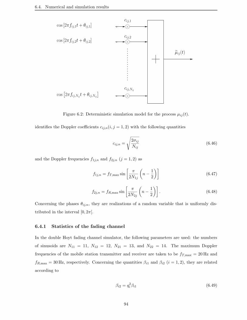
6.4. Numerical and simulation results
cij,2
µij(t)
cij,Nij
cos[2πfij,Nij
t + θij,Nij
]
cos [2πfij,2t + θij,2]
cos [2πfij,1t + θij,1]cij,1
Figure 6.2: Deterministic simulation model for the process µij(t).
identifies the Doppler coefficients cij,n(i, j = 1, 2) with the following quantities
cij,n =
√2σijNij
(6.46)
and the Doppler frequencies f1j,n and f2j,n (j = 1, 2) as
f1j,n = fT,max sin
[π
2N1j
(n− 1
2
)](6.47)
f2j,n = fR,max sin
[π
2N2j
(n− 1
2
)]. (6.48)
Concerning the phases θij,n, they are realizations of a random variable that is uniformly dis-
tributed in the interval [0, 2π[.
6.4.1 Statistics of the fading channel
In the double Hoyt fading channel simulator, the following parameters are used: the numbers
of sinusoids are N11 = 11, N12 = 12, N21 = 13, and N22 = 14. The maximum Doppler
frequencies of the mobile station transmitter and receiver are taken to be fT,max = 20Hz and
fR,max = 30Hz, respectively. Concerning the quantities βi1 and βi2 (i = 1, 2), they are related
according to
βi2 = q2i βi1 (6.49)
94
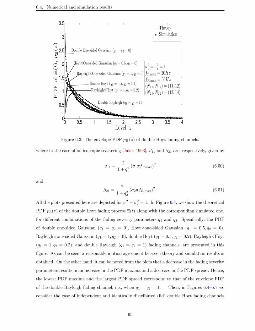
6.4. Numerical and simulation results
0 0.5 1 1.5 2 2.5 3 3.5 40
0.5
1
1.5
2
2.5
3
3.5
Level, z
PD
Fof
Ξ(t)
,p
Ξ(z)
Rayleigh×One-sided Gaussian (q1 = 1, q2 = 0)
Rayleigh×Hoyt (q1 = 1, q2 = 0.2)
Double Hoyt (q1 = 0.5, q2 = 0.2)
Double Rayleigh (q1 = q2 = 1)
Hoyt×One-sided Gaussian (q1 = 0.5, q2 = 0)
Double One-sided Gaussian (q1 = q2 = 0)
TheorySimulation
σ21 = σ2
2 = 1fT,max = 20HzfR,max = 30Hz(N11, N12) = (11, 12)(N21, N22) = (13, 14)
Figure 6.3: The envelope PDF pΞ (z) of double Hoyt fading channels.
where in the case of an isotropic scattering [Jakes 1993], β11 and β21 are, respectively, given by
β11 =2
1 + q21(σ1πfT,max)
2 (6.50)
and
β21 =2
1 + q22(σ2πfR,max)
2 . (6.51)
All the plots presented here are depicted for σ21 = σ22 = 1. In Figure 6.3, we show the theoretical
PDF pΞ(z) of the double Hoyt fading process Ξ(t) along with the corresponding simulated one,
for different combinations of the fading severity parameters q1 and q2. Specifically, the PDF
of double one-sided Gaussian (q1 = q2 = 0), Hoyt×one-sided Gaussian (q1 = 0.5, q2 = 0),
Rayleigh×one-sided Gaussian (q1 = 1, q2 = 0), double Hoyt (q1 = 0.5, q2 = 0.2), Rayleigh×Hoyt
(q1 = 1, q2 = 0.2), and double Rayleigh (q1 = q2 = 1) fading channels, are presented in this
figure. As can be seen, a reasonable mutual agreement between theory and simulation results is
obtained. On the other hand, it can be noted from the plots that a decrease in the fading severity
parameters results in an increase in the PDF maxima and a decrease in the PDF spread. Hence,
the lowest PDF maxima and the largest PDF spread correspond to that of the envelope PDF
of the double Rayleigh fading channel, i.e., when q1 = q2 = 1. Then, in Figures 6.4–6.7 we
consider the case of independent and identically distributed (iid) double Hoyt fading channels
95
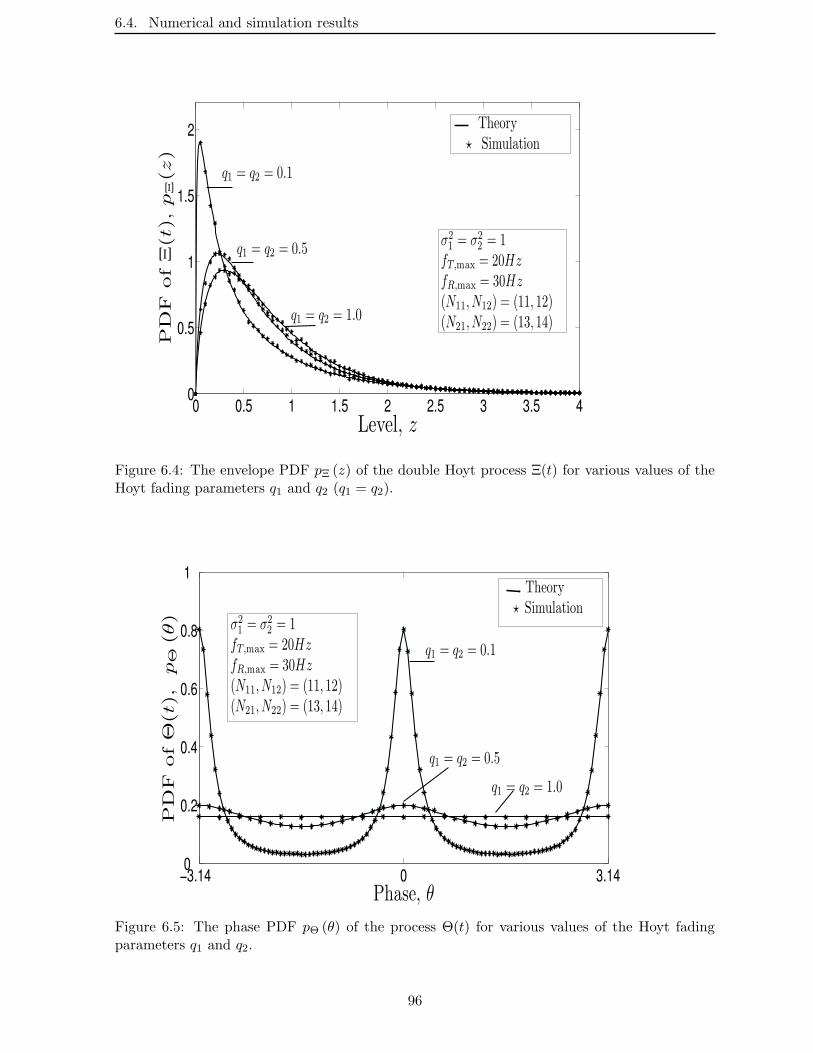
6.4. Numerical and simulation results
0 0.5 1 1.5 2 2.5 3 3.5 40
0.5
1
1.5
2
Level, z
PD
Fof
Ξ(t),p
Ξ(z)
q1 = q2 = 0.1
q1 = q2 = 0.5
q1 = q2 = 1.0
Theory? Simulation
σ21 = σ2
2 = 1fT,max = 20HzfR,max = 30Hz(N11, N12) = (11, 12)(N21, N22) = (13, 14)
Figure 6.4: The envelope PDF pΞ (z) of the double Hoyt process Ξ(t) for various values of theHoyt fading parameters q1 and q2 (q1 = q2).
−3.14 0 3.140
0.2
0.4
0.6
0.8
1
Phase, θ
PD
Fof
Θ(t),p
Θ(θ)
Theory? Simulation
q1 = q2 = 0.1
q1 = q2 = 0.5
q1 = q2 = 1.0
σ21 = σ2
2 = 1fT,max = 20HzfR,max = 30Hz(N11, N12) = (11, 12)(N21, N22) = (13, 14)
Figure 6.5: The phase PDF pΘ (θ) of the process Θ(t) for various values of the Hoyt fadingparameters q1 and q2.
96
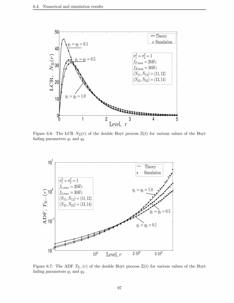
6.4. Numerical and simulation results
0 1 2 3 4 50
10
20
30
40
50
Level, r
LC
R,N
Ξ(r)
q1 = q2 = 0.1
q1 = q2 = 0.5
q1 = q2 = 1.0
Theory? Simulation
σ21 = σ2
2 = 1fT,max = 20HzfR,max = 30Hz(N11, N12) = (11, 12)(N21, N22) = (13, 14)
Figure 6.6: The LCR NΞ(r) of the double Hoyt process Ξ(t) for various values of the Hoytfading parameters q1 and q2.
10−2
10−1
100
101
Level, r
AD
F,T
Ξ−
(r)
Theory? Simulation
σ21 = σ2
2 = 1f1,max = 20Hzf2,max = 30Hz(N11, N12) = (11, 12)(N21, N22) = (13, 14)
q1 = q2 = 0.1
q1 = q2 = 0.5
q1 = q2 = 1.0
2·100 3·100100
Figure 6.7: The ADF TΞ−(r) of the double Hoyt process Ξ(t) for various values of the Hoytfading parameters q1 and q2.
97
6.4. Numerical and simulation results
which are obtained by setting q1 = q2. In this case, Figure 6.4 shows the theoretical PDF pΞ(z)
of the double Hoyt fading process Ξ(t), along with the corresponding PDF deduced from the
simulation of the channel’s envelope, for different values of the Hoyt fading parameters q1 and
q2 with q1 = q2. Again, a reasonable mutual agreement between theory and simulation can
be noted from this figure. Furthermore as expected, the envelope PDF of the double Rayleigh
fading channel, i.e., when q1 = q2 = 1, presents the lowest PDF maxima and the largest PDF
spread. A comparison between the analytical phase PDF pΘ (θ) and that obtained by simulation
is presented in Figure 6.5 for different values of q1 and q2. As can be seen, an excellent fitting
between analytical and simulation results is obtained. In Figure 6.6, we compare the analytical
LCR NΞ(r) of the double Hoyt process Ξ(t) against the corresponding simulation data. First, it
can be observed that theory and simulation results are in accordance with each other. Second,
it can be seen that the LCR maxima and the LCR spread increase with the decrease and the
increase of the Hoyt fading parameters q1 and q2 (q1 = q2), respectively. Therefore, the LCR
with the lowest maxima and the largest spread is obtained for the double Rayleigh fading model,
i.e., q1 = q2 = 1. The excellent fitting between the theoretical and simulation ADF TΞ−(r) of
the double Hoyt channel can be studied from Figure 6.7.
6.4.2 Statistics of the channel capacity
For the simulation of the channel capacity, we consider the same specified values for the simu-
lation parameters as mentioned above. In addition, the SNR is set to γ = 30 dB. A comparison
between the theoretical PDF pC(c) of the channel capacity C(t) and the corresponding simu-
lated one is provided in Figure 6.8 for different values of the Hoyt fading parameters q1 and q2.
As it can be seen, there is an excellent fitting between the theoretical and simulation results.
In addition, this figure shows that the values of q1 and q2 have a significant influence on the
PDF of the capacity of the double Hoyt channels. Specifically, with an increase of q1 and q2,
the maximum value of pC(c) increases, while the spread is seen to decrease. Hence, as expected,
the highest capacity can be achieved if q1 = q2 = 1 corresponding to the double Rayleigh
fading channels. The analytical CDF FC(c) of the channel capacity is shown in Figure 6.9
in comparison with that obtained from computer simulations for different values of q1 and q2.
Also in this case, an excellent agreement between theory and simulation can be observed. As
expected, the outage performance deteriorates with a decrease in the fading severity parameters
q1 and q2. In Figure 6.10, we study the influence of the parameters q1 and q2 on the LCR of
the channel capacity. Again, the simulation results are seen to be in a very good agreement
with the analytical ones. For the range of small values of the capacity level c, which is of a
98
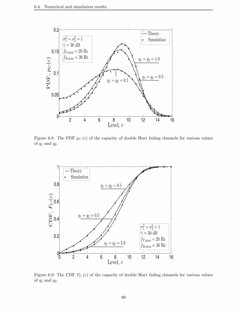
6.4. Numerical and simulation results
2 4 6 8 10 12 14 160
0.05
0.1
0.15
0.2
Level, c
PD
F,pC
(c)
Theory? Simulationσ2
1 = σ22 = 1
γ = 30 dBfT,max = 20 HzfR,max = 30 Hz
q1 = q2 = 0.1
q1 = q2 = 1.0
q1 = q2 = 0.5
Figure 6.8: The PDF pC (c) of the capacity of double Hoyt fading channels for various valuesof q1 and q2.
0 2 4 6 8 10 12 14 160
0.2
0.4
0.6
0.8
1
Level, c
CD
F,FC
(c)
q1 = q2 = 1.0
Theory? Simulation
q1 = q2 = 0.5
q1 = q2 = 0.1
σ21 = σ2
2 = 1γ = 30 dBfT,max = 20 HzfR,max = 30 Hz
Figure 6.9: The CDF FC (c) of the capacity of double Hoyt fading channels for various valuesof q1 and q2.
99
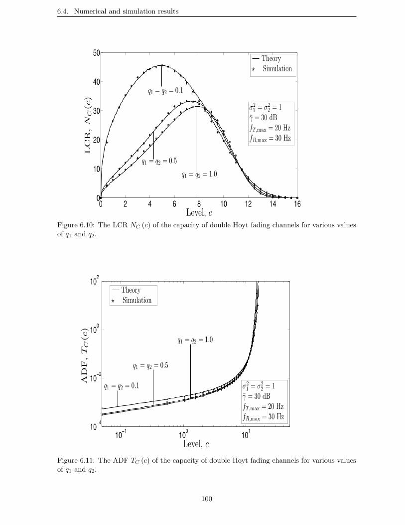
6.4. Numerical and simulation results
0 2 4 6 8 10 12 14 160
10
20
30
40
50
Level, c
LC
R,NC
(c)
Theory? Simulation
q1 = q2 = 0.1
σ21 = σ2
2 = 1γ = 30 dBfT,max = 20 HzfR,max = 30 Hz
q1 = q2 = 1.0
q1 = q2 = 0.5
Figure 6.10: The LCR NC (c) of the capacity of double Hoyt fading channels for various valuesof q1 and q2.
10−1 100 10110−4
10−2
100
102
Level, c
AD
F,TC
(c)
σ21 = σ2
2 = 1γ = 30 dBfT,max = 20 HzfR,max = 30 Hz
Theory? Simulation
q1 = q2 = 1.0
q1 = q2 = 0.5
q1 = q2 = 0.1
Figure 6.11: The ADF TC (c) of the capacity of double Hoyt fading channels for various valuesof q1 and q2.
100
6.5. Conclusions
practical interest, the LCR increases significantly with a decrease of q1 and q2. For high values
of c, however, the impact of these parameters on the LCR is much less pronounced. Finally, a
comparison between the theoretical ADF TC(c) and that obtained from simulations is provided
by Figure 6.11 for different values of q1 and q2. Again, it can be observed that there exists a
reasonable correspondence between theory and simulation. For low values of c, the ADF de-
creases as the fading severity parameters are increased, meaning that the performance in terms
of the average outage duration improves. For completeness, it is worthwhile to mention that
we do not observe any significant change in the behavior of the second order statistics of the
capacity processes compared to those of the envelope of the double Hoyt fading channels, which
have been reported in the previous sections. This is attributed to the fact that the capacity is
a monotonic function of the fading channel power gain.
6.5 Conclusions
In this chapter, a study on the statistical properties of the double Hoyt fading channels and
their corresponding channel capacity process has been presented. First, analytical expressions
for the mean value, variance, PDF, LCR, and ADF of the double Hoyt process have been
derived. Then, an expression for the PDF of the channel phase has been provided. Moreover,
analytical expressions for the PDF, CDF, LCR, and ADF of the channel capacity have been
derived. All the obtained analytical expressions include known results corresponding to the
double Rayleigh fading channel as a special case. Additionally, the validity of the derived
expressions has been confirmed by computer simulations. As it has been mentioned, the CDF,
LCR, and ADF measures are of a crucial importance in the design and performance evaluation
of wireless communication systems.
Besides all these investigated performance measures, the BEP represents the more appropriate
performance measure revealing the nature of the system behavior. Accordingly, it is a must
and of a great interest to study and analyze the BEP performance of M2M communications
over double Hoyt fading channels. In this context and drawing upon the obtained envelope
PDF of the double Hoyt fading channels, the next chapter aims at contributing to the topic
of performance analysis of various digital modulation schemes over the double Hoyt channels
perturbed by AWGN.
101
Chapter 7
BEP of M2M communications over
the double Hoyt fading channels
The present chapter aims at contributing to the performance analysis of M2M communications
over the double Hoyt fading channels, by studying the BEP of several modulation schemes
commonly used in wireless communications.
Namely, we investigate here the impact of the frequency-flat double Hoyt propagation en-
vironments on the error rate performance of coherent BPSK, QPSK, FSK, MSK, and ASK
modulation schemes. Starting from the envelope PDF of the double Hoyt fading channels,
which has been derived in chapter 6, we first give an analytical expression for the PDF of
the receiver output SNR. Then, using this PDF and drawing upon the theory reported in
[Simon 2005, Proakis 2001], an analytical expression, involving a double (definite and semi-
infinite) integral, is presented for the BEP of all the modulation techniques mentioned above.
The obtained formula is generic and includes, as special cases, the BEP corresponding to the dou-
ble one-sided Gaussian, Rayleigh×one-sided Gaussian, Rayleigh×Hoyt, Hoyt×one-sided Gaus-
sian, and double Rayleigh fading channel models. For most of these special cases, the BEP
formula is shown to simplify to closed-form expressions which involve a single integral with
finite limits. The Rayleigh×Hoyt propagation environment can as well be encountered in satel-
lite based mobile communications where the ionospheric scintillation is known to be described
by the Hoyt distribution [Chytil 1967], while the terrestrial multipath fading is characterized
by the Rayleigh channel model. Numerical examples are presented to analyze the behavior of
the BEP for various cases of the fading environments. Moreover, the validity of the analytical
results is demonstrated by using computer simulations for the BPSK modulation scheme.
The remainder of the chapter is organized as follows. In Section 7.1, we first present pre-
liminaries and then derive the PDF of the instantaneous SNR. The average BEP of coherent
modulation schemes previously mentioned, i.e., BPSK, QPSK, FSK, MSK, and ASK, is inves-
tigated in Section 7.2. Numerical results and analysis are provided in Section 7.3, while the
conclusion is drawn in Section 7.4.
102
7.1. The SNR distribution
7.1 The SNR distribution
We consider a radio link between a single-input single-output mobile transmitter and receiver.
The propagation conditions between the two mobiles are modeled statistically by a double Hoyt
fading distribution. By assuming a frequency non-selective fading, the complex valued equiva-
lent baseband signal, present at the input of the mobile receiver, can be written as [Simon 2005]
y(t) = Ξ(t)x(t)ejΘ(t) + n(t) (7.1)
where x(t) is the modulated signal and n(t) represents the complex AWGN with a one-sided
power spectral density N0. As it has been demonstrated in chapter 6, the PDF of the double
Hoyt process Ξ(t) is expressed by (6.16). This PDF expression can also be written as
pΞ(z) =
(1 + q21
) (1 + q22
)
q1q2σ21σ22
z
∞∫
0
1
yexp
[−(1 + q21
)2
4q21σ21
z2
y2
]exp
[−(1 + q22
)2
4q22σ22
y2
]
× I0
[(1− q41
)
4q21σ21
z2
y2
]I0
[(1− q42
)
4q22σ22
y2
]dy. (7.2)
As it is well known, the determination of the average BEP requires the knowledge of the dis-
tribution of the instantaneous SNR per bit. The instantaneous output SNR per bit is defined
as
γs(t) = Ξ2(t)EbN0
(7.3)
where Eb is the average received bit energy. Now, based on the concept of transformation of
random variables [Papoulis 2002, p. 130], the PDF of the instantaneous SNR γs(t) is easily
obtained from (7.3) combined with (7.2) according to
pγs(β) =1
2√β (Eb/N0)
pΞ
(√β
Eb/N0
). (7.4)
Hence, substituting (7.2) in (7.4) yields the following expression for pγs(β)
pγs(β) =
(1 + q21
) (1 + q22
)
2q1q2γs
∞∫
0
1
yexp
[− 1 + q224q22σ
221
y2]exp
[−(1 + q21
)2 (1 + q22
)σ221
4q21y2
β
γs
]
× I0
[1− q224q22σ
221
y2]I0
[(1− q41
) (1 + q22
)σ221
4q21y2
β
γs
]dy (7.5)
103
7.2. BEP derivation
where γs is the average SNR given by
γs = σ21σ22
EbN0
. (7.6)
The integral involved in (7.5) can then be evaluated by using numerical techniques. However,
for the following special cases, the integration can be carried out to yield a closed-form solution
for the PDF of γs(t). Namely, in the case of q1 = q2 = 1, i.e., the case of the double Rayleigh
fading model, the integral can be solved with the help of [Gradshteyn 1994, Eq. 8.432(6.7)].
This yields
pγs(β) =2
γsK0
(2
√β
γs
)(7.7)
Similarly, for the special case corresponding to the double one-sided Gaussian fading channel,
i.e., q1 → 0 and q2 → 0, (7.5) simplifies to
pγs(β) =1
π√βγs
K0
(√β
γs
). (7.8)
In addition, letting q1 = 1 and q2 → 0 in (7.5) and using [Gradshteyn 1994, Eq. 3.472(3)], then
(7.5) becomes
pγs(β) =1√2βγs
exp
(−√
2β
γs
)(7.9)
which is the PDF of the instantaneous SNR corresponding to the Rayleigh×one-sided Gaussian
channel.
For completeness, we should add that the PDF described by (7.5) is valid for the general case
where the cascaded single Hoyt fading channels are independent but not necessarily identically
distributed. Here, it can be observed from (7.5) that the distribution type remains unchanged
regardless of whether the cascaded fading models have identical or non-identical distributions;
except that the statistical parameters are different.
7.2 BEP derivation
For the derivation of the desired BEP, we apply the approach based on the average calculation
of the conditional BEP in an AWGN channel over the instantaneous SNR distribution. That is,
the evaluation of the average BEP performance can be accomplished according to [Simon 2005,
104
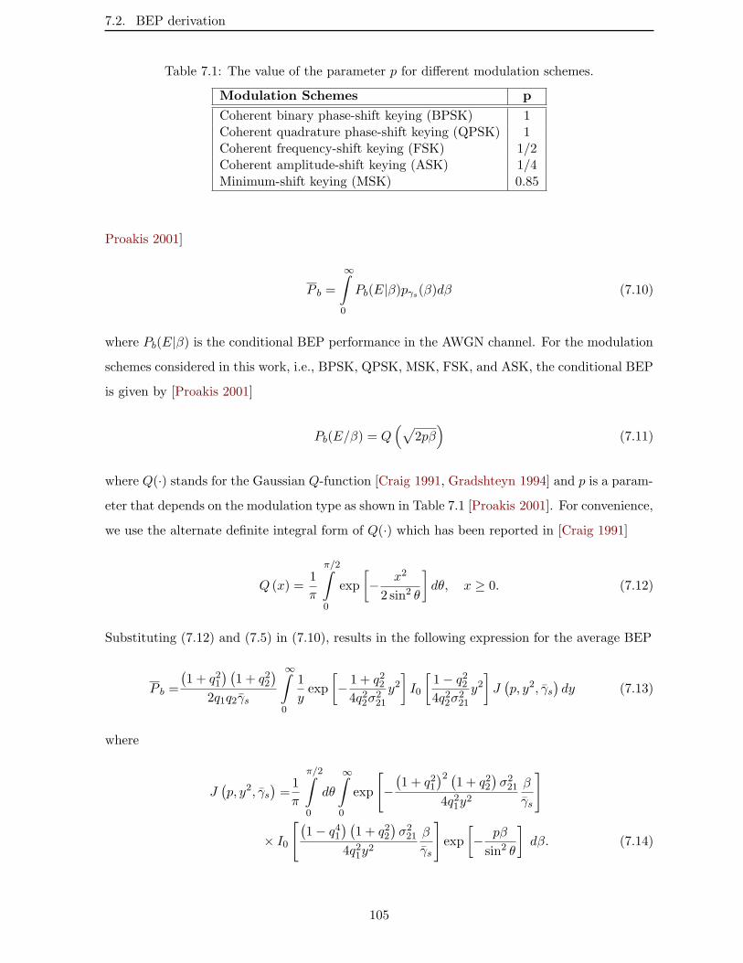
7.2. BEP derivation
Table 7.1: The value of the parameter p for different modulation schemes.
Modulation Schemes p
Coherent binary phase-shift keying (BPSK) 1Coherent quadrature phase-shift keying (QPSK) 1Coherent frequency-shift keying (FSK) 1/2Coherent amplitude-shift keying (ASK) 1/4Minimum-shift keying (MSK) 0.85
Proakis 2001]
P b =
∞∫
0
Pb(E|β)pγs(β)dβ (7.10)
where Pb(E|β) is the conditional BEP performance in the AWGN channel. For the modulation
schemes considered in this work, i.e., BPSK, QPSK, MSK, FSK, and ASK, the conditional BEP
is given by [Proakis 2001]
Pb(E/β) = Q(√
2pβ)
(7.11)
where Q(·) stands for the Gaussian Q-function [Craig 1991, Gradshteyn 1994] and p is a param-
eter that depends on the modulation type as shown in Table 7.1 [Proakis 2001]. For convenience,
we use the alternate definite integral form of Q(·) which has been reported in [Craig 1991]
Q (x) =1
π
π/2∫
0
exp
[− x2
2 sin2 θ
]dθ, x ≥ 0. (7.12)
Substituting (7.12) and (7.5) in (7.10), results in the following expression for the average BEP
P b =
(1 + q21
) (1 + q22
)
2q1q2γs
∞∫
0
1
yexp
[− 1 + q224q22σ
221
y2]I0
[1− q224q22σ
221
y2]J(p, y2, γs
)dy (7.13)
where
J(p, y2, γs
)=1
π
π/2∫
0
dθ
∞∫
0
exp
[−(1 + q21
)2 (1 + q22
)σ221
4q21y2
β
γs
]
× I0
[(1− q41
) (1 + q22
)σ221
4q21y2
β
γs
]exp
[− pβ
sin2 θ
]dβ. (7.14)
105
7.2. BEP derivation
Now, using [Gradshteyn 1994, Eq. 6.611(4.8)], the semi-infinite range integration in (7.14) can
be carried out. This leads to
J(p, y2, γs
)=
1
π
π/2∫
0
sin2 θ√(p+
(1+q21)(1+q22)σ2
12
2q21y2γs
sin2 θ
)(p+
(1+q21)(1+q22)σ2
12
2y2γssin2 θ
)dθ (7.15)
Finally, resubstituting (7.15) in (7.13), yields the following solution for the average BEP per-
formance
P b =
(1 + q21
) (1 + q22
)
2πq1q2γs
∞∫
0
π/2∫
0
1
yexp
[− 1 + q224q22σ
221
y2]I0
[1− q224q22σ
221
y2]
× sin2 θ√(p+
(1+q21)(1+q22)σ2
12
2q21y2γs
sin2 θ
)(p+
(1+q21)(1+q22)σ2
12
2y2γssin2 θ
) dθdy. (7.16)
The integrals involved in (7.16) are then computed numerically. In the following, we examine
the special cases of the obtained average BEP. For the double Rayleigh fading channel, i.e.,
q1 = q2 = 1, (7.16) can be simplified. Specifically, using [Gradshteyn 1994, Eq. 6.631(3)] and
doing some algebraic manipulations, the average BEP P b is reduced to the following exact result
P b =1
π√gγs
π/2∫
0
sin θ exp
[sin2 θ
2pγs
]W−1/2,0
(sin2 θ
pγs
)dθ (7.17)
whereW−1/2,0 (·) represents the Whittaker function defined by [Gradshteyn 1994, Eq. 9.222(2)].
Similarly, for the special case of the double one-sided Gaussian model, i.e., q1 → 0 and q2 → 0,
based on the use of [Gradshteyn 1994][Eqs. 6.618 (3), 1.411 (9), and (9.72)], (7.16) becomes
P b =1
2π3/2√gγs
π/2∫
0
sin θ exp
[sin2 θ
8pγs
]K0
(sin2 θ
8pγs
)dθ. (7.18)
Again, for q1 = 1 and q2 → 0, i.e., the case of the Rayleigh×one-sided Gaussian fading channel,
the BEP expression can be simplified by using [Gradshteyn 1994, Eq. 3.322 (2)]. This leads to
the result given by
P b =1√
2πgγs
π/2∫
0
sin θ exp
[sin2 θ
2pγs
]erfc
(sin θ√2pγs
)dθ (7.19)
106
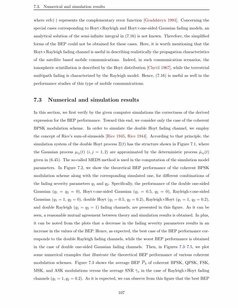
7.3. Numerical and simulation results
where erfc(·) represents the complementary error function [Gradshteyn 1994]. Concerning the
special cases corresponding to Hoyt×Rayleigh and Hoyt×one-sided Gaussian fading models, an
analytical solution of the semi-infinite integral in (7.16) is not known. Therefore, the simplified
forms of the BEP could not be obtained for these cases. Here, it is worth mentioning that the
Hoyt×Rayleigh fading channel is useful in describing realistically the propagation characteristics
of the satellite based mobile communications. Indeed, in such communication scenarios, the
ionospheric scintillation is described by the Hoyt distribution [Chytil 1967], while the terrestrial
multipath fading is characterized by the Rayleigh model. Hence, (7.16) is useful as well in the
performance studies of this type of mobile communications.
7.3 Numerical and simulation results
In this section, we first verify by the given computer simulations the correctness of the derived
expression for the BEP performance. Toward this end, we consider only the case of the coherent
BPSK modulation scheme. In order to simulate the double Hoyt fading channel, we employ
the concept of Rice’s sum-of-sinusoids [Rice 1945, Rice 1944]. According to that principle, the
simulation system of the double Hoyt process Ξ(t) has the structure shown in Figure 7.1, where
the Gaussian process µij(t) (i, j = 1, 2) are approximated by the deterministic process µij(t)
given in (6.45). The so-called MEDS method is used in the computation of the simulation model
parameters. In Figure 7.2, we show the theoretical BEP performance of the coherent BPSK
modulation scheme along with the corresponding simulated one, for different combinations of
the fading severity parameters q1 and q2. Specifically, the performance of the double one-sided
Gaussian (q1 = q2 = 0), Hoyt×one-sided Gaussian (q1 = 0.5, q2 = 0), Rayleigh×one-sided
Gaussian (q1 = 1, q2 = 0), double Hoyt (q1 = 0.5, q2 = 0.2), Rayleigh×Hoyt (q1 = 1, q2 = 0.2),
and double Rayleigh (q1 = q2 = 1) fading channels, are presented in this figure. As it can be
seen, a reasonable mutual agreement between theory and simulation results is obtained. In plus,
it can be noted from the plots that a decrease in the fading severity parameters results in an
increase in the values of the BEP. Hence, as expected, the best case of the BEP performance cor-
responds to the double Rayleigh fading channels, while the worst BEP performance is obtained
in the case of double one-sided Gaussian fading channels. Then, in Figures 7.3–7.5, we plot
some numerical examples that illustrate the theoretical BEP performance of various coherent
modulation schemes. Figure 7.3 shows the average BEP P b of coherent BPSK, QPSK, FSK,
MSK, and ASK modulations versus the average SNR γs in the case of Rayleigh×Hoyt fading
channels (q1 = 1, q2 = 0.2). As it is expected, we can observe from this figure that the best BEP
107
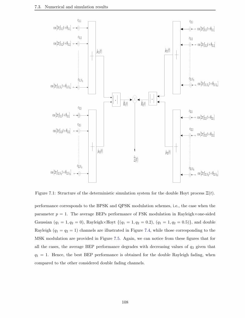
7.3. Numerical and simulation results
cos [2πf12,N12t + θ12,N12
]
µ11(t)
Ξ(t)
R1(t)
µ12(t)
µ21(t)
cos [2πf21,1t + θ21,1]
c21,1
c21,2
c21,N21
cos [2πf21,2t + θ21,2]
cos [2πf21,N21t + θ21,N21
]
R2(t)
µ22(t)
. .c22,1
c22,2
c22,N22
cos [2πf22,1t + θ22,1]
cos [2πf22,2t + θ22,2]
cos [2πf22,N22t + θ22,N22
]
c12,N12
c12,1
c12,1
c11,N11
c11,2
c11,1
cos [2πf11,N11t + θ11,N11
]
cos [2πf11,2t + θ11,2]
cos [2πf11,1t + θ11,1]
cos [2πf12,1t + θ12,1]
cos [2πf12,2t + θ12,2]
Figure 7.1: Structure of the deterministic simulation system for the double Hoyt process Ξ(t).
performance corresponds to the BPSK and QPSK modulation schemes, i.e., the case when the
parameter p = 1. The average BEPs performance of FSK modulation in Rayleigh×one-sided
Gaussian (q1 = 1, q2 = 0), Rayleigh×Hoyt (q1 = 1, q2 = 0.2), (q1 = 1, q2 = 0.5), and double
Rayleigh (q1 = q2 = 1) channels are illustrated in Figure 7.4, while those corresponding to the
MSK modulation are provided in Figure 7.5. Again, we can notice from these figures that for
all the cases, the average BEP performance degrades with decreasing values of q2 given that
q1 = 1. Hence, the best BEP performance is obtained for the double Rayleigh fading, when
compared to the other considered double fading channels.
108
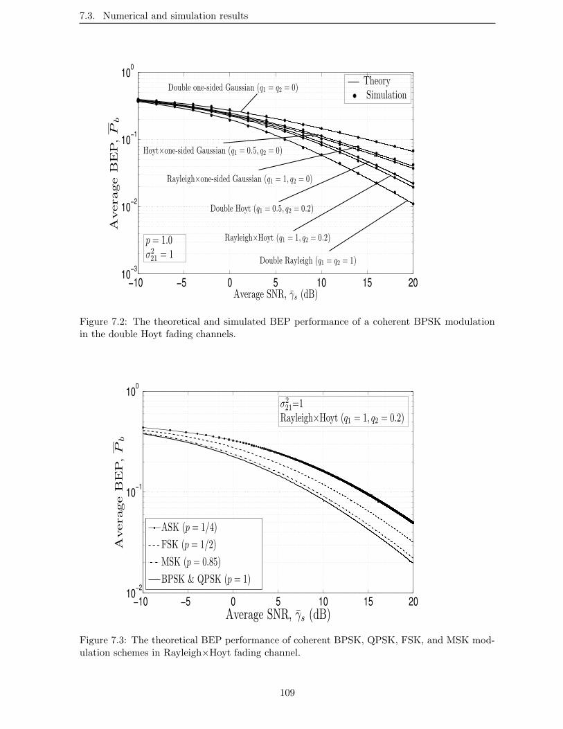
7.3. Numerical and simulation results
−10 −5 0 5 10 15 2010−3
10−2
10−1
100
Average SNR, γs (dB)
Average
BE
P,Pb
TheorySimulation
Rayleigh×Hoyt (q1 = 1, q2 = 0.2)
Rayleigh×one-sided Gaussian (q1 = 1, q2 = 0)
Double Hoyt (q1 = 0.5, q2 = 0.2)
Double Rayleigh (q1 = q2 = 1)
p = 1.0σ2
21 = 1
Double one-sided Gaussian (q1 = q2 = 0)
Hoyt×one-sided Gaussian (q1 = 0.5, q2 = 0)
Figure 7.2: The theoretical and simulated BEP performance of a coherent BPSK modulationin the double Hoyt fading channels.
−10 −5 0 5 10 15 2010−2
10−1
100
Average SNR, γs (dB)
Average
BE
P,Pb
ASK (p = 1/4)
FSK (p = 1/2)
MSK (p = 0.85)
BPSK & QPSK (p = 1)
σ221=1
Rayleigh×Hoyt (q1 = 1, q2 = 0.2)
Figure 7.3: The theoretical BEP performance of coherent BPSK, QPSK, FSK, and MSK mod-ulation schemes in Rayleigh×Hoyt fading channel.
109
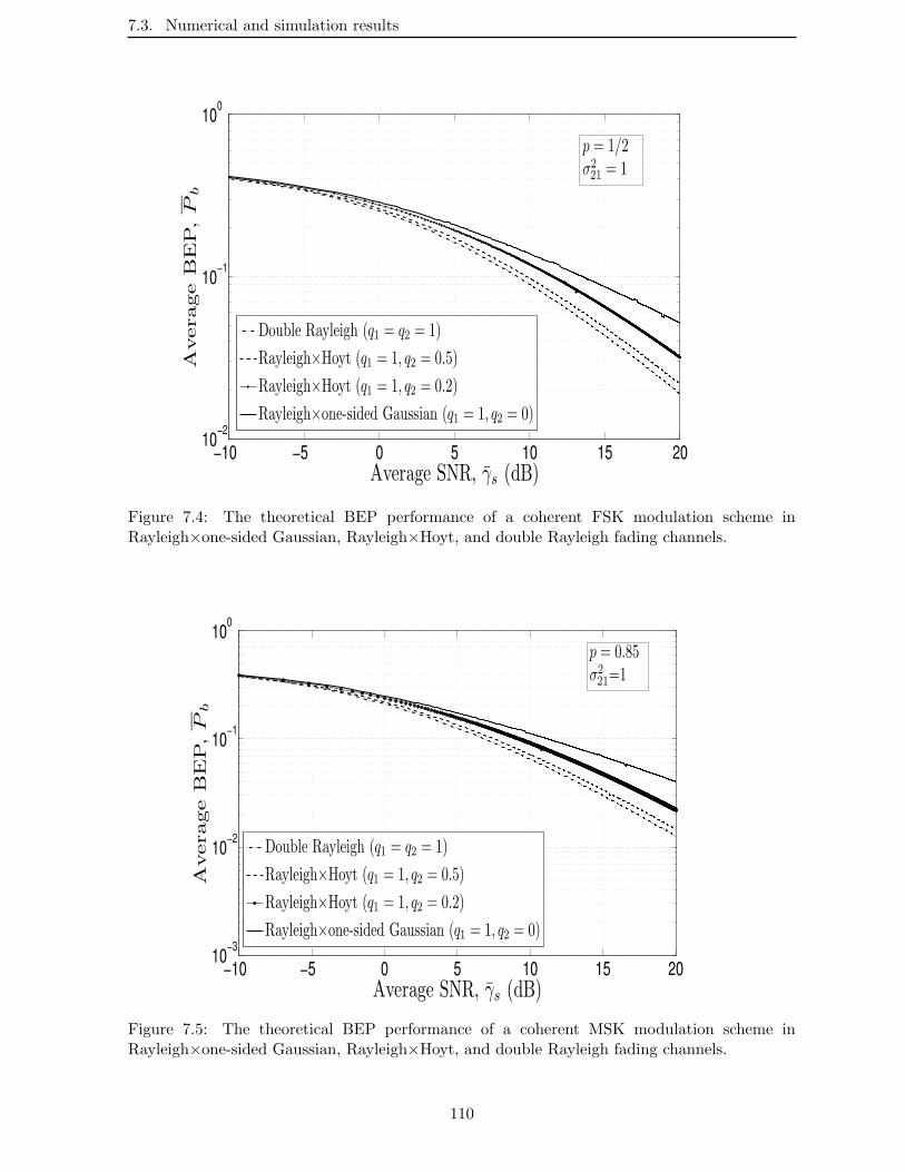
7.3. Numerical and simulation results
−10 −5 0 5 10 15 2010−2
10−1
100
Average SNR, γs (dB)
Average
BE
P,Pb
Double Rayleigh (q1 = q2 = 1)
Rayleigh×Hoyt (q1 = 1, q2 = 0.5)
Rayleigh×Hoyt (q1 = 1, q2 = 0.2)
Rayleigh×one-sided Gaussian (q1 = 1, q2 = 0)
p = 1/2σ2
21 = 1
Figure 7.4: The theoretical BEP performance of a coherent FSK modulation scheme inRayleigh×one-sided Gaussian, Rayleigh×Hoyt, and double Rayleigh fading channels.
−10 −5 0 5 10 15 2010−3
10−2
10−1
100
Average SNR, γs (dB)
Average
BE
P,Pb
Double Rayleigh (q1 = q2 = 1)
Rayleigh×Hoyt (q1 = 1, q2 = 0.5)
Rayleigh×Hoyt (q1 = 1, q2 = 0.2)
Rayleigh×one-sided Gaussian (q1 = 1, q2 = 0)
p = 0.85σ2
21=1
Figure 7.5: The theoretical BEP performance of a coherent MSK modulation scheme inRayleigh×one-sided Gaussian, Rayleigh×Hoyt, and double Rayleigh fading channels.
110
7.4. Conclusion
7.4 Conclusion
In this chapter, we studied the BEP performance of the digital modulated signals that are
transmitted over slow and frequency-flat double Hoyt fading channels. Specifically, an expression
for the average BEP of coherent BPSK, QPSK, FSK, MSK, and ASK modulation schemes has
been derived. The obtained BEP result is general and includes several special cases of the
double Hoyt fading channel. Furthermore, the validity of the theoretical expression has been
confirmed by computer simulations for the case of BPSK. The results presented in this chapter
are useful in the performance assessment of the M2M communication systems operating over
propagation environments characterized by fading conditions that are more severe than the
double Rayleigh fading. They can also be applied in mobile satellite communications when
the overall propagation channel can be statistically described by the Hoyt×Rayleigh fading
distribution.
111
Chapter 8
Conclusions and outlook
The performance analysis of wireless communications, taking into account the appropriate prop-
agation characteristics, is essential and highly relevant for designing and optimizing wireless
systems. Indeed, this analysis is generally used for verifying whether or not the system under
design is capable to meet the specific propagation conditions. Motivated by this fact and given
the importance of the M2M communications, which are becoming more and more useful in
future wireless systems, the main purpose of this thesis is to provide a performance analysis on
wireless M2M communications over the Hoyt fading channels. As is known, the Hoyt fading
model is a general multipath fading distribution, which includes the one-sided and Rayleigh
fading models as special cases. It also has the advantage of approximating the Nakagami-m
distribution in the range of the fading severity between 0.5 and 1 and vice versa.
Specifically, the objective of this thesis has to contribute to the topic of performance analysis
of various digital modulation schemes commonly used in wireless communication systems over
the M2M Hoyt fading channels. In this context, this thesis work has been divided into two
essential parts. Regarding the first part, which has been exposed in chapters 3, 4, and 5, we
have focussed on the topic of the performance analysis of various digital modulation schemes,
especially DPSK and FSK with LDI and differential detections, over the M2M single Hoyt fading
channels. In this context, significant findings have been obtained. Namely, a formula for the
average number of FM clicks occurring at the output of a discriminator FM receiver has been
derived. In addition, a closed-form expression for the PDF of the phase difference between two
phases or frequency modulated signals transmitted over the Hoyt fading channels and perturbed
by the correlated Gaussian noise has been presented. All the above derived formulas have been
validated by reducing them to the Rayleigh fading channel as a special case of the Hoyt fading.
Furthermore, the presented PDF expression of the overall phase difference has also been checked
by comparing it with that obtained from computer simulations, considering a M2M single Hoyt
fading channel. Then, based upon this PDF, closed-form expressions for the BEP performance
of the above mentioned modulation schemes that are transmitted over the M2M single Hoyt
fading channels have been derived and verified to include the special case corresponding to
the Rayleigh fading channel. From the obtained BEP results, it has been concluded that the
112
8. Conclusions and outlook
BEP performance degrades with decreasing values of the Hoyt fading severity parameter q and,
therefore, the lowest BEP has been obtained for the Rayleigh fading channel, i.e., q = 1, while
the highest one corresponds to the one-sided Gaussian channel, i.e., q = 0.
Then, in the second part of this thesis, where the corresponding main findings have been
presented in chapters 6 and 7, we have introduced the cascaded or double Hoyt fading channels.
These scattering fading channels, where the overall complex channel gain between the transmit-
ter and receiver is modeled as the product of the gains of two statistically independent single
Hoyt fading channels, can be used in the channel modeling of more realistic and appropriate
M2M communication systems operating over propagation environments characterized by fading
conditions that are more severe than those described by the double Rayleigh fading. Consid-
ering this double scattering channel model, a study on its main statistical properties has been
investigated. Namely, analytical expressions for the performance measures commonly used in
wireless communications especially, the CDF, LCR, and ADF which are useful for studying the
outage probability, frequency of outages, and average outage duration, respectively, have been
derived. Furthermore, the first and second order statistics of the capacity of the double Hoyt
fading channels have also been studied. In addition to all these investigated performance mea-
sures, we have studied in this part, hereafter, the impact of slowly varying frequency flat double
Hoyt propagation environments on the error rate performance of coherent BPSK, QPSK, FSK,
MSK, and ASK modulation schemes. Hence, a closed-form expression for the average BEP of
all these coherent modulation schemes has been investigated. The obtained BEP expression is
general and includes, as special cases, results corresponding to the channel combinations given
by Rayleigh×Hoyt, Rayleigh×one-sided Gaussian, Hoyt×one-sided Gaussian, double one-sided
Gaussian, and double Rayleigh fading channels. Furthermore, the validity of the obtained the-
oretical results has been checked by means of computer simulations for some of the modulation
schemes used in the analysis. It has also been concluded from the presented BEP results, for
all considered modulation schemes, that a decrease in the fading severity parameters q1 and q2,
which characterize the double Hoyt fading channels, results in an increase in the values of the
BEP. Hence, the best case of the BEP performance has corresponded to the double Rayleigh
fading channels, i.e., q1 = q2 = 1, while the worst one has been obtained in the case of double
one-sided Gaussian fading channels, i.e., the case when q1 = q2 = 0.
Let us now close this dissertation with the following key ideas for possible future research.
A significant enhancement, in this work, would be the extension of the presented performance
analysis studies on SISO M2M communications over the Hoyt fading channels to the case of
113
8. Conclusions and outlook
MIMO M2M Hoyt fading channels. As it is known, the employment of multiple antennas
at both the transmitter and receiver, i.e., MIMO technologies, is very promising for M2M
communications since it can be useful in combating the effects of fading and enables to greatly
improve the link reliability and increase the overall system capacity.
Another extension of this work can be done on the second part of the thesis, which deals with
the performance analysis of wireless M2M communications over the double Hoyt fading channels.
Indeed and in the presented analysis, we have assumed that the channel fading model is slow
and non-selective. This assumption would be extended by considering fast varying frequency-
selective double Hoyt fading channels, which reflect more realistic propagation environments
and high bandwidth transmissions, and try, thereafter, to evaluate the error rate performance
of the M2M communications over such fading channels.
Furthermore, the proposed double Hoyt fading model is restricted to a two-single hop . This
model can be extended and generalized by the Multihop cascaded Hoyt fading channels, i.e.,
N*Hoyt. Hence, a study on the statistical characterization of N*Hoyt fading channels as well as
their applications to a related performance analysis of wireless radio links can be investigated.
114

Appendix A
The BEP parameters for different
bit patterns due to ISI effects
This part complements chapter 3. Specifically, the various parameters needed in the calculation
of the BEP performance given by (3.39) for the three bit patterns “111”, “010”, and “011” are
presented.
• For “111” bit pattern
∆φ =πh
C1 = |H(h/2T )|2 , C2 = 0
N =2πd · h√[(|H(h/2T )|2 + e
)2− l2
] . (A-1)
• For “010” bit pattern
∆φ =2 tan−1 n11− n2
C1 =
[sin πh
2πh2
]2 [(1− n2)
2 + n21
], C2 = 0
φ(t) =π
T
[(n2 cos
2πtT − 1
)n1 sin
πtT − 2n1n2 cos
πtT sin 2πt
T(1− n2 cos
2πtT
)2+ n21 cos
2 πtT
]
a2(t) =
[sin πh
2πh2
]2·[(
1− n2 cos2πt
T
)2
+ n21 cos2 πt
T
]. (A-2)
where the quantities n1 and n2 are given by
n1 =2 |H(1/2T )| h2
1− h2cot(πh/2)
n2 =2 |H(1/T )| h2
4− h2(A-3)
115
BEP parameters for different bit patterns due to ISI
• For “011” bit pattern
∆φ =1
2[∆φ|111 + ∆φ|010]
N =1
2
[N∣∣111
+ N∣∣010
]. (A-4)
116
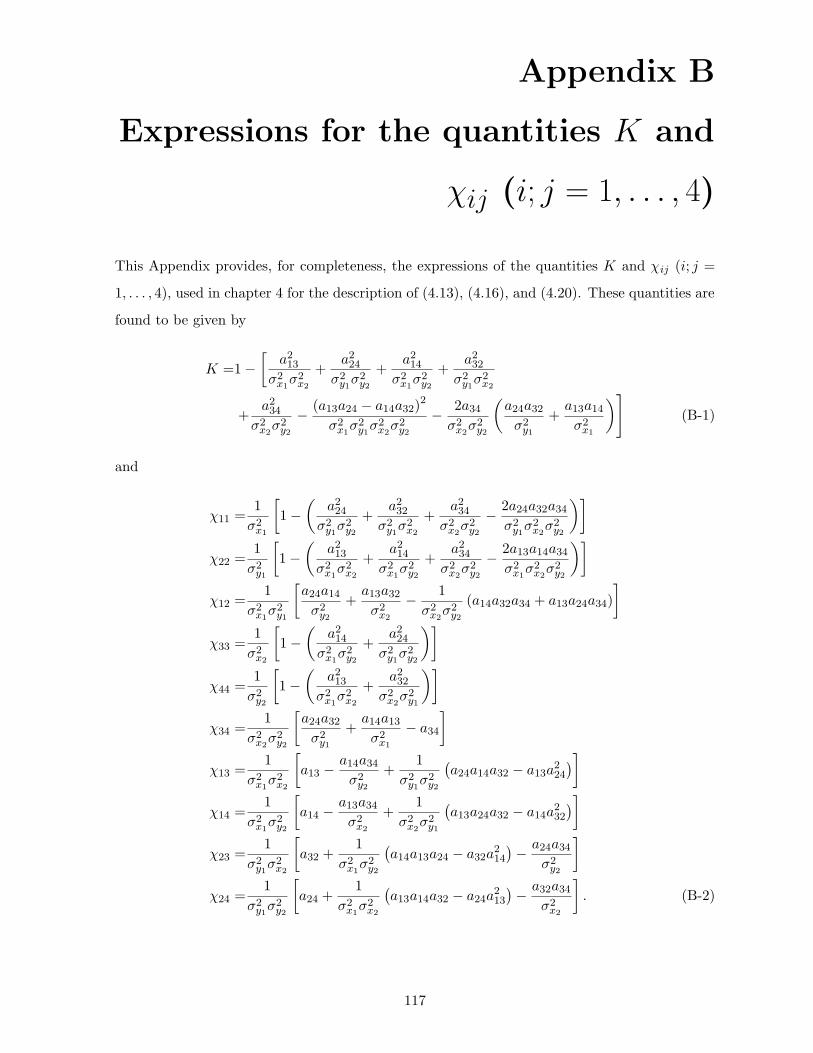
Appendix B
Expressions for the quantities K and
χij (i; j = 1, . . . , 4)
This Appendix provides, for completeness, the expressions of the quantities K and χij (i; j =
1, . . . , 4), used in chapter 4 for the description of (4.13), (4.16), and (4.20). These quantities are
found to be given by
K =1−[
a213σ2x1σ
2x2
+a224
σ2y1σ2y2
+a214
σ2x1σ2y2
+a232
σ2y1σ2x2
+a234
σ2x2σ2y2
− (a13a24 − a14a32)2
σ2x1σ2y1σ
2x2σ
2y2
− 2a34σ2x2σ
2y2
(a24a32σ2y1
+a13a14σ2x1
)](B-1)
and
χ11 =1
σ2x1
[1−
(a224
σ2y1σ2y2
+a232
σ2y1σ2x2
+a234
σ2x2σ2y2
− 2a24a32a34σ2y1σ
2x2σ
2y2
)]
χ22 =1
σ2y1
[1−
(a213
σ2x1σ2x2
+a214
σ2x1σ2y2
+a234
σ2x2σ2y2
− 2a13a14a34σ2x1σ
2x2σ
2y2
)]
χ12 =1
σ2x1σ2y1
[a24a14σ2y2
+a13a32σ2x2
− 1
σ2x2σ2y2
(a14a32a34 + a13a24a34)
]
χ33 =1
σ2x2
[1−
(a214
σ2x1σ2y2
+a224
σ2y1σ2y2
)]
χ44 =1
σ2y2
[1−
(a213
σ2x1σ2x2
+a232
σ2x2σ2y1
)]
χ34 =1
σ2x2σ2y2
[a24a32σ2y1
+a14a13σ2x1
− a34
]
χ13 =1
σ2x1σ2x2
[a13 −
a14a34σ2y2
+1
σ2y1σ2y2
(a24a14a32 − a13a
224
)]
χ14 =1
σ2x1σ2y2
[a14 −
a13a34σ2x2
+1
σ2x2σ2y1
(a13a24a32 − a14a
232
)]
χ23 =1
σ2y1σ2x2
[a32 +
1
σ2x1σ2y2
(a14a13a24 − a32a
214
)− a24a34
σ2y2
]
χ24 =1
σ2y1σ2y2
[a24 +
1
σ2x1σ2x2
(a13a14a32 − a24a
213
)− a32a34
σ2x2
]. (B-2)
117
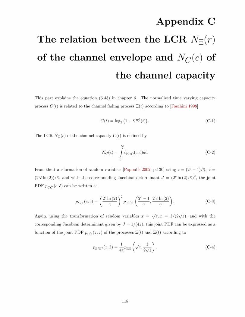
Appendix C
The relation between the LCR NΞ(r)
of the channel envelope and NC(c) of
the channel capacity
This part explains the equation (6.43) in chapter 6. The normalized time varying capacity
process C(t) is related to the channel fading process Ξ(t) according to [Foschini 1998]
C(t) = log2(1 + γ Ξ2(t)
). (C-1)
The LCR NC(c) of the channel capacity C(t) is defined by
NC(c) =
∞∫
0
cpCC(c, c)dc. (C-2)
From the transformation of random variables [Papoulis 2002, p.130] using z = (2c − 1)/γ, z =
(2cc ln (2))/γ, and with the corresponding Jacobian determinant J = (2c ln (2)/γ)2, the joint
PDF pCC (c, c) can be written as
pCC (c, c) =
(2c ln (2)
γ
)2
pΞ2Ξ2
(2c − 1
γ,2cc ln (2)
γ
). (C-3)
Again, using the transformation of random variables x =√z, x = z/(2
√z), and with the
corresponding Jacobian determinant given by J = 1/(4z), this joint PDF can be expressed as a
function of the joint PDF pΞΞ (z, z) of the processes Ξ(t) and Ξ(t) according to
pΞ2Ξ2(z, z) =1
4zpΞΞ
(√z,
z
2√z
). (C-4)
118
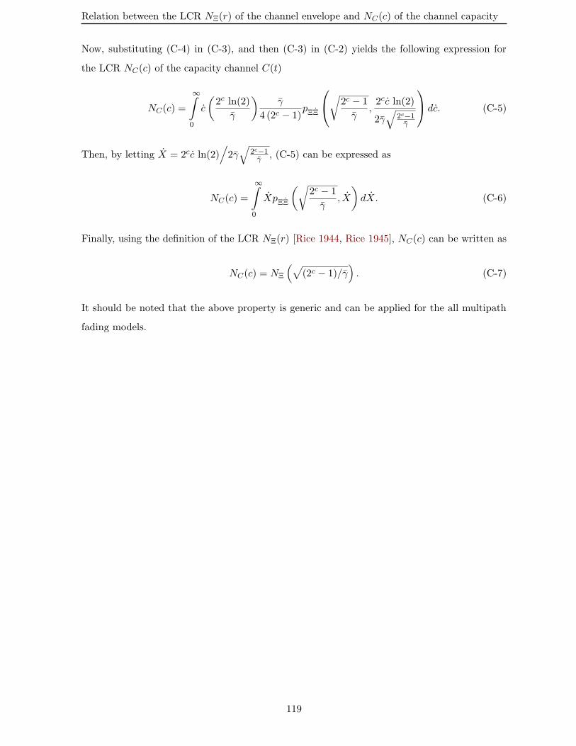
Relation between the LCR NΞ(r) of the channel envelope and NC(c) of the channel capacity
Now, substituting (C-4) in (C-3), and then (C-3) in (C-2) yields the following expression for
the LCR NC(c) of the capacity channel C(t)
NC(c) =
∞∫
0
c
(2c ln(2)
γ
)γ
4 (2c − 1)pΞΞ
√
2c − 1
γ,2cc ln(2)
2γ√
2c−1γ
dc. (C-5)
Then, by letting X = 2cc ln(2)/2γ√
2c−1γ , (C-5) can be expressed as
NC(c) =
∞∫
0
XpΞΞ
(√2c − 1
γ, X
)dX. (C-6)
Finally, using the definition of the LCR NΞ(r) [Rice 1944, Rice 1945], NC(c) can be written as
NC(c) = NΞ
(√(2c − 1)/γ
). (C-7)
It should be noted that the above property is generic and can be applied for the all multipath
fading models.
119
Bibliography
[Acosta 2004] G. Acosta, K. Tokuda and M. A. Ingram. Measured joint Doppler-delay power
profiles for vehicle-to-vehicle communications at 2.4 GHz. In IEEE Global Telecommu-
nications 2008(GLOBECOM’04), volume 6, pages 3813–3817, New Orleans-LA-USA,
Nov. 2004. 22, 23
[Adachi 1992] F. Adachi and T. T. Tjhung. Distribution of phase angle between two Rayleigh
vectors perturbed by Gaussian noise. IEEE Electronics Letters, vol. 28, no. 10, pages
923–925, May. 1992. 49, 56
[Adinoyi 2007] A. Adinoyi and H. Yanikomeroglu. Cooperative relaying in multi-antenna fixed
relay networks. IEEE Transactions on wireless communications, vol. 6, no. 1, pages 1–12,
Jan. 2007. 1
[Akki 1986] A. S. Akki and F. Haber. A Statistical model of mobile-to-mobile land communica-
tionchannel. IEEE Transactions on Vehicular Technology, vol. 35, pages 2–7, Feb. 1986.
1, 4, 22, 24, 25, 26, 27, 31, 57
[Akki 1994a] A. S. Akki. The influence of mobile-to-mobile land communication channel spec-
trum on the error rate of binary DPSK and NFSK matched filter receivers. IEEE Trans-
actions on Vehicular Technology, vol. 43, no. 4, pages 832–836, Mar. 1994. 2
[Akki 1994b] A. S. Akki. Statistical properties of mobile-to-mobile land communication chan-
nels. IEEE Transactions on Vehicular Technology, vol. 43, no. 4, pages 826–831, Nov.
1994. 22, 27, 29
[Ali 2007] O. B. S. Ali, B.L. Agba, C. Cardinal and F. Gagnon. Performance simulation of
flat fading channels in mobile ad hoc networks. In International Symposium on Signals,
Systems, and Electronics 2007 (ISSSE’07), pages 189–191, Monreal, Quebec, Aug. 2007.
2
[Almers 2006] P. Almers, F. Tufvesson and A. F. Molisch. Keyhole effect in MIMO wireless
channels: measurements and theory. IEEE Transactions on wireless communications,
vol. 5, no. 12, pages 976–978, Dec. 2006. 82
120
Bibliography
[Baid 2008] A. Baid, H. Fadnavis and P. R. Sahu. Performance of a predetection EGC receiver in
Hoyt fading channels for arbitrary number of branches. IEEE Communications Letters,
vol. 12, no. 9, pages 627–629, Sep. 2008. 11
[Bauge 2004] T. Bauge. Ad hoc networking in military scenarios. Thales Research and Tech-
nology (UK), no. 1, pages 1–5, May. 2004. http://www.thalesgroup.com. 21
[Boyer 2004] J. Boyer, D. D. Falconer and H. Yanikomeroglu. Multihop diversity in wireless
relaying channels. IEEE Transactions on Communications, vol. 52, no. 10, pages 1820–
1830, Oct. 2004. 22
[Bramley 1951] E. N. Bramley. Diversity effects in spaced-aerial reception of ionospheric waves.
In Proc. IEE, numero 1062R, pages 19–25, Jan. 1951. 56
[CCM 2007] Car2car communication consortium manifesto. Aug. 2007. http://www.
car-2-car.org/fileadmin/downloads/C2C-CC_manifesto_v1.1.pdf. 22
[Chai 1999] C. C. Chai. Distribution of phase difference between two Rice-or Nakagami-
Lognormal processes perturbed by Gaussian noise. In 50 th IEEE Vehicular Technology
Conference 1999 (VTC’99), volume 1, pages 82–86, 1999. 49
[Chelli 2007] A. Chelli and M. Patzold. A MIMO mobile-to-mobile channel model derived from
a geometric street scattering model. In 4th IEEE International Symposium on Wireless
Communication Systems (ISWCS’07), pages 792–797, Trondheim-Norway, Oct. 2007. 23
[Cheng 2008] X. Cheng, C.-X. Wang, D. I. Laurenson, H.-H. Chen and A. V. Vasilakos. A
generic geometrical-based MIMO mobile-to-mobile channel model. In International Wire-
less Communications and Mobile Computing Conference 2008(IWCMC’08), pages 1000–
1005, Crete Island-Greece, Aug. 2008. 23
[Chytil 1967] B. Chytil. The distribution of amplitude scintillation and the conversion of scintil-
lation indices. Journal of Atmospheric and Terrestrial Physics, vol. 29, pages 1175–1777,
Sep. 1967. 10, 102, 107
[Clarke 1968] R. H. Clarke. A statistical theory of mobile-radio reception. Bell System Technical
Journal, vol. 47, pages 957–1000, July/Aug. 1968. 17
[CouchII 2001] L. W. CouchII. Digital and analog communications systems. Prentice Hall, New
Jersey, 6th edition, 2001. 16
121
Bibliography
[Craig 1991] J. W. Craig. A new, simple, and exact result for calculating the probability of
error for two-dimentional signal constellations. In Proc IEEE Military Communications
Conference 1991, volume 2, pages 571–575, McLean, VA, USA, Nov. 1991. 105
[Crepeau 1992] P. J. Crepeau. Uncoded and coded performance of MFSK and DPSK in Nak-
agami fading channels. IEEE Transactions on Communications, vol. 40, no. 3, pages
487–493, Mar. 1992. 10
[Dohler 2003] M. Dohler. Virtual antenna arrays. Ph.D. dissertation, Kings College London,
London, United Kingdom, 2003. 22
[Duong 2007] T. Q. Duong, H. Shin and E-K. Hong. Error probability of binary and M -ary
signals with spatial diversity in Nakagamai-q(Hoyt) fading channels. EURASIP Journal
on Wireless Communications and Networking, vol. 2007, Oct. 2007. 12
[Ercerg 1997] V. Ercerg, S. J. Fortune, J. Ling and R. A. Valenzuela. Bilateral averaging
over receiving and transmitting areas for accurate measurements of sector average signal
strength inside buildings. IEEE Journal on Selected Areas in Communication, vol. 15,
no. 4, pages 677–684, May. 1997. 23
[Fedele 1995] G. Fedele, L. Izzo and M. Tanda. Distribution of phase difference between two
Nakagami faded signals perturbed by Gaussian noise. IEE Electronics Letters, vol. 31,
no. 7, pages 526–527, Mar. 1995. 49
[Foschini 1998] G. J. Foschini and M. J. Gans. On limits of wireless communications in a fading
environment when using multiple antennas. Wireless Personal Communications, vol. 6,
pages 311–335, 1998. 89, 118
[Fraidenraich 2005] G. Fraidenraich, J. C. S. S. Filho and M. D. Yacoub. Second-Order statis-
tics of maximal-ratio and equal-gain Combining in Hoyt fading. IEEE Communications
Letters, vol. 9, no. 1, pages 19–21, Jan. 2005. 11
[Gesbert 2002] D. Gesbert, H. Bolcskei, D. A. Gore and A. J. Paulraj. Outdoor MIMO wireless
channels: models and performance prediction. IEEE Transactions on communications,
vol. 50, no. 12, pages 1926–1934, Dec. 2002. 82
[Gradshteyn 1994] I. S. Gradshteyn and I. M. Ryzhik. Tables of integrals, series, and products.
New York: Academic, 5th edition, Jan. 1994. 11, 13, 17, 27, 31, 41, 42, 56, 84, 86, 88,
104, 105, 106, 107
122
Bibliography
[Guizani 2004] M. Guizani. Wireless communications systems and networks. Kluwer Academic
Publishers New York, 2004. 7
[Hadzi-Velkov 2008] Z. Hadzi-Velkov, N. Zlatanov and G. K. Karagiannidis. On the second
order statistics of the multihop Rayleigh fading channel. IEEE Transactions on commu-
nications, vol. 56, no. XX, pages 1–9, Month. 2008. 81
[Hagras 2001] E. A. Hagras, K. A. M. Soilman and F. A. Chadi. Performance analysis of
GMSK with CSDD and CSDDD scheme in land mobile-to-mobile channel with random
frequency shifts and CCI. In Eighteenth National Radio Science Conference, pages 1–9,
Mansoura, Egypt, Mar. 2001. 2
[Hajri 2005] N. Hajri, N. Youssef and M. Patzold. Simulation of mobile-to-mobile radio fading
channels. In 12th IEEE International Conference on Electronics, Circuits and Systems
2005(ICECS’05), pages 349–352, Gammarth-Tunisia, Dec. 2005. 24, 57, 58, 66, 93
[Honcharenko 1995] W. Honcharenko, H. L. Bertoni and J. L. Dailing. Bilateral averaging
over receiving and transmitting areas for accurate measurements of sector average signal
strength inside buildings. IEEE Transactions on Antennas and Propagation, vol. 43,
no. 5, pages 508–512, May. 1995. 23
[Hoyt 1947] R. S. Hoyt. Probability functions for the modulus and angle of the normal complex
variate. Bell System Technical Journal, vol. 26, pages 318–359, Apr. 1947. 2, 10, 12, 13,
14
[Iskander 2008] C. D. Iskander and P. T. Mathiopoulos. Exact performance analysis of dual-
branch equal-gain combining in Nakagami-m, Rician and Hoyt fading. IEEE Transac-
tions on Vehicular Technology, vol. 57, no. 2, pages 921–931, Mar. 2008. 11
[Jakes 1993] W. C. Jakes. Microwave mobile communications. NJ: IEEE Press, 2nd edition,
1993. 17, 18, 19, 20, 29, 36, 66, 68, 89, 95
[Karagiannidis 2005] G. K. Karagiannidis, N. C. Sagias and D. A. Zogas. Error analysis of M -
QAM with equal-gain diversity over generalized fading channels. IEE Proc. Commun,
vol. 152, no. 1, pages 69–74, Feb. 2005. 11
[Karagiannidis 2007] G. K. Karagiannidis, N. C. Sagias and P. T. Mathiopoulos. N∗Nakagami:
a novel stochastic model for cascaded fading channels. IEEE Transactions on communi-
cations, vol. 55, no. 8, pages 1453–1458, Aug. 2007. 81
123
Bibliography
[Korn 1990a] I. Korn. M -ary FSK with limiter discriminator integrator detection and DPSK
with differentiel phase detection in Rician fading channel. International Journal on
Satellite Communcations, vol. 8, pages 363–368, 1990. 34
[Korn 1990b] I. Korn. M -ary frequency shift keying with limiter-discriminator integrator detec-
tor in satellite mobile channel with narrow-band receiver filter. IEEE Transactions on
wireless communications, vol. 38, no. 10, pages 1771–1778, Oct. 1990. 34
[Korn 2001] I. Korn and J. P. Fonseka. M -CPM with MRC diversity in Rician-, Hoyt-, and
Nakagami-fading channels. IEEE Transactions on Vehicular Technology, vol. 50, no. 4,
pages 1182–1189, Jul. 2001. 11
[Kovacs 2002a] I. Z. Kovacs. Radio channel characterization for private mobile radio systems.
Ph.D. dissertation, Aalborg University, Center for PersonKommunikation, 2002. 1, 22,
23, 30, 31, 81, 85, 86, 87
[Kovacs 2002b] I. Z. Kovacs, P. C. F. Eggers, K. Olesen and L. G. Petersen. Investigations
of outdoor-to-indoor mobile-to-mobile radio communications channels. In IEEE 56th
Vehicular Technology Conference 2002 (VTC’02), volume 1, pages 430–434, Vancouver-
Canada, Sep. 2002. 1, 22, 24, 30, 31
[Laneman 2001] J. N. Laneman, G. W. Wornell and D. N. C. Tse. An efficient protocol for
realizing cooperative diversity in wireless networks. In IEEE Internationl Symposium on
Information Theory Conference 2001 (ISIT’01), page 294, Washington-DC, Jun. 2001.
22, 32
[Laneman 2004] J. N. Laneman, D. N. C. Tse and G. W. Wornell. Cooperative diversity in wire-
less networks: effcient protocols and outage behavior. IEEE Transactions on Information
Theory, vol. 50, no. 12, pages 3062–3080, Dec. 2004. 22, 32
[Lee 1975] J. S. Lee and L. E. Miller. On the binary DPSK communication systems in correlated
Gaussian noise. IEEE Transactions on communications, vol. 23, no. 2, pages 255–259,
Feb. 1975. 64, 65
[Linnartz 1996] J-P. M. Linnartz and R. F. Diesta. Research Reports: Evaluation Of Radio
Links And Networks. Institute of Transportation Studies California Partners for Ad-
vanced Transit and Highways (PATH), Jun. 1996. http://repositories.cdlib.org/
its/path/reports/UCB-ITS-PRR-96-16. 22, 23
124
Bibliography
[Liu 2006] X. Liu and L. Hanzo. Exact BER calculation of asynchronous DS-CDMA systems
communicating over Hoyt channels. In 9th IEEE International Symposium on Spread
Spectrum Techniques and Applications 2006(ISSSTA’06), pages 337–341, Manaus, Ama-
zon, Brazil, Aug. 2006. 11
[Ma 2007] Y. Ma and M. Patzold. Wideband two-ring MIMO channel models for mobile-to-
mobile communications. In 10th International Symposium on Wireless Personal Multi-
media Communications (WPMC’07), pages 380–384, Jaipur India, Oct. 2007. 23
[Mason 1987] L. J. Mason. An error probability formula for M -ary DPSK in fast Rician fading
and Gaussian noise. IEEE Transactions on communications, vol. COM-35, no. 9, pages
976–978, 1987. 49
[Maurer 2002] J. Maurer, T. Fugen and W. Wiesbeck. Narrow-band measurement and analysis
of the inter-vehicle transmission channel at 5.2 GHz. In IEEE 55th Vehicular Technology
Conference 2002 (VTC’02), volume 3, pages 1274–1278, Birmingham-Al, May. 2002. 22,
23
[Miyagaki 1979] Y. Miyagaki, N. Morinaga and T. Namekawa. Error probability considerations
for M -ary DPSK signal in land mobile radio. Trans. Inst. Electron. Commun. Eng.
Japan, vol. 62-B, no. 6, pages 581–588, Jun. 1979. 62
[Nakagami 1960] M. Nakagami. The m-distribution—A general formula of intensity distribution
of fading. In Statistical Methods in Radio Wave Propagation, pages 3–36. New York:
Pergamon, 1960. 2, 10, 13, 14, 82
[Ng 1994] C. S. Ng, T. T. Tjhung, F. Adachi and F. P. S. Chin. Closed-form error probability for-
mula for narrow-band FSK, with limiter-discriminator-integrator detection, in Rayleigh
fading. IEEE Transactions on communications, vol. 42, no. 10, pages 2795–2802, Oct.
1994. 34, 70, 71, 75
[Pabst 2004] R. Pabst, B. H. Walke, D. C. Schultz, P. Herhold, H. Yanikomeroglu, S. Mukherjee,
H. Viswanathan, M. Lott, W. Zirwas, M. Dohler, H. Aghvami, D. D. Falconer and G. P.
Fettweis. Relay-based deployment concepts for wireless and mobile broadband radio. IEEE
Communications Magazine, vol. 42, pages 80–89, Sep. 2004. 22
[Papoulis 2002] A. Papoulis and S. U. Pillai. Probability, random variables and stochastic
processes. New York: McGraw-Hill, 4th edition, 2002. 16, 25, 84, 85, 86, 90, 103, 118
125
Bibliography
[PAT 2008] Path Research Program, 2008. http://www.path.berkeley.edu. 22
[Patel 2003] C. S. Patel, G.L. Stuber and T. G. Pratt. Simulation of Rayleigh-faded mobile-to-
mobile communication channels. In IEEE 58th Vehicular Technology Conference 2003
(VTC’03), volume 1, pages 163–167, Orlando-Florida-USA, Oct. 2003. 23
[Patel 2005] C. S. Patel, G.L. Stuber and T. G. Pratt. Simulation of Rayleigh-faded mobile-to-
mobile communication channels. IEEE Transactions on communications, vol. 53, no. 11,
pages 1876–1884, Nov. 2005. 23, 24, 29, 30
[Patel 2006] C. S. Patel, G.L. Stuber and T. G. Pratt. Statistical properties of amplify and
forward relay fading channels. IEEE Transactions on Vehicular Technology, vol. 55,
no. 1, pages 1–9, Jan. 2006. 22, 32, 33, 81, 88
[Patzold 2002] M. Patzold. Mobile fading channels. John Wiley & Sons, LTD, 2002. 17, 24,
58, 66, 87, 93
[Patzold 2005a] M. Patzold, B. 0. Hogstad, N. Youssef and D. Kim. A MIMO mobile-to-mobile
channel model: Part I — The reference model. In 16th IEEE International Symposium
on Personnal, Indoor and Mobile Radio Communication (PIMRC’05), pages 573–578,
Berlin-Germany, Sept. 2005. 23
[Patzold 2005b] M. Patzold, B. 0. Hogstad, N. Youssef and D. Kim. A MIMO mobile-to-mobile
channel model: Part II — The simulation model. In 16th IEEE International Symposium
on Personnal, Indoor and Mobile Radio Communication (PIMRC’05), pages 562–567,
Sept. 2005. 24
[Patzold 2008] M. Patzold, B. O. Hogstad and N. Youssef. Modeling, analysis, and simulation
of MIMO mobile-to-mobile fading channels. IEEE Transactions on wireless communica-
tions, vol. 7, no. 2, pages 510–520, Feb. 2008. 23, 24
[Pawula 1981] R. F. Pawula. On the theory of error rates for narrow-band digital FM. IEEE
Transactions on communications, vol. COM-29, pages 1634–1643, Nov. 1981. 36, 37, 41,
43, 44, 49, 71, 75
[Pawula 1982] R. F. Pawula, S. O. Rice and J. H. Roberts. Distribution of the phase angle
between two vectors perturbed by Gaussian noise. IEEE Transactions on communications,
vol. COM-30, no. 8, pages 1828–1841, Aug. 1982. 49
126
Bibliography
[Pawula 1984] R. F. Pawula. Offset DPSK and a comparison of conventional and symmetric
DPSK with noise correlation and power imbalance. IEEE Transactions on communica-
tions, vol. COM-32, no. 3, pages 233–240, Mar. 1984. 64, 65
[Peden 2004] M. Peden, R. Scurfield, D. Sleet, D. Mohan, A. A. Hyder, E. Jarawan and C. Math-
ers. World report on road traffic injury prevention. World Health Organization Geneva
press, 2004. http://whqlibdoc.who.int/publications/2004/9241562609.pdf. 22
[Plesse 2004] T. Plesse, C. Adjih, P. Minet, A. Laouiti, A. Plakoo, M. Badel, P. Muhlethaler,
P. Jacquet and J. Lecomte. OLSR performance measurement in a military mobile ad-hoc
network. In 24th International Conference on Distributed Computing Systems Work-
shops 2004 (ICDCSW04), pages 704–709, Tokyo-Japan, Mar. 2004. 21
[Proakis 2001] J. G. Proakis. Digital communications. New York: McGraw-Hill, 4th edition edi-
tion, 2001. 63, 102, 105
[Radaydeh 2007] R. M. Radaydeh. Average error performance of M -ary modulation schemes
in Nakagamai-q(Hoyt) fading channels. IEEE Communications Letters, vol. 11, no. 3,
pages 255–257, Mar. 2007. 12
[Radaydeh 2008a] R. M. Radaydeh and M. M. Matalgah. Non-coherent improved-gain diver-
sity reception of binary orthogonal signals in Nakagami-q (Hoyt) mobile channels. IET
Commun, vol. 2, no. 2, pages 372–379, Feb. 2008. 12
[Radaydeh 2008b] R. M. Radaydeh and M. M. Matalgah. Compact formulas for the aver-
age error performance of noncoherent M -ary orthogonal signals over generalized Rician,
Nakagami-m,and Nakagami-q fading Channels with Diversity Reception. IEEE Transac-
tions on Communications, vol. 56, no. 1, pages 32–38, Jan. 2008. 12
[Rafiq 2009] G. Rafiq and M. Patzold. The influence of LOS components on the statistical
properties of the capacity of amplify-and-forward channels. Wireless Sensor Networks,
vol. 1, no. 1, pages 7–14, Apr. 2009. 82, 90, 91, 93
[Report 2007] Tech. Report. Standard for wireless local area networks providing wireless com-
munications while in vehicular environment. IEEE P80211p/D2.01, Mar. 2007. 1
[Ricardo 2008] M. J. Ricardo, Y. M. Daoud and F. Gustavo. Closed-form generalized power
correlation coefficient of the Hoyt fading signal. IEEE Communications Letters, vol. 10,
no. 2, pages 627–629, Feb. 2008. 11
127
Bibliography
[Rice 1944] S. O. Rice. Mathematical analysis of random noise. Bell System Technical Journal,
vol. 23, pages 282–332, Jul. 1944. 14, 18, 23, 24, 38, 50, 57, 66, 87, 91, 93, 107, 119
[Rice 1945] S. O. Rice. Mathematical analysis of random noise. Bell System Technical Journal,
vol. 24, page 46156, Jan. 1945. 14, 18, 23, 24, 38, 50, 57, 66, 87, 91, 93, 107, 119
[Rice 1963] S. O. Rice. Noise in FM receivers. Time Series Analysis, pages 395–422, 1963. 43
[Salo 2006a] J. Salo, H. M. El-Sallabi and P. Vainikainen. Impact of double-Rayleigh fading
on system performance. In Proc. IEEE International Symposium on Wireless Pervasive
Computing 2006, pages 1–5, Phuket, Thailand, Jan. 2006. 2
[Salo 2006b] J. Salo, H. M. El-Sallabi and P. Vainikainen. Statistical analysis of the multiple
scattering radio channel. IEEE Transactions on Antennas Propagation, vol. 54, no. 11,
pages 3114–3124, Nov. 2006. 22, 32, 81
[Schulze 2008] M. Schulze, T. Makinen, J. Irion, M. Flament and T. Kessel. Ip prevent final
report. 2008. http://www.prevent-ip.org/download/deliverables/IP_Level/
PR-04000-IPD-080222-v15_PReVENT_Final_Report_Amendment%206%20May%202008.
pdf. 22
[Sendonaris 2003a] A. Sendonaris, E. Erkip and B. Aazhang. User cooperation diversity – Part
I: System description. IEEE Transactions on Communications, vol. 51, no. 11, pages
1927–1938, Nov. 2003. 22, 32
[Sendonaris 2003b] A. Sendonaris, E. Erkip and B. Aazhang. User cooperation diversity – Part
II: Implementation aspects and performance analysis. IEEE Transactions on Communi-
cations, vol. 51, no. 11, page 19391948, Nov. 2003. 22, 32
[Simon 1983] M. K. Simon and C. C. Wang. Differential versus limiter-discriminator detection
of narrow-band FM. IEEE Transactions on communications, vol. COM-31, no. 11, pages
1227–1234, Nov. 1983. 74, 75, 79
[Simon 1998] M. K. Simon and M. S. Alouini. A unified paproach to the performance analysis
of digital communication over generalized fading channels. In Procedings of the IEEE,
volume 86 of 9, pages 1860–1877, Sep. 1998. 11
[Simon 2005] M. K. Simon and M. S. Alouini. Digital communication over fading channels.
Wiley-Interscience, 2nd ed edition, 2005. 10, 11, 102, 103, 105
128
Bibliography
[Stefanovie 2007] M. C. Stefanovie and M. D. Petkovie. Envelope level crossing rate of cosine
signal with Nakagami-q interference. 8th International Conference on Telecommunica-
tions in Modern Satellite, Cable and Broadcasting Services 2007 (TELSIKS’07), pages
533–536, Sep. 2007. 11
[Talha 2007] B. Talha and M. Patzold. On the statistical properties of double Rice channels. In
10th International Symposium on Wireless Personal Multimedia Communications 2007
(ISWPMC’07), pages 517–522, Jaipur-India, Dec. 2007. 32, 81
[Tjhung 1990] T. T. Tjhung, K. M. Lye, K. A. Koh and K. B. Chang. Error rates for narrow-
band digital FM with discriminator detection in mobile radio systems. IEEE Transactions
on communications, vol. 38, no. 7, pages 999–1005, Jul. 1990. 34, 35, 36, 37, 41, 43, 44,
45, 70, 71
[Toh 2001] C. K. Toh. Ad hoc mobile wireless networks: Protocols and systems. Prentice Hall,
1st edition, 2001. 21
[Tonguz 2006] O. Tonguz and G. Ferrari. Ad hoc wireless networks. Wiley, 1st edition, 2006.
1, 21
[Uysal 2006] M. Uysal. Diversity analysis of space-time coding in cascaded Rayleigh fading
channels. IEEE Communications Letters, vol. 10, pages 165–167, Mar. 2006. 2
[Vatalaro 1997] F. Vatalaro and A. Forcella. Doppler spectrum in mobile-to-mobile communi-
cations in the presence of three-dimentional multipath scattering. IEEE Transactions on
Vehicular Technology, vol. 46, no. 1, pages 213–219, Feb. 1997. 22
[Verdone 1997] R. Verdone. Multi-hop R-ALOHA for intervehicle communications at millimeter
waves. IEEE Transactions on Vehicular Technology, vol. 46, no. 4, pages 992–1005, Nov.
1997. 22
[Voelcker 1960] H. B. Voelcker. Phase shifted keying in fading channels. In Proc IEE, volume
107, pages 31–38, Jan. 1960. 37, 49, 62, 66
[Wang 2002] R. Wang and D. Cox. Channel modeling for ad hoc mobile wireless networks.
In 55th IEEE Vehicular Technology Conference 2002 (VTC’02), vol. 1, pages 21–25,
Birmingham, Al, May. 2002. 23
129

Bibliography
[Wang 2005] L-C. Wang and Y-H. Cheng. A statistical mobile-to-mobile Rician fading channel
model. In IEEE 61st Vehicular Technology Conference 2005 (VTC’05), volume 1, pages
63–67, Jun. 2005. 22, 23
[Wongtrairat 2008] W. Wongtrairat, P. Supnithi and S. Tantaratana. Performance of M -PSK
modulation in double Rician fading channels with MRC diversity. In Proc. 5th Interna-
tional Conference on Electrical Engineering/Electronics, Computer, Telecommunications
and Information Technology 2008, volume 1, pages 321–324, Krabi, Thailand, May. 2008.
2
[Wongtrairat 2009] W. Wongtrairat and P. Supnitthi. Performance of digital modulation in
double Nakagami-m fading channels with MRC diversity. IEICE Transaction on Com-
muncations, vol. E92-B, no. 2, pages 559–566, Feb. 2009. 2
[Xiong 2006] F. Xiong. Digital modulation techniques. Artech House, INC, 2nd edition edition,
2006. 49
[Youssef 2005a] N. Youssef, W. Elbahri, M. Patzold and S. Elasmi. On the crossing statistics
of phase processes and random FM noise in Nakagami-q mobile fading channels. IEEE
Transactions on Wireless Communications, vol. 4, no. 1, pages 24–29, Jan. 2005. 10
[Youssef 2005b] N. Youssef, C. X. Wang and M. Patzold. A study on the second order statistics
of Nakagami-Hoyt mobile fading channels. IEEE Transactions on Vehicular Technology,
vol. 54, no. 4, pages 1259–1265, Jul. 2005. 10, 19, 36, 82, 87
[Zajie 2006] A. G. Zajie and G. L. Stuber. A new simulation model for mobile-to-mobile
Rayleigh fading channels. In Wireless Communications and Networking Conference
2006(WCNC’06), volume 3, pages 1266–1270, Las Vegas-NV-USA, Apr. 2006. 24
[Zhaounia 2004] M. Zhaounia and N. Youssef. Bit error probability of narrow band digital FM
with limiter discriminator detection in Nakagami-q mobile radio fading channels. In
Proc IEEE International Symposium on Control Communications and Signal Processing
(ISCCSP’04), pages 673–676, Hammamet-Tunisie, Mar. 2004. 34
[Zlatanov 2008] N. Zlatanov, Z. Hadzi-Velkov and G. K. Karagiannidis. Level crossing rate
and average fade duration of the double Nakagami-m random process and application
in MIMO keyhole fading channels. IEEE Transactions Letters, vol. 12, no. 11, pages
822–824, Nov. 2008. 81
130
Bibliography
[Zogas 2005] D. A. Zogas, G. K. Karagiannidis and S. A. Kotsopoulos. Equal gain combin-
ing over Nakagami-n(Rice) and Nakagami-q(Hoyt) generalized fading channels. IEEE
Transactions on Wireless Communications, vol. 4, no. 2, pages 374–379, Mar. 2005. 11
131


![Le docteur Jivago - BnF · Le docteur Jivago (1995) Paris : France loisirs , 1995 Le docteur Jivago (1994) [Paris] : le Grand livre du mois , 1994 Le docteur Jivago (1994) [Paris]](https://img.pdfslide.net/doc/110x75/60d20f92f3a2f751352729ed/le-docteur-jivago-bnf-le-docteur-jivago-1995-paris-france-loisirs-1995-le.jpg)