Embed Size (px)
Citation preview

University of Alberta
FAST GRADIENT ALGORITHMS FOR STRUCTURED SPARSITY
by
Yaoliang Yu
A thesis submitted to the Faculty of Graduate Studies and Researchin partial fulfillment of the requirements for the degree of
Doctor of Philosophy
in
Statistical Machine Learning
Department of Computing Science
©Yaoliang YuSpring 2014
Edmonton, Alberta
Permission is hereby granted to the University of Alberta Libraries to reproduce single copies of this thesisand to lend or sell such copies for private, scholarly or scientific research purposes only. Where the thesis is
converted to, or otherwise made available in digital form, the University of Alberta will advise potential usersof the thesis of these terms.
The author reserves all other publication and other rights in association with the copyright in the thesis, andexcept as herein before provided, neither the thesis nor any substantial portion thereof may be printed or
otherwise reproduced in any material form whatever without the author’s prior written permission.

To my grandpa.

Abstract
Many machine learning problems can be formulated under the composite minimization framework
which usually involves a smooth loss function and a nonsmooth regularizer. A lot of algorithms have
thus been proposed and the main focus has been on first order gradient methods, due to their appli-
cability in very large scale application domains. A common requirement of many of these popular
gradient algorithms is the access to the proximal map of the regularizer, which unfortunately may not
be easily computable in scenarios such as structured sparsity. In this thesis we first identify condi-
tions under which the proximal map of a sum of functions is simply the composition of the proximal
map of each individual summand, unifying known and uncover novel results. Next, motivated by
the observation that many structured sparse regularizers are merely the sum of simple functions, we
consider a linear approximation of the proximal map, resulting in the so-called proximal average.
Surprisingly, combining this approximation with fast gradient schemes yields strictly better conver-
gence rates than the usual smoothing strategy, without incurring any overhead. Finally, we propose
a generalization of the conditional gradient algorithm which completely abandons the proximal map
but requires instead the polar—a significantly cheaper operation in certain matrix applications. We
establish its convergence rate and demonstrate its superiority on some matrix problems, including
matrix completion, multi-class and multi-task learning, and dictionary learning.

Acknowledgements
Writing a PhD thesis requires tremendous efforts and helps from many people. Luckily, I had the
privilege to work with two fantastic supervisors, Dale Schuurmans and Csaba Szepesvári, who have
always been encouraging, supportive and understanding. Needless to say, I have learned a lot (not
just academically!) from them. I am especially grateful for the academic freedom they gave me. I
would also like to thank András György, for serving in my supervisory committee and for many
interesting conversations we had. I greatly appreciate Dr. Salavatipour and Dr. Sacchi for being my
thesis examiners, and Dr. Bach for his kindness and his many inspiring work. I thank all of my
committee members for sending me their numerous valuable comments which have all (I hope)
been incorporated in the final draft.
Part of this thesis is a result of discussion, exchange and joint work with Xinhua Zhang, a good
friend who has generously helped me in many ways. And I am terribly sorry for once falling asleep
hence not being able to respond to his knocking my door, even though he desperately needed rest
after some 20 hours flight. Particularly, I thank Xinhua and Bob Williamson for inviting me to
NICTA. One of the results in this thesis (Theorem 2.5) was in fact (im)proved on the plane to
Australia—demonstrating that one can do magical things when “high”.
Many of the friends at UofA have made my life in Edmonton more enjoyable. I thank them all
for the accompany, in particular my roommate Shunjie Lau for his bearing with my anxiety during
job hunting.
Last and of course the most, I thank my family, in particular my wife, Sun Sun, for many years of
love and support. The very recent evidence of Sun’s impeccable role in my life is her urge, company
and fine cooking that have made this thesis possible.

Contents
1 Introduction 1
1.1 Examples . . . . . . . . . . . . . . . . . . . . . . . . . . . . . . . . . . . . . . . 1
1.2 Subgradient Descent . . . . . . . . . . . . . . . . . . . . . . . . . . . . . . . . . 6
1.3 Proximal Gradient . . . . . . . . . . . . . . . . . . . . . . . . . . . . . . . . . . . 11
1.4 Proximal Subgradient . . . . . . . . . . . . . . . . . . . . . . . . . . . . . . . . . 18
1.5 Regularized Dual Averaging . . . . . . . . . . . . . . . . . . . . . . . . . . . . . 21
1.6 Structured Sparsity . . . . . . . . . . . . . . . . . . . . . . . . . . . . . . . . . . 25
1.7 Contributions . . . . . . . . . . . . . . . . . . . . . . . . . . . . . . . . . . . . . 29
2 Prox-decomposition 32
2.1 Introduction . . . . . . . . . . . . . . . . . . . . . . . . . . . . . . . . . . . . . . 32
2.2 Proximal Map . . . . . . . . . . . . . . . . . . . . . . . . . . . . . . . . . . . . . 33
2.3 Decomposition . . . . . . . . . . . . . . . . . . . . . . . . . . . . . . . . . . . . 35
2.3.1 A Sufficient Condition . . . . . . . . . . . . . . . . . . . . . . . . . . . . 37
2.3.2 No Invariance . . . . . . . . . . . . . . . . . . . . . . . . . . . . . . . . . 39
2.3.3 Scaling Invariance . . . . . . . . . . . . . . . . . . . . . . . . . . . . . . 40
2.3.4 Cone Invariance . . . . . . . . . . . . . . . . . . . . . . . . . . . . . . . 46
2.4 Connection with the Representer Theorem . . . . . . . . . . . . . . . . . . . . . . 49
2.5 Summary . . . . . . . . . . . . . . . . . . . . . . . . . . . . . . . . . . . . . . . 56
3 Proximal Average Approximation 58
3.1 Introduction . . . . . . . . . . . . . . . . . . . . . . . . . . . . . . . . . . . . . . 58
3.2 Problem Formulation . . . . . . . . . . . . . . . . . . . . . . . . . . . . . . . . . 59
3.3 Technical Tools . . . . . . . . . . . . . . . . . . . . . . . . . . . . . . . . . . . . 62
3.4 Theoretical Justification . . . . . . . . . . . . . . . . . . . . . . . . . . . . . . . . 67
3.5 Comparing to Existing Approaches . . . . . . . . . . . . . . . . . . . . . . . . . . 68
3.6 Some Refinements . . . . . . . . . . . . . . . . . . . . . . . . . . . . . . . . . . 70
3.6.1 Optimal weight . . . . . . . . . . . . . . . . . . . . . . . . . . . . . . . . 70
3.6.2 De-smoothing . . . . . . . . . . . . . . . . . . . . . . . . . . . . . . . . . 71
3.6.3 Nonsmooth Loss . . . . . . . . . . . . . . . . . . . . . . . . . . . . . . . 72

3.6.4 Varying Step Size . . . . . . . . . . . . . . . . . . . . . . . . . . . . . . . 72
3.7 Experiments . . . . . . . . . . . . . . . . . . . . . . . . . . . . . . . . . . . . . . 74
3.8 Summary . . . . . . . . . . . . . . . . . . . . . . . . . . . . . . . . . . . . . . . 75
4 Generalized Conditional Gradient 76
4.1 Generalized Conditional Gradient . . . . . . . . . . . . . . . . . . . . . . . . . . 76
4.1.1 General Case . . . . . . . . . . . . . . . . . . . . . . . . . . . . . . . . . 77
4.1.2 Lipschitz Case . . . . . . . . . . . . . . . . . . . . . . . . . . . . . . . . 83
4.1.3 Convex Case . . . . . . . . . . . . . . . . . . . . . . . . . . . . . . . . . 85
4.1.4 Positively Homogeneous Case . . . . . . . . . . . . . . . . . . . . . . . . 89
4.1.5 Refinements and Comments . . . . . . . . . . . . . . . . . . . . . . . . . 93
4.1.6 Examples . . . . . . . . . . . . . . . . . . . . . . . . . . . . . . . . . . . 95
4.2 Dictionary Learning . . . . . . . . . . . . . . . . . . . . . . . . . . . . . . . . . . 97
4.2.1 Convex Relaxation . . . . . . . . . . . . . . . . . . . . . . . . . . . . . . 97
4.2.2 Fixed-Rank Local Optimization . . . . . . . . . . . . . . . . . . . . . . . 100
4.3 Experimental Results . . . . . . . . . . . . . . . . . . . . . . . . . . . . . . . . . 103
4.3.1 Matrix completion . . . . . . . . . . . . . . . . . . . . . . . . . . . . . . 104
4.3.2 Multi-class and multi-task learning . . . . . . . . . . . . . . . . . . . . . 105
4.4 Summary . . . . . . . . . . . . . . . . . . . . . . . . . . . . . . . . . . . . . . . 106
5 Conclusions and Future Directions 108
Bibliography 118
A Constructing Convex Regularizers 119
A.1 Closed Convex Hull . . . . . . . . . . . . . . . . . . . . . . . . . . . . . . . . . . 119
A.1.1 Some Basic Results . . . . . . . . . . . . . . . . . . . . . . . . . . . . . . 120
A.1.2 Example 1: Sparsity . . . . . . . . . . . . . . . . . . . . . . . . . . . . . 121
A.1.3 Example 2: Low Rank . . . . . . . . . . . . . . . . . . . . . . . . . . . . 124
A.1.4 Example 3: Dimensionality Reduction . . . . . . . . . . . . . . . . . . . . 125
A.2 Lovász Extension . . . . . . . . . . . . . . . . . . . . . . . . . . . . . . . . . . . 127
A.3 Gauge Function . . . . . . . . . . . . . . . . . . . . . . . . . . . . . . . . . . . . 128

List of Figures
1.1 The zero-one, hinge, and logistic loss, as functions of yy. . . . . . . . . . . . . . . 3
1.2 The “magic” of the l1 norm. . . . . . . . . . . . . . . . . . . . . . . . . . . . . . 4
1.3 The l1 norm relaxation of ‖·‖0. . . . . . . . . . . . . . . . . . . . . . . . . . . . . 5
1.4 The Moreau envelop and the proximal map of the absolute function | · |. . . . . . . 15
1.5 The DAG structure for overlapping group LASSO. . . . . . . . . . . . . . . . . . 26
2.1 Composition of (linear) projections fails to be a proximal map. . . . . . . . . . . . 36
2.2 Characterization of the “roundness” of the Hilbertian ball. . . . . . . . . . . . . . 43
2.3 The proximal map of the Berhu regularizer. . . . . . . . . . . . . . . . . . . . . . 44
2.4 Tree-structured groups are simply rooted subtrees in a rooted tree. . . . . . . . . . 46
2.5 Illustration of the main idea presented in the proof of Theorem 2.6. . . . . . . . . . 51
2.6 An admissible function f that is not increasing w.r.t. the norm. . . . . . . . . . . . 53
2.7 A function f that is increasing radial but not l.s.c. or u.s.c. . . . . . . . . . . . . . 55
3.1 Comparison of the Moreau envelop and the proximal average. . . . . . . . . . . . 67
3.2 Objective value vs. iteration on overlapping group lasso. . . . . . . . . . . . . . . 75
3.3 Objective value vs. iteration on graph-guided fused lasso. . . . . . . . . . . . . . . 75
4.1 The duality gap. . . . . . . . . . . . . . . . . . . . . . . . . . . . . . . . . . . . . 79
4.2 The duality gap at the minimizer. . . . . . . . . . . . . . . . . . . . . . . . . . . . 80
4.3 The gauge through the Minkowski functional. . . . . . . . . . . . . . . . . . . . . 90
4.4 The idea of convexifying dictionary learning. . . . . . . . . . . . . . . . . . . . . 98
4.5 Training and test performance on MovieLens100k. . . . . . . . . . . . . . . . . . 104
4.6 Training and test performance on MovieLens1M. . . . . . . . . . . . . . . . . . . 104
4.7 Training and test performance on MovieLens10M. . . . . . . . . . . . . . . . . . 104
4.8 Multi-class classification on the synthetic dataset. . . . . . . . . . . . . . . . . . . 106
4.9 Multi-task learning on the school dataset. . . . . . . . . . . . . . . . . . . . . . . 106

List of Symbols
〈·, ·〉 inner product (and more generally, a dual pairing) . . . . . . . . . . . . . . 1
sign the sign function . . . . . . . . . . . . . . . . . . . . . . . . . . . . . . . . 1
(·)+ positive part . . . . . . . . . . . . . . . . . . . . . . . . . . . . . . . . . . 2
‖·‖2 l2 norm . . . . . . . . . . . . . . . . . . . . . . . . . . . . . . . . . . . . . 2
(·)> matrix transpose . . . . . . . . . . . . . . . . . . . . . . . . . . . . . . . . 2
‖·‖0 the number of nonzero entries . . . . . . . . . . . . . . . . . . . . . . . . . 3
‖·‖1 l1 norm . . . . . . . . . . . . . . . . . . . . . . . . . . . . . . . . . . . . . 3
‖·‖∞ l∞ norm . . . . . . . . . . . . . . . . . . . . . . . . . . . . . . . . . . . . 4
H Hilbert space, usually the underlying domain . . . . . . . . . . . . . . . . . 6
‖·‖H the Hilbertian norm . . . . . . . . . . . . . . . . . . . . . . . . . . . . . . 6
‖·‖ , ‖·‖ polar (dual norm) of ‖·‖ . . . . . . . . . . . . . . . . . . . . . . . . . . . . 6
ιC 0,∞-valued indicator function of the set C . . . . . . . . . . . . . . . . 7
dom effective domain . . . . . . . . . . . . . . . . . . . . . . . . . . . . . . . . 7
Γ0 the set of all closed proper convex functions . . . . . . . . . . . . . . . . . 7
∂F (w) the generalized gradient of the locally Lipschitz function F at point w; re-
duces to the subdifferential if F is convex . . . . . . . . . . . . . . . . . . 7
∇F (w) the gradient of F at point w . . . . . . . . . . . . . . . . . . . . . . . . . . 7
argmin the set of minimizers . . . . . . . . . . . . . . . . . . . . . . . . . . . . . 7
ηt the step size at time step t, nonnegative . . . . . . . . . . . . . . . . . . . . 8
M the Lipschitz constant (of the function) or the bound on the subdifferential . 8
% · · ·% comments or hints for the derivation . . . . . . . . . . . . . . . . . . . . . 8
int interior . . . . . . . . . . . . . . . . . . . . . . . . . . . . . . . . . . . . . 9
Df (·, ·) the Bregman divergence induced by f . . . . . . . . . . . . . . . . . . . . 9
L the Lipschitz constant of the gradient w.r.t. some norm . . . . . . . . . . . . 12
Id the identity map . . . . . . . . . . . . . . . . . . . . . . . . . . . . . . . . 12
Pηf the proximal map of the function f . . . . . . . . . . . . . . . . . . . . . . 13
Mηf the Moreau envelop of the function f . . . . . . . . . . . . . . . . . . . . . 14
F ∗ Fenchel conjugate of F . . . . . . . . . . . . . . . . . . . . . . . . . . . . 21
‖·‖p the lp norm . . . . . . . . . . . . . . . . . . . . . . . . . . . . . . . . . . . 26
‖·‖TV the total variation seminorm . . . . . . . . . . . . . . . . . . . . . . . . . . 27
‖·‖tr trace norm, sum of singular values . . . . . . . . . . . . . . . . . . . . . . 29
‖·‖F Frobenius norm . . . . . . . . . . . . . . . . . . . . . . . . . . . . . . . . 29
f g the composition of f and g (applying g first) . . . . . . . . . . . . . . . . . 35
dim dimension of the object . . . . . . . . . . . . . . . . . . . . . . . . . . . . 39
x ⊥ y perpendicular: 〈x,y〉 = 0 . . . . . . . . . . . . . . . . . . . . . . . . . . . 41
κ a gauge (a positively homogenenous convex function) . . . . . . . . . . . . 41
q the quadratic function 12 ‖·‖
2H . . . . . . . . . . . . . . . . . . . . . . . . . 42
2I the power set of the set I . . . . . . . . . . . . . . . . . . . . . . . . . . . 45
1C the 0, 1-valued indicator function of the set C . . . . . . . . . . . . . . . 55
SCη the class of η-strongly convex functions . . . . . . . . . . . . . . . . . . . 64
SSη the class of finite-valued functions with η-Lipschitz continuous gradient . . 64
Aηf ,α,Aη the proximal average of f = (f1, . . . , fK) under the weight α = (α1, . . . , αK). 65
Range(f) the range (image) of the map f . . . . . . . . . . . . . . . . . . . . . . . . 78
G(w) the duality gap at point w . . . . . . . . . . . . . . . . . . . . . . . . . . . 78
Gtk the minimal duality gap . . . . . . . . . . . . . . . . . . . . . . . . . . . . 86
κ the polar of the gauge κ . . . . . . . . . . . . . . . . . . . . . . . . . . . . 90
A the atomic set . . . . . . . . . . . . . . . . . . . . . . . . . . . . . . . . . 90
conv the (closed) convex hull . . . . . . . . . . . . . . . . . . . . . . . . . . . . 90
‖·‖c the column norm . . . . . . . . . . . . . . . . . . . . . . . . . . . . . . . . 97
‖·‖r the row norm . . . . . . . . . . . . . . . . . . . . . . . . . . . . . . . . . . 98
U:i i-th column of the matrix U . . . . . . . . . . . . . . . . . . . . . . . . . . 98
Vi: i-th row of the matrix V . . . . . . . . . . . . . . . . . . . . . . . . . . . . 98

List of Abbreviations
SVM Support Vector Machines . . . . . . . . . . . . . . . . . . . . . . . . . . . . 2
LASSO Least Absolute Shrinkage and Selection Operator . . . . . . . . . . . . . . . 3
LP Linear Programming . . . . . . . . . . . . . . . . . . . . . . . . . . . . . . 5
w.r.t. with respect to . . . . . . . . . . . . . . . . . . . . . . . . . . . . . . . . . . 8
i.i.d. independently and identically distributed . . . . . . . . . . . . . . . . . . . . 9
MD Mirror Descent . . . . . . . . . . . . . . . . . . . . . . . . . . . . . . . . . 10
PG Proximal Gradient . . . . . . . . . . . . . . . . . . . . . . . . . . . . . . . . 12
APG Accelerated Proximal Gradient . . . . . . . . . . . . . . . . . . . . . . . . . 15
FISTA Fast Iterative Shrinkage-Thresholding Algorithm . . . . . . . . . . . . . . . 15
PSG Proximal Subgradient . . . . . . . . . . . . . . . . . . . . . . . . . . . . . . 18
RDA Regularized Dual Averaging . . . . . . . . . . . . . . . . . . . . . . . . . . 21
GCG Generalized Conditional Gradient . . . . . . . . . . . . . . . . . . . . . . . 22
DAG Directed Acyclic Graph . . . . . . . . . . . . . . . . . . . . . . . . . . . . . 27
SDP Semedefinite Programming . . . . . . . . . . . . . . . . . . . . . . . . . . . 29
SVD Singular Value Decomposition . . . . . . . . . . . . . . . . . . . . . . . . . 29
s.p.d. self-prox-decomposable . . . . . . . . . . . . . . . . . . . . . . . . . . . . . 38
p.h. positively homogeneous . . . . . . . . . . . . . . . . . . . . . . . . . . . . . 41
w.l.o.g. without loss of generality . . . . . . . . . . . . . . . . . . . . . . . . . . . . 48
l.s.c. lower semicontinuous . . . . . . . . . . . . . . . . . . . . . . . . . . . . . . 50
u.s.c. upper semicontinuous . . . . . . . . . . . . . . . . . . . . . . . . . . . . . . 53
S-APG Smoothed Accelerated Proximal Gradient . . . . . . . . . . . . . . . . . . . 59
PA-APG Proximal Average based Accelerated Proximal Gradient . . . . . . . . . . . . 61
PA-PG Proximal Average based Proximal Gradient . . . . . . . . . . . . . . . . . . 61

Chapter 1
Introduction
Many problems in machine learning fall into the regularized empirical risk minimization framework:
infw∈C
F (w), where F (w) = `(w) + f(w), (1.1)
with C ⊆ H the parameter space (say, H = Rm, the m-dimensional Euclidean space), ` the loss
function that encodes our preference over different parameters w, and f the regularizer that induces
some desired structure on the parameters. Usually there is some trade-off parameter λ ≥ 0 that
balances the two different goals; here we have chosen to absorb this constant in the regularizer f .
Due to its apparent importance, problem (1.1) has been extensively studied and a lot of algo-
rithms have been proposed. In this chapter, we first present some motivating examples that fall into
the framework of (1.1)—demonstrating its ubiquity. Then we review four popular algorithms for
solving (1.1), where a common key component is the utilization of the proximal map of the regu-
larizer. Next, through a sequence of structured sparse regularizers, we show that this proximal map,
unfortunately, is not always easily computable. Thus the main goal of this thesis is to develop more
efficient algorithms for computing the proximal map, through either a detailed analysis of its prop-
erties, or making certain linear approximation of it, or even a completely different algorithm that
bypasses it. We end this chapter with a summary of the main contributions made in this thesis.
This chapter does not contain any new result.
1.1 Examples
We collect here some important machine learning examples that fall into the regularized empirical
risk minimization framework (1.1). These examples are meant to be motivating but not exhaustive.
Example 1.1 (Binary Classification, Devroye et al. 1996). In this example, we are given training
data (xi, yi), i = 1, . . . , n, where the covariate xi ∈ Rm, and the label yi ∈ −1, 1. We want
to learn a linear classifier hz,b(x) = sign(〈x, z〉 + b), where throughout 〈·, ·〉 denotes the inner
product (with the underlying space clear from the context), b ∈ R is a bias term, and sign is the sign
function, i.e., sign(z) = 1 if z ≥ 0 and sign(z) = −1 otherwise. We minimize the empirical risk
1

under the zero-one loss:
min(z,b)∈Rm+1
1
n
n∑i=1
1− sign[yi(〈xi, z〉+ b)]
2.
Putting into the framework (1.1), we identify w = (z, b), C = Rm+1, and f ≡ 0.
Example 1.2 (Support Vector Machines (SVM), Cortes and Vapnik 1995). Similar to the previous
example, except that we minimize under the hinge loss ∆(y, y) = (1−yy)+, where z+:= maxz, 0denotes the positive part:
min(z,b)∈Rm+1
1
n
n∑i=1
[1− yi(〈xi, z〉+ b)]+ + λ ‖z‖2 . (1.2)
We have also added the l2 norm1 regularization λ ‖z‖2, which helps controlling the model complex-
ity and induces the representer theorem (Steinwart and Christmann 2008). Notice that the bias term
b is not regularized. Clearly, by identifying w = (z, b), C = Rm+1 and f(w) = λ ‖z‖2, we fall
again to the framework (1.1).
Compared to Example 1.1, the SVM formulation (1.2) is usually preferred since both the loss
term (average of hinge losses) and the regularizer are convex functions (cf. Definition 1.2 below),
hence an approximate minimizer can be found in polynomial time (Nesterov 2003). However, due
to the non-differentiability of the hinge loss and also the regularizer, a naive implementation would
not scale to large datasets. Of course, one can apply the squaring trick here, that is, consider the
squared hinge loss (1 − yy)2+, which is smooth. Similarly, we can use the squared l2 norm ‖z‖22,
which amounts to an appropriate change of the constant λ. It is also possible to use, for instance, the
logistic loss
∆(y, y) = log2(1 + exp(−yy)), (1.3)
which is again smooth. Both the hinge loss and the logistic loss are convex upper bounds of the
zero-one loss, as shown in Figure 1.1. However, as can be imagined, there will be some statistical
consequences when we change the loss term (Steinwart 2007).
Another example of (1.1) comes from high dimensional statistics.
Example 1.3 (Subset Selection, Miller (2002)). As before, given training data (xi, yi), i = 1, . . . , n,
where the covariate xi ∈ Rm and the response yi ∈ R, we want to fit the data with a linear
hyperplane, i.e., finding some w ∈ Rm such that Xw ≈ y, where2 X = [x1, . . . ,xn]> ∈ Rn×m
and y = [y1, . . . , yn]> ∈ Rn. In high dimensional statistics, we are interested in the case m n,
i.e., the number of features is much larger than the number of training samples, leading to an ill-
posed problem. Inevitably, we need to pose some structural assumption on the model parameter
1Recall that the l2 norm (a.k.a. the Euclidean norm) ‖·‖2 is defined as ‖w‖2 =√∑
i w2i .
2Throughout the thesis we use A> to denote the transpose of the real matrix A.
2

0−1 1
1
yy
`(yy)
zero-one: 1−sign(yy)2
hinge: (1− yy)+
logistic: log2(1 + exp(−yy))
Figure 1.1: The zero-one, hinge, and logistic loss, as functions of yy.
w, so that the problem is at least unambiguous. One prominent such prior is sparsity: Among all
parameters that approximate the training data well, we look for the one that has the smallest number
of nonzero entries:
minw∈Rm
12 ‖Xw − y‖22 + λ ‖w‖0 , (1.4)
where ‖w‖0 denotes the number of nonzero entries in w. We have no difficulty in casting the above
minimization into the framework (1.1).
Enforcing sparsity leads to multiple benefits, such as: it naturally restricts the model complexity
hence avoids overfitting; it leads to more interpretable results; and it helps saving storage space; etc.
However, due to the nonconvexity of the regularizer ‖·‖0, directly solving (1.4) is Np-Hard (Natara-
jan 1995). Therefore, in practice one usually turns to greedy algorithms or convex relaxations.
Example 1.4 (Least Absolute Shrinkage and Selection Operator (LASSO), Tibshirani 1996). The
setting is similar to Example 1.3. Inspired by the two-stage method known as nonnegative garrote
(Breiman 1995), Tibshirani (1996) proposed to replace the nonconvex regularizer ‖·‖0 with the l1
norm3 constraint :
minw∈Rm
12 ‖Xw − y‖22 s.t. ‖w‖1 ≤ ζ, (1.5)
which, is known to be equivalent to
minw∈Rm
12 ‖Xw − y‖22 + λ ‖w‖1 , (1.6)
3Defined as ‖w‖1=∑i |wi|.
3

Figure 1.2: The “magic” of the l1 norm. The shaded area is the unit ball of the l1 norm while theblack circle denotes the unit sphere of the l2 norm. The colored ellipses represent the sublevel setsof the loss `. The “touch” point of the smallest ellipse to the unit ball is the minimizer of (1.5) (withζ = 1). In this example the l1 norm leads to a sparse solution (the red point) while the l2 norm doesnot (the blue point).
up to an appropriate change of the constants ζ and λ. Clearly, both (1.5) and (1.6) are instances
of the framework (1.1). Note that the l1 norm (in fact, any norm) is convex but nondifferentiable
at the origin, and taking its square (or any integral power) will not turn it into a differentiable
function here. Through a sequence of careful experiments, Tibshirani (1996) showed that the Lasso
is capable of doing variable selection4 in linear regression, and through trading bias with variance
it often improves the prediction accuracy.
A heuristic argument for the effectiveness of the l1 norm relaxation is that its unit ball is “pointy”.
Thus it is very likely that the (sub)level sets of the loss will hit some pointy corner—a sparse min-
imizer in this case. In contrast, the unit ball of the l2 norm is round hence it is equally possible to
hit any point. See Figure 1.2 for a vivid demonstration. As it turns out, the l1 norm is the tightest
convex lower bound of the function ‖·‖0, when restricted to the unit ball of the l∞ norm5, see Fig-
ure 1.3. More generally, in Appendix A we show how to derive the “tightest” convex relaxation of
computationally “hard” regularizers.
A very related example comes from signal processing:
4More precisely, as observed in Tibshirani (1996) and later thoroughly studied in Bühlmann and van de Geer (2011), Lassodoes variable screening instead of selection, i.e., Lasso always selects the relevant variables but potentially may include someothers.
5Defined as ‖w‖∞ = maxi |wi|.
4

‖w‖0
‖w‖1-1 1
1
0
Figure 1.3: The l1 norm relaxation of ‖·‖0.
Example 1.5 (Basis Pursuit, Chen et al. (2001)). The motivation here is to decompose a signal s ∈Rn into a linear combination of “atoms” φi coming from a given dictionary Φ = [φ1, . . . , φm] ∈Rn×m, for instance, the canonical basis in Rn or the Fourier basis or some wavelet basis. Impor-
tantly, for a variety of reasons, such as robustness, sparsity, modeling capacity, etc., it is often de-
sirable to have redundancy in an ideal dictionary, that is, an overcomplete one with m > n (Mallat
2009). However, mathematically, an overcomplete dictionary makes the decomposition non-unique,
thus basis pursuit aims at finding the sparsest one by solving:
minw∈Rm
‖w‖1 , s.t. Φw = s. (1.7)
Again, the l1 norm is employed as a convex relaxation of the cardinality function ‖·‖0. As noted
by Chen et al. (2001), (1.7) is essentially an instance of linear programming (LP), and there is
always a solution with at most n nonzeros. On the downside, an overcomplete dictionary increases
the computational burden. However, many known dictionaries, such as the Fourier basis and some
wavelet basis, admit fast matrix-vector multiplications, enabling Chen et al. (2001) to solve (1.7)
on dictionaries that are thousands by tens of thousands. A crucial observation made in Chen et al.
(2001) and further pursued in Donoho and Huo (2001) is that (1.7), albeit a convex relaxation, often
“magically” yields exact recovery when the signal is truly formed in a sparse way. A lot of recent
work in the newly formed compressed sensing field has been devoted to explaining this phenomenon,
with a shift to random dictionaries, see the recently published book of Foucart and Rauhut (2013)
and the many references therein. Taking a further step, Olshausen and Field (1996) considered
learning the dictionary simultaneously with the decomposition.
By interpreting the constraint as the loss function `, (1.7) falls into the framework (1.1). More
generally, to accommodate noise, one turns instead to
minw‖w‖1 , s.t. ‖Φw − s‖2 ≤ δ,
for some δ ≥ 0, or its Lagrangian counterpart
minw
12 ‖Φw − s‖22 + λ ‖w‖1
5
for some λ ≥ 0. Note that the above numerical problem is exactly the same as the Lasso in (1.6).
Yet another motivation for adopting the l1 norm comes from robustness. It is long known that
the l1 loss is less affected by extremal erroneous observations than the l2 loss6. However, due to its
closed-form solution, least squares has been dominating in many scientific areas (perhaps even to-
day). A modern advocate of the l1 loss, more generally, the quantile regression method, is the work of
Portnoy and Koenker (1997), who skillfully combined the then-groundbreaking interior-point algo-
rithm (Nesterov and Nemiroviskii 1994), probabilistic analysis (instead of the more usual worst-case
analysis) and an active set technique to demonstrate that l1 regression can be made computationally
even more efficient than least squares, on problem sizes 20,000–120,000.
While it is certainly interesting to note that the l1 norm idea flourished almost at the same time
in various fields, it is not entirely by chance: the emergence of interior-point algorithms made the
computation affordable7. However, as reflected by Tibshirani (2011), the computational advance
was still at shortage and called for further research.
Through the above examples, we have demonstrated the ubiquity of the framework (1.1) in
machine learning (and related fields). Consequently, tremendous amount of effort has been devoted
to designing better and faster algorithms. Partly reflecting this is the recent monograph edited by
Sra et al. (2012). Also, in the regime of big data, meaning huge amounts of data which can be of
ultrahigh dimension, first order optimization methods are much preferred to interior-point algorithms
(which are second order), thanks to their low per-iteration complexity. Since the main contributions
of this thesis are about the former, let us first review four important algorithms in that class.
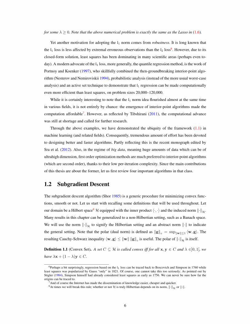
1.2 Subgradient Descent
The subgradient descent algorithm (Shor 1985) is a generic procedure for minimizing convex func-
tions, smooth or not. Let us start with recalling some definitions that will be used throughout. Let
our domain be a Hilbert space8 H equipped with the inner product 〈·, ·〉 and the induced norm ‖·‖H.
Many results in this chapter can be generalized to a non-Hilbertian setting, such as a Banach space.
We will use the norm ‖·‖H to signify the Hilbertian setting and an abstract norm ‖·‖ to indicate
the general setting. Note that the polar (dual norm) is defined as ‖g‖ = sup‖w‖≤1 〈w,g〉. The
resulting Cauchy-Schwarz inequality 〈w,g〉 ≤ ‖w‖ ‖g‖ is useful. The polar of ‖·‖H is itself.
Definition 1.1 (Convex Set). A set C ⊆ H is called convex iff for all x,y ∈ C and λ ∈]0, 1[, we
have λx + (1− λ)y ∈ C.
6Perhaps a bit surprisingly, regression based on the l1 loss can be traced back to Boscovich and Simpson in 1760 whileleast squares was popularized by Gauss “only” in 1821. Of course, one cannot take this too seriously: As pointed out byStigler (1984), Simpson himself had already considered least squares as early as 1756. We can never be sure how far theorigins can be traced to.
7And of course the Internet has made the dissemination of knowledge easier, cheaper and quicker.8At times we will break this rule; whether or notH is truly Hilbertian depends on its norm, ‖·‖H or ‖·‖.
6

Definition 1.2 (Convex Function). A function F : H → R ∪ ∞ is called σ-strongly convex w.r.t.
the norm ‖·‖ (not necessarily the induced Hilbertian norm) iff for all x,y ∈ H and λ ∈]0, 1[, we
have
F (λx + (1− λ)y) ≤ λF (x) + (1− λ)F (y)− σ2λ(1− λ) ‖x− y‖2 .
In the case σ = 0, we simply call F convex (in which case the norm ‖·‖ is irrelevant). In particular,
F is σ-strongly convex w.r.t. the Hilbertian norm ‖·‖H iff F − σ2 ‖·‖
2H is convex9.
The convention to let F take the value∞ for points outside of its domain proves to be convenient.
For instance, we can identify a convex set C with the indicator function
ιC(x) =
0, if x ∈ C∞, otherwise
. (1.8)
Under this convention, domF := x ∈ H : F (x) < ∞ signifies the (effective) domain, which is
necessarily a convex set if F is a convex function. To exclude triviality, we will only consider proper
functions—those with nonempty domain. For regularity purpose, we assume the convex function F
is closed, i.e. lower semicontinuous10. Collectively we use Γ0(H), or simply Γ0 if no confusion is
caused, to denote the set of all closed proper convex functions. The subdifferential of the convex
function F at point x is defined as the set
∂F (x) := g ∈ H : F (y) ≥ F (x) + 〈y − x,g〉 ,∀y, (1.9)
which is empty if x 6∈ domF . Note that the subdifferential is always a (weak*) closed convex set,
possibly containing more than one element. For instance, as readily verified from the definition, the
subdifferential of the absolute function | · | at origin is the interval [−1, 1]. It is also possible to have
empty subdifferential at some boundary points: An example would be the subdifferential at origin
of the function −√x defined on x ≥ 0. Notably, as long as F is continuous (and finite-valued) at
x, it can be shown that the subdifferential ∂F (x) is nonempty (Zalinescu 2002, Theorem 2.4.12), in
which case, any element in ∂F (x) is called a subgradient of F at the point x. It is also known that
F is differentiable at w iff ∂F (w) contains exactly one element, in which case we use the notation
∇F (w). A very useful rule, which is also easily verified from the definition of subdifferential, is
that
w? ∈ argminw
F (w) ⇐⇒ 0 ∈ ∂F (w?). (1.10)
Subgradient descent is an extremely simple iterative algorithm. Instantiating to (1.1), each itera-
tion amounts to11
wt+1 = PC(wt − ηt · gt), (1.11)
9This convenient rule, as a direct consequence of the underlying inner product, is no longer true for an abstract norm.10The function F : H → R ∪ ∞ is lower semicontinuous iff its sublevel set w ∈ H : F (w) ≤ α is closed for all
α ∈ R.11Throughout the thesis we use bold letters to denote vectors. Note that the i-th entry of w is denoted as wi, while wi is
some vector that may have nothing to do with w.
7

where ηt ≥ 0 is the step size, gt ∈ ∂F (wt), assuming the latter is nonempty, and
PC(z) := argminw∈C
12 ‖w − z‖2H (1.12)
is the Hilbertian projection onto the set C, assumed to be closed and convex here. In the case where
C is the whole space, we simply have PC(z) = z.
Under mild conditions on the objective function and the step size, we can supply the following
convergence analysis for the subgradient algorithm:
Theorem 1.1. Assume that the set C ⊆ H is closed convex and the objective F ∈ Γ0 has nonempty
(uniformly) bounded subdifferential12, that is, ‖g‖H ≤ M for all g ∈ ∂F (w),w ∈ C. Start with
w0 ∈ C, then after T iterations of the subgradient update (1.11), for any w ∈ C,
min0≤t≤T−1
F (wt)− F (w) ≤ ‖w0 −w‖2H +M2∑T−1t=0 η2
t
2∑T−1t=0 ηt
. (1.13)
Proof. The proof is simple and well-known, and we include it here for completeness. According to
the update rule (1.11):
‖wt+1 −w‖2H = ‖PC(wt − ηtgt)−w‖2H% w ∈ C % = ‖PC(wt − ηtgt)− PC(w)‖2H
% projections are nonexpansive % ≤ ‖wt − ηtgt −w‖2H= ‖wt −w‖2H + η2
t ‖gt‖2H − 2ηt 〈wt −w,gt〉 (1.14)
% gt is a subgradient, ηt ≥ 0 % ≤ ‖wt −w‖2H + η2t ‖gt‖2H + 2ηt(F (w)− F (wt))
% ∂F is bounded by M % ≤ ‖wt −w‖2H + η2tM
2 + 2ηt(F (w)− F (wt)). (1.15)
The lines with % · · ·% are used in the proof as “hints” or comments.
Telescoping we obtain
‖wT −w‖2H ≤ ‖w0 −w‖2H +M2T−1∑t=0
η2t + 2 max
0≤t≤T−1(F (w)− F (wt)) ·
T−1∑t=0
ηt.
Thus
min0≤t≤T−1
F (wt)− F (w) ≤ ‖w0 −w‖2H +M2∑T−1t=0 η2
t
2∑T−1t=0 ηt
,
as claimed.
Clearly, for the right-hand side of (1.13) to converge to 0, it is both sufficient and necessary13 to
have∑t ηt = ∞, ηt → 0. It is also possible to use a constant step size if we only desire some ε
accuracy.
12For finite-valued F , this condition is equivalent to F being M -Lipschitz continuous (w.r.t. the norm ‖·‖H), that is,|F (x)− F (y)| ≤M · ‖x− y‖H for all x,y ∈ H.
13Necessity: Vanishing of the first term requires∑t ηt = ∞ while vanishing of the second term, using the Cauchy-
Schwarz inequality, implies 1T
∑T−1t=0 ηt → 0, which is equivalent as ηt → 0 (since ηt ≥ 0). Sufficiency: For t sufficiently
large η2t ≤ εηt due to ηt → 0.
8

Corollary 1.1. Fix ε > 0, w0 ∈ C, and set ηt ≡ c/M2 · ε for some constant c ∈]0, 2[, then under
the assumptions of Theorem 1.1, after at most T =M2‖w0−w‖2H
c(2−c) · 1ε2 iterations of the subgradient
update (1.11), there exists some 0 ≤ t ≤ T − 1 such that
F (wt)− F (w) ≤ ε.
The same claim holds for the averaged iterate wT = 1T
∑T−1t=0 wt.
Some remarks about the subgradient algorithm are in order.
Remark 1.1 (Stochastic Setting). Let us mention that the subgradient algorithm is robust to noise,
in the sense that an unbiased estimate of the subgradient in each iteration suffices: simply take
expectation in (1.14), conditioned on wt (Nemirovski et al. 2009). A high probability bound is also
possible, see Remark 1.8 below for a more general result. Duchi et al. (2012) further studied the
case where the samples are not independent but sufficiently mixing.
Remark 1.2 (Online Setting). In online learning, the objective F is allowed to change in each
iteration. As a compensation, we evaluate the algorithm through the regret
RT (w) :=
T−1∑t=0
Ft(wt)− Ft(w), (1.16)
i.e. the algorithm competes with a single fixed point w in hindsight. Starting from (1.15) and setting
ηt ∝ 1/√t, it easily follows that the subgradient algorithm suffers only O(
√T ) regret (Zinkevich
2003). This rate can be proven optimal by considering C = [−1, 1], Ft(w) := Xt ·w, where Xt are
i.i.d. Bernoulli random variables (Hazan et al. 2007).
Remark 1.3 (Non-Hilbertian Setting). Sometimes it is important to consider the non-Hilbertian
structure in our problem. For this we replace the distance function d(x,y) = 12 ‖x− y‖2H with the
more general Bregman divergence (Bregman 1967), induced by a strongly convex Legendre function.
Definition 1.3. The function d is called Legendre if (a) C = int(dom d) is nonempty14; (b) d is
differentiable on C; and (c) ‖∇F (w)‖ →∞ as w approaches the boundary of C.
Definition 1.4. The 1-strongly convex Legendre function d induces the Bregman divergence
Dd(x,w) = d(x)− d(w)− 〈x−w,∇d(w)〉 . (1.17)
When the underlying function d is clear from context or simply unimportant, we use the short hand
D. Due to 1-strong convexity of d,
D(x,w) ≥ 12 ‖x−w‖2 ≥ 0, (1.18)
14We use int to denote the interior of a set, that is, the largest open subset.
9

and in particular D(x,w) = 0 iff x = w, see e.g. Yu (2013c). Take d = 12 ‖·‖
2H we recover the
usual distance function, although in general D need not be symmetric (nor jointly convex in its two
arguments). The generalized Pythagorean inequality
Dd(x,y) = Dd(x,w) + Dd(w,y)− 〈x−w,∇d(y)−∇d(w)〉 (1.19)
is easily verified.
The following lemma, which we learned from Tseng (2008), is very useful. (Note that as usual,
both ` and f belong to Γ0, the set of all closed proper convex functions.)
Lemma 1.1. Let w+ ∈ argminw `(w) + f(w) and assume f is differentiable15 at w+, then
`(w) + f(w) ≥ `(w+) + f(w+) + Df (w,w+). (1.20)
Proof. Indeed, (1.20) is exactly the optimality condition for w+: Due to the minimality of w+, we
have 0 ∈ ∂(`+ f)(w+), whereas the latter is equal to ∂`(w+) +∇f(w+), due to the differentiable
assumption of f at w+. Thus (1.20) follows from the convexity of `.
Despite the directness of Lemma 1.1, we will repeatedly need it in most proofs of this chapter.
The function f in Lemma 1.1 may oftentimes be itself a Bregman divergence (with a fixed second
argument), however, notice that the Bregman divergence induced by a Bregman divergence is itself.
Now we are ready to generalize the subgradient algorithm to non-Hilbertian settings. Recall that
the subgradient update can be concisely written as16
wt+1 = argminw∈C
F (wt) + 〈w −wt, ∂F (wt)〉+ 12ηt‖w −wt‖2H ,
i.e. we linearize the objective F at the current iterate wt and add a quadratic regularization to avoid
moving too far away (so that the linearization remains accurate). Quite naturally, we replace the
distance function with a Bregman divergence, yielding the mirror descent (MD) algorithm (Beck and
Teboulle 2003)17:
wt+1 = argminw∈C
F (wt) + 〈w −wt, ∂F (wt)〉+ 1ηtD(w,wt). (1.21)
The analysis of MD is very similar to what we had in the proof of Theorem 1.1. Indeed, applying
Lemma 1.1 to (1.21):
〈w, ∂F (wt)〉+ 1ηtD(w,wt) ≥ 〈wt+1, ∂F (wt)〉+ 1
ηtD(wt+1,wt) + 1
ηtD(w,wt+1).
15This technical assumption can be relaxed to ∂(` + f)(w+) = ∂`(w+) + ∂f(w+), which is exactly what is neededin the proof. When f is only subdifferentiable at w+, the induced Bregman divergence is somewhat arbitrary, however, thisgenerality is still useful since sometimes the induced “arbitrary” Bregman divergence appears only as an intermediate proofmeans.
16At times, we will abuse the notation ∂F as an arbitrary subgradient.17With w0 ∈ int(dom d), the iterates of MD will remain in int(dom d), for otherwise∇d(wt) will blow up (recall that
D is induced by some Legendre function d). Therefore D(w,wt) is always well-defined.
10

Using the convexity of F , (1.18), and rearranging:
ηt[F (wt)− F (w)] ≤ ηt 〈wt −wt+1, ∂F (wt)〉 − D(wt+1,wt)− D(w,wt+1) + D(w,wt)
≤ ηt ‖wt −wt+1‖ · ‖∂F (wt)‖ − 12 ‖wt+1 −wt‖2
− D(w,wt+1) + D(w,wt)
≤ η2t ‖∂F (wt)‖2
2− D(w,wt+1) + D(w,wt).
Putting a (uniform) upper bound on ‖∂F (wt)‖, we can telescope as before. Needless to say that
the same proof yields again an O(√T ) regret in the online setting.
Remark 1.4 (Strongly Convex Setting). Additionally, if F is σ-strongly convex, then the rate can be
improved (Hazan et al. 2007). Indeed, by the help of the characterization of strong convexity (see,
e.g. Yu (2013c))
F (x) ≥ F (w) + 〈x−w, ∂F (w)〉+ σ2 ‖x−w‖2 , (1.22)
in the Hilbertian setting we have from (1.14)
‖wt+1 −w‖2H ≤ ‖wt −w‖2H + η2t ‖gt‖2H + 2ηt(F (w)− F (wt))− ηtσ ‖w −wt‖2H .
Set ηt = 1σ(t+1) and telescope we obtain the improved M2(log T+1)
2σT rate (independent of ‖w0 −w‖H).
The log factor can be removed after a slight modification of the algorithm (Lacoste-Julien et al.
2012; Rakhlin et al. 2012). Note that the improved rate relies on the exact choice of the step size1σt , which requires the knowledge of σ. Unfortunately, an over-estimate of σ can lead to disastrous
results (Nemirovski et al. 2009, p. 1578).
For MD, there is an unfortunate mismatch between the norm ‖·‖ in the definition of strong
convexity (cf. (1.22)) and the Bregman divergence. It is not clear if we can still get an improved rate,
unless we modify the algorithm, see Remark 1.7 below for a detailed discussion.
Surprisingly, in black-box optimization, where the only information we can obtain is the func-
tion value and an arbitrary subgradient at any queried point, theO(1/ε2) complexity bound in Corol-
lary 1.1 cannot be improved (Nesterov 2003, Theorem 3.2.1), thereby justifying the optimality of the
subgradient method for generic nonsmooth convex optimization. On the other hand, the subgradient
algorithm completely ignores the composite structure in (1.1), and we will see in the next section
that by exploiting this structure (as opposed to black-box optimization), we can improve the rate
significantly.
1.3 Proximal Gradient
In this section we consider another first order algorithm that significantly improves the optimal
O(1/ε2) complexity of subgradient descent. Of course, that is possible only under additional as-
sumptions. Specifically, we need
11

Assumption 1.1. The objective F is in the composite form (1.1), i.e., F = ` + f for some (closed,
proper) convex functions ` and f .
Assumption 1.2. The component ` is differentiable (on the interior of dom `), and there exists some
finite constant L ≥ 0 such that the gradient ∇` satisfies the following inequality for all w,w′ ∈dom ` (w.r.t. some norm ‖·‖):
`(w) ≤ `(w′) + 〈w −w′,∇`(w′)〉+ L2 ‖w −w′‖2 . (1.23)
The inequality (1.23) simply means that the function ` can be upper bounded by a quadratic
function. Clearly if (1.23) holds for some L, then it also holds for all L ≥ L. Moreover, it is known
that (1.23) holds when the gradient ∇` is L-Lipschitz continuous (w.r.t. the dual norm ‖·‖)18, see
e.g. Zalinescu (2002, Corollary 3.5.7).19 Another convenient rule to check (1.23) for twice differ-
entiable `, in the Hilbertian setting, is that the eigenvalues of its Hessian are upper bounded by L
(Nesterov 2003, Theorem 2.1.6). Both the least squares loss (in Example 1.4) and the logistic loss
(1.3) satisfy Assumption 1.2.
The proximal gradient (PG) algorithm, first proposed by Fukushima and Mine (1981) as a lin-
earization (and also generalization if we let ` ≡ 0) of the proximal point algorithm (Martinet 1970;
Rockafellar 1976) in the Hilbertian setting, is also iterative. We will motivate PG from an opera-
tor splitting point of view as follows. First recall the optimality condition (1.10) for (1.1), under
Assumption 1.1 and Assumption 1.2:
0 ∈ ∇`(w?) + ∂f(w?), (1.24)
where w? is some assumed minimizer. That is, we are looking for an “annihilator” of the sum of two
operators: ∇` and ∂f . It follows from simple algebra that w? − η · ∇`(w?) ∈ (Id + η · ∂f)(w?),
where Id denotes the identity map. Thus20
w? = (Id + η · ∂f)−1(w? − η · ∇`(w?)). (1.25)
So we have arrived at a fixed-point equation, which also splits the two operators into two consecutive
steps. Quite naturally, with some initial point, we can repeatedly apply the fixed-point equation.
Hopefully the generated sequence will converge to a minimizer.
PG exactly realizes the above fixed-point iteration. It simply aims at minimizing the quadratic
upper bound in (1.23), with the regularizer untouched:
wt+1 = argminw
`(wt) + 〈w −wt,∇`(wt)〉+ 12ηt‖w −wt‖2H + f(w). (1.26)
18Meaning that ‖∇`(x)−∇`(y)‖ ≤ L · ‖x− y‖ for all x,y ∈ H.19Many references including Zalinescu (2002) require ` to be finite-valued, but the proof trivially extends to infinite-valued
`. The converse, that is, (1.23) implies the Lipschitz continuity of∇` in the case where ` is convex, seems to require ` to befinite-valued.
20It is not entirely obvious why we get equality here. For the sake of motivation, let us not dwell on rigor.
12

For clarity, let us decompose the above into two steps:
zt = wt − ηt∇`(wt), (1.27)
wt+1 = Pηtf (zt) := argminw
12ηt‖w − zt‖2H + f(w). (1.28)
The equivalence to the fixed-point equation (1.25) is verified by applying the optimality condition
(1.10) to (1.28). Note that by possibly redefining f we can assume that the constraint set C is the
whole space. The first step is a simple gradient update, taking only the smooth part ` into account;
the second step is simply the proximal map (Moreau 1965) of the other part f . The proximal map
has many interesting properties, some of which will be thoroughly discussed later. For now, it is
enough to notice that when f = ιC , the 0,∞-valued indicator function of the closed convex set
C, the proximal map reduces exactly to the Hilbertian projection onto C, in which case we recover
the projected gradient algorithm of Goldstein (1964).
The proximal gradient algorithm has been extensively studied in recent years, see e.g. (Beck
and Teboulle 2009a; Combettes and Wajs 2005; Nesterov 2013; Tseng 2008, 2010) and the many
references therein. In particular, we have the following convergence result:
Theorem 1.2. Let Assumption 1.1, Assumption 1.2 hold and assume further that dom ` ⊇ dom f .
Start with w0 ∈ dom f and choose some constant step size ηt ≡ η ∈]0, 1/L[. Then for any w,
F (wt) ≤ F (w) +‖w0 −w‖2H
2ηt.
Proof. Let w ∈ domF be arbitrary, then by the smoothness assumption on `:
F (wt+1) = f(wt+1) + `(wt+1)
% inequality (1.23) % ≤ f(wt+1) + `(wt) + 〈wt+1 −wt,∇`(wt)〉
+ 12ηt‖wt+1 −wt‖2H (1.29)
% (1.27), (1.28) and Lemma 1.1 % ≤ f(w) + `(wt) + 〈w −wt,∇`(wt)〉+ 12ηt‖w −wt‖2H
− 12ηt‖w −wt+1‖2H (1.30)
% ` is convex % ≤ f(w) + `(w) + 12ηt‖w −wt‖2H − 1
2ηt‖w −wt+1‖2H .
(1.31)
Now use a constant step size ηt ≡ η and we can telescope:
T−1∑t=0
[F (wt+1)− F (w)] ≤ 12η ‖w −w0‖2H .
Substitute w with wt in (1.31) we obtain the monotonic property: F (wt+1) ≤ F (wt). Thus
T · [F (wT )− F (w)] ≤T−1∑t=0
[F (wt+1)− F (w)] ≤ 12η ‖w0 −w‖2H ,
as claimed.
13

Needless to say that the same rate holds in the special case f = ιC for some closed and convex
set C, corresponding to the projected gradient algorithm of Goldstein (1964). On the other hand, the
current analysis (and rate) of PG can not be extended to the stochastic or online setting: the inequality
(1.29) breaks down. However, as we will see in Section 1.4, a parallel analysis and a slower rate
such as that of the subgradient algorithm can be achieved. On the flip side, PG is significantly faster:
O(1/ε) versus the O(1/ε2) complexity of the subgradient descent, cf. Corollary 1.1, provided that
we can very quickly compute the proximal map (1.28) in each iteration. Such is the case when the
regularizer f is “simple”—a point can be easily made by revisiting the LASSO example; for more
examples, see Combettes and Pesquet (2011), Bach et al. (2011, §3.3), Parikh and Boyd (2013, §6).
Example 1.4 (continuing from p. 3). Clearly, both Assumption 1.1 and Assumption 1.2 are satisfied
in this example. The first step of PG is easy:
zt = wt − ηX>(Xwt − y).
The second step, known as the soft-thresholding or shrinkage operator, can be computed in closed-
form:
[Pηλf (z)]i = [Pληf (z)]i = zi(1− λη/|zi|
)+. (1.32)
See Figure 1.4 for a one dimensional example (with the understanding ηλ = µ). There, Mµf , the
Moreau envelop, is the attained minimal function value on the right-hand side of (1.28). In this
case,
Mµf (z) =
12µz
2, if |z| ≤ µ|z| − µ
2 , otherwise
coincides with the so-called Huber’s loss in robust statistics (Huber 1964).
PG, in this specific form with l1 norm regularization, appeared first in Starck et al. (2003) and
Figueiredo and Nowak (2003), although its formal convergence was established later in Daubechies
et al. (2004). Surprisingly, Daubechies et al. (2004) actually proved strong21 convergence while it
was known that PG, in general, may fail to converge strongly (Güler 1991). Further improvement
can be found in Combettes and Pesquet (2007). In the finite dimensional setting, Tseng (2010) proved
that in fact PG (on this example) eventually converges under a geometric progression after an un-
specified number of steps.
Example 1.4 also reveals a nice property about the proximal gradient algorithm. First recall that
the regularizer f in machine learning is usually employed for realizing useful structural priors on the
parameters. As we will show later, there is a 1-1 correspondence between the regularizer f and its
proximal map Pηf . Therefore the nice properties of the regularizer f may be reflected in its proximal
21By strong convergence we mean the usual convergence under the norm, which is to be contrasted with the “weak”convergence induced by all continuous linear functionals. The two are the same in a finite dimensional space but differfundamentally in infinite dimensional spaces.
14

−2 −1.5 −1 −0.5 0 0.5 1 1.5 2−1
−0.5
0
0.5
1
1.5
2η = 1
f = | · |
Mη
f =Hube r
Pη
f =Shrinkage
Figure 1.4: The Moreau envelop and the proximal map of the absolute function | · |.
map, thus easily exploited by PG. Back to Example 1.4, the l1 norm regularizer is utilized to promote
sparsity; indeed its proximal map shrinks small components to zero. This feature is in sharp contrast
with the generic subgradient method which does not produce sparse intermediate iterates, thus partly
explains why PG, besides its fast convergence, is so popular in machine learning applications.
Very surprisingly, the rate of PG is not optimal and a slight modification of the algorithm could
further improve it to O(1/√ε). The first variant along this direction is due to Beck and Teboulle
(2009a) although the main idea traces back to Nesterov (1983). Following Tseng (2008), we call
these fast variants accelerated proximal gradient (APG). In particular, the algorithm of Beck and
Teboulle (2009a), widely known as FISTA (Fast Iterative Shrinkage-Thresholding Algorithm), is
given in Algorithm 1, and we summarize its convergence property in the next theorem.
Theorem 1.3. Under Assumption 1.1, Assumption 1.2, and assume dom ` ⊇ 2w −w′ : w,w′ ∈dom f. Start with w0 ∈ domF and let w be arbitrary. The iterates produced by Algorithm 1
satisfy
F (wt+1) ≤ F (w) +2L ‖w0 −w‖2H
(t+ 1)2.
Proof. We learned the following inspiring proof from Tseng (2010). First note that by Assump-
tion 1.2 and Lemma 1.1,
F (wt+1) ≤ f(wt+1) + `(ut+1) + 〈wt+1 − ut+1,∇`(ut+1)〉+ L2 ‖wt+1 − ut+1‖2H
≤ f(v) + `(ut+1) + 〈v − ut+1,∇`(ut+1)〉+ L2 ‖v − ut+1‖2H − L
2 ‖v −wt+1‖2H≤ f(v) + `(v) + L
2 ‖v − ut+1‖2H − L2 ‖v −wt+1‖2H . (1.33)
Now to get a faster convergence, we need to somehow make the Lipschitz constant smaller as t →∞. This is achieved by choosing the convex combination vt = (1 − 1
γt+1)wt + 1
γt+1w for some
arbitrary w ∈ domF , and γt+1 ≥ 1 is specified as line 5 of Algorithm 1. Plug into (1.33) we obtain
F (wt+1) ≤ F ((1− 1γt+1
)wt + 1γt+1
w) + L2
∥∥∥(1− 1γt+1
)wt + 1γt+1
w − ut+1
∥∥∥2
H
15

Algorithm 1 FISTA (Beck and Teboulle 2009a).1: Initialize: w0 = u1 ∈ domF , η = 1/L, γ1 = 1.2: for t = 1, 2, . . . do3: zt = ut − η∇`(ut)4: wt = Pηf (zt)
5: γt+1 =1+√
1+4γ2t
2
6: ut+1 = wt + γt−1γt+1
(wt −wt−1)
7: end for
− L2
∥∥∥(1− 1γt+1
)wt + 1γt+1
w −wt+1
∥∥∥2
H≤ (1− 1
γt+1)F (wt) + 1
γt+1F (w) + L
2γ2t+1‖w −wt + γt+1(wt − ut+1)‖2H
− L2γ2t+1‖w −wt + γt+1(wt −wt+1)‖2H . (1.34)
Define st := wt−γt+1(wt−ut+1). Due to the ingenious choice of ut+1 (in line 6 of Algorithm 1),
it follows from simple algebra that wt − γt+1(wt −wt+1) = st+1, thus
F (wt+1)− F (w) ≤ (1− 1γt+1
)[F (wt)− F (w)] + L2γ2t+1
[‖w − st‖2H − ‖w − st+1‖2H
].
Using the relation22 γ2t = γ2
t+1 − γt+1, we obtain the recursion
γ2t+1[F (wt+1)− F (w)] + L
2 ‖w − st+1‖2H ≤ γ2t [F (wt)− F (w)] + L
2 ‖w − st‖2H .
Since γ1 = 1 we can set γ0 = 0. Also s0 = w0, hence
F (wt+1)− F (w) ≤ L2γ2t+1‖w0 −w‖2H .
The proof is complete once we notice by induction that γt ≥ t+12 .
It is quite remarkable that a simple extrapolation of the iterates wt (line 6 in Algorithm 1)
immediately boosts the convergence rate from O(1/ε) to O(1/√ε), although a clear intuitive ex-
planation is not available. We note that Algorithm 1 requires the smooth part ` to be defined on
2w −w′ : w,w′ ∈ dom f as the extrapolation (line 6 in Algorithm 1) may go outside of dom f
(whereas line 4 in Algorithm 1 guarantees wt ∈ dom f ). There are other variants that avoid this
issue, see Remark 1.6 below, and Tseng (2008) for more discussions.
When the Lipschitz constantL is not known in advance, we can employ an adaptive backtracking
strategy, see Beck and Teboulle (2009a) and Nesterov (2013) for detailed discussions. Wright et al.
(2009) combined the line search procedure of Barzilai and Borwein (1988) with PG, and claimed
superior performance on some signal processing experiments.
Remark 1.5. We can also plug a local improver into each iteration of FISTA, without affecting its
convergence rate, see Algorithm 2. The only requirement on the subroutine Local is that F (wt) ≤22 If w ∈ argminF , then γ2t ≥ γ2t+1 − γt+1 is enough, in particular, the simpler rule γt = t+1
2can be used.
16

F (rt). Indeed, we can derive (1.34) again with minor changes:
F (rt+1) ≤ (1− 1γt+1
)F (wt) + 1γt+1
F (w) + L2γ2t+1‖w −wt + γt+1(wt − ut+1)‖2H
− L2γ2t+1‖w −wt + γt+1(wt − rt+1)‖2H .
As before, define st := wt − γt+1(wt − ut+1). Then we set ut+1 so that wt − γt+1(wt − rt+1) =
st+1. By our requirement on Local, F (wt+1) ≤ F (rt+1), therefore telescope as before we ob-
tain the same convergence rate as in Theorem 1.3. Clearly with wt ≡ rt we recover the original
FISTA; with F (wt) = minF (rt), F (wt−1) we recover the monotone FISTA of Beck and Teboulle
(2009b).
Algorithm 2 FISTA with local search.1: Initialize: w0 = r0 = u1 ∈ domF , η = 1/L, γ1 = 1.2: for t = 1, 2, . . . do3: zt = ut − η∇`(ut)4: rt = Pηf (zt)5: wt = Local(rt)
6: γt+1 =1+√
1+4γ2t
2
7: ut+1 = wt + γt−1γt+1
(wt −wt−1) + γtγt+1
(rt −wt)
8: end for
Remark 1.6. The generalization to non-Hilbertian settings is again possible. Indeed, to generalize
Theorem 1.2, we need only apply (1.18) to upper bound (1.29) with the Bregman divergence, and
then apply Lemma 1.1 to (1.30).
The proof of Theorem 1.3 exploited some special property of the norm ‖·‖H (e.g. pulling out
the scalar 1/γt+1), therefore cannot be directly generalized. However, a slight modification suffices.
Indeed, consider the iteration
vt = (1− 1γt+1
)wt + 1γt+1
ut (1.35)
ut+1 = argminu〈u− vt,∇`(vt)〉+ f(u) + L
γt+1D(u,ut) (1.36)
wt+1 = (1− 1γt+1
)wt + 1γt+1
ut+1, (1.37)
where the iterate vt, appearing implicitly in the proof of Theorem 1.3, has been made explicit. By
Assumption 1.2; convexity of f , (1.35) and (1.37); (1.18); (1.36) and Lemma 1.1; convexity of `; we
get the following chain of inequalities:
F (wt+1) ≤ f(wt+1) + `(vt) + 〈wt+1 − vt,∇`(vt)〉+ L2 ‖wt+1 − vt‖2
≤ (1− 1γt+1
)[f(wt) + `(vt) + 〈wt − vt,∇`(vt)〉]
+ 1γt+1
[f(ut+1) + `(vt) + 〈ut+1 − vt,∇`(vt)〉] + L2γ2t+1‖ut+1 − ut‖2
≤ (1− 1γt+1
)[f(wt) + `(vt) + 〈wt − vt,∇`(vt)〉]
+ 1γt+1
[f(ut+1) + `(vt) + 〈ut+1 − vt,∇`(vt)〉] + Lγ2t+1
D(ut+1,ut)
17

Algorithm 3 PSG (Duchi and Singer 2009).1: Initialize: w0 ∈ argmin f , η0 ≥ 0.2: for t = 0, 1, . . . do3: wt+1 = argminw 〈w −wt, ∂`(wt)〉+ 1
2ηt‖w −wt‖2H + f(w)
4: = Pηtf(wt − ηt · ∂`(wt)
)5: end for
≤ (1− 1γt+1
)[f(wt) + `(vt) + 〈wt − vt,∇`(vt)〉]
+ 1γt+1
[f(w) + `(vt) + 〈w − vt,∇`(vt)〉] + Lγ2t+1
D(w,ut)− Lγ2t+1
D(w,ut+1)
≤ (1− 1γt+1
)F (wt) + 1γt+1
F (w) + Lγ2t+1
D(w,ut)− Lγ2t+1
D(w,ut+1).
Set γt as in line 6 of Algorithm 1. Telescope as before, we obtain
F (wt+1) ≤ F (w) +4LD(w,u0)
(t+ 1)2.
It might appear that APG should always be preferred over PG, since it enjoys a faster conver-
gence rate which are usually confirmed in practice. However, experience warns us of drawing any
conclusion of this type. Indeed, the additional extrapolation step in APG makes analyzing its iterates
(instead of the function value as done in Theorem 1.3) much more difficult. In contrast, under fairly
loose conditions on the step size and the finite-valued assumption on `, it is easy to prove that the
iterates generated by PG converges (weakly) to some minimizer (Combettes and Wajs 2005).
1.4 Proximal Subgradient
The PG algorithm in the previous section replaces the Hilbertian projection in the projected gradient
algorithm of Goldstein (1964) with the more general proximal map (Moreau 1965). Straightfor-
wardly, it is tempting to recycle the same idea on the Hilbertian projection in the projected subgra-
dient algorithm that we saw in Section 1.2. The resulting algorithm simply abandons the smoothness
Assumption 1.2 and uses an arbitrary subgradient in the first step of PG. Consequently, we need to
adopt a diminishing step size (as the accuracy requirement ε goes to 0), and bear a slower rate of con-
vergence. The resulting Algorithm 3, which we call proximal subgradient (PSG), has been explicitly
studied by Duchi and Singer (2009). We record their result below.
Theorem 1.4. Under Assumption 1.1 and assume ‖g‖H ≤ M for all g ∈ ∂`(w) 6= ∅ and w ∈dom f . Use a constant step size ηt ≡ η and start with w0 ∈ dom f . Then after T iterations of the
proximal subgradient algorithm, we have for any w ∈ domF ,
T−1∑t=0
[F (wt)− F (w)] ≤ ‖w0 −w‖2H +M2η2T
2η+ f(w0)− f(wT ). (1.38)
Proof. The proof resembles the one in Theorem 1.1. Slightly abusing the notation to also denote
∂F (w) as the (particular) subgradient of F at w selected by the algorithm. Let w ∈ domF be
18

arbitrary. Apply Lemma 1.1 and rearrange,
‖wt+1 −w‖2H ≤ ‖wt −w‖2H + 2ηt[〈w −wt, ∂`(wt)〉+ f(w)− f(wt+1)]
+ 2ηt 〈wt −wt+1, ∂`(wt)〉 − ‖wt+1 −wt‖2H (1.39)
% convexity of ` % ≤ ‖wt −w‖2H + 2ηt[f(w)− f(wt+1) + `(w)− `(wt)]
+ 2ηt 〈wt −wt+1, ∂`(wt)〉 − ‖wt+1 −wt‖2H (1.40)
% ∂` is bounded by M % ≤ ‖wt −w‖2H + 2ηt[f(w)− f(wt+1) + `(w)− `(wt)] + η2tM
2.
For simplicity choose a constant step size ηt ≡ η we can telescope:
T−1∑t=0
[f(wt+1)− f(w)] +
T−1∑t=0
[`(wt)− `(w)] ≤ ‖w0 −w‖2H +M2η2T
2η.
Rearrange, we obtain the claim (1.38).
If one is concerned with the last term f(w0) − f(wT ), we can remove it by starting from
w0 ∈ argmin f .
Dealing with a natural generalization of the projected subgradient method (cf. Section 1.2), we
expect to obtain the same, if not worse, rate of convergence for PSG. The next corollary indeed
confirms this, hence also demonstrates that the composite structure (1.1) alone can not lead to faster
rates. Note that an efficient implementation of PSG hinges on our ability to quickly solve the proxi-
mal map in line 4 of Algorithm 3—a requirement usually stronger than getting an arbitrary subgra-
dient of f . The flip side of not linearizing f in line 3 of Algorithm 3 is the possibility to explicitly
leverage any special property of the proximal map of the regularizer f , such as the sparsity we saw
in Example 1.4.
Corollary 1.2. Fix ε > 0. Choose w0 ∈ argmin f and set η ≡ c/M2 · ε for some constant c ∈]0, 2[.
Then, under the assumptions of Theorem 1.4, after at most T =M2‖w0−w‖2H
c(2−c) · 1ε2 iterations, there
exists some 0 ≤ t ≤ T − 1 such that
F (wt) ≤ F (w) + ε.
The same claim holds for the averaged iterate wT = 1T
∑T−1t=0 wt.
Remark 1.7. In order to obtain a faster rate in the presence of strong convexity, as mentioned
previously in Remark 1.4, we follow Duchi et al. (2010) to (slightly) strengthen the definition of
σ-strong convexity (w.r.t. h) to
g(w′) ≥ g(w) + 〈w′ −w, ∂g(w)〉+ σDh(w′,w), (1.41)
where h is 1-strongly convex in the usual sense. Note that the new definition of strong convexity is
trivially satisfied when Dg = σDh, say g = σh. We replace the distance ‖·‖H in Algorithm 3 by the
Bregman divergence Dh(·, ·).
19

When ` is σ-strongly convex in the above sense, we improve (1.40) to
Dh(w,wt+1) ≤ Dh(w,wt) + ηt[f(w)− f(wt+1) + `(w)− `(wt)− σDh(w,wt)] +η2tM
2
2 .
Use the smaller step size ηt = 1σ(t+1) and telescope; we obtain the same rate M2(log T+1)
2σT as before.
When f is σ-strongly convex in the above sense, by Lemma 1.1 we improve23 (1.39) to
Dh(w,wt+1) ≤ Dh(w,wt) + ηt[f(w)− f(wt+1) + `(w)− `(wt)− Df (w,wt+1)] +η2tM
2
2
≤ Dh(w,wt) + ηt[f(w)− f(wt+1) + `(w)− `(wt)− σDh(w,wt+1)] +η2tM
2
2 .
Use again ηt = 1σ(t+1) and telescope; we obtain the similar rate 2σ2Dh(w,w0)+M2(log T+1)
2σT .
Remark 1.8. Needless to say that the same proof (for any Bregman divergence) works in the online
and stochastic setting. It is also easy to replace the bounded subdifferential assumption on ∂` with
the slightly more general one (Duchi et al. 2010): ‖∂`‖ ≤ a`+ b.
Next, we give a high probability bound for PSG when in each iteration we only have access to
an unbiased estimate, say Gt of the subgradient ∂`(wt). Reasoning as in (1.39),
D(w,wt+1) ≤ D(w,wt) + 2ηt[〈w −wt, Gt〉+ f(w)− f(wt+1)]
+ 2ηt 〈wt −wt+1, Gt〉 − D(wt+1,wt)
≤ D(w,wt) + 2ηt[〈w −wt, ∂`(wt)〉+ f(w)− f(wt+1)]
+ 2ηt[〈w −wt, Gt − ∂`(wt)〉 (1.42)
+ 2ηt 〈wt −wt+1, Gt〉 − D(wt+1,wt). (1.43)
Assuming ‖Gt‖ ≤ M , (1.43) can be dealt with as before. The term in (1.42), for a fixed w, is a
bounded martingale difference (Pinelis 1994), thus its cumulative sum highly concentrates around
its expected value, which is 0 due to the unbiasedness of Gt.
Remark 1.9. The whole point of PSG is not to linearize the regularizer f . Following Bach (2013b),
we now go against this philosophy in the case where f is σ-strongly convex (in the usual sense). As
a compensation, we employ the Bregman divergence induced by f itself. Specifically, consider the
iterate
wt+1 = argminw
`(wt) + f(wt) + 〈w −wt, ∂`(wt) + ∂f(wt)〉+ 1ηtDf (w,wt). (1.44)
Note that (1.44) is equally easy to solve as in PSG. By Lemma 1.1 24,
〈w −wt+1, ∂`(wt) + ∂f(wt)〉+ 1ηtDf (w,wt) ≥ 1
ηtDf (wt+1,wt) + 1
ηtDf (w,wt+1).
23In this case, we need f to be differentiable at each wt, see footnote 15 for some relaxation.24Again, see footnote 15 for some technical requirement. In particular, when f is nonsmooth, we need to be consistent
in choosing the subgradient such that ∂f(wt+1) = (1 − ηt)∂f(wt) − ηt∂`(wt). Here by ∂f we mean the particularsubgradient used in the algorithm, not the general subdifferential.
20

Algorithm 4 RDA (Xiao 2010).1: Initialize: w0 ∈ argmin f , g0 = 0, β0 > 0, αt ≡ 1.2: for t = 1, 2, . . . do3: gt−1 ∈ ∂`(wt−1)4: st = st−1 + αt−1gt−1
5: choose βt6: wt = argminw 〈w, st〉+ βt · D(w,w0) + (
∑tτ=0 ατ ) · f(w)
7: end for
The above, thanks to the (trivial) inequality (1.41) with g = f, h = f/σ, becomes
ηt(F (wt)− F (w)) ≤ ηt 〈∂F (wt),wt −wt+1〉 − Df (wt+1,wt)
+ (1− ηt)Df (w,wt)− Df (w,wt+1)
≤ η2t ‖∂F (wt)‖22σ + (1− ηt)Df (w,wt)− Df (w,wt+1).
Let ηt = 2t+2 , multiply t+1
ηton both sides, and telescope
T−1∑t=0
(t+ 1)(F (wt)− F (w)) ≤ −T (T+1)2 Df (w,wT+1) +
T−1∑t=0
t+ 1
t+ 2
‖∂F (wt)‖2σ
.
Assuming ‖∂F (wt)‖ ≤M uniformly in t, we obtain an O(1/T ) rate of convergence:
F
(2
T (T+1)
∑T−1
t=0(t+ 1)wt
)− F (w) ≤ 2M2
σ(T+1) .
Compared with Remark 1.7, we have managed to remove the log factor, under a slightly stronger
bounded subdifferential assumption. However, the current analysis, although works fine in the stochas-
tic setting, cannot be extended to the online setting, unless we are willing to modify the definition
of the regret. Surprisingly, Bach (2013b) showed, by comparing the iterates, that (1.44) is in fact
equivalent to the generalized condition gradient that we will study in Chapter 4, see Theorem 4.6
there. More analysis on similar step size rules can be found in Shamir and Zhang (2013).
1.5 Regularized Dual Averaging
The regularized dual averaging (RDA) of Xiao (2010), in some sense the “dual” of PSG, is a com-
posite generalization of the dual averaging proposed by Nesterov (2009). As summarized in Algo-
rithm 4, RDA averages the subgradients, instead of the iterates. We will motivate and present RDA
in a different way than Xiao (2010) or Nesterov (2009).
We need one more definition.
Definition 1.5. For any closed, proper and convex function F ∈ Γ0, its Fenchel conjugate F ∗ is
defined as:
F ∗(g) = supw〈w,g〉 − F (w). (1.45)
21

It is easily verified that again F ∗ ∈ Γ0. Moreover, (F ∗)∗ = F . From the definition we have the
inequality
〈g,w〉 ≤ F (w) + F ∗(g),
with equality iff w ∈ ∂F ∗(g) iff g ∈ ∂F (w).
By the Fenchel-Rockafellar duality (Zalinescu 2002, Corollary 2.8.5), we have the relation (un-
der mild technical conditions)
infw`(w) + f(w) = sup
g−`∗(g)− f∗(−g)
= − infg`∗(g)︸ ︷︷ ︸f(g)
+ supw〈w,−g〉 − f(w)︸ ︷︷ ︸
˜(g)
. (1.46)
In other words, we have transformed the original composite problem into a similar one in the dual,
with the role of ` and f swapped. Of course, we can now apply PSG on this dual formulation (1.46),
provided that we can compute the proximal map P1/ηt
f= P
1/ηt`∗ , which, as we will see in the next
chapter, is computationally equivalent to P1/ηt` . Said differently, we could have just swapped the
role of ` and f in the original problem—disappointingly—nothing seems to have been gained by
going to the dual. This is where we need a substantially new idea.
The idea is to apply a PG-like algorithm to the dual; more precisely, the generalized conditional
gradient (GCG) algorithm that we will thoroughly discuss in Chapter 4. GCG, like PG, requires the
loss ` to be smooth, i.e., satisfy Assumption 1.2. Unfortunately, ˜ in (1.46) usually is not smooth,
unless the regularizer f is strongly convex. Nevertheless, we can turn instead to a smooth approxima-
tion of ˜. Let w0 ∈ argmin f , take the Bregman divergence D(w,w0) (induced by some 1-strongly
convex function), and consider
˜µ(g) = sup
w〈w,−g〉 − f(w)− µ · D(w,w0), (1.47)
which, being the Fenchel conjugate of a µ-strongly convex function, satisfies Assumption 1.2 with
L = 1/µ, see, e.g. Zalinescu (2002, Corollary 3.5.11). Observe that (1.47) is exactly the step 6 in
Algorithm 4, up to a sign and constant change. GCG proceeds by linearizing the smooth loss ˜µ in
each step and finds a direction
argming〈g,−wt+1〉+ f(g) = argmax
g〈g,wt+1〉 − `∗(g) = ∂`(wt+1).
Then GCG simply takes a convex combination of the direction above and the current iterate, that is,
step 4 in Algorithm 4 (better seen if we consider the average st = st/∑tτ=0 ατ ). Note that when
f is itself σ-strongly convex for some σ > 0, ˜ is automatically smooth. In this case we use the
Bregman divergence induced by f itself, that is D = 1σDf .
To analyze the performance of RDA, we introduce the setQ := w : D(w,w0) ≤ ∆2 for some
∆ > 0. Since D is strongly convex, Q is bounded. We will compare the iterates of RDA with any
22

fixed point inQ—a restriction of the original problem. Obviously, as ∆ becomes large, we approach
the original problem. Note that Algorithm 4 does not need to know Q at all. The performance of
RDA , in the online setting, is summarized below.
Theorem 1.5. Under Assumption 1.1, assume that `t is subdifferentiable on dom f and f is σ-
strongly convex (w.r.t. the norm ‖·‖). Then for any w ∈ domF ∩ Q, Algorithm 4 with step size
(βt)t≥1 ↑ satisfies
T−1∑t=0
`t(wt) + f(wt)− `t(w)− f(w) ≤ βT∆2 +
T−1∑t=0
12(βt+σt)
‖gt‖2 . (1.48)
Proof. Note that by definition st :=∑t−1i=0 αigi. We upper bound the regret as follows:
RT (w) =
T−1∑t=0
αt[`t(wt) + f(wt)− `t(w)− f(w)]
% convexity of `t % ≤T−1∑t=0
αt[〈wt −w,gt〉+ f(wt)− f(w)]
% w ∈ Q % = 〈−wT , sT 〉 − (
T−1∑t=0
αt) · f(wT )− βTD(wT ,w0) +
T−1∑t=0
αt[〈wt,gt〉+ f(wt)]
+ [〈wT , sT 〉+ (
T−1∑t=0
αt)f(wT ) + βTD(wT ,w0)]
− [〈w, sT 〉+ (
T−1∑t=0
αt)f(w) + βTD(w,w0)] + βT∆2
% definition of wT , % = 〈−wT , sT 〉 − (
T−1∑t=0
αt) · f(wT )− βTD(wT ,w0)
% D(·, ·) and Lemma 1.1 % + βT∆2 − (βT + σ
T−1∑t=0
αt) · D(wT ,w) +
T−1∑t=0
αt[〈wt,gt〉+ f(wt)]
% (βt)t≥1 ↑ % ≤ 〈−wT , sT−1 + αT−1gT−1〉 − (
T−2∑t=0
αt) · f(wT )− βT−1D(wT ,w0)
− αT−1f(wT ) + βT∆2 +
T−1∑t=0
αt[〈wt,gt〉+ f(wt)]
− (βT + σ
T−1∑t=0
αt) · D(wT ,w)
≤ maxw〈−w, sT−1 + αT−1gT−1〉 − (
T−2∑t=0
αt) · f(w)− βT−1D(w,w0)
− αT−1f(wT ) + βT∆2 +
T−1∑t=0
αt[〈wt,gt〉+ f(wt)]
− (βT + σ
T−1∑t=0
αt) · D(wT ,w)
% (1.23) % ≤ maxw〈−w, sT−1〉 − (
T−2∑t=0
αt) · f(w)− βT−1D(w,w0)
23

+ 〈−wT−1, αT−1gT−1〉+‖αT−1gT−1‖2
2(βT−1+σ∑T−2t=0 αt)
− αT−1f(wT )
+ βT∆2 − (βT + σ
T−1∑t=0
αt) · D(wT ,w) +
T−1∑t=0
αt[〈wt,gt〉+ f(wt)]
% iterating the argument % ≤ 〈w0 −w1, α0g0〉 − β1D(w1,w0) + α0f(w0)− αT−1f(wT )
+ βT∆2 +
T−1∑t=1
‖αtgt‖22(βt+σ
∑t−1s=0 αs)
+
T−1∑t=1
(αt − αt−1)f(wt)
− (βT + σ
T−1∑t=0
αt) · D(wT ,w)
≤ (β0 − β1)D(w1,w0) + α0f(w0)− αT−1f(wT )
+ βT∆2 +
T−1∑t=0
‖αtgt‖22(βt+σ
∑t−1s=0 αs)
+
T−1∑t=1
(αt − αt−1)f(wt)
− (βT + σ
T−1∑t=0
αt) · D(wT ,w).
We need only consider σ 6= 0, in which case D = 1σDf . By definition
w1 = argminw
〈w, α0g0〉+ β1D(w,w0) + α0f(w)
and w0 ∈ argminw f(w). Therefore by Lemma 1.1,
〈w1, α0g0〉+ β1D(w1,w0) + α0f(w1) + α0Df (w0,w1) ≤ 〈w0, α0g0〉+ α0f(w0),
which upon simplification yields
(α0σ + β1)D(w1,w0) ≤ 〈w0 −w1, α0g0〉 ≤ ‖w0 −w1‖ ‖α0g0‖≤√
2D(w1,w0) ‖α0g0‖ .
Combing the bounds we obtain
RT (w) + (βT + σ
T−1∑t=0
αt) · D(wT ,w) ≤ βT∆2 +2(β0 − β1)
(α0σ + β1)2‖α0g0‖2 +
T−1∑t=0
‖αtgt‖22(βt+σ
∑t−1s=0 αs)
+α0f(w0)− αT−1f(wT ) +
T−1∑t=1
(αt − αt−1)f(wt).
Setting αt ≡ 1 and β0 = β1 completes the proof.
There is an apparent trade-off in the two terms on the right-hand side of (1.48), due to the
nondecreasing requirement on βt. A careful balance yields
Corollary 1.3. Let β0 = β1 = 1, βt+1 = βt + 1/βt, t ≥ 1 and βt = γβt, t ≥ 0, then under the
assumptions of Theorem 1.5 and assuming ‖gt‖ ≤ M, t ≥ 0, the regret of Algorithm 4 can be
bounded by
βT (γ∆2 +M2
2γ) ≤ (1/2 +
√2T − 1)(γ∆2 +
M2
2γ).
24

Proof. Simply verify by induction that βt+1 =∑tτ=0 1/βτ , t ≥ 0, and
√2t− 1 ≤ βt ≤ 1
1+√
3+
√2t− 1, t ≥ 1.
Therefore RDA suffers only O(√T ) regret, similar as PSG. If we let `t ≡ ` and choose ∆ ≥
‖w0 −w?‖ for some minimizer w? of (1.1), then RDA converges to the minimum value of (1.1).
Remark 1.10. The proof extends to the stochastic case where gt is only an unbiased estimate of
∂`(wt). The reason is clear: the smoothness of ˜µ, hence the inequality (1.23), is not impaired by
the noise in `.
Remark 1.11. If our “competitor” w is an interior point of Q, we can further bound the dual
variable st. Indeed, from the proof of Theorem 1.5 we have
maxz∈Q
T−1∑t=0
αt[〈wt − z,gt〉+ f(wt)− f(z)] =
T−1∑t=0
αt[〈wt −w,gt〉+ f(wt)− f(w)]
+ maxz∈Q〈w − z, sT 〉+ (
T−1∑t=0
αt) · (f(w)− f(z))
≥ RT (w) + maxz:‖z−w‖≤r
〈w − z, sT 〉+ (
T−1∑t=0
αt) · (f(w)− f(z))
≥ RT (w) + r ‖sT ‖ + (
T−1∑t=0
αt) · [−r ‖∂f(z)‖ + σ2 r
2],
where z satisfies 〈w − z, sT 〉 = ‖w − z‖ ‖sT ‖. Rearrange and notice that the left-hand side has
already being taken care of in the proof of Theorem 1.5.
1.6 Structured Sparsity
The four algorithms we discussed in the previous sections are by no means exhaustive. Other popular
alternatives in machine learning include coordinate gradient (Tseng and Yun 2009a,b), alternating
direction method of multipliers (Boyd et al. 2010), homotopy algorithms (Efron et al. 2004; Osborne
et al. 2000), averaging gradient (Blatt et al. 2007; Roux et al. 2012), randomized coordinate descent
(Nesterov 2012), mirror-prox (Baes et al. 2013; Nemirovski 2004) and possibly still others. A com-
mon requirement of many of these algorithms, in particular, the four we reviewed, is the possibility
of quickly solving the proximal map (1.28) in each iteration (recall that the Hilbertian projection
is a special proximal map). For the l1 norm which has played a vital role in sparse estimation, its
proximal map indeed can be easily computed, see Example 1.4. However, we quickly lose this nice
gift once we consider more refined notions of sparsity—structured sparsity (Bach et al. 2012).
Structured sparsity, generally speaking, refers to our belief that not all sparse patterns are equally
desired.25 Some particular sparse patterns may be preferred as compared to others, and sparsity
may present itself in other structured forms, in addition to the number of nonzero elements. Let us
consider some examples.25Which, by the way, should not be generalized to humans.
25

w1 w2 w3 w4
w1w2 w2w3 w3w4
w1w3 w2w4
w1w4
Figure 1.5: The DAG structure for overlapping group LASSO. The red nodes represent the maineffect variables and the black nodes designate interactions between the main effects. The groups areall (rooted) subtrees of this DAG.
Example 1.6 (Non-overlapping Group Sparsity, Bakin (1999) and Yuan and Lin (2006)). Motivated
by the multifactor analysis-of-variance problem, where each explanatory factor is naturally formed
by a group of derived input variables, Yuan and Lin (2006) considered the (non-overlapping) group
LASSO regularizer
fGL(w) =∑g∈G‖wg‖ , (1.49)
where G is a partition of the variables, and we use wg to denote the subvector of w indexed by the
variables belonging to group g ∈ G. The norm ‖·‖ is taken to be the l2 or its weighted version which
takes the group size into account.26 Clearly, when each group g consists of exactly one variable
(or the norm ‖·‖ being l1), we recover the LASSO regularizer in Example 1.4. Yuan and Lin (2006)
adopted a coordinate-wise algorithm (under the least squares loss), and also a homotopy variant of
the algorithm in Efron et al. (2004). Thanks to the non-overlapping property, the proximal map in
this case is separable (for each group) hence easily computed. For the l2 norm, we have
[PηfGL(w)]i = wi(1− η/ ‖wg‖2)+, if i ∈ g. (1.50)
Example 1.7 (Hierarchical Group Sparsity, Zhao et al. (2009)). Zhao et al. (2009) generalized
Example 1.6 in two aspects: 1). the norm ‖·‖ can be of any lp type,27 in particular l∞ that leads
26We have suppressed the possible notational dependence of the norm ‖·‖ on the group g.27Recall the definition ‖w‖p = (
∑i |wi|p)1/p.
26

to some computational savings; 2). the groups G need not be a partition of the variables. The main
motivation for 2) comes from causality: some features might be just interactions between some main
effects, therefore should only be selected after the main effects are. The idea to enforce 2) is simply
to allow the groups to overlap: Consider two subsets (may or may not belong to G) of variables,
say s1, s2. Design the groups G so that for every group g ⊇ s1 we have g ⊇ s2. In other words, s1
is “dominated” by s2 in the sense of group coverage. Heuristically, when s2 is selected, all groups
containing s2 are selected, hence s1 is selected as well due to the dominance. Zhao et al. (2009)
proceeded to consider a directed acyclic graph (DAG) structure of the variables, see Figure 1.5.
There, the nodes represent variables; the directions indicate causality relations; and the groups are
simply all the (rooted) subtrees in this DAG.
Unfortunately, the proximal map for such an overlapping group LASSO regularizer cannot be
easily computed. Very surprisingly though, when the DAG is a rooted tree, Jenatton et al. (2011)
showed that the proximal map can be cleverly computed—a result motivated our development in
Chapter 2. Zhao et al. (2009) developed a homotopy variant of the algorithm in Efron et al. (2004),
when the group norm is l∞. The hierarchical structure is usually assumed given a priori, and an
interesting open problem is to learn this information directly from data.
Example 1.8 (Spatial Sparsity, Kim et al. (2009) and Tibshirani et al. (2005)). The fused LASSO is
proposed by Tibshirani et al. (2005) to respect certain ordering of the features. The regularizer is a
(weighted) sum of the l1 norm and the total variation (semi)norm:
‖w‖TV =
m∑i=2
|wi − wi−1|, (1.51)
fFL(w) = λ1 ‖w‖1 + λ2 ‖w‖TV . (1.52)
In an image denoising context, Rudin et al. (1992) proposed to minimize the total variation norm28
of the spatial derivatives of the corrupted image, and produced results that are much more visually
pleasant. The fused LASSO regularizer is able to get the best of both ends, yielding estimates that not
only contain many zeros but also whose nonzero elements are spatially smooth (in fact, piecewise
constant). Note that the total variation norm is a “transformed” l1 in the sense that ‖w‖TV =∥∥D[1,m]w∥∥
1, where the matrix D[1,m] ∈ R(m−1)×m is the first order difference operator (entries
not shown are zeros)29:
D[1,m] =
1 −1
1 −1. . .
. . .1 −1
.Tibshirani et al. (2005) formulated the fused LASSO, under the least squares loss, as an instance of
quadratic programming, and resorted to a generic solver. Later on Friedman et al. (2007) showed
28Rudin et al. (1992) considered grouping the spatial derivatives ux, uy at coordinate (x, y) as√u2x + u2y while another
possibility is |ux|+ |uy | (Friedman et al. 2007).29Hebiri and van de Geer (2011) analyzed the Smooth-LASSO regularizer λ1 ‖w‖1+λ2
∥∥D[1,m]w∥∥22
, which, as pointedout in Tibshirani et al. (2005), might not lead to piecewise constant estimates.
27

the surprising result:
PηfFL = Pηλ1‖·‖1 Pηλ2‖·‖TV
, (1.53)
where denotes the composition. Friedman et al. (2007) designed a coordinate-wise algorithm for
Pη‖·‖TV, which, unfortunately, does not extend to non-orthogonal designs. Zhang et al. (2013) men-
tioned an efficient dynamic programming algorithm for computing exactly Pη‖·‖TV, see also Condat
(2013).
Of course, we could consider sparsity in higher order differences by iterating:
R(m−k)×m 3 D[k,m] = D[1,m−k+1] D[k−1,m].
The regularizer∥∥D[k,m]w
∥∥1
encourages a piecewise (k−1)-degree polynomial estimate. In partic-
ular, Kim et al. (2009) considered∥∥D[2,m]w
∥∥1
in trend filtering, as an alternative to the traditional
Hodrick-Prescott regularizer∥∥D[2,m]w
∥∥2
2. Exploiting the fact that the matrix D[k,m] is k-banded,
Kim et al. (2009) developed a primal-dual interior point algorithm to compute the proximal map in
O(k2m1.5).
Example 1.9 (Graph Sparsity, Hoefling (2010) and Kim and Xing (2009)). This is a generalization
of Example 1.8. Instead of considering the differences between consecutive entries, we assume some
“proximity” between the variables is available, such as an undirected graph (V,E) whose nodes V
represent variables and whose edges E indicate “neighbors”. The belief is that neighbors tend to
have the same estimate, and naturally we penalize their differences in our estimation algorithm by∑i,j∈E
‖wi −wj‖ ,
which is readily extended to the time series setting where wi is the (vectorial) parameter for time slot
i. Example 1.8 above is a special case with the graph being simply a chain. Of course, it is also easy
to consider higher order differences. However, the proximal map is no longer easily computable.
Kim and Xing (2009) thresholded the correlation matrix of the features to obtain the graph, and
solved the regularized problem using a variational approach. Hoefling (2010) designed a homotopy
algorithm for the proximal map with an unanalyzed complexity.
Example 1.10 (Matrix Sparsity, Candès and Recht (2009)). This is a generalization of Example 1.4.
We observe a small number of entries in some unknown matrix Z ∈ Rm×n, and our task is to infer
the remaining entries. A popular application is the Netflix problem, where the rows of the matrix
Z represent users and the columns represent movies. Each user can possibly rate only very few
movies that he or she has watched, that is, we only get to observe a small portion of the matrix
Z. The machine learner’s job is to complete the matrix Z so as to provide (hopefully appreciated)
recommendations for different users. Of course, other recommendation systems can be modeled
more or less the same way. Needless to say that this is a highly ill-posed problem, and a reasonable
28

and popular assumption is that the matrix Z is of very low rank. For instance, there are only a
handful factors that affect users’ preferences on movies. Unfortunately, the rank function is not
convex, hence usually hard to minimize. Much like what we saw in Example 1.4, a convex relaxation
that has been extremely useful in the current matrix setting is the trace norm ‖·‖tr, defined as the
sum of singular values—indeed the matrix version of the l1 norm. Putting things together, we arrive
at the mathematical formulation of the matrix completion problem
minW∈Rm×n
`(P(Z −W )) + λ ‖W‖tr , (1.54)
where P : Rm×n → Rm×n is the mask operator which simply fills the unobserved entries in Z with
zero, and ` is some loss function which we choose to fit the observed entries. Surprisingly, Candès
and Recht (2009) proved that under the low rank assumption, the solution of the convex relaxation
(1.54) will uncover the true matrix Z with high probability, even though we only observed a very
small random portion. Candès and Recht (2009) reformulated (1.54) as an instance of semidefinite
programming (SDP) and resorted to a generic SDP solver which allowed them to handle matrices
with sizes a few dozens by dozens—far from practically useful.
Due to its apparent practical value, a lot of algorithms have thus been proposed to push the limit
on the size of matrices to tens of thousands or even larger. PG (Ma et al. 2011) and APG (Pong et al.
2010; Toh and Yun 2010) are among those most promising algorithms, but they require access to the
proximal map of the trace norm. Not too surprisingly, just like the l1 norm for vectors, we do have
again a “closed-form” solution. For any matrix W , let its singular value decomposition (SVD) be
W =∑i σiuiv
>i with σi > 0 being its singular values and ui, vi being its left and right
singular vectors, respectively, then30
Pη‖·‖tr(W ) := argmin
X
12 ‖X −W‖
2F + η ‖X‖tr =
∑i
(σi − η)+uiv>i , (1.55)
i.e. we apply the soft-thresholding operator in (1.32) to the singular values and leave the singular
vectors untouched. This result, a direct consequence of von Neumann (1937, Theorem 1), is formally
proved by Cai et al. (2010) and Ma et al. (2011) while a more general result is supplied in Yu and
Schuurmans (2011). Unfortunately, performing a full SVD to get the proximal map in each iteration
is exceedingly expensive, costing O(n3) for an n by n matrix. Existing proximal methods relied on
heuristics to conduct a reduced SVD which can still be costly.
1.7 Contributions
We have reviewed four popular gradient algorithms for optimizing the composite problem (1.1)
whose presence in machine learning can be vividly felt. The efficiency of these algorithms (and
some others) is completely determined by the proximal map of the regularizer, cf. (1.28). This prox-
imal map is indeed available in closed-form for simple regularizers such as the l1 norm in LASSO30The Frobenius norm is defined as ‖W‖F := (
∑i
∑jW
2ij)
1/2.
29

(Example 1.4), the group norm in non-overlapping group LASSO (Example 1.6) and the total vari-
ation norm in fused LASSO (Example 1.8). However, for more complicated regularizers such as
those in the overlapping group LASSO (Example 1.7), graph-guided fused LASSO (Example 1.9),
and matrix completion (Example 1.10), their proximal maps are not so easy to compute. Therefore
an extra computational effort is needed, which is the focus of this thesis.
In Chapter 2, motivated by the decomposition results in Jenatton et al. (2011) and Friedman
et al. (2007), we identify conditions under which the proximal map of a sum of functions is sim-
ply the composition of the proximal map of each individual summand. We not only give a unified
treatment of existing known results, but also find several new decompositions. These results can be
readily plugged into the four algorithms we reviewed in Chapter 1. An unexpected connection is the
complete equivalence of one of our characterizations with the newly found characterization of the
representer theorem in kernel methods.
Also shown in Chapter 2 is the negative result about the (frequent) failure of prox-decompositions,
therefore quite naturally in Chapter 3 we look for approximations of the regularizer whose proximal
map is troublesome. We restrict ourselves to regularizers which can be written as a sum of much
simpler functions, as this seems to cover a lot of interesting regularizers in machine learning, cf.
Example 1.7 and Example 1.9. Since regularizers are mostly nonsmooth functions, a generic way is
to approximate them by some smooth function, for instance, the Moreau envelop that we saw in this
chapter, and then apply gradient algorithms with no “explicit” nonsmooth component. Somewhat
surprisingly, with all the advancement we have seen on nonsmooth optimization, such as the last
three algorithms we reviewed, the dominating strategy is still to smooth any trouble-making reg-
ularizer, as if we could only handle smooth functions. We take a different approach in Chapter 3,
which might look even naive at first glance, that is, we pretend that the proximal map is a linear
operator, even though it apparently is not. This bold idea trivially makes algorithms like PG or APG
applicable. Interestingly, through a new tool in convex analysis—the proximal average, we formally
justify the resulting algorithms, with even a strictly better convergence rate than the usual smooth-
ing strategy. Numerical experiments conducted on overlapping group LASSO (Example 1.7) and
graph-guided fused LASSO (Example 1.9) corroborate our theoretical claims.
In Chapter 4, motivated by the matrix completion problem in Example 1.10, we present yet
another algorithm called generalized conditional gradient (GCG), a generalization of the old condi-
tional gradient due to Frank and Wolfe (1956). GCG is flexible enough to cover a lot of algorithms
as special cases, for instance, RDA as we showed in Section 1.5. More importantly, unlike the four
reviewed algorithms which require the proximal map of the regularizer, GCG requires what we call
the polar operator, which is simply the dual norm if the regularizer is a norm. In some settings, the
polar can be significantly cheaper than the proximal map. For instance, for the trace norm used in
Example 1.10, its polar is the spectral norm whose computation only costs O(n2) for an n by n ma-
trix, as opposed to the O(n3) complexity of its proximal map. We give a fairly complete overview
30

of GCG and propose a variant that handles positively homogeneous regularizers, with special atten-
tion on establishing the convergence rate of GCG, which turns out to be on the same order as PG,
but slower than APG. To further accelerate convergence, we combine GCG with an efficient local
search procedure, and demonstrate its superiority on some matrix applications. We also discuss the
potential of GCG as a generic convex relaxation tool in dictionary learning.
We conclude with some discussions and future directions in Chapter 5.
Most results in this thesis have been published previously: Chapter 2 in Yu (2013b) and Yu et al.
(2013), Chapter 3 in Yu (2013a), and Chapter 4 in Zhang et al. (2012).
31

Chapter 2
Prox-decomposition
We saw in Chapter 1 that the proximal map is the key component in many gradient-type algorithms,
which have become prevalent in large-scale high-dimensional applications. For simple functions this
proximal map is available in closed-form while for more complicated functions it can become highly
nontrivial. Motivated by the need of combining regularizers to simultaneously induce different types
of structures, e.g. Example 1.7 and Example 1.9, in this chapter we systematically investigate when
the proximal map of a sum of functions decomposes into the composition of the proximal maps of
the individual summands. We not only unify a few known results scattered in the literature but also
discover several new decompositions obtained almost effortlessly from our theory. An unexpected
result is the connection with the representer theorem in kernel methods.
The results in this chapter appeared in Yu (2013b) and Yu et al. (2013).
2.1 Introduction
We demonstrated the relevance of regularization in e.g. statistics, signal processing and machine
learning, through a sequence of examples in Section 1.1. As real data become more and more com-
plex, different types of regularizers, usually nonsmooth functions, have been designed. In many ap-
plications, it is thus desirable to combine regularizers, usually taking their sum, to promote different
structures simultaneously.
Since many interesting regularizers are nonsmooth functions, they are harder to optimize numer-
ically, especially in large-scale high-dimensional settings. This new challenge motivated the recent
advances in nonsmooth optimization, in particular, gradient-type algorithms, whose per-iteration
complexity is low, have been generalized to take regularizers explicitly into account; we discussed
some of them in Chapter 1. The key component of many of these algorithms is the proximal map
(of the nonsmooth regularizer), which is available in closed-form in simple settings. However, the
proximal map becomes highly nontrivial when we start to combine regularizers.
The main goal of this chapter is to systematically investigate when the proximal map of a sum
of functions decomposes into the composition of the proximal maps of the individual summands,
32

which we simply term prox-decomposition. Our motivation comes from a few known decomposition
results scattered in the literature (Friedman et al. 2007; Jenatton et al. 2011; Zhou et al. 2012), all in
the form of our interest. The study of such prox-decompositions is not only of mathematical interest,
but also the backbone of popular gradient-type algorithms, such as those we reviewed in Chapter 1.
More importantly, a precise understanding of this decomposition will shed light on how we should
combine regularizers, taking computational efforts explicitly into account.
After setting the context in Section 2.2, we motivate the prox-decomposition with some justifica-
tions, as well as some cautionary results. Based on a sufficient condition presented in Section 2.3.1,
we study how “invariance” of the subdifferential of one function would lead to nontrivial prox-
decompositions. Specifically, we prove in Section 2.3.3 that when the subdifferential of one func-
tion is scaling invariant, then the prox-decomposition always holds if and only if another function
is radial—which is, quite unexpectedly, exactly the same condition proven recently for the valid-
ity of the representer theorem in kernel methods (Dinuzzo and Schölkopf 2012; Yu et al. 2013).
The generalization to cone invariance is considered in Section 2.3.4, and enables us to recover most
known prox-decompositions, as well as some new ones falling out quite naturally. For completeness,
Section 2.4 presents the related proof for the characterization of the representer theorem.
2.2 Proximal Map
Recall that our domain H is a (real) Hilbert space equipped with the inner product 〈·, ·〉 and the
induced norm ‖·‖H. If needed, we will assume that some fixed orthonormal basis eii∈I is chosen
forH, so that for x ∈ H we are able to refer to its “coordinates” xi = 〈x, ei〉. As before Γ0 denotes
the set of all closed proper R ∪ ∞-valued convex functions onH.
Fix the convex function f ∈ Γ0. Moreau (1965) first studied the envelop function
∀z ∈ H, Mf (z) = minx∈H
12 ‖x− z‖2H + f(x), (2.1)
and the related proximal map
Pf (z) = argminx∈H
12 ‖x− z‖2H + f(x). (2.2)
The alert reader observes that we have slightly changed the definition, as compared to the one in
(1.28). Indeed, the constant 12 should be 1
2η , to take the step size (or Lipschitz constant) into ac-
count. Here, to simplify the notation, we have chosen to absorb this constant to f , without loss of
much generality. In fact, historically, our current definition is the one studied by Moreau (1965). As
mentioned before, the proximal map is the key component of many gradient-type algorithms, such
as those discussed in Chapter 1.
Since f ∈ Γ0 and ‖·‖2H is strongly convex1, the Moreau envelop and the proximal map are well-
defined and single-valued2. This justifies the notations min and argmin in the above definition. Note1Recall that f is σ-strongly convex iff f − σ
2‖·‖2H is convex for some σ > 0.
2The argument is of the usual Weierstraß type: closed functions attain their minimum on compact sets.
33
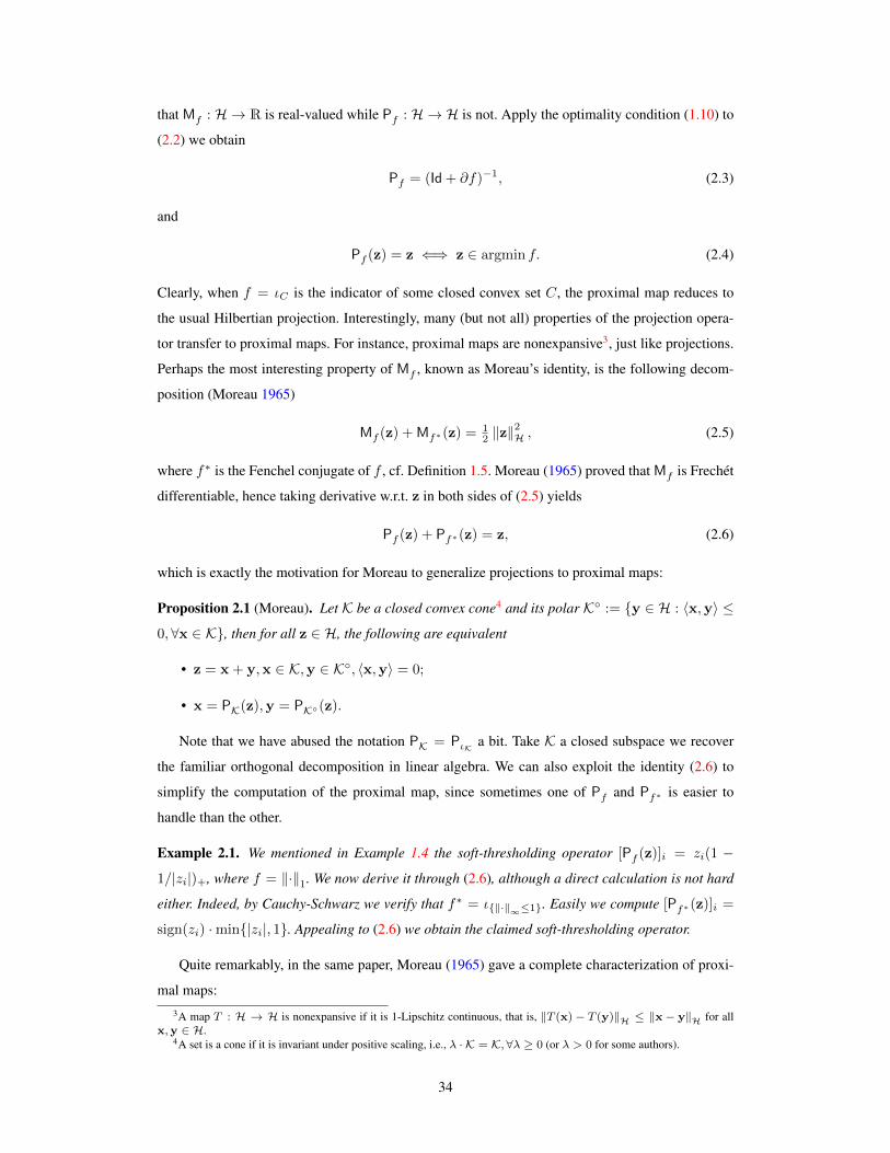
that Mf : H → R is real-valued while Pf : H → H is not. Apply the optimality condition (1.10) to
(2.2) we obtain
Pf = (Id + ∂f)−1, (2.3)
and
Pf (z) = z ⇐⇒ z ∈ argmin f. (2.4)
Clearly, when f = ιC is the indicator of some closed convex set C, the proximal map reduces to
the usual Hilbertian projection. Interestingly, many (but not all) properties of the projection opera-
tor transfer to proximal maps. For instance, proximal maps are nonexpansive3, just like projections.
Perhaps the most interesting property of Mf , known as Moreau’s identity, is the following decom-
position (Moreau 1965)
Mf (z) + Mf∗(z) = 12 ‖z‖
2H , (2.5)
where f∗ is the Fenchel conjugate of f , cf. Definition 1.5. Moreau (1965) proved that Mf is Frechét
differentiable, hence taking derivative w.r.t. z in both sides of (2.5) yields
Pf (z) + Pf∗(z) = z, (2.6)
which is exactly the motivation for Moreau to generalize projections to proximal maps:
Proposition 2.1 (Moreau). Let K be a closed convex cone4 and its polar K := y ∈ H : 〈x,y〉 ≤0,∀x ∈ K, then for all z ∈ H, the following are equivalent
• z = x + y,x ∈ K,y ∈ K, 〈x,y〉 = 0;
• x = PK(z),y = PK(z).
Note that we have abused the notation PK = PιK a bit. Take K a closed subspace we recover
the familiar orthogonal decomposition in linear algebra. We can also exploit the identity (2.6) to
simplify the computation of the proximal map, since sometimes one of Pf and Pf∗ is easier to
handle than the other.
Example 2.1. We mentioned in Example 1.4 the soft-thresholding operator [Pf (z)]i = zi(1 −1/|zi|)+, where f = ‖·‖1. We now derive it through (2.6), although a direct calculation is not hard
either. Indeed, by Cauchy-Schwarz we verify that f∗ = ι‖·‖∞≤1. Easily we compute [Pf∗(z)]i =
sign(zi) ·min|zi|, 1. Appealing to (2.6) we obtain the claimed soft-thresholding operator.
Quite remarkably, in the same paper, Moreau (1965) gave a complete characterization of proxi-
mal maps:3A map T : H → H is nonexpansive if it is 1-Lipschitz continuous, that is, ‖T (x)− T (y)‖H ≤ ‖x− y‖H for all
x,y ∈ H.4A set is a cone if it is invariant under positive scaling, i.e., λ · K = K, ∀λ ≥ 0 (or λ > 0 for some authors).
34

Theorem 2.1 (Moreau (1965)). P : H → H is the proximal map of some function f ∈ Γ0 if and
only if it is nonexpansive and there exists M ∈ Γ0 such that ∀z ∈ H,P(z) ∈ ∂M(z).
The downside though, is that the latter condition, that is, whether or not a given map is the sub-
differential of a closed proper convex function, is hard to verify in general5. Some exceptions are
summarized below.
Corollary 2.1. The linear map A : H → H is a proximal map if and only if it is nonexpansive,
self-adjoint and positive6.
Corollary 2.2. The map P : R → R is a proximal map if and only if it is nonexpansive and
monotonically increasing.
More properties of proximal maps will be presented in Chapter 3, and Proposition 2.4 below.
2.3 Decomposition
Our main goal is to investigate and understand the equality
Pf+g?= Pf Pg
?= Pg Pf , (2.7)
where f, g ∈ Γ0 and f g denotes the mapping composition. Out interest of (2.7) comes from
combining say two regularizers f and g: (2.7) allows us to reduce the computation of Pf+g to a
simple function of Pf and Pg , which themselves can be computed in many cases, as we will see.
Note that Γ0 is not a convex set since the sum of two convex functions in Γ0, sayf and g, could have
empty domain, making the proximal map Pf+g undefined. We exclude this triviality, i.e. f+g ≡ ∞,
in the whole chapter since it is clearly not of our interest.
Under the technical assumption7 ∂(f + g) = ∂f + ∂g, and use (2.3),
Pf+g = (Id + ∂(f + g))−1 = (Id + ∂f + ∂g)−1 =
[(Id + 2∂f) + (Id + 2∂g)
2
]−1
=
[P−1
2f + P−12g
2
]−1
= (P−12f + P−1
2g )−1 (2Id). (2.8)
However, computationally this formula is of little use. On the other hand, it is possible to de-
velop forward-backward splitting procedures to numerically compute Pf+g , using only Pf and
Pg as subroutines (Combettes et al. 2011). In some sense, this procedure is to compute Pf+g ≈limt→∞(Pf Pg)t, modulo some intermediate steps. Our focus is on the exact closed-form formula
(2.7), essentially, establishing the one-step convergence of the iterative procedure of Combettes et al.
5Another equivalent condition that we are aware of is the maximal cyclic monotonicity, which does not appear to be easyto verify either.
6Meaning that 〈z, Az〉 ≥ 0 for all z ∈ H.7Note that the former always contains the latter while the reverse holds when, say one of the functions is continuous at
some point in dom f ∩ dom g, see Ekeland and Témam (1999, Proposition 5.6).
35

x1
x2
f = ιx1=x2
g = ιx2=0
Figure 2.1: Composition of (linear) projections fails to be a proximal map.
(2011). Interestingly, under some “shrinkage” assumption, the prox-decomposition (2.7), even when
it is false, can still be used in subgradient algorithms (Martins et al. 2011).
Our first result is encouraging:
Proposition 2.2. IfH = R, then for any f, g ∈ Γ0, there exists h ∈ Γ0 such that Ph = Pf Pg .
Proof. Since both Pf and Pg are increasing and nonexpansive, it follows easily that so is Pf Pg .
By Corollary 2.2 there exists some h ∈ Γ0 so that Ph = Pf Pg .
In a general Hilbert space H, we again easily conclude that the composition Pf Pg is always
a nonexpansion, which means that it is “close” to be a proximal map. This justifies the composition
Pf Pg as a candidate for the decomposition of Pf+g . However, we note that Proposition 2.2 indeed
can fail already in R2:
Example 2.2. Let H = R2. Let f = ιx1=x2 and g = ιx2=0. Clearly both f and g are in Γ0.
The proximal maps in this case are simply (linear) projections:
Pf =
[0.5 0.50.5 0.5
], Pg =
[1 00 0
].
Therefore
Pf Pg =
[0.5 00.5 0
]is a linear map that is not self-adjoint, hence by Corollary 2.1 it is not a proximal map. It is also clear
that any nontrivial scaling of Pf Pg cannot help either8. See Figure 2.1 for a pictorial illustration.
8In fact, proximal maps are firmly nonexpansive (Bauschke and Combettes 2011). Notice that for sufficiently smallα > 0,α · Pf Pg is firmly nonexpansive. Therefore even firm nonexpansions need not be proximal maps, even inR2.
36

Even worse, when Proposition 2.2 does hold, in general we can not expect the decomposition
(2.7) to be true without additional assumptions.
Example 2.3. Let H = R and q(x) = 12x
2. It is easily seen that Pλq(x) = 11+λx. Therefore
Pq Pq = 14 Id 6= 1
3 Id = Pq+q. We will give an explanation for this failure of composition shortly.
Nevertheless, as we will see, the equality in (2.7) does hold in many scenarios, and an interesting
theory can be suitably developed.
2.3.1 A Sufficient Condition
We start with a sufficient condition that yields (2.7). This result, although easy to obtain, will play a
key role in our subsequent development.
Using the optimality condition (1.10) and the definition of the proximal map (2.2), we have
Pf+g(z)− z + ∂(f + g)(Pf+g(z)) 3 0 (2.9)
Pg(z)− z + ∂g(Pg(z)) 3 0 (2.10)
Pf (Pg(z))− Pg(z) + ∂f(Pf (Pg(z))) 3 0. (2.11)
Adding the last two equations we obtain
Pf (Pg(z))− z + ∂g(Pg(z)) + ∂f(Pf (Pg(z))) 3 0. (2.12)
Comparing (2.9) and (2.12) gives us a simple rule:
Theorem 2.2. A sufficient condition for Pf+g(z) = Pf(Pg(z)
)for all z ∈ H is that
∀ y ∈ dom g, ∂g(Pf (y)) ⊇ ∂g(y). (2.13)
Proof. Let y = Pg(z). Then by (2.12) and the subdifferential rule ∂(f + g) ⊇ ∂f + ∂g we verify
that Pf (Pg(z)) satisfies the optimality condition (2.9), hence follows Pf+g(z) = Pf(Pg(z)
)since
the proximal map is single-valued.
We note that a special form of our sufficient condition has appeared in the proof of Zhou et al.
(2012, Theorem 1), whose main result also follows immediately from our Theorem 2.5 below. Let
us fix f , and define
Kf = g ∈ Γ0 : f + g 6≡ ∞, (f, g) satisfy (2.13). (2.14)
This yields immediately the next result.
Proposition 2.3. For any f ∈ Γ0, Kf is a cone. Moreover, if g1 ∈ Kf , g2 ∈ Kf , f + g1 + g2 6≡ ∞and ∂(g1 + g2) = ∂g1 + ∂g2, then g1 + g2 ∈ Kf too.
37

The last condition ∂(g1 + g2) = ∂g1 + ∂g2 in Proposition 2.3 is purely technical; it is satisfied
when, say one of g1 and g2 is continuous at a single, arbitrary point in dom g1∩dom g2 (Ekeland and
Témam 1999, Proposition 5.6). For comparison purpose, we note that it is not clear how Pf+g+h =
Pf Pg+h would follow from Pf+g = Pf Pg and Pf+h = Pf Ph. This is the main motivation
to consider the sufficient condition (2.13), which also explains the next definition.
Definition 2.1. We call f ∈ Γ0 self-prox-decomposable (s.p.d.) if f ∈ Kαf for all α > 0.
For any s.p.d. f , since Kf is a cone, βf ∈ Kαf for all α, β ≥ 0. Consequently, P(α+β)f = Pβf Pαf = Pαf Pβf .
Remark 2.1. A weaker definition for s.p.d. is to require f ∈ Kf , from which we conclude that
βf ∈ Kf for all β ≥ 0, in particular P(m+n)f = Pnf Pmf = Pmf Pnf for all natural numbers
m and n. The two definitions coincide for positively homogeneous functions. We have not been able
to construct a function that satisfies this weaker definition but not the stronger one in Definition 2.1.
Example 2.4. We easily verify that all affine functions ` = 〈·,a〉 + b are s.p.d., in fact, they are
the only differentiable functions that are s.p.d., which explains why Example 2.3 must fail. Another
trivial class of s.p.d. functions are projectors to closed convex sets. Also, univariate positively homo-
geneous convex functions are s.p.d., due to Theorem 2.5 below. Some multivariate s.p.d. functions
are given in Remark 2.5 below.
The next example shows that the sufficient condition (2.13) is not necessary.
Example 2.5. Fix w ∈ H, f = ιw, and g ∈ Γ0 with full domain. Clearly for any x ∈ H,
Pf+g(z) = w = Pf [Pg(z)]. However, since z is arbitrary, ∂g(Pf (z)) = ∂g(w) 6⊇ ∂g(z) if g is not
linear.
If dim(H) = 1, we can let f = ι[a,b] for some b ≥ a and, say g(x) = 12x
2. Theorem 2.3 below
proves that Pf+g = Pf Pg always holds. Clearly, the sufficient condition (2.13) is necessary only
for points in the interval [a, b].
On the other hand, if f and g are differentiable, then we actually have equality in (2.13), which
is clearly necessary in this case. Since convex functions are almost everywhere differentiable (in the
interior of their domain), we expect the sufficient condition (2.13) to be necessary “almost every-
where” too.
Thus we see that the key for the decomposition (2.7) to hold is to let the proximal map of f and
the subdifferential of g “interact well” in the sense of (2.13). Interestingly, both are fully equivalent
to the function itself9:
Proposition 2.4 (Moreau (1965)). Let f, g ∈ Γ0. The following are equivalent:
9In essence, the equivalence of i) and ii) is the familiar result in calculus. It remains true in an arbitrary Banach space butcould fail in, say, an incomplete inner product space.
38

i). f = g + c for some c ∈ R;
ii). for all w ∈ H, ∂f(w) ⊆ ∂g(w);
iii). Pf = Pg .
Proof. i)⇒ ii): This is clear.
ii) ⇒ iii): From (2.3) Pf = (Id + ∂f)−1, hence Pf ⊆ Pg . But both are single-valued and
everywhere defined, therefore we have in fact equality.
iii)⇒ i): Note that Pf is in fact the derivative of Mf∗ , therefore by integration Pf = Pg implies
that Mf∗ = Mg∗ − c for some c ∈ R. Conjugating we get (Mf∗)∗ = (Mg∗)
∗ + c. But (Mf∗)∗ =
f + 12 ‖·‖
2H. Canceling the squared norm we obtain f = g + c.
Due to the equivalence in Proposition 2.4, some properties of the proximal map will transfer to
corresponding properties of the function f itself, and vice versa. The next result is easy to obtain,
and appeared essentially in Combettes and Pesquet (2007).
Proposition 2.5. Let f ∈ Γ0 and z ∈ H be arbitrary, then
i). Pf is odd if and only if f is even;
ii). Pf (Uz) = UPf (z) for all orthonormal matrices U if and only if f(Uz) = f(z) for all
orthonormal matrices U ;
iii). Pf (Qz) = QPf (z) for all permutation Q (under some fixed basis) if and only if f is permuta-
tion invariant, that is f(Qz) = f(z) for all permutation Q.
Proof. The if parts follow from direct calculation. For the only if part in, say i), we verify directly
from (2.2) that Pf(−·)(z) = −Pf (−z) = Pf (z). Applying Proposition 2.4 we know f is even.
The other two cases are proved similarly.
In the following, we will put some invariance assumptions on the subdifferential of g and ac-
cordingly find the right family of f whose proximal map “respects” that invariance. This way we
will meet (2.13) by construction, hence effortlessly enjoy the prox-decomposition (2.7).
2.3.2 No Invariance
To begin with, consider first the trivial case where no invariance on the subdifferential of g is as-
sumed. This is equivalent as requiring (2.13) to hold for all g ∈ Γ0. Not surprisingly, we end up with
a trivial choice of f .
Theorem 2.3. Fix f ∈ Γ0. Pf+g = Pf Pg for all g ∈ Γ0 if and only if
• dim(H) ≥ 2; f ≡ c, or f = ιw + c for some c ∈ R and w ∈ H;
• dim(H) = 1 and f = ιC + c for some closed and convex set C and c ∈ R.
39

Proof. ⇐: We remind that the implicit constraint f + g 6≡ ∞ is always in force. We need only
consider dim(H) = 1 as the other case is clear. By definition
Pf+g(z) = argminx∈C
hz(x) := 12 (z − x)2 + g(x).
Setting the derivative of hz(x) to zero we obtain x∗ = Pg(z). Crucially, we observe that the one
dimensional convex function hz(x) is decreasing on ] infdom g, x∗[ and increasing on ]x∗,∞[.
Also C = [a, b] is a closed interval. Therefore, if a ≤ x∗ ≤ b, we have Pf+g(z) = x∗; if x∗ ≥ b,
Pf+g(z) = b; and if x∗ ≤ a, Pf+g(z) = a. In all cases, we verify Pf+g(z) = Pf (x∗) = Pf (Pg(z)).
⇒: We first prove that f is constant on its domain even when g is restricted to indicators. Indeed,
let x ∈ dom f and take g = ιx. Then x = Pf+g(x) = Pf [Pg(x)] = Pf (x), meaning that
x ∈ argmin f , cf. (2.4). Since x ∈ dom f is arbitrary, f is constant on its domain. The case
dim(H) = 1 is complete. We consider the other case where dim(H) ≥ 2 and dom f contains at
least two points. If dom f 6= H, there exists z 6∈ dom f such that Pf (z) = y for some y ∈ dom f ,
and closed convex set C∩dom f 6= ∅ with y 6∈ C 3 z. Let g = ιC we obtain Pf+g(z) ∈ C∩dom f
while Pf (Pg(z)) = Pf (z) = y 6∈ C, contradiction.
The fundamental difference between dim(H) = 1 and dim(H) ≥ 2 is not accidental; we will
see it again below. Moreover, we notice that the prox-decomposition (2.7) is not symmetric in f and
g, also reflected in the next result:
Theorem 2.4. Fix g ∈ Γ0. Pf+g = Pf Pg for all f ∈ Γ0 if and only if g is a continuous affine
function.
Proof. ⇐: If g = 〈·,a〉+ c, then Pg(z) = z− a. Easy calculation reveals that Pf+g(z) = Pf (z−a) = Pf [Pg(z)].
⇒: The converse is true even when f is restricted to continuous linear functions. Indeed, let
a ∈ H be arbitrary and consider f = 〈·,a〉. Then Pf+g(z) = Pg(z−a) = Pf (Pg(z)) = Pg(z)−a.
Letting a = z yields Pg(z) = z + Pg(0) = P〈·,−Pg(0)〉(z). Since z is arbitrary, by Proposition 2.4
we know that g is equal to a continuous affine function.
Naturally, the next step is to put invariance assumptions on the subdifferential of g, effectively
restricting the function class of g. As a trade-off, the function class of f , that satisfies (2.13), becomes
larger so that nontrivial results will arise.
2.3.3 Scaling Invariance
The first invariant property we consider is scaling-invariance. What kind of convex functions have
their subdifferential invariant to (positive) scaling, that is ∂g(λ · w) = ∂g(w) for all λ > 0?
40

Assuming 0 ∈ dom g and by simple integration10
g(tz)− g(0) =
∫ t
0
g′(sz)ds =
∫ t
0
〈z, ∂g(sz)〉ds = t · [g(z)− g(0)],
where the last equality follows from the scaling invariance of the subdifferential of g. Therefore, up
to some additive constant, g is positively homogeneous (p.h.). On the other hand, if g ∈ Γ0 is p.h.
(automatically 0 ∈ dom g), then from definition we verify that ∂g is scaling-invariant. Therefore,
under the scaling-invariance assumption, g consists of all p.h. functions in Γ0, up to some addi-
tive constant. Consequently, the requirement on f is to have its proximal map Pf (z) = λz · z for
some λz ∈ [0, 1] that may depend on z as well11. The next theorem completely characterizes such
functions.
Theorem 2.5. Let f ∈ Γ0. Consider the statements
i). f = h(‖·‖H) for some increasing function h : R+ → R ∪ ∞;
ii). For all perpendicular x ⊥ y =⇒ f(x + y) ≥ f(y);
iii). For all z ∈ H, Pf (z) = λz · z for some λz ∈ [0, 1];
iv). 0 ∈ dom f and Pf+κ = Pf Pκ for all p.h. (up to some additive constant) functions κ ∈ Γ0.
Then we have i) =⇒ ii) ⇐⇒ iii) ⇐⇒ iv). Moreover, when dim(H) ≥ 2, ii) =⇒ i) as well, in
which case Pf (z) = Ph(‖z‖H)/ ‖z‖H · z (where we interpret 0/0 = 0).
Remark 2.2. When dim(H) = 1, ii) is equivalent as requiring f to attain its minimum at 0, in which
case the implication ii) =⇒ iv), under the redundant condition that f is differentiable, was proved
by Combettes and Pesquet (2007, Proposition 3.6). The implication ii) =⇒ iii) also generalizes
Combettes and Pesquet (2007, Corollary 2.5), where only the case dim(H) = 1 and f differentiable
was considered. Note that there exists non-even f that satisfies Theorem 2.5 when dim(H) = 1.
Such is impossible for dim(H) ≥ 2, in which case any f that satisfies Theorem 2.5 must also enjoy
all properties listed in Proposition 2.5.
Proof. i) =⇒ ii): For perpendicular vectors x ⊥ y, we have ‖x + y‖H ≥ ‖y‖H.
ii) =⇒ iii): Fix z ∈ H. For x ∈ H, let x = λz + z⊥ be its orthogonal decomposition. By
definition
Mf (z) = minx
12‖x− z‖2 + f(x)
= minz⊥,λ
12‖z⊥ + λz− z‖2 + f(z⊥ + λz)
= minλ
12‖λz− z‖2 + f(λz)
10Here g′(sz), as a function of the scalar s, denotes its right derivative, or, thanks to the convexity of g and the “robustness”of integration, any other sensible selection of the subdifferential.
11Note that λz ≤ 1 is necessary since any proximal map is nonexpansive.
41

= minλ∈[0,1]
12 (λ− 1)2‖z‖2 + f(λz),
where the third equality is due to ii), and the additional constraints on λ in the last equality can
be seen as follows: For any λ < 0, by increasing it to 0 we can only decrease both terms; similar
argument for λ > 1. Therefore there exists λz ∈ [0, 1] such that λzz minimizes the Moreau envelop
Mf hence we have Pf (z) = λzz due to uniqueness.
iii) =⇒ iv): Note first that from iii) we have Pf (0) = 0, implying 0 ∈ ∂f(0) hence 0 ∈ dom f .
Since the subdifferential of κ is scaling-invariant, iii) implies the sufficient condition (2.13) hence
iv).
iv) =⇒ iii): Fix z ∈ dom f and construct the p.h. convex function
κ(x) =
0, if x = λ · z for some λ ≥ 0∞, otherwise .
Then Pκ(z) = z, hence Pf (Pκ(z)) = Pf (z) = Pf+κ(z) by iv). On the other hand,
Mf+κ(z) = minx
12 ‖x− z‖2H + f(x) + κ(x)
= minλ≥0
12 ‖λz− z‖2H + f(λz). (2.15)
Take z = 0 we obtain Pf+κ(0) = 0. Thus Pf (0) = 0, i.e. 0 ∈ ∂f(0), from which we deduce that
Pf (z) = Pf+κ(z) = λz for some λ ∈ [0, 1], since f(λz) in (2.15), as a convex function of λ, is
increasing on [1,∞[.
iii) =⇒ ii): First note that iii) implies that Pf (0) = 0 hence 0 ∈ ∂f(0), in particular, 0 ∈dom f . If dim(H) = 1 we are done, so we assume dim(H) ≥ 2 in the rest of the proof. In this case,
by Theorem 2.7 below we know that ii) is equivalent as i), even without assuming f convex. All we
left is to prove iii) =⇒ ii) or equivalently i), for the case dim(H) ≥ 2.
We first prove the case when dom f = H. By iii), Pf (z) = λzz for some λz ∈ [0, 1]. Using
the optimality condition (1.10) for the proximal map we have 0 ∈ λzz − z + ∂f(λzz), that is
( 1λz− 1)y ∈ ∂f(y) for each y = λzz ∈ Range(Pf ) = H, due to our assumption dom f = H.
Now for any perpendicular vectors x ⊥ y, by the definition of the subdifferential,
f(x + y) ≥ f(y) + 〈x, ∂f(y)〉 = f(y) +⟨x, ( 1
λz− 1)y
⟩= f(y).
Note that when λz = 0, y = 0 and the above inequality still holds.
For the case when dom f ⊂ H, we consider the proximal average (Bauschke et al. 2008; Moreau
1965)
g = A(f, q) = [(12 (f∗ + q)∗ + 1
4q)∗ − q]∗, (2.16)
where q = 12 ‖·‖
2H. The somewhat peculiar formula in the above definition can be derived later when
we discuss the proximal average more thoroughly in Chapter 3. Here, we exploit two nice properties
of the proximal average: Firstly, since q is defined on the whole space, the proximal average g has full
42

0
C
Figure 2.2: Characterization of the “roundness” of the Hilbertian ball.
domain too (Bauschke et al. 2008, Corollary 4.7); Secondly, Pg(z) = 12Pf (z) + 1
4z = ( 12λz + 1
4 )z.
Therefore by our previous argument, g satisfies ii) hence also i). It is easy to check that i) is preserved
under taking the Fenchel conjugation (note that the convexity of f implies that of h). Since we have
shown that g satisfies i), it follows by repeatedly conjugating (2.16) that f satisfies i) hence also ii).
As mentioned, when dim(H) ≥ 2, the implication ii) =⇒ i) will be proven in Theorem 2.7
below. The formula Pf (z) = Ph(‖z‖H)/ ‖u‖H · z for f = h(‖·‖H) follows from straightforward
calculation.
Remark 2.3. The idea behind the proof for iii) =⇒ ii) in Theorem 2.5 seems worth reiterating: The
main difficulty is the subdifferentiability of the function f at points on the boundary of its effective
domain. However, if the property we are interested in, such as being a function of the norm ‖·‖H,
is preserved under taking Fenchel conjugation and is also enjoyed by, say the quadratic function
q = 12 ‖·‖
2H, we can assume without loss of generality that f has full domain, for otherwise we
just consider its proximal average (see (2.16)) with q—a bona fide convex function that is defined
everywhere. This frees us from considering “unfriendly” points, and repeated conjugating can bring
us back to f , without harming the property we are interested in. We expect this simple trick to have
more applications.
We now discuss some applications of Theorem 2.5. When dim(H) ≥ 2, iii) in Theorem 2.5
automatically implies that the scalar constant λz depends on z only through its norm. This fact,
although not entirely obvious, does have a clear geometric picture, as shown in Figure 2.2 and
formalized below.
Corollary 2.3. Let dim(H) ≥ 2, C ⊆ H be a closed convex set that contains the origin. Then the
projection of any point onto C is always a shrinkage towards the origin (i.e., lying somewhere on
the line segment connecting the point and the origin) if and only if C is a ball (of the norm ‖·‖H).
43

−3 −2 −1 0 1 2 3−2
−1
0
1
2
3η = 1
Huber
Berhu
Pη
|·|
Pη
f
Pη
h
Figure 2.3: The proximal map of the Berhu regularizer.
Proof. The slight complication is that different points, even with the same length, may shrink to the
origin with varying degrees. Excluding this possibility is not entirely trivial.
Let f = ιC and apply Theorem 2.5.
Example 2.6. As usual, denote q = 12 ‖·‖
2H. In many applications, in addition to the regularizer κ
(usually a p.h. convex function), one adds the squared l2 regularizer λq for stability, grouping effect,
strong convexity, etc. This incurs no computational cost in the sense of computing the proximal map:
We easily compute that Pλq = 1λ+1 Id. By Theorem 2.5, for any p.h. convex function κ, Pκ+λq =
1λ+1Pκ, whence it is also clear that adding an extra squared l2 regularizer tends to double “shrink”
the solution. In particular, let H = Rd and take κ to be the l1 norm, we recover the proximal map
for the elastic-net regularizer proposed by Zou and Hastie (2005).
Example 2.7. LetH = R. The Berhu regularizer (with parameter γ > 0)
h(x) = |x|1|x|<γ + x2+γ2
2γ 1|x|≥γ = |x|+ (|x|−γ)2
2γ 1|x|≥γ , (2.17)
being the reverse (even in its name!) of Huber’s function (cf. Example 1.4), is proposed in Owen
(2007) as a bridge between the lasso (l1 regularization) and ridge regression (squared l2 regular-
ization). Let f(x) = h(x) − |x|. Clearly, f satisfies ii) of Theorem 2.5 (but not differentiable),
hence
Ph = Pf P|·|,
whereas simple calculation verifies that
Pf (x) = sign(x) ·min|x|, γ1+γ (|x|+ 1),
and of course P|·|(x) = sign(x) ·max|x| − 1, 0. See Figure 2.3 for an illustration. Note that this
regularizer is not s.p.d.
44

Corollary 2.4. Let dim(H) ≥ 2, then the p.h. function f ∈ Γ0 satisfies any item of Theorem 2.5 if
and only if it is a positive multiple of the norm ‖·‖H.
Proof. Theorem 2.8 below showed that under positive homogeneity, i) in Theorem 2.5 implies that
f is a positive multiple of the norm.
Therefore, (positive multiples of) the Hilbertian norm is the only p.h. convex function f that
satisfies Pf+κ = Pf Pκ for all p.h. convex functions κ. In particular, this means that the norm
‖·‖H is s.p.d. (cf. Definition 2.1). Moreover, we easily recover the following result that is perhaps
not so obvious at first glance:
Corollary 2.5 (Jenatton et al. (2011)). Fix the orthonormal basis eii∈I of H. Let G ⊆ 2I be a
collection of tree-structured groups, that is, either g ⊆ g′ or g′ ⊆ g or g ∩ g′ = ∅ for all g, g′ ∈ G.
Then
P∑ni=1 ‖·‖gi = P‖·‖g1 · · · P‖·‖gn ,
where we arrange the groups so that gi ⊂ gj =⇒ i > j, and the notation ‖ · ‖gi denotes the
Hilbertian norm that is restricted to the subspace spanned by the variables in group gi.
Proof. Let f = ‖ · ‖g1 and κ =∑ni=2 ‖ · ‖gi . Clearly they are both p.h. (and convex). By the
tree-structured assumption we can partition κ = κ1 + κ2, where gi ⊂ g1 for all gi appearing in κ1
while gj ∩ g1 = ∅ for all gj appearing in κ2. Restricting to the subspace spanned by the variables
in g1 we can treat f as the Hilbertian norm. Apply Theorem 2.5 we obtain Pf+κ1= Pf Pκ1
.
On the other hand, due to the non-overlapping property, it follows from an easy calculation that
P(f+κ1)+κ2= Pf+κ1
Pκ2, thus a similar reasoning yields
P∑ni=1 ‖·‖gi = P‖·‖g1 P∑n
i=2 ‖·‖gi .
We can clearly iterate the argument to unravel the proximal map as claimed.
For notational clarity, we have chosen not to incorporate weights in the sum of group seminorms:
Such can be absorbed into the seminorm and the corollary clearly remains intact. Our proof also
reveals the fundamental reason why Corollary 2.5 is true: The Hilbertian norm admits the prox-
decomposition (2.7) for any p.h. convex function g! This fact, to the best of our knowledge, has not
been recognized previously.
Note that the tree-structured set system G in Corollary 2.5 is called laminar in combinatorics.
The name “tree-structured” comes from the fact that we can always rearrange the variables to sit
in a rooted tree (or forest more generally) so that the groups in G are simply rooted subtrees, see
Figure 2.4 and Korte and Vygen (2012, Proposition 2.14). Somewhat disappointingly, the number of
groups in a laminar system is at most twice the number of variables (Korte and Vygen 2012, Corol-
lary 2.15), therefore tree-structured groups are not substantially more powerful than non-overlapping
groups (whose size can be the number of variables).
45
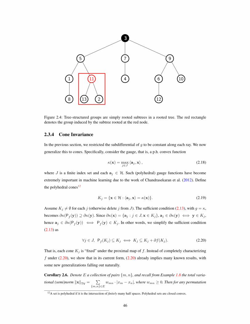
3
5
1
8
11
13 2
7
4
9
6
12
10
Figure 2.4: Tree-structured groups are simply rooted subtrees in a rooted tree. The red rectangledenotes the group induced by the subtree rooted at the red node.
2.3.4 Cone Invariance
In the previous section, we restricted the subdifferential of g to be constant along each ray. We now
generalize this to cones. Specifically, consider the gauge, that is, a p.h. convex function
κ(x) = maxj∈J〈aj ,x〉 , (2.18)
where J is a finite index set and each aj ∈ H. Such (polyhedral) gauge functions have become
extremely important in machine learning due to the work of Chandrasekaran et al. (2012). Define
the polyhedral cones12
Kj = x ∈ H : 〈aj ,x〉 = κ(x). (2.19)
Assume Kj 6= ∅ for each j (otherwise delete j from J). The sufficient condition (2.13), with g = κ,
becomes ∂κ(Pf (y)) ⊇ ∂κ(y). Since ∂κ(x) = aj : j ∈ J,x ∈ Kj, aj ∈ ∂κ(y) ⇐⇒ y ∈ Kj ,
hence aj ∈ ∂κ(Pf (y)) ⇐⇒ Pf (y) ∈ Kj . In other words, we simplify the sufficient condition
(2.13) as
∀j ∈ J, Pf (Kj) ⊆ Kj ⇐⇒ Kj ⊆ Kj + ∂f(Kj). (2.20)
That is, each cone Kj is “fixed” under the proximal map of f . Instead of completely characterizing
f under (2.20), we show that in its current form, (2.20) already implies many known results, with
some new generalizations falling out naturally.
Corollary 2.6. Denote E a collection of pairs m,n, and recall from Example 1.8 the total varia-
tional (semi)norm ‖x‖TV =∑
m,n∈Ewmn · |xm − xn|, where wmn ≥ 0. Then for any permutation
12A set is polyhedral if it is the intersection of finitely many half spaces. Polyhedral sets are closed convex.
46

invariant function13 f , we have
Pf+‖·‖TV = Pf P‖·‖TV .
Proof. Pick an arbitrary pair m,n ∈ E and let κ = |xm−xn|. Clearly J = 1, 2,K1 = xm ≥xn and K2 = xm ≤ xn. Since f is permutation invariant, its proximal map Pf (x) maintains
the relative order of entries in x, see Proposition 2.5, hence we establish (2.20). The other way to
get (2.20) is to verify, simply from the definition, that the subdifferential of a permutation invariant
function is itself permutation invariant. Finally apply Proposition 2.3 and Theorem 2.2.
The special case where f is the l1 norm, appeared first in Friedman et al. (2007), see Example 1.8.
The generalization to any lp norm appeared in Zhang et al. (2013).
We call the permutation invariant function f symmetric if for all x, f(|x|) = f(x), where | · |denotes the componentwise absolute value. The proof for the next corollary is almost the same as that
of Corollary 2.6, except that we also use the simple fact sign([Pf (x)]i) = sign(xi) for symmetric
functions (or the fact that the subdifferential of a symmetric function is itself symmetric).
Corollary 2.7. As in Corollary 2.6, define the (semi)norm
‖x‖oct =∑
m,n∈Ewmn ·max|xm|, |xn|.
Then for any symmetric function f , Pf+‖·‖oct = Pf P‖·‖oct .
Remark 2.4. This norm ‖·‖oct is proposed in Bondell and Reich (2008) for feature grouping, for it
tends to pull xm and xn together for each m,n ∈ E. Surprisingly, Corollary 2.7 appears to be
new. When the underlying graph of E is complete (and for simplicity let w ≡ 1), the proximal map
P‖·‖oct is derived in Zhong and Kwok (2011), which turns out to be another decomposition result.
Indeed, for i ≥ 2, define κi(x) =∑j≤i−1 max|xi|, |xj |. Thus
‖·‖oct =∑i≥2
κi.
Importantly, we observe that κi is symmetric on the first i− 1 coordinates. We claim that
P‖·‖oct = Pκ|I| . . . Pκ2.
The proof is by recursion: Write ‖·‖oct = f + g, where f = κ|I| (recall that |I| is the dimensionality
of x ∈ H). Note that the subdifferential of g depends only on the ordering and sign of the first
|I| − 1 coordinates while the proximal map of f preserves the ordering and sign of the first |I| −1 coordinates (due to symmetry). If we pre-sort x, the individual proximal maps Pκi(x) become
easy to compute sequentially and we recover the algorithm in Zhong and Kwok (2011) after some
bookkeeping.
13Recall from Proposition 2.5 that f is permutation invariant if for all permutation matrix P we have f(Px) = f(x) forall x. Note that all we need is the weaker condition: For all m,n ∈ E, xm ≥ xn =⇒ [Pf (x)]m ≥ [Pf (x)]n.
47

Corollary 2.8. As in Corollary 2.5, let G ⊆ 2I be a collection of tree-structured groups, then
P∑ni=1‖·‖gi,k
= P‖·‖g1,k · · · P‖·‖gn,k ,
where we arrange the groups so that gi ⊂ gj =⇒ i > j, and ‖x‖gi,k =∑kj=1 |xgi |[j] is the sum
of the k (absolute-value) largest elements in the group gi, i.e., Ky-Fan’s k-norm.
Proof. Similar as in the proof of Corollary 2.5, we need only prove that
P‖·‖g1,k+‖·‖g2,k= P‖·‖g1,k
P‖·‖g2,k ,
where w.l.o.g. we assume g1 contains all variables while g2 ⊂ g1. Therefore ‖·‖g1,k can be treated
as symmetric. To be explicit, let group g2 = i1, . . . , is. Ky-Fan’s k-norm on g2 induces m =(sk
),
or m = 1 if s < k, polyhedral cones Kj , j = 1, . . . ,m. Since f = ‖·‖g1,k is symmetric, Pf (y)
maintains the relative order of magnitudes in y. In other words, Pf (Kj) ⊆ Kj , establishing (2.20).
Applying Theorem 2.2 completes the proof.
Note that the case k ∈ 1, |I|was proved in Jenatton et al. (2011) and Corollary 2.8 can be seen
as an interpolation. Interestingly, there is another interpolated result whose proof should be apparent
now.
Corollary 2.9. Corollary 2.8 remains true if we replace Ky-Fan’s k-norm with
‖x‖oct,k =∑
1≤i1<i2<...<ik≤|I|max|xi1 |, . . . , |xik |. (2.21)
Therefore we can employ the norm ‖x‖oct,2 for feature grouping in a hierarchical manner.
Clearly we can also combine Corollary 2.8 and Corollary 2.9. Our last result does not bring any
new technique but leads to important algorithmic consequences.
Corollary 2.10. For any symmetric f , Pf+‖·‖oct,k = Pf P‖·‖oct,k . Similarly, for Ky-Fan’s k-norm
‖x‖k =∑ki=1 |x|[i], we have Pf+‖·‖k = Pf P‖·‖k .
Remark 2.5. Immediately, Corollary 2.10 implies that Ky-Fan’s k-norm and the norm ‖ · ‖oct,k de-
fined in (2.21) are both s.p.d. (see Definition 2.1). The special case for the lp norm with p ∈ 1, 2,∞was proved in Duchi and Singer (2009, Proposition 11), with a substantially more complicated ar-
gument. As pointed out in Duchi and Singer (2009), s.p.d. regularizers allow us to perform lazy
updates in PG (cf. Section 1.3) or PSG (cf. Section 1.4). Indeed, suppose during the iterate that
the (sub)gradient of the loss ` is sparse, we need to perform the update w.r.t. the regularizer f by
w← Pηtf (w). For those coordinates with (constantly) null (sub)gradient, instead of performing the
proximal map in each step, we could just aggregate them in one-shot: w ← P∑t ηt
f (w), provided
that f is s.p.d. Notice that the lp norm for other p is not s.p.d., as can be quickly verified by numerical
examples, or see Jenatton et al. (2011) for a proof.
48

Of course, we have not exhausted the possibility to have the prox-decomposition (2.7). For in-
stance, all of our results extend to matrix variables, provided that we consider only unitarily invariant
matrix norms, see Appendix A or Yu and Schuurmans (2011) for some relevant discussions. In our
development (and the existing results we are aware of), we heavily build upon the “round” l2 norm
or polyhedral functions14. Whether or not this is a sheer coincidence requires some further work on
understanding the prox-decomposition (2.7).
2.4 Connection with the Representer Theorem
The main goal in this section is to supply the missing piece in the proof of Theorem 2.5, and draw
the connection to the representer theorem in kernel methods. Some background first.
Many kernel methods can be formulated as the optimization problem
infw∈H
`n(〈w,w1〉 , . . . , 〈w,wn〉) + f(w), (2.22)
where `n : Rn → R ∪ ∞ is some loss function, wi ∈ H, i = 1, . . . , n is our data, and
f : H → R ∪ ∞ is the regularizer. Unfortunately, H is usually an infinite dimensional Hilbert
space, thus optimizing (2.22) directly might run into practical issues. However, if we are assured,
by a proper design of the regularizer f , that some minimizer actually lies in the span of the data,
that is w =∑ni=1 αiwi for αi ∈ R, i = 1, . . . , n, we can turn (2.22) into a finite dimensional
problem which simply finds α ∈ Rn. Of course, we need to be able to compute the Gram matrix
Kij = 〈wi,wj〉. Such is the case whenH is the reproducing kernel Hilbert space induced by some
kernel function that is explicitly evaluable, see Aronszajn (1950) for details. Any regularizer f that
enables the outlined reduction is said to satisfy the representer theorem. As a simple consequence of
orthogonal decompositions in Hilbert space, any increasing function of the norm ‖·‖H, in particular
‖·‖2H, satisfies the representer theorem (Kimeldorf and Wahba 1971; Scholköpf and Smola 2001).
The quest is to supply a necessary condition hence completely characterize such regularizers.
As pointed out in Argyriou et al. (2009), to study the representer theorem, one can (and perhaps
should) focus on the interpolation problem:
infw∈H
f(w) s.t. 〈w,wi〉 = yi, i = 1, . . . , n, (2.23)
where y ∈ Rn is given. The advantage of considering interpolation is that the loss function `n
no longer plays any role in the specification. Moreover, it is easy to argue that if f satisfies the
representer theorem in (2.23), it remains so in (2.22) for any loss `n. The converse is also true, under
minor regularity conditions on the loss `n, see Argyriou et al. (2009) and Dinuzzo and Schölkopf
(2012).
To facilitate the discussion, following Argyriou et al. (2009), we define the term admissibility as
follows:14A (convex) function f is polyhedral iff its epigraph (x, t) ∈ H×R : f(x) ≤ t is a polyhedral set.
49

Definition 2.2. The function f : H → R ∪ ∞ is admissible if for all n, (wi ∈ H)ni=1 and
(yi ∈ R)ni=1, some minimizer of (2.23) admits the form
w =
n∑i=1
αiwi (2.24)
for some α ∈ Rn. We consider the statement vacuously true if (2.23) has no minimizer.
The key step towards characterizing admissible functions is due to Argyriou et al. (2009):
Proposition 2.6. LetH be an inner product space. The function f : H → R∪ ∞ is admissible if
and only if
∀x,y ∈ H, 〈x,y〉 = 0 ⇒ f(x + y) ≥ f(x). (2.25)
Proof. ⇒: Suppose f is admissible. Consider the following instance of (2.23):
infw∈H
f(w) s.t. 〈w,x〉 = ‖x‖2H . (2.26)
The admissibility of f implies that x is a minimizer of (2.26). Since x+y, for any y ⊥ x, is feasible
for (2.26), we have f(x + y) ≥ f(x) from the optimality of x.
⇐: Suppose (2.25) holds and (2.23) has a minimizer z = w + w⊥, where w ∈ Hn :=
spanw1, . . . ,wn and w⊥ is in the orthogonal complement ofHn.15 Clearly 〈z,wi〉 = 〈w,wi〉 =
yi, hence w is feasible. Invoking (2.25) we know f(z) ≥ f(w), therefore w is also a minimizer,
proving the admissibility of f .
Although Proposition 2.6 gives a complete characterization of admissibility, the verification of
its conditions can be cumbersome. Argyriou et al. (2009) further proved that for differentiable f , it
is admissible if and only if it is an increasing of the norm ‖·‖H. Dinuzzo and Schölkopf (2012) man-
aged to weaken the differentiability assumption to lower semicontinuity (l.s.c.)16. We now demon-
strate that a modification of their proof removes even the l.s.c. requirement hence yields a complete
characterization of admissibility.
We first make an easy observation. If the vector space H has unit dimension, i.e. dim(H) = 1,
then the condition (2.25) is equivalent as requiring f(w) ≥ f(0) for all w ∈ H. Therefore, for the
remainder of this section we will exclude this trivial case and assume dim(H) ≥ 2 henceforth.
The main result in this section, which, in retrospect could be considered to be the “correct form”
of the representer theorem, is the following:
Theorem 2.6. Let H be an inner product space with dim(H) ≥ 2. A function f : H → R ∪ ∞is admissible if and only if
∀x,y ∈ H, ‖y‖H > ‖x‖H ⇒ f(y) ≥ f(x). (2.27)
15 The existence of such a decomposition depends only on the completeness of Hn, not on that of H. Note that Hn isindeed complete since it is of finite dimension.
16Recall that f : H → R ∪ ∞ is lower semicontinuous iff its sublevel set w ∈ H : f(w) ≤ α is closed for allα ∈ R.
50

θ
6 (x,y)
x0 = x
x1
x2
yxn = py
Ry
yθ
pθqθ
y
s(θ) · y t(θ) · yθ
Figure 2.5: Illustration of the main idea presented in the proof of Theorem 2.6.
Note that we do not require any assumption, such as l.s.c., on f , and (2.27) is not the usual
“increasing” property, but instead a weaker requirement—we henceforth refer to it as the weakly in-
creasing property. Then, the condition equivalent to admissibility can be stated concisely as weakly
increasing w.r.t. the norm ‖·‖H.
Proof. ⇐: Suppose (2.27) holds. We verify (2.25), from which the admissibility of f will follow.
Pick any x,y ∈ H such that 〈x,y〉 = 0,x 6= 0. Then we have ‖x + y‖H > ‖y‖H and thus
by (2.27), f(x + y) ≥ f(y). Noting that the case x = 0 also trivially holds, we see that (2.25)
holds. By Proposition 2.6, we get that f is admissible.
⇒: Suppose now that f is admissible. Then, by Proposition 2.6, (2.25) holds. Note that in the
special case when x = 0 and y 6= 0 (so that ‖y‖H > 0), we have f(y) = f(0+y) ≥ f(0) = f(x).
Therefore, in what follows we need only deal with the case when x 6= 0. To prove (2.27), we start
with a claim.
Claim: The admissibility of f implies f(·) is increasing along any ray Ry = t · y : t ≥ 0,where 0 6= y ∈ H.
By the above reasoning it suffices to prove this claim for Ry \ 0. We prove the claim using
a geometric argument depicted in the left panel of Figure 2.5. For a fixed vector y ∈ H and an
angle θ ∈ [0, π/2[, choose some x ∈ H such that x is not parallel to y. Such an x exists since
dim(H) ≥ 2. Now, let yθ be the rotation of y in the plane (subspace) P spanned by x and y. The
direction of rotation can be chosen arbitrarily. Take the line in the plane P that passes through yθ
and which is orthogonal to yθ. Let t(θ) · y be the point where the ray Ry and the line intersect and
let the vector pθ be defined as yθ + pθ = t(θ) · y. Note that t(θ) = (1 + tan2(θ))1/2 ≥ 1 for all
θ ∈ [0, π/2[. Thus, pθ is orthogonal to yθ: pθ ⊥ yθ. Further, let s(θ)·y be the orthogonal projection
of yθ to the ray Ry and call qθ the vector that satisfies s(θ) · y + qθ = yθ. Thus, qθ ⊥ s(θ) · y.
51

Further, s(θ) = cos(θ) ≤ 1 for all θ ∈ [0, π/2[. Applying (2.25) from Proposition 2.6 twice we get
f(t(θ) · y) = f(yθ + pθ) ≥ f(yθ)
= f(s(θ) · y + qθ) ≥ f(s(θ) · y).(2.28)
Note that this holds for any 0 6= y ∈ H and θ ∈ [0, π/2[.
Now, take any 0 < τ1 < τ2. Since t(θ)/s(θ) is continuous on [0, π/2[ and its range is [1,∞[,
there exists a value θ′ ∈ [0, π/2[ such that
t(θ′)s(θ′)
=τ2τ1
. (2.29)
Define c = τ2/t(θ′). So we also have that c = τ1/s(θ
′) thanks to (2.29). Hence, applying (2.28) to
cy and θ′, we get
f(τ2y) = f(t(θ′) · (cy)
)≥ f
(s(θ′) · (cy)
)= f(τ1y) ,
finishing the proof of the claim.
Now if ‖y‖H > ‖x‖H and x is not aligned with y, it is not hard to see (cf. Figure 2.5, right
panel) that one can find a sufficiently large n ≥ 1, a real number p ∈]0, 1[ and a sequence x0 =
x,x1, . . . ,xn = py such that for any 0 ≤ i ≤ n − 1, the angle ∠(xi,xi+1) = θ := ∠(x,y)/n
and (xi+1 − xi) ⊥ xi. Indeed, n defines the above sequence uniquely with some p = pn > 0.
In particular, pn ‖y‖H = ‖xn‖H = [t(θ/n)]n ‖x‖H, so pn = [t(θ/n)]n‖x‖H‖y‖H
. Since [t(θ/n)]n ∼(1 + (θ/n)2)n
2/θ2·θ2/n ∼ eθ2/n → 1 as n → ∞, pn → ‖x‖H
‖y‖H< 1 and so the existence of (n, p)
with the said properties is guaranteed. Therefore, using the claim and (2.25), we get
f(y) ≥ f(py)
= f(xn) = f(xn−1 + (xn − xn−1))
≥ f(xn−1) = f(xn−2 + (xn−1 − xn−2))
...
≥ f(x0) = f(x) ,
thus finishing the proof of (2.27).
The reason why the continuity conditions can be avoided in Theorem 2.6, making the result
simpler and more elegant, is that the necessary condition for the admissibility of f avoids stipulating
f ’s behavior on the surface of balls. In fact, if one modified (2.27) to include the case when ‖x‖H =
‖y‖H, it would imply that f is radial, i.e., f(x) depends on the argument x only through ‖x‖H. The
next example demonstrates that one can have an admissible regularizer that is not radial (of course,
such an f cannot be semicontinuous).
Example 2.8. Figure 2.6 shows an admissible function f that is not radial. The gray area denotes,
say, the unit ball w ∈ H : ‖w‖H ≤ 1 and the red point represents some y on the unit sphere
52

f(w) = 0
f(w) =∞
f(y) = 1
Figure 2.6: An admissible function f that is not increasing w.r.t. the norm.
w ∈ H : ‖w‖H = 1. It is clear that f is neither l.s.c. nor upper semicontinuous17. Note also
that f is in fact a convex admissible function, demonstrating that convex functions can be “ugly” on
boundary points.
Remark 2.6. As the previous example demonstrates, there exist non-radial, but admissible func-
tions. However, Theorem 2.6 also implies that every admissible function is equal to an admissible
radial function except for a set whose cardinality is at most “countable”. To see this consider the
function I(r) := inff(x) : ‖x‖H = r. Clearly I : R+ → R ∪ ∞ is an increasing function,
hence it can have at most countably many discontinuity points. But it is easily seen that for any
continuity point r of I and any x,y ∈ H on the H-sphere of radius r, it follows that f(x) = f(y).
Thus, f is radial except for at most countably many spheres.
Before refining Theorem 2.6, let us mention that a function f : H → R∪∞ is u.s.c. iff for all
x ∈ H and the sequence xn → x, f(x) ≥ lim supxn→x
f(xn); similar result holds for l.s.c. functions,
with lim sup replaced by lim inf and ≥ replaced by ≤. Of course, f is continuous iff it is both l.s.c.
and u.s.c.
Remark 2.7. One should not confuse the l.s.c. (u.s.c.) of f : H → R ∪ ∞ with the l.s.c. (u.s.c.)
of f : dom f → R. The former condition, used throughout this thesis, is strictly stronger than the
latter condition. For instance, the f in Figure 2.6 is u.s.c. in the latter sense but not u.s.c. in our
standard.
We are now ready to provide the missing piece in the proof of Theorem 2.5. Obviously, any item17Similarly, f is upper semicontinuous (u.s.c.) if its superlevel set w ∈ H : f(w) ≥ α is closed for all α ∈ R.
53

in Theorem 2.5 also gives a different characterization of the representer theorem (under the l.s.c.
assumption).
Theorem 2.7. Let H be an inner product space with dim(H) ≥ 2 and f : H → R ∪ ∞ be u.s.c
or l.s.c., then f is admissible if and only if
∀x,y ∈ H, ‖y‖H ≥ ‖x‖H ⇒ f(y) ≥ f(x), (2.30)
or, in other words, f is an increasing radial function.
Proof. ⇐: (2.30) apparently implies (2.27) hence the admissibility of f .
⇒: Assume that f is u.s.c. and admissible. Thanks to Theorem 2.6, we need only prove that if
‖y‖H = ‖x‖H then f(y) ≥ f(x). To see this, take a sequence yn that converges to y and that
satisfies ‖yn‖H > ‖y‖H. Then, ‖yn‖H > ‖y‖H = ‖x‖H also holds; therefore, by Theorem 2.6,
f(yn) ≥ f(x) holds for all n. Taking the lim sup of both sides, we get f(y) ≥ lim supn→∞
f(yn) ≥f(x).
The l.s.c. case can be proved using an entirely analogous argument, which is essentially the main
result of Dinuzzo and Schölkopf (2012). Note that we cannot naively negate an l.s.c. function here
to reduce to the u.s.c. case, since our starting tool (2.25) is not invariant to negation.
Remark 2.8. Another easy way to see the result in Theorem 2.7 is to notice that the function I(r)
defined in Remark 2.6 is in fact continuous when f satisfies (2.30) (or equivalently (2.25)) and is
either l.s.c. or u.s.c. Based on Theorem 2.6 and Theorem 2.7, it can also be shown that the lower or
upper semicontinuous hulls18 of admissible functions remain so, although the reverse implication is
false.
It turns out that positive homogeneity, other than semicontinuity, also forces admissible func-
tions to be radial. Notice that both properties imply that the function I(r) defined in Remark 2.6 is
continuous.
Theorem 2.8. LetH be an inner product space with dim(H) ≥ 2. If f is admissible and positively
homogeneous, then it is a positive multiple of the induced norm ‖·‖H.
Proof. We prove first that f must be an increasing function of the norm. Note that due to positive
homogeneity, we have f(0) = 0 hence f ≥ 0 by the admissibility. Suppose to the contrary there
exist x,y ∈ H such that ‖x‖H = ‖y‖H 6= 0 but f(x) > f(y). Clearly f(y) < ∞. Then for all
1 < λ < f(x)/f(y), ‖λy‖H = λ ‖y‖H > ‖x‖H, hence f(λy) ≥ f(x) by the admissibility. If
f(y) = 0 then due to positive homogeneity 0 ≥ f(x), contradiction; similarly, if f(y) > 0, due
to again positive homogeneity, λ ≥ f(x)/f(y), contradiction again. Thus f is an increasing radial
function.18The lower semicontinuous hull of a function f is defined as flsc(x) = sup
g≤fg(x), subject to g is continuous. The upper
semicontinuous hull is defined analogously.
54

f(w) = 0
f(w) = 2
f(w) = 1
Figure 2.7: A function f that is increasing radial but not l.s.c. or u.s.c.
Take an arbitrary x0 ∈ dom f with unit norm (i.e., ‖x0‖H = 1), then due to positive homogene-
ity f(x) = ‖x‖H · f(x0). The proof is now complete.
The consequence of Theorem 2.8 is immediate: Essentially, any other (semi)norm defined onH(which may or may not be compatible with the topology of H) can not be admissible. Obviously if
f is admissible and positively homogeneous with degree d > 0 (i.e., f(λx) = λd · f(x)) then we
have f(x) = ‖x‖dH · f(x0) for some (arbitrary) x0 ∈ dom f with unit norm.
The next example shows that neither l.s.c. nor u.s.c. is necessary for f to be an increasing radial
function, i.e. satisfying (2.30).
Example 2.9. Figure 2.7 shows a function that is increasing radial, but is neither l.s.c. nor u.s.c.
Here, the gray region denotes, say the open unit ball w ∈ H : ‖w‖H < 1, while the red circle
represents the unit sphere w ∈ H : ‖w‖H = 1. This example, despite of its triviality, motivates
our next development: We can write
f = [1 · 1‖w‖≤1 + 2 · 1‖w‖>1] ∧ [0 · 1‖w‖<1 + 2 · 1‖w‖≥1],
where ∧ denotes the pointwise infimum and 1C denotes the 0, 1-valued indicator function of the
set C. Observe that the first function is l.s.c. while the second is u.s.c.
Needless to say that, if fγ satisfies (2.27) or (2.30), then so do∑γ fγ , infγ fγ and supγ fγ
respectively (whenever they are well-defined). In fact, the converse is also sort of true, giving us a
necessary and sufficient characterization of (2.30).
55

Theorem 2.9. f satisfies (2.30) if and only if f = f1∧ f2, or f = f1∨ f2, or f = f1 + f2, for some
f1 that is l.s.c. and admissible and some f2 that is u.s.c. and admissible.
Proof. ⇒: Suppose f satisfies (2.30), then there exists an increasing function h : R+ → R ∪ ∞so that f(w) = h(‖w‖H). Obviously h has at most countably many discontinuous points, which
we denote as D := tii∈N (arranged according to their magnitude).
Let us first consider the case f = f1 ∧ f2. If D = ∅, then simply take fi(w) = h(‖w‖H), i =
1, 2; otherwise define19
h1(t) :=∑i∈N
[h(t) + h(ti)− h(ti−)] · 1ti−1<t<ti + h(ti) · 1t=ti ,
which is l.s.c. and increasing. Next define (the so-called u.s.c. hull)20
h2(t) := sups : t ∈ clx : h(x) ≥ s.
It is easily verified that h2 is the smallest u.s.c. function that majorizes h. In our case this amounts
to simply modifying h at the discontinuous points D so that it becomes right continuous. Clearly
h2 is non-decreasing (since h is so). Finally put fi(w) = hi(‖w‖H) and then Theorem 2.9 can be
verified without difficulty.
The case f = f1 ∨ f2 is proved similarly.
For the last case when f = f1 + f2, define
h1(t) :=∑i∈N
[h(t)−
i∑j=1
(h(tj+)− h(tj))]· 1ti<t≤ti+1 + h(t) · 1t≤t1 ,
h2(t) :=∑i∈N
[h(ti+)− h(ti)] · 1ti<t.
One can easily verify that h1 is increasing and u.s.c. while h2 is increasing and l.s.c. Unsurprisingly,
putting fi(w) = hi(‖w‖H) completes the construction.
⇐: Immediate consequence of the remark made before the theorem.
Yu et al. (2013) also extended the results in this section to the matrix setting, although the char-
acterization there is less complete.
2.5 Summary
Motivated by some existing results which all suggest the possibility to decompose the proximal map
of a sum of functions into the composition of the proximal maps of the individual summands, we
first give a positive answer in the one dimensional space and a negative example in general. Then,
we identify a simple sufficient condition that, if satisfied, will imply the desired decomposition.
19In the case D = t1, . . . , tn, we add t0 = 0 and tn+1 =∞ to the set D, in order to handle the boundary.20cl means taking the topological closure of the set.
56

Furthermore, we completely characterize the function class that decomposes with respect to all pos-
itively homogeneous functions; it simply consists of all increasing radial functions. An unexpected
connection to the characterization of the representer theorem in kernel methods is exposed. Finally,
we generalize the prox-decomposition rule to polyhedral functions, under the cone invariance as-
sumption. We recover most known decomposition results, with some new ones obtained almost
effortlessly from our theory.
57

Chapter 3
Proximal Average Approximation
In Chapter 2 we discussed a particular decomposition rule for computing the proximal map of a
sum of functions. Unfortunately, this rule does not always apply. In this chapter we introduce a gen-
eral recipe that is based on the golden principle: We approximate “complicated” functions with more
“friendly” ones. Traditionally, the nonsmooth regularizers are usually approximated by smooth func-
tions. We re-examine this powerful methodology and point out a nonsmooth approximation which
simply pretends the linearity of the proximal map. The new approximation is justified using a recent
convex analysis tool—proximal average, and yields a different proximal gradient algorithm that is
strictly better than the one based on smoothing, without incurring any extra overhead. Numerical
experiments conducted on two important applications, overlapping group LASSO (cf. Example 1.7)
and graph-guided fused LASSO (cf. Example 1.9), corroborate the theoretical claims.
The results in this chapter appeared in Yu (2013a).
3.1 Introduction
In many scientific areas, an important methodology that has withstood the test of time is the ap-
proximation of “complicated” functions by those that are easier to handle. For instance, Taylor’s
expansion in calculus (Rudin 1976), essentially a polynomial approximation of differentiable func-
tions, has fundamentally changed analysis, and mathematics more broadly. Approximations are also
ubiquitous in optimization algorithms, e.g. various gradient-type algorithms approximate the objec-
tive function with a quadratic upper bound. In some (if not all) cases, there are multiple ways to
make the approximation, and one usually has this freedom of choice. It is perhaps not hard to con-
vince oneself that there is no approximation that would work best in all scenarios. And one would
probably also agree that a specific form of approximation should be favored if it well suits our ulti-
mate goal. Despite of all these common-sense, in optimization algorithms, smooth approximations
are still dominating, bypassing some recent advances on optimizing nonsmooth functions, see e.g.
the last three algorithms we reviewed in Chapter 1. Part of the reason, we believe, is the lack of new
technical tools.
58

We consider the composite minimization problem (1.1) where the objective consists of a smooth
loss function and a sum of nonsmooth functions. Such problems have received increasing attention
due to the arise of structured sparsity (Bach et al. 2012), notably the overlapping group LASSO
(Zhao et al. 2009), the graph-guided fused LASSO (Hoefling 2010; Kim and Xing 2009) and some
others. These structured regularizers, although greatly enhance our modeling capability, introduce
significant new computational challenges as well. Popular gradient-type algorithms dealing with
such composite problems include the generic subgradient method (Shor 1985), (accelerated) proxi-
mal gradient (APG) (Beck and Teboulle 2009a; Nesterov 2013), and the smoothed accelerated prox-
imal gradient (S-APG) of Nesterov (2005). The subgradient method is applicable to any nonsmooth
function, although the convergence rate is rather slow. APG, being a recent advance, can handle
simple functions, see e.g. Combettes and Pesquet (2011), Bach et al. (2011, §3.3), Parikh and Boyd
(2013, §6), but for more complicated structured regularizers, an inner iterative procedure is needed,
resulting in an overall convergence rate that could be as slow as the subgradient method (Villa et
al. 2013). Lastly, S-APG simply runs APG on a smooth approximation of the original objective,
resulting in a much improved convergence rate.
Our work is inspired by the recent advance on nonsmooth optimization, such as Beck and
Teboulle (2009a), Duchi et al. (2010), Nesterov (2013), and Xiao (2010), of which the building
block is the proximal map of the nonsmooth function. This proximal map is available in closed-
form for simple functions but can be quite expensive for more complicated functions such as a sum
of nonsmooth functions we consider here. A key observation we make is that oftentimes the prox-
imal map for each individual summand can be easily computed, therefore a bold idea is to simply
use the sum of proximal maps, pretending that the proximal map is a linear operator. Somewhat
surprisingly, this naive idea, when combined with APG, results in a new proximal algorithm that is
strictly better than S-APG, while keeping per-step complexity unchanged. We justify our method via
a new tool from convex analysis—the proximal average (Bauschke et al. 2008). In essence, instead
of smoothing the nonsmooth function, we use a nonsmooth approximation whose proximal map is
cheap to evaluate, after all this is all we need to run APG.
We formally state our problem in Section 3.2, along with the proposed algorithm. After recalling
the relevant tools from convex analysis in Section 3.3 we provide the theoretical justification of our
method in Section 3.4. Related works are discussed in Section 3.5 and refinements are presented in
Section 3.6. We test the proposed algorithm in Section 3.7 and conclude in Section 3.8.
3.2 Problem Formulation
We are interested in solving the following composite minimization problem:
infw∈H
`(w) + f(w), where f(w) =
K∑k=1
αkfk(w). (3.1)
59

Here ` is convex with L-Lipschitz continuous gradient1 w.r.t. the Hilbertian norm ‖·‖H, and αk ≥0,∑k αk = 1. The usual regularization constant that balances the two terms in (3.1) is absorbed
into the loss `. For the functions fk, we make the following assumption.
Assumption 3.1. Each fk is convex and Mk-Lipschitz continuous w.r.t. the Hilbertian norm ‖·‖H.
The abbreviation M2 =∑Kk=1 αkM
2k is adopted throughout.
We are interested in the general case where the functions fk need not be differentiable. As
mentioned in the introduction, a generic scheme that solves (3.1) is the subgradient method (Shor
1985), of which each step requires merely an arbitrary subgradient of the objective. With a suitable
step size, the subgradient method converges2 in at most O(1/ε2) steps where ε > 0 is the desired
accuracy, see Section 1.2 for details. Although being general, the subgradient method is exceedingly
slow, making it unsuitable for many practical applications.
Another recent algorithm for solving (3.1) is the (accelerated) proximal gradient (APG) (Beck
and Teboulle 2009a; Combettes and Wajs 2005; Nesterov 2013), of which each iteration needs to
compute the proximal map of the nonsmooth part f in (3.1):
P1/L
f(w) = argmin
z
L2 ‖w − z‖2 + f(z).
Recall that L is the Lipschitz constant of the gradient of the smooth part ` in (3.1). Provided that the
proximal map can be computed easily, it can be shown that APG converges within O(1/√ε) steps,
significantly better than the subgradient method, see Section 1.3 for details. For some simple func-
tions, the proximal map indeed is available in closed-form, see Combettes and Pesquet (2011), Bach
et al. (2011, §3.3), Parikh and Boyd (2013, §6) for nice summaries. However, for more complicated
functions such as the one we consider here, the proximal map itself is expensive to compute and
an inner iterative subroutine is required. Somewhat disappointingly, recent analysis has shown that
such a two-loop procedure can be as slow as the subgradient method (Villa et al. 2013).
Yet another approach, popularized by Nesterov (2005), is to approximate each nonsmooth com-
ponent fk with a smooth function and then run APG. By carefully balancing the approximation and
the convergence requirement of APG, the smoothed accelerated proximal gradient (S-APG) pro-
posed by Nesterov (2005) converges in at most O(√
1/ε2 + 1/ε) steps, again much better than the
subgradient method. However, the downside is that smoothing always increases the Lipschitz con-
stant. The main point of this chapter is to further improve S-APG, in perhaps a surprisingly simple
way.
The key assumption that we will exploit is the following:
Assumption 3.2. Each proximal map Pηfk can be computed easily for any η > 0.
1Namely ‖∇`(x)−∇`(y)‖H ≤ L · ‖x− y‖H for all x,y ∈ H.2We satisfy ourselves with convergence in terms of function values, although with additional assumptions/efforts it is
possible to argue for convergence in terms of the iterates.
60

Algorithm 5 PA-APG.
1: Initialize w0 = u1, η = min1/L, 2ε/M2, γ1 = 1.2: for t = 1, 2, . . . do3: zt = ut − η∇`(ut),4: wt =
∑k αk · P
ηfk
(zt),
5: γt+1 =1+√
1+4γ2t
2 ,6: ut+1 = wt + γt−1
γt+1(wt −wt−1).
7: end for
Algorithm 6 PA-PG.
1: Initialize w0, η = min1/L, 2ε/M2.2: for t = 1, 2, . . . do3: zt = wt−1 − η∇`(wt−1),4: wt =
∑k αk · P
ηfk
(zt).5: end for
We prefer to leave the exact meaning of “easily” unspecified, but roughly speaking, the proximal
map should be no more expensive than computing the gradient of the smooth part ` so that it does not
become the bottleneck. Both Assumption 3.1 and Assumption 3.2 are satisfied in many important
applications (examples will follow). As it will also become clear later, these assumptions are exactly
those needed by S-APG.
Unfortunately, in general, there is no known efficient way that reduces the proximal map of the
average f to the proximal maps of its individual components fk, therefore the fast schemes PG
or APG are not readily applicable. The main difficulty, of course, is due to the nonlinearity of the
proximal map Pηf , when treated as a map on the function f . Despite of this fact, we will “naively”
pretend that the proximal map is linear and use3
Pηf
?≈K∑k=1
αkPηfk. (3.2)
Under this approximation, the fast schemes PG or APG can be applied. We give one particular
realization (PA-APG) in Algorithm 5 based on the FISTA of Beck and Teboulle (2009a). A simpler,
though slower, version (PA-PG) based on the ISTA of Beck and Teboulle (2009a) is also provided in
Algorithm 6. Clearly both algorithms are easily parallelizable ifK is large. We remark that any other
variant of APG or PG, e.g. Nesterov (2005), is equally well applicable. Of course, when K = 1, our
algorithm reduces to the corresponding APG or PG scheme.
At this point, one might be suspicious about the usefulness of the “naive” approximation in (3.2).
Before addressing this well-deserved question, let us first point out two important applications where
Assumption 3.1 and Assumption 3.2 are naturally satisfied.
3Of course, this idea, per se, is not new at all, as we use linear approximations everywhere and all the time.
61

Example 1.7 (continuing from p. 26). Recall that in overlapping group LASSO, we let fk(w) =
‖wgk‖H where gk is a group (subset) of variables and wg denotes the restriction of w to the vari-
ables belong to the group g. This group regularizer has been proven quite useful in high-dimensional
statistics with the capability of selecting meaningful groups of features (Zhao et al. 2009). In the
general case where the groups could overlap as needed, Pηf
cannot be computed easily.
Clearly each fk is convex and 1-Lipschitz continuous w.r.t. ‖·‖H, i.e.,Mk = 1 in Assumption 3.1.
Moreover, the proximal map Pηfk is simply a re-scaling of the variables in group gk, that is
[Pηfk(w)]j =
wj , j 6∈ gk(1− η/ ‖wgk‖H
)+wj , j ∈ gk
, (3.3)
where recall that (λ)+ = maxλ, 0. Therefore, both of our assumptions are met.
Example 1.9 (continuing from p. 28). Recall that this example is an enhanced version of the fused
LASSO (Tibshirani et al. 2005), with some graph structure exploited to improve feature selection in
biostatistic applications (Kim and Xing 2009). Specifically, given some graph whose nodes corre-
spond to the feature variables, we let fij(w) = |wi − wj | for every edge i, j ∈ E. For a general
graph, the proximal map of the regularizer f =∑i,j∈E αijfij with αij ≥ 0,
∑i,j∈E αij = 1
is not easily computable.
Similar as above, each fij is√
2-Lipschitz w.r.t. the Hilbertian norm. Moreover, the proximal
map Pηfij is easy to compute:
[Pηfij (w)]s =
ws, s 6∈ i, jws − sign(ws − wt) minη, |wi − wj |/2, s, t = i, j . (3.4)
Again, both our assumptions are satisfied.
Note that in both examples we could have incorporated weights into the component functions
fk or fij , which amounts to changing αk or αij accordingly. We also remark that there are other
applications that fall into our consideration, for instance, SVM in Example 1.2 if we swap the role
of loss and regularizer. For illustration purposes we shall contend ourselves with the above two
examples. More conveniently, both examples have been tried with S-APG by Chen et al. (2012),
thus constitute a natural benchmark for our new algorithm.
3.3 Technical Tools
To justify our new algorithm, we need a few technical tools from convex analysis (Rockafellar and
Wets 1998). Recall that Γ0 denotes the set of all closed proper convex functions f : H → R∪∞.For any f ∈ Γ0, its Fenchel conjugate
f∗(z) = supw∈H
〈w, z〉 − f(w)
also belongs to Γ0. Moreover, (f∗)∗ = f . For convenience, throughout we let q = 12 ‖·‖
2H (q for
“quadratic”). Note that q is the only function which coincides with its Fenchel conjugate. Another
62

convention that we borrow from convex analysis is to write (fη)(w) = ηf(η−1w) for η > 0, while
(ηf)(w) = η · f(w) as usual. We easily verify that (ηf)∗ = f∗η and also (fη)∗ = ηf∗, i.e., “left”
and “right” (positive) scalar multiplications interchange after taking the Fenchel conjugation.
For any f ∈ Γ0, we define its Moreau envelop, with parameter η > 0, as
Mηf (z) = min
x∈H12η ‖z− x‖2H + f(x), (3.5)
and correspondingly the proximal map
Pηf (z) = argminx∈H
12η ‖z− x‖2H + f(x). (3.6)
Since f ∈ Γ0 and q is strongly convex, the proximal map is well-defined and single-valued. As
mentioned before, the proximal map is the key component of many gradient algorithms such as PG
or APG. In fact, Moreau (1965) originally considered only η ≡ 1. The parameter η, introduced as a
means to regularize f , seems to be due to Attouch (1984). In Chapter 2 we chose to absorb η into the
function f and considered a certain decomposition rule for the proximal map. Here, the parameter η
is made explicit so that we can control a certain form of approximation to f . Intuitively, as η → 0,
the envelop Mηf → f in a pointwise manner while as η → ∞, Mη
f ≡ infw∈H f(w), although a
rigorous justification requires some effort, see Rockafellar and Wets (1998).
We mentioned some nice properties of the Moreau envelop and the proximal map in Chapter 2.
For this chapter’s purpose, we document some additional properties below.
Proposition 3.1. Let η, λ > 0, f ∈ Γ0, and Id be the identity map, then
i). Mηf ∈ Γ0 and (Mη
f )∗ = f∗ + ηq;
ii). Mηf ≤ f , infz M
ηf (z) = infz f(z), and argminz M
ηf (z) = argminz f(z);
iii). Mηf is differentiable with∇Mη
f = 1η (Id− Pηf );
iv). Mηλf = λMλη
f and Pηλf = Pληf = (Pηfλ−1)λ;
v). MλMηf
= Mλ+ηf and PλMηf
= ηλ+η Id + λ
λ+ηPλ+ηf ;
vi). ηMηf + (M
1/ηf∗ )η = q and Pηf + (P
1/ηf∗ )η = Id.
i) is the well-known duality between infimal convolution and summation. ii), albeit being triv-
ial, is the driving force behind the proximal point algorithm (Martinet 1970; Rockafellar 1976). iii)
justifies the “niceness” of the Moreau envelop and connects it to the proximal map in a more conve-
nient way. iv) and v) follow from simple algebra. And lastly vi), known as Moreau’s identity, plays
an important role in the early development of convex analysis. We remind that (Mηf )∗ in general is
different from Mηf∗ .
Let us elaborate on the usefulness of the Moreau envelop in optimization. Suppose we want
to minimize some function f ∈ Γ0, possibly nonsmooth or very ill-conditioned. Thanks to ii) in
63

Proposition 3.1, we can w.l.o.g. consider instead the envelop Mηf , which is always a differentiable
function. Even better, we get to choose any parameter η > 0. Applying the usual gradient descent to
Mηf we get the update rule
wt+1 = wt − η∇Mηf (wt) = Pηf (wt),
where the second equality follows from iv) in Proposition 3.1. This is exactly the proximal point al-
gorithm of Martinet (1970), see also Rockafellar (1976), who further considered varying η and error
tolerance. Of course, the caveat is that computing the proximal map Pηf might be as hard as mini-
mizing f directly. An important exception is when f is a quadratic function, whose Moreau envelop
is again quadratic but much better conditioned (depending on how big η is). The proximal gradient
algorithm we saw in Section 1.3 was proposed by Fukushima and Mine (1981) as a linearization,
hence also generalization, of the proximal point algorithm. The similarity is evident. The idea to
use the Moreau envelop as a means to regularize “bad” functions has proven very fruitful, and has
been used in many fields, sometimes even without noticing the connection. See Attouch (1984) and
Rockafellar and Wets (1998) for more discussions.
Fix η > 0. Let SCη ⊆ Γ0 denote the class of η-strongly convex functions, that is, functions
f such that f − ηq is convex. Similarly, let SSη ⊆ Γ0 denote the class of finite-valued functions
whose gradient is η-Lipschitz continuous w.r.t. the norm ‖·‖H. A well-known duality between strong
convexity and smoothness is that for f ∈ Γ0, f ∈ SCη if and only if f∗ ∈ SS1/η , cf. Zalinescu (2002,
Corollary 3.5.11). We have used this result to present a much cleaner view of RDA in Section 1.5.
The next result, also based on this duality, turns out to be critical.
Proposition 3.2. Fix η > 0. The Moreau envelop map Mη : Γ0 → SS1/η that sends f ∈ Γ0 to Mηf
is bijective, increasing, and concave on any convex subset of Γ0 (under the pointwise order)4.
Proof. Fix f, g ∈ Γ0. First note that the Fenchel conjugation enjoys (and is characterized by!) the
order reversing property:
f ≥ g ⇐⇒ f∗ ≤ g∗.
Since (Mηf )∗ = f∗ + ηq ∈ SCη we have Mη
f ∈ SS1/η . On the other hand, let h ∈ SS1/η . Then
g = h∗ − ηq ∈ Γ0, hence h∗ = g + ηq and h = (g + ηq)∗ = Mηg∗ . Therefore Mη is onto.
It should be clear that Mη : Γ0 → SS1/η is increasing w.r.t. the pointwise order, i.e., f ≥ g =⇒Mηf ≥ Mη
g . On the other hand, Mηf ≥ Mη
g =⇒ (Mηf )∗ ≤ (Mη
g)∗, which, by i) in Proposition 3.1,
means f∗ + ηq ≤ g∗ + ηq =⇒ f∗ ≤ g∗ =⇒ f = f∗∗ ≥ g∗∗ = g. Hence Mη is an injection.
Let α ∈]0, 1[, then
Mηαf+(1−α)g(z) = min
x
12η ‖z− x‖2H + αf(x) + (1− α)g(x)
= minx
α2η ‖z− x‖2H + αf(x) + 1−α
2η ‖z− x‖2H + (1− α)g(x)
4The reason to restrict to convex subsets is that Γ0 itself is not convex: f+g2
might not be proper even when f and g bothare.
64

≥ minx
α2η ‖z− x‖2H + αf(y) + min
x
1−α2η ‖z− x‖2H + (1− α)g(y)
= αMηf (z) + (1− α)Mη
g(z),
verifying the concavity of Mη .
It is clear that SS1/η is a convex5 subset of Γ0, which motivates the definition of the proximal
average—the key object to us. Fix constants αk ≥ 0 with∑Kk=1 αk = 1. Recall that f =
∑k αkfk
with each fk ∈ Γ0, i.e. f is the convex combination of the component functions fk under the
weight αk.
Definition 3.1 (Proximal Average, Bauschke et al. (2008) and Moreau (1965)). Denote f = (f1, . . . , fK)
and f∗ = (f∗1 , . . . , f∗K). The proximal average Aηf ,α, or simply Aη when the component functions
and weights are clear from context, is the unique function h ∈ Γ0 such that Mηh =
∑Kk=1 αkM
ηfk
.
Indeed, the existence of the proximal average follows from the surjectivity of Mη while the
uniqueness follows from the injectivity of Mη , both proven in Proposition 3.2. The main property of
the proximal average, as seen from its definition, is that its Moreau envelop is the convex combina-
tion of the Moreau envelops of the component functions. By iii) of Proposition 3.1 we immediately
obtain
PηAη =
K∑k=1
αkPηfk. (3.7)
Recall that the right-hand side is exactly the approximation we employed in Section 3.2.
Interestingly, using the properties we summarized in Proposition 3.1, we can show that the
Fenchel conjugate of the proximal average, denoted as (Aη)∗, enjoys a similar property (Bauschke
et al. 2008):
[M
1/η(Aη)∗
]η = q− ηMη
Aη = q− ηK∑k=1
αkMηfk
=
K∑k=1
αk(q− ηMηfk
)
=
K∑k=1
αk[(M1/ηf∗k
)η] =
[K∑k=1
αkM1/ηf∗k
]η,
that is, M1/η
(Aηf,α)∗=∑Kk=1 αkM
1/ηf∗k
= M1/η
A1/η
f∗,α, therefore by the injective property established in
Proposition 3.2:
(Aηf ,α)∗ = A1/ηf∗,α. (3.8)
From its definition it is also possible to derive an explicit formula for the proximal average (although
for our purpose only the existence is needed):
Aηf ,α =
(( K∑k=1
αkMηfk
)∗− ηq
)∗=( K∑k=1
αkM1/ηf∗k
)∗− qη, (3.9)
5In contrast, SCη is not convex: the convex combination of two proper functions need not be proper.
65

where the second equality is obtained by conjugating (3.8) and applying the first equality to the
conjugate. By the concavity and monotonicity of Mη , we have the inequality
Mη
f≥
K∑k=1
αkMηfk
= MηAη ⇐⇒ f ≥ Aη. (3.10)
It is well-known that as η → 0, Mηf → f pointwise (Rockafellar and Wets 1998), which, under
the Lipschitz assumption, can be strengthened to uniform convergence:
Proposition 3.3. Under Assumption 3.1 we have 0 ≤ f − MηAη ≤ ηM2
2 , where recall that f =∑k αkfk, M2 =
∑Kk=1 αkM
2k and Mk is the Lipschitz constant of fk.
Proof. First observe that by the definition of the proximal average
f −MηAη =
∑k
αk(fk −Mηfk
) ≥ 0,
since f ≥ Mηf for any f ∈ Γ0. On the other hand
supzfk(z)−Mη
fk(z) = sup
zfk(z)−min
x
12η ‖z− x‖2H + fk(x)
= supz,x
fk(z)− fk(x)− 12η ‖z− x‖2H
≤ supz,x
Mk ‖z− x‖H − 12η ‖z− x‖2H
≤ ηM2k
2 ,
where the first inequality is due to the Lipschitz assumption on fk. Therefore
supzf(z)−Mη
Aη (z) ≤∑k
αk
[supzfk(z)−Mη
fk(z)
]≤ ηM2
2 .
For the proximal average, Bauschke et al. (2008) showed that Aη → f pointwise, which again
can be strengthened to uniform convergence.
Proposition 3.4. Under Assumption 3.1 we have 0 ≤ f − Aη ≤ ηM2
2 .
Proof. The claim follows immediately from (3.10) and Proposition 3.3 since Aη ≥ MηAη .
As it turns out, S-APG approximates the nonsmooth function f with the smooth function MηAη
while our algorithm operates on the nonsmooth approximation Aη (note that it can be shown that Aη
is smooth iff some component fi is smooth). By (3.10) and ii) in Proposition 3.1 we have
MηAη ≤ Aη ≤ f , (3.11)
meaning that the proximal average Aη is a better under-approximation of f than MηAη .
Let us compare the proximal average Aη with the smooth approximation MηAη on a 1-D example.
66

−10 −5 0 5 100
2
4
6
8
10α = 0.5, η =10
f1f2¯f
Mη
f
Aη
−10 −5 0 5 100
2
4
6
8
10α = 0.5, η =5
f1f2¯f
Mη
f
Aη
−10 −5 0 5 100
2
4
6
8
10α = 0.5, η =1
f1f2¯f
Mη
f
Aη
Figure 3.1: Comparison of the Moreau envelop and the proximal average. See Example 3.1 forcontext.
Example 3.1. Let f1(x) = |x|, f2(x) = maxx, 0. Clearly both are 1-Lipschitz. Moreover,
Pηf1(x) = sign(x)(|x| − η)+, Pηf2(x) = (x− η)+ + x− (x)+,
Mηf1
(x) =
x2
2η , |x| ≤ η|x| − η/2, otherwise
, and Mηf2
(x) =
0, x ≤ 0x2
2η , 0 ≤ x ≤ ηx− η/2, otherwise
.
Finally, using (3.9) we obtain (with α1 = α, α2 = 1− α)
Aη(x) =
x, x ≥ 0α
1−αx2
2η , (α− 1)η ≤ x ≤ 0
−αx− (1− α)αη2 , x ≤ (α− 1)η
.
Figure 3.1 depicts the case α = 0.5 with different values of the smoothing parameter η. As predicted
MηAη ≤ Aη ≤ f . Observe that the proximal average Aη remains nondifferentiable at 0 while Mη
Aη is
smooth everywhere. For x ≥ 0, f1 = f2 = f = Aη (the red circled line), thus the proximal average
Aη is a strictly tighter approximation than smoothing. When η is small (right panel), f ≈ MηAη ≈ Aη .
3.4 Theoretical Justification
Given our development in the previous section, it is now clear that our proposed Algorithm 5 and
Algorithm 6 aim at solving the approximation
minw
`(w) + Aη(w). (3.12)
The next important piece is to show how a careful choice of η would lead to a strictly better conver-
gence rate than S-APG.
Recall that using APG to solve (3.12) requires computing the following proximal map in each
iteration:
P1/LAη (z) = argmin
x
L2 ‖z− x‖2H + Aη(x),
which, unfortunately, is not yet amenable to efficient computation, due to the mismatch of the con-
stants 1/L and η (recall that in the decomposition (3.7) the superscript and subscript must both be
67

η). In general, there is no known explicit formula that would reduce P1/Lf to Pηf for different positive
constants L and η (Bauschke and Combettes 2011, p. 338), see also iv) in Proposition 3.1. Our fix
is almost trivial: If necessary, we use a bigger Lipschitz constant L = 1/η so that we can compute
the proximal map easily. This is indeed legitimate since L-Lipschitz implies L′-Lipschitz for any
L′ ≥ L. Said differently, all we need is to tune down the step size a little bit in APG. We state
formally the convergence property of our algorithm in the next theorem.
Theorem 3.1. Fix the desired accuracy ε > 0. If ` is finite-valued and satisfies Assumption 1.2,
fk, k = 1, . . . ,K, satisfy Assumption 3.1, and η = min1/L, 2ε/M2, then after at most√
2ηε ‖w0 −w‖H
steps, the output of Algorithm 5, say w, satisfies
∀w, `(w) + f(w) ≤ `(w) + f(w) + 2ε.
The same guarantee holds for Algorithm 6 after at most 12ηε ‖w0 −w‖2H steps.
Proof. Clearly, under our choice of η, the gradient of ` is 1/η-Lipschitz continuous (since 1/η ≥ L).
According to Theorem 1.3, after at most√
2ηε ‖w0 −w‖H steps the output of Algorithm 5, say w,
satisfies6
`(w) + Aη(w) ≤ `(w) + Aη(w) + ε. (3.13)
Then by Proposition 3.4
[`(w) + f(w)]− [`(w) + f(w)] = [`(w) + Aη(w)]− [`(w) + Aη(w)]
+ [f(w)− Aη(w)]− [f(w)− Aη(w)]
≤ ε+ ε+ 0 = 2ε.
The proof for Algorithm 6 is similar.
Note that if we could reduce P1/LAη efficiently to PηAη , we would end up with the optimal (overall)
rate O(√
1/ε), even though we approximate the nonsmooth function f by the proximal average
Aη . In other words, approximation itself does not lead to an inferior rate. It is our incapability
to (efficiently) relate proximal maps that leads to the sacrifice in convergence rate. We will better
illustrate this point through concrete examples in Section 3.6.
3.5 Comparing to Existing Approaches
To ease our discussion with related works, let us first point out a fact that is not always explicitly
recognized, that is, S-APG essentially relies on approximating the nonsmooth function f with MηAη .
6 Finally, it is time to explain our obsession, besides pursuing the ultimate generality of course, in Chapter 1 to de-rive bounds w.r.t. an arbitrary w, instead of a minimizer w?: Had we done that, we could only claim the theorem after√
2ηε
∥∥w0 −w?η
∥∥H steps, yielding another unnecessary, albeit implicit, dependence on η. The only algorithmic conse-
quence is that we can only allow equality in the recursion in line 5 of Algorithm 5, see footnote 22. I am grateful to ananonymous NIPS reviewer who brought this issue into my attention.
68

Indeed, consider first the case K = 1. The smoothing idea introduced in Nesterov (2005) purports
the superficial max-structure assumption, that is, f(z) = maxx∈C 〈x, z〉 − h(x) where C is some
closed and bounded convex set and h ∈ Γ0. As it is readily verified from the definition, f ∈ Γ0 is
M -Lipschitz continuous (w.r.t. the norm ‖·‖) if and only if dom f∗ ⊆ B‖·‖(0,M), the ball centered
at the origin with radius M . Thus the function f ∈ Γ0 admits Nesterov’s max-structure if and only
if it is Lipschitz continuous, i.e., satisfying our Assumption 3.1, in which case h = f∗ and C =
dom f∗. Nesterov (2005) proceeded to add some “distance” function d to obtain the approximation
fη(z) = maxx∈C 〈x, z〉 − f∗(x) − ηd(x). For simplicity, we will only consider d = q, thus fη =
(f∗+ ηq)∗ = Mηf . The other assumption of S-APG in Nesterov (2005) is that fη and the maximizer
in its expression can be computed easily, which is precisely our Assumption 3.2. Finally for the
general case where f is an average of K nonsmooth functions, the smoothing technique is applied
in a component by component way, i.e., approximate f with MηAη .
It will be helpful to write down the key step in S-APG:
wt+1 =ηL
1 + ηL
[wt −
1
L∇`(wt)
]+
1
1 + ηL
K∑k=1
αkPηfk
(wt), (3.14)
which is simply a convex combination of the usual gradient update over the smooth part ` and the
proximal maps of the nonsmooth part fk. For comparison, let us also repeat the key step in PA-
APG:
wt+1 =
K∑k=1
αkPηfk
(wt −
1
L∇`(wt)
). (3.15)
Clearly, the two algorithms are strikingly similar. There is also a “lag” in S-APG in the sense that the
proximal maps in (3.14) are applied to the old iterate wt instead of the updated wt− 1/L · ∇`(wt),
which makes it more suitable for parallelization in cases where both ` and f are sums of many
components. On the other hand, it is easy to see that S-APG finds a 2ε accurate solution in at most
O(
√L+M2/(2ε)
√1/ε) steps, since the Lipschitz constant of the gradient of ` + Mη
Aη is, under
the choice of η in Theorem 3.1, upper bounded by L + M2/(2ε) . This is strictly worse than the
O(
√maxL,M2/(2ε)
√1/ε) complexity of our approach. In other words, we have managed to
remove the secondary term in the complexity bound of S-APG. We should emphasize that this strict
improvement is obtained under exactly the same assumptions and with an algorithm as simple (if not
simpler) as S-APG. In some sense it is quite remarkable that the seemingly “naive” approximation
that pretends the linearity of the proximal map not only can be justified but also leads to a strictly
better result.
Let us further explain how the improvement is possible. As mentioned, S-APG approximates f
with the smooth function MηAη . This smooth approximation is beneficial if our capability is limited
to smooth functions. Put differently, S-APG implicitly treats applying the fast gradient algorithms
as the ultimate goal. However, the recent advances on nonsmooth optimization have broadened the
range of fast schemes: It is not smoothness but the proximal map that allows fast convergence. Just
69

as how APG improves upon the subgradient method, our approach, with the ultimate goal to enable
efficient computation of the proximal map, improves upon S-APG. Another lesson we wish to point
out is that unnecessary “over-smoothing”, as in S-APG, does hurt the performance since it always
increases the Lipschitz constant. To summarize, smoothing is not free and it should be used when
truly needed.
Of course, the improved convergence rate is not entirely free. The current PA-APG cannot han-
dle constraints (due to the Lipschitz assumption), therefore is not as general as S-APG. Secondly,
we note that evaluating the function value of the proximal average might not be easy. This will
create some issue when we need to perform a line search for the step size. An easy fix is to use ap-
proximate values as suggested by the inequality (3.11). On the flip side, the proximal average often
approximates the original function strictly better than smoothing, see Figure 3.1 for an example.
Lastly, we note that our algorithm shares some similarity with forward-backward splitting pro-
cedures and alternating direction methods (Combettes and Pesquet 2011), although the exact con-
nection would require nontrivial further work.
3.6 Some Refinements
This section contains several refinements of the basic idea in the previous sections.
3.6.1 Optimal weight
Firstly, using iv) in Proposition 3.1 we note that Mηαf = αMαη
f 6= αMηf . In fact, for α ∈]0, 1[,
we have αMηf ≤ Mη
αf ≤ αf . Therefore, it seems better to approximate the arithmetic average
f :=∑Ki=1 αifi directly with
∑Ki=1 M
ηαifi
, rather than the Moreau average∑Ki=1 αiM
ηfi
. The same
argument applies to the proximal average approximation. We now argue that as long as the weights
α are chosen in an optimal way, the two seemingly different approximations yield the same step
size η, hence complexity bound, for APG or PG. Intuitively, this must be the case, as otherwise we
could iterate the argument and keep improving the complexity bound, which is perhaps too good to
be true.
Specifically, consider the sum regularizer f =∑i fi, where as before each fi is Mi-Lipschitz
continuous w.r.t. the Hilbertian norm ‖·‖H. Let us apply the first approximation idea. Take the sum
of Moreau envelops7 ∑iM
1/ηifi
, which, by the duality between smoothness and strong convexity,
has (∑i ηi)-Lipschitz continuous gradient. Therefore by Proposition 3.2, there exists some h ∈ Γ0
such that M1/∑i ηi
h =∑iM
1/ηifi
. We use h as our approximation to f . Similar as in Proposition 3.4,
we have the uniform bound 0 ≤ f − h ≤ ∑iM2i /(2ηi). As before, we tune down the step size
η = min1/L, 1/∑i ηi so that there is no mismatch with the Lipschitz constant of the gradient
of the smooth loss `. Now, to get a 2ε-accurate solution, we need∑iM
2i /(2ηi) ≤ ε, while to
minimize the steps taken by APG or PG, we need η as large as possible, equivalently,∑i ηi as small
7The reason to change the superscript from η to 1/η is to simplify the subsequent formula. Nothing magical.
70

as possible. A simple application of the Cauchy-Schwarz inequality gives us the optimal choice
ηi = Mi(∑jMj)/(2ε), yielding η = min1/L, 2ε/(∑iMi)
2.Next consider the proximal average idea. Rewrite f =
∑i αi · fi, where αi > 0,
∑i αi = 1, and
fi = fi/αi is (Mi/αi)-Lipschitz continuous. Take the Moreau average∑i αiM
η
fi, which equals to
Mηg for some g ∈ Γ0 that is our proximal average approximation to f . Again, 0 ≤ f − g ≤∑i ηαi(Mi/αi)
2/2 =∑i ηM
2i /(2αi). To get a 2ε-accurate solution, we need η
∑iM
2i /(2αi) ≤ ε
and the step size η as large as possible. Maximizing η = ε∑iM
2i /(2αi)
w.r.t. αi > 0,∑i αi =
1 yields the same step size η, hence complexity bound, as in the previous paragraph, verifying
our claim that the two approximations are essentially the same. In particular, we can set αi =
Mi/∑jMj and η = 2ε
(∑iMi)2
. As a by-product, we find that the optimal weight αi simply balances
out the Lipschitz constants of the component functions fi, making perfect sense.
3.6.2 De-smoothing
Another fact that should become clear now is that the proximal average approximation amounts to
de-smoothing the usual smooth approximation, that is, instead of using the smooth Moreau envelop∑i αiM
ηfi
, we “pull” it back to a nonsmooth function Aη through the relation MηAη =
∑i αiM
ηfi
.
The benefit is obvious: we get a (strictly) tighter approximation without even increasing the Lipschitz
constant of the gradient of the smooth part.
More generally, consider f(z) =∑i fi(Aiz) =
∑i αifi(Aiz), where fi : H′ → R ∪ ∞
is convex and Mi-Lipschitz continuous, Ai : H → H′ is some continuous linear operator, and
fi = fi/αi. Due to the presence of the linear operator Ai, the proximal map PηfiAi might not be
easy to compute, even when Pηfi is given (unless Ai is say, orthonormal). In this case, we use the
cruder approximation Mη
fi Ai, whose derivative at z is easily seen to be 1
ηA>i [(Id− Pη
f)(Aiz)] =
1ηA>i [(Id− P1
ηf)(Aiz)] = 1
ηA>i P
1(ηf)∗
(Aiz). Clearly∥∥∥ 1ηA>i P
1(ηf)∗
(Aiz1)− 1ηA>i P
1(ηf)∗
(Aiz2)∥∥∥H≤ 1
η
∥∥A>i ∥∥ · ∥∥∥P1(ηf)∗
(Aiz1)− P1(ηf)∗
(Aiz2)∥∥∥H′
≤ 1η
∥∥A>i ∥∥ · ‖Aiz1 −Aiz2‖H′
≤ 1η
∥∥A>i ∥∥ · ‖Ai‖ · ‖z1 − z2‖H= 1
η ‖Ai‖2 · ‖z1 − z2‖H ,
with the induced norm on the linear operator Ai (or its adjoint A>i ). Therefore the approximation
Mη
fi Ai has ( 1
η ‖Ai‖2)-Lipschitz continuous gradient. Taking the average and pulling back we
know there exists g ∈ Γ0 such that Mµ/∑i αi‖Ai‖2
g =∑i αiM
µ
fiAi. To get a 2ε-accurate solution,
we need∑i αi(Mi/αi)
2µ/2 ≤ ε and µ/∑i αi ‖Ai‖
2 as large as possible. Optimizing w.r.t. αi >
0,∑i αi = 1 and µ we obtain
αi =Mi/ ‖Ai‖∑jMj/ ‖Aj‖
, (3.16)
µ =2ε∑
iMi ‖Ai‖ ·∑jMj/ ‖Aj‖
, (3.17)
71

η := min1/L, µ/∑i
αi ‖Ai‖2 = min
1/L,
2ε
(∑iMi ‖Ai‖)2
. (3.18)
Moreover, with the above parameters,
Pηg(z) =
∑iMi ‖Ai‖
(z− A>i Aiz + A>i P
ηifi
(Aiz))
∑jMj ‖Aj‖
, (3.19)
where ηi = η ‖Ai‖ (∑j ‖Aj‖Mj)/Mi and Ai = Ai/ ‖Ai‖.
Finally, we can generalize the Moreau envelop to a non-Hilbertian setting by defining
Mηf (z) := inf
xf(x) + 1
ηk(z− x), (3.20)
i.e. we convolve f with some kernel k that has Lipschitz continuous gradient w.r.t. some abstract
norm ‖·‖. When f is Lipschitz continuous, we can again prove that Mηf is a uniform approximation
to it. Whether or not we can de-smooth the smooth average∑i αiM
ηfi
depends on the convexity
of the range space⋃f∈Γ0Mη
f. Since a general theory necessarily involves a significant portion of
technicality, we do not pursue the idea further here.
3.6.3 Nonsmooth Loss
We mentioned before that approximation itself does not lead to an inferior rate. Let us illustrate this
point by applying the proximal average approximation to PSG which is discussed in Section 1.4.
Similar as before, we are interested in minimizing `(w) +∑Ki=1 αifi(w) where fi is Mi-
Lipschitz continuous, αi > 0,∑i αi = 1. But this time we do not assume ` to be smooth; instead
we require ` to be M0-Lipschitz continuous. Simply run PSG on the uniform approximation
`(w) + Aη(w), (3.21)
with η = minc/M20 , 2/M
2ε for some c ∈]0, 2[, then according to Corollary 1.2 we get an ε-
accurate solution to (3.21) (as compared to any w) after at most
M20 ‖w0 −w‖2H
minc, 2M20 /M
2(2−minc, 2M20 /M
2)· 1
ε2
steps, which is clearly on the same order as in Corollary 1.2. Moreover, due to our choice of the
step size η, we actually have a 2ε-accurate solution to the original problem, cf. Proposition 3.4. The
benefit, as compared to a vanilla implementation of PSG, is that we need only compute∑i αiP
ηfi
in
each iteration, instead of the more troublesome Pη∑i αifi
.
Needless to say that similar conclusions hold for the online setting, the strongly convex setting,
and possibly other algorithms such as RDA.
3.6.4 Varying Step Size
The current Theorem 3.1 assumes that some desired accuracy ε > 0 is given a priori, and the
(constant) step size η depends on it. We can remove this requirement by employing a varying step
size ηt that deceases to 0 at a certain rate.
72

Indeed, we will analyze PA-APG as an example. First we need a technical result, which amounts
to strengthening Proposition 3.3 and Proposition 3.4.
Proposition 3.5. Let f, g ∈ Γ0 and fix ε ≥ 0, we have
i). f ≤ g + ε ⇐⇒ f∗ ≥ g∗ − ε ⇐⇒ for some, hence all η > 0, Mηf ≤ Mη
g + ε;
ii). Under Assumption 3.1, let η ≥ λ ≥ 0, then∑i αiM
λfi≤ (η − λ)M
2
2 +∑i αiM
ηfi
;
iii). Both Mηf and Aη are decreasing w.r.t. η > 0;
iv). Under Assumption 3.1, let η ≥ λ ≥ 0, then Aλ ≤ (η − λ)M2
2 + Aη .
Proof. i): The first equivalence is clear. Suppose now Mηf ≤ Mη
g + ε for some η > 0. Conjugating
and use the first implication we have f∗ + ηq ≥ g∗ + ηq − ε, i.e., f∗ ≥ g∗ − ε. Apply the first
equivalence again we obtain f ≤ g + ε.
ii): It suffices to bound each component separately:
Mλfi −Mη
fi= (f∗i + λq)∗ −Mη
fi= (f∗i + ηq + (λ− η)q)∗ −Mη
fi≤ (η − λ)M2
i /2,
where the last inequality follows from i) and the observation that any point in dom f∗i has norm at
most Mi due to the Lipschitz assumption.
iii): From definition it is clear that Mηf is decreasing w.r.t. η. The same claim about Aη can be
seen using the rightmost formula in (3.9).
iv): Thanks to i), we need only prove MλAλ ≤ (η − λ)M
2
2 + MλAη , which, due to iii), is further
implied by MλAλ ≤ (η−λ)M
2
2 +MηAη . Now apply the definition of the proximal average and ii).
Let us denote F t+1 = `+ Aηt , then recalling some inequalities from the proof of Theorem 1.3,
in particular,
ηtγ2t+1[F t+1(wt+1)−F (w?)] + 1
2 ‖w? − st+1‖2H ≤ ηtγ2t [F t+1(wt)−F (w?)] + 1
2 ‖w? − st‖2H ,
with w? some (arbitrary) minimizer of F = ` + f . By the help of iv) in Proposition 3.5, we can
further bound the right-hand side above:
ηtγ2t [F t+1(wt)− F (w?)] = ηtγ
2t [F t+1(wt)− F t(wt)] + ηtγ
2t [F t(wt)− F (w?)]
≤ ηtγ2t (ηt−1 − ηt)M2/2 + ηtγ
2t [F t(wt)− F (w?)]
= −η2t γ
2tM
2/2 + ηtγ2t [F t(wt)− F (w?) + ηt−1M2/2]
≤ −η2t γ
2t+1M
2/2 + η2t γt+1M2/2
+ ηtγ2t [F t(wt)− F (w?) + ηt−1M2/2],
where the last inequality follows from the definition of γt. Now observe by iv) in Proposition 3.5
that F t(wt) − F (w?) + ηt−1M2/2 ≥ F (wt) − F (w?) ≥ 0 since w? is optimal. Therefore by
relaxing ηt to the bigger ηt−1 we obtain a new recursion:
ηtγ2t+1[F t+1(wt+1)−F (w?) + ηtM2/2] + 1
2 ‖w? − st+1‖2H
73

≤ ηt−1γ2t [F t(wt)− F (w?) + ηt−1M2/2] + 1
2 ‖w? − st‖2H+ η2
t γt+1M2/2.
Telescope and apply iv) in Proposition 3.5 once more:
F (wT+1)− F (w?) ≤ M2/2∑Tt=0 η
2t γt+1 + 1
2 ‖w0 −w?‖2HηT γ2
T+1
.
Verifying γt = Θ(t/2) and setting ηt = Θ(1/(t + 1)), we recover the O(1/t) convergence rate as
before, except a logarithmic factor hiding inside the big-O. It might be possible to further remove
the logarithmic factor, at the cost of even more complications.
3.7 Experiments
We compare the proposed algorithm with S-APG on two important problems: overlapping group
LASSO and graph-guided fused LASSO. See Example 1.7 and Example 1.9 for details about the
nonsmooth function f . We note that S-APG has been demonstrated with superior performance on
both problems in Chen et al. (2012), therefore we will only concentrate on comparing with it.
Bear in mind that the purpose of our experiment is to verify the theoretical improvement as
discussed in Section 3.5. We are not interested in fine tuning parameters here (despite its practical
importance), thus for a fair comparison, we use the same desired accuracy ε, Lipschitz constant L
and other parameters for all methods. Since both our method and S-APG have the same per-step
complexity, we will simply run them for a maximum number of iterations (after which saturation is
observed) and report all the intermediate objective values.
Overlapping Group LASSO: Following Chen et al. (2012) we generate the data as follows:
We set `(w) = 12λK ‖Aw − b‖2 where A ∈ Rn×d whose entries are sampled from i.i.d. normal
distributions, wj = (−1)j exp(−(j − 1)/100), and b = Aw + ξ with the noise ξ sampled from the
zero mean and unit variance normal distribution. Finally, the groups in the regularizer f are defined
as
1, . . . , 100, 91, . . . , 190, . . . , d− 99, . . . , d,
where d = 90K + 10. That is, there are K groups, each containing 100 variables, and the groups
overlap by 10 consecutive variables. We adopt the uniform weight αk = 1/K, which is also optimal
from the analysis in Section 3.6.1, and set the regularization parameter λ = K/5.
Figure 3.2 shows the results for n = 5000 andK = 50, with three different accuracy parameters.
For completeness, we also include the results for the non-accelerated versions (PA-PG and S-PG).
Clearly, accelerated algorithms are much faster than their non-accelerated cousins. Observe that our
algorithms (PA-APG and PA-PG) converge consistently faster than S-APG and S-PG, respectively,
with a big margin in the favorable case (middle panel). Again we emphasize that this improvement
is achieved without any overhead.
74

0 50 100 15010
0
101
102
103
104
105
2ε = 2/L0
PA−PGS−PGPA−APGS−APG
0 50 100 15010
0
101
102
103
104
105
2ε = 1/L0
PA−PGS−PGPA−APGS−APG
0 50 100 15010
0
101
102
103
104
105
2ε = 0.5/L0
PA−PGS−PGPA−APGS−APG
Figure 3.2: Objective value vs. iteration on overlapping group lasso.
0 20 40 60 80 10010
−1
100
101
102
103
2ε = 2/L0
PA−PGS−PGPA−APGS−APG
0 20 40 60 80 10010
−1
100
101
102
103
2ε = 1/L0
PA−PGS−PGPA−APGS−APG
0 20 40 60 80 10010
−1
100
101
102
103
2ε = 0.5/L0
PA−PGS−PGPA−APGS−APG
Figure 3.3: Objective value vs. iteration on graph-guided fused lasso.
Graph-guided Fused LASSO: We generate ` similarly as above. Following Chen et al. (2012),
the graph edges E are obtained by thresholding the correlation matrix. The case n = 5000, d =
1000, λ = 15 is shown in Figure 3.3, under three different desired accuracies. Again, we observe
that accelerated algorithms are faster than non-accelerated versions and our algorithms consistently
converge faster.
3.8 Summary
We have considered the composite minimization problem which consists of a smooth loss and a sum
of nonsmooth regularizers. This general framework encompasses many interesting machine learning
applications. Unfortunately, the proximal map of the sum of regularizers is not easily computable,
making fast schemes such as APG or PG hard to apply. However, based on the crucial observa-
tion that the proximal map of each individual regularizer is usually available in closed-form, we
proposed a seemingly naive nonsmooth approximation which simply pretends the linearity of the
proximal map. We justified our method using the proximal average, a new tool from convex anal-
ysis, and proved that the new approximation leads to a family of algorithms that strictly improves
those based on the smoothing technique, which suffers from the increase of the Lipschitz constant.
Several further refinements of the basic idea, including selecting an optimal weight, composing with
a continuous linear map, handling nonsmooth loss, and varying step size, were presented. Lastly,
experiments on both the overlapping group LASSO and the graph-guided fused LASSO confirmed
the superiority of the proposed algorithms.
75

Chapter 4
Generalized Conditional Gradient
The main goal of this chapter is to develop yet another gradient algorithm. We are mostly moti-
vated by the trace norm regularizer in matrix completion, whose proximal map, as we saw in Ex-
ample 1.10, is available in closed-form but is nevertheless expensive to compute, making popular
algorithms like PG or APG hard to apply in large-scale settings. Instead, the generalized conditional
gradient (GCG) algorithm that we will thoroughly study in this chapter completely abandons the
proximal map and turns to a linear subproblem which usually amounts to computing the polar of a
norm regularizer. After a fairly complete overview of the existing GCG algorithm, with particular
focus on its convergence properties, we propose a variant of it to handle positively homogeneous
regularizers, since many useful regularizers in machine learning are of that form. We establish the
O(1/t) rate of convergence and discuss many theoretical properties of GCG. Then we present a
simple relaxation strategy that turns the hard dictionary learning problem into a convex program,
which our GCG variant can be easily deployed to optimize. To further accelerate the convergence,
we intervene GCG with an effective (fixed-rank) local optimizer and we carefully show that the
convergence property of GCG is still retained. Finally we verify the effectiveness of the proposed
algorithm on two matrix learning problems.
The results in this chapter are mostly taken from Zhang et al. (2012), with some occasional
mentioning of White et al. (2012) and Zhang et al. (2011).
4.1 Generalized Conditional Gradient
Recall that our problem is to solve
infwF (w), where F (w) = `(w) + f(w). (4.1)
We assume f is (closed, proper) convex and ` is continuously differentiable. We start with introduc-
ing the generalized conditional gradient algorithm in the general case where ` need not be convex,
and then progressively we put in more assumptions and derive more interesting results.
We need a fair amount of facts from functional analysis, in particular many useful results about
the “weak” topology in a Banach space. We do not repeat the related technical definitions but rec-
76

Algorithm 7 Generalized Conditional Gradient.1: Initialize: w0 ∈ dom f .2: for t = 0, 1, . . . do3: gt = ∇`(wt)4: at ∈ argmina 〈a,gt〉+ f(a)5: choose step size ηt ∈ [0, 1]6: wt+1 = (1− ηt)wt + ηtat7: wt+1 = Update . Subroutine, see Definition 4.18: end for
ommend the very accessible1 reference book of Trèves (1967). Or more conveniently (although less
desirably), one can simply take the underlying space H to be a finite dimensional Euclidean space
and interpret all “weak” topological notions as the familiar ones in a Euclidean space.
4.1.1 General Case
Like the proximal gradient algorithm, we motivate the development again from the perspective of
operator splitting. Specifically, since ` is continuously differentiable and f is convex, F = ` + f is
locally Lipschitz, therefore at a local extreme w we must satisfy the necessary condition
0 ∈ ∂F (w) = ∇`(w) + ∂f(w), (4.2)
where ∂F denotes the generalized gradient2 of Clarke (1990). Thus
−∇`(w) ∈ ∂f(w) ⇐⇒ w ∈ ∂f∗(−∇`(w)) ⇐⇒ w ∈ (1− η)w + η∂f∗(−∇`(w)),
where f∗ is the Fenchel conjugate of f , see Definition 1.5. So we have arrived at a fixed-point
equation; hopefully repeated application of it will lead us at least to a stationary point. This is indeed
so, as we will prove shortly.
The resulting procedure, called generalized conditional gradient (GCG), is summarized in Al-
gorithm 7, where for clarity, we break the fixed-point iteration into several steps. The step size rule
in line 5 is left unspecified until we formally state our convergence result. We have also inserted
a subroutine Update in line 7; its purpose is to locally “improve” the iterate in the sense of the
following definition:
Definition 4.1. The subroutine Update is called Null if for all t, wt+1 = wt+1; Descent if for
all t, F (wt+1) ≤ F (wt+1); Monotone if for all t, F (wt+1) ≤ F (wt); and Relaxed if for all t,
F (wt+1) ≤ `(wt) + ηt 〈at −wt,∇`(wt)〉+Lη2t
2 ‖at −wt‖2 + (1− ηt)f(wt) + ηtf(at),
where L is some constant that will be introduced later.1By this we mean both intellectually and economically.2It is not an abuse of notation to denote both the generalized gradient and the subdifferential by ∂ since it can be proved
that the two are the same when convexity is present.
77

Note that we allow the subroutine Update to access both ` and f , if needed, therefore it can be
very powerful. We deliberately do not specify the inputs to Update, so as to signal this flexibility,
which, if kept in mind, will help us shorten and unify some proofs. The Relaxed subroutine is
introduced mainly as a proof means; as we will see, any Descent subroutine is Relaxed if ∇`satisfies a Lipschitz condition. For later reference we also record the most important step, line 4,
here:
at ∈ argmina〈a,∇`(wt)〉+ f(a) = ∂f∗(−∇`(wt)). (4.3)
In words, in each iteration we linearize the smooth loss `, solve the subproblem (4.3), select the
step size, take the convex combination, and finally commit a local improvement. The subproblem
(4.3) shares some similarity with the proximal map that we studied in Chapter 2: both choose to
leave the potentially nonsmooth function f untouched. The difference is also apparent: we replace
the smooth loss ` with a linear term rather than a quadratic term. As a consequence, the subproblem
(4.3) may have multiple solutions in which case we simply contend with any one of them, or no
solution for which we will pose extra assumptions to avoid. Another major difference is that GCG,
by definition, can be “run” in any topological vector space while other algorithms, such as PG or
APG, are more “picky” about the underlying space (at least the topology is “strong” enough to hold
strongly convex functions).
To the best of our knowledge, GCG is first studied by Mine and Fukushima (1981) in a finite di-
mensional setting and later by Bredies et al. (2009) in the Hilbertian setting. The latter also suggested
the name GCG3. GCG naturally generalizes the old conditional gradient which was first studied by
Frank and Wolfe (1956) in the case f = ιC for some polyhedral set C and then by Dem’yanov and
Rubinov (1967) and Levitin and Polyak (1966) in the case f = ιC for any closed and bounded set
C.
Let us be precise about the assumptions we need.
Assumption 4.1. ` is continuously differentiable in an open set that contains dom f ; f is (closed,
proper) convex with4 −∇`(dom f) ⊆ Range(∂f).
The range assumption simply makes sure that the subproblem (4.3) has at least one solution.
A useful quantity that we will need in the proof is the duality gap:
G(w) := 〈w,∇`(w)〉+ f(w)−mina〈a,∇`(w)〉+ f(a). (4.4)
By definition G(w) ≥ 0 and equality holds if w satisfies the necessary condition (4.2). Moreover, if
` is convex,
G(w) = maxa〈w − a,∇`(w)〉+ f(w)− f(a) ≥ max
aF (w)− F (a),
upper bounding the suboptimality of F (w), see Figure 4.1and Figure 4.2. Note that G(wt) can
78

Figure 4.1: Here both ` (the red dashed parabolic) and f (the blue dotted parabolic) are convex(quadratic) functions, and w? denotes the minimizer of F = ` + f (the green solid parabolic).The dashed vertical line represents our current iterate wt. As predicted, the duality gap G(wt) ≥F (wt)− F (w?).
be computed as a by-product in each iteration of Algorithm 7, therefore it can be used as a natural
stopping criteria.
We need two more assumptions.
Assumption 4.2. The underlying space H is Banach and ∇` is uniformly continuous on bounded
sets.
Clearly, when H is of finite dimension, Assumption 4.2 is automatically satisfied under Assump-
tion 4.1. The uniform continuity on∇` is also self-granted if∇` is Lipschitz continuous (on bounded
sets).
Assumption 4.3. att and wtt generated by the algorithm are bounded.
This assumption is more stringent and we will discuss it after our first convergence result about
Algorithm 7:
3This name seems particularly fitting since the algorithm naturally generalizes the old conditional gradient based onClarke’s generalized gradient.
4Naturally by −∇`(dom f) we mean the set⋃
w∈dom f−∇`(w).
79

Figure 4.2: Same as Figure 4.1, both ` (red line) and f (blue line) are convex (quadratic) functions.As predicted, at the minimizer w?, the duality gap G(w?) = 0.
Theorem 4.1. Let Assumption 4.1 hold and equip Algorithm 7 with a Descent subroutine and the
step size ηt such that
F (wt+1) ≤ min0≤η≤1
`((1− η)wt + ηat) + (1− η)f(wt) + ηf(at). (4.5)
Then for all t ≥ 0, either F (wt+1) < F (wt) or G(wt) = 0.
Additionally, if Assumption 4.2 and Assumption 4.3 hold, then either F (wt) ↓ −∞, or G(wt) =
0 indefinitely, or G(wt)→ 0.
Proof. Due to the step size rule, the subroutine is also Monotone, therefore Algorithm 7 always
makes monotonic progress. We now strengthen this observation by looking more carefully at the
step size rule. Since the subroutine is Descent,
F (wt+1) ≤ F (wt+1) := F ((1− ηt)wt + ηtat)
≤ min0≤η≤1
`((1− η)wt + ηat) + (1− η)f(wt) + ηf(at)
= min0≤η≤1
`(wt) + η 〈at −wt,∇`(ut)〉+ (1− η)f(wt) + ηf(at)
= min0≤η≤1
F (wt) + η[〈at −wt,∇`(ut)〉 − f(wt) + f(at)], (4.6)
where, using the mean value theorem, ut is some vector lying between wt and (1 − η)wt + ηat.
80

As η → 0, ut → wt, hence by continuity, 〈at −wt,∇`(ut)〉 − f(wt) + f(at)→ −G(wt) ≤ 0. If
G(wt) = 0 we have nothing to prove, otherwise we have F (wt+1) < F (wt).
In the rest of the proof we assume that G(wt) 6= 0 for all t sufficiently large and that F (wt)
converges to a finite limit. Rearrange (4.6):
F (wt+1)− F (wt) ≤ min0≤η≤1
η[〈at −wt,∇`(ut)−∇`(wt)〉 − G(wt)].
By assumption att, wtt are bounded, thus utt is bounded too (as ut is some convex combi-
nation of at and wt). On the other hand, since∇` is assumed to be uniformly continuous on bounded
sets, when η is sufficiently small, say η ≤ η > 0, we have ut sufficiently close to wt such that
〈at −wt,∇`(ut)−∇`(wt)〉 ≤ ‖∇`(ut)−∇`(wt)‖ · ‖at −wt‖ ≤ ε,
for some (arbitrary) ε > 0. Crucially, η does not depend on t, thanks to the boundedness and the
uniform continuity assumption. Therefore for t sufficiently large we have
η[G(wt)− ε] ≤ F (wt)− F (wt+1) ≤ εη,
that is, G(wt) ≤ 2ε. Since ε can be made as small as we please, the proof is complete.
The boundedness of att and wtt—the key in the proof—can be forced under a set of dif-
ferent conditions, and we summarize some popular ones as follows.
Proposition 4.1. Under Assumption 4.1 and Assumption 4.2, let the subroutine be Descent, then
Assumption 4.3 is satisfied if either of the following holds:
a). The sublevel set w ∈ dom f : F (w) ≤ F (w0) is compact, and−∇`(dom f) ⊆ int(dom f∗).
The latter condition holds, in particular, when f is cofinite, i.e., f∗ has full domain;
b). The sublevel set w ∈ dom f : F (w) ≤ F (w0) is bounded, and f is super-coercive, i.e.,
lim‖w‖→∞ f(w)/ ‖w‖ → ∞;
c). dom f is bounded.
Proof. a): Let C be the closure of the sequence wtt. Due to the compactness assumption on the
sublevel set and the monotonicity of F (wt), C is compact. Moreover C ⊆ dom f since for all
cluster point, say w, of wt we have from the closedness of F that F (w) ≤ lim inf F (wtk) ≤F (w0) < ∞. Since −∇` is continuous, −∇`(C) is a compact subset of int(dom f∗). Note that
f∗ is continuous on the interior of its domain5, therefore its subdifferential is locally bounded on
−∇`(C), see e.g. Borwein and Vanderwerff (2010, Proposition 4.1.26). A standard compactness
argument then establishes the boundedness of (∂f∗)(−∇`(C)). Thus att is bounded.
b): Note first that the boundedness of wtt follows immediately from the boundedness as-
sumption on the sublevel set, thanks to the monotonic property of F (wt). Since ∇` is uniformly
5This is where we do need the completeness of the underlying space.
81

continuous, the set −∇`(wt)t is again bounded. On the other hand, we know from Borwein
and Vanderwerff (2010, Theorem 4.4.13, Proposition 4.1.25) that f is super-coercive iff ∂f∗ maps
bounded sets into bounded sets. Therefore att is again bounded.
c): Clearly meets b).
The three conditions above (in slightly restricted forms) appeared in (Mine and Fukushima
1981), (Bredies et al. 2009), and (Dem’yanov and Rubinov 1967; Frank and Wolfe 1956; Levitin and
Polyak 1966), respectively. Note that under condition a) we actually know that F is bounded from
below while under condition b) if H is reflexive (such as Hilbertian) and F is convex (or weakly
closed), then again F is bounded from below. It is interesting to compare condition a) and b): There
appears to be a trade-off between the assumption on the sublevel set of F and the assumption on the
behavior of f∗. In particular, super-coercive implies cofinite while the converse is only true in finite
dimensions (Borwein and Vanderwerff 2010)6.
Some further remarks about Theorem 4.1 are in order.
Remark 4.1. Due to the possible non-uniqueness in the subproblem (4.3), G(wt) = 0 does not imply
G(ws) = 0 for all s > t. However, when F is convex, G(wt) = 0 implies wt is globally optimal, in
which case we do have G(ws) = 0 for all s > t since the monotonicity F (ws) ≤ F (wt) implies the
global optimality of ws. On the other hand, if f is strictly convex, then hitting G(wt) = 0 for some
t implies at = wt hence ws = wt for all s ≥ t, provided that we employ the Null subroutine in
Algorithm 7.
Remark 4.2. It is easily seen that the duality gap G is lower semicontinuous, therefore if any sub-
sequence of wt converges to some point, say w, then we have 0 ≤ G(w) ≤ lim inf G(wtk) = 0,
i.e., we indeed converge to a stationary point. Of course, when F has compact level sets (such as a)
in Proposition 4.1), wt is guaranteed to have a convergent subsequence. Weak convergence can be
argued similarly (under slightly different assumptions).
Remark 4.3. Of the few small improvements we made in Theorem 4.1, as compared with Bredies
et al. (2009) and Mine and Fukushima (1981), we would like to emphasize the step size rule (4.5).
Previous work insisted on picking
ηt ∈ argmin0≤η≤1
`((1− η)wt + ηat) + f((1− η)wt + ηat), (4.7)
which clearly is a special case of our rule (4.5), thanks to the convexity of f . Our observation of
the sufficiency of (4.5), although quite straightforward, may have a major algorithmic consequence:6We can’t help recording here the counterexample from Borwein and Vanderwerff (2010, Exercise 4.4.23): Take l∞2 , the
space of all square summable sequences, and consider the function f(w) = ‖w‖22+∑i w
2ii . Clearly f is closed convex and
finite-valued, hence also continuous. But f(2ei) = 4+22i, where ei is the i-th canonical basis vector, meaning that f is notbounded on the bounded set 2w : ‖w‖2 ≤ 1. So f∗ is cofinite but not super-coercive, thanks to Borwein and Vanderwerff(2010, Theorem 4.4.13, Proposition 4.1.25). The importance of this counterexample lies in its clear demonstration of what cango wrong (such as unbounded on bounded sets!), even for continuous and convex functions, in infinite dimensions. Drawinga picture in paper and equipping a limiting argument in mind would convince oneself how absurd infinite dimension, or ourintuition, is.
82

minimizing the right-hand side of (4.5) can be significantly easier than dealing with (4.7) directly.
Indeed, in their application to a linear inverse problem, Bredies et al. (2009) had to develop spe-
cialized subroutines (under further assumptions on some parameter p) for solving (4.7), while the
right-hand side of (4.5) would be trivial to apply in their setting (without any assumption on the
parameter p). Of course, from the point of view of greedily decreasing the objective value, (4.7) is
the best among all possibilities of the general rule (4.5).
Perhaps more surprisingly, a careful inspection of the proof reveals that we have not used the
convexity assumption on f explicitly anywhere! Convexity is implicitly needed only in two places:
the tractability of the subproblem (4.3) and the satisfiability of the step size rule (4.5).
4.1.2 Lipschitz Case
In this section, we push Theorem 4.1 harder under a slightly more restrictive assumption:
Assumption 4.4. There exists some positive constantL <∞ such that for the sequence wtt, attgenerated by the algorithm and for all η ∈ [0, 1], we have
`(wt + η(at −wt)) ≤ `(wt) + η 〈at −wt,∇`(wt)〉+ Lη2
2 ‖at −wt‖2 . (4.8)
The inequality (4.8) is exactly the one in Assumption 1.2 of Chapter 1, under slight disguise. In
fact, all we need is the weaker inequality (which itself does not even require a norm, or topology)
`(wt + η(at −wt)) ≤ `(wt) + η 〈at −wt,∇`(wt)〉+ LF η2
2 , (4.9)
for some positive constant LF <∞. Indeed, let ρ be the smallest number so that the ball with radius
ρ contains the sequence wtt, att, then LF ≤ Lρ2, provided that ` satisfies Assumption 4.4
with constant L. As mentioned in Chapter 1, (4.8) holds as long as the gradient ∇` is L-Lipschitz
continuous w.r.t. the dual norm ‖·‖, in which case Assumption 4.2 also becomes trivial. The reason
to use the stronger condition (4.8) is that we do not need to upper bound ‖at −wt‖ a priori, which,
although can be done under Proposition 4.1, is usually loose. A second reason is that almost all ex-
amples we are aware of deduce (4.9) from (4.8). Clearly under Assumption 4.1 and Assumption 4.4,
a Descent subroutine is automatically Relaxed.
We can now state a sharpened convergence result.
Theorem 4.2. Let Assumption 4.1, Assumption 4.2, Assumption 4.3 and Assumption 4.4 hold. Equip
Algorithm 7 with the subroutine Null and the step size rule
ηt = min
G(wt)
L ‖wt − at‖2, 1
. (4.10)
Then as t→∞, either F (wt) ↓ −∞ or G(wt)→ 0.
Proof. Not surprisingly the step size is chosen to minimize the quadratic upper bound:
F (wt+1) ≤ minη∈[0,1]
`(wt) + η 〈at −wt,∇`(wt)〉+ Lη2
2 ‖at −wt‖2 + (1− η)f(wt) + ηf(at)
83

= minη∈[0,1]
F (wt)− ηG(wt) + Lη2
2 ‖wt − at‖2 .
Therefore if G(wt) > 0, through minimizing η in the above we have F (wt+1) < F (wt). On the
other hand, if G(wt) = 0 for some t, then ηt = 0, resulting in wt+1 = wt. Thus the algorithm will
not change its iterate afterwards.
Assume that G(wt) 6= 0 for any t and that F (wt) converges to a finite limit (otherwise there is
nothing to prove). Analyzing the step size in each case separately, we have
min
G2(wt)
2L ‖wt − at‖2,G(wt)
2
≤ F (wt)− F (wt+1)→ 0.
Due to the boundedness assumption in Assumption 4.3, we know G(wt)→ 0.
Theorem 4.2, with condition c) of Proposition 4.1 to ensure Assumption 4.3, appeared in Levitin
and Polyak (1966, Theorem 6.1 (1)). The extension to a general f (that is not necessarily an indicator
function) does not pose any difficulty.
Next, let us look at a non-adaptive choice of the step size rule:
Theorem 4.3. Let Assumption 4.1, Assumption 4.2, Assumption 4.3 and Assumption 4.4 hold. Equip
Algorithm 7 with the subroutine Relaxed and at time step t solve the subproblem (4.3) up to some
additive error εt. Then for all t ≥ 0,
t∑s=0
[ηsG(ws)− Lη2s
2 ‖ws − as‖2 − ηsεs]≤ F (w0)− F (wt+1). (4.11)
Moreover, if F is bounded from below,∑t ηt = ∞,∑t η
2t < ∞, and εt = O(1/H1+δ
t ) for some
δ > 0, then lim inft→∞ G(wt)Ht = 0, where Ht =∑ts=0 ηs is the partial sum.
Proof. Since the subroutine is Relaxed,
F (wt+1) ≤ `(wt) + ηt 〈at −wt,∇`(wt)〉+Lη2t
2 ‖at −wt‖2 + (1− ηt)f(wt) + ηtf(at)
= F (wt)− ηtG(wt) + ηtεt +Lη2t
2 ‖wt − at‖2 .
Rearranging and telescoping leads to (4.11).
The second claim follows simply from the observation that∑t ηtG(wt) is bounded from above
under the given assumptions. Specifically, note that the divergence of the partial sumHt :=∑ts=0 ηs →
∞ implies that∑t ηt/Ht → ∞ and
∑t ηt/H
1+δt < ∞ for any δ > 0, see e.g. Hardy et al. (1952,
Result 162).
Apparently there is a trade-off between the asymptotic rate of G(wt) approaching 0 and the error
tolerance in each subproblem (4.3). Of course there are many admissible choices of the step size, for
instance ηt = O(1/tβ) for any 1/2 < β ≤ 1 would do. A slight advantage of the non-adaptive step
size rule, as compared to the “optimal” one (4.10) obtained from minimizing the quadratic upper
bound, is that it does not need the constant L explicitly; a warrant of the existence of L suffices.
84

The error tolerant property is not specific to the non-adaptive step size; it is possible to have it in
Theorem 4.1 and Theorem 4.2 too.
Our final result in this section is about the convergence of the iterates wtt. For this we need a
different assumption.
Assumption 4.5. The underlying space H is Hilbertian, ∇` is L-Lipschitz continuous, and f is
L-strongly convex, i.e., f − L2 ‖·‖
2H is convex.
As mentioned before, this assumption automatically implies both Assumption 4.2 and Assump-
tion 4.4, provided that Assumption 4.3 holds, which does as we will see.
Theorem 4.4. Under Assumption 4.1, Assumption 4.5, and assuming that dom f is closed, that the
subroutine is Null, that F has at least one stationary point (i.e. some w? such that 0 ∈ ∂F (w?)),
and that the step size ηt ∈ [0, 1] satisfies∑t ηt(1− ηt) =∞, then the iterates wtt generated by
Algorithm 7 converge weakly to some stationary point w?.
Proof. Indeed, define D = dom f which is closed and convex by assumption, and define T (w) :=
∂f∗(∇`(w)). As discussed in Chapter 3, the assumption of f being L-strongly convex actually
implies that f∗ is differentiable with 1/L-Lipschitz continuous gradient. Thus T : D → D, being
the composition of an L-Lipschitz continuous function∇` and a 1/L-Lipschitz continuous function
∇f∗, is nonexpansive. In our motivation of GCG (at the beginning of Section 4.1.1), we pointed
out that it is nothing but the fixed-point iteration wt+1 = (1 − ηt)wt + ηtT (wt). Therefore the
claim follows immediately from the well-known Krasnosel’skiı-Mann theorem, see e.g. Bauschke
and Combettes (2011, Theorem 5.14).
Surprisingly, Theorem 4.4, in the current context, appears to be new, despite its directness. We
remark that as a consequence of the above theorem, Assumption 4.3 is also automatically met. In-
deed, wtt, as a weakly convergent sequence, is bounded, and the strong convexity of f implies
super-coercive, therefore a similar argument as in condition b) of Proposition 4.1 establishes As-
sumption 4.3. Clearly, any step size rule such that ηt = Ω(1/t) works for us.
4.1.3 Convex Case
So far we have satisfied ourselves with the convergence to a stationary point, due to the apparent
generality we have enjoyed. In this section we delve into the convex setting so that shaper results on
the convergence rate can be derived.
Theorem 4.5. Under Assumption 4.1 and Assumption 4.4, and assume that ` is convex, that the
subroutine is Relaxed, and that the subproblem (4.3) is solved up to some additive error εt ≥ 0,
then we have for any w ∈ domF and t ≥ 0, Algorithm 7 yields
F (wt+1) ≤ F (w) + πt(1− η0)(F (w0)− F (w)) +
t∑s=0
πtπs
η2s2 (2εs/ηs + L ‖as −ws‖2), (4.12)
85

where πt :=∏ts=1(1− ηs) with π0 = 1.
Moreover, the minimal duality gap Gtk := mink≤s≤t
G(ws) satisfies, for all t ≥ k ≥ 0,
Gtk ≤1∑ts=k ηs
[F (wk)− F (wt+1) +
t∑s=k
η2s2 (2εs/ηs + L ‖as −ws‖2)
]. (4.13)
Proof. Since the subroutine is Relaxed,
F (wt+1) ≤ `(wt) + ηt 〈at −wt,∇`(wt)〉+Lη2t
2 ‖at −wt‖2
+ (1− ηt)f(wt) + ηtf(at)
% εt-optimality of at % ≤ F (wt)− ηtG(wt) +Lη2t
2 ‖at −wt‖2 + ηtεt
= F (wt)− ηtG(wt) +η2t2 (2εt/ηt + L ‖at −wt‖2).
Define ∆t := F (wt)− F (w) and Gt := G(wt). Thus
∆t+1 ≤ ∆t − ηtGt +η2t2 (2εt/ηt + L ‖at −wt‖2), (4.14)
∆t ≤ Gt. (4.15)
Plug (4.15) into (4.14) and expand:
∆t+1 ≤ πt(1− η0)∆0 +
t∑s=0
πtπs
η2s2 (2εs/ηs + L ‖as −ws‖2). (4.16)
To prove the second claim, we have from (4.14)
ηtGt ≤ ∆t −∆t+1 +η2t2 (2εt/ηt + L ‖at −wt‖2).
Summing from k to t:(mink≤s≤t
Gs
) t∑s=k
ηs ≤t∑
s=k
ηsGs ≤ F (wk)− F (wt+1) +
t∑s=k
η2s2 (2εs/ηs + L ‖as −ws‖2).
Rearrange we are done.
Corollary 4.1. Under the same setting as in Theorem 4.5, let ηt = 2/(t + 2), εt ≤ δηt/2, LF :=
supt L ‖at −wt‖2, then for all t ≥ 1, Algorithm 7 yields
F (wt) ≤ F (w) +2(δ + LF )
t+ 3, (4.17)
Gt1 ≤3(δ + LF )
t ln 2≤ 4.5(δ + LF )
t. (4.18)
Proof. Since ηt = 2/(t + 2), we have η0 = 1 and πt = 2(t+1)(t+2) . For the first claim all we need
to verify is that, by induction, 1(t+1)(t+2)
∑ts=0
s+1s+2 ≤ 1
t+4 .
We prove the second claim by a sequence of calculations similar to that in Freund and Grigas
(2013). Firstly, using (4.13), and (4.17) with t = 1 and w = w2:
G11 ≤ 1/η1 ·
(F (w1)− F (w2) + η2
1/2 · (δ + LF ))
86

≤ 3/2 ·(1/2 · (δ + LF ) + 2/9 · (δ + LF )
)= 13/12 · (δ + LF ),
proving (4.18) for t = 1, 2 (note that G21 ≤ G1
1 by definition). For t ≥ 3, we consider k = t/2− 1 if
t is even and k = (t+ 1)/2− 1 otherwise. Clearly k ≥ 1, hence
t∑s=k
ηs = 2
t∑s=k
1
s+ 2≥ 2
∫ t
k−1
1
s+ 2ds = 2 ln
t+ 2
k + 1≥ 2 ln 2,
t∑s=k
η2s/2 = 2
t∑s=k
1
(s+ 2)2≤ 2
∫ t+1
k
1
(s+ 2)2ds = 2
(1
k + 2− 1
t+ 3
).
Using again (4.13), and (4.17) with t = k and w = wt+1:
Gt1 ≤ Gtk ≤δ + LF2 ln 2
(2
k + 3+
2
k + 2− 2
t+ 3
)≤ δ + LF
ln 2
(2
t+ 2+
1
t+ 3
)≤ 3(δ + LF )
t ln 2.
And of course 3/ ln 2 ≤ 4.5.
The observation, that the simple step size rule ηt = 2/(t + 2) already leads to the O(1/t)
rate of decrease of the objective value, seems to be due to Clarkson (2010), in the setting where
f = ιC for some specific compact set C. The similar rate on the minimal duality gap appeared
also first in Clarkson (2010) and later extended by Jaggi (2013). The extension to more general f
(and more general subroutine Update) is straightforward, while the particular case with f strongly
convex appeared in Bach13. Of course, it is possible to use other step size rules. For instance, both
ηs = 1/(s + 1) and the constant rule ηs ≡ 1 − t√t+ 1 lead to an O( 1+log t
t+1 ) rate, see Freund and
Grigas (2013) for the detailed calculations. Similar polynomial-decay rules that appeared in Shamir
and Zhang (2013) can also be used.
Remark 4.4. The only catch in Corollary 4.1 is that the “constant” LF might be infinite. Fortu-
nately, we can easily ensure LF < ∞ under Proposition 4.1, and there are possibly other ways.
We mention again that GCG, with the simple step size rule ηt = 2/(t + 2), does not need to know
the Lipschitz constant L or specify the norm ‖·‖ (thus one can freely enjoy the “best” setting for
his problem). Moreover, the rate in Theorem 4.5 does not depend on the initial point w0 as long as
η0 = 1. On the other hand, by letting η0 6= 1 we can optimize the bound which now does depend on
how good the initial point w0 is.
Remark 4.5. Let us pause and explain the usefulness of the Relaxed subroutine idea. Consider
Algorithm 7 with the “optimal” step size rule (4.10) and with the Null subroutine; for convenience
call this specification Algorithm 007. We have seen in Theorem 4.2 that Algorithm 007 indeed con-
verges asymptotically, but how fast if ` is convex? Corollary 4.1 above proved the O(1/t) rate for
Algorithm 7 with step size ηt = 2/(t+ 2) and with any Relaxed subroutine; for convenience call
it Algorithm 008. Now realize that the optimal step size rule (4.10), together with the Null sub-
routine, consists of nothing but a Relaxed subroutine for Algorithm 008; and Algorithm 008 with
such a Relaxed subroutine is exactly Algorithm 007. Thus Algorithm 007 enjoys the same O(1/t)
87

rate. Note that it is possible to directly prove the rate for Algorithm 007, see for instance Frank and
Wolfe (1956) and Levitin and Polyak (1966), and Bach13 for a slightly sharper constant. However,
we find our argument based on the Relaxed subroutine idea simpler and cleaner.
Motivated by our re-interpretation of RDA in Section 1.5, we next show that GCG also converges
for the dual problem
infg`∗(g) + f∗(−g). (4.19)
Note that when ` and f are both closed convex (and subject to some mild regularity conditions) we
have from the Fenchel-Rockafellar duality (Zalinescu 2002, Corollary 2.8.5):
infw`(w) + f(w) = − inf
g`∗(g) + f∗(−g).
The next theorem proves that the averaged gradient gT automatically solves the dual problem (4.19)
at the rate of O(1/t), provided that we can bound the sequences att, wtt generated in Algo-
rithm 7. This result was first observed in Bach13 by identifying the iterates with those of a modified
mirror descent, see Remark 1.9. Instead, we provide a direct proof.
Theorem 4.6. Under Assumption 4.1, and assume that ` is convex with L-Lipschitz continuous
gradient ∇`, that the subroutine is Null, and that the step size ηt = 2/(t + 2). Denote gt+1 :=
2(t+1)(t+2)
∑ts=0(s+ 1)gs, then for all g and t ≥ 0, Algorithm 7 yields
`∗(gt+1) + f∗(−gt+1) ≤ `∗(g) + f∗(−g) +2
(t+ 1)(t+ 2)
t∑s=0
s+ 1
s+ 2L ‖ws − as‖2 . (4.20)
Proof. Note first that with the step size ηt = 2/(t+ 2),
wt+1 = (1− 2t+2 )wt + 2
t+2at = 2(t+1)(t+2)
t∑s=0
(s+ 1)as. (4.21)
Using Jensen’s inequality and the fact as ∈ ∂f∗(−gs) we have:
(t+1)(t+2)2 [`∗(gt+1) + f∗(−gt+1)−`∗(g)− f∗(−g)]
≤t∑
s=0
(s+ 1)[`∗(gs) + f∗(−gs)− `∗(g)− f∗(−g)]
≤t∑
s=0
(s+ 1)[〈gs − g,−as〉+ `∗(gs)− `∗(g)]
= (t+ 1)[〈gt − g,−at〉+ `∗(gt)− `∗(g)]
+
t−1∑s=0
(s+ 1)[〈gs − g,−as〉+ `∗(gs)− `∗(g)].
Conveniently, the first term in the last equation, after some tedious algebra, simplifies to
(t+ 1) 〈wt − at,gt − gt+1〉 − (t+1)(t+2)2 D`∗(gt+1,gt)− (t+1)(t+2)
2 D`∗(g,gt+1) + t(t+1)2 D`∗(g,gt),
88

where Df (x,y) = f(x)−f(y)−〈x− y,∇∂f(y)〉 is the Bregman divergence induced by f . Since
∇` is L-Lipschitz continuous, `∗ is 1/L-strongly convex (Zalinescu 2002, Corollary 3.5.11), hence
D`∗(gt+1,gt) ≥ 12L ‖gt+1 − gt‖2. Apply Cauchy-Schwarz and we can further upper bound the first
two terms in the last equation by (t+1)L‖wt−at‖2t+2 . We have all ingredients for telescoping; rearrange
and simplify completes our proof.
4.1.4 Positively Homogeneous Case
In this section we consider the special case where f is a positively homogeneous convex func-
tion, in short, a gauge. This is motivated by the fact that many regularizers in machine learning are
(semi)norms, which are bona fide gauges. In particular, our goal is to develop a GCG variant that
efficiently solves the matrix completion problem, cf. Example 1.10 in Chapter 1.
Before we start, let us point out that GCG is not directly applicable to a gauge function f , simply
because the subproblem (4.3) might not have a solution at all. There are two immediate fixes to this.
First, we could consider the constrained problem
infw
`(w) s.t. f(w) ≤ ζ. (4.22)
It is well-known that (4.22) is equivalent to the regularized problem (4.1), if the constant ζ is chosen
appropriately. Moreover, (4.22) usually has a bounded domain therefore GCG can be applied to
it. Indeed, a lot of recent works in machine learning are devoted to this variant (4.22), such as
(Clarkson 2010; Hazan 2008; Jaggi 2013; Jaggi and Sulovsky 2010; Shalev-Shwartz et al. 2010;
Tewari et al. 2011; Yuan and Yan 2013), to name a few. However, (4.22) is a constrained problem,
hence harder to locally improve, due to the need to satisfy the constraint. A second fix is to square f
so that it becomes super-coercive (Bradley and Bagnell 2009). When f is a norm, squaring indeed
works in finite dimensions. However, it might fail in infinite dimensions (since there not all norms
are equivalent). Moreover, if we want to insert a local improver in this approach, we would have
to evaluate the regularizer f at the iterates. For some applications, such as the matrix completion
problem, this is too expensive. A final comment is that if squaring works, how about taking the 3rd
power, the 4th power? What is the end of this trick? As it turns out, our proposed variant can be seen
as a limit of this process.
As mentioned, we do not want to evaluate the regularizer f at any point, since this might be a
very expensive operation. From now on we will switch the notation for the regularizer from f to
κ, so that our assumption that κ is a gauge is always signified. It is a well-known fact that a gauge
function can be reconstructed from its “unit ball” through the Minkowski functional. Specifically,
let C := w ∈ H : κ(w) ≤ 1, then
κ(w) = infρ : w ∈ ρ · C. (4.23)
Clearly, C is a closed and convex set (since κ is assumed to be closed and convex). Intuitively, κ(w)
89

0C
w
s
Figure 4.3: The gauge through the Minkowski functional.
is the least amount of stretch (or shrinkage) of the set C so that it barely touches w, see Figure 4.3.
Recall that the polar of the gauge κ is defined as
κ(g) := supw∈C〈w,g〉 . (4.24)
In fact, as shown by Chandrasekaran et al. (2012), one usually starts with a set of “atoms”, denoted
as A, and construct C = convA, the (closed) convex hull of A. From C we construct the gauge κ
by (4.23). In this case we also have the formula
κ(g) = supa∈A〈a,g〉 , (4.25)
κ(w) = inf
ρ : w = ρ
∑i
σiai, σi ≥ 0,∑i
σi = 1,ai ∈ A. (4.26)
Note that we may have infinitely, or even uncountably, many elements in A, but the summation is
always well-defined (since σi is absolutely summable, it contains at most countably many nonzero
entries). At an abstract level, we “lift” the composite problem (4.1) to the infinite dimensional space
l∞1 (the space of absolutely summable sequences), and our convergence corollary below can be seen
as a constructive way to prove the denseness of the subspace c00 (the space of finitely supported
sequences) in l∞1 .
The proposed GCG variant is given in Algorithm 8. In each iteration, we find the “atom” at ∈A that (negatively) “correlates” with the gradient of the smooth part ` the most (hence yields the
rapidest local decrease of `), up to some additive error εt and multiplicative factor αt; then we
choose the coefficients ηt and θt to (linearly) combine our current iterate wt and the “atom” at,
and similarly for ρt; and finally we commit an Update, just as before. The scalar variable ρt is
introduced to handle the unbounded domain: intuitively, ρt iteratively estimates κ(wt) in (4.1). As
promised, Algorithm 8 never explicitly evaluates κ; in fact, we need information about κ only in line
90

Algorithm 8 GCG for positively homogeneous regularizers.Require: The set A whose (closed) convex hull C defines the gauge κ.
1: Initialize w0, ρ0 ≥ κ(w0).2: for t = 0, 1, . . . do3: choose at such that 〈at,∇`(wt)〉 ≤ αt ·
(εt + argmin
a∈A〈a,∇`(wt)〉
)4: choose 1 ≥ ηt ≥ 0, θt ≥ 05: wt+1 = (1− ηt)wt + θtat6: ρt+1 = (1− ηt)ρt + θt7: (wt+1, ρt+1) = Update . Subroutine, see Theorem 4.78: end for
3 of Algorithm 8, which essentially computes the polar κ(−∇`(wt)). It is evident that Algorithm 8
is a variant of the GCG in Algorithm 7.
We state the main result of this section as follows.
Theorem 4.7. Under Assumption 4.4, assume that ` is convex and f = hκ for an increasing finite
valued convex function h and a closed gauge κ that is induced by the atomic set A. Choose αt > 0,
0 ≤ ηt ≤ 1, θt = argminθ≥0
θ 〈at,∇`(wt)〉+ L‖θat−ηtwt‖22 + ηth(θ/ηt) (4.27)
and let the subroutine Update be Relaxed in the sense that`(wt+1) + h(ρt+1) ≤ `(wt) + 〈θtat − ηtwt,∇`(wt)〉+ L‖θtat−ηtwt‖2
2
+ (1− ηt)h(ρt) + ηth(θt/ηt)
κ(wt+1) ≤ h(ρt+1)
. (4.28)
Then for any w ∈ domF and t ≥ 0, Algorithm 8 yields
F (wt+1) ≤F (w) + πt(1− η0)(F (w0)− F (w)
)+
t∑s=0
πtπsη2s
(ρεs + h(ρ/αs)− h(ρ))/ηs + L
2
∥∥∥ ραs
as −ws
∥∥∥2), (4.29)
where ρ := κ(w), πt :=∏ts=1(1− ηs) with π0 = 1.
Proof. Our proof is based upon the following simple observation:
F ? := infw`(w) + f(w) = inf
(κ,ρ):κ(w)≤ρ`(w) + h(ρ). (4.30)
Had we known ρ, we could prove the theorem as before. Intuitively, the step size in (4.27) is chosen
to be at least as good as if the algorithm knew the unknown but fixed constant ρ = κ(w). This is our
strategy to prove the theorem.
Note that by construction κ(at) ≤ 1. We introduce the scalar estimate ρt, which, by construction,
is always an upper bound on κ(wt). We also use the shorthand Ft := `(wt) + h(ρt) ≥ `(wt) +
f(wt) = F (wt).
Let ρ = κ(w). The following chain of inequalities is verified:
Ft+1 := `(wt+1) + h(ρt+1)
91

% Relaxed subroutine % ≤ Ft + 〈θtat − ηtwt,∇`(wt)〉+ L2 ‖θtat − ηtwt‖2 − ηth(ρt) + ηth(θt/ηt)
% Optimality of θt % ≤ Ft + ηt
⟨ραtat −wt,∇`(wt)
⟩+ L
2
∥∥∥ ραtat −wt
∥∥∥2
η2t − ηth(ρt) + ηth(ρ/αt)
% choice of at % ≤ minz:κ(z)≤ρ
Ft + ηt 〈z−wt,∇`(wt)〉 − ηth(ρt) + ηth(ρ)
+ η2t
(L2
∥∥∥ ραtat −wt
∥∥∥2
+ (ρεt + h(ρ/αt)− h(ρ))/ηt
)︸ ︷︷ ︸
:=δt
= Ft + δt − ηt[〈wt,∇`(wt)〉+ h(ρt)− min
z:κ(z)≤ρ〈z,∇`(wt)〉+ h(ρ)︸ ︷︷ ︸
:=G(wt)
].
Recall that ρ = κ(w), we retrieve the recursion:
Ft+1 − F (w) ≤ Ft − F (w)− ηtG(wt) + δt,
Ft − F (w) ≤ G(wt).
Expand as in the proof of Theorem 4.5 and note that F (wt) ≤ Ft for all t.
The finite-valued assumption on h is needed to guarantee h(ρ/αt) <∞. It clearly can be relaxed
or even dropped when αt ≡ 1. In particular, with h being the indicator function ι[0,ζ] and αt ≡ 1,
Corollary 4.2 below implies immediately the same convergence rate for the constrained problem
(4.22), recovering (some of) the results discussed in (Clarkson 2010; Hazan 2008; Jaggi 2013; Jaggi
and Sulovsky 2010; Shalev-Shwartz et al. 2010; Tewari et al. 2011; Yuan and Yan 2013).
Corollary 4.2. Under the same setting as in Theorem 4.7, let ηt = 2/(t + 2), εt ≤ δηt/2, αt ≡α > 0, ρ = κ(w), LF := L · supt
∥∥ ραat −wt
∥∥2, then for all t ≥ 1, Algorithm 8 yields
F (wt) ≤ F (w) +2(ρδ + LF )
t+ 3+ h(ρ/α)− h(ρ). (4.31)
Moreover, if ` ≥ 0 and h = Id, then
F (wt) ≤ F (w)/α+2(ρδ + LF )
t+ 3. (4.32)
The additional factor ρ in the above bounds is necessary, simply because the inexactness of the
subproblem (line 3 of Algorithm 8) is not invariant to scaling hence some compensation is needed.
Note also that necessarily we have α ≤ 1 since the right-hand side of line 3 becomes negative
eventually (as εt → 0). The result in (4.32) is very interesting as it roughly says an α-approximate
subroutine (for computing the polar of κ) leads to an α-approximate minimizer, again at the rate of
O(1/t). We learned later in the defense that Bach (2013a) also considered a similar multiplicative
approximation.
Remark 4.6. Again, we can guarantee LF < ∞ under Proposition 4.1. We may also need the
atomic set A to be bounded so that at in each iteration indeed can be found. Assumption 4.4 is
implicitly needed so that Relaxed subroutine does exist, for instance, the simple rule
wt+1 = wt+1 = (1− ηt)wt + θtat, ρt+1 = ρt+1 = (1− ηt)ρt + θt, (4.33)
92

which we call Null. The step size rule for θ in (4.27) requires knowledge of the Lipschitz constant
L and the norm ‖·‖. In particular, if the norm ‖·‖ is Hilbertian and h = Id, we have the explicit
formula
θt =
(〈at, Lηtwt −∇`(wt)〉 − 1
L ‖at‖2H
)+
. (4.34)
It is easy to devise other step size rules that do not require L or the norm ‖·‖, such as
(ηt, θt) ∈ argmin1≥η≥0,θ≥0
`((1− η)wt + θat) + (1− η)h(ρt) + ηh(θ/η), (4.35)
followed by taking (4.33). Evidently, (4.35) can be treated as a Relaxed subroutine, hence enjoys
the same convergence guarantee as in Corollary 4.2.
Remark 4.7. Let us compare with the following workaround for solving (4.1). Take an upper bound
ζ ≥ κ(z), where z is our “competitor”, say the minimizer of (4.1), and consider
minw:κ(w)≤ζ
`(w) + κ(w). (4.36)
We can even dynamically adjust ζ. Applying GCG in Algorithm 7 requires solving the subproblem
at ∈ argmina:κ(a)≤ζ
〈a,∇`(wt)〉+ κ(a), (4.37)
which may be as easy to solve as line 3 in Algorithm 8. However, if we plug in a local improver
Update, it is not clear how to maintain the constraint w : κ(w) ≤ ζ efficiently. Moreover,
solving (4.37) up to some multiplicative factor might not be as easy as line 3 in Algorithm 8. On the
other hand, the duality gap G(w) for (4.36) can be computed while G(w) (see proof of Theorem 4.7)
cannot.
Surprisingly, there is not much work on the penalized problem (4.1) for a positively homoge-
neous regularizer. One exception is Dudik et al. (2012), who proposed a totally corrective variant
(see (4.38) below). However, their analysis is weak and leads to a suboptimal O(1/√t) rate of
convergence.
4.1.5 Refinements and Comments
We briefly mention some possible refinements and further comments in this section.
So far, to derive concrete rates of convergence in the convex (and positively homogeneous) case,
we have assumed that the loss ` has Lipschitz continuous gradient. This assumption, although holds
for a variety of losses such as the square loss and the logistic loss, does fail particularly for the hinge
loss in SVM (cf. Example 1.2). However, we can always first “smooth” the nonsmooth loss using
the Moreau envelop discussed in Chapter 3, and then apply GCG. This usually results in a slower
O(1/√t) rate of convergence, though.
93

Several of our proofs rely on the particular step size rule ηt = O( 1t ), which appears to be
“optimal”, among non-adaptive ones, in the following sense. On the one hand, we usually prefer
large step sizes since they often result in faster convergence; on the other hand, the algorithm needs
to be able to remove some atom at that is perhaps “incidentally” added. This requires the discount
factor∏∞t=1(1− ηt) to be as small as needed. It is an easy exercise to prove that the latter condition
holds if and only if∑∞t=1 ηt = ∞. Therefore the step size rule O( 1
t ) is (almost) the largest non-
adaptive one that still allows removing some “atom” (which might be crucial for convergence).
Algorithm 8 amounts to adding one more “atom” in each iteration, followed by balancing the old
atoms, as a whole, and the new atom. An even more aggressive scheme is to completely re-optimize
the weights of all atoms in each iteration. This procedure was first studied by Meyer (1974) and
is generally known as the totally (sometimes referred to as fully) corrective update in the boosting
literature. Mathematically, in each iteration we solve (for the positively homogeneous case with
h = Id)
minσ≥0
`
(t∑
τ=1
στaτ
)+
t∑τ=1
στ . (4.38)
Not surprisingly, the totally corrective variant can be seen as a Relaxed subroutine in Algorithm 8,
hence converges at least as fast as Corollary 4.2 suggests. Empirically, much faster convergence is
usually observed, although this advantage must be countered by the extra effort spent in solving
(4.38), which itself need not be trivial at all. In a finite dimensional setting, provided that the atoms
are linearly independent and some restricted strong convexity is present, it is possible to prove that
the totally corrective variant (4.38) converges at a linear rate (ignoring the per-step complexity), see
Shalev-Shwartz et al. (2010) and Yuan and Yan (2013).
Lastly, we remark that the derived convergence rate of GCG is on par with that of PG (cf. Sec-
tion 1.3) and cannot be improved even in the presence of strong convexity (Canon and Cullum 1968).
Thus GCG is slower than the “optimal” algorithm APG. The potential gain is that GCG only needs
to solve a linear subproblem (i.e., polar of the gauge in the positively homogeneous case) in each it-
eration, while APG (or PG) requires computing the proximal map which is a quadratic problem. The
two algorithms seem to complement each other since in some cases the polar is easier to compute
while we saw before in some other cases the proximal map can be computed analytically. Another
advantage of GCG over APG lies in its greedy nature: Each iteration of GCG amounts to adding
one more atom, therefore the total number of atoms, namely a meaningful form of sparsity, does not
exceed the number of iterations that GCG takes. In contrast, APG might yield dense estimates in
one iteration, although in later stages the estimates may become sparser due to the shrinkage effect
of the proximal map. More importantly, GCG is “robust” with respect to an α-approximate polar
subroutine (cf. (4.32) in Corollary 4.2) while we are not aware of a similar result for PG or APG
with respect to the proximal map.
94

4.1.6 Examples
In this section we discuss some salient examples of the GCG algorithm.
Let us first check the matrix completion example in Example 1.10, with the newly developed
GCG variant in Algorithm 8.
Example 1.10 (continuing from p. 28). We have seen previously in Example 1.10 that the proximal
map of the trace norm, as needed in PG or APG, has an analytic form, but it requires a full SVD
on the iterate, which can be prohibitively expensive in large-scale applications. On the other hand,
line 4 of Algorithm 8 (the only nontrivial step) amounts to computing the polar of the trace norm,
which is simply the spectral norm, an order of magnitude cheaper than a full SVD (more specifically,
O(n3) versus O(n2) for an n × n matrix). Thus, even though GCG has a slower theoretical rate
than APG, its per-step complexity can be much cheaper in matrix applications. Overall, it still seems
preferable to use GCG rather than APG, as shown in our experiments below.
The next example demonstrates that PG can be regarded as a special case of GCG.
Example 4.1 (PG ⊂ GCG). This is the main motivation of Bredies et al. (2009) to study GCG.
Recall that we never assumed the convexity of ` until we started to derive concrete convergence
rates in Section 4.1.3 and Section 4.1.4. For the composite problem infw `(w) + f(w), PG upper
bounds the smooth loss by some quadratic and solves, in each iteration, the proximal map
infz`(w) + 〈z−w,∇`(w)〉+ LDd(z,w) + f(w), (4.39)
whereL is the Lipschitz constant of the gradient∇` and Dd(z,w) := d(z)−d(w)−〈z−w,∇d(w)〉is the Bregman divergence induced by d. Now consider the equivalent problem
infw`(w)− Ld(w)︸ ︷︷ ︸
˜(w)
+Ld(w) + f(w)︸ ︷︷ ︸f(w)
. (4.40)
When d has 1-Lipschitz continuous gradient, ˜has 2L-Lipschitz continuous gradient7, therefore we
can linearize ˜and apply GCG, which, in each iteration, solves
infa〈a,∇`(w)− L∇d(w)〉+ Ld(a) + f(a). (4.41)
Clearly, (4.39) and (4.41) are equivalent, thus PG can be seen as a special case of GCG. On the
other hand, it does not seem possible to reduce GCG to PG (without violating the assumption that
f is convex). Somewhat disappointingly, this reduction from GCG to PG does not appear to be very
useful in our opinion, for instance, we can not prove the O(1/t) convergence rate for GCG under
the assumption that f and ` + f are convex; we needed both ` and f to be. Had we been able to
prove the rate under the former condition, we could recover the O(1/t) of PG from that of GCG,
which would be another interesting result8
7The constant can be reduced to L if ` is convex, everywhere defined and d = 12‖·‖2H.
8Despite having spent some effort, we tend to believe this is hard, if possible. Note that theO(1/t) rate of GCG is obtainedunder the diminishing step size ηt = 2/(t + 2), while we “feel” that the O(1/t) rate of PG requires a non-vanishing stepsize. We do not have any proof yet, so our opinion should not be taken seriously.
95

Our last example is about the celebrated Adaboost algorithm.
Example 4.2 (Adaboost ⊂ GCG). The celebrated Adaboost of Freund and Schapire (1997) is an-
other instance of GCG. In fact, our development of the GCG variant for positively homogeneous
regularizers was motivated by the desire to add regularization to boosting.
Let us first recall the Adaboost algorithm, in the setting of binary classification, cf. Example 1.1.
Given a training sample (xi, yi)ni=1 where say xi ∈ Rm, yi ∈ 1,−1, and a set of “weak” clas-
sifiers hj : Rm → −1, 1 for j ∈ J , our goal is to find a weight vector w such that the linear
combination∑j wjhj minimizes the classification error, i.e., a “strong” classifier. We have seen
in Example 1.1 that directly minimizing the 0-1 loss on the training set is hard, so we turn to the
exponential loss, which is a convex upper bound:
minw∈RJ
1n
n∑i=1
exp(−yiF (w)), where F (w) =∑j
wjhj(xi). (4.42)
Clearly the exponential loss is continuously differentiable, however, (4.42) has an unbounded do-
main RJ , therefore we cannot apply the usual GCG. But the GCG variant for positively homoge-
neous regularizers is still applicable: simply pretend that we have a regularizer, say 0 · ‖w‖1. Then
the first step in Algorithm 8 becomes (at iteration t):
ht+1 ∈ argmaxh∈hj :j∈J
∣∣∣∣∣ 1n
n∑i=1
exp(−yiF (wt)) · yih(xi)
∣∣∣∣∣ , (4.43)
i.e., selecting a new weak classifier. Next we choose the step size ηt and θt. Due to the inherent
homogeneity of the objective in (4.42), we have
exp
(− yi
(θht+1(xi) +
t∑j=1
(1− η)wjhj(xi)))∝ exp
(− yi
(θht+1(xi) +
t∑j=1
wjhj(xi)))
,
therefore w.l.o.g. we let ηt = 0 and find θ by the line search
minθ≥0
n∑i=1
exp
(− yi
(θht+1(xi) +
t∑j=1
wjhj(xi)))
,
which leads to the analytic solution
θt =
(12 ln
∑i:ht+1(xi)=yi
exp(−yi∑tj=1 wjhj(xi))∑
i:ht+1(xi)6=yi exp(−yi∑tj=1 wjhj(xi))
)+
. (4.44)
We have thus recovered precisely the Adaboost algorithm, which (computationally speaking) is
merely our Algorithm 8 with an analytic line search. Of course one could equally well “pretend”
that we have a different regularizer other than 0 · ‖w‖1; the advantage of the latter is that it leads to
the greedy coordinate-wise step (4.43). The viewpoint to think of Adaboost as some greedy algorithm
is well-known, see e.g. Mason et al. (2000) and Zhang (2003).
A popular theory to explain Adaboost’s empirical success is its margin maximization. However,
Grove and Schuurmans (1998) designed the LPBoost to explicitly maximize the margin but observed
96

severe overfitting. Warmuth et al. (2008) then considered the entropy regularized LPBoost, which is
further extended in Shalev-Shwartz and Singer (2010). Their algorithms are again straightforward
instances of GCG, applied to the smoothed loss of LPBoost.
Of course, there are many other examples of GCG, after all it is such a simple yet effective algo-
rithm. For some applications in nonlinear function approximation, see Temlyakov (2011). Another
closely related example is the matching pursuit algorithm in signal processing, see Mallat (2009).
4.2 Dictionary Learning
We have briefly mentioned the dictionary learning problem in Example 1.5 of Chapter 1. It turns out
that the GCG algorithm we developed in the previous section suits the needs of dictionary learning
very well, and the current section is devoted to demonstrating this point.
4.2.1 Convex Relaxation
To begin with, let us recall the dictionary learning problem (Olshausen and Field 1996). We are
given an n ×m matrix X , each column of which corresponds to a training example and the rows
represent different features across examples. Our goal is to learn an n × k “dictionary” matrix U ,
consisting of k basis vectors, and a k ×m coefficient matrix V , such that UV approximates X in
the sense of minimizing some loss `(UV,X) = `(UV ). The problem is not well-defined yet since
we can always scale the matrix U up and scale the matrix V down accordingly, without changing
their product UV . Therefore, to remove this scaling invariance, it is customary to restrict the bases,
i.e. columns of U , to the unit ball of some norm ‖·‖c (c for column). There can be other constraints
on U or V .
The key of dictionary learning is to learn both the dictionary and the coefficients simultaneously.
This is in sharp contrast with traditional signal approximation schemes where one fixes the dictio-
nary, say the Fourier basis or some wavelet basis, a priori. Unfortunately, the added flexibility of
dictionary learning also brings much computational challenge, as the formulation is no longer jointly
convex in the variables U and V , even when the loss ` is convex (in its first argument). Indeed, for
a fixed dictionary size k, the dictionary learning problem is known to be computationally tractable
only for losses induced by unitarily invariant norms (Yu and Schuurmans 2011). With nonnegative
constraints on U and V , namely the nonnegative matrix factorization of Lee and Seung (1999), the
problem is NP-Hard even for the squared loss (Vavasis 2010).9 To retain tractability for a variety of
convex losses, a popular and successful approach is to consider “relaxations” that avoid the “hard”
constraint on the size of the dictionary, i.e. a fixed k. As a compensation we can add an appropriate
regularizer on the magnitude of rows of the coefficient matrix V so that overall dictionaries with a
9Some recent work (Arora et al. 2012; Recht et al. 2012) has shown the tractability of this model under some separabilityassumptions.
97

×n
U × V
m
Figure 4.4: The idea behind the convex relaxation for dictionary learning: Due to the row-wise normregularizer on V , many rows (grayed) of it will become exactly zero, therefore the correspondingcolumns of U will be dropped, resulting in a small dictionary.
small size are still encouraged. A second motivation to “relax” k arises from the fact that we usually
do not know k beforehand; why not let the algorithm decide the “best” one for us?
Specifically, the following relaxation has been considered by a number of people, e.g. Argyriou
et al. (2008), Bach et al. (2008), Bradley and Bagnell (2009), and Zhang et al. (2011):
infU :‖U:i‖c≤1
infV`(UV ) + λ
∑i
‖Vi:‖r, (4.45)
where λ ≥ 0 balances the trade-off between the loss and the regularizer, and U:i, Vi: denote the i-th
column and row of U and V , respectively. The idea, as shown in Figure 4.4, is that by minimizing
the regularized problem (4.45), many rows of V will become exactly zero due to the row-norm
regularizer, therefore accordingly the corresponding columns of U can be dropped, resulting in a
small dictionary. Moreover, the specific form of the row norm ‖·‖r provides additional flexibility in
promoting different structures, such as: the l1 norm leads to sparse solutions; the l2 norm yields low
rank solutions; and block structured norms generate group sparsity. The specific form of the column
norm ‖·‖c also has an effect, see Example 4.3 below.
The fact that (4.45) can be reformulated as a convex problem was first realized in Bach et al.
(2008) and later rediscovered in Zhang et al. (2011). Following Zhang et al. (2012), we present a
concise proof of this general observation, through the use of gauge functions. First, we do a nor-
98

malization so that Vi: = σiVi:, where σi ≥ 0 and ‖Vi:‖r ≤ 1. Now (4.45) can be reformulated by
introducing the reconstruction matrix W := UV :
(4.45) = minW
`(W ) + λ · inf
∑i
∥∥∥Vi:∥∥∥r
: ‖U:i‖c ≤ 1, UV = W
= minW
`(W ) + λ · inf
∑i
σi : σ ≥ 0,W =∑i
σiU:iVi:, ‖U:i‖c ≤ 1, ‖Vi:‖r ≤ 1
= min
W`(W ) + λ · κ(W ), (4.46)
where the gauge κ is induced by the set
A := uv> : u ∈ Rn,v ∈ Rm, ‖u‖c ≤ 1, ‖v‖r ≤ 1 (4.47)
through the construction (4.26). Note that the set A contains uncountably many elements. Clearly
(4.46) is a convex problem, provided that the loss ` is convex (in its first argument).
The reformulation (4.46) is illuminating in a few aspects. Firstly, it reveals that the regularized
dictionary learning problem (4.45) is nothing but a rank-one decomposition of the matrix X under
the loss `, penalized by the sum of “singular” values σi, a proxy of the “rank” or dictionary size
k. Observe the striking similarity with the singular value decomposition. Secondly, we now have
a better understanding of what the added regularizer in (4.45) is really doing. This is achieved by
checking the polar
κ(Z) = supA∈A〈A,Z〉 = sup
‖u‖c≤1,‖v‖r≤1
u>Zv
= sup‖u‖c≤1
∥∥Z>u∥∥r
(4.48)
= sup‖v‖r≤1
‖Zv‖c , (4.49)
where for convenience we have changed the notation for the dual norm from ‖·‖ to ‖·‖. This should
not cause any confusion. In other words, the polar κ is simply the induced matrix norm. Using the
duality κ = (κ) we can get an explicit formula for the gauge regularizer κ as well. For example,
if ‖·‖r = ‖·‖c = ‖·‖2, we have κ(·) = ‖·‖sp (the spectral norm), and the regularizer in this case is
κ(·) = ‖·‖tr (the trace norm). Thus the trace norm regularization we saw in the matrix completion
example (cf. Example 1.10) can be explained from the point of view of dictionary learning. Note
that some care on choosing the norms ‖·‖c and ‖·‖r is needed, since otherwise we might get trivial
results, see Zhang et al. (2011). In particular, we have the next interesting result.
Example 4.3. Sometimes, our data may be naturally divided into different categories. For instance,
in semi-supervised learning (Zhang et al. 2011) we have both the labeled and unlabeled training
data while in multi-view learning (White et al. 2012) we have data from different “views” of the same
object. As an example, consider the case where each column x of X is formed by two subvectors x1
and x2. Correspondingly we subdivide each basis vector u in the dictionary U into two subvectors
99

u1 and u2. Following the above recipe we arrive at the “atomic” set A in (4.47). Which column
norm ‖·‖c should we use? Instead of using ‖u‖2 and letting u1 and u2 compete against each other,
it seem to make more sense to use the norm max‖u1‖2 , ‖u2‖2, to “separate” u1 and u2. What
is the resulting induced norm? Let us take ‖·‖r = ‖·‖2 and check the polar first:
κ2(Z) = sup
u>ZZ>u : ‖u1‖2 ≤ 1, ‖u2‖2 ≤ 1
= sup
tr(SZZ>) : tr(SI1) ≤ 1, tr(SI2) ≤ 1, S 0
= supS0
infµ≥0,ν≥0
tr(SZZ>)− µ(tr(SI1)− 1)− ν(tr(SI2)− 1)
= infµ≥0,ν≥0
supS0
tr(SZZ>)− µ(tr(SI1)− 1)− ν(tr(SI2)− 1)
= infµ+ ν : µ ≥ 0, ν ≥ 0, ZZ> µI1 + νI2
= inf
µ+ ν : µ ≥ 0, ν ≥ 0,
∥∥Dν/µZ∥∥2
sp≤ µ+ ν
= inf
‖DρZ‖2sp : ρ ≥ 0
,
where Dρ = diag(√
1 + ρI1,√
1 + 1/ρI2) is a diagonal scaling of the identity matrix I1 (on the
subspace spanned by u1) and I2 (on the subspace spanned by u2), and the second equality is ob-
tained from dropping the rank-1 constraint on S = uu>.10 Therefore the (squared) polar is simply
the infimum of a family of re-scaled (squared) spectral norms; a duality argument then shows that
the (squared) gauge is the supremum of a family of re-scaled (squared) trace norms. After a re-
parameterization, White et al. (2012) further proves that this gauge is concave in the parameter ρ,
which then allows them to efficiently solve the resulting convex-concave program. However, a sim-
pler approach would be to directly apply GCG, which is discussed in Zhang et al. (2012) under a
more complicated setting.
The above convex relaxation framework, which is based on gauge functions, is quite flexible and
has been studied in a number of structured sparse problems (Chandrasekaran et al. 2012; Tewari et al.
2011). Computationally, our GCG variant in Algorithm 8 is a very natural candidate for optimizing
the resulting convex problem (4.46), as in each iteration we need only compute the polar through
either (4.48) or (4.49). However, this simplicity must be countered by the fact that the induced norm
is not always tractable, after all we are maximizing a norm subject to a different norm constraint. This
is our main motivation to introduce an α-approximate polar oracle in Algorithm 8 and Corollary 4.2.
4.2.2 Fixed-Rank Local Optimization
As mentioned, our GCG variant in Algorithm 8 can be readily applied to the reformulated dictionary
learning problem (4.46), however, the sublinear rate of convergence established in Corollary 4.2 is
still too slow in large-scale applications. By exploiting the matrix structure, we present in this section
a simple acceleration trick which can be regarded as a Relaxed subroutine in Algorithm 8.10Since we only have two linear inequalities, dropping the rank constraint does not increase the objective, simply because
the maximum of a linear function over a convex set is attained at one of the extreme points, whose rank can be upper boundedby 1.
100

Recall that in the Null version of Algorithm 8 (cf. (4.33)), wt+1 is determined by some linear
combination of the previous iterate wt and the newly added atom at. We first demonstrate that we
can further improve wt+1 by solving some related but different surrogate problem. Next, we address
the issue of restoring the “context” for Algorithm 8. Two simple propositions turn out to be the key.
Proposition 4.2. The gauge κ induced by the set A in (4.47) can be re-expressed as
κ(W ) = inf
12
∑i
(‖U:i‖2c + ‖Vi:‖2r
): UV = W
(4.50)
= inf
∑i
‖U:i‖c · ‖Vi:‖r : UV = W
. (4.51)
Proof. The proof is similar in spirit to that of Bach et al. (2008). For any UV = W , we have the
normalization
W =∑i
‖U:i‖c ‖Vi:‖r U:i
‖U:i‖cVi:‖Vi:‖r
.
Thus by the definition of the gauge κ in (4.46),
κ(W ) ≤∑i
‖U:i‖c ‖Vi:‖r ≤ 12
∑i
(‖U:i‖2c + ‖Vi:‖2r
).
On the other hand, for any ε > 0, there exist σ ≥ 0, U , and V such that
∀i, ‖U:i‖c = ‖Vi:‖r = 1;∑i
σiU:iVi: = W ; κ(W ) + ε ≥∑i
σi.
Define U:i =√σiU:i and Vi: =
√σiVi:. We verify that UV = W and
12
∑i
(‖U:i‖2c + ‖Vi:‖2r) =∑i
‖U:i‖c ‖Vi:‖r =∑i
σi ≤ κ(W ) + ε.
Since ε > 0 is arbitrary, taking limits we obtain the claim in the proposition.
As mentioned, if ‖·‖r = ‖·‖c = ‖·‖2, κ reduces to the trace norm, and the term∑i(‖U:i‖2c +
‖Vi:‖2r) is simply ‖U‖2F +‖V ‖2F , the sum of the (squared) Frobenius norms. In this case Proposition
4.2 is a well-known variational form of the trace norm (Srebro et al. 2005). This motivates us to
choose the auxiliary function
Ft(U, V ) := `(UV ) + λ2
t∑i=1
(‖U:i‖2c + ‖Vi:‖2r
), (4.52)
which can be locally optimized to accelerate the overall convergence. Note that (4.52), as in (4.45),
is not jointly convex. Moreover, the difference between (4.52) and the original dictionary learning
problem (4.45) is that we have fixed the size t (the iteration counter) in (4.52). As can be imagined,
if t is sufficiently large and the initialization to (4.52) is good enough, any local minimizer of (4.52)
is often acceptable for the original problem (4.45); see Burer and Monteiro (2005) for some formal
justification.
101

Algorithm 9 GCG variant for dictionary learning.Require: The atomic set A.
1: Initialize W0 = 0, s0 = 0, U0 = V0 = Λ0 = ∅.2: for t = 0, 1, . . . do3: (ut,vt)← argmin
uv>∈A
⟨∇`(Wt),uv
>⟩4: (ηt, θt)← argmin
0≤η≤1,θ≥0`((1− η)Wt + θ utv
>t ) + λ((1− η)ρt + θ)
5: Uinit ← (√
1− ηtUt,√θtut), Vinit ← (
√1− ηtV >t ,
√θtvt)
>
6: (Ut+1, Vt+1) = Update(Ft+1, Uinit, Vinit)7: Wt+1 ← Ut+1Vt+1
8: ρt+1 ← 12
∑t+1i=1(‖(Ut+1):i‖2c + ‖(Vt+1)i:‖2r)
9: end for
The advantage of the surrogate objective in (4.52) is that it is usually smooth, and the regularizer
is separable in U and V . Moreover, we only aim at a locally improved solution, therefore can “solve”
(4.52) rather quickly. The subtlety is how to switch back to the GCG variant, without ruining its
convergence property, after all the surrogate (4.52) is different from our initial problem (4.46). The
next proposition ensures that we can recover (if we want) the atoms from any local minimizer of Ft.
Proposition 4.3. For any U ∈ Rm×k and V ∈ Rk×n, there exist σi ≥ 0, ui ∈ Rm, and vi ∈ Rn
such that
UV =
k∑i=1
σiuiv>i , ‖ui‖c ≤ 1, ‖vi‖r ≤ 1,
k∑i=1
σi = 12
k∑i=1
(‖U:i‖2c + ‖Vi:‖2r
).
Proof. Denote ai = ‖U:i‖c and bi = ‖Vi:‖r. Then
UV =∑i
aibiU:i
ai
Vi:bi
=∑i
12 (a2
i + b2i )︸ ︷︷ ︸:=σi
√aibi
12 (a2
i + b2i )
U:i
ai︸ ︷︷ ︸:=ui
√aibi
12 (a2
i + b2i )
Vi:bi︸ ︷︷ ︸
:=v>i
.
Clearly ‖ui‖c ≤ 1, ‖vi‖r ≤ 1, and∑i σi = 1
2
∑i(‖U:i‖2c + ‖Vi:‖2r).
In fact, all we need for the next iteration of our GCG variant in Algorithm 8 is Wt+1 and ρt+1,
which can be computed directly from any local minimizer (U∗, V ∗) of (4.52), hence keeping the
recovery (of the atoms) completely implicit:
Wt+1 = U∗V ∗ and ρt+1 = 12
t+1∑i=1
(‖U∗:i‖2c + ‖V ∗i: ‖2r
). (4.53)
In addition, Proposition 4.3 ensures that improving wt+1 through locally minimizing the surrogate
(4.52) does not incur an increase in the number of atoms.
The final algorithm is summarized in Algorithm 9. The first two steps are the same as in Al-
gorithm 8. Line 5 carefully splits the iterate into two parts Uinit and Vinit, while line 6 finds a local
minimizer of the surrogate (4.52), with the designated initialization. The last two steps restore the
iterate of GCG. To see that Algorithm 9 still enjoys the O(1/t) rate of convergence established in
102

Corollary 4.2, it is enough to prove that the introduced Update subroutine is Relaxed. Indeed,
by construction
`(Wt+1) + λρt+1 = `(Ut+1Vt+1) + λ2
t+1∑i=1
‖(Ut+1):i‖2c + ‖(Vt+1)i:‖2r
= Ft+1(Ut+1, Vt+1)
≤ Ft+1(Uinit, Vinit)
≤ `((1− ηt)UtVt + θtutv>t ) + λθt + λ(1−ηt)
2
t∑i=1
‖(Ut):i‖2c + ‖(Vt)i:‖2r
= `((1− ηt)Wt + θtutv>t ) + λ((1− ηt)ρt + θt),
and of course κ(Wt+1) ≤ ρt+1, thanks to Proposition 4.2. Although we were not able to prove any
strict improvement brought by the local subroutine, we observed in the experiments that Algorithm 9
is usually much faster than the Null version of Algorithm 8. In other words, local acceleration
seems to make a big difference in practice.
Interlacing local improvement with some globally convergent procedure itself is not a new idea.
Closely related to our proposal is the work of Mishra et al. (2013) and Laue (2012). Laue (2012)
considered the constrained problem (4.22), therefore his local procedure is also a constrained prob-
lem, which might be less efficient than our unconstrained surrogate (4.52). Targeting specifically at
the trace norm regularizer, Mishra et al. (2013) proposed a trust-region procedure to locally opti-
mize the original objective on the Stiefel manifold and the positive semidefinite cone. They need to
dynamically maintain the singular value decomposition of a small matrix and their local procedure
is also performed on a constrained problem. Furthermore, no rate of convergence is established in
Mishra et al. (2013).
4.3 Experimental Results
We compare the GCG variant in Algorithm 9 to three state-of-the-art solvers, MMBS11 (Mishra et al.
2013), DHM (Dudik et al. 2012), and JS (Jaggi and Sulovsky 2010), for the trace norm regularized
problem:
minW
`(W ) + λ ‖W‖tr .
JS aimed at solving the constrained problem:
minW
`(W ) s.t. ‖W‖tr ≤ ζ,
which is hard to directly compare with solvers for the regularized problem. As a workaround, we first
chose a λ, and found the optimal solutionW ? for the regularized problem. Then we set ζ = ‖W ?‖trand finally solved the constrained problem by JS. In this case, it is only fair to compare how fast
the loss `(W ), rather than the objective `(W ) + λ ‖W‖tr, is decreased by various solvers. DHM is
11 http://www.montefiore.ulg.ac.be/ mishra/softwares/traceNorm.html
103

10−2 100 102
105
106
MovieLens−100k, λ = 20
Running time (seconds)
Obj
ectiv
e an
d lo
ss (
trai
ning
)
Ours−objOurs−lossMMBS−objMMBS−lossDHM−objDHM−lossJS−loss
(a) Objective & loss vs time (loglog)
10−2 100 1020.2
0.3
0.4
0.5
0.6
0.7
0.8
0.9
MovieLens−100k, λ = 20
Running time (seconds)
Tes
t err
or
OursMMBSDHMJS
(b) Test NMAE vs time (semilogx)
Figure 4.5: MovieLens100k.
100 102 104
106
107
MovieLens−1m, λ = 50
Running time (seconds)
Obj
ectiv
e an
d lo
ss (
trai
ning
)
Ours−objOurs−lossMMBS−objMMBS−lossDHM−objDHM−lossJS−loss
(a) Objective & loss vs time (loglog)
100 102 104
0.2
0.3
0.4
0.5
0.6
0.7
0.8
0.9
MovieLens−1m, λ = 50
Running time (seconds)
Tes
t err
or
OursMMBSDHMJS
(b) Test NMAE vs time (semilogx)
Figure 4.6: MovieLens1M.
100 102 104 106106
107
108
109MovieLens−10m, λ = 50
Running time (seconds)
Obj
ectiv
e an
d lo
ss (
trai
ning
)
Ours−objOurs−lossMMBS−objMMBS−lossDHM−objDHM−lossJS−loss
(a) Objective & loss vs time (loglog)
100 102 104 1060.1
0.2
0.3
0.4
0.5
0.6
0.7
0.8
0.9
MovieLens−10m, λ = 50
Running time (seconds)
Tes
t err
or
OursMMBSDHMJS
(b) Test NMAE vs time (semilogx)
Figure 4.7: MovieLens10M.
sensitive to the estimate of the Lipschitz constant of the gradient of ∇`, which we manually tuned
to a small value such that convergence is still guaranteed. Since the code for MMBS is specialized
to the matrix completion problem, it was used only in this comparison. Other solvers such as APG
were not included because they are much slower (due to the expensive SVD in each iteration).
4.3.1 Matrix completion
We first compared all methods on a matrix completion problem, using the standard datasets Movie-
Lens100k, MovieLens1M, and MovieLens10M (Jaggi and Sulovsky 2010; Laue 2012; Toh and Yun
2010), which are sized 943 × 1682 (#user × #movie), 6040 × 3706, and 69878 × 10677 respec-
tively. They contain 105, 106 and 107 movie ratings valued from 1 to 5, and the task is to complete
the unobserved entries in the matrix, i.e. predict the ratings for some user on unrated movies. The
training set was constructed by randomly selecting 50% ratings for each user, and the prediction
is made on the rest 50% ratings. We used the square loss. In Figure 4.5 to 4.7, we show how fast
various algorithms drive down the training objective, the training loss `, and the normalized mean
absolute error (NMAE) on the test set, see, e.g. Jaggi and Sulovsky (2010) and Toh and Yun (2010).
The regularization constant λ is tuned to optimize the test NMAE.
From Figure 4.5(a), 4.6(a), 4.7(a), it is clear that it takes much less amount of CPU time for
our method to reduce the objective value (solid line) and the loss ` (dashed line). This is due to the
effectiveness of our local procedure and the line search in Algorithm 9. Not surprisingly MMBS is
the closest to ours in terms of performance because it also adopts local improvement while the other
104

two competitors do not. However, MMBS is still slower because its local search is conducted on
a constrained manifold. In contrast, our local search surrogate (4.52) is entirely unconstrained and
smooth.
JS, though applied indirectly, is faster than DHM in reducing the loss. We observed that DHM
kept running coordinate descent with a constant step size, while its totally corrective update (see e.g.
(4.38)) was rarely taken. We tried accelerating it by tuning the Lipschitz constant of the gradient of
∇`, but this often lead to divergence after a rapid decrease of the objective for the first few iterations.
We also studied the evolution of the NMAE performance on the test data. For this we com-
pared the reconstructed matrix in each iteration against the ground truth. As plotted in Figure 4.5(b),
4.6(b), 4.7(b), our approach achieves comparable (or better) NMAE in much less time than all other
methods.
4.3.2 Multi-class and multi-task learning
Secondly, we tested on a multi-class classification problem with synthetic dataset. Following Dudik
et al. (2012), we generated a dataset of D = 250 features and C = 100 classes. Each class c
has 10 training examples and 10 test examples, drawn independently and identically from a class-
specific multivariate Gaussian distribution N (µc,Σc), where the mean µc ∈ R250 has the last 200
coordinates been 0 and the top 50 coordinates chosen uniformly random from −1, 1, and the
(i, j)-th element of the covariance matrix Σc is set to 4(0.5)|i−j|. The goal is to predict the class
membership of a given example. We used the logistic loss for a model matrix W ∈ RD×C . In
particular, for each training example xi with label yi ∈ 1, .., C, we defined an individual loss
`i(W ) as
`i(W ) = − log p(yi|xi;W ),
where for any class c,
p(c|xi;W ) =1
Ziexp(x>i W:c), Zi =
∑c
exp(x>i W:c).
Then `(W ) is defined as the average of `i(W ) over the whole training set. We found that λ =
0.01 yielded the lowest test classification error and the corresponding results are given in Figure
4.8. Clearly, the intermediate models output by our method achieve comparable (or better) training
objective and test error in orders of magnitude less time than those generated by DHM and JS.
We also applied the algorithms to a multi-task learning problem on the school dataset of Argyriou
et al. (2008). The task is to predict the score of 15362 students from 139 secondary schools based on
a number of school-specific and student-specific attributes. Each school is considered as a task for
which a predictor is learned. We used the first random split of the training and testing data provided
by Argyriou et al. (2008)12, and set λ so as to achieve the lowest test squared error. Again, as shown12http://ttic.uchicago.edu/~argyriou/code/mtl_feat/school_splits.tar
105

100
102
10−1
100
101
102
Synthetic multiclass, λ = 0.01
Running time (seconds)
Obj
ectiv
e an
d lo
ss (
trai
ning
)
Ours−objOurs−lossDHM−objDHM−lossJS−loss
(a) Objective & loss vs time (loglog)
100
102
0.65
0.7
0.75
0.8
0.85
0.9
0.95
Multiclass, λ = 0.01
Running time (seconds)
Tes
t err
or
OursDHMJS
(b) Test error vs time (semilogx)
Figure 4.8: Multi-class classification on the synthetic dataset.
100
102
101
102
103
104
School multitask, λ = 0.1
Running time (seconds)
Obj
ectiv
e an
d lo
ss (
trai
ning
)
Ours−objOurs−lossDHM−objDHM−lossJS−loss
(a) Objective & loss vs time (loglog)
100
102
0
200
400
600
800
1000School Multitask, λ = 0.1
Running time (seconds)
Tes
t reg
ress
ion
erro
r
OursDHMJS
(b) Test error vs time (semilogx)
Figure 4.9: Multi-task learning on the school dataset.
in Figure 4.9 our approach is much faster than DHM and JS in finding the optimal solution for both
the training objective and the test error. As this problem requires a large regularization constant λ,
the trace norm regularizer is small, making the loss close to the objective.
4.4 Summary
We have presented a fairly complete overview of the generalized conditional gradient algorithm,
which aims at minimizing the sum of a smooth loss and a potentially nonsmooth regularizer. Unlike
PG or APG, GCG does not need the proximal map of the regularizer but requires computing the
polar instead. In many matrix applications, the latter can be significantly cheaper than the former
hence justifying our interest in GCG. We further proposed a GCG variant to handle positively homo-
geneous regularizers—a common choice in machine learning. Convergence properties of GCG (and
the variant) were thoroughly studied. On the application side, we presented a simple relaxation strat-
egy that turns the hard dictionary learning problem into a convex program, which our GCG variant
appears to be a natural fit. To further improve the practical performance, we chose to intervene our
106

GCG variant with an effective (fixed-rank) local optimizer, without affecting the convergence prop-
erty of GCG at all. Finally, we tested our algorithm on two matrix learning problems and validated
its practical efficiency.
107

Chapter 5
Conclusions and Future Directions
We repeat here some of the contributions that we have made in this thesis and point out some possible
future directions.
Chapter 1 motivated the composite minimization framework through a sequence of important
and familiar examples in machine learning. We then reviewed four popular gradient algorithms all
targeted at the composite minimization framework. A common component of these algorithms is the
proximal map, which can be computed analytically for simple regularizers such as the l1 norm. We
next demonstrated, through applications that require structured sparse regularizers, that the proximal
map may become highly nontrivial thus calls for a detailed study. One interesting direction that is
worth further investigation is our different view of the regularized dual averaging algorithm of Xiao
(2010). It seems to lead to simplifications and new insights.
Chapter 2 built on some existing works which all suggest that the proximal map of a sum of
simple regularizers is merely the composition of the proximal map of each regularizer. We first
showed that this observation in general is false, even for projections to closed convex sets. Next we
presented a simple sufficient condition on the regularizers so that the suggested prox-decomposition
rule is guaranteed to hold. By carefully choosing the right function classes for each regularizer, we
aimed at satisfying the sufficient condition by construction, which then allowed us to obtain interest-
ing prox-decompositions. In particular, we proved that a convex function “prox-decomposes” with
respect to all gauge functions if and only if it is an increasing function of the Hilbertian norm. Quite
unexpectedly, our proof builds on our previous work on characterizing the representer theorem in
kernel methods. One thing we are excited about this result is that it may be used to design more so-
phisticated algorithms that can recover group-wise sparse signals, and to prove deeper convergence
results about the proximal gradient algorithm. We also considered the generalization to polyhedral
gauge functions that exhibit the cone invariance in their subdifferential and obtained many other
prox-decompositions, including some new ones. One interesting observation is that so far our results
are either restricted to the “nice” Hilbertian norm-ish function or to polyhedral functions. Whether
or not this is a coincidence may be worth some further work. Besides, it might be possible to gen-
eralize some of the results in this chapter to nonconvex functions. Finally we mention that in our
108

related work on characterizing the representer theorem, the characterization in the matrix domain is
still incomplete.
Chapter 3 continued our investigation of the proximal map of a sum of simple regularizers.
Instead of looking for an exact formula, as we did in Chapter 2, we turned to approximations. In
particular, we “pretended” that the nonlinear proximal map is a linear operator, which then makes the
computation completely trivial. A bit surprisingly, we proved that this seemingly naive idea not only
can be rigorously justified using the proximal average from convex analysis, but also leads to strictly
better algorithms than those based on the more familiar “smoothing” idea. A careful inspection
of our proposal reveals that we amount to de-smoothing the Moreau envelop—the usual smooth
approximation. The benefit is clear: we do not increase the Lipschitz constant. While our actual
improvement over the existing approach is secondary, we believe our work is of interest for its clear
demonstration of the existence of other effective approximation schemes rather than the familiar
smoothing trick, and opens the door for further ideas and possible improvements. In particular, one
naturally asks in what sense is a certain approximation scheme optimal? Is there any statistical
consequence of our nonsmooth approximation? Another conceivable direction is the generalization
of our results to non-Hilbertian settings, which would require nontrivial work in extending some
convex analytic tools. A very interesting future work, in our opinion, is to abandon the obsession
with minimizing a function but consider instead finding the zeros of a monotone operator. This
brings us some flexibility as in our current work a lot of effort is spent on ensuring ourselves a
valid objective function, which is completely off-target. An added bonus is that there exists a vast
literature as well as continued advancement on monotone operators that we may draw help from.
The last Chapter 4 considered yet another gradient algorithm, the generalized conditional gra-
dient (GCG). Unlike PG or APG, GCG does not require the proximal map but needs to solve a
linear subproblem in each iteration. This linear subproblem, for a gauge regularizer, reduces simply
to computing the polar, which, in many matrix applications, can be significantly cheaper than the
proximal map. We gave a fairly complete overview of GCG and proposed a variant that handles
positively homogeneous regularizers—a common choice in machine learning. We put special focus
on establishing various convergence properties of GCG, in particular, we proved its O(1/t) rate of
convergence under usual assumptions. Next, we presented a generic convex relaxation strategy to
convert the hard dictionary learning problem into a convex program, for which our GCG variant is
a convenient candidate solver. To further improve the practical performance, we carefully combined
our GCG variant with an effective fixed-rank local search procedure, still retaining the nice con-
vergence properties. Experiments on two matrix learning problems confirmed the effectiveness of
our algorithm. As noted in Section 4.2, the polar of the induced regularizer can easily become in-
tractable. However, in many scenarios, it is possible to find a multiplicatively approximate solution in
reasonable time. Fortunately, we proved that GCG is “robust” enough to accommodate such approx-
imate subroutines, although further work is needed to verify its usefulness. Another open direction
109

is to extend GCG to nonsmooth losses (other than smoothing), which seems to require significantly
new ideas. Results of this type might also be useful in the stochastic or the online setting.
110

Bibliography
Argyriou, Andreas, Theodoros Evgeniou, and Massimiliano Pontil (2008). “Convex Multi-Task Fea-ture Learning.” Machine Learning, vol. 73, no. 3, pp. 243–272 (cit. on pp. 98, 105).
Argyriou, Andreas, Rina Foygel, and Nathan Srebro (2012). “Sparse Prediction with the k-SupportNorm.” In: Neural Information Processing Systems (cit. on p. 124).
Argyriou, Andreas, Charles A. Micchelli, and Massimiliano Pontil (2009). “When is There a Rep-resenter Theorem? Vector Versus Matrix Regularizers.” Journal of Machine Learning Research,vol. 10, pp. 2507–2529 (cit. on pp. 49, 50).
Aronszajn, Nachman (1950). “Theory of Reproducing Kernels.” Transactions of the American Math-ematical Sociery, vol. 68 (3), pp. 337–404 (cit. on p. 49).
Arora, Sanjeev, Rong Ge, Ravi Kannan, and Ankur Moitra (2012). “Computing a Nonnegative Ma-trix Factorization – Provably.” In: ACM Symposium on Theory of Computing (cit. on p. 97).
Attouch, H (1984). Variational Convergence for Functions and Operators. Pitman Adcanced Pub-lishing Program (cit. on pp. 63, 64).
Bach, Francis (2010). “Structured sparsity-inducing norms through submodular functions.” In: Neu-ral Information Processing Systems (cit. on pp. 119, 127, 128).
— (2013a). “Convex relaxations of structured matrix factorizations.” HAL:00861118 (cit. on p. 92).— (2013b). “Duality Between Subgradient and Conditional Gradient Methods.” arXiv:1211.6302
(cit. on pp. 20, 21).Bach, Francis, Rodolphe Jenatton, Julien Mairal, and Guillaume Obozinski (2011). “Optimization
with Sparsity-Inducing Penalties.” Foundations and Trends® in Machine Learning, vol. 4, no. 1,pp. 1–106 (cit. on pp. 14, 59, 60).
— (2012). “Structured Sparsity Through Convex Optimization.” Statistical Science, vol. 27, no. 4,pp. 450–468 (cit. on pp. 25, 59).
Bach, Francis, Julien Mairal, and Jean Ponce (2008). “Convex Sparse Matrix Factorizations.”arXiv:0812.1869v1 (cit. on pp. 98, 101).
Baes, Michel, Michael Bürgisser, and Arkadi Nemirovski (2013). “A Randomized Mirror-ProxMethod for Solving Structured Large-Scale Matrix Saddle-Point Problems.” SIAM Journal onOptimization, vol. 23, no. 2, pp. 934–962 (cit. on p. 25).
Bakin, Sergey (1999). “Adaptive Regression and Model Selection in Data Mining Problems.” PhDthesis. Australian National University (cit. on p. 26).
Barzilai, Jonathan and Jonathan M. Borwein (1988). “Two-Point Step Size Gradient Methods.” IMAJournal of Numerical Analysis, vol. 8, pp. 141–148 (cit. on p. 16).
Bauschke, Heinz H. and Patrick L. Combettes (2011). Convex Analysis and Monotone OperatorTheory in Hilbert Spaces. Springer (cit. on pp. 36, 68, 85).
Bauschke, Heinz H., Rafal Goebel, Yves Lucet, and Xianfu Wang (2008). “The Proximal Average:Basic Theory.” SIAM Journal on Optimization, vol. 19, no. 2, pp. 766–785 (cit. on pp. 42, 43,59, 65, 66).
Beck, Amir and Marc Teboulle (2003). “Mirror Descent and Nonlinear Projected Subgradient Meth-ods for Convex Optimization.” Operations Research Letters, vol. 31, pp. 167–175 (cit. on p. 10).
— (2009a). “A Fast Iterative Shrinkage-Thresholding Algorithm for Linear Inverse Problems.”SIAM Journal on Imaging Sciences, vol. 2, no. 1, pp. 183–202 (cit. on pp. 13, 15, 16, 59–61).
111

— (2009b). “Fast Gradient-Based Algorithms for Constrained Total Variation Image Denoising andDeblurring Problems.” IEEE Transactions on Image Processing, vol. 18, no. 11, pp. 2419–2434(cit. on p. 17).
Blatt, Doron, Alfred O. Hero, and Hillel Gauchman (2007). “A Convergent Incremental GradientMethod with a Constant Step Size.” SIAM Journal on Optimization, vol. 18, no. 1, pp. 29–51(cit. on p. 25).
Bondell, Howard and Brian Reich (2008). “Simultaneous Regression Shrinkage, Variable Selection,and Supervised Clustering of Predictors with OSCAR.” Biometrics, vol. 64, no. 1, pp. 115–123(cit. on p. 47).
Borwein, Jonathan M. and Adrian S. Lewis (2005). Convex Analysis and Nonlinear Optimization:Theory and Examples. 2nd. Springer (cit. on p. 124).
Borwein, Jonathan M. and John D. Vanderwerff (2010). Convex Functions: Constructions, Charac-terizations and Counterexamples. 1st. Cambridge University Press (cit. on pp. 81, 82).
Boyd, Stephen, Neal Parikh, Eric Chu, Borja Peleato, and Jonathan Eckstein (2010). “DistributedOptimization and Statistical Learning via the Alternating Direction Method of Multipliers.”Foundations and Trends®in Machine Learning, vol. 3, no. 1, pp. 1–122 (cit. on p. 25).
Bradley, David M. and J. Andrew Bagnell (2009). “Convex Coding.” In: Conference on Uncertaintyin Artificial Intelligence (cit. on pp. 89, 98).
Bredies, Kristian, Dirk A. Lorenz, and Peter Maass (2009). “A Generalized Conditional GradientMethod and its Connection to an Iterative Shrinkage Method.” Computational Optimization andApplications, vol. 42, pp. 173–193 (cit. on pp. 78, 82, 83, 95).
Bregman, L. M. (1967). “The Relaxation Method of Finding the Common Point of Convex Setsand Its Application to the Solution of Problems in Convex Programming.” USSR ComputationalMathematics and Mathematical Physics, vol. 7, no. 3, pp. 200–217. [English translation of paperin Zh. Vychisl. Mat. mat. Fiz. vol. 7, no. 3, pp. 620–631, 1967] (cit. on p. 9).
Breiman, Leo (1995). “Better Subset Regression Using the Nonnegative Garrote.” Technometrics,vol. 37, no. 4, pp. 373–384 (cit. on p. 3).
Bühlmann, Peter and Sara van de Geer (2011). Statistics for High-Dimensional Data. Springer (cit.on p. 4).
Burer, Samuel and Renato D C Monteiro (2005). “Local Minima and Convergence in Low-RankSemidefinite Programming.” Mathematical Programming, vol. 103, no. 3, pp. 427–444 (cit. onp. 101).
Cai, Jian-Feng, Emmanuel J. Candès, and Zuowei Shen (2010). “A Singular Value ThresholdingAlgorithm for Matrix Completion.” SIAM Journal on Optimization, vol. 20, no. 4, pp. 1956–1982 (cit. on p. 29).
Candès, Emmanuel J. and Benjamin Recht (2009). “Exact Matrix Completion via Convex Opti-mization.” Foundations of Computational Mathematics, vol. 9, pp. 717–772 (cit. on pp. 28, 29,125).
Canon, M. D. and C. D. Cullum (1968). “Tight Upper Bound on the Rate of Convergence of Frank-Wolfe Algorithm.” SIAM Journal on Control, vol. 6, pp. 509–516 (cit. on p. 94).
Chandrasekaran, Venkat, Benjamin Recht, Pablo A. Parrilo, and Alan S.Willsky (2012). “The Con-vex Geometry of Linear Inverse Problems.” Foundations of Computational Mathematics, vol. 12,no. 6, pp. 805–849 (cit. on pp. 46, 90, 100, 129).
Chen, Scott Shaobing, David L. Donoho, and Michael A. Saunders (2001). “Atomic Decompositionby Basis Pursuit.” SIAM Review, vol. 43, no. 1, pp. 129–159. [Originally appeared in SIAMJournal on Scientific Computing, vol. 20, no. 1, pp. 33–61, 1998] (cit. on p. 5).
Chen, Xi, Qihan Lin, Seyoung Kim, Jaime G. Carbonell, and Eric P. Xing (2012). “SmoothingProximal Gradient Method for General Structured Sparse Regression.” The Annals of AppliedStatistics, vol. 6, no. 2, pp. 719–752 (cit. on pp. 62, 74, 75).
Clarke, Frank H. (1990). Optimization and Nonsmooth Analysis. SIAM (cit. on p. 77).Clarkson, Kenneth L. (2010). “Coresets, Sparse Greedy Approximation, and the Frank-Wolfe Algo-
rithm.” ACM Transactions on Algorithms, vol. 6, no. 4, pp. 1–30 (cit. on pp. 87, 89, 92).
112

Combettes, Patrick L., Ðinh Dung, and B`ang Công Vu (2011). “Proximity for Sums of CompositeFunctions.” Journal of Mathematical Analysis and Applications, vol. 380, no. 2, pp. 680–688(cit. on p. 35).
Combettes, Patrick L. and Jean-Christophe Pesquet (2007). “Proximal Thresholding Algorithm forMinimization over Orthonormal Bases.” SIAM Journal on Optimization, vol. 18, no. 4, pp. 1351–1376 (cit. on pp. 14, 39, 41).
— (2011). “Proximal Splitting Methods in Signal Processing.” In: Fixed-Point Algorithms for In-verse Problems in Science and Engineering. Ed. by Heinz H. Bauschke, Veit Elser, Regina S.Burachik, D. Russell Luke, Patrick L. Combettes, and Henry Wolkowicz. Springer, pp. 185–212(cit. on pp. 14, 59, 60, 70).
Combettes, Patrick L. and Valérie R. Wajs (2005). “Signal Recovery by Proximal Forward-Backward Splitting.” Multiscale Modeling and Simulation, vol. 4, no. 4, pp. 1168–1200 (cit. onpp. 13, 18, 60).
Condat, Laurent (2013). “A Direct Algorithm for 1D Total Variation Denoising.” IEEE Signal Pro-cessing Letters. to appear (cit. on p. 28).
Cortes, Corinna and Vladimir N. Vapnik (1995). “Support-Vector Networks.” Machine Learning,vol. 20, no. 3, pp. 273–297 (cit. on p. 2).
Daubechies, Ingrid, Michel Defrise, and Christine De Mol (2004). “An Iterative Thresholding Al-gorithm for Linear Inverse Problems with a Sparsity Constraint.” Communications on Pure andApplied Mathematics, vol. 57, no. 11, pp. 1413–1457 (cit. on p. 14).
Dem’yanov, V. F. and A. M. Rubinov (1967). “The Minimization of a Smooth Convex Functionalon a Convex Set.” SIAM Journal on Control, vol. 5, pp. 280–294. [English translation of paperin Vestnik Leningradskogo Universitera, Seriya Matematiki, Mekhaniki i Astronomii vol. 19, pp.7–17, 1964] (cit. on pp. 78, 82).
Devroye, Luc, László Györfi, and Gábor Lugosi (1996). A Probabilistic Theory of Pattern Recogni-tion. Springer (cit. on p. 1).
Dinuzzo, Francesco and Bernhard Schölkopf (2012). “The Representer Theorem for Hilbert Apaces:A Necessary and Sufficient Condition.” In: Advances in Neural Information Processing Systems(cit. on pp. 33, 49, 50, 54).
Donoho, David L. and Xiaoming Huo (2001). “Uncertainty Principles and Ideal Atomic Decompo-sition.” IEEE Transactions on Information Theory, vol. 47, no. 7, pp. 2845–2862 (cit. on p. 5).
Duchi, John C., Alekh Agarwal, Mikael Johansson, and Michael I. Jordan (2012). “Ergodic MirrorDescent.” SIAM Journal on Optimization, vol. 22, no. 4, pp. 1549–1578 (cit. on p. 9).
Duchi, John C., Shai Shalev-Shwartz, Yoram Singer, and Ambuj Tewari (2010). “Composite Objec-tive Mirror Descent.” In: Conference on Learning Theory (cit. on pp. 19, 20, 59).
Duchi, John C. and Yoram Singer (2009). “Efficient Online and Batch Learning Using ForwardBackward Splitting.” Journal of Machine Learning Research, vol. 10, pp. 2899–2934 (cit. onpp. 18, 48).
Dudik, Miroslav, Zaid Harchaoui, and Jerome Malick (2012). “Lifted Coordinate Descent for Learn-ing with Trace-norm Regularizations.” In: Conference on Artificial Intelligence and Statistics(cit. on pp. 93, 103, 105).
Efron, Bradley, Trevor Hastie, Iain Johnstone, and Robert Tibshirani (2004). “Least Angle Regres-sion.” The Annals of Statistics, vol. 32, no. 2, pp. 407–499 (cit. on pp. 25–27).
Ekeland, Ivar and Roger Témam (1999). Convex Analysis and Variational Problems. SIAM (cit. onpp. 35, 38).
Fazel, Maryam, Haitham Hindi, and Stephen P. Boyd (2001). “A Rank Minimization Heuristicwith Application to Minimum Order System Approximation.” In: American Control Conference,pp. 4734–4739 (cit. on p. 122).
Figueiredo, Mário A. T. and Robert D. Nowak (2003). “An EM Algorithm for Wavelet-Based ImageRestoration.” IEEE Transactions on Signal Processing, vol. 12, no. 8, pp. 906–916 (cit. on p. 14).
Foucart, Simon and Holger Rauhut (2013). A Mathematical Introduction to Compressive Sensing.Springer (cit. on p. 5).
Frank, Marguerite and Philip Wolfe (1956). “An Algorithm for Quadratic Programming.” NavalResearch Logistics Quarterly, vol. 3, no. 1-2, pp. 95–110 (cit. on pp. 30, 78, 82, 88).
113

Freund, Robert M. and Paul Grigas (2013). “New Analysis and Results for the Conditional GradientMethod.” preprint (cit. on pp. 86, 87).
Freund, Yoav and Robert E. Schapire (1997). “A Decision-Theoretic Generalization of On-lineLearning and an Application to Boosting.” Journal of Computer and System Sciences, vol. 55,pp. 119–139 (cit. on p. 96).
Friedman, Jerome, Trevor Hastie, Holger Höfling, and Robert Tibshirani (2007). “Pathwise Coordi-nate Optimization.” The Annals of Applied Statistics, vol. 1, no. 2, pp. 302–332 (cit. on pp. 27,28, 30, 33, 47).
Fukushima, Masao and Hisashi Mine (1981). “A Generalized Proximal Point Algorithm for CertainNon-Convex Minimization Problems.” International Journal of Systems Science, vol. 12, no. 8,pp. 989–1000 (cit. on pp. 12, 64).
Goldstein, A. A. (1964). “Convex Programming in Hilbert Space.” Bulletin of the American Mathe-matical Society, vol. 70, no. 5, pp. 709–710 (cit. on pp. 13, 14, 18).
Grove, Adam J. and Dale Schuurmans (1998). “Boosting in the Limit: Maximizing the Margin ofLearned Ensembles.” In: AAAI Conference on Artificial Intelligence (cit. on p. 96).
Güler, Osman (1991). “On the Convergence of the Proximal Point Algorithm for Convex Minimiza-tion.” SIAM Journal on Control and Optimization, vol. 29, no. 2, pp. 403–419 (cit. on p. 14).
Ham, Jihun, Daniel D. Lee, Sebastian Mika, and Bernhard Schölkopf (2004). “A Kernel View of theDimensionality Reduction of Manifolds.” In: International Conference on Machine Learning,pp. 369–376 (cit. on p. 125).
Hardy, G. H., J. E. Littlewood, and G. Pólya (1952). Inequalities. 2nd. Cambridge University Press(cit. on p. 84).
Hazan, Elad (2008). “Sparse Approximate Solutions to Semidefinite Programs.” In: Latin AmericanConference on Theoretical Informatics (cit. on pp. 89, 92).
Hazan, Elad, Amit Agarwal, and Satyen Kale (2007). “Logarithmic Regret Algorithms for OnlineConvex Optimization.” Machine Learning, vol. 69, pp. 169–192 (cit. on pp. 9, 11).
Hebiri, Mohamed and Sara van de Geer (2011). “The Smoothed-Lasso and other `1 + `2-PenalizedMethods.” Electronic Journal of Statistics, vol. 5, pp. 1184–1226 (cit. on p. 27).
Hoefling, Holger (2010). “A Path Algorithm for the Fused Lasso Signal Approximator.” Journal ofComputational and Graphical Statistics, vol. 19, no. 4, pp. 984–1006 (cit. on pp. 28, 59).
Huang, Junzhou, Tong Zhang, and Dimitris Metaxas (2011). “Learning with Structured Sparsity.”Journal of Machine Learning Research, no. 12, pp. 3371–3412 (cit. on p. 127).
Huber, Peter J. (1964). “Robust Estimation of a Location Parameter.” Annals of Mathematical Statis-tics, vol. 35, pp. 73–101 (cit. on pp. 14, 122).
Jaggi, Martin (2013). “Revisiting Frank-Wolfe: Projection-Free Sparse Convex Optimization.” In:International Conference on Machine Learning (cit. on pp. 87, 89, 92).
Jaggi, Martin and Marek Sulovsky (2010). “A Simple Algorithm for Nuclear Norm RegularizedProblems.” In: International Conference on Machine Learning (cit. on pp. 89, 92, 103, 104).
Jenatton, Rodolphe, Julien Mairal, Guillaume Obozinski, and Francis Bach (2011). “Proximal Meth-ods for Hierarchical Sparse Coding.” Journal of Machine Learning Research, vol. 12, pp. 2297–2334 (cit. on pp. 27, 30, 33, 45, 48).
Jojic, Vladimir, Suchi Saria, and Daphne Koller (2011). “Convex Envelopes of Complexity Control-ling Penalties: the Case Against Premature Evelopment.” In: AISTAT (cit. on p. 122).
Kim, Seung-Jean, Kwangmoo Koh, Stephen Boyd, and Dimitry Gorinevsky (2009). “`1 Trend Fil-tering.” SIAM Review, vol. 51, no. 2, pp. 339–360 (cit. on pp. 27, 28).
Kim, Seyoung and Eric P. Xing (2009). “Statistical Estimation of Correlated Genome Associationsto a Quantitative Trait Network.” PLoS Genetics, vol. 5, no. 8, pp. 1–18 (cit. on pp. 28, 59, 62).
Kimeldorf, George and Grace Wahba (1971). “Some Results on Tchebycheffian Spline Functions.”Journal of Mathematical Analysis and Applications, vol. 33, no. 1, pp. 82–95 (cit. on p. 49).
Korte, Bernhard and Jens Vygen (2012). Combinatorial Optimization: Theory and Algorithms. 5th.Springer (cit. on p. 45).
Lacoste-Julien, Simon, Mark Schmidt, and Francis Bach (2012). “A Simpler Approach to Obtainingan O(1/t) Convergence Rate for Projected Stochastic Subgradient Descent.” arXiv:1212.2002(cit. on p. 11).
114

Laue, Sören (2012). “A Hybrid Algorithm for Convex Semidefinite Optimization.” In: InternationalConference on Machine Learning (cit. on pp. 103, 104).
Lee, Daniel D and H Sebastian Seung (1999). “Learning the Parts of Objects by Non-NegativeMatrix Factorization.” Nature, vol. 401, pp. 788–791 (cit. on p. 97).
Levitin, E. S. and B. T. Polyak (1966). “Constrained Minimization Problems.” USSR ComputationalMathematics and Mathematical Physics, vol. 6, no. 5, pp. 1–50. [English translation of paper inZh. Vychisl. Mat. mat. Fiz. vol. 6, no. 5, pp. 787–823, 1965] (cit. on pp. 78, 82, 84, 88).
Ma, Shiqian, Donald Goldfarb, and Lifeng Chen (2011). “Fixed Point and Bregman Iterative Meth-ods for Matrix Rank Minimization.” Mathematical Programming, Series A, vol. 128, pp. 321–353 (cit. on p. 29).
Mallat, Stéphane (2009). A Wavelet Tour of Signal Processing: The Sparse Way. 3rd. Elsevier (cit. onpp. 5, 97).
Martinet, B. (1970). “Régularisation d’Inéquations Variationnelles par Approximations Succes-sives.” Revue Française d’Informatique et de Recherche Opérationnelle, Série Rouge, vol. 4,no. 3, pp. 154–158 (cit. on pp. 12, 63, 64).
Martins, André F. T., Noah A. Smith, Eric P. Xing, Pedro M. Q. Aguiar, and Mário A. T. Figueiredo(2011). “Online Learning of Structured Predictors with Multiple Kernels.” In: Conference onArtificial Intelligence and Statistics (cit. on p. 36).
Mason, Llew, Jonathan Baxter, Peter L. Bartlett, and Marcus Frean (2000). “Functional GradientTechniques for Combining Hypotheses.” In: Advances in Large Margin Classifiers, pp. 221–246(cit. on p. 96).
Meyer, Gerard (1974). “Accelerated Frank–Wolfe Algorithms.” SIAM Journal on Control, vol. 12,pp. 655–655 (cit. on p. 94).
Miller, Alan (2002). Subset Selection in Regression. 2nd. Chapman & Hall/CRC (cit. on p. 2).Mine, Hisashi and Masao Fukushima (1981). “A Minimization Method for the Sum of a Convex
Function and a Continuously Differentiable Function.” Journal of Optimization Theory and Ap-plications, vol. 33, no. 1, pp. 9–23 (cit. on pp. 78, 82).
Mishra, Bamdev, Gilles Meyer, Francis Bach, and Rodolphe Sepulchre (2013). “Low-rank Opti-mization with Trace Norm Penalty.” SIAM Journal on Optimization, vol. 23, no. 4, pp. 2124–2149 (cit. on p. 103).
Moreau, Jean J. (1965). “Proximité et Dualtité dans un Espace Hilbertien.” Bulletin de la SociétéMathématique de France, vol. 93, pp. 273–299 (cit. on pp. 13, 18, 33–35, 38, 42, 63, 65).
Natarajan, B. K. (1995). “Sparse Approximate Solutions to Linear Systems.” SIAM Journal on Com-puting, vol. 24, no. 2, pp. 227–234 (cit. on pp. 3, 121).
Nemirovski, Arkadi (2004). “Prox-Method with Rate of Convergence O(1/t) for Variational In-equalities with Lipschitz Continuous Monotone Operators and Smooth Convex-Concave SaddlePoint Problems.” SIAM Journal on Optimization, vol. 15, no. 1, pp. 229–251 (cit. on p. 25).
Nemirovski, Arkadi, Anatoli Juditsky, Guanghui Lan, and Alexander Shapiro (2009). “RobustStochastic Approximation Approach to Stochastic Programming.” SIAM Journal on Optimiza-tion, vol. 19, no. 4, pp. 1574–1609 (cit. on pp. 9, 11).
Nesterov, Yurii (1983). “A Method for Solving a Convex Programming Problem with ConvergenceRate O(1/k2).” Soviet Mathematics Doklady, vol. 27, no. 2, pp. 372–376 (cit. on p. 15).
— (2003). Introductory Lectures on Convex Optimization: A Basic Course. Springer (cit. on pp. 2,11, 12).
— (2005). “Smooth Minimization of Non-Smooth Functions.” Mathematical Programming, SeriesA, vol. 103, pp. 127–152 (cit. on pp. 59–61, 69).
— (2009). “Primal-Dual Subgradient Methods for Convex Problems.” Mathematical Programming,Series B, vol. 120, pp. 221–259 (cit. on p. 21).
— (2012). “Efficiency of Coordinate Descent Methods on Huge-Scale Optimization Problems.”SIAM Journal on Optimization, vol. 22, no. 2, pp. 341–362 (cit. on p. 25).
— (2013). “Gradient Methods for Minimizing Composite Functions.” Mathematical Programming,Series B, vol. 140, pp. 125–161 (cit. on pp. 13, 16, 59, 60).
Nesterov, Yurii and Arkadi Nemiroviskii (1994). Interior-point Polynomial Methods in Convex Pro-gramming. SIAM (cit. on p. 6).
115

Olshausen, Bruno A. and David J. Field (1996). “Emergence of Simple-Cell Receptive Field Prop-erties by Learning a Sparse Code for Natural Images.” Nature, vol. 381, pp. 607–609 (cit. onpp. 5, 97).
Osborne, Michael R., Brett Presnell, and Berwin A. Turlach (2000). “On the LASSO and its Dual.”Journal of Computational and Graphical Statistics, vol. 9, no. 2, pp. 319–337 (cit. on p. 25).
Owen, Art B. (2007). “A Robust Hybrid of Lasso and Ridge Regression.” In: Prediction and Dis-covery. AMS, pp. 59–72 (cit. on p. 44).
Parikh, Neal and Stephen Boyd (2013). “Proximal Algorithms.” Foundations and Trends®in Opti-mization, vol. 1, no. 3, pp. 123–231 (cit. on pp. 14, 59, 60).
Pinelis, Iosif (1994). “Optimum Bounds for the Distributions of Martingales in Banach Spaces.” TheAnnals of Probability, vol. 22, no. 4, pp. 1679–1706 (cit. on p. 20).
Pong, Ting Kei, Paul Tseng, Shuiwang Ji, and Jieping Ye (2010). “Trace Norm Regularization:Reformulations, Algorithms, and Multi-task Learning.” SIAM Journal on Optimization, vol. 20,no. 6, pp. 3465–3489 (cit. on p. 29).
Portnoy, Stephen and Roger Koenker (1997). “The Gaussian Hare and the Laplacian Tortoise: Com-putability of Squared-Error versus Absolute-Error Estimators.” Statistical Science, vol. 12, no. 4,pp. 279–300 (cit. on p. 6).
Rakhlin, Alexander, Ohad Shamir, and Karthik Sridharan (2012). “Making Gradient Descent Op-timal for Strongly Convex Stochastic Optimization.” In: International Conference on MachineLearning (cit. on p. 11).
Recht, Ben, Christopher Re, Joel Tropp, and Victor Bittorf (2012). “Factoring Nonnegative Matri-ces with Linear Programs.” In: Advances in Neural Information Processing Systems 25 (cit. onp. 97).
Rockafellar, Ralph Tyrell and Roger J-B Wets (1998). Variational Analysis. Springer (cit. on pp. 62–64, 66).
Rockafellar, Ralph Tyrrell (1976). “Monotone Operators and The Proximal Point Algorithm.” SIAMJournal on Control and Optimization, vol. 14, no. 5, pp. 877–898 (cit. on pp. 12, 63, 64).
Roux, Nicolas Le, Mark Schmidt, and Francis Bach (2012). “A Stochastic Gradient Method withan Exponential Convergence Rate for Finite Training Sets.” In: Advances in Neural InformationProcessing Systems (cit. on p. 25).
Roweis, Sam T. and Lawrence K. Saul (2000). “Nonlinear Dimensionality Reduction by LocallyLinear Embedding.” Science, vol. 290, pp. 2323–2326 (cit. on p. 125).
Rudin, Leonid I., Stanley Osher, and Emad Fatemi (1992). “Nonlinear Total Variation Based NoiseRemoval Algorithms.” Physica D, vol. 60, pp. 259–268 (cit. on p. 27).
Rudin, Walter (1976). Principles of mathematical analysis. 3rd. McGraw-Hill (cit. on p. 58).Scholköpf, Bernhard and Alexander J. Smola (2001). Learning with Kernels: Support Vector Ma-
chines, Regularization, Optimization, and Beyond. MIT Press (cit. on p. 49).Shalev-Shwartz, Shai and Yoram Singer (2010). “On the Equivalence of Weak Learnability and
Linear Separability: New Relaxations and Efficient Boosting Algorithms.” Machine Learning,vol. 80, pp. 141–163 (cit. on p. 97).
Shalev-Shwartz, Shai, Nathan Srebro, and Tong Zhang (2010). “Trading Accuracy for Sparsity inOptimization Problems with Sparsity Constraints.” SIAM Journal on Optimization, vol. 20, no. 6,pp. 2807–2832 (cit. on pp. 89, 92, 94).
Shamir, Ohad and Tong Zhang (2013). “Stochastic Gradient Descent for Non-Smooth Optimiza-tion: Convergence Results and Optimal Averaging Schemes.” In: International Conference onMachine Learning (cit. on pp. 21, 87).
Shaw, Blake and Tony Jebara (2007). “Minimum Volume Embedding.” In: Conference on ArtificialIntelligence and Statistics, pp. 460–467 (cit. on p. 126).
Shor, Naum Z. (1985). Minimization Methods for Non-Differentiable Functions. Springer (cit. onpp. 6, 59, 60).
Sra, Suvrit, Sebastian Nowozin, and Stephen J. Wright (2012). Optimization for Machine Learning.MIT Press (cit. on p. 6).
Srebro, Nathan, Jason D. M. Rennie, and Tommi S. Jaakkola (2005). “Maximum-Margin MatrixFactorization.” In: Advances in Neural Information Processing Systems (cit. on p. 101).
116

Starck, Jean-Luc, David L. Donoho, and Emmanuel J. Candès (2003). “Astronomical Image Repre-sentation by the Curvelet Transform.” Astronomy & Astrophysics, vol. 398, pp. 785–800 (cit. onp. 14).
Steinwart, Ingo (2007). “How to Compare Different Loss Functions and Their Risks.” ConstructiveApproximation, vol. 26, pp. 225–287 (cit. on p. 2).
Steinwart, Ingo and Andreas Christmann (2008). Support Vector Machines. Springer (cit. on p. 2).Stigler, Stephen M. (1984). “Boscovich, Simpson and A 1760 Manuscript Note on Fitting a Linear
Relation.” Biometrika, vol. 71, no. 3, pp. 615–620 (cit. on p. 6).Temlyakov, Vladimir (2011). Greedy Approximation. Cambridge University Press (cit. on p. 97).Tenenbaum, Joshua B., Vin de Silva, and John C. Langford (2000). “A Global Geometric Framework
for Nonlinear Dimensionality Reduction.” Science, vol. 290, pp. 2319–2323 (cit. on p. 125).Tewari, Ambuj, Pradeep Ravikumar, and Inderjit S. Dhillon (2011). “Greedy Algorithms for Struc-
turally Constrained High Dimensional Problems.” In: Advances in Neural Information Process-ing Systems (cit. on pp. 89, 92, 100).
Tibshirani, Robert (1996). “Regression Shrinkage and Selection via the Lasso.” Journal of the RoyalStatistical Society, Series B, vol. 58, pp. 267–288 (cit. on pp. 3, 4).
— (2011). “Regression Shrinkage and Selection via the Lasso: A Retrospective.” Journal of theRoyal Statistical Society, Series B, vol. 73, pp. 273–282 (cit. on p. 6).
Tibshirani, Robert, Michael Saunders, Saharon Rosset, Ji Zhu, and Keith Knight (2005). “Sparsityand Smoothness via the Fused Lasso.” Journal of the Royal Statistical Society, Series B, vol. 67,pp. 91–108 (cit. on pp. 27, 62).
Toh, Kim-Chuan and Sangwoon Yun (2010). “An Accelerated Proximal Gradient Algorithm forNuclear Norm Regularized Least Squares Problems.” Pacific Journal of Optimization, vol. 6,pp. 615–640 (cit. on pp. 29, 104).
Trèves, François (1967). Topological Vector Spaces, Distributions and Kernels. Dover Reprint (cit.on p. 77).
Tseng, Paul (2008). “On Accelerated Proximal Gradient Methods for Convex-Concave Optimiza-tion” (cit. on pp. 10, 13, 15, 16).
— (2010). “Approximation Accuracy, Gradient Methods, and Error Bound for Structured ConvexOptimization.” Mathematical Programming, Series B, vol. 125, pp. 263–295 (cit. on pp. 13–15).
Tseng, Paul and Sangwoon Yun (2009a). “A Coordinate Gradient Descent Method for NonsmoothSeparable Minimization.” Mathematical Programming, Series B, vol. 117, pp. 387–423 (cit. onp. 25).
— (2009b). “Block-Coordinate Gradient Descent Method for Linearly Constrained NonsmoothSeparable Optimization.” Journal of Optimization Theory and Applications, vol. 140, no. 3,pp. 513–535 (cit. on p. 25).
Vavasis, Stephen A. (2010). “On the Complexity of Nonnegative Matrix Factorization.” SIAM Jour-nal on Optimization, vol. 20, no. 3, pp. 1364–1377 (cit. on p. 97).
Villa, Silvia, Saverio Salzo, Luca Baldassarre, and Alessandro Verri (2013). “Accelerated and Inex-act Forward-Backward Algorithms.” SIAM Journal on Optimization, vol. 23, no. 3, pp. 1607–1633 (cit. on pp. 59, 60).
von Neumann, John (1937). “Some Matrix-Inequalities and Metrization of Matric-Space.” Tomsk.Univ. Rev, vol. 1, pp. 286–300 (cit. on pp. 29, 125).
Warmuth, Manfred K., Karen A. Glocer, and S. V. N. Vishwanathan (2008). “Entropy RegularizedLPBoost.” In: Conference on Algorithmic Learning Theory (cit. on p. 97).
Weinberger, Kilian Q. and Lawrence K. Saul (2006). “Unsupervised Learning of Image Manifoldsby Semidefinite Programming.” International Journal of Computer Vision, vol. 70, no. 1, pp. 77–90 (cit. on p. 126).
White, Martha, Yaoliang Yu, Xinhua Zhang, and Dale Schuurmans (2012). “Convex Multi-viewSubspace Learning.” In: Advances in Neural Information Processing Systems (cit. on pp. 76, 99,100).
Wright, Stephen J., Mário A. T. Figueiredo, and Robert D. Nowak (2009). “Sparse Reconstructionby Separable Approximation.” IEEE Transactions on Signal Processing, vol. 57, no. 7, pp. 2479–2493 (cit. on p. 16).
117

Xiao, Lin (2010). “Dual Averaging Methods for Regularized Stochastic Learning and Online Opti-mization.” Journal of Machine Learning Research, vol. 11, pp. 2543–2596 (cit. on pp. 21, 59,108).
Yu, Yaoliang (2013a). “Better Approximation and Faster Algorithm Using the Proximal Average.”In: Advances in Neural Information Processing Systems (cit. on pp. 31, 58).
— (2013b). “On Decomposing the Proximal Map.” In: Advances in Neural Information ProcessingSystems (cit. on pp. 31, 32).
— (2013c). “The Strong Convexity of von Neumann’s Entropy.” not intended for publication (cit.on pp. 10, 11).
Yu, Yaoliang, Hao Cheng, Dale Schuurmans, and Csaba Szepesvári (2013). “Characterizing theRepresenter Theorem.” In: International Conference on Machine Learning (cit. on pp. 31–33,56).
Yu, Yaoliang, James Neufeld, Ryan Kiros, Xinhua Zhang, and Dale Schuurmans (2012). “Regular-izers versus Losses for Nonlinear Dimensionality Reduction.” In: International Conference onMachine Learning (cit. on p. 127).
Yu, Yaoliang and Dale Schuurmans (2011). “Rank/Norm Regularization with Closed-Form Solu-tions: Application to Subspace Clustering.” In: Conference on Uncertainty in Artificial Intelli-gence (cit. on pp. 29, 49, 97, 124).
Yuan, Ming and Yi Lin (2006). “Model Selection and Estimation in Regression with Grouped Vari-ables.” Journal of the Royal Statistical Society, Series B, vol. 68, pp. 49–67 (cit. on p. 26).
Yuan, Xiaotong and Shuicheng Yan (2013). “Forward Basis Selection for Pursuing Sparse Repre-sentations Over a Dictionary.” IEEE Transactions on Pattern Analysis and Machine Intelligence,vol. 35, no. 12, pp. 3025–3036 (cit. on pp. 89, 92, 94).
Zalinescu, C. (2002). Convex Analysis in General Vector Spaces. World Scientific (cit. on pp. 7, 12,22, 64, 88, 89, 120, 124).
Zhang, Tong (2003). “Sequential Greedy Approximation for Certain Convex Optimization Prob-lems.” IEEE Transactions on Information Theory, vol. 49, no. 3, pp. 682–691 (cit. on p. 96).
Zhang, Xinhua, Yaoliang Yu, and Dale Schuurmans (2012). “Accelerated Training for Matrix-NormRegularization: A Boosting Approach.” In: Advances in Neural Information Processing Systems(cit. on pp. 31, 76, 98, 100).
— (2013). “Polar Operators for Structured Sparse Estimation.” In: Advances in Neural InformationProcessing Systems (cit. on pp. 28, 47).
Zhang, Xinhua, Yaoliang Yu, Martha White, Ruitong Huang, and Dale Schuurmans (2011). “ConvexSparse Coding, Subspace Learning, and Semi-Supervised Extensions.” In: AAAI Conference onArtificial Intelligence (cit. on pp. 76, 98, 99).
Zhao, Peng, Guilherme Rocha, and Bin Yu (2009). “The Composite Absolute Penalties Family forGrouped and Hierarchical Variable Selection.” Annals of Statistics, vol. 37, no. 6A, pp. 3468–3497 (cit. on pp. 26, 27, 59, 62).
Zhong, Leon Wenliang and James T. Kwok (2011). “Efficient Sparse Modeling with AutomaticFeature Grouping.” In: International Conference on Machine Learning (cit. on p. 47).
Zhou, Jiayu, Jun Liu, Vaibhav A. Narayan, and Jieping Ye (2012). “Modeling Disease Progressionvia Fused Sparse Group Lasso.” In: Conference on Knowledge Discovery and Data Mining (cit.on pp. 33, 37).
Zinkevich, Martin (2003). “Online Convex Programming and Generalized Infinitesimal GradientApproach.” In: International Conference on Machine Learning (cit. on p. 9).
Zou, Hui (2006). “The Adaptive Lasso and Its Oracle Properties.” Journal of the American StatisticalAssociation, vol. 101, no. 476, pp. 1418–1429 (cit. on p. 124).
Zou, Hui and Trevor Hastie (2005). “Regularization and Variable Selection via the Elastic Net.”Journal of the Royal Statistical Society B, vol. 67, pp. 301–320 (cit. on pp. 44, 122).
118

Appendix A
Constructing Convex Regularizers
We turn our attention in this appendix to constructing convex relaxations for some highly nonconvex,
combinatorial regularizers. Appendix A.1 presents the perspective from continuous convex analysis.
That is, we derive the tightest convex underestimate of any (nonconvex) function. We give three
case studies to show the wide applicability of this strategy. Appendix A.2 discusses a different point
of view from discrete convex analysis. We mainly follow the work of Bach (2010), and relax a
set function to its Lovász extension which turns out to be convex. Finally, in the last section, we
mention yet another, perhaps the easiest, strategy, namely the gauge function induced by the desired
structures. The generalized conditional gradient algorithm studied in Chapter 4 is very suitable to
minimize such gauge regularizers.
A.1 Closed Convex Hull
As before let our domain H be a (real) Hilbert space and consider extended real-valued functions
f : H → R ∪ ∞. The (closed) convex hull of an arbitrary function f is defined as the greatest
(closed)1 convex function that minorizes f . Since taking pointwise supremum preserves convexity,
the (closed) convex hull indeed exists: just collect all (closed) convex functions that minorize f
and take their pointwise supremum. We use conv f and convf to denote the convex hull and closed
convex hull of the function f , respectively. Similarly we use convC and convC to denote the convex
hull and closed convex hull of the point set C, respectively. Conveniently, study of functions can be
reduced to study of point sets through the epigraph construction epi f := (w, t) ∈ H×R : f(w) ≤t. It is easy to prove that f is (closed) convex iff epi f is (closed) convex.
While there are multiple equivalent characterizations of the closed convex hull, perhaps the most
friendly one is through the Fenchel conjugate, defined as:
f∗(w∗) = supw〈w,w∗〉 − f(w), (A.1)
where 〈·, ·〉 denotes the inner product onH. Note that for any function f , not necessarily convex, its
Fenchel conjugate is always closed and convex since by its definition it is the pointwise supremum1Recall that a function f is closed iff its sublevel sets w ∈ H : f(w) ≤ α are closed for all α ∈ R.
119

of affine, bona fide closed and convex, functions. A standard duality argument reveals that the closed
convex hull is exactly the Fenchel biconjugate (Zalinescu 2002, Theorem 2.3.4):
convf = f∗∗. (A.2)
Apparently, if f is closed and convex, then f = convf = f∗∗.
Since the (closed) convex hull is the uniformly tightest convex underestimate, it makes sense
to replace a “hard” function with its (closed) convex hull as the latter is usually much easier to
minimize. The machine learning community has witnessed increasing interest and surprising effec-
tiveness of this seemingly simple trick. We will present three case studies to confirm this point, but
before that let us first review some basic properties about the closed convex hull.
A.1.1 Some Basic Results
We record here a few basic results about the closed convex hull, some of which will become handy
in later calculations. The proofs are straightforward hence omitted.
Lemma A.1. If f ≥ g then f∗ ≤ g∗, hence convf ≥ convg and conv f ≥ conv g.
Recall that dom f denotes the effective domain of the function f , i.e., the set w ∈ H : f(w) <
∞.
Lemma A.2. conv f ≥ convf and conv(dom f) = dom(conv f) ⊆ dom(convf) ⊆ conv(dom f).
The last two inclusions may be strict. In a finite dimensional setting, if dom f is compact, then
conv(dom f) = conv(dom f), hence we will have only equalities in the above lemma.
Lemma A.3. LetH = H1× · · ·×Hk, fi : Hi → R∪∞ and f : H → R∪∞. If f :=k∑i=1
fi,
then f∗ =k∑i=1
f∗i hence convf =k∑i=1
convfi.
The next three lemmas are immediate consequences of Fenchel duality.
Lemma A.4. ∀λ > 0, conv(λf) = λ convf and conv(λf) = λ conv f .
Lemma A.5. conv(f+〈·,a〉+α) = convf+〈·,a〉+α and conv(f+〈·,a〉+α) = conv f+〈·,a〉+α.
Lemma A.5 is no longer true even when we replace the affine function with some convex func-
tion. The reason, intuitively, is because the convex part might transfer some “extra convexity” into
the nonconvex part. An explicit example can be found in the next section.
Lemma A.6. conv(f(A · +b)) = (convf)(A · +b) and conv(f(A · +b)) = (conv f)(A · +b),
where A : H → H is an invertible linear map.
For the next two lemmas only, we allow our functions to take value −∞, or one may simply
assume the infimum is finite.
120

Lemma A.7. If supw∈H
f(w) <∞ then conv f = convf ≡ infw∈H
f(w).
Lemma A.7 is important in the following sense: When our “hard” function f is bounded from
above, it is meaningless to naively replace it with its (closed) convex hull. We must somehow first
make f unbounded, which is usually done by adding some “reasonable” unbounded function.
Our last result explains why closed convex hulls are so useful in nonconvex optimization.
Lemma A.8. Consider an arbitrary function f : H → R ∪ ∞, we have
OPT := infwf(w) = inf
w(convf)(w) (A.3)
and
convw : f(w) = OPT ⊆ w : (convf)(w) = OPT. (A.4)
The inclusion may be strict, and an example can be easily constructed with the help of Lemma A.7.
We emphasize that Lemma A.8 does not free us from minimizing nonconvex functions since usually
it is not at all easier to construct the closed convex hull.
Equipped with these technical results, we are now ready to present some examples.
A.1.2 Example 1: Sparsity
The first function we consider is the cardinality function:
‖w‖0 :=
m∑i=1
1wi 6= 0, (A.5)
where we use 1wi 6= 0 to denote the 0, 1-valued indicator function. The cardinality function
is a perfect regularizer if a sparse solution is desired. Recent years have witnessed the flourish
of sparsity-targeted methods, most notably the LASSO in Example 1.4 and the basis pursuit in
Example 1.5 (both discussed in Chapter 1). Unfortunately, minimizing the cardinality function, even
subject to linear constraints, is NP-Hard (Natarajan 1995).
A very natural idea is to replace the “hard” cardinality function with its closed convex hull,
however, Lemma A.7 tells us that the latter in this case is trivially the constant zero function. To get
a meaningful convex hull, we consider adding some “reasonable” unbounded (from above) function
to ‖ · ‖0.
lp-Norm Regularization
Recall that the lp norm is defined as ‖w‖p := (∑i |wi|p)1/p. To avoid a trivial convex hull, we
consider adding an lp norm to ‖ · ‖0 (for 1 ≤ p <∞):
‖ · ‖p+0 := ‖ · ‖0 +λ
p‖ · ‖pp. (A.6)
121

The reason to take the p-th power of the lp norm is merely for computational convenience. From an
optimization point of view, taking the p-th power, or not, is equivalent up to an appropriate change
of the constant λ.
Observe that by Lemma A.3, we only need to deal with the univariate case. Straightforward
calculation verifies that for 1 < p <∞:
conv(‖ · ‖p+0)(w) = (‖ · ‖p+0)∗∗(w) =
m∑i=1
max
λ
p|wi|p + 1, λ1/pq1/q|wi|
, (A.7)
where as usual q is the conjugate exponent of p, i.e., 1/p+ 1/q = 1. While for p = 1, we have
conv(‖ · ‖1+0)(w) = (‖ · ‖1+0)∗∗(w) = λ‖w‖1. (A.8)
This partly explains why the l1 norm is a good convex surrogate for the cardinality function (A.5).
And lastly for
‖w‖∞+0 := ‖w‖0 + λ‖w‖∞, (A.9)
we have
conv(‖ · ‖∞+0)(w) = (‖ · ‖∞+0)∗∗(w) = λ‖w‖∞. (A.10)
Observe that the convex hull in (A.7) is very similar to Huber’s loss in robust statistics (Huber 1964).
When p = 2, similar derivation as here has appeared in Jojic et al. (2011), who also argued that (A.7)
is tighter/better than the elastic net regularizer of Zou and Hastie (2005), that is, ‖ · ‖1 + λ2 ‖ · ‖22.
Apparently, conv(‖ · ‖0) + λp ‖ · ‖pp = λ
p ‖ · ‖pp 6= conv(‖ · ‖0 + λp ‖ · ‖pp). This is the example we
mentioned after Lemma A.5.
Truncation
Next, we consider truncating the cardinality function:
‖w‖∞∧0 := ‖w‖0 + ι‖·‖∞≤1(w), (A.11)
which is equivalent as adding the 0,∞-valued indicator function ιC(w), i.e., 0 if w ∈ C and∞otherwise. Historically, this is how the trace norm regularizer (i.e., the l1-norm in the matrix sense)
was first derived in Fazel et al. (2001). This truncation idea has some advantage over the addition of
the lp norm, as we will see at the end of this subsection.
Thanks to Lemma A.3 which allows us to reduce to the univariate case, it is easy to verify
conv(‖ · ‖∞∧0)(w) = (‖ · ‖∞∧0)∗∗(w) = ‖w‖1 + ι‖·‖∞≤1(w), (A.12)
i.e. the l1 norm restricted to the l∞ norm unit ball. Naturally, one wonders what would happen if we
truncate the cardinality function differently, for instance, instead of restricting to the l∞ ball, how
about the lp ball? The result turns out to be somewhat complicated.
122

Before addressing the general case, let us compute the convex hull for a rather peculiar trunca-
tion:
‖ · ‖1∧0 := ‖w‖0 + ι0,±e1,...,±em(w), (A.13)
where ei form the canonical basis forRm. From Lemma A.2 we know that the closed convex hull
is defined on conv(0,±e1, . . . ,±em) = ‖x‖1 ≤ 1. Easy calculation shows that
conv(‖ · ‖1∧0)(w) = ‖w‖1 + ι‖·‖1≤1(w), (A.14)
the restriction of the l1 norm to its own unit ball.
More generally, consider
‖ · ‖C∧0 := ‖w‖0 + ιC(w),
where C is any closed set satisfying 0,±e1, . . . ,±em ⊆ C ⊆ ‖ · ‖∞ ≤ 1. Lemma A.2 implies
that the effective domain of conv(‖ · ‖∞∧0) is convC, and by Lemma A.1, we have
conv(‖ · ‖∞∧0) ≤ conv(‖ · ‖C∧0) ≤ conv(‖ · ‖1∧0),
hence conv(‖ · ‖C∧0) = ‖ · ‖1 on the l1 norm unit ball ‖ · ‖1 ≤ 1. Moreover, the first inequality
above requires ‖ · ‖1 ≤ conv(‖ · ‖C∧0) < ∞ on the set (convC)\‖ · ‖1 ≤ 1, but the particular
form depends on the shape of convC.
Let C = ‖ · ‖p ≤ 1. For 0 < p ≤ 1, we get exactly again (A.14), while the case 1 < p < ∞is more involved: the conjugate turns out to be
maxk=1,...,m
(‖w‖ − k)+, (A.15)
where the norm ‖w‖ = (∑ki=1 |w|
q[i])
1/q is the lq norm of the largest k magnitudes in w. The
biconjugate is given by
inf
m∑k=1
kλk : w =
m∑k=1
λkwk, ‖wk‖ ≤ 1
. (A.16)
Note that the biconjugate coincides with the cardinality function at the boundary ‖·‖p = 1 and
the origin, but at no other points in C, see Figure 1.3 in Chapter 1. Indeed, for any point w at the
boundary, the restricted cardinality function is subdifferentiable: We claim that for α > 0 sufficiently
large we have for any x ∈ C, ‖x‖0 ≥ ‖w‖0 + 〈αz,x−w〉 where z 6= 0 is chosen to satisfy
〈z,w〉 = ‖z‖q‖w‖p. This is verified by assuming first x and w share the same indexes for nonzero
entries, in which case we have 〈αz,x−w〉 ≤ 0, ‖x‖0 = ‖w‖0; the other case is verified by
letting α be sufficiently large (since x must have “missed” to match at least one nonzero component
of z). It is clear that the biconjugate (and the cardinality function) is subdifferentiable at 0, the
global minimizer. For any other point x and its potential subgradient g, the inequality ‖y‖0 ≥‖x‖0 + 〈g,y − x〉 can not hold for all y ∈ C. Simply let y = 0 and y = (1 ± ε)x to argue
123

〈g,x〉 = 0; then let y range over all cardinality 1 vectors and argue g = 0; finally take y = 0
to arrive at a contradiction. Therefore the restricted cardinality function is subdifferentiable at and
only at the boundary and the origin. According to Zalinescu (2002, Theorem 2.4.1), these points
are precisely where the biconjugate conincides with the original function. We note that in a recent
paper Argyriou et al. (2012) derived the convex hull of w ∈ Rm : ‖w‖0 ≤ k, ‖w‖2 ≤ 1, which
then induces a norm (through the gauge function, see Appendix A.3) that in some sense resembles
(A.16).
Let us finally turn back to (A.11), where we truncated the cardinality function rather arbitrarily
by the unit l∞ norm ball. Had we known the scale of the optimal solution w?, we would be able
to come up with a tighter convex approximation, by tailoring the l∞ ball accordingly. For instance,
if we knew |w?i | ≤ si, then we should truncate the cardinality function by the rescaled l∞ ball:
B := w ∈ Rm : ∀i, |wi| ≤ si = w ∈ Rm : ∀i, |wi/si| ≤ 1. A direct application of
Lemma A.6 yields the reweighted closed convex hull
m∑i=1
|wi|si
+ ιB(w). (A.17)
Of course, one usually does not know the optimal scales si, but they can be estimated adaptively and
iteratively: Fix some si (say, 1), use (A.17) as the relaxed regularizer to solve w; then set si = |wi|and iterate. This is precisely the main idea behind the adaptive LASSO of Zou (2006).
A.1.3 Example 2: Low Rank
In some situations, the parameters we are interested in are presented naturally in a matrix form,
and it is not uncommon that this matrix is of low rank or can be well approximated by low rank
matrices. To exploit this prior structural information, we could incorporate the rank function as a
regularizer in the learning algorithm. Unfortunately, the rank function, being highly nonconvex, is
hard to minimize (for some exceptional cases, see Yu and Schuurmans (2011)). On the other hand,
it is intuitively clear that the rank is merely a matrix version of the cardinality function that we saw
in the previous section, therefore it is conceivable that we can use the same idea to derive the convex
hull of the rank function. In fact, it is possible to directly translate any vector result to the matrix
domain.
Let Sm be the vector space of all real symmetric m × m matrices, and consider the function
F : Sm → R ∪ ∞. Following Borwein and Lewis (2005), for those functions that only depend
on the eigenvalues of their input, we call them spectral functions. There is a natural one-one corre-
spondence between the permutation-invariant function2 f defined on Rm and the spectral function
F defined on Sm: Indeed, given f , construct F (W ) := f(w), where w constitute the eigenvalues
of W ; while given F , define f(w) := F (Diag(w)), where Diag is the usual operator that turns
a m-vector into the corresponding m × m diagonal matrix. The one-one and onto property of the
2A function f is permutation-invariant if f(w) = f(Pw) for any permutation matrix P .
124

map that sends f to F is easily verified. The wonderful part of this natural correspondence is that
all results about permutation-invariant functions can be trivially translated to those about spectral
functions. Thanks to von Neumann’s trace inequality (von Neumann 1937), this correspondence
also works nicely with the Fenchel conjugate in the sense that if f ⇔ F , then accordingly f∗ ⇔ F ∗
and convf ⇔ convF . More generally, there is a one-one correspondence between symmetric func-
tions3 and unitarily invariant functions4, as can be inferred from von Neumann’s seminal paper (von
Neumann 1937).
Now we can apply the reduction. Clearly the rank function is unitarily invariant and corresponds
to the cardinality function. Therefore all convex relaxations for the cardinality function immediately
yields corresponding convex relaxations for the rank function. In particular, if we relax the cardinal-
ity to the l1 norm, we can similarly relax the rank with the trace norm (sum of all singular values).
The effectiveness of the latter relaxation has been rigorously confirmed in Candès and Recht (2009)
and many subsequent work. Clearly, all results in Appendix A.1.2 directly translate to the matrix
setting. For some experiments which employed the trace norm to encourage low-rank solutions, see
Chapter 4.
A.1.4 Example 3: Dimensionality Reduction
Dimensionality reduction is an ubiquitous and important form of data analysis. Recovering the in-
herent manifold structure of data—i.e. the local directions of large versus small variation—enables
useful representations based on encoding highly varying directions. Not only can this reveal impor-
tant structure in data, and hence support visualization, it also provides an automated form of noise
removal and data normalization that can aide subsequent data analysis.
More specifically, we are given some points xi, i = 1, . . . , n, in some high dimensional space
Rm, and we want to reduce them to some lower dimensional space Rd where d m, so that some
inherent structure hidden in the data is nevertheless preserved. A key assumption is that the given
data is sampled from some manifold with low intrinsic dimension. Since by definition a manifold is a
locally Euclidean topological space, it makes sense to respect local distances but allow distortions of
global distances. Figure A.1(a) shows an example where we sampled 1000 points from the manifold
known as the Swiss roll, which is intrinsically two dimensional but embedded in a three dimensional
Euclidean space.
Since the seminal work of Roweis and Saul (2000) and Tenenbaum et al. (2000), most dimen-
sionality reduction methods can be treated as learning a Gram matrix5 from data while respecting
local distances (Ham et al. 2004). The role of reducing dimensionality is then played by imposing
some low rank constraint on the Gram matrix. Quite interestingly, if we follow the previous section
naively to relax the rank function in this case to the trace (since the Gram matrix is positive semidef-
3A function f is symmetric if f(w) = f(|Pw|) for all permutation P , where |·| is the component-wise absolute value.4A function F is unitarily invariant if F (W ) = F (UWV ) for all unitary matrices U and V .5That is, the symmetric positive semidefinite matrix X ∈ Sn+ with Xij = 〈xi,xj〉.
125

20 10 0 10 0204020
10
0
10
20
INPUT (N=10000, additive uniform noise)
(a) Swiss roll.
5 0 5
4
2
0
2
4OUTPUT Lap Reg MVU (before fine tuning)
(b) Minimize trace.
100 0 100 200
100
50
0
50
100
OUTPUT Lap Reg MVU (before fine tuning)
(c) Maximize trace.
inite), we get a disastrous result such as the one shown in Figure A.1(b). On the other hand, it is
known that, to the contrary, if we maximize the trace (Weinberger and Saul 2006), which seems to
contradict the goal of reducing dimension, we indeed get good results, see Figure A.1(c)!
The explanation turns out to be quite simple: In dimensionality reduction, we not only care about
reducing the dimension and retaining local distances, in some sense we also want to stretch the points
to increase variation. Thus a more reasonable regularizer for dimensionality reduction appears to be
r(X) := −d∑i=1
σi(X) + λ ·n∑
i=d+1
σi(X), (A.18)
where σi(X) is the i-th largest eigenvalue value of the positive semidefinite (Gram) matrix X .
When minimizing the regularizer (A.18), the second term expresses our desire to reduce dimension
by pushing the small eigenvalues to 0 while the first term encourages “stretch out” in the reduced d
dimensions, and λ ≥ 0 balances the two different goals. Indeed, this regularizer has been proposed
before in Shaw and Jebara (2007), although there only some local alternating algorithm was tried.
It is clear that when d ∈ 0,m, (A.18) is convex; but in all other cases it can be shown non-
convex. The latter fact motivates us to derive its closed convex hull. Note that as commented in the
previous section, we could have reduced everything to the vector domain. However, since a direct
treatment is not any harder, we stick to the matrices.
We first derive the Fenchel conjugate (for d ≥ 1):
r∗(Y ) = supX0〈X,Y 〉 − r(X)
= supX0
d∑i=1
σi(X)(σi(Y ) + 1) +
n∑i=d+1
σi(X)(σi(Y )− λ)
= ισ1(·)≤−1(Y ).
Next we derive the biconjugate (closed convex hull):
r∗∗(Z) = supY〈Y,Z〉 − r∗(Y )
= supY〈Y,Z〉 − ισ1(·)≤−1(Y )
126

= ιSn+(Z)−n∑i=1
σi(Z).
To summarize, the closed convex hull of (A.18) is
(convr)(X) =
λ ·
n∑i=1
σi(X), d = 0
−n∑i=1
σi(X), d ∈ 1, . . . , n,. (A.19)
This result is a little surprising and does not seem to have been observed previously. It also partially
explains why maximizing the trace, opposed to the conventional wisdom that minimizing the trace
leads to low rank, is more effective in dimensionality reduction.
Note that for any d ≥ 1, we get essentially the same closed convex hull for the regularizer
(A.18). Computationally this is convenient but theoretically it is inferior since any returned solution
is not customized for any targeted dimension d. This problem can be fixed by adding some extra
regularization to (A.18). We refer the details to Yu et al. (2012).
A.2 Lovász Extension
Let V be a finite set and consider the set function F : 2V → R, where 2V denotes the power set of
V . We say F is submodular if
∀A,B ⊆ V, F (A) + F (B) ≥ F (A ∩B) + F (A ∪B). (A.20)
One easily verifies that the cardinality function is indeed submodular, in fact modular, meaning that
its negation is also submodular. More generally, we might be interested in the regularizer (Bach
2010; Huang et al. 2011)
Ω(w) := F (supp(w)), (A.21)
where w ∈ Rm, supp(w) denotes the support set i ∈ V : wi 6= 0, and V := 1, . . . ,m. By
using a general set function F , we can even encode our preference over parameters that have the
same sparsity. Unfortunately, (A.21) is not convex, apart from some trivial cases. However, there
is a natural extension of F , known as the Lovász extension, which is convex if and only if F is
submodular. Without much loss of generality, let us assume F (∅) = 0.
Formally, one defines the Lovász extension on the positive orthant as follows:
f(w) :=
k∑i=1
λiF (1Ai), (A.22)
where w =∑ki=1 λi1Ai , λi ≥ 0 and 1A1
> . . . > 1Ak . Here 1A ∈ 0, 1m is the indicator for
A, i.e., (1A)i = 1 iff i ∈ A. Note that by definition f is positively homogeneous and it is called an
extension since f(1A) = F (1A) for any set A. It is also known that f is convex if and only if F is
submodular.
127

By relaxing the support supp(w) to the absolute value |w| and replacing F with its Lovász
extension, we arrive at the relaxation
Ω(w) = f(|w|). (A.23)
It is clear that this relaxation is indeed convex (provided that F is submodular), and it is an extension
in the sense that Ω(w) = Ω(w) for all indicator vectors w = ±1A.
Interestingly, while in general Ω might not agree with the (closed) convex hull of Ω, it is shown
in Bach (2010) that when F is submodular and nondecreasing6, Ω is indeed the closed convex hull
of Ω, truncated on the l∞ ball.
The relaxation (A.23) which is based on the Lovász extension is interesting because it presents
an intimate connection between a continuous regularizer and some discrete combinatorial structure.
The downside, however, is that the resulting regularizer (A.23) is necessarily polyhedral7. For in-
stance, the two matrix regularizers we derived in Appendix A.1.3 and Appendix A.1.4 (respectively)
are not polyhedral hence cannot be explained using the Lovász extension.
We end this section with the group lasso example, cf. Example 1.6 in Chapter 1. Fix some (non-
overlapping) groups G ⊆ 2V , and consider the nondecreasing submodular function
F (A) :=∑
G∈G,G∩A6=∅c(G),
where c : G → R+ is the cost for selecting the group G ∈ G. In other words, F (A) is the weighted
count of how many (pre-defined) groups overlap with A. Straightforward calculation verifies that
Ω(w) =∑G∈G c(G)‖wG‖∞, where wG is the restriction of w into variables appearing in the
group G. Overlapping groups can also be handled with some slight complication, see Bach (2010).
A.3 Gauge Function
It turns out that there is an extremely simple way to derive convex regularizers that are guaranteed
to work in some sense. We need only specify the right set A of desired parameters, called atoms,
and then construct the gauge function
κ(a) := infλ ≥ 0 : a ∈ λ · convA (A.24)
whose polar is given by
κ(w) := sup〈w,a〉 : κ(a) ≤ 1 = sup〈w,a〉 : a ∈ A. (A.25)
For instance, if we are interested in sparsity, we could specify A = 0,±e1, . . . ,±em, where
ei form the canonical basis of Rm, as desired sparse vectors. In this case κ(w) = ‖w‖∞ while
6Meaning that A ⊆ B =⇒ F (A) ≤ F (B).7A function is called polyhedral if its epigraph is a polyhedron, that is, intersections of finitely many closed half spaces.
128

κ(a) = ‖a‖1. Similarly, if we specify A to be the set of matrices having rank at most 1, we get
κ(W ) = ‖W‖sp, the spectral norm, while κ(A) = ‖A‖tr, the trace norm.
The simplicity of this strategy is complemented by the unfortunate fact that the gauge function
defined in (A.24), albeit being convex, could easily become “hard” to evaluate. On the positive side,
Chandrasekaran et al. (2012) showed that for the recovery problem
minw
κ(w) s.t. ‖Aw − b‖2 ≤ ε, (A.26)
whereA ∈ Rn×m is some measurement matrix with independently and identically distributed Gaus-
sian entries, and ε is the noise level, we only need a small number n of measurements in order to
recover the true signal w? which exhibits the structure specified by the set A. In other words, min-
imizing the constructed convex regularizer κ(w) can be surprisingly effective. An ideal algorithm
that is particularly suitable for solving (A.26), or more generally the composite problem (1.1) with
f being some gauge function, is the generalized conditional gradient variant we proposed in Sec-
tion 4.1.4.
129