Embed Size (px)
Citation preview
Document Produced under Grant
This document does not necessarily reflect the views of ADB or the Government concerned, and ADB and the Government cannot be held liable for its contents.
Project Number: 45206 May 2016
Grant 0299-NEP: Water Resources Project Preparatory Facility
Final Report – Volume 2 (1 of 4)
Prepared by
Lahmeyer International in association with Total Management Services Pvt. Ltd.
For Ministry of Irrigation, Government of Nepal Department of Irrigation, Government of Nepal
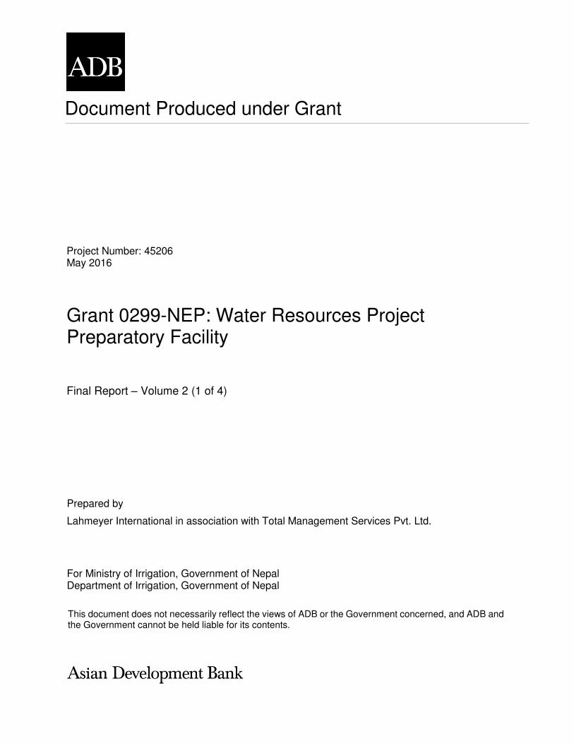
GOVERNMENT OF NEPAL Ministry of Irrigation
Department of Water Induced Disaster Prevention
Technical Assistance Consultant’s Report
Grant No. 0299-NEP: Water Resources Project Preparatory Facility May 2016
Package 3: Flood Hazard Mapping and Preliminary Preparation of Flood Risk Management Projects
Prepared by Lahmeyer International
in association with Total Management Services
Final Report – VOLUME 2
GOVERNMENT OF NEPAL
Ministry of Irrigation
Department of Water Induced Disaster Prevention
FINAL REPORT
VOLUME 2
APPENDIX A – RAINFALL ANALYSIS AND CLIMATE CHANGE TRENDS
APPENDIX B – HYDROLOGICAL ANALYSIS AND MODELLING
Water Resources Project Preparatory Facility
Package 3: Flood Hazard Mapping and Preliminary Preparation of Flood Risk Management Projects
Grant No. 0299-NEP
MAY 2016

This consultant’s report does not necessarily reflect the views of the ADB or the Government concerned, and ADB and the Government cannot be held liable for its contents. All the views
expressed herein may not be incorporated into the proposed project’s design.
WRPPF-Package 3: Flood Hazard Mapping & Preliminary Preparation of Risk Management Projects i Final Report May 2016
Volume 2: Appendix A Lahmeyer International in association with Total Management Services
CONTENTS
VOLUME 1
MAIN REPORT
VOLUME 2
APPENDIX A – RAINFALL ANALYSIS AND CLIMATE CHANGE TRENDS
APPENDIX B – HYDROLOGICAL ANALYSIS AND MODELLING
VOLUME 3
APPENDIX C – HYDRAULIC MODELLING, HAZARD AND RISK MAPPING
VOLUME 4
APPENDIX D – BASIN SCREENING AND RANKING
APPENDIX E – CONCEPT NOTES FOR BIRING BASIN APPENDIX F – CONCEPT NOTES FOR MAWA RATUWA BASIN
VOLUME 5
APPENDIX G – CONCEPT NOTES FOR LAKHANDEHI BASIN APPENDIX H – CONCEPT NOTES FOR EAST RAPTI BASIN APPENDIX I – CONCEPT NOTES FOR WEST RAPTI BASIN APPENDIX J – CONCEPT NOTES FOR MOHANA BASIN

WRPPF-Package 3: Flood Hazard Mapping & Preliminary Preparation of Risk Management Projects ii Final Report May 2016
Volume 2: Appendix A Lahmeyer International in association with Total Management Services
APPENDIX A
RAINFALL ANALYSIS AND CLIMATE CHANGE TRENDS
CONTENTS
I. RAINFALL EVALUATION ..................................................................................................... 1
Physiographic controls upon the rainfall distribution .................................................... 1 Raingauge Network Density ......................................................................................... 4 Sample interstation correlations (24 hours) for the Terai ............................................. 4
II. CLIMATE CHANGE EFFECTS UPON THE RAINFALL ...................................................... 7
GCM Projections .......................................................................................................... 7 AR4 Output from DHM Climate Portal ................................................................ 7 AR5 GCMs from World Bank Climate Change Knowledge Portal ..................... 9 CMIP5 (AR5) ....................................................................................................... 9
The Validity of GCM Results with respect to Flood Calculations ............................... 16 Evidence Based Instrumental Trend Analysis ............................................................ 17
Single Station Rainfall Trends .......................................................................... 17 Inter-Study Comparison .............................................................................................. 26 24-Hour Maximum Rainfall ......................................................................................... 27
III. RAINFALL INPUT FOR BASIN-RUNOFF MODELLING .................................................... 29
IV. CONCLUSIONS ................................................................................................................... 31
V. REFERENCES ..................................................................................................................... 32
ANNEX 1: MONTHLY RAINFALL SUMMARIES ......................................................................... 33
WRPPF-Package 3: Flood Hazard Mapping & Preliminary Preparation of Risk Management Projects iii Final Report May 2016
Volume 2: Appendix A Lahmeyer International in association with Total Management Services
LIST OF FIGURES
Figure 1: Location of rainfall stations for rainfall-altitude analysis ................................................... 1 Figure 2: Face-value mean rainfall-altitude relationship .................................................................. 3 Figure 3: Semi-Variogram of Stations in the Terai and Siwaliks ...................................................... 6 Figure 4: Various climate change scenarios .................................................................................... 8 Figure 5: Stations representing grid in Terai .................................................................................. 11 Figure 6: Historic and projected rainfall (RCP2.6) for July ............................................................. 11 Figure 7: Historic and Projected rainfall (RCP4.5) for July ............................................................ 12 Figure 8: Historic and Projected rainfall (RCP4.5) for July ............................................................ 12 Figure 9: Grids representing Himalayan area ................................................................................ 13 Figure 10: Percentage Increase in Rainfall (RCP4.5) .................................................................... 14 Figure 11: Face-value means of annual and monsoonal variation + second order trend
(station 1216 Siraha) ...................................................................................................... 17 Figure 12: Face-value means of annual and monsoonal variation + second order trend
(station 1408 Damak) ..................................................................................................... 18 Figure 13: Face-value means of annual and monsoonal variation + second order trend
(station 1110 Tulsi) ......................................................................................................... 19 Figure 14: Face-value means of annual and monsoonal variation + second order trend
(station 911 Parwanipur)................................................................................................. 20 Figure 15: Annual 24-hour maxima (station 1408 Damak) ............................................................ 21 Figure 16: Annual 24-hour maxima (station 1216 Siraha) ............................................................. 22 Figure 17: Annual 24-hour maxima (station 1110 Tulsi) ................................................................ 22 Figure 18: Annual 24-hour maxima (station 911 Parwanipur) ....................................................... 23 Figure 19: Location of stations for trend analysis .......................................................................... 23 Figure 20: 24-hour maxima Rainfall Trends: 17 stations in the Terai and Siwaliks ....................... 25 Figure 21: 24-hr Rainfall Frequencies: Station 405, Chisapani Karnali ......................................... 27 Figure 22: 24-hr Rainfall Frequencies: Station 911, Parwanipur ................................................... 28 Figure 23: 24-hr Rainfall Frequencies: Station 1216, Siraha ......................................................... 28
WRPPF-Package 3: Flood Hazard Mapping & Preliminary Preparation of Risk Management Projects iv Final Report May 2016
Volume 2: Appendix A Lahmeyer International in association with Total Management Services
LIST OF TABLES
Table 1: List of stations for rainfall-altitude analysis ........................................................................ 2 Table 2: Network density for Nepal .................................................................................................. 4 Table 3: List of stations for interstation correlation analysis ............................................................ 5 Table 4: Interstation correlations ...................................................................................................... 5 Table 5: Interstation distances (km) ................................................................................................. 5 Table 6: Annual Rainfall averaged over Nepal region from observations and models .................... 8 Table 7: List of stations for comparison ......................................................................................... 10 Table 8: CMIP5: Sixteen GCM comparisons for east to west stations along the Terai
(numbered on map) ........................................................................................................ 10 Table 9: Increases in Rainfall based upon CMIP5 – 16 model ensemble medians,
RCP4.5 for July ............................................................................................................... 13 Table 10: 16-Model-based Rainfall increases (%) from Climate Change, RCP4.5 ....................... 15 Table 11: Ranges of extreme modelled rainfall ............................................................................. 16 Table 12: Summary of monsoon rainfall trends from long-period, low-fragmented
station records ................................................................................................................ 20 Table 13: Summary of monsoon rainfall trends from 24-hour maxima, low-fragmented
station records ................................................................................................................ 21 Table 14: List of stations for trend analysis .................................................................................... 24 Table 15: Result of trend analysis .................................................................................................. 24 Table 16: Terai Rainfall Projections (monsoon season) based upon instrumental
trends .............................................................................................................................. 25 Table 17: Comparison of data in two studies ................................................................................. 26 Table 18: Adopted mean rainfall-altitude relationships, normalised with respect to the
rainfall at 1000 metres. ................................................................................................... 29 Table 19: Monthly rainfall summary for Damak, Station Nr. 1408 ................................................. 34 Table 20: Monthly rainfall summary for Parwanipur, Station Nr. 911 ............................................ 35 Table 21: Monthly rainfall summary for Tulsi, Station Nr. 1110 ..................................................... 36 Table 22: Monthly rainfall summary for Siraha, Station Nr. 1216 .................................................. 37
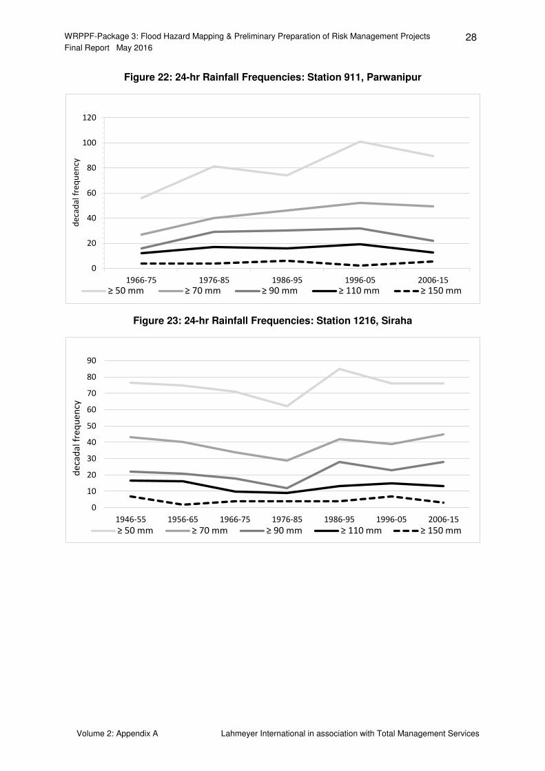
WRPPF-Package 3: Flood Hazard Mapping & Preliminary Preparation of Risk Management Projects 1 Final Report May 2016
Volume 2: Appendix A Lahmeyer International in association with Total Management Services
I. RAINFALL EVALUATION
1. In this section the problems and issues of defining rainfall input are addressed, both
on the assumption of stationarity of the dataset, and incorporating climate change trends.
Physiographic controls upon the rainfall distribution
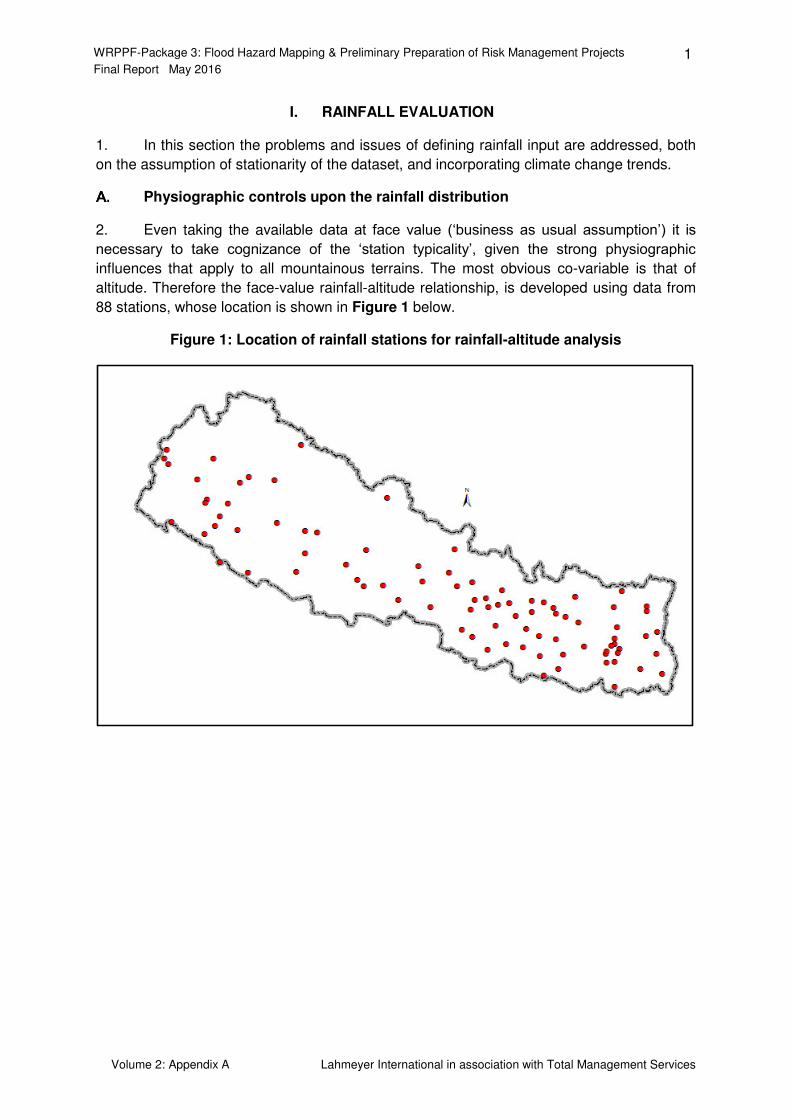
2. Even taking the available data at face value (‘business as usual assumption’) it is necessary to take cognizance of the ‘station typicality’, given the strong physiographic influences that apply to all mountainous terrains. The most obvious co-variable is that of
altitude. Therefore the face-value rainfall-altitude relationship, is developed using data from
88 stations, whose location is shown in Figure 1 below.
Figure 1: Location of rainfall stations for rainfall-altitude analysis
WRPPF-Package 3: Flood Hazard Mapping & Preliminary Preparation of Risk Management Projects 2 Final Report May 2016
Volume 2: Appendix A Lahmeyer International in association with Total Management Services
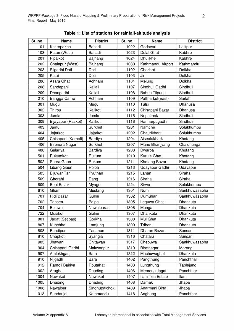
Table 1: List of stations for rainfall-altitude analysis
St. no. Name District St. no. Name District
101 Kakerpakha Baitadi 1022 Godavari Lalitpur
103 Patan (West) Baitadi 1023 Dolal Ghat Kabhre
201 Pipalkot Bajhang 1024 Dhulikhel Kabhre
202 Chainpur (West) Bajhang 1030 Kathmandu Airport Kathmandu
203 Silgadhi Doti Doti 1102 Charikot Dolkha
205 Katai Doti 1103 Jiri Dolkha
206 Asara Ghat Achham 1104 Melung Dolkha
208 Sandepani Kailali 1107 Sindhuli Gadhi Sindhuli
209 Dhangadhi Kaliali 1108 Bahun Tilpung Sindhuli
210 Bangga Camp Achham 1109 Pattharkot(East) Sarlahi
301 Mugu Mugu 1110 Tulsi Dhanusa
302 Thirpu Kalikot 1112 Chisapani Bazar Dhanusa
303 Jumla Jumla 1115 Nepalthok Sindhuli
309 Bijayapur (Raskot) Kalikot 1116 Hariharpugadhi Sindhuli
403 Jamu Surkhet 1201 Namche Solukhumbu
404 Jajarkot Jajarkot 1202 Chaurikhark Solukhumbu
405 Chisapani (Karnali) Bardiya 1204 Aisealukhark Khotang
406 Birendra Nagar Surkhet 1207 Mane Bhanjyang Okaldhunga
408 Gulariya Bardiya 1208 Dwarpa Khotang
501 Rukumkot Rukum 1210 Kurule Ghat Khotang
502 Shera Gaun Rukum 1211 Khotang Bazar Khotang
504 Libang Gaun Rolpa 1213 Udayapur Gadhi Udayapur
505 Bijuwar Tar Pyuthan 1215 Lahan Siraha
509 Ghorahi Dang 1216 Siraha Siraha
609 Beni Bazar Myagdi 1224 Sirwa Solukhumbu
610 Ghami Mustang 1301 Num Sankhuwasabha
701 Ridi Bazar Gulmi 1302 Dumuhan Sankhuwasabha
702 Tansen Palpa 1305 Leguwa Ghat Dhankuta
704 Beluwa Nawalparasi 1306 Munga Dhankuta
722 Musikot Gulmi 1307 Dhankuta Dhankuta
801 Jagat (Setibas) Gorkha 1308 Mul Ghat Dhankuta
807 Kunchha Lamjung 1309 Tribeni Dhankuta
808 Bandipur Tanahun 1311 Dharan Bazar Sunsari
810 Chapkot Syangja 1316 Chatara Sunsari
903 Jhawani Chitawan 1317 Chepuwa Sankhuwasabha
904 Chisapani Gadhi Makwanpur 1319 Biratnagar Morang
907 Amlekhganj Bara 1322 Machuwaghat Dhankuta
910 Nijgadh Bara 1402 Pangthung Panchthar
912 Ramoli Bairiya Routahat 1403 Lungthung Taplejung
1002 Arughat Dhading 1406 Memeng Jagat Panchthar
1004 Nuwakot Nuwakot 1407 Ilam Tea Estate Ilam
1005 Dhading Dhading 1408 Damak Jhapa
1008 Nawalpur Sindhupalchok 1409 Anarmani Birta Jhapa
1013 Sundarijal Kathmandu 1418 Angbung Panchthar
WRPPF-Package 3: Flood Hazard Mapping & Preliminary Preparation of Risk Management Projects 3 Final Report May 2016
Volume 2: Appendix A Lahmeyer International in association with Total Management Services
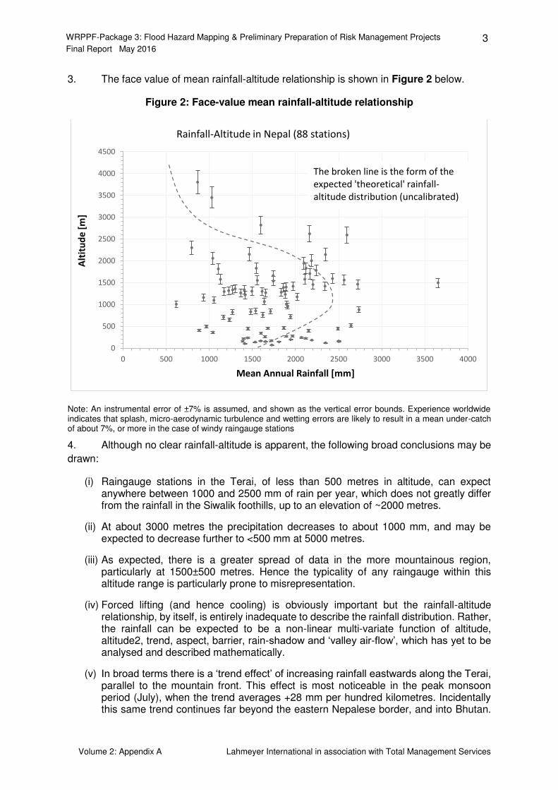
3. The face value of mean rainfall-altitude relationship is shown in Figure 2 below.
Figure 2: Face-value mean rainfall-altitude relationship
Note: An instrumental error of ±7% is assumed, and shown as the vertical error bounds. Experience worldwide indicates that splash, micro-aerodynamic turbulence and wetting errors are likely to result in a mean under-catch of about 7%, or more in the case of windy raingauge stations
4. Although no clear rainfall-altitude is apparent, the following broad conclusions may be
drawn:
(i) Raingauge stations in the Terai, of less than 500 metres in altitude, can expect anywhere between 1000 and 2500 mm of rain per year, which does not greatly differ from the rainfall in the Siwalik foothills, up to an elevation of ~2000 metres.
(ii) At about 3000 metres the precipitation decreases to about 1000 mm, and may be expected to decrease further to <500 mm at 5000 metres.
(iii) As expected, there is a greater spread of data in the more mountainous region, particularly at 1500±500 metres. Hence the typicality of any raingauge within this altitude range is particularly prone to misrepresentation.
(iv) Forced lifting (and hence cooling) is obviously important but the rainfall-altitude relationship, by itself, is entirely inadequate to describe the rainfall distribution. Rather, the rainfall can be expected to be a non-linear multi-variate function of altitude, altitude2, trend, aspect, barrier, rain-shadow and ‘valley air-flow’, which has yet to be analysed and described mathematically.
(v) In broad terms there is a ‘trend effect’ of increasing rainfall eastwards along the Terai, parallel to the mountain front. This effect is most noticeable in the peak monsoon period (July), when the trend averages +28 mm per hundred kilometres. Incidentally this same trend continues far beyond the eastern Nepalese border, and into Bhutan.
0
500
1000
1500
2000
2500
3000
3500
4000
4500
0 500 1000 1500 2000 2500 3000 3500 4000
Alt
itu
de
[m
]
Mean Annual Rainfall [mm]
Rainfall-Altitude in Nepal (88 stations)
The broken line is the form of the
expected 'theoretical' rainfall-
altitude distribution (uncalibrated)

WRPPF-Package 3: Flood Hazard Mapping & Preliminary Preparation of Risk Management Projects 4 Final Report May 2016
Volume 2: Appendix A Lahmeyer International in association with Total Management Services
This trend effect is at least as strong as, if not much stronger than, the altitude effect, but may be masked on the meso-scale by local physiographic effects. These meso-scale rainfall variations cannot be satisfactorily represented with the existing raingauge network density.
5. Other physiographic effects which are very strong include ‘aspect’, ‘rain-shadow’ and ‘barrier effects’ of successive ranges of hills of similar mean altitude. For example, Singh et al
(2001) emphasised the strong rain-shadow and barrier effects in reporting on the middle
Himalayas, where the rainfall gradient is 106 mm /100m on windward slopes, as opposed to
13 mm / 100m on leeward slopes. This severely impacts upon the choice of design rainfall
amounts, as discussed below under ‘rainfall input for basin-runoff modelling’.
Raingauge Network Density
6. As in almost all countries, the logistics, and in particular the cost of maintaining a
network, results in the national network being very much sub-optimal for water resources and
flood estimation work. The network density for Nepal is given in Table 2 below:
Table 2: Network density for Nepal
Terrain Total area, km2 Network total, Φ Network density, §
All Nepal 147,000 264 550
Terai 25,000 67 370
Siwaliks and low Himalayas 40,000 92 430
Optimum raingauge density ʯ - About 20 to 45
Φ Long period raingauges in the National Hydrometric Network.
§ Average area, Km2 represented by each gauge.
ʯ The optimum raingauge density in mountainous environments is not amenable to precise characterisation.
This estimate is based upon several research reports, such as that of Lopez et al., (2015), Volkman et al.
(2010).
7. The ability to infer spatially distributed data from point measurements is strongly
dependent on the number, location and reliability of measurement stations. In general the
WMO recommendations for the ideal minimum raingauge density in tropical mountain areas
is one station per 100 to 250 km2, and the acceptable density of one station per 250 to 1000
km2. We regard these as too generous for the complex physiographic controls which prevail
in the project area. In particular, we note that a reduced rain gauge network density in the
higher parts of the catchment results in a noticeable decline in performance indices.
8. The Bureau of Indian Standards recommends a minimum raingauge density, in hilly
areas with heavy rain, of 130 km2 per gauge.
Sample interstation correlations (24 hours) for the Terai
9. For accurate rainfall estimation, the clearest indication of required network density is
inferred from the interstation correlations. Hence, the Pearson moment correlations for non-
zero rain-days is given for 9 raingauge stations with long periods of record, mainly in the Terai.
WRPPF-Package 3: Flood Hazard Mapping & Preliminary Preparation of Risk Management Projects 5 Final Report May 2016
Volume 2: Appendix A Lahmeyer International in association with Total Management Services
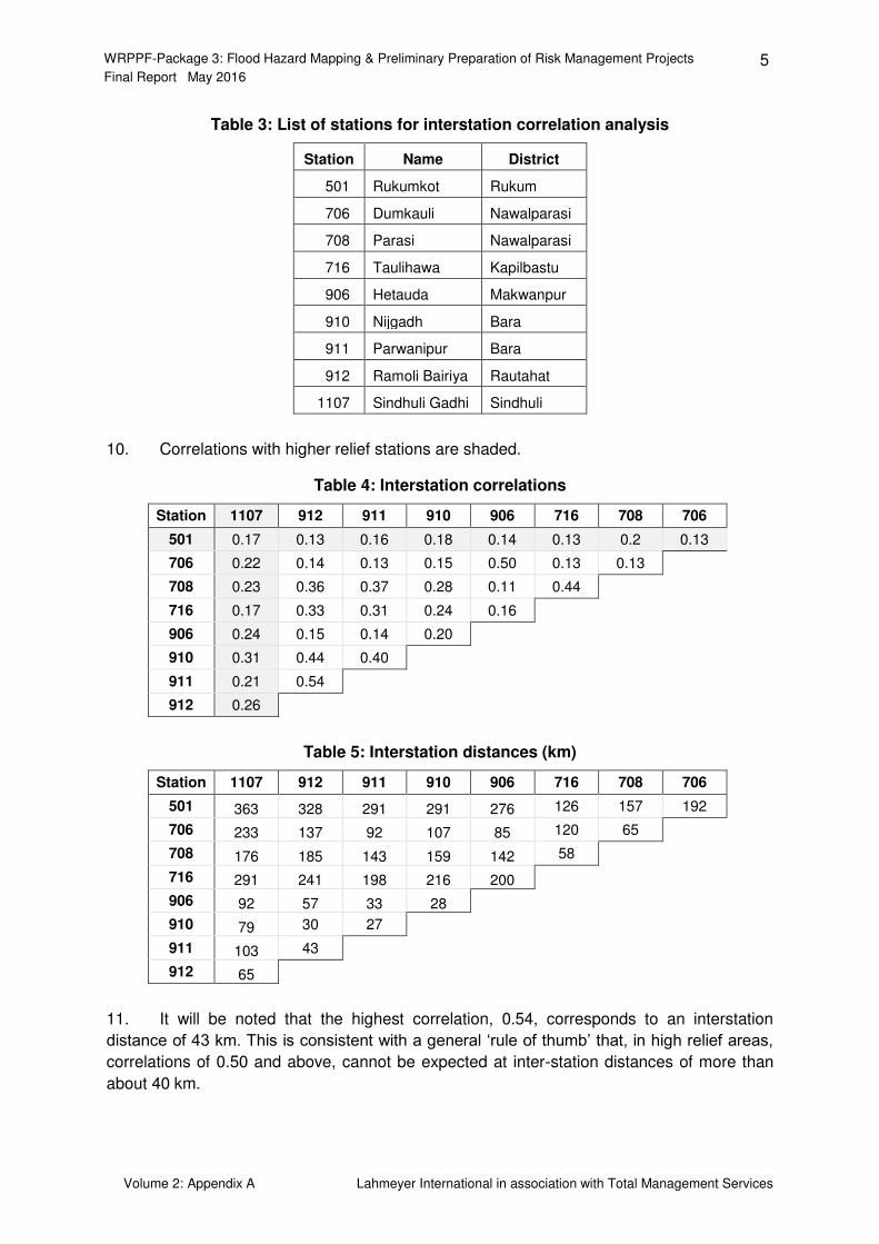
Table 3: List of stations for interstation correlation analysis
Station Name District
501 Rukumkot Rukum
706 Dumkauli Nawalparasi
708 Parasi Nawalparasi
716 Taulihawa Kapilbastu
906 Hetauda Makwanpur
910 Nijgadh Bara
911 Parwanipur Bara
912 Ramoli Bairiya Rautahat
1107 Sindhuli Gadhi Sindhuli
10. Correlations with higher relief stations are shaded.
Table 4: Interstation correlations
Station 1107 912 911 910 906 716 708 706
501 0.17 0.13 0.16 0.18 0.14 0.13 0.2 0.13
706 0.22 0.14 0.13 0.15 0.50 0.13 0.13
708 0.23 0.36 0.37 0.28 0.11 0.44
716 0.17 0.33 0.31 0.24 0.16
906 0.24 0.15 0.14 0.20
910 0.31 0.44 0.40
911 0.21 0.54
912 0.26
Table 5: Interstation distances (km)
Station 1107 912 911 910 906 716 708 706
501 363 328 291 291 276 126 157 192
706 233 137 92 107 85 120 65
708 176 185 143 159 142 58
716 291 241 198 216 200
906 92 57 33 28
910 79 30 27
911 103 43
912 65
11. It will be noted that the highest correlation, 0.54, corresponds to an interstation
distance of 43 km. This is consistent with a general ‘rule of thumb’ that, in high relief areas, correlations of 0.50 and above, cannot be expected at inter-station distances of more than
about 40 km.
WRPPF-Package 3: Flood Hazard Mapping & Preliminary Preparation of Risk Management Projects 6 Final Report May 2016
Volume 2: Appendix A Lahmeyer International in association with Total Management Services
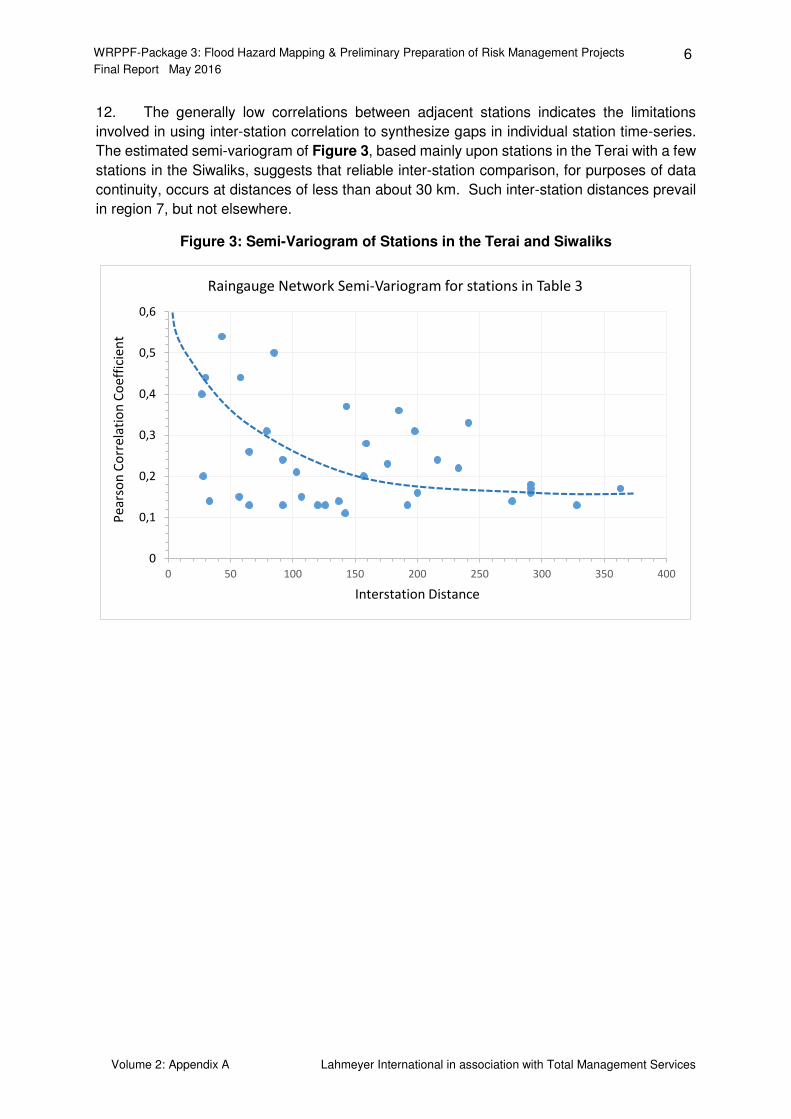
12. The generally low correlations between adjacent stations indicates the limitations
involved in using inter-station correlation to synthesize gaps in individual station time-series.
The estimated semi-variogram of Figure 3, based mainly upon stations in the Terai with a few
stations in the Siwaliks, suggests that reliable inter-station comparison, for purposes of data
continuity, occurs at distances of less than about 30 km. Such inter-station distances prevail
in region 7, but not elsewhere.
Figure 3: Semi-Variogram of Stations in the Terai and Siwaliks
0
0,1
0,2
0,3
0,4
0,5
0,6
0 50 100 150 200 250 300 350 400
Pe
ars
on
Co
rre
lati
on
Co
eff
icie
nt
Interstation Distance
Raingauge Network Semi-Variogram for stations in Table 3

WRPPF-Package 3: Flood Hazard Mapping & Preliminary Preparation of Risk Management Projects 7 Final Report May 2016
Volume 2: Appendix A Lahmeyer International in association with Total Management Services
II. CLIMATE CHANGE EFFECTS UPON THE RAINFALL
13. In principle, the indisputable overall global warming will have the effect of increasing
the precipitable moisture, and hence the rain over the lower Himalayas of Nepal. On the other
hand the redistribution of South Asian circulation could have a reverse effect by either
weakening or redistribution the monsoonal airflow. Despite decades of gradually improving
AOGCMs, the relative dominance of these conflicting processes is still unresolved. Forward
projections of rainfall variation due to climate change are always difficult to assess, and doubly
so in the case of the Indian Monsoonal region. Currently the quantitative impact of global
warming upon the Himalayan monsoonal rainfall is one of the great unanswered questions of
climate change science, in which no definitive quantitative assessments are yet possible.
Therefore, there is a range of semi-quantitative indications in which a provisional consensus
is the best that can be accessed for technical planning purposes.
14. It is most unfortunate that global climatic models (GCMs), or their downscaled
derivatives have come to be relied upon as the sole predictor of climate-change induced
rainfall trends. This is like ‘putting all one’s eggs in a basket –with holes’. Since all the methodologies have their limitations with respect to the requisite reliability it is prudent to
assess the rainfall trends from as many perspectives as possible.
15. There are at least four possible approaches:
(i) GCM projections
(ii) Evidence based instrumental trend analysis
(iii) Precipitable moisture profiling, and
(iv) Depth-duration envelope drift.
16. Unfortunately the relevant data were not available to undertake methods 3 and 4, and
consequently this study is limited to only two approaches, with all the implicit uncertainties that
these entail.
GCM Projections
17. In order to assess the internal consistency of the modelling approach, two sets of
GCMs were analysed separately, effectively as two independent studies. The first of these
was the climate portal posted by the Nepal Department of Hydrology and Meteorology (DHM),
and the second was another climate change portal for southern Asia, hosted by the World
Bank.
AR4 Output from DHM Climate Portal
18. The DHM climate portal uses the following regional climatic models (RCMs): PRECIS,
based upon the atmospheric component of HadCM3; RegCM4, and WRF4. These model
simulations are based upon the IPCC 4th assessment (AR4), and are now superseded by the
5th assessment (AR5). They are here regarded as less reliable than the AR5 experimental
data. Nevertheless, the data of Table 6 yields a ‘first pass’ in which the mean ratio of forward
projected rainfall to historic rainfall was 1.034. The baseline data employed was 1971 to 2000,
and the simulation period was 2030 to 2060.
WRPPF-Package 3: Flood Hazard Mapping & Preliminary Preparation of Risk Management Projects 8 Final Report May 2016
Volume 2: Appendix A Lahmeyer International in association with Total Management Services
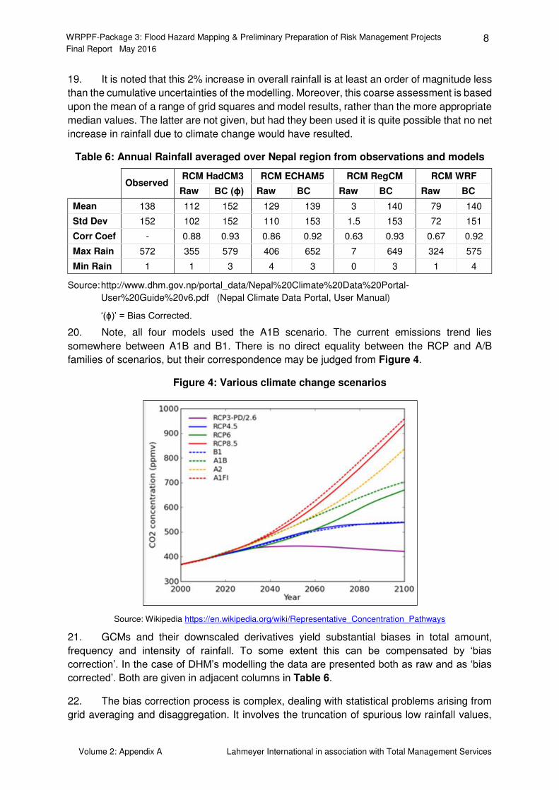
19. It is noted that this 2% increase in overall rainfall is at least an order of magnitude less
than the cumulative uncertainties of the modelling. Moreover, this coarse assessment is based
upon the mean of a range of grid squares and model results, rather than the more appropriate
median values. The latter are not given, but had they been used it is quite possible that no net
increase in rainfall due to climate change would have resulted.
Table 6: Annual Rainfall averaged over Nepal region from observations and models
Observed
RCM HadCM3 RCM ECHAM5 RCM RegCM RCM WRF
Raw BC (ϕ) Raw BC Raw BC Raw BC
Mean 138 112 152 129 139 3 140 79 140
Std Dev 152 102 152 110 153 1.5 153 72 151
Corr Coef - 0.88 0.93 0.86 0.92 0.63 0.93 0.67 0.92
Max Rain 572 355 579 406 652 7 649 324 575
Min Rain 1 1 3 4 3 0 3 1 4
Source: http://www.dhm.gov.np/portal_data/Nepal%20Climate%20Data%20Portal-
User%20Guide%20v6.pdf (Nepal Climate Data Portal, User Manual)
‘(ϕ)’ = Bias Corrected.
20. Note, all four models used the A1B scenario. The current emissions trend lies
somewhere between A1B and B1. There is no direct equality between the RCP and A/B
families of scenarios, but their correspondence may be judged from Figure 4.
Figure 4: Various climate change scenarios
Source: Wikipedia https://en.wikipedia.org/wiki/Representative_Concentration_Pathways
21. GCMs and their downscaled derivatives yield substantial biases in total amount,
frequency and intensity of rainfall. To some extent this can be compensated by ‘bias correction’. In the case of DHM’s modelling the data are presented both as raw and as ‘bias corrected’. Both are given in adjacent columns in Table 6.
22. The bias correction process is complex, dealing with statistical problems arising from
grid averaging and disaggregation. It involves the truncation of spurious low rainfall values,
WRPPF-Package 3: Flood Hazard Mapping & Preliminary Preparation of Risk Management Projects 9 Final Report May 2016
Volume 2: Appendix A Lahmeyer International in association with Total Management Services
and applies an empirical distribution of historic rainfall to the modelled rainfall intensities.
Although the bias corrected data are more consistent with the historic data, the correction
process has the effect of introducing a new level of uncertainty, comparable in magnitude to
the RCM spread of the climate projections, and hence must be treated with caution.
23. Analysis of the HADGEM2 (Hadley Centre Model of UK Met office) climate model, and
their application in terms of estimated 24-hour maximum rainfall, for the RCP4.5 scenario,
yields the following mean rates of increasing rainfall (assuming linear growth):
West Rapti +2.0 mm per decade Mawa Ratuwa +2.3 mm per decade Jhim +6.8 mm per decade
24. These are very modest rainfall growth rates compared to basins with a significant
fraction in the ‘Himalayan’ zone, discussed below.
AR5 GCMs from World Bank Climate Change Knowledge Portal
25. The usual GCM approach is to assume a climatic evolutionary scenario, and to
undertake modelling using a wide range of models and implicit assumptions.
26. Three scenarios were used in this study, RCPs 2.6, 4.5 and 8.5, in which the numbers
refer to the radiative forcing in +W.m-2. Of these the 8.5 is probably unduly pessimistic. The
2.6 is now probably unachievable (due to slow international response on emissions), which
leaves the 4.5 scenario as probably close to the realistic likely emissions trend. The RCP
trends are summarised in Figure 4.
27. There is a disconcerting array of over 20 GCMs which yield widely disparate forward
modelled projections. Realistic error bounds have not been quoted for these models.
CMIP5 (AR5)
28. As a check upon the DHM’s results, the computer modelling over a different set of
models utilized the Coupled Model Inter-comparison Project Phase 5, usually known as
‘CMIP5’, was used to assess the overall most likely rainfall trends over the following averaged time steps: historical data up to 2009, 2020 to 2039, 2040 to 2059 and 2060 to 2079. This was
repeated for scenarios RCP2.6, RCP 4.5 and RCP 8.5.
29. CMIP5 uses up to 20 models, used by dozens of modelling groups worldwide. Of these
models, the 16 used in this analysis were as specified under the World Bank Climate Change
Knowledge Portal, details of which may be accessed at:
http://sdwebx.worldbank.org/climateportal/index.cfm?page=resource#user_guide. Or
http://sdwebx.worldbank.org/climateportal/documents/WB_Climate_Change_Knowledge_Portal
_UsersGuide.pdf
30. All of these models are based upon a grid zone of about 90 x 90 km. In order to assess
the likely geographic variation along the Terai, eight raingauge stations were selected from
WNW to ESE as being representative of the eight grid zones. These nominal stations are
numbered 105, 209, 409, 510, 711, 911, 1216, and 1313. It is important to note that, for the
purposes of modelling they are not point rainfall estimates, but averaged grid square rainfalls.
WRPPF-Package 3: Flood Hazard Mapping & Preliminary Preparation of Risk Management Projects 10 Final Report May 2016
Volume 2: Appendix A Lahmeyer International in association with Total Management Services
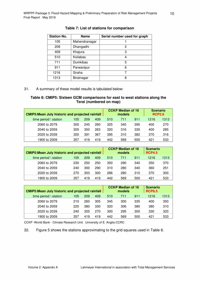
Table 7: List of stations for comparison
Station No. Name Serial number used for graph
105 Mahendranagar 1
209 Dhangadhi 2
409 Khajura 3
510 Koilabas 4
711 Dumkibas 5
911 Parwanipur 6
1216 Siraha 7
1313 Biratnagar 8
31. A summary of these model results is tabulated below:
Table 8: CMIP5: Sixteen GCM comparisons for east to west stations along the Terai (numbered on map)
CMIP5:Mean July historic and projected rainfall CCKP Median of 16
models Scenario RCP2.6
time period \ station 105 209 409 510 711 911 1216 1313
2060 to 2079 300 245 260 325 340 395 400 270
2040 to 2059 305 350 263 320 316 330 400 285
2020 to 2039 320 391 367 395 310 382 370 316
1900 to 2009 357 419 419 442 569 500 421 533
CMIP5:Mean July historic and projected rainfall CCKP Median of 16
models Scenario RCP4.5
time period \ station 105 209 409 510 711 911 1216 1313
2060 to 2079 230 250 250 350 290 340 350 370
2040 to 2059 240 300 290 310 280 340 360 251
2020 to 2039 270 303 300 286 280 310 370 300
1900 to 2009 357 419 419 442 569 500 421 533
CMIP5:Mean July historic and projected rainfall CCKP Median of 16
models Scenario RCP8.5
time period \ station 105 209 409 510 711 911 1216 1313
2060 to 2079 210 260 305 345 300 335 400 350
2040 to 2059 220 380 330 320 306 380 380 310
2020 to 2039 240 355 270 300 295 300 330 320
1900 to 2009 357 419 419 442 569 500 421 533
CCKP -World Bank - Climate Research Unit. University of E. Anglia-CCRC
32. Figure 5 shows the stations approximating to the grid squares used in Table 8.
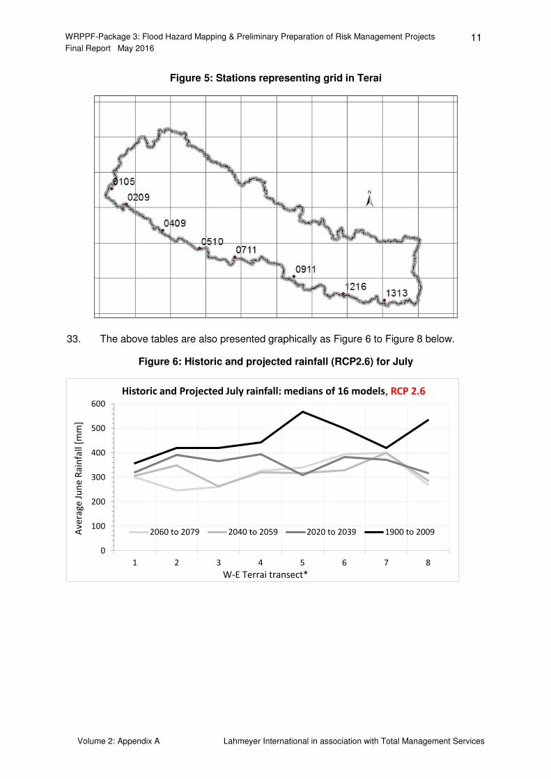
WRPPF-Package 3: Flood Hazard Mapping & Preliminary Preparation of Risk Management Projects 11 Final Report May 2016
Volume 2: Appendix A Lahmeyer International in association with Total Management Services
Figure 5: Stations representing grid in Terai
33. The above tables are also presented graphically as Figure 6 to Figure 8 below.
Figure 6: Historic and projected rainfall (RCP2.6) for July
0
100
200
300
400
500
600
1 2 3 4 5 6 7 8
Ave
rag
e J
un
e R
ain
fall
[mm
]
W-E Terrai transect*
Historic and Projected July rainfall: medians of 16 models, RCP 2.6
2060 to 2079 2040 to 2059 2020 to 2039 1900 to 2009
WRPPF-Package 3: Flood Hazard Mapping & Preliminary Preparation of Risk Management Projects 12 Final Report May 2016
Volume 2: Appendix A Lahmeyer International in association with Total Management Services
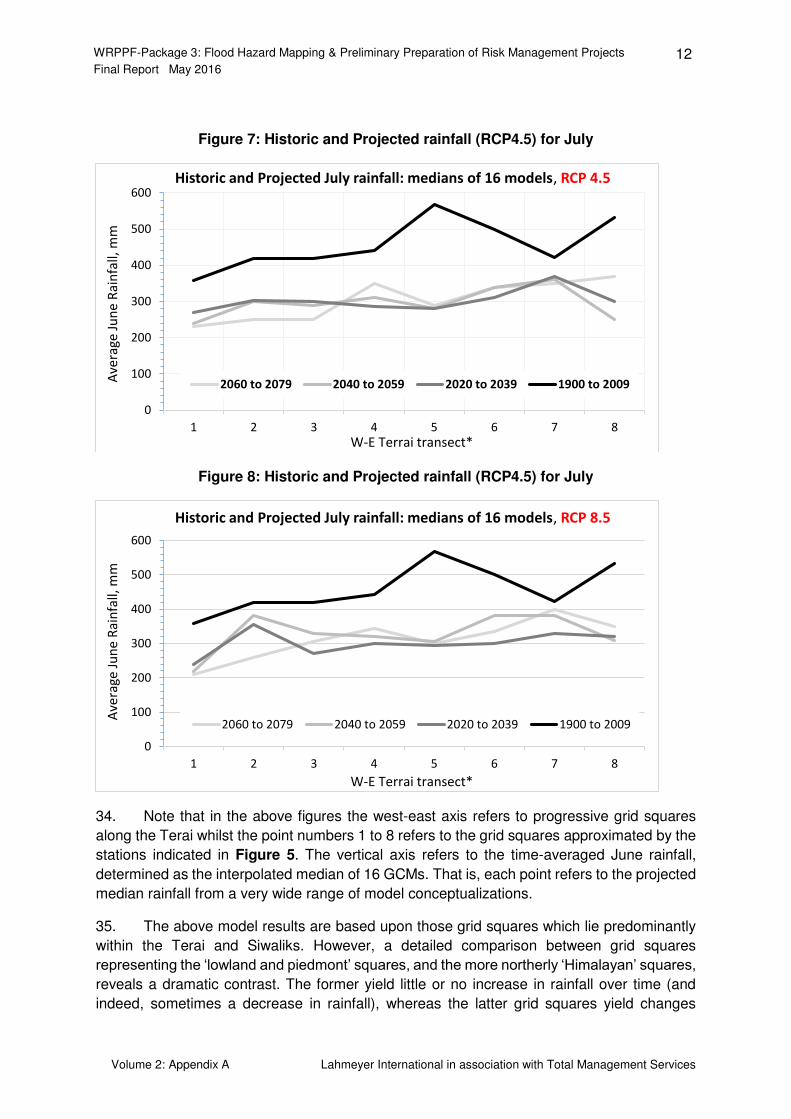
Figure 7: Historic and Projected rainfall (RCP4.5) for July
Figure 8: Historic and Projected rainfall (RCP4.5) for July
34. Note that in the above figures the west-east axis refers to progressive grid squares
along the Terai whilst the point numbers 1 to 8 refers to the grid squares approximated by the
stations indicated in Figure 5. The vertical axis refers to the time-averaged June rainfall,
determined as the interpolated median of 16 GCMs. That is, each point refers to the projected
median rainfall from a very wide range of model conceptualizations.
35. The above model results are based upon those grid squares which lie predominantly
within the Terai and Siwaliks. However, a detailed comparison between grid squares
representing the ‘lowland and piedmont’ squares, and the more northerly ‘Himalayan’ squares, reveals a dramatic contrast. The former yield little or no increase in rainfall over time (and
indeed, sometimes a decrease in rainfall), whereas the latter grid squares yield changes
0
100
200
300
400
500
600
1 2 3 4 5 6 7 8
Ave
rag
e J
un
e R
ain
fall,
mm
W-E Terrai transect*
Historic and Projected July rainfall: medians of 16 models, RCP 4.5
2060 to 2079 2040 to 2059 2020 to 2039 1900 to 2009
0
100
200
300
400
500
600
1 2 3 4 5 6 7 8
Ave
rag
e J
un
e R
ain
fall,
mm
W-E Terrai transect*
Historic and Projected July rainfall: medians of 16 models, RCP 8.5
2060 to 2079 2040 to 2059 2020 to 2039 1900 to 2009
WRPPF-Package 3: Flood Hazard Mapping & Preliminary Preparation of Risk Management Projects 13 Final Report May 2016
Volume 2: Appendix A Lahmeyer International in association with Total Management Services
varying between -23% and +128%. The average 39% increase (2020 to 2080, RCP4.5) is
roughly consistent with previous modelling, anecdotal observations and popular perceptions.
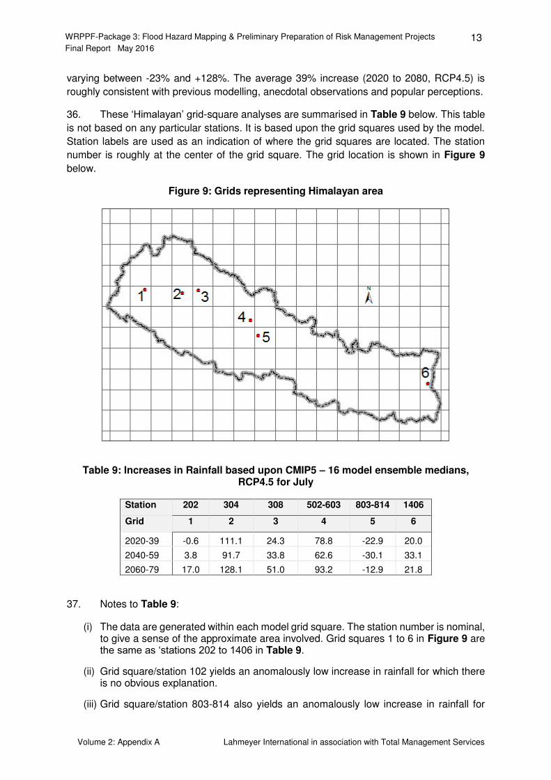
36. These ‘Himalayan’ grid-square analyses are summarised in Table 9 below. This table
is not based on any particular stations. It is based upon the grid squares used by the model.
Station labels are used as an indication of where the grid squares are located. The station
number is roughly at the center of the grid square. The grid location is shown in Figure 9
below.
Figure 9: Grids representing Himalayan area
Table 9: Increases in Rainfall based upon CMIP5 – 16 model ensemble medians, RCP4.5 for July
Station 202 304 308 502-603 803-814 1406
Grid 1 2 3 4 5 6
2020-39 -0.6 111.1 24.3 78.8 -22.9 20.0
2040-59 3.8 91.7 33.8 62.6 -30.1 33.1
2060-79 17.0 128.1 51.0 93.2 -12.9 21.8
37. Notes to Table 9:
(i) The data are generated within each model grid square. The station number is nominal, to give a sense of the approximate area involved. Grid squares 1 to 6 in Figure 9 are the same as ‘stations 202 to 1406 in Table 9.
(ii) Grid square/station 102 yields an anomalously low increase in rainfall for which there is no obvious explanation.
(iii) Grid square/station 803-814 also yields an anomalously low increase in rainfall for
WRPPF-Package 3: Flood Hazard Mapping & Preliminary Preparation of Risk Management Projects 14 Final Report May 2016
Volume 2: Appendix A Lahmeyer International in association with Total Management Services
which there are three evident reasons. Firstly, this grid square has a much lower mean elevation due to the inclusion of almost the entire Kathmandu Valley. Secondly, the grid square is the most southerly of the various ‘Himalayan’ grid squares, incorporating a significant fraction in the Terai. Thirdly, this grid square has a much higher historic rainfall baseline than the other ‘Himalayan’ grid squares, resulting in a negative bias in the percentage increase.
(iv) Of the 16 model results only the median values were considered. Higher increases in rainfall would be indicated if the means were used. Nevertheless, the median values are considered in order to minimize the spurious effects of extreme outlier estimates.
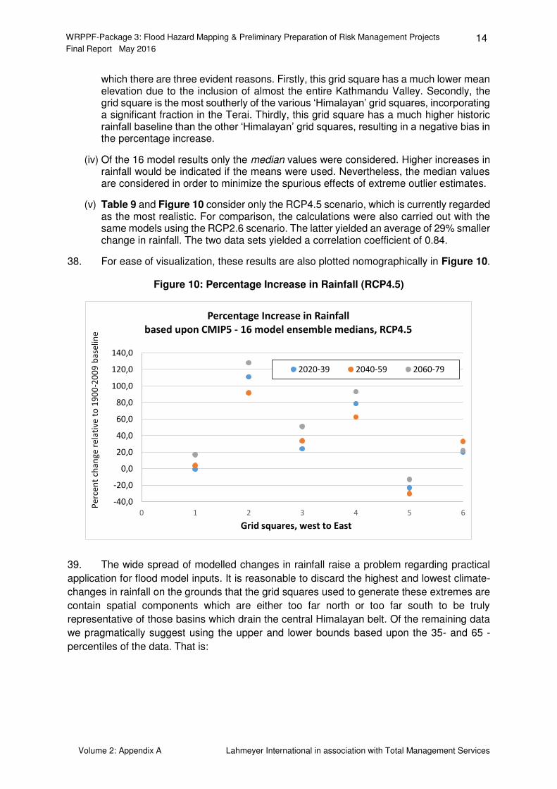
(v) Table 9 and Figure 10 consider only the RCP4.5 scenario, which is currently regarded as the most realistic. For comparison, the calculations were also carried out with the same models using the RCP2.6 scenario. The latter yielded an average of 29% smaller change in rainfall. The two data sets yielded a correlation coefficient of 0.84.
38. For ease of visualization, these results are also plotted nomographically in Figure 10.
Figure 10: Percentage Increase in Rainfall (RCP4.5)
39. The wide spread of modelled changes in rainfall raise a problem regarding practical
application for flood model inputs. It is reasonable to discard the highest and lowest climate-
changes in rainfall on the grounds that the grid squares used to generate these extremes are
contain spatial components which are either too far north or too far south to be truly
representative of those basins which drain the central Himalayan belt. Of the remaining data
we pragmatically suggest using the upper and lower bounds based upon the 35- and 65 -
percentiles of the data. That is:
-40,0
-20,0
0,0
20,0
40,0
60,0
80,0
100,0
120,0
140,0
0 1 2 3 4 5 6
Pe
rce
nt
cha
ng
e r
ela
tive
to
19
00
-20
09
ba
seli
ne
Grid squares, west to East
Percentage Increase in Rainfall
based upon CMIP5 - 16 model ensemble medians, RCP4.5
2020-39 2040-59 2060-79
WRPPF-Package 3: Flood Hazard Mapping & Preliminary Preparation of Risk Management Projects 15 Final Report May 2016
Volume 2: Appendix A Lahmeyer International in association with Total Management Services
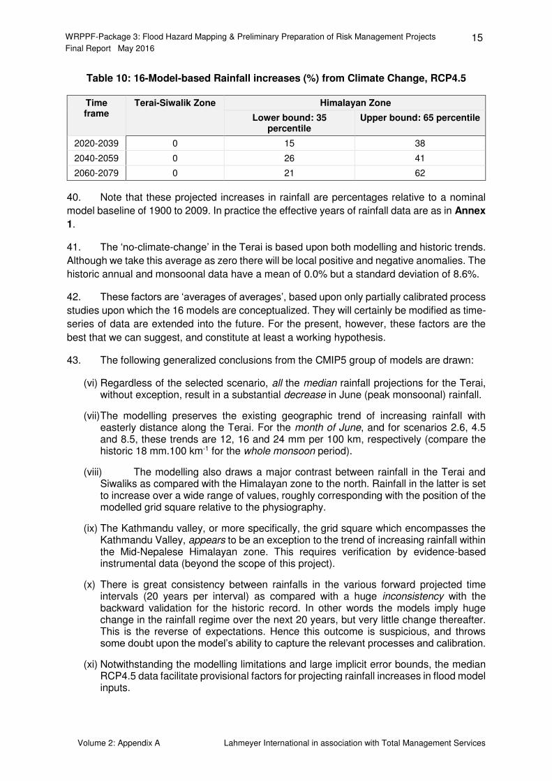
Table 10: 16-Model-based Rainfall increases (%) from Climate Change, RCP4.5
Time frame
Terai-Siwalik Zone Himalayan Zone
Lower bound: 35 percentile
Upper bound: 65 percentile
2020-2039 0 15 38
2040-2059 0 26 41
2060-2079 0 21 62
40. Note that these projected increases in rainfall are percentages relative to a nominal
model baseline of 1900 to 2009. In practice the effective years of rainfall data are as in Annex
1.
41. The ‘no-climate-change’ in the Terai is based upon both modelling and historic trends.
Although we take this average as zero there will be local positive and negative anomalies. The
historic annual and monsoonal data have a mean of 0.0% but a standard deviation of 8.6%.
42. These factors are ‘averages of averages’, based upon only partially calibrated process
studies upon which the 16 models are conceptualized. They will certainly be modified as time-
series of data are extended into the future. For the present, however, these factors are the
best that we can suggest, and constitute at least a working hypothesis.
43. The following generalized conclusions from the CMIP5 group of models are drawn:
(vi) Regardless of the selected scenario, all the median rainfall projections for the Terai, without exception, result in a substantial decrease in June (peak monsoonal) rainfall.
(vii) The modelling preserves the existing geographic trend of increasing rainfall with easterly distance along the Terai. For the month of June, and for scenarios 2.6, 4.5 and 8.5, these trends are 12, 16 and 24 mm per 100 km, respectively (compare the historic 18 mm.100 km-1 for the whole monsoon period).
(viii) The modelling also draws a major contrast between rainfall in the Terai and Siwaliks as compared with the Himalayan zone to the north. Rainfall in the latter is set to increase over a wide range of values, roughly corresponding with the position of the modelled grid square relative to the physiography.
(ix) The Kathmandu valley, or more specifically, the grid square which encompasses the Kathmandu Valley, appears to be an exception to the trend of increasing rainfall within the Mid-Nepalese Himalayan zone. This requires verification by evidence-based instrumental data (beyond the scope of this project).
(x) There is great consistency between rainfalls in the various forward projected time intervals (20 years per interval) as compared with a huge inconsistency with the backward validation for the historic record. In other words the models imply huge change in the rainfall regime over the next 20 years, but very little change thereafter. This is the reverse of expectations. Hence this outcome is suspicious, and throws some doubt upon the model’s ability to capture the relevant processes and calibration.
(xi) Notwithstanding the modelling limitations and large implicit error bounds, the median RCP4.5 data facilitate provisional factors for projecting rainfall increases in flood model inputs.
WRPPF-Package 3: Flood Hazard Mapping & Preliminary Preparation of Risk Management Projects 16 Final Report May 2016
Volume 2: Appendix A Lahmeyer International in association with Total Management Services
The Validity of GCM Results with respect to Flood Calculations
44. These results underscore the basic difficulties of applying GCMs to rainfall trend
prediction. We note the following very important caveats to the modelling results:
45. Caveat 1: None of the AOGCMs or their derivatives are designed for hydrologic
applications, even though that is how they are now often used (misused?). It is therefore
essential to note that such models are highly successful in replicating regional changes in
temperature, but have a much less successful track-record in rainfall. That is, the model
accuracy may be, for example, better than ±0.5°C, whilst outputting worse than ±20% in
rainfall estimation, for the same model simulation.
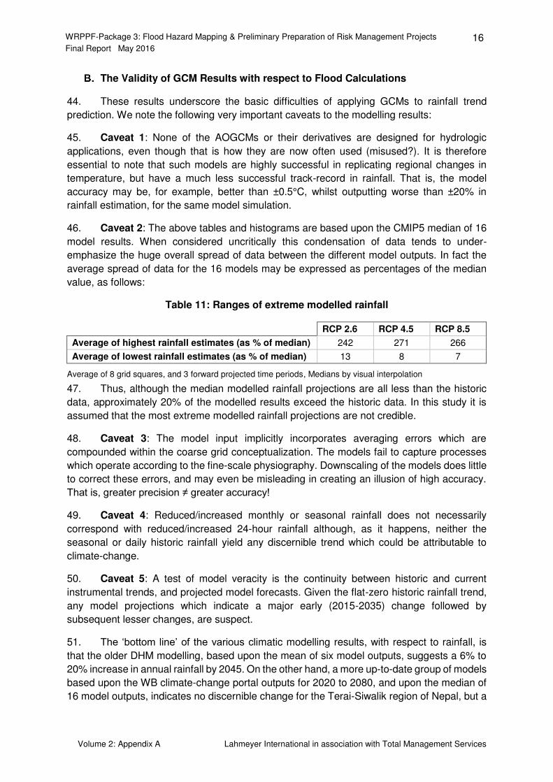
46. Caveat 2: The above tables and histograms are based upon the CMIP5 median of 16
model results. When considered uncritically this condensation of data tends to under-
emphasize the huge overall spread of data between the different model outputs. In fact the
average spread of data for the 16 models may be expressed as percentages of the median
value, as follows:
Table 11: Ranges of extreme modelled rainfall
RCP 2.6 RCP 4.5 RCP 8.5
Average of highest rainfall estimates (as % of median) 242 271 266
Average of lowest rainfall estimates (as % of median) 13 8 7
Average of 8 grid squares, and 3 forward projected time periods, Medians by visual interpolation
47. Thus, although the median modelled rainfall projections are all less than the historic
data, approximately 20% of the modelled results exceed the historic data. In this study it is
assumed that the most extreme modelled rainfall projections are not credible.
48. Caveat 3: The model input implicitly incorporates averaging errors which are
compounded within the coarse grid conceptualization. The models fail to capture processes
which operate according to the fine-scale physiography. Downscaling of the models does little
to correct these errors, and may even be misleading in creating an illusion of high accuracy.
That is, greater precision ≠ greater accuracy!
49. Caveat 4: Reduced/increased monthly or seasonal rainfall does not necessarily
correspond with reduced/increased 24-hour rainfall although, as it happens, neither the
seasonal or daily historic rainfall yield any discernible trend which could be attributable to
climate-change.
50. Caveat 5: A test of model veracity is the continuity between historic and current
instrumental trends, and projected model forecasts. Given the flat-zero historic rainfall trend,
any model projections which indicate a major early (2015-2035) change followed by
subsequent lesser changes, are suspect.
51. The ‘bottom line’ of the various climatic modelling results, with respect to rainfall, is
that the older DHM modelling, based upon the mean of six model outputs, suggests a 6% to
20% increase in annual rainfall by 2045. On the other hand, a more up-to-date group of models
based upon the WB climate-change portal outputs for 2020 to 2080, and upon the median of
16 model outputs, indicates no discernible change for the Terai-Siwalik region of Nepal, but a
WRPPF-Package 3: Flood Hazard Mapping & Preliminary Preparation of Risk Management Projects 17 Final Report May 2016
Volume 2: Appendix A Lahmeyer International in association with Total Management Services
very substantial increase in rainfall for the mid-altitude Himalayan zone immediately
northwards.
Evidence Based Instrumental Trend Analysis
52. Single isolated days of missing data were ‘synthesized’ by comparison or correlation with the two nearest stations wherever the adjacent station-days were <20 mm. Wherever a
missing daily total was bracketed by high rainfall days (>20mm), or occurred during a likely
high rainfall day within the monsoon period, the daily total, and hence monthly total was
regarded as intractable, and hence not included in the time-series analysis. Months with more
than four days of non-zero synthesized data were also considered to be too speculative to be
included in the time-series analysis.
Single Station Rainfall Trends
53. Stations selected for time-trend analysis were severely limited by data availability, data
continuity, durations of data collection, and geographic proximity to basins of interest. In order
of usefulness, the chosen stations were 1216, 1408, 1110 and 911. The monsoon season was
taken as May-September.
a. Station 1216 Siraha
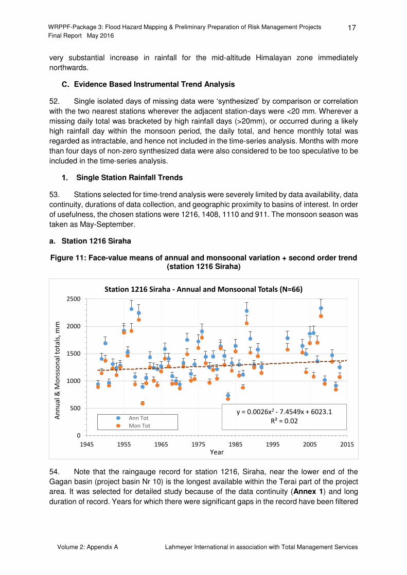
Figure 11: Face-value means of annual and monsoonal variation + second order trend (station 1216 Siraha)
54. Note that the raingauge record for station 1216, Siraha, near the lower end of the
Gagan basin (project basin Nr 10) is the longest available within the Terai part of the project
area. It was selected for detailed study because of the data continuity (Annex 1) and long
duration of record. Years for which there were significant gaps in the record have been filtered
0
500
1000
1500
2000
2500
1945 1955 1965 1975 1985 1995 2005 2015
An
nu
al &
Mo
nss
on
al t
ota
ls, m
m
Year
Station 1216 Siraha - Annual and Monsoonal Totals (N=66)
Ann Tot
Mon Tot
y = 0.0026x2 - 7.4549x + 6023.1
R² = 0.02
WRPPF-Package 3: Flood Hazard Mapping & Preliminary Preparation of Risk Management Projects 18 Final Report May 2016
Volume 2: Appendix A Lahmeyer International in association with Total Management Services
out and were not included in the following calculations. A second order regression of just the
monsoon rainfall indicates: �� = . �2 − . � + .
55. Where RF is the total monsoon rainfall (taken as May to September), and Y is the year.
56. This is an almost linear trend of a slight increase in rainfall over time. However, note
that the ‘R2’ is only 0.02, indicating poor statistical significance, in this case heavily skewed by a quasi-7-year cyclicity of poorly quantified outliers. In the absence of anything better we
have no alternative but to accept this trend as real, but with the caveat that the 95% error
bounds substantially exceed the trend itself, and hance the trend must be regarded as
provisional.
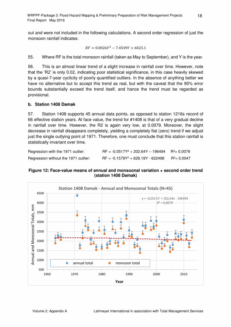
b. Station 1408 Damak
57. Station 1408 supports 45 annual data points, as opposed to station 1216s record of
66 effective station years. At face value, the trend for #1408 is that of a very gradual decline
in rainfall over time. However, the R2 is again very low, at 0.0079. Moreover, the slight
decrease in rainfall disappears completely, yielding a completely flat (zero) trend if we adjust
just the single outlying point of 1971. Therefore, one must conclude that this station rainfall is
statistically invariant over time.
Regression with the 1971 outlier: RF = -0.0517Y2 + 202.64Y – 196494 R2= 0.0079
Regression without the 1971 outlier: RF = -0.1579Y2 + 628.19Y - 622498 R2= 0.0047
Figure 12: Face-value means of annual and monsoonal variation + second order trend (station 1408 Damak)
y = -0,0517x2 + 202,64x - 196494
R² = 0,0079
500
1000
1500
2000
2500
3000
3500
4000
4500
1960 1970 1980 1990 2000 2010
An
nu
al a
nd
Mo
nso
on
al T
ota
ls, m
m
Year
Station 1408 Damak - Annual and Monsoonal Totals (N=45)
annual total monsoon total
WRPPF-Package 3: Flood Hazard Mapping & Preliminary Preparation of Risk Management Projects 19 Final Report May 2016
Volume 2: Appendix A Lahmeyer International in association with Total Management Services
c. Station 1110 Tulsi
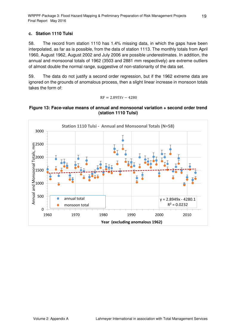
58. The record from station 1110 has 1.4% missing data, in which the gaps have been
interpolated, as far as is possible, from the data of station 1113. The monthly totals from April
1960, August 1962, August 2002 and July 2006 are possible underestimates. In addition, the
annual and monsoonal totals of 1962 (3503 and 2881 mm respectively) are extreme outliers
of almost double the normal range, suggestive of non-stationarity of the data set.
59. The data do not justify a second order regression, but if the 1962 extreme data are
ignored on the grounds of anomalous process, then a slight linear increase in monsoon totals
takes the form of:
RF = . Yr −
Figure 13: Face-value means of annual and monsoonal variation + second order trend (station 1110 Tulsi)
y = 2.8949x - 4280.1
R² = 0.02320
500
1000
1500
2000
2500
3000
1960 1970 1980 1990 2000 2010
An
nu
al a
nd
Mo
nso
on
al T
ota
ls, m
m
Year (excluding anomalous 1962)
Station 1110 Tulsi - Annual and Monsoonal Totals (N=58)
annual total
monsoon total
WRPPF-Package 3: Flood Hazard Mapping & Preliminary Preparation of Risk Management Projects 20 Final Report May 2016
Volume 2: Appendix A Lahmeyer International in association with Total Management Services
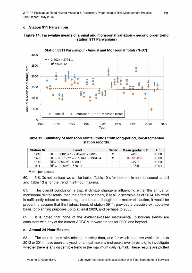
d. Station 911 Parwanipur
Figure 14: Face-value means of annual and monsoonal variation + second order trend (station 911 Parwanipur)
Table 12: Summary of monsoon rainfall trends from long-period, low-fragmented station records
Station Nr Trend Order Mean gradient � R2
1216 RF = 0.0026Y2 - 7.4549Y + 6023 2 +26.5 0.020 1408 RF =-0.0517Y2 + 202.64Y – 196494 2 0.0 to -28.0 0.008
1110 RF= 2.8949Y - 4280.1 1 +27.8 0.023
911 RF = -2.202Y + 5791.1 1 -27.8 0.004 ∇ mm per decade
60. NB: Do not confuse two similar tables: Table 10 is for the trend in net monsoonal rainfall
and Table 13 is for the trend in 24-hour maxima.
61. The overall conclusion is that, if climate change is influencing either the annual or
monsoonal rainfall totals, then the effect is scarcely, if at all, discernible as of 2014. No trend
is sufficiently robust to warrant high credence, although as a matter of caution, it would be
prudent to assume that the highest trend, of station 0911, provides a plausible extrapolative
basis for planning purposes up to at least 2020, and perhaps to 2030.
62. It is noted that none of the evidence–based instrumental (historical) trends are
consistent with any of the current AOGCM forward trends for 2020 and beyond.
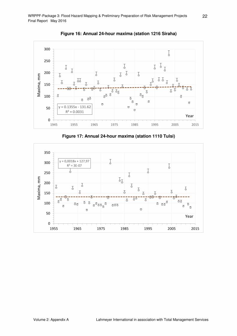
e. Annual 24-Hour Maxima
63. The four stations with minimal missing data, and for which data are available up to
2013 or 2014, have been analysed for annual maxima (not peaks over threshold) to investigate
whether there is any discernible trend in the maximum daily rainfall. These results are plotted
y = -2.202x + 5791.1
R² = 0.0042
0
500
1000
1500
2000
2500
3000
1965 1970 1975 1980 1985 1990 1995 2000 2005
An
nu
al &
Mo
nss
on
al t
ota
ls, m
m
Year
Station 0911 Parwanipur - Annual and Monsoonal Totals (N=37)
annual monsoon monsson trend

WRPPF-Package 3: Flood Hazard Mapping & Preliminary Preparation of Risk Management Projects 21 Final Report May 2016
Volume 2: Appendix A Lahmeyer International in association with Total Management Services
below in Figure 15 to Figure 18. All these time-series are skewed by occasional outliers,
resulting in very low R2 values.
64. It is also noted that identical and consecutive annual 24-hour maxima occur more
frequently that would be expected by chance alone.
Table 13: Summary of monsoon rainfall trends from 24-hour maxima, low-fragmented station records
Station Years Trend Order Mean gradient � R2
1408 50 RF = -0.457Y + 1084.5 1 -4.4 0.014
1216 68 RF = 0.1355Y - 131.62 1 +8.1 0.003
1110 57 RF = 0.0018Y + 127.97 1 0.0 3E-7
0911 47 RF = 0.569Y - 994.89 1 +6.0 0.018 ∇ : mm per decade
65. Clearly there is no consistency of trend, and with such a small sample of stations (with
good record) it is impossible to draw firm conclusions. Ten other stations, with around 5%
missing data yield an apparent mean gradient of +0.7 mm per decade (standard deviation of
8.6 mm).
Figure 15: Annual 24-hour maxima (station 1408 Damak)
y = -0,457x + 1084,5
R² = 0,0142
0
50
100
150
200
250
300
350
400
1960 1970 1980 1990 2000 2010
Ma
xim
a, m
m
Year
WRPPF-Package 3: Flood Hazard Mapping & Preliminary Preparation of Risk Management Projects 22 Final Report May 2016
Volume 2: Appendix A Lahmeyer International in association with Total Management Services
Figure 16: Annual 24-hour maxima (station 1216 Siraha)
Figure 17: Annual 24-hour maxima (station 1110 Tulsi)
y = 0.1355x - 131.62
R² = 0.0031
0
50
100
150
200
250
300
1945 1955 1965 1975 1985 1995 2005 2015
Ma
xim
a, m
m
Year
y = 0,0018x + 127,97
R² = 3E-07
0
50
100
150
200
250
300
350
1955 1965 1975 1985 1995 2005 2015
Ma
xim
a, m
m
Year
WRPPF-Package 3: Flood Hazard Mapping & Preliminary Preparation of Risk Management Projects 23 Final Report May 2016
Volume 2: Appendix A Lahmeyer International in association with Total Management Services
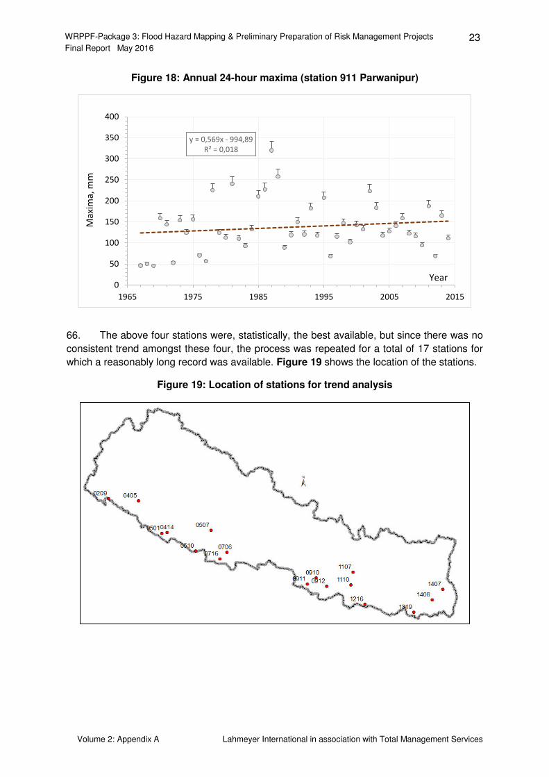
Figure 18: Annual 24-hour maxima (station 911 Parwanipur)
66. The above four stations were, statistically, the best available, but since there was no
consistent trend amongst these four, the process was repeated for a total of 17 stations for
which a reasonably long record was available. Figure 19 shows the location of the stations.
Figure 19: Location of stations for trend analysis
y = 0,569x - 994,89
R² = 0,018
0
50
100
150
200
250
300
350
400
1965 1975 1985 1995 2005 2015
Ma
xim
a, m
m
Year
WRPPF-Package 3: Flood Hazard Mapping & Preliminary Preparation of Risk Management Projects 24 Final Report May 2016
Volume 2: Appendix A Lahmeyer International in association with Total Management Services
Table 14: List of stations for trend analysis
Station Name District
209 Dhangadhi Kaliali
405 Chisapani (Karnali) Bardiya
414 Baijapur Banke
501 Rukumkot Rukum
507 Nayabasti Dang
510 Koilabas Dang
706 Dumkauli Nawalparasi
716 Taulihawa Kapilbastu
910 Nijgadh Bara
911 Parwanipur Bara
912 Ramoli Bairiya Routahat
1107 Sindhuli Gadhi Sindhuli
1110 Tulsi Dhanusa
1216 Siraha Siraha
1319 Biratnagar Morang
1407 Ilam Tea Estate Ilam
1408 Damak Jhapa
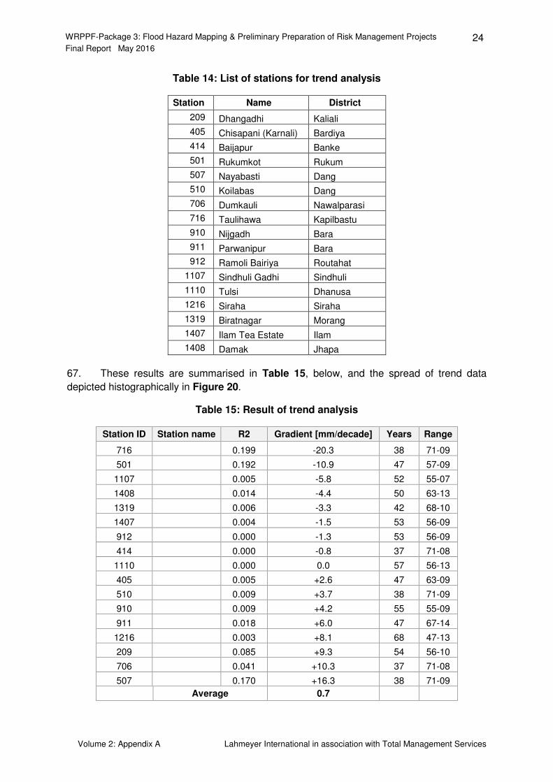
67. These results are summarised in Table 15, below, and the spread of trend data
depicted histographically in Figure 20.
Table 15: Result of trend analysis
Station ID Station name R2 Gradient [mm/decade] Years Range
716 0.199 -20.3 38 71-09
501 0.192 -10.9 47 57-09
1107 0.005 -5.8 52 55-07
1408 0.014 -4.4 50 63-13
1319 0.006 -3.3 42 68-10
1407 0.004 -1.5 53 56-09
912 0.000 -1.3 53 56-09
414 0.000 -0.8 37 71-08
1110 0.000 0.0 57 56-13
405 0.005 +2.6 47 63-09
510 0.009 +3.7 38 71-09
910 0.009 +4.2 55 55-09
911 0.018 +6.0 47 67-14
1216 0.003 +8.1 68 47-13
209 0.085 +9.3 54 56-10
706 0.041 +10.3 37 71-08
507 0.170 +16.3 38 71-09
Average 0.7
WRPPF-Package 3: Flood Hazard Mapping & Preliminary Preparation of Risk Management Projects 25 Final Report May 2016
Volume 2: Appendix A Lahmeyer International in association with Total Management Services
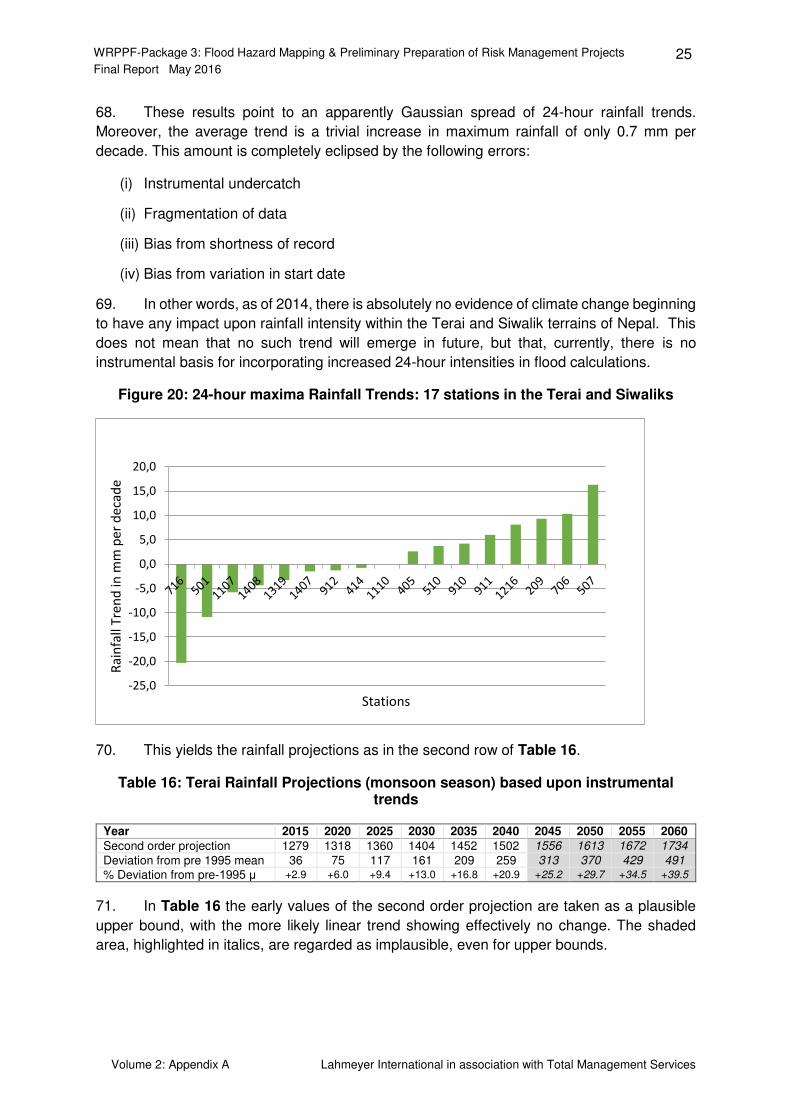
68. These results point to an apparently Gaussian spread of 24-hour rainfall trends.
Moreover, the average trend is a trivial increase in maximum rainfall of only 0.7 mm per
decade. This amount is completely eclipsed by the following errors:
(i) Instrumental undercatch
(ii) Fragmentation of data
(iii) Bias from shortness of record
(iv) Bias from variation in start date
69. In other words, as of 2014, there is absolutely no evidence of climate change beginning
to have any impact upon rainfall intensity within the Terai and Siwalik terrains of Nepal. This
does not mean that no such trend will emerge in future, but that, currently, there is no
instrumental basis for incorporating increased 24-hour intensities in flood calculations.
Figure 20: 24-hour maxima Rainfall Trends: 17 stations in the Terai and Siwaliks
70. This yields the rainfall projections as in the second row of Table 16.
Table 16: Terai Rainfall Projections (monsoon season) based upon instrumental trends
Year 2015 2020 2025 2030 2035 2040 2045 2050 2055 2060
Second order projection 1279 1318 1360 1404 1452 1502 1556 1613 1672 1734
Deviation from pre 1995 mean 36 75 117 161 209 259 313 370 429 491
% Deviation from pre-1995 μ +2.9 +6.0 +9.4 +13.0 +16.8 +20.9 +25.2 +29.7 +34.5 +39.5
71. In Table 16 the early values of the second order projection are taken as a plausible
upper bound, with the more likely linear trend showing effectively no change. The shaded
area, highlighted in italics, are regarded as implausible, even for upper bounds.
-25,0
-20,0
-15,0
-10,0
-5,0
0,0
5,0
10,0
15,0
20,0
Ra
infa
ll T
ren
d in
mm
pe
r d
eca
de
Stations
WRPPF-Package 3: Flood Hazard Mapping & Preliminary Preparation of Risk Management Projects 26 Final Report May 2016
Volume 2: Appendix A Lahmeyer International in association with Total Management Services
Inter-Study Comparison
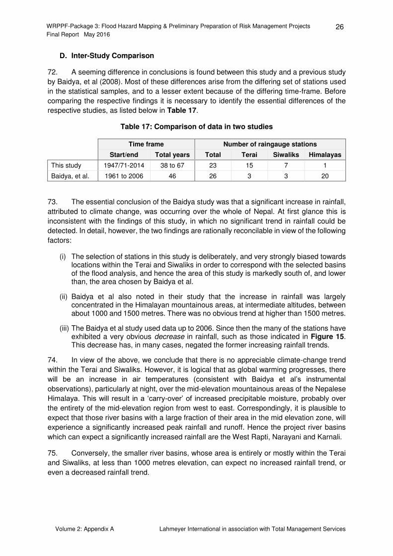
72. A seeming difference in conclusions is found between this study and a previous study
by Baidya, et al (2008). Most of these differences arise from the differing set of stations used
in the statistical samples, and to a lesser extent because of the differing time-frame. Before
comparing the respective findings it is necessary to identify the essential differences of the
respective studies, as listed below in Table 17.
Table 17: Comparison of data in two studies
Time frame Number of raingauge stations
Start/end Total years Total Terai Siwaliks Himalayas
This study 1947/71-2014 38 to 67 23 15 7 1
Baidya, et al. 1961 to 2006 46 26 3 3 20
73. The essential conclusion of the Baidya study was that a significant increase in rainfall,
attributed to climate change, was occurring over the whole of Nepal. At first glance this is
inconsistent with the findings of this study, in which no significant trend in rainfall could be
detected. In detail, however, the two findings are rationally reconcilable in view of the following
factors:
(i) The selection of stations in this study is deliberately, and very strongly biased towards locations within the Terai and Siwaliks in order to correspond with the selected basins of the flood analysis, and hence the area of this study is markedly south of, and lower than, the area chosen by Baidya et al.
(ii) Baidya et al also noted in their study that the increase in rainfall was largely concentrated in the Himalayan mountainous areas, at intermediate altitudes, between about 1000 and 1500 metres. There was no obvious trend at higher than 1500 metres.
(iii) The Baidya et al study used data up to 2006. Since then the many of the stations have exhibited a very obvious decrease in rainfall, such as those indicated in Figure 15. This decrease has, in many cases, negated the former increasing rainfall trends.
74. In view of the above, we conclude that there is no appreciable climate-change trend
within the Terai and Siwaliks. However, it is logical that as global warming progresses, there
will be an increase in air temperatures (consistent with Baidya et al’s instrumental observations), particularly at night, over the mid-elevation mountainous areas of the Nepalese
Himalaya. This will result in a ‘carry-over’ of increased precipitable moisture, probably over the entirety of the mid-elevation region from west to east. Correspondingly, it is plausible to
expect that those river basins with a large fraction of their area in the mid elevation zone, will
experience a significantly increased peak rainfall and runoff. Hence the project river basins
which can expect a significantly increased rainfall are the West Rapti, Narayani and Karnali.
75. Conversely, the smaller river basins, whose area is entirely or mostly within the Terai
and Siwaliks, at less than 1000 metres elevation, can expect no increased rainfall trend, or
even a decreased rainfall trend.
WRPPF-Package 3: Flood Hazard Mapping & Preliminary Preparation of Risk Management Projects 27 Final Report May 2016
Volume 2: Appendix A Lahmeyer International in association with Total Management Services
76. We very strongly emphasize that all such trends are on too small a scale to be
resolvable on any existing GCM or downscaled derivative, and hence support for these
conclusions should not be sought from modelling. On the contrary, improved resolution of the
differing rainfall trends will only be discernible from good-quality evidence-based instrumental
monitoring.
77. The question of ‘how much more rainfall’ can be attributed to climate change in the mid-elevation region is currently impossible to answer with any degree of assurance, in part
because the models are insufficiently precise, and in part because, in this study, the post-2006
mid-elevation station data were either too fragmented or not available.
78. The Baidya et al study indicated an increasing rainfall trend averaging about 2.3
mm.year-1, with 81 stations yielding a positive trend, and 14 basins yielding a negative trend.
This is equivalent to about a 5.0 % increase in rainfall, relative to 2006, by 2045 (mid-range of
the DHM modelling period). Taking the post-2006 station rainfall data into account shows that
this estimate is probably too high, in which case the DHM forward projection, of a 3.0% to
4.0% but may, perhaps, be taken as a conservative upper bound.
24-Hour Maximum Rainfall
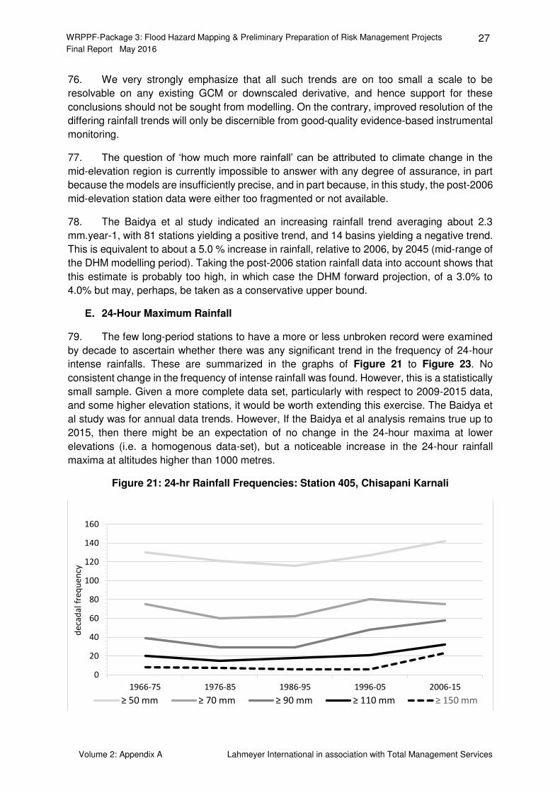
79. The few long-period stations to have a more or less unbroken record were examined
by decade to ascertain whether there was any significant trend in the frequency of 24-hour
intense rainfalls. These are summarized in the graphs of Figure 21 to Figure 23. No
consistent change in the frequency of intense rainfall was found. However, this is a statistically
small sample. Given a more complete data set, particularly with respect to 2009-2015 data,
and some higher elevation stations, it would be worth extending this exercise. The Baidya et
al study was for annual data trends. However, If the Baidya et al analysis remains true up to
2015, then there might be an expectation of no change in the 24-hour maxima at lower
elevations (i.e. a homogenous data-set), but a noticeable increase in the 24-hour rainfall
maxima at altitudes higher than 1000 metres.
Figure 21: 24-hr Rainfall Frequencies: Station 405, Chisapani Karnali
0
20
40
60
80
100
120
140
160
1966-75 1976-85 1986-95 1996-05 2006-15
de
cad
al
fre
qu
en
cy
≥ 5 mm ≥ 7 mm ≥ 9 mm ≥ mm ≥ 5 mm
WRPPF-Package 3: Flood Hazard Mapping & Preliminary Preparation of Risk Management Projects 28 Final Report May 2016
Volume 2: Appendix A Lahmeyer International in association with Total Management Services
Figure 22: 24-hr Rainfall Frequencies: Station 911, Parwanipur
Figure 23: 24-hr Rainfall Frequencies: Station 1216, Siraha
0
20
40
60
80
100
120
1966-75 1976-85 1986-95 1996-05 2006-15
de
cad
al
fre
qu
en
cy
≥ 5 mm ≥ 7 mm ≥ 9 mm ≥ mm ≥ 5 mm
0
10
20
30
40
50
60
70
80
90
1946-55 1956-65 1966-75 1976-85 1986-95 1996-05 2006-15
de
cad
al f
req
ue
ncy
≥ 5 mm ≥ 7 mm ≥ 9 mm ≥ mm ≥ 5 mm
WRPPF-Package 3: Flood Hazard Mapping & Preliminary Preparation of Risk Management Projects 29 Final Report May 2016
Volume 2: Appendix A Lahmeyer International in association with Total Management Services
III. RAINFALL INPUT FOR BASIN-RUNOFF MODELLING
80. It is evident from initial modelling results that the conventional distribution of
representative areas using ‘Thiessen polygons’ may be appropriate for relatively uniform-
rainfall areas, such as catchments largely or wholly within the Terai, but is wholly inadequate
to represent rainfall within mountainous terrains such as the Siwaliks and Lower Himalayas.
There are three reasons why the rain-data within the Siwaliks are skewed towards lower than
actual values:
(i) In most river basins the logistics of instrumental maintenance result in a preponderance of raingauges in valleys and low-gradient areas, where markedly lesser rainfall is experienced.
(ii) The raingauge network density is higher at lower elevations than in the catchment boundary areas.
(iii) The winds are stronger at higher elevations, and particularly around watershed boundaries (turbulent vortices), resulting in a greater instrumental under-catch.
81. Accordingly, some attempt at a more realistic rainfall input to the catchment models
was required. As already indicated in Figure 2, the rainfall altitude relationship is poorly
quantified, and lacks calibrated process studies to characterise the various physiographic
influences. An attempt to optimise a rainfall-altitude relationship using 3rd and 4th order
equations proved unsatisfactory. Therefore, we have adopted very approximate empirical
growth factors for different altitude ranges, relative to the rainfall at 1000 metres. These are
given in Table 18. In practice we regard the growth factors of ‘B’ and ‘C’ (3rd and 4th lines of
Table 18) as yielding plausible lower and upper bounds, respectively.
Table 18: Adopted mean rainfall-altitude relationships, normalised with respect to the rainfall at 1000 metres.
Altitude, (metres): 1000 1250-1750 1750-2250 >2250
A: 4th order regression 1 1.08 1.14 1.05
B: moderate R-A gradient 1 1.05 1.25 1.03
C: steep R-A gradient 1 1.3 1.4 1
Mean of B and C 1 1.18 1.33 1.02
82. Table 18 is for the seasonal or annual rainfall-altitude relationship. For flood analytical
purposes it is more useful to consider the 24-hour rainfall-altitude relationship. Even more
useful would be even shorter period rainfall time steps, but these data will not become
available until the current and proposed pluviometers data have built up a sufficiently long
time-series to be useful.
83. The 24-hour maxima have been plotted in Figure 15 to Figure 18.
84. We acknowledge that these factors constitute a crude approach to correcting the input
rainfall for modelling. This is regarded as provisional pending a more scientifically robust
method of assessment. In respect of the latter, the requirements for flood estimation, water
resources evaluation and hydroelectric planning, all underscore the need for detailed
WRPPF-Package 3: Flood Hazard Mapping & Preliminary Preparation of Risk Management Projects 30 Final Report May 2016
Volume 2: Appendix A Lahmeyer International in association with Total Management Services
hydrologic studies. The requirement, which is far beyond the scope of this project, is for an
intensively instrumented experimental catchment, and data collection for at least a decade
with a view to developing a multi-variate expression of the form: �� = . � 2 + . � + . � + . � + . + .
85. Where RF is the rainfall, a, b, c, d, e and f are empirical constants, Alt is the altitude
assuming a second order relationship at least up to 2000 metres, Tr is the quantified trend
parallel to the mountain front, Asp is the quantified aspect, Bar is the quantified barrier effect,
and Car is the quantified ‘carry-over’ effect.
86. We emphasize that whilst the development of such an expression is entirely an office
activity, the data required will require a major and sustained input of field-work. There are no
short cuts, and this data cannot be measured by remote sensing. This is beyond current
institutional capabilities, and will require donor input.
87. It has been suggested that the rainfall in mountainous areas be estimated upon the
basis of isohyetal mapping. Apparent isohyetal maps already exist, (ICIMOD, 1996; Dhar &
Nandargi, 2006) but we strongly emphasize that such maps are currently ill-founded and highly
misleading for the following reasons:
(i) As already discussed, the raingauge network upon which the isohyetal maps are based, is sub-optimal.
(ii) The isohyets are generated by a contouring package which takes no account of the all- important physiographic controls.
(iii) The raingauge data is treated as a homogeneous subset of the greater set of homogeneous data. This gives rise to such anomalies as concentric isohyets distributed around point-rainfall maxima and minima. These are ‘ghost contours’ which are purely artefacts of the contouring algorithm, and bear no relation to reality.
88. It will be possible to generate a realistic isohyetal map if, and only if, the multi-variate
approach is adopted. In the interim, the provisional (and inaccurate) isohyetal maps could, in
principle, be greatly improved by combining the data with precipitation radar reflection data.
WRPPF-Package 3: Flood Hazard Mapping & Preliminary Preparation of Risk Management Projects 31 Final Report May 2016
Volume 2: Appendix A Lahmeyer International in association with Total Management Services
IV. CONCLUSIONS
89. There is a general perception that climate change will result in increasing rainfall over
time, whether considered as increased frequency of 24-hour extremes, monsoonal or annual.
In this study we conclude that the changing rainfall distribution is more complex. The main
conclusions are as follows.
(i) The evidence-based instrumental record for the Terai and Siwaliks region, up to 2014, indicated neither increased frequency of high rainfall events, nor any increase in overall total rainfall (monsoon or annual). Local positive rainfall anomalies are almost perfectly balanced by an equal number and intensity of negative rainfall anomalies.
(ii) On the basis of the above there are no climate-change grounds for increasing the model rainfall inputs for those basins which are entirely within the Terai or lower Siwalik areas.
(iii) Climate models for those river basins entirely within the Terai and Siwaliks, also indicate a net decrease in rainfall over time. This is true irrespective of the cluster of models used, for all scenarios, for all forecasted time periods, and regardless of west-east location along the mountain front.
(iv) For basins with a substantial area within the mid-altitude range, north of the Siwaliks, and typically up to about 1500 metres (maybe up to 2000 metres in some places) there is a dramatically different climate change outcome, in which the rainfall greatly increases over time. We estimate this increase to vary between 15% and 62%, (see Table 10).
(v) We cannot prove, but strongly suspect, that a single causal mechanism of increasing mean air temperatures, accounts for both of the above trends. Higher temperatures along the Terai will somewhat suppress precipitation at lower elevations, but will carry over a greatly increased precipitable moisture to higher, more northerly parts of Nepal, including some of the upper basins of this flood study. This is consistent with the findings of this study, that of Baidya et al (2006), and with the CMIP5 modelling results (both the means and medians of 16 models).
(vi) In view of the above we recommend that climate-change weightings, as specified in Table 10 (as upper and lower bounds), be applied to the model rainfall inputs for the basins Karnali, Narayani, West Rapti, and Kankai for the fraction of the basins that is north of the Siwaliks.
(vii) Quite apart from climate change trends there is a further adjustment that is requires in the Karnali, Narayani, West Rapti and Kankai basins to account for the rainfall increase with altitude up to about 1500 metres (maybe up to 2000 metres). These adjustment factors, listed in Table 18, are somewhat crude and in need of improvement through rainfall-physiography process studies. Despite the need for caution in this relationship, we believe that elevation-range adjustments will be a marked improvement on the previous ‘Thiessen polygon’ methodology.
(viii) Within the Terai and Siwaliks the elevation adjustment is likely to be small, in which case the rainfall input may continue to be estimated on the basis of Thiessen polygons.
WRPPF-Package 3: Flood Hazard Mapping & Preliminary Preparation of Risk Management Projects 32 Final Report May 2016
Volume 2: Appendix A Lahmeyer International in association with Total Management Services
V. REFERENCES
Baidya S, Shrestha M.L, and Sheikh M.M., (2008). Trends in Daily Climatic Extremes of
Temperature and Precipitation in Nepal. Journ. Hydrol. and Meteorology. 5, (1), 38-51.
Bin Wang (2006). The Asian Monsoon. 791pp. Springer Verlag Chalise S.R., Shrestha M.L, et al (1996).Climate and Hydrological Atlas of Nepal. ICIMOD.
262pp. Dhar O.N and Nandargi S (2006). Areas of heavy precipitation in the Nepalese Himalayas.
Weather, 60, (12), 354-356. Lopez M/G. et al, (2015). Location and Density of Rain Gauges for the Estimation of Spatial
Varying Precipitation. Geografiska Annaler: Ser. A Physical Geography. 97, (1) 167-179.
Marahata S., Dangol B.S., and Gurung G.B., for ‘Practical Action Nepal Office’ (2009).
Temporal and Spatial Variability of Climate Change over Nepal (1976 - 2005). 76pp. https://practicalaction.org/file/region_nepal/ClimateChange1976-2005.pdf
Shrestha, D., Singh P., and Nakamura K (2012). Spatiotemporal variation of rainfall over the
central Himalayan region revealed by TRMM Precipitation Radar. Jour. Geophys. Res. 117, D22106, doi:10.1029/2012JD018140, (14pp).
Singh P and Singh V.P, (2001). Snow and Glacier Hydrology. Kluer Academic. 742pp. Timalsina P. (2014). Development of Intensity Duration Frequency Relationship of Rainfall
extremes and Regionalization. M.Sc. thesis, 99pp; Tribhuvan University, Institute Of Engineering.
Volkman TH.M. et al (2010). Multicriteria design of rain gauge networks for flash flood
prediction in semiarid catchments with complex terrain. Water Resources Research 46, W11554, doi:10.1029/2010WR009145, 16pp.
Westra S, Alexander L.V. and Zwiers F.W. (2013) Global Increasing Trends in Annual
Maximum Daily Precipitation. http://envsci.rutgers.edu/~toine379/extremeprecip/papers/westra_et_al_2013.pdf
WRPPF-Package 3: Flood Hazard Mapping & Preliminary Preparation of Risk Management Projects 33 Final Report May 2016
Volume 2: Appendix A Lahmeyer International in association with Total Management Services
ANNEX 1: MONTHLY RAINFALL SUMMARIES
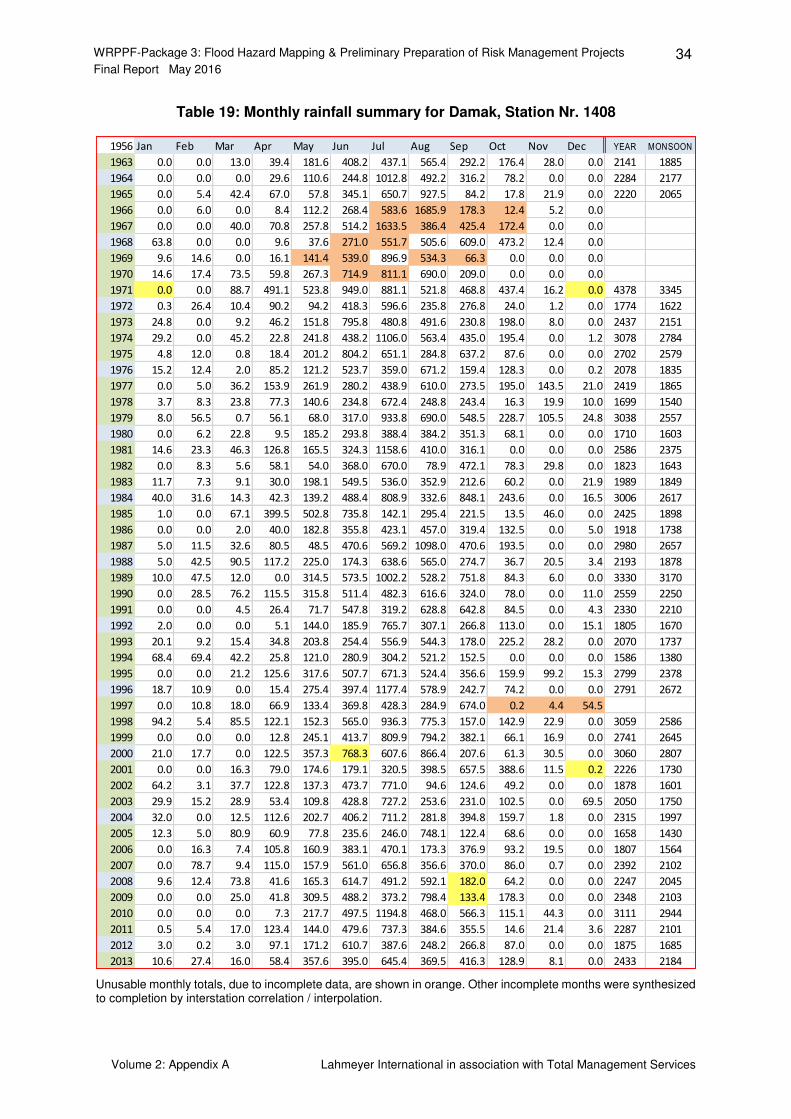
WRPPF-Package 3: Flood Hazard Mapping & Preliminary Preparation of Risk Management Projects 34 Final Report May 2016
Volume 2: Appendix A Lahmeyer International in association with Total Management Services
Table 19: Monthly rainfall summary for Damak, Station Nr. 1408
Unusable monthly totals, due to incomplete data, are shown in orange. Other incomplete months were synthesized to completion by interstation correlation / interpolation.
1956 Jan Feb Mar Apr May Jun Jul Aug Sep Oct Nov Dec YEAR MONSOON
1963 0.0 0.0 13.0 39.4 181.6 408.2 437.1 565.4 292.2 176.4 28.0 0.0 2141 1885
1964 0.0 0.0 0.0 29.6 110.6 244.8 1012.8 492.2 316.2 78.2 0.0 0.0 2284 2177
1965 0.0 5.4 42.4 67.0 57.8 345.1 650.7 927.5 84.2 17.8 21.9 0.0 2220 2065
1966 0.0 6.0 0.0 8.4 112.2 268.4 583.6 1685.9 178.3 12.4 5.2 0.0
1967 0.0 0.0 40.0 70.8 257.8 514.2 1633.5 386.4 425.4 172.4 0.0 0.0
1968 63.8 0.0 0.0 9.6 37.6 271.0 551.7 505.6 609.0 473.2 12.4 0.0
1969 9.6 14.6 0.0 16.1 141.4 539.0 896.9 534.3 66.3 0.0 0.0 0.0
1970 14.6 17.4 73.5 59.8 267.3 714.9 811.1 690.0 209.0 0.0 0.0 0.0
1971 0.0 0.0 88.7 491.1 523.8 949.0 881.1 521.8 468.8 437.4 16.2 0.0 4378 3345
1972 0.3 26.4 10.4 90.2 94.2 418.3 596.6 235.8 276.8 24.0 1.2 0.0 1774 1622
1973 24.8 0.0 9.2 46.2 151.8 795.8 480.8 491.6 230.8 198.0 8.0 0.0 2437 2151
1974 29.2 0.0 45.2 22.8 241.8 438.2 1106.0 563.4 435.0 195.4 0.0 1.2 3078 2784
1975 4.8 12.0 0.8 18.4 201.2 804.2 651.1 284.8 637.2 87.6 0.0 0.0 2702 2579
1976 15.2 12.4 2.0 85.2 121.2 523.7 359.0 671.2 159.4 128.3 0.0 0.2 2078 1835
1977 0.0 5.0 36.2 153.9 261.9 280.2 438.9 610.0 273.5 195.0 143.5 21.0 2419 1865
1978 3.7 8.3 23.8 77.3 140.6 234.8 672.4 248.8 243.4 16.3 19.9 10.0 1699 1540
1979 8.0 56.5 0.7 56.1 68.0 317.0 933.8 690.0 548.5 228.7 105.5 24.8 3038 2557
1980 0.0 6.2 22.8 9.5 185.2 293.8 388.4 384.2 351.3 68.1 0.0 0.0 1710 1603
1981 14.6 23.3 46.3 126.8 165.5 324.3 1158.6 410.0 316.1 0.0 0.0 0.0 2586 2375
1982 0.0 8.3 5.6 58.1 54.0 368.0 670.0 78.9 472.1 78.3 29.8 0.0 1823 1643
1983 11.7 7.3 9.1 30.0 198.1 549.5 536.0 352.9 212.6 60.2 0.0 21.9 1989 1849
1984 40.0 31.6 14.3 42.3 139.2 488.4 808.9 332.6 848.1 243.6 0.0 16.5 3006 2617
1985 1.0 0.0 67.1 399.5 502.8 735.8 142.1 295.4 221.5 13.5 46.0 0.0 2425 1898
1986 0.0 0.0 2.0 40.0 182.8 355.8 423.1 457.0 319.4 132.5 0.0 5.0 1918 1738
1987 5.0 11.5 32.6 80.5 48.5 470.6 569.2 1098.0 470.6 193.5 0.0 0.0 2980 2657
1988 5.0 42.5 90.5 117.2 225.0 174.3 638.6 565.0 274.7 36.7 20.5 3.4 2193 1878
1989 10.0 47.5 12.0 0.0 314.5 573.5 1002.2 528.2 751.8 84.3 6.0 0.0 3330 3170
1990 0.0 28.5 76.2 115.5 315.8 511.4 482.3 616.6 324.0 78.0 0.0 11.0 2559 2250
1991 0.0 0.0 4.5 26.4 71.7 547.8 319.2 628.8 642.8 84.5 0.0 4.3 2330 2210
1992 2.0 0.0 0.0 5.1 144.0 185.9 765.7 307.1 266.8 113.0 0.0 15.1 1805 1670
1993 20.1 9.2 15.4 34.8 203.8 254.4 556.9 544.3 178.0 225.2 28.2 0.0 2070 1737
1994 68.4 69.4 42.2 25.8 121.0 280.9 304.2 521.2 152.5 0.0 0.0 0.0 1586 1380
1995 0.0 0.0 21.2 125.6 317.6 507.7 671.3 524.4 356.6 159.9 99.2 15.3 2799 2378
1996 18.7 10.9 0.0 15.4 275.4 397.4 1177.4 578.9 242.7 74.2 0.0 0.0 2791 2672
1997 0.0 10.8 18.0 66.9 133.4 369.8 428.3 284.9 674.0 0.2 4.4 54.5
1998 94.2 5.4 85.5 122.1 152.3 565.0 936.3 775.3 157.0 142.9 22.9 0.0 3059 2586
1999 0.0 0.0 0.0 12.8 245.1 413.7 809.9 794.2 382.1 66.1 16.9 0.0 2741 2645
2000 21.0 17.7 0.0 122.5 357.3 768.3 607.6 866.4 207.6 61.3 30.5 0.0 3060 2807
2001 0.0 0.0 16.3 79.0 174.6 179.1 320.5 398.5 657.5 388.6 11.5 0.2 2226 1730
2002 64.2 3.1 37.7 122.8 137.3 473.7 771.0 94.6 124.6 49.2 0.0 0.0 1878 1601
2003 29.9 15.2 28.9 53.4 109.8 428.8 727.2 253.6 231.0 102.5 0.0 69.5 2050 1750
2004 32.0 0.0 12.5 112.6 202.7 406.2 711.2 281.8 394.8 159.7 1.8 0.0 2315 1997
2005 12.3 5.0 80.9 60.9 77.8 235.6 246.0 748.1 122.4 68.6 0.0 0.0 1658 1430
2006 0.0 16.3 7.4 105.8 160.9 383.1 470.1 173.3 376.9 93.2 19.5 0.0 1807 1564
2007 0.0 78.7 9.4 115.0 157.9 561.0 656.8 356.6 370.0 86.0 0.7 0.0 2392 2102
2008 9.6 12.4 73.8 41.6 165.3 614.7 491.2 592.1 182.0 64.2 0.0 0.0 2247 2045
2009 0.0 0.0 25.0 41.8 309.5 488.2 373.2 798.4 133.4 178.3 0.0 0.0 2348 2103
2010 0.0 0.0 0.0 7.3 217.7 497.5 1194.8 468.0 566.3 115.1 44.3 0.0 3111 2944
2011 0.5 5.4 17.0 123.4 144.0 479.6 737.3 384.6 355.5 14.6 21.4 3.6 2287 2101
2012 3.0 0.2 3.0 97.1 171.2 610.7 387.6 248.2 266.8 87.0 0.0 0.0 1875 1685
2013 10.6 27.4 16.0 58.4 357.6 395.0 645.4 369.5 416.3 128.9 8.1 0.0 2433 2184

WRPPF-Package 3: Flood Hazard Mapping & Preliminary Preparation of Risk Management Projects 35 Final Report May 2016
Volume 2: Appendix A Lahmeyer International in association with Total Management Services
Table 20: Monthly rainfall summary for Parwanipur, Station Nr. 911
Unusable monthly totals, due to incomplete data, are shown in orange. Other incomplete months were synthesized to completion by interstation correlation / interpolation.
Jan Feb Mar Apr May Jun Jul Aug Sep Oct Nov Dec YEAR Mon'n
1967 6 15.8 20 64.2 152.5 231.6 668.2 137.2 311.6 189.5 8 4.5 1809 1501
1968 9.5 18 3.3 20.4 28.5 296.6 604.6 219.7 282.6 34 10.5 22.7 1550 1432
1969 0 1.1 16 0.5 124 273.5 406.1 215.7 103.1 20 0 1.6 1162 1122
1970 51.5 6 18 91 170.5 272.3 685.3 317.5 426 0 14 0 2052 1872
1971 11.5 0.7 50.5 68 63 306.5 361.4 87.5 151 21 9 7.6 1138 969
1972 30.5 0 1 47 117.5 89.5 432.3 243.9 52.6 56.2 0 25.8 1096 936
1973 27.5 22 5.5 48.8 108.1 652.5 565.4 133.3 332.9 9 0 8.3 1913 1792
1974 6 2 6.3 4.4 72.2 333.8 481.7 430.8 612.5 118.4 5 36.6 2110 1931
1975 2 32.5 0 23.5 62 398.7 368.5 487.2 308.3 96.3 11.7 65 1856 1625
1976 1 8.8 13.3 83.4 42.7 125.7 824.3 582.9 132.9 139.4 0 4.5 1959 1709
1977 0 22.5 51.4 54 174.5 221.3 454.3 519.7 309.9 44.2 0 40 1892 1680
1978 0.5 21.2 18.1 0 131.1 157.1 491.1 171.3 192.4 33.5 2.2 5.3 1224 1143
1979 0 33.2 11 96.6 186.4 150.5 335.7 119.8 272.1 34.3 0 3.4 1243 1065
1980 33.5 1.3 16 8 99 512.1 201.7 598.4 227.1 23.5 0 17.2 1738 1638
1981 5 12.7 0 17.7 119.6 100.9 383.1 202.3 77.8 113.8 5.6 0 1039 884
1982 3.2 5.9 40.7 77.4 77.5 261.1 616.9 536.7 147.2 15.7 5.6 0 1788 1639
1983 41 24.5 18.2 4.7 82.6 128.4 246.9 226.9 326.1 40.5 0 0 1140 1011
1984 4.5 33 24.3 0 19.6 311.6 207.6 494 187.8 0 47.9 26 1356 1221
1985 23.3 0 31.2 21.2 190.4 397.3 271.1 182.1 102.2 0 0 20.3 1239 1143
1986 20.3 0 3.6 50.2 109.7 401.6 192.6 194.9 230.8 0 0 90.7 1294 1130
1987 13 0 54.1 26.6 99.6 175.8 972 535.6 291 57.8 20.3 0 2246 2074
1988 0 0 0 18.3 93.5 501.5 362.9 445 116.7 85.8 0 0 1624 1520
1989 17 6 0 87.6 259.5 297.9 588.9 358.2 131.7 0 0 0 1747 1636
1990 0 0 8.7 30.5 275.8 284.7 426 397.5 361.4 114.5 0 0 1899 1745
1991 50.2 31.6 2 31.2 195 323.8 630.6 143.2 352.3 17.8 19 19.2 1816 1645
1992 39.5 25 79.5 21.02 0.29 601.6 51.19 318 271.6 63.4 0 1 1472 1243
1993 15.8 0 0 98.2 110.7 612 557 158.4 214.1 75.4 4.6 0 1846 1652
1994 20.9 6.3 14.7 11.5 76.6 101 381.5 814.3 47.7 64.3 0 0 1539 1421
1995 0 0 6.9 79 121.4 333.4 358.3 118.8 261 124.6 0 27.9 1431 1193
1996 0 65.5 14 2 63 349.8 1065 487.8 283.2 59.2 1 0 2390 2249
1997 1.8 0 25.5 32.3 85.7 369.6 578.2 421.1 151.4 16.1 0 0 1682 1606
1998 0 0 0 7.8 120.2 137.8 402.5 694.4 55.3 41.3 0 12.6 1472 1410
1999 0 3.6 0 29.3 102.3 194.9 247.4 295.9 144.5 182.2 0 1.4 1202 985
2000 1.7 21.5 30.5 92.9 141 131.5 756.2 316.5 187.7 5.1 16.31 15.1 1716 1533
2001 0 7.6 5 40.2 14.8 224.8 0 215.3 0 1.2 0 0 509 455
2002 3.4 21.7 9 42.7 192.3 432.9 263.2 311.2 111.5 213.9 0 0 1602 1311
2003 11 18.5 0 1 263.5 228.5 255.8 464 211.6 130.1 0 7.81
2010 0.01 3.6 0 29.3 102.3 161.9 280.4 294.3 146.1 182.2 0 0 1200 985
2011 3.1 21.5 30.5 38.51 180.4 0 851.1 353.1 187.7 5.1 16.31 0
2012 15.11 7.61 5.01 40.21 14.8 214.8 0 194.3 0 1.21 0 0
2013 3.4 21.71 9 40.71 186.8 417.6 277 311.2 111.5 213.9 0 0 1593 1304
2014 11 18.2 0.3 0 264.5 227.5 255.8 464 210.8 130.9 0 7.81 1591 1423
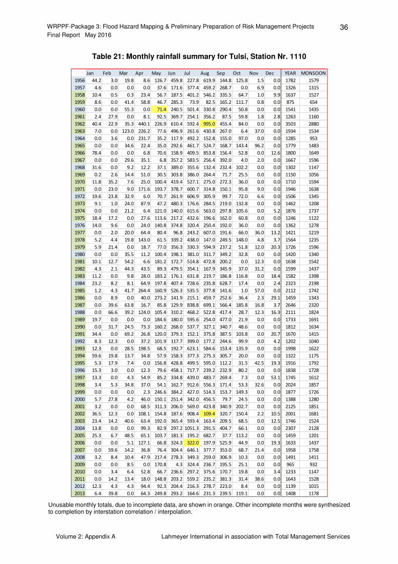
WRPPF-Package 3: Flood Hazard Mapping & Preliminary Preparation of Risk Management Projects 36 Final Report May 2016
Volume 2: Appendix A Lahmeyer International in association with Total Management Services
Table 21: Monthly rainfall summary for Tulsi, Station Nr. 1110
Unusable monthly totals, due to incomplete data, are shown in orange. Other incomplete months were synthesized to completion by interstation correlation / interpolation.
1956 Jan Feb Mar Apr May Jun Jul Aug Sep Oct Nov Dec YEAR MONSOON
1956 44.2 3.0 19.8 8.6 126.7 459.8 227.8 619.9 144.8 125.8 1.5 0.0 1782 1579
1957 4.6 0.0 0.0 0.0 37.6 171.6 377.4 459.2 268.7 0.0 6.9 0.0 1326 1315
1958 10.4 0.5 0.3 23.4 56.7 187.5 401.2 546.2 335.5 64.7 1.0 9.9 1637 1527
1959 8.6 0.0 41.4 58.8 46.7 285.3 73.9 82.5 165.2 111.7 0.8 0.0 875 654
1960 0.0 0.0 55.3 0.0 71.4 240.5 501.4 330.8 290.4 50.8 0.0 0.0 1541 1435
1961 2.4 27.9 0.0 8.1 92.5 369.7 254.1 356.2 87.5 59.8 1.8 2.8 1263 1160
1962 40.4 22.9 35.3 440.1 226.9 610.4 592.4 995.0 455.4 84.0 0.0 0.0 3503 2880
1963 7.0 0.0 123.0 226.2 77.6 496.9 261.6 430.8 267.0 6.4 37.0 0.0 1934 1534
1964 0.0 3.6 0.0 231.7 35.2 117.9 492.2 152.8 155.0 97.0 0.0 0.0 1285 953
1965 0.0 0.0 34.6 22.4 35.0 292.6 461.7 524.7 168.7 143.4 96.2 0.0 1779 1483
1966 78.4 0.0 0.0 6.8 70.6 158.9 409.5 853.8 156.4 52.8 0.0 12.6 1800 1649
1967 0.0 0.0 29.6 35.1 6.8 357.2 583.5 256.4 392.0 4.0 2.0 0.0 1667 1596
1968 31.6 0.0 9.2 12.2 37.1 389.0 355.6 132.4 232.4 102.2 0.0 0.0 1302 1147
1969 0.2 2.6 14.4 51.0 30.5 303.8 386.0 264.4 71.7 25.5 0.0 0.0 1150 1056
1970 11.8 35.2 7.6 25.0 100.4 419.4 527.1 275.0 272.3 36.0 0.0 0.0 1710 1594
1971 0.0 23.0 9.0 171.6 193.7 378.7 600.7 314.8 150.1 95.8 9.0 0.0 1946 1638
1972 19.6 23.8 32.9 6.0 70.7 261.9 606.9 305.9 99.7 72.0 6.6 0.0 1506 1345
1973 9.1 1.0 24.0 87.9 47.2 480.3 176.6 284.5 219.0 132.8 0.0 0.0 1462 1208
1974 0.0 0.0 21.2 6.4 121.0 140.0 615.6 563.0 297.8 105.6 0.0 5.2 1876 1737
1975 18.4 17.2 0.0 27.6 113.6 217.2 432.6 196.6 162.0 60.8 0.0 0.0 1246 1122
1976 14.0 9.6 0.0 24.0 140.8 374.8 320.4 250.4 192.0 36.0 0.0 0.0 1362 1278
1977 0.0 2.0 20.0 64.4 80.4 96.8 243.2 607.0 191.6 66.0 36.0 13.2 1421 1219
1978 5.2 4.4 19.8 143.0 61.5 339.2 438.0 147.0 249.5 148.0 4.8 3.7 1564 1235
1979 5.9 21.4 0.0 18.7 77.0 356.3 330.3 594.9 237.2 51.8 12.0 20.3 1726 1596
1980 0.0 0.0 35.5 11.2 100.4 198.1 381.0 311.7 349.2 32.8 0.0 0.0 1420 1340
1981 10.1 12.7 54.2 6.6 181.2 172.7 514.8 472.8 200.2 0.0 12.3 0.0 1638 1542
1982 4.3 2.1 44.3 43.5 89.3 479.5 354.1 167.9 345.9 37.0 31.2 0.0 1599 1437
1983 11.2 0.0 9.8 28.0 183.2 176.1 631.8 219.7 186.8 116.8 0.0 18.4 1582 1398
1984 23.2 8.2 8.1 64.9 197.8 407.4 728.6 235.8 628.7 17.4 0.0 2.4 2323 2198
1985 1.2 4.3 41.7 264.4 160.9 526.3 535.5 377.8 141.6 1.0 57.0 0.0 2112 1742
1986 0.0 8.9 0.0 40.0 273.2 141.9 215.1 459.7 252.6 36.4 2.3 29.1 1459 1343
1987 0.0 39.6 63.8 16.7 85.8 129.9 838.8 699.1 566.4 185.8 16.8 3.7 2646 2320
1988 0.0 66.6 39.2 124.0 105.4 310.2 468.2 522.8 417.4 28.7 12.3 16.3 2111 1824
1989 19.7 0.0 0.0 0.0 184.6 180.0 595.6 254.0 477.0 21.9 0.0 0.0 1733 1691
1990 0.0 31.7 24.5 73.3 160.2 268.0 537.7 327.1 340.7 48.6 0.0 0.0 1812 1634
1991 34.4 0.0 69.2 26.8 120.0 379.3 152.1 375.8 387.5 103.8 0.0 20.7 1670 1415
1992 8.3 12.3 0.0 37.2 101.9 117.7 399.0 177.2 244.6 99.9 0.0 4.2 1202 1040
1993 12.3 0.0 28.5 198.5 68.5 192.7 623.1 584.6 153.4 135.9 0.0 0.0 1998 1622
1994 59.6 19.8 13.7 34.8 57.9 158.3 377.3 275.3 305.7 20.0 0.0 0.0 1322 1175
1995 5.3 17.9 7.4 0.0 156.8 428.8 499.5 595.0 112.2 31.5 42.5 19.3 1916 1792
1996 15.3 3.0 0.0 12.3 79.6 458.1 717.7 239.2 232.9 80.2 0.0 0.0 1838 1728
1997 13.3 0.0 4.3 54.9 85.2 334.8 439.0 483.7 269.4 7.3 0.0 53.1 1745 1612
1998 3.4 5.3 34.8 37.0 54.1 162.7 912.6 556.3 171.4 53.3 32.6 0.0 2024 1857
1999 0.0 0.0 0.0 2.3 246.6 384.2 427.0 514.3 153.7 149.3 0.0 0.0 1877 1726
2000 5.7 27.8 4.2 46.0 150.1 251.4 342.0 456.5 79.7 24.5 0.0 0.0 1388 1280
2001 3.2 0.0 0.0 68.5 311.3 206.0 569.0 423.8 340.9 202.7 0.0 0.0 2125 1851
2002 36.5 12.3 0.0 108.1 154.8 187.6 908.4 109.4 320.7 150.4 2.2 10.5 2001 1681
2003 23.4 14.2 40.6 63.4 192.0 365.4 593.4 163.4 209.5 68.5 0.0 12.5 1746 1524
2004 13.8 0.0 0.0 99.3 82.9 297.2 1051.3 291.5 404.7 66.1 0.0 0.0 2307 2128
2005 25.3 6.7 48.5 65.1 103.7 181.3 195.2 682.7 37.7 113.2 0.0 0.0 1459 1201
2006 0.0 0.0 5.1 127.1 66.8 324.3 322.0 197.9 525.9 44.9 0.0 19.3 1633 1437
2007 0.0 59.6 14.2 36.8 76.4 304.4 646.1 377.7 353.0 68.7 21.4 0.0 1958 1758
2008 3.2 8.4 10.4 47.9 217.4 278.3 349.3 259.0 306.9 10.3 0.0 0.0 1491 1411
2009 0.0 0.0 8.5 0.0 170.8 4.3 324.4 236.7 195.5 25.1 0.0 0.0 965 932
2010 0.0 3.4 6.4 52.8 66.7 236.6 297.2 375.6 170.7 19.8 0.0 3.4 1233 1147
2011 0.0 14.2 13.4 18.0 148.8 203.2 559.2 235.2 381.3 31.4 38.6 0.0 1643 1528
2012 12.3 4.3 4.3 94.4 92.3 204.4 216.3 278.7 223.0 8.4 0.0 0.0 1139 1015
2013 6.4 39.8 0.0 64.3 249.8 293.2 164.6 231.3 239.5 119.1 0.0 0.0 1408 1178
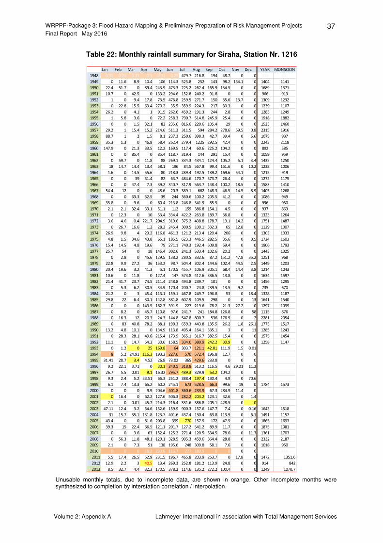
WRPPF-Package 3: Flood Hazard Mapping & Preliminary Preparation of Risk Management Projects 37 Final Report May 2016
Volume 2: Appendix A Lahmeyer International in association with Total Management Services
Table 22: Monthly rainfall summary for Siraha, Station Nr. 1216
Unusable monthly totals, due to incomplete data, are shown in orange. Other incomplete months were synthesized to completion by interstation correlation / interpolation.
Jan Feb Mar Apr May Jun Jul Aug Sep Oct Nov Dec YEAR MONSOON
1948 0.31 0.29 0.31 0.3 0.31 0.29 479.7 216.8 194 48.7 0 0 939 891
1949 0 11.6 8.9 10.4 106 114.3 525.8 252 143 98.2 134.1 0 1404 1141
1950 22.4 51.7 0 89.4 243.9 473.3 225.2 262.4 165.9 154.5 0 0 1689 1371
1951 10.7 0 42.5 0 133.2 294.6 152.8 240.2 91.8 0 0 0 966 913
1952 1 0 9.4 17.8 73.5 476.8 259.5 271.7 150 35.6 13.7 0 1309 1232
1953 0 22.8 15.5 63.4 270.2 35.5 359.9 224.3 217 30.3 0 0 1239 1107
1954 26.2 0 4.1 1 91.5 262.6 459.2 191.3 244 2.8 0 0 1283 1249
1955 1 5.8 3.6 0 72.2 258.3 790.7 514.8 245.9 25.4 0 0 1918 1882
1956 0 0 1.5 32.1 82 235.6 816.6 220.6 105.4 29 0 0 1523 1460
1957 29.2 1 15.4 15.2 214.6 511.3 311.5 594 284.2 278.6 59.5 0.8 2315 1916
1958 88.7 1 2 1.5 8.1 237.3 250.6 398.3 42.7 39.4 0 5.6 1075 937
1959 35.3 1.3 0 46.8 58.4 262.4 279.4 1225 292.5 42.4 0 0 2243 2118
1960 147.9 0 21.3 33.5 12.2 169.5 117.4 60.6 225.2 104.2 0 0 892 585
1961 0 0 85.4 0 85.4 118.7 319.4 144 291 15.4 0 0 1059 959
1962 0 59.7 0 11.8 88 269.1 334.3 434.1 124.4 105.2 5.1 3.4 1435 1250
1963 18 14.7 14.4 13.4 58.1 196 84.5 567.8 99.4 161.6 0 10.2 1238 1006
1964 1.6 0 14.5 55.6 80 218.3 289.4 192.5 139.2 169.6 54.1 0 1215 919
1965 0 0 39 31.4 82 63.7 484.6 170.7 373.7 26.4 0 0 1272 1175
1966 0 0 47.4 7.3 39.2 340.7 317.9 563.7 148.4 100.2 18.5 0 1583 1410
1967 54.4 12 0 0 48.6 20.3 389.1 662 148.3 46.5 14.5 8.9 1405 1268
1968 0 0 63.3 32.5 39 244 360.6 100.2 205.5 41.2 0 0 1086 949
1969 35.8 0 9.6 0 60.4 213.8 248.8 341.9 85.5 0 0 0 996 950
1970 2.1 2.1 32.4 33.1 51.1 112 159 386.8 154.1 4.5 0 0 937 863
1971 0 12.3 0 10 53.4 334.4 422.2 263.8 189.7 36.8 0 0 1323 1264
1972 3.6 4.6 0.4 221.7 204.9 319.6 375.2 408.8 178.7 19.1 14.2 0 1751 1487
1973 0 26.7 16.6 1.2 28.2 245.4 300.5 100.1 332.3 65 12.8 0 1129 1007
1974 26.9 9.8 4 23.2 116.8 461.3 121.2 213.4 120.4 206 0 0 1303 1033
1975 4.8 1.5 34.6 43.8 65.1 185.5 623.3 446.5 282.5 35.6 0 0.5 1724 1603
1976 15.4 14.5 4.8 19.6 79 271.1 740.3 192.4 509.8 59.4 0 0 1906 1793
1977 25.7 54 0 18 145.4 302.6 241.3 533.4 102.6 20.2 0 0 1443 1325
1978 0 2.8 0 45.6 129.5 138.2 280.5 332.6 87.2 151.2 47.8 35.2 1251 968
1979 22.8 9.9 27.2 36 153.2 98.7 504.4 302.4 144.6 102.4 44.5 2.5 1449 1203
1980 20.4 19.6 3.2 41.3 5.1 170.5 455.7 106.9 305.1 68.4 14.4 3.8 1214 1043
1981 10.6 0 11.8 0 127.4 147 573.8 412.6 336.5 13.8 0 0 1634 1597
1982 21.4 41.7 23.7 74.5 211.4 248.8 493.8 239.7 101 0 0 0 1456 1295
1983 0 5.3 6.2 30.5 34.9 170.4 200.7 24.8 239.5 13.5 9.2 0 735 670
1984 21.2 0 3 45.4 113.1 159.1 467.8 249.7 196.8 53 0 18.4 1328 1187
1985 29.8 22 6.4 30.1 142.8 381.8 607.9 109.5 298 0 0 13 1641 1540
1986 0 0 0 149.5 182.3 391.9 227 219.6 78.2 21.3 27.2 0 1297 1099
1987 0 8.2 0 45.7 110.8 97.6 241.7 241 184.8 126.8 0 58 1115 876
1988 0 16.3 12 20.3 24.3 144.8 547.8 800.7 536 176.9 0 2 2281 2054
1989 0 83 40.8 78.2 88.1 190.3 659.3 443.8 135.5 26.2 1.8 26.1 1773 1517
1990 13.2 4.8 10.1 0 134.9 113.8 495.4 164.1 335.1 3 0 11 1285 1243
1991 0 28.3 28.1 49.6 215.4 173.9 365.1 316.7 382.5 15.4 0 0 1575 1454
1992 11.1 0 14.7 54.3 30.6 158.5 334.6 380.9 242.2 30.9 0 0 1258 1147
1993 0 1.2 0 25 169.8 64 303.7 121.1 42.01 111.9 1.5 0.01
1994 8 5.2 24.91 116.3 193.3 227.6 570 572.4 196.8 12.7 0 0
1995 31.41 28.7 3.4 4.52 26.8 73.02 365 429.6 233.8 0 0 0
1996 9.2 22.1 3.71 0 30.1 240.5 318.8 513.2 116.5 4.6 29.21 11.2
1997 26.7 5.5 0.01 9.1 16.32 295.7 489.3 329.9 53.2 104.2 0 0
1998 9.3 2.4 5.2 33.51 66.3 251.2 388.4 197.4 130.4 4.9 0 70.6
1999 6.1 7.4 13.3 65.2 60.2 245.1 673 528.5 66.3 99.6 19 0 1784 1573
2000 0 0 0 9.9 204.6 401.8 360.6 233.9 67.3 284.9 11.4 0
2001 0 16.4 0 62.2 127.6 506.3 282.2 203.2 123.1 32.6 0 1.4
2002 2.1 0 0.01 45.7 214.3 216.4 331.6 386.8 205.1 428.5 0 0
2003 47.11 12.4 3.2 54.6 152.6 159.9 900.3 157.6 147.7 7.4 0 0.16 1643 1518
2004 31 15.7 35.1 131.8 123.7 401.6 437.4 130.4 63.8 113.9 0 6.1 1491 1157
2005 43.4 0 0 81.6 203.8 399 770 157.9 172 47.5 0 0 1865 1693
2006 39.3 15 22.4 66.5 121.1 201.7 127.2 541.2 89.9 11.7 0 0 1875 1081
2007 0 0 3.6 63 152.4 125.2 271.4 120.5 534.5 78.6 0 11.3 1361 1703
2008 0 56.3 11.8 48.1 129.1 328.5 905.3 459.6 364.4 28.8 0 0 2332 2187
2009 2.1 0 7.3 51 138 195.6 248 309.8 58.1 7.6 0 0 1018 950
2010 0 0 0 18.2 230.6 116.7 277 189.9 0 0 0 0 832 814
2011 5.5 17.4 26.5 52.9 231.5 196.7 465.8 203.9 253.7 0 17.8 0 1472 1351.6
2012 12.9 2.2 3 40.5 13.4 269.3 252.8 181.2 113.9 24.8 0 0 914 842
2013 8.5 32.7 4.4 32.3 170.5 378.2 114.6 135.2 272.2 100.4 0 0 1249 1070.7