FD 096 355

AUTHORTITLF

INSTITUTION

SPONS AGENCY

PUB OATFNOT

.,1"?

FtESDESCRIPTORS

DOCUMENT RESUME

45 TM 003 971

Hopkins, Kenneth D.Instructional Module on the Analysis ofCovariance.Colorado Univ., Boulder. Lab. of EducationalResearch.National Center for Educational Research andtevelopment (DHEW/OF), Washington, D.C.Sep 7332p.; For related documents, see TM 003 967-973

ME-$0.75 HC-$1.85 PLUS POSTAGE*Achievement Tests; *Analysis of Covariance;*Autoinstructional Aids; Educational Researchers;Graduate Students; *Guides; *Problem Sets; ResearchDesign; Validity

. ABSTRACTThe purpose of this training workbook.is to provide

the user with an L;...lorstnding of Analysis of Covariance (ANCOVA)sufficient to alioy identify situations in which it canincrease the credl.:-.,aty F.nd the statistical power of the analysis.The module provides a c)117eptual, nonmathematical overview of thepurposes of ANCOVA. The assumptions underlying the use of ANCOVA andthe consequences of thsAr violation are summarized. An illulrativeANCOVA problem is emploled to graphically illustrate how ANC VAremoves bias and increases statistical power. A self - instructionalproblem set is included as illustration and reinf!rcement for thelearner. The module concludes with a mastery test. The workbook isdesigned for students in intermediate statistics and experimental

. design courses and for research and evaluation personnel, especiallythose being trained on the job. The book requires familiarity withsimple regression and one-factor analysis of variance. (Author/SE)

A

INSTRUCTIONAL MODULE ON THE ANALYSIS OF COVARIANCE

Kenneth D. Hopkins

Laboratory of Educational Research

University of Colorado

September, 1973

tO$4002°

NCERD Reporting Form Developmental Products

1. Neale of Product

Instructional Module on the'Analysis of Covariance(ANCOVA)

4. hob ltim Description of the educari...Pul prt-Nem Chia proi,444n deaf:kwd t.. aolve.

2. Laboratory or Cantor

(LE R)

3. Report Preparation

Data prepared 11/9/73

1.,d

K D tionkins,

Many research and evaluation studies have weak internal validity because ofnon-comparable groups (selection bias).

Many research and evaluation studies fail to discover real differencesbecause the analysis employed is inefficient and lacks power. ,

a

#Stratelilt The gene..al strategy sleeted for the saltation t.:f t).x pro.1,11,r1 /butte.

The training materials include a rewrite of a classic ANCOVA expositoryarticle by W.S. Cochran, adapting the illustration from agriculture to education.

The second part of the module includes self-instructional problem sets,followed by a mastery test.

Itsleoss Dotes Apprr..rima.te dote 7. level of Development, cl:.2rac:er- 8. Next Agencyt , n...

product ,a,ts tar will be) read? isti.e level for projected. Ze3o;.) r:- ::J ie)for release to next agency. of development of at time

of release. Check one.'f, :r

X Ready for critical review and for12/1/73 NIEpreparation for Field :ea

(i.e. prototype rnateri_:Z..)Ready for Field TeatReady for publisher rnodi:::.!atienReady for general dieseminat:.on/

diffusion10.71.A pi

BESt'AV *ABU

9.Producenescription, Describe the fo!:voing; number each description.

:haracteritics of tie product. 4. Associated products, if any.

M.x., it i.).)rke. 5. Specia! conditions, time, training,equipment and/or othpr requirementa

J. What it is intended to do.for its use.

Characteristics of the Product:

The 26-page module provides a conceptual, non-mathematical overview of thepurposes of ANCOVA. The assumptions and consequences of their violation issummarized. An illustrative ANCOVA problem is employed to graphically illustratehow ANCOVA removes bias and increases power. A self-instructional problem setis designed to illustrate to and reinforce the learner. The module concludes witha mastery test.

What it is Intended to do:

Provide the user with an understanding of ANCOVA sufficient to allow him toidentify situations in which it can increase the credibility and power of theanalysis.

Requirements for Use:

Familiarity with simple regression and one-factor analysis of variance.

SEX COM AVIV

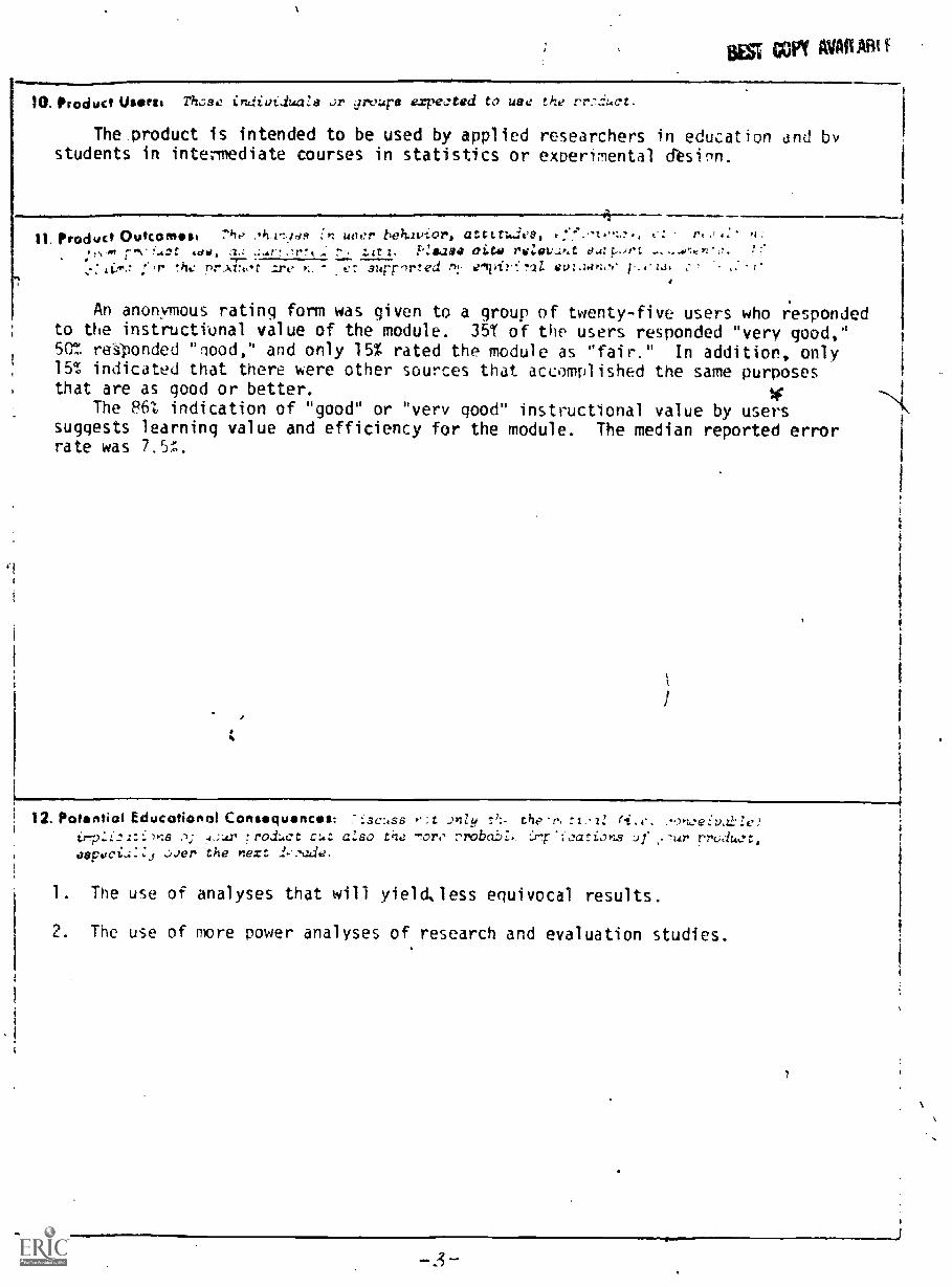
10. Product Were* Those indioiduals Jr groups expected to use the rr.-7th..c.t.

The.product is intended to be used by applied researchers in education and bystudents in intermediate courses in statistics or experimental desi7n.

11. Product Outcornst 7ht., .1.1`111$19 WW1' behilkOri at t ttlide ": 7 , : r. n

.01 ad t ..!1" t z. Nsasa cite re:fift.:,;$,,t dar r,ix$ 4 ,r !he pr..1.07cC r r. Surrwred irstpi!.:.?24 /...'1,3,

An anonymous rating form was given to a group of twenty-five users who respondedto the instructional value of the module. 35T of the users responded "very good,"50% responded "load," and only 15% rated the module as "fair." In addition, only15% indicated that there were other sources that accomplished the same purposesthat are as good or better.

The 86Z indication of "good" or "very good" instructional value by userssuggests learning value and efficiency for the module. The median reported errorrate was

12. Potential Educational Consequences: .:sc :.ss the-r,roduct cut also the -7oro 7robaC)Z, .4-catio s f ..7ar rrc;dz t,

.:;Jer the next _'.-.fie.

1. The use of analyses that will yield,less equivocal results.

2. The use of more power analyses of research and evaluation studies.

3

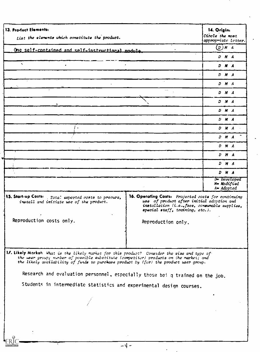
13. Pre 4uct Elententit

List the elements which constitute the product.14. Oigin:

C ii.cle the wetappropqate letter..

. .1 , i'll tit I r ii A 1D M A

D N A..may.. . D Al A-........---....

. .

D N A

D M A

,.. D N A

D N A

ll N Af< D N A

D o r a

D N A

D M A

D M A

D N Aeve opt?,

Nag ModifiedAar Adopted- =a1MIMInwwww

13. Start-up Costs: . Tyrar atpected costa to procum,in,staLl and initiate use of the product.

Reproduction costs only.

16. Operating Costs: Projected costs for continuinguse of product after initial adoption andinstallation (i.e_, fees, consumable supplies,special staff, training, etc.).

Reproduction only.

1/. Likely Markett that is the likely market for this product? Conalder the size and type of-the user group; n:.),:ber of possible substitute (coivetitor) products on the market; andthe likely availability of funds to purchase product by (for) the product user group.

Research and evaluation personnel , especially those bei q trained on the job.

Students in intermediate statlstics and experimental design courses.

.

Instructional Module on the Analysis of Covariancea

This paper discusses the nature and principal uses of the analysis of

covariance (ANCOVA). As Fisher (1934) has expressed it, the analysis of.covariance

"combine the advantages and reconciles the requirements of the two very widely

applicable procedures known as regression and analysis of variance."

In experimental and quasi-experimental studies covariance can perform

two distinct functions. One is to remove bias, that is, statistically equate

groups on some confowiding variables. In quasi-experimental studies coping with

bias is typically its primary function. However, even if there are no real

differences between the two groups on the covariable, hence no danger of bias,

covariance may still be valuable for increasing the power of the analysis.

The Use of ANCOVA

To remove the effects of confounding variables in quasi-experimental studies.

In research endeavors in which randomized experiments are not feasible,

two or more groups differing in some characteristic such as age, can be studied

to discover whether there is a significant difference omong groups on the dependent

aThe ANCOVA overview is adapted from portions of W. S. Cochran's article inBiometrics (13:261-278), 1957.

2

f

variable when groups are statistically equated on the charapritic on whi'ci,

they differ (such as age, LQ, or prete:A score). i'vu:17,1r:, whore tsu,

are not practicable or possible are studies constrastino (.ros,-cultural ;tudies,

social class studies, urban vs..-rural, school districts, etc. In quasi-.

experimental-studies it is Widely realized that an observed association, even

If statisti,(,:al lx significant, may be due wholly Or partly to other disturbing

variables Xl, X2 ... in which the groUps differ, i.e.,.X1 and X2 are threats

to the internal validity of the study 4here feasiblie, a common device is to

matcn the )roups fdr the disturbing variables thought to be most important. This

catching often results in serious problem (cf. Hopkins, 1969). In the same

way., tne analysis of the X-variables can be treated as covari tes and ANCOVA

be employed to extricate the influence of X-variables, st partially.

Ica.,:oiri.son of the heights of children from two different types of

(1953) found that the two groups differed slightly, /though

not -:,ficantly, in mean age. A covariance adjustment for age resulted in a

Lor, cco.parison of the heights. Anotner study statistically equated

d' i n;)-rot,11-c. students do IQ when examining achievement consequences

of school districts have been compared pupil achievement after

cuvaryinq on numerous socio-economic variables.

UnfortOnately, quasi-experimental studies are subject to difficulties

of interpretation from which true experiments are free. Although covariance

rids Seen skillfully applied, we can never be sure that bias, may not be present

from some disturbing variable that was overlooked. Indeed, unless the covariate

is pe-fectly reliable, ANCOVA doeS not remove all of the bias due to X itself.

In true experiments, the effects of all variablesc

measured and unmeasured, real

and illusory, are distributed among the groups,* the randomization in a way

that is taken into account in the standard tests of significance..

.'

There is no such safegtard in the absence of randomization.

. Secondly, when the X-variables show real differences among groups -- the

case in which adjustment is needed most -- covariance adjustments involve

a greater-or-less degree of extrapolation. To illustrate by an extreme case,

suppose that we were adjusting for differences in parents' income in a comparison

of Orivate and public school children, and that the private school incomes ranged

from $10,000-$12,000, while, the. public school incomes .ranged from $4,000-$6,000.

The covariance would adjust results so that they allegedly applied to la mean

income of $8,000 in each group, although neither group has any observations

in which incomes are at or even near this level.

Two consequences of this extrapolation should be noted. Unless the statistical

assumption of linear regression holds in the region in which observations are

lacking, covariance will not remove the bias, and in practice may remove

only a sTall part of it. Secondly, even ff.the regression is valid in the

"no mdn's land," the standard errors of the adjusted means become large, because

the standard error formula in a covariance analysis takes account of the fact that

extralation is being employed (although it does not allow for errors in the

for- c' tne regression equation). Consequently, the adjusted differences May

become insignificant statistically merely because the adjusted comparisons are

of low precision.

When groups differwidely on some'confounding'variable X, these difficulties :

imply that the 'interpretation of al-adjusted analysis is speculative rather than

definitive. While there is no sure way out of the difficulty, two precautions

. are wortn observing.

1. Consider what internal evidence exists to indicate whether the regression

is valid in the .region of extrapolation. Sometimes the fittihg of a more complex

regression formula serves as a partial check.

it.

2. Examine the standard.erors of the adjusted group means, particularly

Oen differences become non-significant after adjustment. Confidence limits for

. the difference in adjusted means will reveal how precise or imprecise the

adjusted comparison is.

410

8The Use of ANCOVA

To increase power.

The use of ANCOVA to increase power in true experiments is frequently

overlooked. The covariate X is a measurement, taken or available,oweach experimental

unit before the treatments are applied, which correlates with the dependent

variable Y. This first illustration of the covariance method in the literature

wAs of this type (Fisher, 1932). Th variate X was the yield of tea per plot

in a period preceding the start of e experiment, while Y was the tea yield

\)at the end of a period of application of treatments. Adjustment of the responses

Y for their regression on X removes'the effects of variations in initial yields

from the experimental errors, insofar as these effects are measured by the

linear regression. 'II. this example these effects might be due to either

inherent differences in 'the tea bushes or to soil fertility differences that

were-permanent enough to persist during the course of the experiment.

With a linear regression equation, the gain in predision from the covariance'

adjustment depends primarily on the size of the correlation coefficient p between

Y and X on experimental units. that receive the same treatment. If 0-12, is the error

variance when no covariance is employed, ANCOVA reduces this error variance to

a value which is about

c4(1 p2)(1 71-127)

-4111

5

,

where fe

is the degrees of freedom associated with the error term. The factor

involving fe ts needed to 'take account of errors in the estimated regressiou

coefficient. If, or the correlation of covariate and the dependent variable, is

less than 0.3 in absolute value,. the reduction in variance is inconequential

.(les, than 91, but as p increases sizeable increases in .precion are obtained.

In-Fisher's example ;'.was 0.928, reflecting a high degree of stability in relative

yield of a plot from one period to another. The adjustment reduced the error

variance roughly to a fraction (ii- (.0.928)2), or about one-sixth, of its original

value. Some of the most spectaculargains in precision from covariance have

occurred ih situations like this, in whiCh the covariate represents an initfal

calibration of the responsiveness of the experimental units.. In educational

studies.it is usually relatively easy to find pretreatment measures that

_correlate .6 or higher with posttestmeasuivs`thereby reducinlg the error term

0

by 36 or more -- approximately the same gain in power that Would result from

doubling the sample size.

In tne use of ANCOVA to increase power, its function.is the same a, that of

stratification and blocking. It removes theeffects of an environmental source

of variation that wOuld otherwise inflate the experimental error and hence the

error mean square. When the relation between Y and X is linear, covariance and

blocking can be about equally effective. If, instead of using covariance, we

can group the subjects into block such that the X values are equal within a

block the error variance is reduced to a2(1 p2).

In a covariance analysis, the covariate X may be measured on a completely

different scale from that of the dependent variable Y. Bartlett (1937) used a

visual estimate of the degree of saltiness of the soil to adjuit cotton yields..

,Federer and ScholOttefeldt (1954) used the serial:order.(1, 2, ...7) of the plot

within a replication as a basis for a quadratic regression adjustment of tobacco

41

4

data, thereby removing the'effects of an unexpected gradient in fvtility within

the replications. Similarly, the reading performances of children under different

methods of instruction may be adjusted for variations in their initial

Note also that X need not be a direct causal agent. of Y -- it may, for instance,

merely reflect some characteristic of the environment that also influences Y.

When ANCOVA is used in this way, it is important to verify that the treat-/

meats have Wad no'effect on X. This is obviously' true when the X'S were measured

before treatments have been applied, as when plant number shortly before harvest

is used to\adjust crop yields for uneve growth, or as happened in the index

of saltiness used by Ba'tl'ett. When the treatments do affect the ,X- values1 ,

to some extent,'the covariance adjustments take oh)a different meaning. .They-,

no longer merely remove a pnponent of experimental error -- in addition, they

distort the nature of the treatment effect that is being measured. If the higher

perfQrmZince by a.superior reading treatment also improves IQ scores, a covariance

adjustment (which attempts to measure what the means would have been if IQ

means: were equal for all treatments), may remove much of the real t-eatments effect.

ASSUMPTIONS REQUIRED FOR THE ANALYSIS-4F COVARIANCE

Tne assumptions required for valid use of the analysis Of covariance are

the natural extension of those for an analysis of 4riance, namely,

(i) Treatment, block and regression effects must be additive as postulated

by the model,

(ii)theresiduals,..(differences between observed and predicted scores

.withinleach treatment group) must be normally and independently distributed

with zero means and the same "sari ante.ate,

7

Much of the related wdrk regarding the effects of.violating statistical:./ .

assumWons on the analySIs of variance eta tends logically to ANCQVA --for

instance the practical unimportance of the additivity assumption (see Glass,,.

` Peckh4m, and Sanders, 1972, p. 241). Table I summarizes an abundance of

research literatUre on pile empirical consequence of violating assumptions in

ANOVA.

Certain qualifications of the conclusions in Table 1 are regarded in the

extension to ANCOVA. For example, non-normality in the dependent variable

inconsequential in ANCOVA only if the covariate.is normally distributed (which

in itself is not, necessarily assumed in ANCOVA).

ANCOVA makes three assumptions that involve the regression term in covariance;

(I) the regression lines for each group ire assumed to be parallel, i.e.,

61 = s2 LL,J. If this is violated, the covariance adjustment may still

improve the precision, (i) the meanings of the adjusted treatment effects

became- cloudy, and (ii) if covariance is applied in a routine way, the

investigator fails to discover the differential nature of the treatment

effects -- a point that might be important fir practical applications.

Peckham (see Glass, Peckham, and Sander 1972) found that violation of0

.the parallel'regression slopes to be tnc sequential in a.one-factor fixed-

effects ANCOVA for a wide variety of conditions. The effects in more complex

factorial design with mixed and random models appears not to have been studied.

(2) The covariance procedure assumes that the correct form of regression

equation has been fitted. PerhapsIthe most common error to be,aaticipated is

that linear regressions will be used',when the true'regrssion is' curvilinear.

In a randomized experiment, the randomization insures that the usual interpre-

1

tations of standard errors and tests of significande are not seriously vittated,

although fitting the correct form of regression would presumably give a larger

'Are of Velem*

ems iodepewdenceof mom

*neormality:libenwess

!trim*

IderogessemetVendome

Table 1

Summary of Consequences of Viokstion of Assumptions of the Fixed-effects ANOVA

Awe/ Unequal m

Effort (m(mil PA

a r a us r o w e r W e e r ore a _Effect ort roarer

Noninekpendence of errors 'Moistly affects both the level of significance and power of.** Fiast regardless whether mil amines, or tompu.d.

Stwirod populations have wiry little effect on either the level of significance ite the power of the Ithedffects model r-telit.distorties; of nonskidsignifiretwo levels of pow" values ate rarely greater them a few hundredths. (Ifiswever, skewed populations can seriously af Iasi the lend of significameeand power of dirertioasi-or mooe-tailar- few )

Actual- a islivis than minima awhen populations are leptaksidlc(i e , 0:>3) Actual a exceedsnominal a for piiitykurtic porde-Same (pert. are With'.

Very diets effect cm a, which isarklom distorted by more than alfew hundredth& Actual * seemsalways in be .lightly lemmaaver the Pontine' o.

Actual power le ken than *optimalpower vdsom,pumiletioste are phi.tykurtic. Actual pope, emceed'nominal pewee when populationssee lvidoktutic. Bifida can hesubstantial for mall a.

(No theoretical power stellar*sista when variances me helm-gepeom.)

Actual a is WM then muninal awhen pripuletions are legtokurtic(i.e.. Oi>3). Actual a exceedsrtnntlital a for platykurtic purge.num. (Effects are sight.)

a may be seriously affected.Actual a exceeds nominal a whensmile" samples are drama frommore veriable populations: actuala ja lees than nominal it whenmallet samples are draws fromism lie Sable populations.

Actual pewee-s Ives than 1101114001puss" whem.populationa are OPtykurtic. Actual powde.itsceed.nominal power when pdirulatioars"-::are leptolturtic. Effect' can be.,substaistal for emelt a's.

(No theoretical pewee settleexists when wham an Wino-seseaae.r

%Pained monotasalityad bet engetwoosmemo

a From Glass, Peckham, and

Nomsormislity and hethrogeaeous melamine wpm to comblair edditively ("modimerectively") to affect either level of eigairwance or octeree. (roetrample. the &mewing effect on a of leptolturtmle could be expected to be counteracted by the elevating effect om 0 at having drawn unlike samplefrom the mote eerie* leptolturtk populitIons.)

n ers (1972).

increase in precision. The.danger of misleading results is greater when the c,

are real differences from `treatment to tr,.:atment on the c:oVa_ciate. Fortunately,

most cognitive and psychomotor variables are linearly related, and unless

measurement procedures are faulty (e.g., a test that laCks''Ceiling), the liinear

regreion model works well in most app cations (see Li, 1964,.for tre4ment ofe

curvilinear ANCOciA). Frequently, curvilinear relationships can.be made.linear

by mathematical transformations of e4he'r the dependent variable Y, or the

.covariate X, or both.

(3) An assumption of ANCOVA that is not widely recognized is that the

covariate is fixed and measured without error. Lord (1960) has shown how.large

errors in the covariate can produce misleading results. The effects of the

less-than-perfectly-reliable covariate are usually predictable 'so the nature of

the bias in the adjustment can be considered in any interpretation. It should

be emphasized, however, that, to the extent the covariate is unreliable, the

statistically equating of the groups is incomplete.

9

10

Illustrative ANCOVA Problem

Suppose therAire three intact gr6ups (A, B, C), each was -given a treatment.They were pretested (X) before the treatment and posttested following thetreatment. The data are depicted graphically on the X and Y axes in Figure 14.

Summary Data

LY

EX2

z:Y2

xY

Means

Treatment

A B

2

45

86

"X Y X

5 14 7 208 16 8 18.7 15 10 239 19 13 25

11 11, 12 24

Y

20

22

26

2824

Totals

25 I 75. 110

40 i 50 120

145 1159 2454

340 526 2920

215 755 2670

5 8! 15 10 1 22 24

ZO

15

20

34

5

26

Total Data (S)

SXX

= 818

Sxy

= 700

SYY

= 846

34

30

40

(X) (Y.)

210

210

3758

3786

3640

X.=14 Y.=14

Within Treatments (E)88 = E

XX

50 = Exy

86 = EYY

Between Treatments (T)

Txx

= 730/

Txy

= 650

TYY

760 \!

Let's ignore the pretest differences for the moment'and perform simple ANOVAon the Posttest (Y).

SV . SS df MS

Treatments 760 2 380 53.1 .01error 86 12 7.16

Total 846 14

I

Figure 1A. Relationship between covariates and dependent variablesk:for samplesproblem.

12

ObViously, this highly significant difference in posttest means is not verymeaningful in light of the pretest differences. To confirm our suspicion thatthere were non - random systematic differences between groups Rrior to the treat-ments, we run an ANOVA.on pretest scores (X) and find that there were highlysignificant d fferences among groups prior to the treatments.

\\\pow, the crucial question is: when we statistically equate groups on the pretest,ould there continue to be significant differences in posttest means. ANCOVAallows 0 to adjust the total sum of squares on the posttest (S ) to (1)remove pI'edictable portions due to differences in pretest means (the "correcting"for bias fIction of ANCOVA) and (2) take advantage of predictability of posttestscore from retest score to reduce our error term (tile power function ofANCOVA). 0

SV SS df

Treatments 730 2

error 88 12

Total 818 14

MS

1165 49.8 <.017.33

. '

To adjust total sum of squaregi)SYY.

2(Sy

)x

S' S 846YY YY -)z)c

To adjust sum of squares error, E :

YY

247

(E)2E' E 86 (5°' 57.6YY YY Exx

88

To adjust treatment sum of squares, T :

YY

TYY = S'Y

ElY

= 247 - 57.6 = 189.4YY

Tne summary ANCOVA table is shown below:

SV SS' df MS'

Trealtments 189.4 2 94.7 18.07 <.01errors 57.6 11 5.24

Total 247.0 13

(Note that one df is lost from error for each covariate)

13

We therefore conclude.then that there are differences among the adjusted posttestmeans that are not explicable solely in terms of initial pretest differences.

For purposes of interpretatiOn, we need to adjust the postttest means:

Xa = Yj - b - Towiis the adjusted mean of\ the jth group. Except for b

w'all the information

-needed to adjust the means\is given in the summary data.. The regression coefficient,bw, is the pooled estimate ,of sw, the "average" slope within the treatment groups.

Eybw °V = .57

xxdr \

Tne adjusted means of the treatment groups are then:

YA . 8 - .57(5-14) = 8 - (-5.1) = 13.1.

= 10 - .57(15-14) = 10 - (.57) = 9.43

= 24 - .450(22-14) = 24 ( 4.6) = 19.4

Figure lB shows a regression line with slope bw fitted to each of the three

gro4ps. The extension of this line to the point at'which it intersects with thegraHd mean of the covariate, X., is the adjusted mean for the group.

Now is the assumption 5A s = sc, which legitimizes pooling, tenable?

To test Ho: eA . sB . sC'

we need to compare the sum'of squares from the pooled

regression line fitted for each group (E;y) with the sum of squares allowing

each group to "find" its own best fitting individual regression line. Figure1C gives the best fitting (least squares) regression line defined separatelyfor each group together with the pooled regression line with slope bw. Of

course the regression line bA will fit group A be91 er than any other regression

line including the one with slope bw. Likewise A and bc give least error

for groups B and.C. The real statistical concern i whether or not bA, las, and be

differ significantly, that is, is Ho: aA = BB = st t nable? If 1-1; is tenable then

the use of the pooled regression.coefficient bw is legitimized.

. We already have obtained the error sum of squares using the pooled regressioncoefficient b

NI Y, i.e., Et

Y= 57.6. The error sum of squares for group A

using bA is: \

(E,.....

AA)2

-. E -20 81 8.EL

-"A A Exx2u

(1512

A

14

. .

Figure IB. An illustration of the process of adjusting means forpretreatment differences.

15sw, 10041

f

....7y2 from b"..,2 frorr

,

>,.120,.= .57

6 8 12 14

B-15

p

'8 2C 2- 24 a 28 30

Figure 1C. The relationship between regression lines defined byseparate groups with the regression line employingpooled data.

16

Similarly for groups B and C using bB and bc respectively:

E' = 25.3, E' = 13.5YYB

Eby

For convenience define SI = EE' = error sum of squares when each group definesYYj

its own best fitting regression line.

SI = 8.8 +'25.3 + 13e5 = 47.6

The reduction in sums of squares when best fitting individual regression linesare %used (i.e., bA, bB, and bc) in lieu of regression lines with the regression

coefficient based on the pooled information(big), is defined as S2:

S2 = E;y - S1 = 57.6 - 47.6 = 10.0

Obviously, if bA = b8 = bc02 would be zero.

To test the significance of the non-parallelism in the individual regressionlines:

F

S /(J10.0 2

477u376.= .945 the F-ratio is below 1.0 -- obviously

1

not significant.

In setting up confidence intervals about adjusted means and/or making multiplecomparisons, MS; is not used, but MSS which is larger than MS; to the extent

that the groups differed on the covariate, i.e., if T = 0, MS"e

= MS'..xy

pgsy n ms"

Txx/(j_i)

e 6 1 +

17

ANOVA Computational Problem Set

'Fifteen subjects were administered a non-reactive pretest (X) and were randomlyassigned to one of three treatments. The pretest and.posttpst data appear below.(Winer notation; problem taken from Edwards).

Treatmept Group

1 2 3

If X Y- X Y

1 5 2 1 1 106 12 3 '2 4 133. 9 6 7 5 164 8 4 3 3 125 11 7 8 6 17

Summary Data

.-E ( )

1: ( )2

EUMeans

XYIX19 45

87 435

191

3.8 9.0

YX1

1

1 22 21 1

i

1114 127 1

i118 1

14.4 4.2 '3.8I

I

1 J

Totals(X) (Y)

19 68 60 134

87 958 288 1520

270 579

13.6 4.0 8.93

CL) (V. )I_ -

Within Groups Data (E)

2 Exxj

xxyj = Ev

4i2 - E

Y Yj

14.8

20..0

.30.0

117.2

1

I 25.61

38.8

1 14.8 46.8 Exx

1

1 21.6 '67.2 = E,,1 1

33.2 ; 102.0 = E1

YY

Total Data (S) Between Treatments i )

SXX

= 48.0

Sxy = 53.0

SYY

= 322.9

TXX

= 1.2

Txy = -14.2

TYY

= 220.9

18

1. Plot Y values against X values for each group. (Use different colors ormarks for each group for visual seraration.

Following each exercise is a dotted line, below which provides the answers'to the questions posed in the exercise. Attempt each question beforeconsulting the anstter.

2. Perform an analysis of variance of the posttest scores (Y) so that we maylater compare the results with those from ANCOVA.

SV

Treatments

error'

SS df F

102.0

.220.9/2 = 110.45; 102.0/12 = 8.5

3. Now perform ANCOVA covarying on X

2 12.99

8.5

(.99F2,12 = 6.93)

Adjusted total(5, )2

SUM of squares,S' = Sr,, ( ) - 264.4YY xx

322.9 1r2

67.24. E' = )

(46.8 )232 102

-5.5 = Adjusted error sums of squaresYY

E. (E )2/Eyy xy XX

5. T' = ( ) - ( ) = 258.9 (Not Tyy xy

)2/Txx

; this is affected byYYerror in estimating B froni b 's.)

S - E'YY YY

6. Therefore:

SV SS df MS F.

Treatments (TL,) 129.45 258.4

YError (E'

Y) " .50

.99F2,117.21

258.9/2; 5.5/11

19

7. degree(s) of freedom is (are)' lost for each covariate employedone in thisopxample), which accounts for the Blight (increase

or decrease) in the critical F-ratios.

ncrease4 .0 O

8. Why didn't T;fy and Tyy differ greatly as they did in the earlier illustrative -1

problem?

because the group means .on the covariate differed,mi wily, hence thee.'unadjusted means did not differ greatly from the adj steel means..

9a. WillTy,

aslarger than T- as a general rule in true expeilments, i.e.,

when random assignment of.subjecfs to treatments has "been employed?

no, no consistent trend

9b. When will T' ?YY YY

when rxy

0 (within cells), or when Y1 =.72 = ...=xj

10. .When. will EY' = E 7Y YY. C

odly when txy (within cells) = 0, hence bw = 0.0

11. The relative .adtiantage of ANCOVA over ANOVA can be seen best by comparing'which one of these?

a. E'YY

with

b. T'YY

with

c. S' withYY

d. computed

a.

YY

syy

F-values

12: The again in the power of ANCOVA over ANOVA is shown by the ratio of MS; to

or, in this example, .50/8.5.

MSe

13. The gain in precision is a direct function of the correlation between theand the ,dependent variable (within cells, it is not rxy for all

observations combined).

covariate

20

14. MSe = MSe(1 - r2), therefore i.n this problem: (= means "approximately equal to")

r2 a 1 1 = 1

e e

- .059 =

E 2Xy

15. More precisely, ri = E for each group, or pooling our within groups4 XX. yy.

J J

, information:.

E 2

r2w E

.946xx yy

(This ,uncommonly hi4h r is the reason MS' and-MSe

differ sodrastically.)

.4..

16. In orde to adjust the Tj values to values we must find the pooledwithin -c 11 regression coefficient, bw.

.= ir. - b (3(J : 3( )wE

b = = 1.44xx

67.2/46.8

11

17. This value indicates that for every unit deviates from the grand meanof the covariate, it will.be expected to deviate units from the

grand mean of the dependent variable, ir

1.44 .-

18.1

=1-

bw 1

7.) ( ) - 1.44 ( ) = 9.0 + .29 = 9.29-=

9.0 - 1.44 (3.8 - 4.0)

19. Since group A was below the grand mean T(% TA would be (smaller

or larger) than TA. ,

larger.

20.2

( ).

- bw

( )(X - X.) = 4.2 = 1.44(4.4 -41.0) = 3;62

21

I

21.3

13.6 - 1.44(3.8 - 4.0) = 13.6 + .29 = 13.89. The grand mean of the

usted means, Trt = (4en n's are equal), is

J( ( ) ( ) 26.80 8.93.

3 3

(9.29) + (1.62) + (13.89)3

22. Does = V:? Will this always be the Lase?

Yes. Yes.

p

Now let's to to the question of evaluating our assumptions. (Ideally, oneshotild do thts prior to performing the analysis.)

23. An assumption in ANCOVA is that the within -group regression lines arelarallel. In more symbolic form:bl, b2 ... 1).

jdiffer only randomly feom

the parameter, ; or equivalently; $1 = $2 = = Bj

h.

24.-Itiordertotesti.10:81'=0c,;-......-0.0ne compares the pooled variation

within each group about it own best - fitting regression line, with thepooled variation within groups about a regression line with the common"average" slope,.b . We-have already computed the latter, which carried the

symbol: = 5.5.A

G.

E'

YY

i

25. .Now the E'YYI.,.

alues (allq#i g each group to defihe its own least-squarps,

, Iregression line) are given by: %

(E )2xy n 2

EYY.' = EY

E.--1--; e.g., E' = 30 iii 2.97.3 YJ XX. "1

E' = i .70; E' = 33.2(14.821.6)2

1.68312 yy3

38.8 -(25.6)217.2

22-.1«

-- _-

26. Then the variation within each group about its own best-fitting regression;summed for all groups, S1, is + + = 5.35.

(Note that S1 does not refer to group 1 but is total 'sum of squares-when

each group is allowed to define its best fitting regression line.)

2.97 + .70 + 1.68

1.)

27. Obviously, S1 (can or cannot) exceed E;v

cannot

28. When would S1 y

= Eby ?'

when all cells had precisely the same regression coefficient, i.e., bi=b2=b3=bw

29. S1 Y

and E'Y

should differ only randomly if Ho

: is true.

51 62 N= 6j

30. The difference in unpredictable variance, allowing each group to use itsown regression.coefficient in predicting'Y from X, from that in which alluse the pooled value is then: S2 = ( ) ( ) = 5.5 - 5.35 = .15

E - Syy 1

31. By dividing S2 and S1 by their respective degyees of freedom, (J - 1) and

J(n -2), we have two unbiased estimates of population variance which willfollow the central F-distribution when Ho: 81 = 82 = = 8j is true.

.52/(J - 1)

F

1

t(Q- = .126'

(.15)1(2)

(5.35)/(9)

32. Is it necessary to reference the F-table? Why?

No, if F < 1, Ho is never rejected in the typical (one-sided) F-test.

The test of linearity is considerably more involved, the basic rationale being,by allowing a quadratic, or cubic, etc. expression into the regression equation,to give the best-fitting curvilinear regression line, would the 42 be significantJess for the curved regression line thdh for a single straight line ? The researcher;usually knows from previous study,th variables which are more likely to berelated in a non-linear fashion, i.e., personal, social, affective variable.Curvilinearity may be removed by certain transformations or it may be built inan.ANCOVA del (cf. Li, J. C. R., Statistical Inference, Vol. II, 1964). Theprocedures 'n a factoriAl design ari5eiiiii7TEFFeTTbeing analagous to thegroup in th present_ example.

Comparing ` ANCOVA With Other Analysis Strategies.

It is interesting to compare the ANCOVA results with the probable results had,a randomized blocks design been used, blocking on pretest scores.

SV

TreatmentsBlocksError

SS df MS F

220.9 2 110.45 235.0298.3 4 24.563.7 8 .47

322.9

33. The MS' from ANCOVA is slightly (larger, smaller) than the error MS

from the analysis from the randomized blocks design.

larger

34. However, the error term in the latter analysis is )hk.sedr on(8 vs.......) degrees of freedom which requires a (larger,in order to rejec. H

0.

.

In this case for ANCOVA7-7-795 2,11 3

for the randomized blocks design, .95F2,8 = 4.46.

fewer; 8 vs. 11; larger

(fewer, more)smaller) F-value

.89, and

35. The randomized blocks analysis is more "robust" in Chat it is free fromassumptions of parallel regression lines and implicit in ANCOVA.

linear regression

36. Edwards (1960) performed an ANOVA of the same data using gain scores (posttest-pretest) for each subject

SV - SS df

TreatmentsError

250.514.4

264.9

It is evident in comparing error(more, less) efficient t an the ANCOVA and randomized blocks

design.

MS

2 125.31.2012

F

104.4

values, that the latter analysis is much

less

24

Post Organizer

ANCOVA can be a useful statistical tool both for true and quasi-experiments.

Its two potential advantages over ANOVA are (1) statistical compensation for

pretreatment differences or'bias, i.e., removing various "selection!' threats

to the internal validity of the study, and (2) increasing the power of the analysls.

With respect to the bias removing function it is important to be aware that

pretreatment differences may exist on certain unmeasured variables, hence the

adjutAments are never complete and impeccable. In addition, the statistical

comnensation will be incomplete to the.extent that the covariate is ynreliable.

ANCOVA cannot bring results from a quasi-experiment to the same-tevil of

credibility allowed by a true experiment.

Regarding the increase in power function, ANCOVA can make a substantial

contribution to true experiments. If the covariate (or combi.:ation or covariates)

correlate about .7 with the dependent variable within groups, the .gain in power

is approximately the same that would accompany a four-fold increase in N.

There are other design and analysis strategies for capturing this.g in

power, the most common of which is blocking or strati\fying on the X-var ble.

These alternatives are generally preferable if the experimenter has complete

control over the conditions of the study since the unique ANCOVA assumptions

are of no concern and stratifying allows one to detect interaction effects

between the treatments and the X-variable.

The basic ANCOVA rationale extends logically to multiple covariates where

the covariates are the predictors in a multiple regression context.

V

AR

I

A

E.

Covariate

Mastery Test on ANCOVA

II III

X x X

Covariate Covariate

1. By examining the situations depicted above, how does the adjustedMS'

treatmentsfrom ANCOVA, compare to the MS

treat ntshad the covariates

been ignored and an ANOVA performed?

MS'treatments

would differ little in situations and , and

increase in situation

In which situation will the adjusted error mean square, MS;, differ

little from the unadjusted error mean square, MSe?

3. The gain in power from ANCOVA over ANOVA appears greatest in situation

4. Do the data suggest any serious violation of ANCOVA assumptions?

5. Which situations appear to represent quasi-experiments?

5. In which situation are the results from ANCOVA would be almost identicalto those from ANOVA?

7. In figure I, the adjusted mean of the E group would be nearest of pointa, b, or c?

An additional covariate appears to be needed least in situation I, II, or III?

9. Otner things being equal, in which situation has the smallest adjustederror mean square, MS;?

10. bw

in group II is about

ANSWERS:I. TT and III, I 6. II

2. II 7. C

3. III 8. III4. No 9. III

-5. I and II 10. 0.0

REFERENCES

Cochran, W.G. Analysis of covariance: Its nature and uses. Biometrics, 1957,13, 261-281.

Glass, G.V., Peckham, P.D., & Sanders, J.R. Consequences of failure to meetassumptions underlying the fixed effeds analyses of variance and covariance.Review of Educational Research, 1972, 42, No. 3, 237-284.

Hopkins, K.D. Regression and the matching fallacy in quasi-experimentalresearch. The Journal of Special Education, 1969, 3, No. 4, 329-336.

Li, J.C.R. Statistical Infe ence II. Michigan: Edwards Brothers, Inc., 1964.

Lord, F.M. A paradox in th interpretation of group comparisons. PsychologicalBull., 1967, 68, 304-305.

...,

Winer, B.J. Statistical Pri iples in Experimental Design. New York: McGraw-Hill, 1962; 2nd edition, 1 71.