Embed Size (px)
Citation preview
DOCUMENT RESUME
ED 404 348 TM 026 105
AUTHOR Timm, Neil H.TITLE Full Rank Multivariate Repeated Measurement Designs
and Extended Linear Hypotheses.PUB DATE Aug 96NOTE 28p.; Paper presented at the Annual Meeting of the
American Psychological Association (104th, Toronto,Canada, August 1996).
PUB TYPE Reports Evaluative/Feasibility (142)Speeches /Conference Papers (150)
EDRS PRICE MF01/PCO2 Plus Postage.DESCRIPTORS Equations (Mathematics); *Mathematical Models;
*Multivariate AnalysisIDENTIFIERS *Full Rank Linear Model; *Repeated Measures Design;
Statistical Analysis System
ABSTRACTHypotheses that do not have the standard bilinear
form theta=CBM=0 occur naturally in the analysis of repeatedmeasurement designs. An expanded class of the tests of the formpsi=Tr(G theta)=0, called extended linear hypotheses, provides aricher class of parametric functions. A method to analyze doublemultivariate and mixed multivariate models (MMM) using theStatistical Analysis System (SAS) is demonstrated. The analysis isextended to extended hypotheses, and a new approximate test ofextended linear hypotheses for MMM designs is developed that does notrequire multivariate sphericity, but only a general Kroneckerstructure. Two appendixes provide SAS programs for these methods.(Contains 4 tables and 26 references.) (SLD)
***********************************************************************
Reproductions supplied by EDRS are the best that can be madefrom the original document.
***********************************************************************
1.
Full Rank Multivariate Repeated Measurement Designs
and Extended Linear Hypotheses
U.S. DEPARTMENT OF EDUCATIONOffice of Educational Research and Improvement
EDU TIONAL RESOURCES INFORMATIONCENTER (ERIC)
This document has been reproduced asreceived from the person or organizationoriginating it.
Minor changes have been made toimprove reproduction quality.
Points of view or opinions stated in thisdocument do not necessarily representofficial OERI position or policy.
Neil H. Timm
University of Pittsburgh
Abstract
PERMISSION TO REPRODUCE ANDDISSEMINATE THIS MATERIAL
HAS BEEN GRANTED BY
A)E/Z- N'-----(//4/14/
TO THE EDUCATIONAL RESOURCESINFORMATION CENTER (ERIC)
Hypotheses that do not have the standard bilinear form 0 = CBM = 0 occur naturally in the analysis of
repeated measurement designs. An expanded class of tests of the form yr = Tr(GO) = 0, called extended linear
hypotheses, provide a richer class of parametric functions. In this paper we show how to analyze double multivariate
(DMM) and mixed multivariate models (MMM) using SAS. We extend the analysis to extended hypotheses and
develop a new approximate test of extended linear hypotheses for MMM designs that does not require multivariate
sphericity, only a general Kronecker structure.
Key words: double multivariate model, multivariate mixed model, multivariate sphericity, multi-response, growth
curve model
Paper presented at the 104th meeting of the American Psychological Association at Toronto, Canada, August 1996,Monday, 9:00 am, Kingsway Room.
2BEST COPY AVAILABLE
1. Introduction
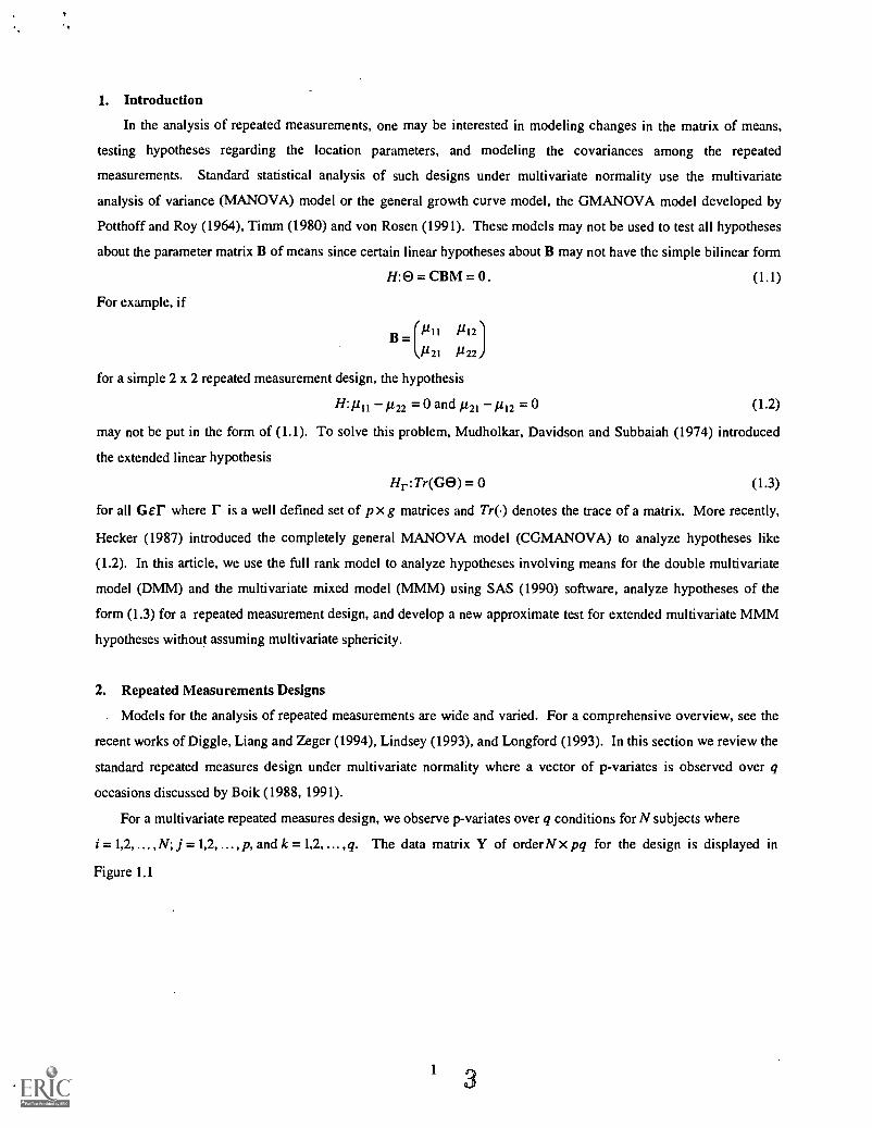
In the analysis of repeated measurements, one may be interested in modeling changes in the matrix of means,
testing hypotheses regarding the location parameters, and modeling the covariances among the repeated
measurements. Standard statistical analysis of such designs under multivariate normality use the multivariate
analysis of variance (MANOVA) model or the general growth curve model, the GMANOVA model developed by
Potthoff and Roy (1964), Timm (1980) and von Rosen (1991). These models may not be used to test all hypotheses
about the parameter matrix B of means since certain linear hypotheses about B may not have the simple bilinear form
H:0 = CBM O. (1.1)
For example, if
B=ril /112)
P21 /122
for a simple 2 x 2 repeated measurement design, the hypothesis
H:gii 1122 = 0 and p21 p12 =0 (1.2)
may not be put in the form of (1.1). To solve this problem, Mudholkar, Davidson and Subbaiah (1974) introduced
the extended linear hypothesis
Hr:Tr(GO) = 0 (1.3)
for all Gel' where r is a well defined set of px g matrices and Tr) denotes the trace of a matrix. More recently,
Hecker (1987) introduced the completely general MANOVA model (CGMANOVA) to analyze hypotheses like
(1.2). In this article, we use the full rank model to analyze hypotheses involving means for the double multivariate
model (DMM) and the multivariate mixed model (MMM) using SAS (1990) software, analyze hypotheses of the
form (1.3) for a repeated measurement design, and develop a new approximate test for extended multivariate MMM
hypotheses without assuming multivariate sphericity.
2. Repeated Measurements Designs
. Models for the analysis of repeated measurements are wide and varied. For a comprehensive overview, see the
recent works of Diggle, Liang and Zeger (1994), Lindsey (1993), and Longford (1993). In this section we review the
standard repeated measures design under multivariate normality where a vector of p-variates is observed over q
occasions discussed by Boik (1988, 1991).
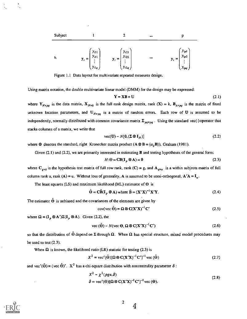
For a multivariate repeated measures design, we observe p-variates over q conditions for N subjects where
i =1,2, ... ,N; j 1,2, ... , p, and k = 1,2, ... , q. The data matrix Y of orderN x pq for the design is displayed in
Figure 1.1
1
3
Subject 1 2 p
SiYi =
(Yil 1
Yil 1
ilq
Yi =
Yi21
Y122
Y i2q j
Figure 1.1 Data layout for multivariate repeated measures design.
Yi =
Yip'
Y ip2
Y.\ I
Using matrix notation, the double multivariate linear model (DMM) for the design may be expressed:
Y = XB + U (2.1)
where YNxpq is the data matrix, XNxk is the full rank design matrix, rank (X) = k, Bkxpq is the matrix of fixed
unknown location parameters, and UNxpq is a matrix of random errors. Each row of U is assumed to be
independently, normally distributed with common covariance matrix E Using the standard vec) operator that
stacks columns of a matrix, we write that
vec(U) - N[0, (E 0 IN)] (2.2)
where 0 denotes the standard, right Kronecker matrix product (A 0 B = fauB}), Graham (1981).
Given (2.1) and (2.2), we are primarily interested in estimating B and testing hypotheses of the general form:
H:0 = CB(Ip A) = 0 (2.3)
where Cgxk is the hypothesis test matrix of full row rank, rank (C) = g, and Aqxu is a within subjects matrix of full
column rank u, rank (A) = u. Without loss of generality, A is assumed to be semi-orthogonal, A'A = I..
The least squares (LS) and maximum likelihood (ML) estimator of 8 is
O = 0 A) where B = (X' X)-IX'Y. (2.4)
The estimator 0 is unbiased and the covariances of the elements are given by
cov(vec = 12 C(X'X)-I C'
where Si = (Ip A')Z(Ip ®A). Given (2.2), the
vec (6) - N(vec 0, 12 0 C(X'X)-I C')
(2.5)
(2.6)
so that the distribution of 0 depend on Z through S2. When 12 has special structure, mixed model procedures may
be used to test (2.3).
When 12 is known, the likelihood ratio (LR) statistic for testing (2.3) is
X2 = vec'(6)[12 0 C(X'X)-I CT' vec (6) (2.7)
and vec'(6) = (vec O)'. X2 has a chi-square distribution with noncentrality parameter 5 :
X2 - x2(pgu,5)
S = vec'(0)[12 0 C(X'X)-ICTI vec (0).
24
(2.8)
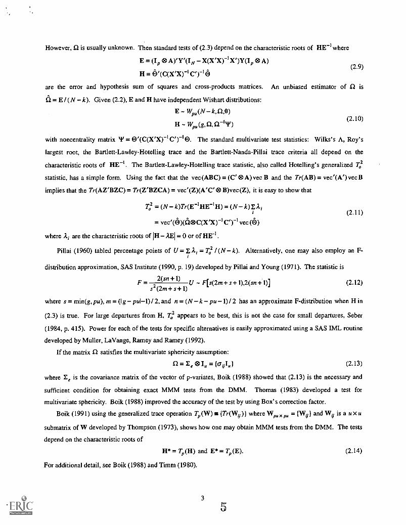
However, SI is usually unknown. Then standard tests of (2.3) depend on the characteristic roots of HE-1where
E = (Ip 0 A)'Y'(IN X(X'X)-I X')Y(Ip 0 A)(2.9)
H = 61(C(X'X)-ICTIO
are the error and hypothesis sum of squares and cross-products matrices. An unbiased estimator of S2 is
= E / (N k). Given (2.2), E and H have independent Wishart distributions:
E W pu(N k, S2,0)(2.10)
H Wp.(g,c1,11-14')
with noncentrality matrix `I' = 0'(C(X'X)-1 C')-10. The standard multivariate test statistics: Wilks's A, Roy's
largest root, the Bartlett-Lawley-Hotelling trace and the Bartlett-Nanda-Pillai trace criteria all depend on the
characteristic roots of HE-1. The Bartlett-Lawley-Hotelling trace statistic, also called Hotelling's generalized Tc ,2
statistic, has a simple form. Using the fact that the vec (ABC) = (C' 0 A) vec B and the Tr(AB) = vec'(A') vec B
implies that the Tr(AZ'BZC) = Tr(Z'BZCA) = vec'(Z)(A'C' B)vec(Z), it is easy to show that
Toe = (N k)Tr(E-'HE -1 H) = (N k)E Ai(2.11)
= vec'(6)(a0C(rX)-1C')-1vec (e)
where Ai are the characteristic roots of 1H AEI = 0 or of HE-1.
Pillai (1960) tabled percentage points of U = I Ai = ,2 / (N k). Alternatively, one may also employ an F-1
distribution approximation, SAS Institute (1990, p. 19) developed by Pillai and Young (1971). The statistic is
2(sn + 1)F = U F[s(2m+ s + 1),2(sn + 1)] (2.12)
s 2 (2m+ s+ 1)
where s = min(g, pu), m = (I g pul-012, and n = (N k pu 1) 12 has an approximate F-distribution when H in
(2.3) is true. For large departures from H, 02 appears to be best, this is not the case for small departures, Seber
(1984, p. 415). Power for each of the tests for specific alternatives is easily approximated using a SAS IML routine
developed by Muller, LaVange, Ramey and Ramey (1992).
If the matrix S2 satisfies the multivariate sphericity assumption:
= me Iu = (0.0u) (2.13)
where I, is the covariance matrix of the vector of p-variates, Boik (1988) showed that (2.13) is the necessary and
sufficient condition for obtaining exact MMM tests from the DMM. Thomas (1983) developed a test for
multivariate sphericity. Boik (1988) improved the accuracy of the test by using Box's correction factor.
Boik (1991) using the generalized trace operation Tp(W) {Tr(Wy )} where Wp.. = j} and Wig is a uxu
submatrix of W developed by Thompson (1973), shows how one may obtain MMM tests from the DMM. The tests
depend on the characteristic roots of
H* = Tp(H) and E* = Tp (E). (2.14)
For additional detail, see Boik (1988) and Timm (1980).
3
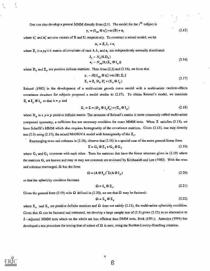
One can also develop a general MMM directly from (2.1). The model for the subject is
yi = (Ipq x;) vec (B)+ ui (2.15)
where x; and u; are row vectors of X and U, respectively. To construct a mixed model, we let
ui = + ei
where Zi is a pqx h matrix of covariates of rank h,2,1 and ei are independently normally distributed:
Nh(0,Dh )
ei Npq[0,(E, 0 Id](2.16)
where Ph and I, are positive definite matrices. Then from (2.2) and (2.16), we have that
yi N[(I )0 vec (B),(2.17)
Ei = Zi Ph Z; (I, ®zq).
Reinsel (1982) in the development of a multivariate growth curve model with a multivariate random-effects
covariance structure for subjects proposed a model similar to (2.17). To obtain Reinsel's model, we associate
Zi =1 lq so that h = p and
= = (Dp 0Iq1;)+ (Le 0 Ig) (2.18)
where Dp is a p x p positive definite matrix. The structure of Reinsel's matrix is more commonly called multivariate
compound symmetry, a sufficient but not necessary condition for exact MMM tests. When E satisfies (2.13), we
have Scheffd's MMM which also requires homogeneity of the covariance matrices. Given (2.13), one may directly
test (2.3) using (2.17), the mixed MANOVA model with homogeneity of the I.
Rearranging rows and columns in (2.18), observe that (2.18) is a special case of the more general linear form
1= GI 0Li +G2 0E2 (2.19)
where G1 and G2 commute with each other. Tests for matrices that have the linear structure given in (2.19) where
the matrices Gi are known and may or may not commute are reviewed by Krishnaiah and Lee (1980). With the rows
and columns rearranged, Q has the form
f2 =(A0Ip)'E(A0Ip) (2.20)
so that the sphericity condition becomes
n=i.eze. (2.21)
Given the general form (2.19) with SI defined in (2.20), we see that Ci may be factored:
c2= Eu Ole (2.22)
where Eu and le are positive definite matrices and SI does not satisfy (2.21), the multivariate sphericity condition.
Given that f2 can be factored and estimated, we develop a large sample test of (2.3) given (2.22) as an alternative to
adjusted MMM tests which on the whole are less efficient than DMM tests, Boik (1991). Ameniya (1994) has
developed a test procedure for testing that of subset of S2 is zero, using the Bartlett-Lawley-Hotelling criterion.
4
6
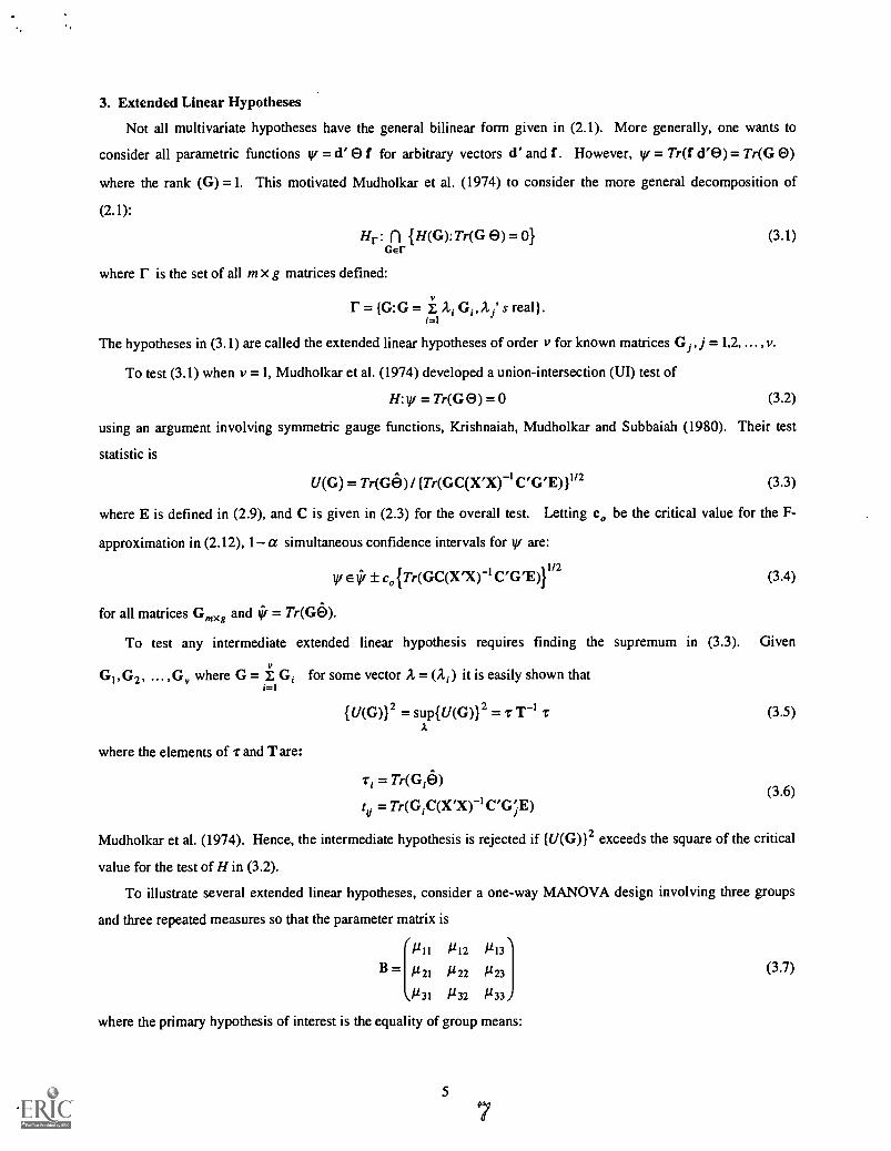
3. Extended Linear Hypotheses
Not all multivariate hypotheses have the general bilinear form given in (2.1). More generally, one wants to
consider all parametric functions yi = d' 0 f for arbitrary vectors d' and f . However, iv = Tr(f d'O) = Tr(G 0)
where the rank (G) =1. This motivated Mudholkar et al. (1974) to consider the more general decomposition of
(2.1):
Hr: (.1 IH(G):Tr(G (3) = 0} (3.1)GEr
where r is the set of all m x g matrices defined:
r = (G: G= E Ai Gi , Ai' s real ) .=i
The hypotheses in (3.1) are called the extended linear hypotheses of order v for known matrices j = 1,2, ... , v.
To test (3.1) when v =1, Mudholkar et al. (1974) developed a union-intersection (UI) test of
H: v/ =Tr(Ge) = o (3.2)
using an argument involving symmetric gauge functions, Krishnaiah, Mudholkar and Subbaiah (1980). Their test
statistic is
U(G) = Tr(Go)/ fTr(GC(XX)-1c,G,E)11/2 (3.3)
where E is defined in (2.9), and C is given in (2.3) for the overall test. Letting c, be the critical value for the F-
approximation in (2.12), 1 a simultaneous confidence intervals for tv are:
yr E ± ITr(GC(X10-11/
(3.4)
for all matrices G,xg and if = Tr(GO).
To test any intermediate extended linear hypothesis requires finding the supremum in (3.3). Given
GI , G2 , , G, where G = E G1 for some vector A = (Ai) it is easily shown thati=i
{U(G) }2 = sup {U(G) }2 = r T-1 r (3.5)
where the elements of r and T are:
A
Ti = Tr(G i6)
tu = Tr(GiC(X'X)-1C'G;E)
Mudholkar et al. (1974). Hence, the intermediate hypothesis is rejected if {U(G) }2 exceeds the square of the critical
value for the test of H in (3.2).
To illustrate several extended linear hypotheses, consider a one-way MANOVA design involving three groups
and three repeated measures so that the parameter matrix is
(3.6)
B = [euil1121
1131
1112
1122
1132
11I3
123
1133
(3.7)
where the primary hypothesis of interest is the equality of group means:
5
7
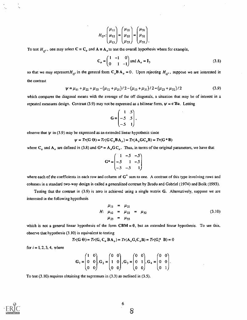
To test HG.
HG':
ill I
1112 =
1121
/222
111231
_1
/131
1232
ii33
one may select C = Co and A E. Ao
( 0 1
to test the overall hypothesis where for example,
Co( 1 1
and A0 = I31
(3.8)
so that we may representHG. in the general form CoB Ao = 0. Upon rejecting HG. , suppose we are interested in
the contrast
V1=1/11 +P22 +/233 -(1212 +Y21)/2-(1213 +/131)/2 -(1123 +1132)12 (3.9)
which compares the diagonal means with the average of the off diagonals, a situation that may be of interest in a
repeated measures design. Contrast (3.9) may not be expressed as a bilinear form, v = c'Sa. Letting
1 .5
G= .5 ,
.5 1
observe that v in (3.9) may be expressed as an extended linear hypothesis since
= Tr(G e) = Tr(G C013 Ao) = Tr(A0GC0B) = Tr(G * B)
where Co and Ao are defined in (3.8) and G* = A0G Co. Thus, in terms of the original parameters, we have that
1 .5 .5G*4-5 1 .5
5 .5 1
where each of the coefficients in each row and column of G* sum to one.
columns in a standard two-way design is called a generalized contrast by B
Testing that the contrast in (3.9) is zero is achieved using a single
interested in the following hypothesis
1111 = /121
H: 1112 = 1122 = 1232
1123 = 1133
which is not a general linear hypothesis of the form CBM = 0, but an
observe that hypothesis (3.10) is equivalent to testing
Tr(G e) = Tr(G ;Co BA0)= Tr(AoGiCo B) =
for i = 1, 2, 3, 4, where
G1
=11
0
0
A contrast of this type involving rows and
radu and Gabriel (1974) and Boik (1993).
matrix G. Alternatively, suppose we are
(3.10)
extended linear hypothesis. To see this,
Tr(G r` B) = 0
0
0
0
, G2 =
0
1
0
0
0
0
, G3 =
0
[00
0
1
0
, G4 =
0
[00
0
0.1
To test (3.10) requires obtaining the supremum in (3.3) as outlined in (3.5).
6
8
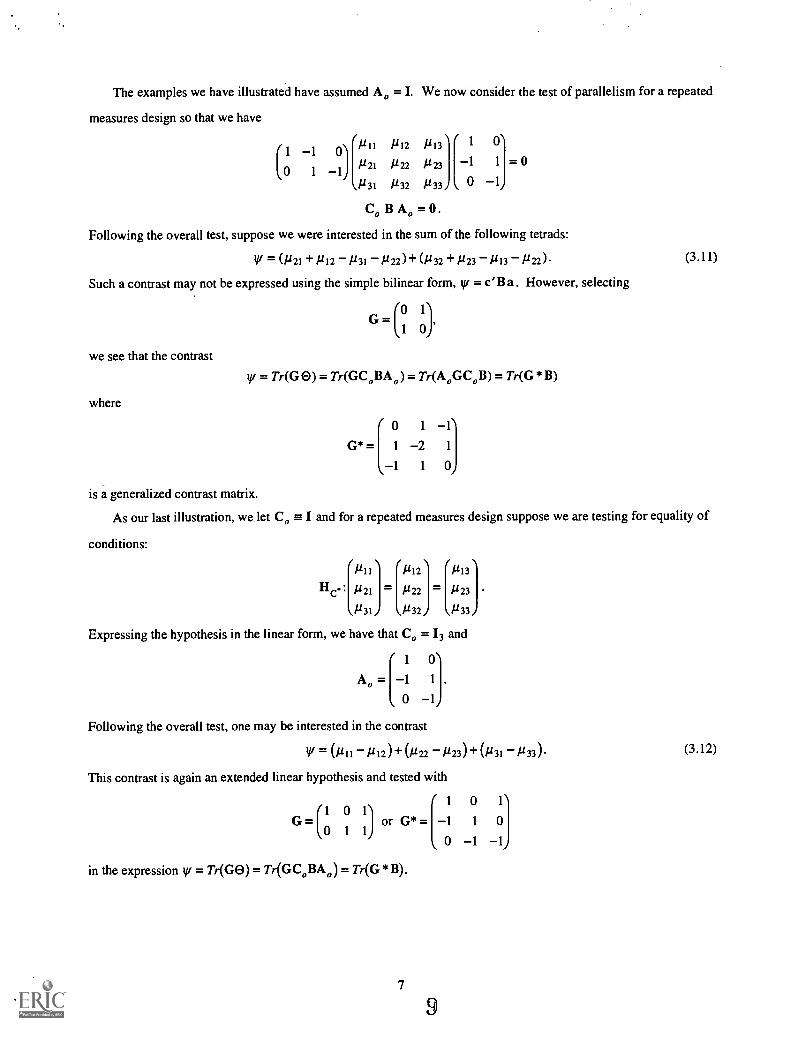
The examples we have illustrated have assumed A0 = I. We now consider the test of parallelism for a repeated
measures design so that we have
( 1
0-1
1 1 #21
#31
#12
1122
#32
#23
1133
1
-10
0
11
1"
Co B A, =0.
Following the overall test, suppose we were interested in the sum of the following tetrads:
= (121 +P12 /131 -1122 )+ (#32 +#23 -#13 -#22)
Such a contrast may not be expressed using the simple bilinear form, tv = c'B a . However, selecting
we see that the contrast
where
G=
= Tr(G 0) = Tr(GCoBA0) = Tr(A0GC0B) = Tr(G * B)
0 1 1G*= 1 2 1
1 1 0
(3.11)
is a generalized contrast matrix.
As our last illustration, we let Co a- I and for a repeated measures design suppose we are testing for equality of
conditions:
He.: [P11]1121
1131
= 1122
1132
= #23
#33
Expressing the hypothesis in the linear form, we have that Co = 13 and
1 0
A0= [-1 11.
0 1Following the overall test, one may be interested in the contrast
= (Yu 1112)+(1122 1123) +(1131 -#33)
This contrast is again an extended linear hypothesis and tested with
1 0 1
1 0 1
G = or G*= 1 1 01 1
0 1 1in the expression yr = Tr(GO) = Tr(GC0BA0) = Tr(G*B).
7
9
(3.12)
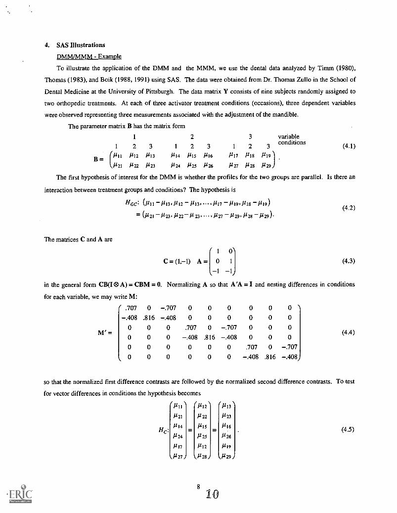
4. SAS Illustrations
DMM/MMM - Example
To illustrate the application of the DMM and the MMM, we use the dental data analyzed by Timm (1980),
Thomas (1983), and Boik (1988, 1991) using SAS. The data were obtained from Dr. Thomas Zullo in the School of
Dental Medicine at the University of Pittsburgh. The data matrix Y consists of nine subjects randomly assigned to
two orthopedic treatments. At each of three activator treatment conditions (occasions), three dependent variables
were observed representing three measurements associated with the adjustment of the mandible.
The parameter matrix B has the matrix form
1 2 3 variable
1 2 3 1 2 3 1 2 3conditions (4.1)
(1117 PI8 1119PII P12 P13 /114 PI5 P16
/121 P22 P23 P24 P25 P26 P27 P28 P29
The first hypothesis of interest for the DMM is whether the profiles for the two groups are parallel. Is there an
interaction between treatment groups and conditions? The hypothesis is
HGC: 0111- g139P12 P13, , PI7 -P199 P18 -P19)(4.2)
B=
The matrices C and A are
= (P21 -P23, P22 -P23, 9 P27 -µ29,µ28 -P29).
1
C=(1,-1) A= 0 1
1 1(4.3)
in the general form CB(I 0 A) = CBM = 0. Normalizing A so that A'A = I and nesting differences in conditions
for each variable, we may write M:
" .707 0 .707 0 0 0 0 0 0 \.408 .816 .408 0 0 0 0 0 0
0 0 0 .707 0 .707 0 0 0
0 0 0 .408 .816 .408 0 0 0
0 0 0 0 0 0 .707 0 .7070 0 0 0 0 0 .408 .816 .408,
M' = (4.4)
so that the normalized first difference contrasts are followed by the normalized second difference contrasts. To test
for vector differences in conditions the hypothesis becomes/ \ ( \Pll P12 P13 \
P21 P22 P23
P14 P15 P16Hc: = =
P24 1125 P26
PI7 P12 P19
1127 \ P28 " \.P29 )
(4.5)
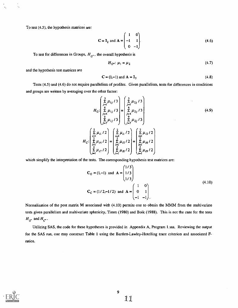
To test (4.5), the hypothesis matrices are:
[1 0
C=I2 andA= 1 1 .
0 1To test for differences in Groups, 1-1G. , the overall hypothesis is
and the hypothesis test matrices are
(4.6)
H /./3 = P2 (4.7)
C = (1,-1) and A = 13 (4.8)
Tests (4.5) and (4.6) do not require parallelism of profiles. Given parallelism, tests for differences in conditions
and groups are written by averaging over the other factor:
i 3 \ / 3I 111j / 3 E /12j / 3
i=1 i=16 6
HG: I pij /3 = E 112; /3 (4.9)j=4 j=4
9 9
I Pi/ /3 E Pzi / 30=7 / \,j=7 1
i 2 \ (2 \ / 2Z Ain / 2 Z pi' / 2 Z Ati3 / 2i=1 i=1 j=12 2 2
Z Pia / 2 = Z Pis / 2 = Z 11 i6 1 2i=1 i=1 i=12 2 2E iti7 / 2 I iiis / 2 I 1/0 / 2
i=1 ) i=1 ../ kJ-4 1
which simplify the interpretation of the tests. The corresponding hypothesis test matrices are:
H c:
11
/CG = (1,-1) and A = 1/ 3
1/3
1 0
Cc = (1/ 2,-1/ 2) and A= 0 1
1 1 .
(4.10)
Normalization of the post matrix M associated with (4.10) permits one to obtain the MMM from the multivariate
tests given parallelism and multivariate sphericity, Timm (1980) and Boik (1988). This is not the case for the tests
HG.
and H c.
Utilizing SAS, the code for these hypotheses is provided in Appendix A, Program 1.sas. Reviewing the output
for the SAS run, one may construct Table 1 using the Bartlett-Lawley-Hotelling trace criterion and associated F-
ratios.
9
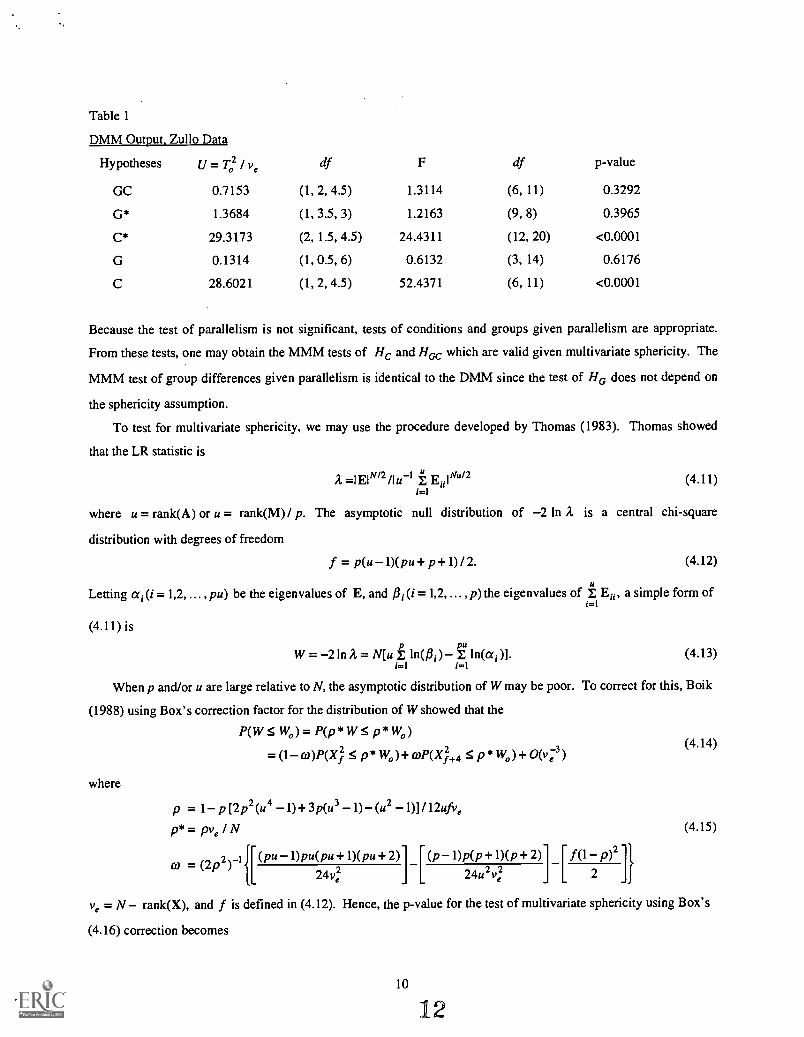
Table 1
DMM Output, Zullo Data
Hypotheses U = 02 / vo df F df p-value
GC 0.7153 (1, 2, 4.5) 1.3114 (6, 11) 0.3292
G* 1.3684 (1, 3.5, 3) 1.2163 (9, 8) 0.3965
C* 29.3173 (2, 1.5, 4.5) 24.4311 (12, 20) <0.0001
G 0.1314 (1, 0.5, 6) 0.6132 (3, 14) 0.6176
C 28.6021 (1, 2, 4.5) 52.4371 (6, 11) <0.0001
Because the test of parallelism is not significant, tests of conditions and groups given parallelism are appropriate.
From these tests, one may obtain the MMM tests of I 1 c and HGC which are valid given multivariate sphericity. The
MMM test of group differences given parallelism is identical to the DMM since the test of HG does not depend on
the sphericity assumption.
To test for multivariate sphericity, we may use the procedure developed by Thomas (1983). Thomas showed
that the LR statistic is
A =I EIN/2 /I u-1"
(4.11)i=i
where u = rank(A) or u = rank(M) / p. The asymptotic null distribution of 2 In A is a central chi-square
distribution with degrees of freedom
f = p(u-1)(pu+ p + 1) / 2. (4.12)
Letting a i(i = 1,2, ... , pu) be the eigenvalues of E, and Jai (i =1,2, , p) the eigenvalues of Eii, a simple form of1=1
(4.11) is
When
(1988) using
where
W = 21n A = N[u E ln(Pi) incam.i=1 1=1
p and/or u are large relative to N, the asymptotic distribution of W may be poor.
Box's correction factor for the distribution of W showed that the
P(W S WO= P(P * W 5 P * Wo)
= (1 co)P(Xj. 5 p* Wo)+ coP(4,4 5 p* Wo)+ 0(v:3)
p = 1 p [2 p2 (u4 1) + 3p(u3 1) (u2 1)] / 12ufve
p* = pve I N
1{[(puDpu(pu+1)(pu+ 2)1 +1)(p + 2)1
To correct for
f(1 p)2]}
(4.13)
this, Boik
(4.14)
(4.15)
[(p-1)p(p24v,2 24u 2 Ve2
[2
ve = N rank(X), and f is defined in (4.12). Hence, the p-value for the test of multivariate sphericity using Box's
(4.16) correction becomes
10
12
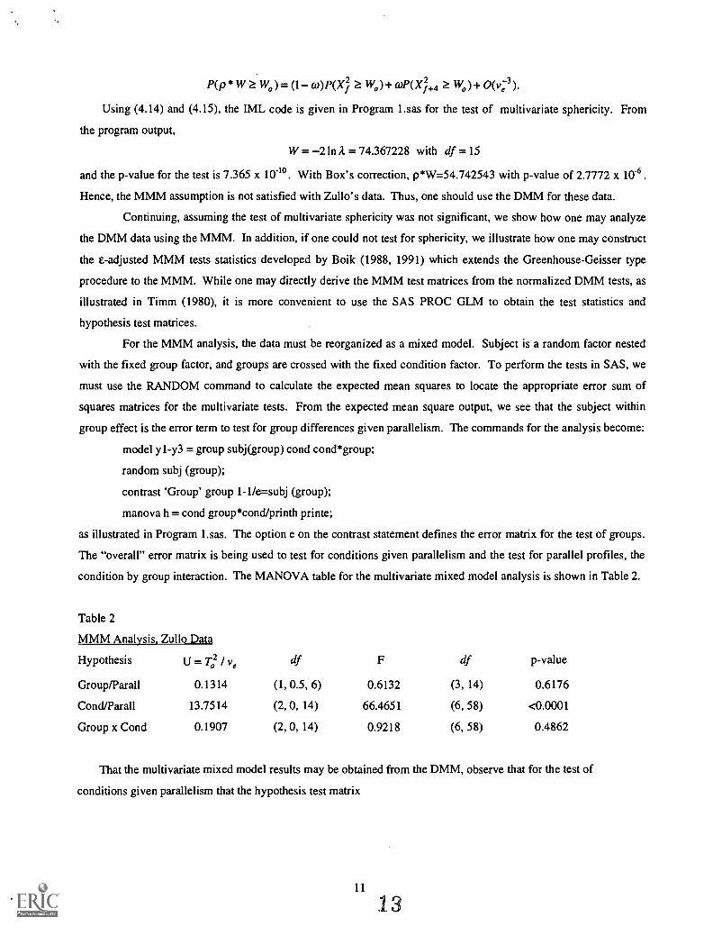
P(p * W Z Wo) = (1 co)P(4 Z WO+ oP(4,4 Z Wo) + 0(v:3 ).
Using (4.14) and (4.15), the IML code is given in Program 1.sas for the test of multivariate sphericity. From
the program output,
W = 21n = 74.367228 with df =15
and the p-value for the test is 7.365 x 10⁴°. With Box's correction, p*W=54.742543 with p-value of 2.7772 x 10⁻⁶.
Hence, the MMM assumption is not satisfied with Zullo's data. Thus, one should use the DMM for these data.
Continuing, assuming the test of multivariate sphericity was not significant, we show how one may analyze
the DMM data using the MMM. In addition, if one could not test for sphericity, we illustrate how one may construct
the c- adjusted MMM tests statistics developed by Boik (1988, 1991) which extends the Greenhouse-Geisser type
procedure to the MMM. While one may directly derive the MMM test matrices from the normalized DMM tests, as
illustrated in Timm (1980), it is more convenient to use the SAS PROC GLM to obtain the test statistics and
hypothesis test matrices.
For the MMM analysis, the data must be reorganized as a mixed model. Subject is a random factor nested
with the fixed group factor, and groups are crossed with the fixed condition factor. To perform the tests in SAS, we
must use the RANDOM command to calculate the expected mean squares to locate the appropriate error sum of
squares matrices for the multivariate tests. From the expected mean square output, we see that the subject within
group effect is the error term to test for group differences given parallelism. The commands for the analysis become:
model yl-y3 = group subj(group) cond cond*group;
random subj (group);
contrast 'Group' group 1-1/e=subj (group);
manova h = cond group*cond/printh printe;
as illustrated in Program 1.sas. The option e on the contrast statement defines the error matrix for the test of groups.
The "overall" error matrix is being used to test for conditions given parallelism and the test for parallel profiles, the
condition by group interaction. The MANOVA table for the multivariate mixed model analysis is shown in Table 2.
Table 2
MMM Analysis. Zullo Data
Hypothesis U= 02 /ye df F df p-value
Group/Parall 0.1314 (1, 0.5, 6) 0.6132 (3, 14) 0.6176
Cond/Parall 13.7514 (2, 0, 14) 66.4651 (6, 58) <0.0001
Group x Cond 0.1907 (2, 0, 14) 0.9218 (6, 58) 0.4862
That the multivariate mixed model results may be obtained from the DMM, observe that for the test of
conditions given parallelism that the hypothesis test matrix
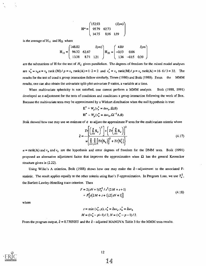
H* =
152.93 (Sym)
95.79 62.73
14.75 856 159
is the average of H11 and H22 where
'148.02 Sym) 4.89 Sym
H11 = 96.32 62.67 H22 = -053 0.06
13.38 8.71 1.21 1.36 -0.15 0.39
are the submatrices of H for the test of Hc given parallelism. The degrees of freedom for the mixed model analyses
are v: = vhu = vh rank (M) / p = vh rank(A) = 1.2 = 2 and v: = ye rank(M) / p = ye rank(A) = 16.6 / 3 = 32. The
results for the test of cond x group interaction follow similarly, Timm (1980) and Boik (1988). From the MMM
results, one can also obtain the univariate split-plot univariate F-ratios, a variable at a time.
When multivariate sphericity is not satisfied, one cannot perform a MMM analysis. Boik (1988, 1991)
developed an c- adjustment for the tests of conditions and conditions x group interaction following the work of Box.
Because the multivariate tests may be approximated by a Wishart distribution when the null hypothesis is true:
Es w(v: = Euve,Q,0)
11` Wp(v: = euvh,S2-IA,0)
Boik showed how one may use an estimate of 6 to adjust the approximate F tests for the multivariate criteria where
TrR Sii )21+ [Tr(ii1
Si=1 =
e = (4.17)
[Tr(Sy)]2 + TOO}a=1 j=1
u = rank(A) and vh and ve are the hypothesis and error degrees of freedom for the DMM tests. Boik (1991)
proposed an alternative adjustment factor that improves the approximation when SI has the general Kronecker
structure given in (2.22).
Using Wilks's A criterion, Boik (1988) shows how one may make the e- adjustment to the associated F-
statistic. The result applies equally to the other criteria using Rao's F-approximation. In Program 1.sas, we use To2,
the Bartlett-Lawley-Hotelling trace criterion. Then
F = 2(sN +1)7'02 I s2 (2 M + s + 1)(4.18)
F[s(2 M + s+ 1),2(sN + 1)]
where
s = min (vh,p), vh = euv v h = tuvh
M = (14 - p1-1)/ 2, N = (4 -p-1)/2.
From the program output, e = 0.7305055 and the e- adjusted MANOVA Table 3 for the MMM tests results.
12
14
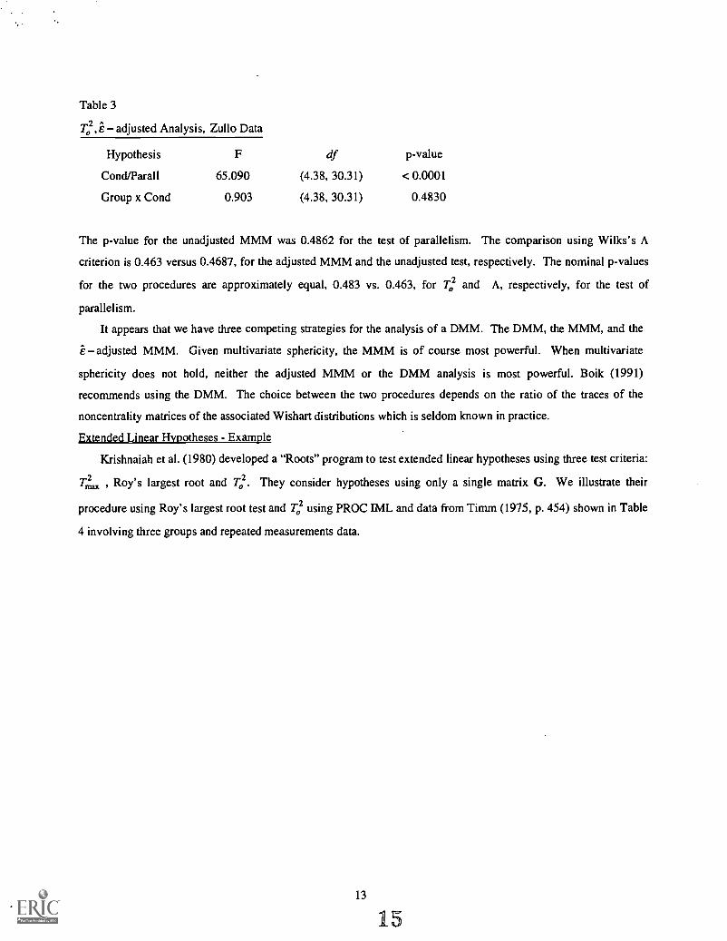
Table 3
T02, e adjusted Analysis, Zullo Data
Hypothesis F df p-value
Cond/Parall 65.090 (4.38, 30.31) < 0.0001
Group x Cond 0.903 (4.38, 30.31) 0.4830
The p-value for the unadjusted MMM was 0.4862 for the test of parallelism. The comparison using Wilks's A
criterion is 0.463 versus 0.4687, for the adjusted MMM and the unadjusted test, respectively. The nominal p-values
for the two procedures are approximately equal, 0.483 vs. 0.463, for To2 and A, respectively, for the test of
parallelism.
It appears that we have three competing strategies for the analysis of a DMM. The DMM, the MMM, and the
8 adjusted MMM. Given multivariate sphericity, the MMM is of course most powerful. When multivariate
sphericity does not hold, neither the adjusted MMM or the DMM analysis is most powerful. Boik (1991)
recommends using the DMM. The choice between the two procedures depends on the ratio of the traces of the
noncentrality matrices of the associated Wishart distributions which is seldom known in practice.
Extended Linear Hypotheses - Example
Krishnaiah et al. (1980) developed a "Roots" program to test extended linear hypotheses using three test criteria:
Tmax2 , Roy's largest root and 7;2. They consider hypotheses using only a single matrix G. We illustrate their
procedure using Roy's largest root test and 7;2 using PROC IML and data from Timm (1975, p. 454) shown in Table
4 involving three groups and repeated measurements data.
13
15
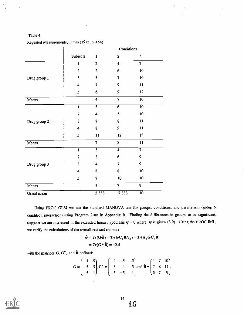
Table 4
Repeated Measurements, Timm (1975, p. 454)
Subjects 1
Conditions
2 3
1 2 4 7
2 2 6 10
Drug group 1 3 3 7 10
4 7 9 11
5 6 9 12
Means 4 7 10
1 5 6 10
2 4 5 10
Drug group 2 3 7 8 11
4 8 9 11
5 11 12 13
Means 7 8 11
1 3 4 7
2 3 6 9
Drug group 3 3 4 7 9
4 8 8 10
5 7 10 10
Means 5 7 9
Grand mean 5.333 7.333 10
Using PROC GLM we test the standard MANOVA test for groups, conditions, and parallelism (group x
condition interaction) using Program 2.sas in Appendix B. Finding the differences in groups to be significant,
suppose we are interested in the extended linear hypothesis w = 0 where w is given (3.9). Using the PROC IML,
we verify the calculations of the overall test and estimate
yi = Tr(Ge) = Tr(GColike)= Tr(A0GC0i1)
= Tr(G*11)= 2.5
with the matrices G, G*, and B defined:
1 .5 1 .5 .5 4 7 10
G = .5[ .5 , Ga = .5 1 .5 and a = 7 8 11
.5 1 .5 .5 1 5 7 9
.
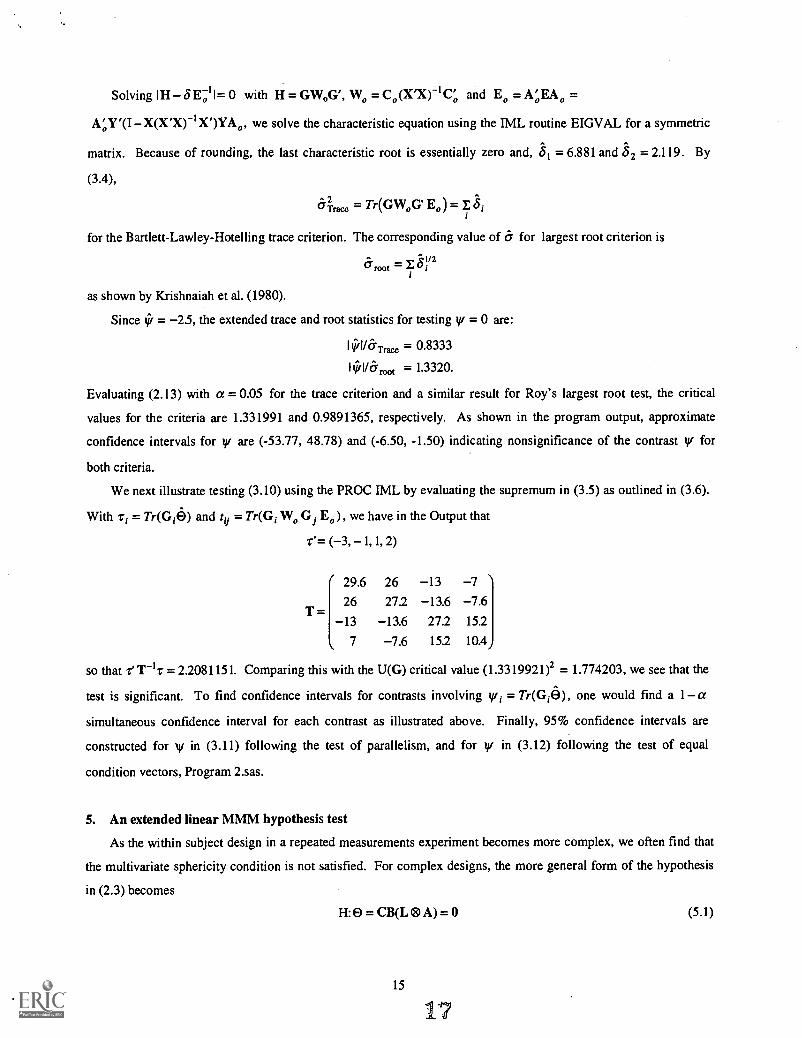
Solving IH 8 E;11= 0 with H = GW0G', Wo = Co (XX)-1C0 and Eo = A'oEiko =
X(X'X)-I X')YA0, we solve the characteristic equation using the IML routine EIGVAL for a symmetric
matrix. Because of rounding, the last characteristic root is essentially zero and, Sl = 6.881 and ;52 = 2.119. By
(3.4),
Trace = Tr(GW0G' Eo) = I
for the Bartlett-Lawley-Hotelling trace criterion. The corresponding value of o for largest root criterion is
&root = E ;"
as shown by Krishnaiah et al. (1980).
Since if = 23, the extended trace and root statistics for testing y/ = 0 are:
111/1/6-Trace = 0.8333
It//I /6,o°; = 1.3320.
Evaluating (2.13) with a = 0.05 for the trace criterion and a similar result for Roy's largest root test, the critical
values for the criteria are 1.331991 and 0.9891365, respectively. As shown in the program output, approximate
confidence intervals for 1,11 are (-53.77, 48.78) and (-6.50, -1.50) indicating nonsignificance of the contrast y/ for
both criteria.
We next illustrate testing (3.10) using the PROC IML by evaluating the supremum in (3.5) as outlined in (3.6).
With ri = Tr(Gie) and ty = Tr(GiWo Gi E0), we have in the Output that
r'= (-3, 1, 1, 2)
T=
( 29.6 26 13 7 \26 27.2 13.6 7.6
13 13.6 27.2 152
7 7.6 15.2 10.4
so that = 2.2081151. Comparing this with the U(G) critical value (1.3319921)2 = 1.774203, we see that the
test is significant. To find confidence intervals for contrasts involving y/i = Tr(Gie), one would find a 1 a
simultaneous confidence interval for each contrast as illustrated above. Finally, 95% confidence intervals are
constructed for yr in (3.11) following the test of parallelism, and for y/ in (3.12) following the test of equal
condition vectors, Program 2.sas.
5. An extended linear MMM hypothesis test
As the within subject design in a repeated measurements experiment becomes more complex, we often find that
the multivariate sphericity condition is not satisfied. For complex designs, the more general form of the hypothesis
in (2.3) becomes
H:e = CB(L ®A) = 0 (5.1)
15
17
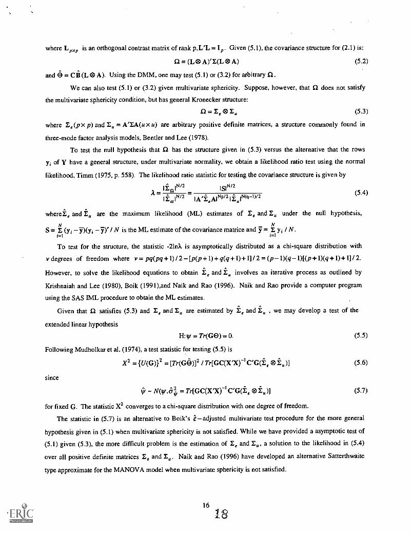
where Lp,p is an orthogonal contrast matrix of rank p,L'L = Ip. Given (5.1), the covariance structure for (2.1) is:
= (L 0 A)'E(L ®A) (5.2)
and e = CB (L 0 A). Using the DMM, one may test (5.1) or (3.2) for arbitrary S2.
We can also test (5.1) or (3.2) given multivariate sphericity. Suppose, however, that 12 does not satisfy
the multivariate sphericity condition, but has general Kronecker structure:
= Ee eiu (5.3)
where Ee (p x p) and Eu = A'EA(u x u) are arbitrary positive definite matrices, a structure commonly found in
three-mode factor analysis models, Bentler and Lee (1978).
To test the null hypothesis that S2 has the structure given in (5.3) versus the alternative that the rows
y, of Y have a general structure, under multivariate normality, we obtain a likelihood ratio test using the normal
likelihood, Timm (1975, p. 558). The likelihood ratio statistic for testing the covariance structure is given by
i 1N/2= =
I A'±eAINPI2 I Eu IN(q-1) /2(5.4)
whereE, and Eu are the maximum likelihood (ML) estimates of Ee and Eu under the null hypothesis,
N NS = E (y, y)(y1 3)' / N is the ML estimate of the covariance matrice and y = E y1 / N.
1=1 1 =1
To test for the structure, the statistic -210, is asymptotically distributed as a chi-square distribution with
v degrees of freedom where v= pq(pq +1) 12 [p(p + 1) + q(q +1)+1)12 = (p 1)(q 1)[(p +1)(q +1)+1)12.
However, to solve the likelihood equations to obtain Ee and Eu involves an iterative process as outlined by
Krishnaiah and Lee (1980), Boik (1991),and Naik and Rao (1996). Naik and Rao provide a computer program
using the SAS IML procedure to obtain the ML estimates.
Given that 12 satisfies (5.3) and Ee and Eu are estimated by Ee and Eu , we may develop a test of the
extended linear hypothesis
H: = Tr(Ge) = 0.
Following Mudholkar et al. (1974), a test statistic for testing (5.5) is
X2 = {U(G)}2 = [Tr(G6)]2 / Tr[GC(X'X)-i C'G(Ee Eu
since
(5.5)
(5.6)
AlOy,&21if = Tr[GC(X'X)-i CG(Ee E)] (5.7)
for fixed G. The statistic X2 converges to a chi-square distribution with one degree of freedom.
The statistic in (5.7) is an alternative to Boik's adjusted multivariate test procedure for the more general
hypothesis given in (5.1) when multivariate sphericity is not satisfied. While we have provided a asymptotic test of
(5.1) given (5.3), the more difficult problem is the estimation of Ee and Eu, a solution to the likelihood in (5.4)
over all positive definite matrices Ee and Eu. Naik and Rao (1996) have developed an alternative Satterthwaite
type approximate for the MANOVA model when multivariate sphericity is not satisfied.
References
Amemiya, Y. (1994). On multivariate mixed model analysis. In T. W. Anderson, K. T. Fang, & I. Olkin (Eds.)Multivariate Analysis and Its Applications, IMS Lecture Notes, Volume 24, 83-95. IMS: Hayward, CA.
Bent ler, P. M. & S. Y. Lee (1978). Statistical analysis of a three-mode factor analysis model. Psychometrika, 43,343-352.
Boik, R. J. (1988). The mixed model for multivariate repeated measures: Validity conditions and an approximatetest. Psychometrika, 53, 469-486.
Boik, R. J. (1991). Scheffe's mixed model for multivariate repeated measures a relative efficiency evaluation.Communications in Statistics, A20, 1233-1255.
Boik, R. J. (1993). The analysis of two-factor interactions in fixed effects linear models. Journal of EducationalStatistics, 18, 1-40.
Bradu, D. & K. D. Gabriel (1974). Simultaneous statistical inference on interactions in two-way analysis ofvariance. Journal of the American Statistical Association, 69, 428-436.
Diggle, P.J., K.Y. Liang. and S.L. Zeger (1994). Analysis of longitudinal data. Oxford: Oxford University Press.
Graham, A. (1981). Kronecker products and matrix calculus: With applications, New York: Wiley.
Hecker, H. (1987). A generalization of the GMANOVA-model. Biometrical Journal, 29, 763-790.
Krishnaiah, P. R. & J. C. Lee (1980). Likelihood ratio tests for mean vectors and covariance matrices. In P. R .Krishnaih (Ed.) Handbook of Statistics, Analysis of Variance, Volume I, 513-570. New York: North-Holland.
Krishnaiah, P. R., G. S. Mudholkar, & P. Subbaiah (1980). Simultaneous test procedures for mean vectors andcovariance matrices. In P. R. Krishnaih (Ed.) Handbook of Statistics, Analysis of Variance, Volume I, 631-672. New York: North-Holland.
Lindsey, J. K. (1993). Models for repeated measurements. Oxford: Oxford University Press.
Longford, N. T. (1993). Random coefficient models. Oxford: Oxford University Press.
Mudholkar, G. S., M. L. Davidson & P. Subbaiah (1974). Extended linear hypotheses and simultaneous tests inmultivariate analysis of variance, Biometrika, 61, 467-477.
Muller, K. E., L.M. La Vange, S.L. Ramey, & E. T. Ramey (1992). Power calculations for general linearmultivariate models including repeated measures applications. Journal of the American Statistical
Association, 87, 1209-1226.
Naik, D. N. and S. S. Rao (1996). Analysis of multivariate repeated measurements (unpublished manuscript, Dept.of Mathematics and Statistics, Old Dominion University).
Pillai, K.C.S. (1960). Statistical Tables for Tests of Multivariate Hypotheses. Manila: Statistical Center,University of Philippines.
Pillai, K.C.S., and D.L. Young (1971). On the exact distribution fo Hotelling's generalized Toe, Journal ofMultivariate Analysis, 1, 90-107.
17
Potthoff, R.F. and S.N. Roy (1964). A generalized multivariate analysis of variance model useful especially forgrowth curve problems. Biometrika, 51, 313-326.
Reinsel, G. (1982). Multivariate repeated-measurement or growth curve models with multivariate random-effectscovariance structure. Journal of the American Statistical Association, M 190-195.
SAS (1990). SAS/STAT User's Guide, Version 6, (4th ed.), Vol. 1. Cary, NC: SAS Institute, Inc.
Seber, G.A. F. (1984). Multivariate Observations. New York: John Wiley.
Thomas, D. R. (1983). Univariate repeated measures techniques applied to multivariate data. Psychometrika, 48,451-464.
Timm, N. H. (1980) Multivariate analysis of variance of repeated measurements. In P. R. Krishnaiah (Ed.)Handbook of Statistics, Analysis of Variance, Volume I, 41-87. New York: North Holland.
Timm, N. H. (1975). Multivariate analysis with application in education and psychology. Monterey, CA: BrooksCole. [Reprinted by the Digital Printshop, 528 East Lorain Street., Oberlin, OH 44074 ISBN 0-7870-0008-6]
von Rosen, D. (1991). The growth curve model: A review. Communications in Statistics, 20, 2791-2822.
18 20
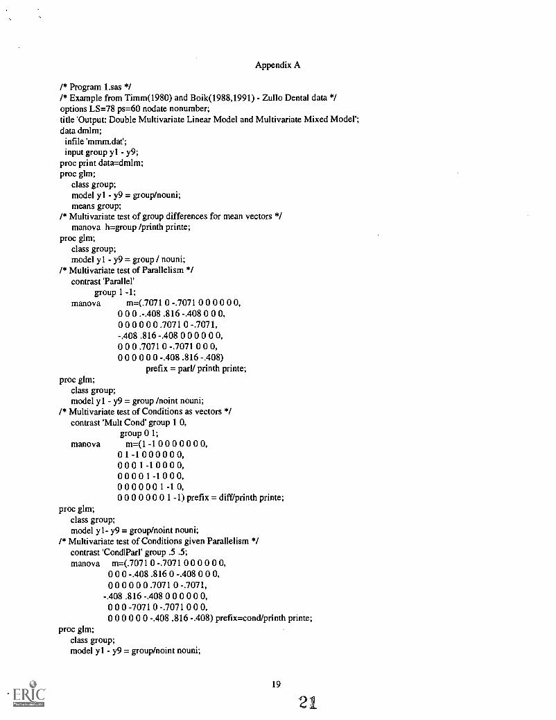
Appendix A
/* Program 1.sas *//* Example from Timm(1980) and Boik(1988,1991) Zullo Dental data */options LS=78 ps=60 nodate nonumber;title 'Output: Double Multivariate Linear Model and Multivariate Mixed Model';data dmlm;
infile 'mmm.dat';input group yl - y9;
proc print data =dmlm;proc glm;
class group;model yl - y9 = group/nouni;means group;
/* Multivariate test of group differences for mean vectors */manova h=group /printh printe;
proc glm;class group;model yl - y9 = group / nouni;
/* Multivariate test of Parallelism */contrast 'Parallel'
group 1 -1;manova m=(.7071 0 -.7071 0 0 0 0 0 0,
0 0 0. -.408 .816 -.408 0 0 0,0 0 0 0 0 0 .7071 0 -.7071,-.408 .816 -.408 0 0 0 0 0 0,0 0 0.7071 0- .7071 0 0 0,0 0 0 0 0 0 -.408 .816 -.408)
prefix = parl/ printh printe;proc glm;
class group;model yl - y9 = group /noint nouni;
/* Multivariate test of Conditions as vectors */contrast 'Mult Cond' group 1 0,
group 0 1;manova m.(1 -1 0 0 0 0 0 0 0,
0 1 -1 0 0 0 0 0 0,000 1 -1 0 0 0 0,0 0 0 0 1 -1000,0 0 0 0 0 0 1 -1 0,0 0 0 0 0 0 0 1 -1) prefix = diff/printh printe;
proc glm;class group;model yl- y9 = group/noint nouni;
/* Multivariate test of Conditions given Parallelism */contrast 'CondlParl' group .5 .5;manova m=(.7071 0 -.7071 0 0 0 0 0 0,
0 0 0 -.408 .816 0 -.408 0 0 0,0 0 0 0 0 0 .7071 0 -.7071,
-.408 .816 -.408 0 0 0 0 0 0,0 0 0- 7071 0 -.7071 0 0 0,0 0 0 0 0 0 -.408 .816 -.408) prefix=cond/printh printe;
proc glm;class group;model yl - y9 = group/noint nouni;
19
21
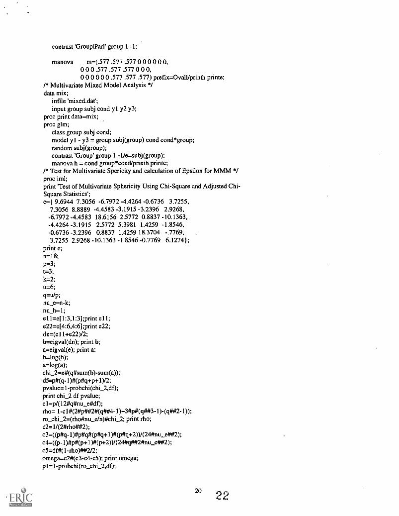
contrast 'Group1Parl' group 1 -1;
manova m=(.577 .577 .577 0 0 0 0 0 0,0 0 0 .577 .577 .577 0 0 0,0 0 0 0 0 0.577 .577 .577) prefix=Ovall/printh printe;
/* Multivariate Mixed Model Analysis */data mix;
infile 'mixed.dat;input group subj cond yl y2 y3;
proc print data=mix;proc glm;
class group subj cond;model yl - y3 = group subj(group) cond cond*group;random subj(group);contrast 'Group' group 1 -1/e=subj(group);manova h = cond group*cond/printh printe;
/* Test for Multivariate Spericity and calculation of Epsilon for MMM */proc iml;print 'Test of Multivariate Sphericity Using Chi-Square and Adjusted Chi-Square Statistics;e=( 9.6944 7.3056 -6.7972 -4.4264 -0.6736 3.7255,
7.3056 8.8889 -4.4583 -3.1915 -3.2396 2.9268,-6.7972 -4.4583 18.6156 2.5772 0.8837 -10.1363,-4.4264 -3.1915 2.5772 5.3981 1.4259 -1.8546,-0.6736 -3.2396 0.8837 1.4259 18.3704 -.7769,3.7255 2.9268 -10.1363 -1.8546 -0.7769 6.1274);
print e;n=18;
P=3;t=3;k=2;u=6;q =u/p;nu_e=n-k;nu_h=1;ell=e[1:3,1:3];print ell;e22=e[4:6,4:6];print e22;dn=(ell+e22)/2;b=eigval(dn); print b;a=eigval(e); print a;b=log(b);a=log(a);chi_2=n#(q#sum(b)-sum(a));df=p#(q-1)#(p#q+p+1)/2;pvalue=1-probchi(chi_2,d0;print chi_2 df pvalue;cl=p/(12#q#nu_e#df);rho= 1-cl#(2#p4t#2#(q##4-1)+3#p#(q##3-1)-(q##2-1));ro_chi_2=(rho#nu_e/n)#chi_2; print rho;c2=1/(2#rholi4t2);c3=((p#q-1)4tp#q#(pitq+1)#(p#q+2))/(24#nu_e##2);c4=((p-1)4tp#(p+1)#(p+2))/(24#q##2#nu_e#4#2);c5=df#(1-rho)##2/2;omega=c2#(c3-c4-c5); print omega;p1=1-probchi(ro_chi_2,d0;
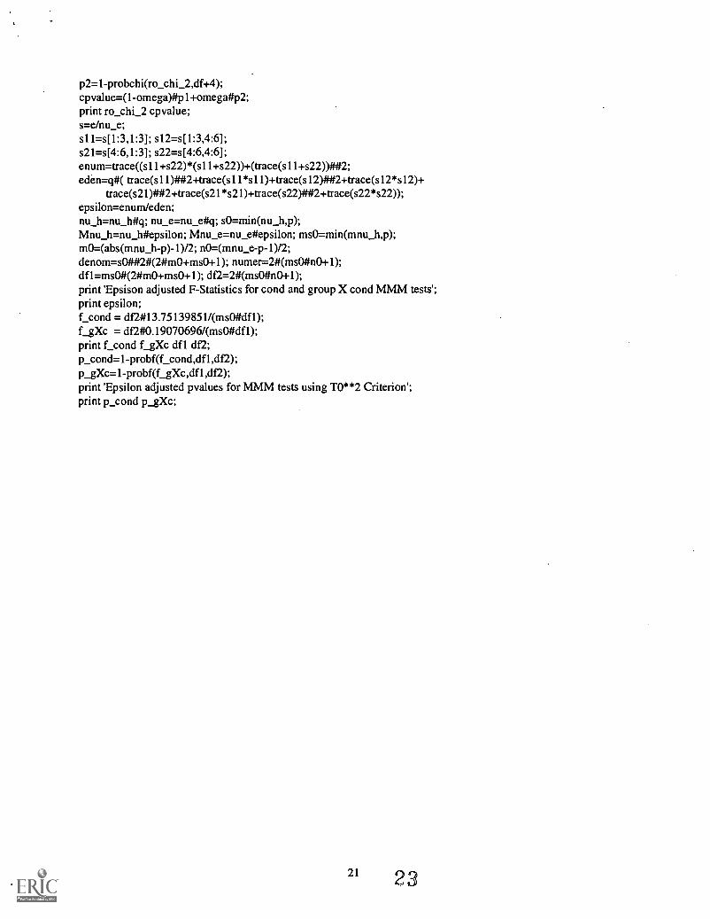
p2=1-probchi(ro_chi_2,df+4);cpvalue=(1-omega)#pl+omegaltp2;print ro_chi_2 cpvalue;s=e/nu_e;sll=s[1:3,1:3]; s12=s[1:3,4:6];s21=s[4:6,1:3]; s22=s[4:6,4:6];enum=trace((sll+s22)*(s11+s22))+(trace(s11+s22))#42;eden=q#( trace(s11)##2+trace(sll*s11)+trace(s12)##2+trace(s12*s12)+
trace(s21)##2+trace(s21*s21)+trace(s22)##2+trace(s22*s22));epsilon=enum/eden;nu_h=nu_h#q; nu_e=nu_e#q; s0=min(nu_h,p);Mnu_h=nu_h#epsilon; Mnu_e=nu_e#epsilon; ms0=min(mnu_h,p);m0=(abs(mnu_h-p)-1)/2; n0=(mnu_e-p-1)/2;denom=s0##2#(2#m0+ms0+1); numer=2#(ms0#n0+1);dfl=ms0#(2#m0+ms0+1); df2=2#(ms0#n0+1);print 'Epsison adjusted F-Statistics for cond and group X cond MMM tests';print epsilon;f cond = df2#13.75139851/(ms0#dfl);f_gXc = df2#0.19070696/(ms0#df1);print f cond f_gXc dfl df2;p_cond=l-probf(f cond,dfl,df2);p_gXc=1-probf(f_gXc,dfl,df2);print 'Epsilon adjusted pvalues for MMM tests using TO**2 Criterion;print p_cond p_gXc;
21 23
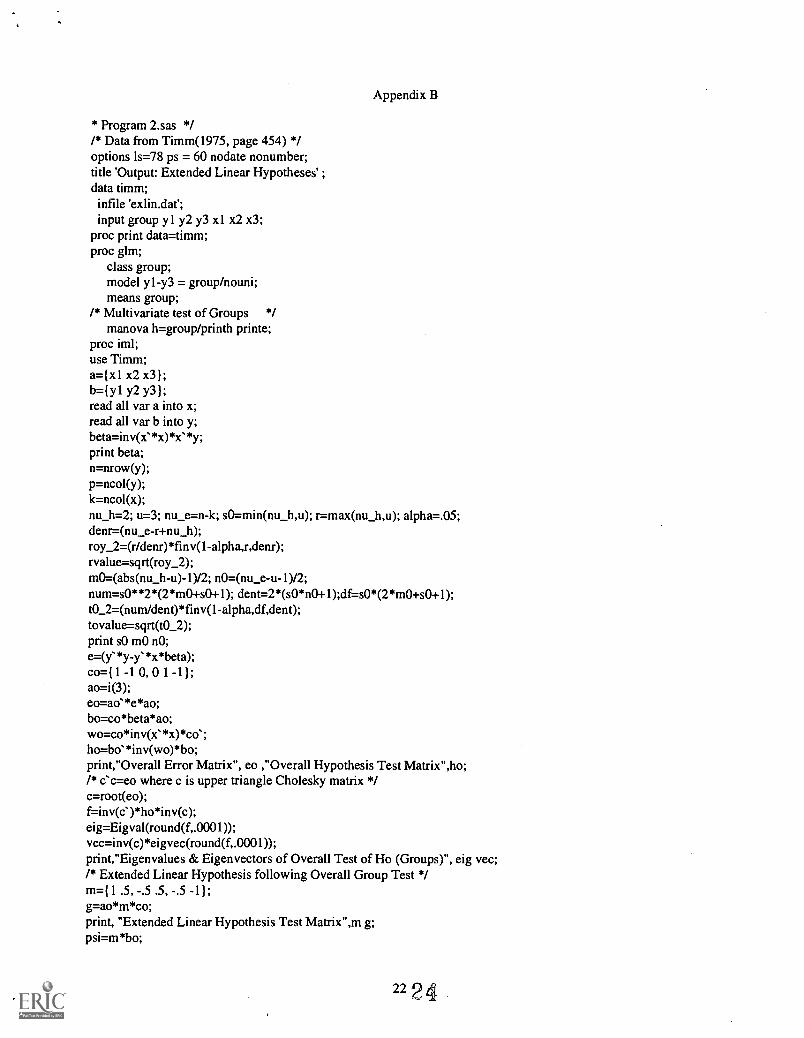
Appendix B
* Program 2.sas *//* Data from Timm(1975, page 454) */options ls=78 ps = 60 nodate nonumber;title 'Output: Extended Linear Hypotheses' ;data timm;
infile 'exlin.dat;input group yl y2 y3 xl x2 x3;
proc print data=timm;proc glm;
class group;model yl-y3 = group/nouni;means group;
/* Multivariate test of Groups */manova h=group/printh printe;
proc iml;use Timm;a={xl x2 x3};b = {yl y2 y3};read all var a into x;read all var b into y;beta=inv(xs*x)*xs*y;print beta;n=nrow(y);p=ncol(y);k=ncol(x);nu_h=2; u=3; nu_e=n-k; s0=min(nu_h,u); r=max(nu_h,u); alpha=.05;denr=(nu_e-r+nu_h);roy_2=(r/denr)*finv(1-alpha,r,denr);rvalue=sqrt(roy_2);m0.(abs(nu_h-u)-1)12; n0=(nu_e-u-1)/2;num=s0**2*(2*m0+s0+1); dent=2*(s0 *n0+1);df=s0*(2*m0+s0+1);t0_2=(num/dent)*finv(1-alpha,df,dent);tovalue=sqrt(t0_2);print sO m0 n0;e=(y'*y-ys*x*beta);co={ 1 -1 0, 0 1 -1 };ao=i(3);eo=aos*e*ao;bo=co*beta*ao;wo=co*inv(x'*x)*cos;ho=bo'*inv(wo)*bo;print,"Overall Error Matrix", eo ,"Overall Hypothesis Test Matrix",ho;/* c'c=eo where c is upper triangle Cholesky matrix */c=root(eo);f=inv(cs) *ho*inv(c);eig=Eigval(round(f,.0001));vec=inv(c) *eigvec(round(C.0001));print,"Eigenvalues & Eigenvectors of Overall Test of Ho (Groups)", eig vec;/* Extended Linear Hypothesis following Overall Group Test */m={ 1 .5, -.5 .5, -.5 -1};g=ao*m*co;print, "Extended Linear Hypothesis Test Matrix",m g;psi=m*bo;
2224

psi_hat=trace(psi);tr_psi=abs(psi_hat);h=m*wo*ms;eo=inv (eo);c=root(eo);f= inv(c') *h *inv(c);xeig=Eigval(round(f,.0001));print, "Eigenvalues of Extended Linear Hypothesis", xeig;to_2=tr_psi/sqrt(sum(xeig)); print, "Extended To**2 Statistic", to_2;print, "Extended To**2 Critical Value", tovalue;root=tr_psi/sum(ssq(xeig)); print, "Extended Largest Root Statistic", root;print, "Extended Largest Root Critical Value", rvalue;print psi_hat alpha;ru=psi_hat+rvalue*sum(ssq(xeig));rl=psi_hat-rvalue*sum(ssq(xeig));vu=psi_hat+tovalue*sqrt(sum(xeig));vl=psi_hat-tovalue *sqrt(sum(xeig));print 'Approximate Simultaneous Confidence Intervals;print 'Contrast Significant if interval does not contain zero;print 'Extended Root interval: ('rl ru ')';print 'Extended Trace interval: ('vl vu ')';/* Multiple Extended Linear Hypothesis using To**2 */m1={ 1 0,0 0,0 0}; m2={0 0,1 0,0 0}; m3={0 0,0 1,0 0}; m4={0 0,0 0,0 1};print,"Multiple Extended Linear Hypothesis Test Matrices", ml,m2,m3,m4;gl=ao*ml*co; g2=ao*m2*co; g3=ao*m3*co; g4=ao*m4*co;tl=trace(m1*bo); t2=trace(m2*bo); t3=trace(m3*bo); t4=trace(m4*bo);tau=t1//t2//t3//t4;tl 1=trace(ml*wo*mr*eo);t21=trace(m2*wo*m1'*eo); t22=trace(m2*wo*m2s*eo);t31=trace(m3*wo*m1s*eo); t32=trace(m3*wo*m2'*eo); t33=trace(m3*wo*m3s*eo);t41=trace(m4*wo*m1'*eo); t42=trace(m4*wo*m2**eo); t43=trace(m4*wo*m3s*eo);t44=trace(m4*wo*m4s*eo);r1=t1111t2111t3111t41;
r2=t2111t2211t3211t42;
r3=t3111t3211t3311t43;
r4=t4111t4211t4311t44;
t=r1//r2//r3//r4;print tau,t;to_4=tau'*inv(t)*tau;print, "Extended Linear Hypothesis Criterion To**2 Squared", to_4;print, "Extended To**2 Critical Value", t0_2;/* Multivariate test of Parallelism */data timm;infile 'exlin.dat;input group yl y2 y3 xl x2 x3;
proc glm;class group;model yl-y3 = group/nouni;manova h = group m = ( 1 -1 0,
0 1 -1) prefix = diff/printe printh;proc iml;use Timm;a={x1 x2 x3 };b = {yl y2 y3};read all var a into x;
23 25
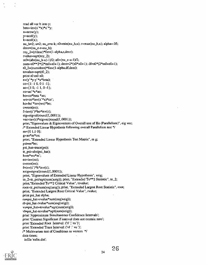
read all var b into y;beta=inv(xs*x)*xs*y;n=nrow(y);p=ncol(y);k=ncol(x);nu_h=2; u=2; nu_e=n-k; s0=min(nu_h,u); r=max(nu_h,u); alpha=.05;denr=(nu_e-r+nu_h);roy_2=(r/denr)*finv(1-alpha,r,denr);rvalue=sqrt(roy_2);m0=(abs(nu_h-u)-1)/2; n0=(nu_e-u-1)/2;num=s0**2*(2*m0+s0+1); dent=2*(sO*n0+1); df=s0*(2*m0+s0+1);t0_2=(nurn/dent) *finv(1-alpha,dfident);tovalue=sqrt(t0_2);print sO m0 n0;e=(ys*y-y'*x*beta);co =(1 -1 0, 0 1 -1);ao=(1 0, -1 1, 0 -1);eo=aos*e*ao;bo=co*beta *ao;wo=co*inv(xs*x)*cos;ho=bo'*inv(wo)*bo;c=root(eo);f= inv(c') *ho *inv(c);eig=eigval(round(f,.0001));vec=inv(c)*eigvec(round(f,.0001));print,"Eigenvalues & Eigenvectors of Overall test of Ho (Parallelism)", eig vec;/* Extended Linear Hypothesis following overall Parallelism test */m =(01,1 01;g=ao*m*co;print, "Extended Linear Hypothesis Test Matrix", m g;psi=m*bo;psi_hat=trace(psi);tr_psi=abs(psi_hat);h=m*wo*ms;eo=inv(eo);c=root(eo);f= inv(c') *h *inv(c);xeig=eigval(round(f,.0001));print, "Eigenvalues of Extended Linear Hypothesis", xeig;to_2=tr_psi/sqrt(sum(xeig)); print, "Extended To**2 Statistic", to_2;print,"Extended To**2 Critical Value", tovalue;root=tr_psi/sum(ssq(xeig)); print, "Extended Largest Root Statistic", root;print, "Extended Largest Root Critical Value", rvalue;print psi_hat alpha;ru=psi_hat+rvalue*sum(ssq(xeig));rl=psi_hat-rvalue*sum(ssq(xeig));vu=psi_hat+tovalue*sqrt(sum(xeig));vl=psi_hat-tovalue*sqrt(sum(xeig));print 'Approximate Simultaneous Confidence Intervals;print 'Contrast Significant if interval does not contain zero;print 'Extended Root Interval: ('rl ru ');print 'Extended Trace Interval: ('vl vu ') ;/* Multivariate test of Conditions as vectors */data timm;
infile 'exlin.dat';
2624

input group yl y2 y3 xl x2 x3;proc glm;
class group;model yl-y3 = group/noint nouni;contrast 'Mult Cond' group 1 0 0,
group 0 1 0,group 0 0 1;
manova m=(1 -1 0,0 1 -1) prefix = diff/ prince printh;
proc iml;use timm;a={xl x2 x3};b = {yl y2 y3);read all var a into x;read all var b into y;beta=inv(x'*x)*xs*y;n=nrow(y);p=ncol(y);k=ncol(x);nu_h=3; u=2; nu_e=n-k; s0=min(nu_h,u); r=max(nu_h,u); alpha=.05;denr=(nu_e-r+nu_h);roy_2=(r/denr)*finv(1-alpha,r,denr);rvalue=sqrt(roy_2);m0Mabs(nu_h-u)-1)/2; n0=(nu_e-u-1)/2;num=s0**2*(2*m0+s0+1); dent=2*(sO*n0+1); df=s0*(2*m0+s0+1);t0_2=(num/dent)*finv(1-alpha,df,dent);tovalue=sqrt(t0_2);print sO m0 n0;e=(y'*y-y'*x*beta);co=i(3);ao={1 0, -1 1,0-1);eo=aos*e*ao;bo=co*beta*ao;wc=co*inv(x'*x)*cos;ho=bo'*inv(wo)*bo;c=root(eo);f=inv(cs)*ho*inv(c);eig=eigval(round(f,.0001));vec=inv(c)*eigvec(round(f,.0001));print, "Eigenvalues & Eigenvectors of Overall test of Ho (Conditions)", eig vec;m=11 0 1, 0 1 1);g=ao*m*co;print, "Extended Linear Hypothesis Test Matrix", m g;psi=m*bo;psi_hat=trace(psi);tr_psi=abs(psi_hat);h=m*wo*m ;eo=inv(eo);c=root(eo);f= inv(c') *h *inv(c);xeig=eigval(round(f,.0001));print, "Eigenvalues of Extended Linear Hypothesis", xeig;to_2=tr_psi/sqrt(sum(xeig)); print, "Extended To**2 Statistic", to_2;print, "Extended TO**2 Critical Value", tovalue;root= trpsi/sum(ssq(xeig)); print, "Extended Largest Root Statistic", root;

print, "Extended Largest Root Critical Value", rvalue;print psi_hat alpha;ru=psi_hat+rvalue*sum(ssq(xeig));rl=psi_hat-rvalue *sum(ssq(xeig));vu=psi_hat+tovalue*sqrt(sum(xeig));vl=psi_hat-tovalue*sqrt(sum(xeig));print 'Approximate Simultaneous Confidence Intervals;print 'Contrast Significant if interval does not contain zero';print 'Extended Root Interval: ('rl ru ')';print 'Extended Trace Interval: ('vl vu ')';
I.
U.S. DEPARTMENT OF EDUCATIONOffice of Educational Research and Improvement (OERI)
Educational Resources Information Center (ERIC)
REPRODUCTION RELEASE(Specific Document)
DOCUMENT IDENTIFICATION:
Title:
Full Rank Multivariate Repeated Measurement Designs and Extended LinearHypotheses
Author(s):Neil H. Timm
Corporate Source:
University of Pittsburgh
Publication Date:
October 1, 1996
II. REPRODUCTION RELEASE:
Fri
In order to disseminate as widely as possible timely and significant materials of interest to the educational community, documentsannounced in the monthly abstract journal of the ERIC system, Resources in Education (RIE), are usually made available to usersin microficne, reproduced paper copy, and electronidoptical media, and sold through the ERIC Document Reproduction Service(EDRS) or other ERIC vendors. Credit is given to the source of each document, and, if reproduction release is granted, one of thefollowing notices is affixed to the docuMent.
If permission is granted to reproduce the identified document, please CHECK ONE of the following options and sign the releasebelow.
4. Sample sticker to be affixed to document Sample sticker to be affixed to document 11*
Check herePermittingmicrofiche(4" x 6" film),paper copy,electronic, andoptical mediareproduction.
"PERMISSION TO REPRODUCE THISMATERIAL HAS BEEN GRANTED BY
C7CN>
TO THE EDUCATIONAL RESOURCESINFORMATION CENTER (ERIC)*
Level 1
"PERMISSION TO REPRODUCE THISMATERIAL IN OTHER THAN PAPER
COPY HAS BEEN GRANTED BY
SaTO THE EDUCATIONAL RESOURCES
INFORMATION CENTER (ERIC)"
Level 2
or here
Permittingreproductionin other thanpaper copy.
Sign Here, PleaseDocuments will be processed as indicated provided reproduction quality permits. If permission to reproduce is granted, but
neither box is checked, documents will be processed at Level 1.
"I hereby grant to the Educational Resources Information Center (ERIC) nonexclusive permission to reproduce this document asindicated above. Reproduction from the ERIC microfiche or electronic /optical media by persons other than ERIC employees and itssystem contractors requires permission from the copyright holder. Exception is made for non-profit reproduction by libraries and other
service agencies atisfy information needs of educators in response to discrete inquiries."
Signature: .....e./y ----- Position:Professor
Printed Name:Neil H. Timm
Organization:University of Pittsburgh
Address:Dept. of Psychology in Education5C01 Forbes QuadranglePittsburgh, PA 15260
Telephone Number: /l412 )624-7233
Date:October 1, 1996
OVER

