Embed Size (px)
Citation preview

DOCUMENTOS DE ECONOMÍA Y FINANZAS INTERNACIONALES
Working Papers on International
Economics and Finance
DEFI 10-06 September 2010
Bilateral trade flows and income-
distribution similarity
Inmaculada Martínez-Zarzoso Sebastian Vollmer
Asociación Española de Economía y Finanzas Internacionales
www.aeefi.com ISSN: 1696-6376

1
Bilateral Trade Flows and Income-Distribution
Similarity
Inmaculada Martínez-Zarzoso a)
Georg-August University of Göttingen and University Jaume I
Sebastian Vollmer b)
Harvard University and University of Hannover
Abstract
This paper accounts for non-homothetic preferences by specifically investigating the role
of income per capita and income-distribution differences in the context of the gravity
model of trade. A theoretically justified gravity model is estimated for disaggregated
trade data using a sample of 104 exporters and 108 importers for 1980-2003 to achieve
two main goals. First we are able to empirically test some of the theoretical predictions of
Markusen (2010), namely that there is a positive dependence of trade on per capita
income and that higher inequality increase trade of more sophisticated goods. Second,
and in line with the Linder hypothesis, we hypothesized that a higher demands’ overlap
implies a more similar demand structure and therefore more trade. We test this hypothesis
with new measures of income-distribution similarity. National income distributions are
used to calculate income similarity indices that measure how much each country pair
overlaps in terms of income distribution and population. We find that per capita income is
positively related to bilateral trade and that on average, a 10 percent increase in income-
distribution similarities increases exports by almost 4 percent being this effect stronger
for more sophisticated goods in comparison with more homogenous ones.
JEL classification: F10, F14, D31
Keywords: exports; income distribution; gravity equation; density estimation; non-homothetic
preferences.
a)
Financial support from the Spanish Ministry of Science and Technology is grateful acknowledged (SEJ
2007-67548). E-mail: [email protected]. b)
Email: [email protected].

2
Bilateral Trade Flows and Income-Distribution
Similarity 1. Introduction
The role of within country income distributions and between country income-distribution
similarities has been a relatively neglected area in international trade. Most trade theories
assumed that preferences are homothetic and identical across countries, giving a very small
role to demand patterns as factors that can explain international trade. This assumption might
have been useful to simplify the modeling framework, but it was based on no or only a weak
empirical foundation. Tastes cannot be considered identical for all consumers in a country;
studies clearly find consumer preferences to be non-homothetic (Hunter and Markusen, 1988;
Hunter, 1991).
An early exception to the main strand of theoretical models is the well-known Linder
hypothesis (Linder, 1961). He departs from traditional trade theory where supply side factors
are the main determinants of trade. He argued that the traditional theories cannot explain why
countries would engage in both exports and imports of the same type of products. He
considers that demand for a product has to appear first in the producer country and that then
this product can be exported to other countries that have similar demand structures.
Recently, Fajgelbaum et al. (2009), Fieler (2009) and Markusen (2010) incorporated the
assumption of non-homothetic consumer preferences in general models of international trade.
Markusen (2010) builds a generic model of identical but non-homothetic preferences and
presents a unified and testable set of results. The attractiveness of the model lies on its
simplicity without lack of generality and its predictions that also apply to imperfect
competition and increasing returns to scale.
With respect to the related empirical literature, we find several studies that tried to test
the Linder hypothesis obtaining mixed results. These are summarized in McPherson, Redfearn

3
and Tieslau (2000, 2001). In most cases a gravity framework was used and differences in
income per capita is the variable selected to measure income similarities between trading pairs
(Arnon and Weinblatt, 1988; Arad and Hirsch, 1981; Choi, 2002; Martínez-Zarzoso and
Nowak-Lehmann, 2004). Hallak (2010) focuses on product quality and shows that the failure
to confirm the Linder hypothesis in past studies could be due to aggregation bias. He finds
support for the Linder hypothesis by testing different type of products separately.
Most of the abovementioned studies consider per capita income differences between
countries. Instead, a few recent studies considered the within country distribution of income
as a determinant of bilateral trade flows. Hunter (1991), Francois and Kaplan (1996),
Matsuyama (2000) and Mitra and Trindade (2005); Bohman and Nilsson (2007), Chul Choi et
al. (2009) are some of them.
The purpose of this paper is twofold. First, we aim to test some of the theoretical
predictions derived in Markusen (2010), specifically the role played by income per capita in
gravity equations and the effect of within country income inequality on trade. Second we
estimate the effect of between country income-distribution similarities on bilateral trade. To
our knowledge this relationship has not been jet investigated and the theoretical foundations
are also missing. Therefore we suggest an avenue for further theoretical research. We
accomplish our second aim by providing a simple measure of similarity of demand structures
between countries that uses information of within country distribution of income. To construct
the index, we first estimate the distribution of income within each country of the world and
then we measure to what extent the distributions of two given countries overlap. The
underlying assumption is that the overlap between the respective density functions of income
within each country can be considered as a good proxy for the overlapping demand structure
between trading partners. Bertola, Foellmi and Zweimüller (2006) developed a framework for
analyzing non-homothetic demand, which illustrates the assumptions behind our proposed
method. The proposed measure is added as explanatory variable in a gravity model of trade.

4
The results from estimating the theoretically justified gravity model of trade show a positive
effect of income per capita on bilateral trade, holding constant aggregate income and a
significant and economically important effect of similarity of demand structures (measured by
the overlap of income distributions) on bilateral disaggregated trade flows.
In the next Section we explain how to construct the measure for income distribution
similarity. In Section 3 we conduct our empirical analysis and present the main results, before
concluding in Section 4.
2. Income-distribution overlaps between countries
We propose three different measures of demand similarity for each pair of countries
based on their income distributions. National income distributions are derived from two main
data sources. Income data are drawn from the Penn World Tables 6.2 (Heston, Summers and
Aten, 2006), which report the real GDP per capita in constant international dollars (chain
series, base year 2000), available for most countries. However, for three particularly populous
countries namely, Bangladesh, Russia and Ukraine we estimated the initial missing values1.
Our second data source is the inequality dataset proposed by Grün and Klasen (2008) based
on the WIDER database. Their adjusted Gini dataset is derived by using several estimation
techniques and has substantial advantages in terms of comparability to the raw Ginis available
in the WIDER database, which are not fully comparable over time and across countries2.
1 For Bangladesh we calculated the values for the two initial years 1970, 1971 using the average income per
capita growth rate of the rest of the decade. For Russia and Ukraine we used the derived (Penn World Tables
5.6) USSR growth rates to estimate the average income for the years before 1990. 2 As inequality does not change too dramatically over time, we assume the first real observation of the Gini in
any given country to be equal to its initial level of inequality. Starting from this initial level we used a moving
average to catch changes in trends of inequality. Unfortunately, there is no reliable inequality data for the
populous Democratic Republic of Congo, hence we used the neighboring Central African Republics' Gini as a
substitute.

5
National income distributions are modeled as log-normal distributions3. Formally, the
log-normal distribution LN(μ, σ) is defined as the distribution of the random variable Y = exp
(X), where X ~ N(μ, σ) has a normal distribution with mean μ and standard deviation σ. It can
be shown that the density of LN(μ, σ ) is,
0,2
1),;(
2
2
2
))(log(
xex
xfix
(1)
The Gini coefficient G of LN(μ, σ) is given by,
1)2/(2G (2)
where Φ is the distribution function of the standard normal distribution. Therefore, the
parameters μ and σ of LN(μ, σ) can be determined from the mean E(Y) and the Gini
coefficient G as follows,
2/))(log(],2/)1[(2 21 YEG (3)
Three measures for the similarity of demand structures that calculate the overlap of the
income distribution density functions between each pair of countries are proposed. DS1ij
measures the overall similarity of the two countries populations in terms of real per capita
incomes. First, the minimum overlap of the share of each country population that falls into a
particular interval of the income per capita distribution is calculated. DS1ij is obtained as the
sum over all intervals. It is symmetric (i.e. DS1ij = DS1ji) and ranges from 0 to 1. However,
not only the overall similarity of the demand structure is of importance for trade, but also the
number of potential customers. Hence, two additional measures of demand similarity are
3 Holzmann, Vollmer and Weisbrod (2007) provide a discussion of the log-normal distributions goodness of fit
for income per capita data.

6
proposed. To calculate DS2ij each countries log-normal density is multiplied by the respective
populations, so that the areas are no longer equal to one but equal to each country population
(right graph in figures 1 and 2). It can be interpreted as the number of people which have a
match in the other country in terms of income per capita4. DS2ij is also symmetric (i.e.
DS2ij=DS2ji). Finally, DS3ij is calculated as DS2ij divided by country i’s population and can
be interpreted as the percentage of country i’s population that has a match in country j’s in
terms of income per capita. DS3ij ranges from 0 to 1 but it is not symmetric.
Figures 1 and 2 illustrate the different concepts for a given pair of countries and for the
years 1970 and 2003. China and the U.S. have been selected for this example. Note that the
figures focus on the part of the graph where the two densities overlap; we have cut out an
important part of China’s distribution for a better visibility of the overlap. Recall that each
density function has an area of one regardless of the countries size, so the overlap of two
density functions can therefore be interpreted as the overall similarity of the two distributions.
The overlap is calculated by numeric integration.
Let us now briefly illustrate the measures using China and the United States. In 1970 both
the overlap and the population weighted overlap of the two densities are virtually zero, for
about 825,000 people one match is found in the other country’s population. All the mass of
the U.S. density is right of the Chinese density, this means that the top percentile in the
Chinese income distribution in 1970 was approximately as well off as the bottom percentile in
the United States. This picture changes over time as the simple overlap and the population-
weighted overlap both increase drastically from 1985 to 1995 and again from 1995 to 2003. In
2003 the overlap of the two densities is 22 percent. This corresponds to 128,216,000 people
that have a match in the other country. Only 10 percent of the Chinese population, but as
much as 44 percent of the U.S. population have a match in the other country’s population.
This makes China an extremely important market for the United States today (c.f. Table 1).
4 We assume that every individual in country i can only have one match in country j.

7
3. Empirical strategy
3.1 Testable hypotheses
We aim to test a number of predictions derived from the model developed by Markusen
(2010). The author builds a model with identical but non homothetic preferences extended
with economies of scale and imperfect competition. The main predictions are:
1. With homothetic preferences aggregate income is all that matters in explaining
bilateral trade flows. However if preferences are non-homothetic, then the elasticity of
exports with respect to income per capita should be different from zero. It is not
obvious in what direction, but, if traded goods are income elastics, then this elasticity
should be positive. Consequently, holding constant aggregate income, there is a
positive dependence of trade on per capita income because a higher per capita income
leads to a shift in consumption towards the capital intensive good and to an increase in
intra-industry trade, inter-industry trade being zero.
2. Under certain conditions, redistribution of income within a country does affect
aggregate demand. Perfect aggregation does not hold with a wide distribution of
household income and for two countries with the same average income, aggregate
demand for the luxury will be higher in the country with the more unequal
distribution.
3. There are higher markups and higher price levels in higher per capita income
countries (high productivity economies). The markups can differ between countries
even with zero trade costs because per capita income differences lead to a difference
in their prices elasticities of demand.
Empirical evidence showing higher mark-ups and higher price levels in higher per capita
income countries is reported by Simonovska (2009), Hsieh and Klenow (2007) and Wong

8
(2003). In the next sub-section we especially focus on testing the second and last predictions
by estimating a gravity model of trade for sectoral trade.
3.2 Model specification
One of the main devices used to analyse the determinants of international trade flows is
the gravity model of trade. A simple gravity equation augmented with income distribution
variables and with the proposed index is specified and estimated for aggregated and
disaggregated data.
According to the generalized gravity model of trade, the volume of sectoral exports
between pairs of countries Xijk is a function of their incomes (GDPs), their incomes per capita,
their geographical distance, a set of dummies and a measure of income-distribution similarity,
as shown by the equation
ijkijijjijiijk uIDIFDISTYHYHYYX 7654321
0, (4)
where Yi (Yj) indicates the GDPs of the exporter (importer), YHi (YHj) are exporter
(importer) GDP per capita, DISTij measures the distance between the two countries’ capitals
(or economic centers), and Fij represents any other factors aiding or preventing trade between
pairs of countries. uijk is the error term. IDI states for within country and between countries
income distribution variables. First, each of the income-distribution indices derived in the
previous section is considered (DS1ijt, DS2 ijt and DS3 ijt). Alternatively, to compare our
results with previous studies, absolute differences in per capita incomes has also been used
(yhdif). Furthermore, the Gini inequality coefficients for each country (gini_it, gini_jt) are
also used as explanatory variables to account for within country income differences.
For estimation purposes, and with a time dimension added, we first specify an augmented
version of Model 4 in log-linear form given by:
ijktijtijijij
jtitjtitjitijkt
IDIborderlangDIST
YHYHYYX
81716151
413121111111
ln
lnlnlnlnln
(5)

9
where ln denotes variables in natural logs, Xikjt are product k exports from country i to
country j in period t at current US$. Note that IDI variables only vary over i and j when they
measure between country income differences, whereas the Gini indices are specific for each
country and year.
Yit, Yjt indicate the GDP of countries i and j respectively, in period t at constant PPP US$.
YHi and YHjt denote the income per capita of countries i and j respectively, in period t at
constant PPP US$ per thousand inhabitants. DISTij is the greater-circle distance between
countries i and j.
The model includes dummy variables for trading partners sharing a common language
(langij) and for pairs of countries with a common border (adjij). t are specific time effects
that control for omitted variables that are common for all trade flows and vary over time. i
and i are exporter and importer effects that proxy for multilateral resistance factors. υijkt
denotes the error term that is assumed to be well behaved.
A high level of income in the exporting country indicates a high level of production,
which increases the availability of goods for export. Therefore, we expect 1 to be positive.
The coefficient of Yj, 21, is also expected to be positive since a high level of income in the
importing country suggests higher imports. The coefficients of income per capita of the
exporters and the importers, 31 and 41, should not be statistically different from zero if the
world is characterized by homothetic preferences (Markusen, 2010, page 14). However, if
preferences are non-homothetic, 31 and 41 may be negatively or positively signed, depending
on the mix of goods demanded, which is different for each country. We should find positive
coefficients if traded goods are income elastic, whereas if traded goods are income inelastic
we could find negative coefficients. (In second place, we take into account different ways to
control for unobserved heterogeneity recently suggested in the related literature, to fully
account for omitted variable bias. Instead of adding fixed effects for each exporter and

10
importer we first introduced dyadic-sectoral fixed effects. That is for each exporter-importer-
industry. I this way we are able to control for factors that are specific to each trading-pair and
industry but are time invariant. Next, we consider country-and-time effects to account for
time-variant multilateral price terms, as proposed by Baldwin and Taglioni (2006) and Baier
and Bergstrand (2007). As stated by Baldwin and Taglioni (2006), including time-varying
country dummies should completely eliminate the bias stemming from the “gold-medal error”
(the incorrect specification or omission of the terms that Anderson and van Wincoop (2003)
called multilateral trade resistance). There are two main shortcomings associated to this
approach. First, it involves estimation of XMT (X=exporters, M= Importers, T=years)
dummies for unidirectional trade, in our case, (104*108*6) dummies. Nevertheless, within the
panel we have XM(M-1)T observations and with X relatively large (104) there are still many
degrees of freedom. Second, we cannot estimate the coefficients of GDP per capita variables
and Gini inequality indices, since they are country specific and vary over time but not
bilaterally.
The specification that accounts for the multilateral price terms in a panel data framework
is given by
ijktijtijtjtitijkt borderlangIDIPPX 321
11
2 lnlnln
(6)
where 1
itP and 1
jtP are time-varying multilateral (price) resistance terms, that will be
proxied with 2NT country and time dummies and εijt denotes the error term that is assumed to
be well behaved. The other variables are the same as in Equation 5, above.
Finally, a third alternative specification is based on Helpman, Melitz and Rubinstein
(2008). The authors developed a two-stage estimation procedure that uses a selection equation
in the first stage and a trade-flow equation in the second. They showed that the traditional
estimates are biased and that most of the bias is due to the omission of the extensive margin
(number of exporters), rather than to selection into trade partners. As a robustness check, and

11
in line with Helpman et al. (2008), we also estimate the proposed system of equations. The
first equation specifies the log of bilateral exports from country i to country j as a function of
standard variables (distance, common language, island), dyadic fixed effects, and a variable
ωij, that is an increasing function of the fraction of country i firms that export to country j. The
second equation specifies a latent variable that is positive only if country i exports to country
j. The resulting equations are
ijktijtijij
jtitjtitjitijijkt
IDIborderDIST
YHYHYYX
837353
433323133333
ln
lnlnlnlnln
(7)
and
ijktijtijijij
jtitjtitjitijkt
IDIborderlangcomDIST
YHYHYYz
8765
43210
_ln
lnlnlnln
(8)
where i are fixed effects of the exporting country, j are fixed effects of the importing
country, and t3 and t denote time-specific effects. The new variable, ωij, is an inverse
function of firm productivity. The error terms in both equations are assumed to be normally
distributed: ijkt N(0,2
), ijkt= ( ijkt+ ijkt ) N(0, + ). Clearly, the error terms in both
equations are correlated, therefore we will also correct for the sample selection introducing
the inverse Mills ratio in equation (8). Helpman et al. (2008) construct estimates of the ijs
using predicted components of Equation 8. They proposed a second stage non-linear
estimation that corrects for sample selection bias and for firm heterogeneity bias. They also
decompose the bias and find that correcting only for firm heterogeneity addresses almost all
the biases in the standard gravity equation. They implement a simple linear correction for
unobserved heterogeneity by adding
)ˆ(ˆ 1*
ijkijkz (9)
12
where ijk
ijk
zz* and (.) is the cdf of the unit-normal distribution. ijk
ˆ is the predicted
probability of exports from country j to country i, using the estimates from the panel-probit
Equation 8. We decomposed the bias and used the inverse Mills ratio as a proxy for sample
selection and the linear prediction of exports as a proxy for firm heterogeneity, both obtained
from Equation 8.
3.3 Estimations and results
Different versions of the models specified in the previous section are estimated for
disaggregated exports (ISIC 3-digits) using a sample of 104 exporter and 108 importers for
which income distribution data are available. The period under study is from 1980 to 2003
and we are considering data for 1980, 1985, 1990, 1995, 2000 and 2003. The descriptive
statistics presented in tables 1 and 2 indicate that income overlap patterns that account for
income distribution within countries incorporate valuable information that averages values
(differences in income per capita) are not able to capture. Hence, the income-overlap indices
are introduced in a gravity model to evaluate its effect on the flows of export between
countries. According to the theory, a similar within-income-distribution between countries is
expected to have a positive effect on bilateral exports. Similarity in income-distributions is
also expected to be more important for differentiated goods than for homogenous goods.
Some authors divided products into different subgroups according to the definitions by
Rauch (1999). This classification has been widely used in empirical studies using sectoral
trade data such as Feenstra, Markusen and Rose (2001) and Tang (2006). Rauch (1999)
divides internationally traded goods into three groups: Goods traded on organised exchanges,
goods not traded on organised exchanges but possessing what he refers to as reference prices
and finally all other goods. Goods in the two first categories could be considered as
homogeneous goods whereas those in the third one could be considered as differentiated
goods. According to Dalgin, Trindade and Mitra (2008) a classification that distinguishes

13
among necessities and luxuries would be desirable to study the relationship between income
inequality and trade. They construct such a classification based on US household data for
2001. The classification is more appropriate for developed countries with similar income
levels to the US. Since we use a sample of more than a hundred countries, this classification is
not used. Instead, we decided to take advantage of the 3-digit level classification and do a
separate analysis for 9 different 2-digit categories.
The estimates are calculated at the ISIC 3-digit level since that involves fewer
observations taking the value of zero. In estimating the gravity models we apply the different
estimation techniques outlined above to explore the robustness of our results. Panel-fixed-
effect estimations and Heckman estimations are applied. Several previous studies used Tobit
estimates as a means to include trade links where there is no trade (Hallak, 2006 and
McPherson et al., 2000). However, Tobit estimates are very sensitive to non-normal
distributions of the dependent variable and are not accounting for selection bias. Instead, we
use the procedure proposed by Heckman and also the one proposed more recently by
Helpman et al (2008). This is important because accounting for links where export specific
products are not observed (that is the case using disaggregated exports) result in considerable
amounts of zero observations. In addition we also estimate a generalized linear model using
the Poisson and the gamma distributions, as an alternative way of including the zero trade
flows in our estimations.
Table 2 presents summary statistics of the main variables used in the analysis. Our main
focus in on income per capita, within country income inequality and between country income-
similarity variables (Indices DS1, DS2 and DS3 described above).
Table 3 presents the results for all categories of goods with the three indices proposed
and also with additional variables measuring income differences and inequality that have been
used before in the literature namely, absolute differences in per capita income and Gini
coefficients. The model is estimated using country, industry and year fixed effects and with

14
robust standard errors clustered across industries. Income per capita variables show very
stable coefficients that are always positive and statistically significant at the one percent
significance level. The coefficient of the exporter is higher than one indicating a more-than-
proportional effect of income per capita on exports, whereas the coefficient of the importer is
around 0.90 indicating that a ten percent increase in income per capita raises exports by 9
percent. Consequently, this provides evidence supporting the first hypothesis: holding
constant aggregate income, there is a positive dependence of trade on per capita income.
In addition, the effect of the income-similarity indices on trade is always positive and
significant. With respect to index 1, an increase in 1 percentage point increases exports by
0.85%, whereas with respect to DS2 an increase in 1 percent of the population with similar
income in both countries raises exports by 0.41 percent. Finally, with respect to DS3 a 1 %
increase in similarity of income as the share of the population of country i increases exports
by 0.64 percent. It is also worth noting that the effect of the indices on exports is also varying
over time.
The last two columns of Table 3 show the results of adding income per capita differences
and Gini inequality indices instead of the between-countries income-similarity variables as
regressors. As already found in previous studies, the absolute difference in per capita income
is negatively related to exports, indicating that a 10 percent increase in income per capita
differences reduces exports by 3.6 percent. Results in column 6 show that the coefficient of
the Gini inequality index is positive for both the exporter and the importer country, but only
statistically significant for the importer. Hence, a decrease in inequality of the importer
country (higher Gini index) of 10 percentage points increases exports by approximately 4.9
percent. Since the average Gini coefficient is 0.44 and the maximum is 0.79, reducing the
Gini coefficient by 35 percentage points will raise exports by around 17 percent.
Secondly, Table 4 presents estimates for different categories of goods and considering
DS1 (similar results were obtained with DS2 and DS3). Our main interest here is the sign and

15
significance of the income per capita, the income-distribution similarity and the Gini
variables. With respect to income per capita variables, the estimated coefficients are positive
and significant for all sectors, but the magnitude differs. Whereas for Food Products,
Beberages and Tobacco the elasticities are below unity for exporter and importer, the
magnitude increase with the degree of sophistication for other products, specially the one
corresponding to the exporter country. For example, for Chemical products the elasticity of
exports with respect to GPD per capita of the exporter is 1.5 and for Transport Equipment is
2.1.
A similar pattern is observed concerning the relationship between exports and demand
overlap, the coefficient of DS1 also increase with the degree of sophistication (e.g. Chemical
products, Transport equipment and Machinery also show larger coefficients, above one,
compared to the results from regressions made on more homogeneous goods Textiles and
Footwear, Wood and Paper, Iron and Steel). This difference is statistically significant for all
specifications. For example, for Transport equipment and Machinery, as well as for
Machinery and other Manufactures the estimated coefficient for DS1 is higher than one,
whereas for Food Products and Textiles and Footwear it is around 0.62. Similar differences
are obtained using the other two indices considered.
The Gini indices show that concerning inequality of the exporter country, the estimates
are only significant for two sectors: Beberages & Tobacco and Transport Equipment. The
negative coefficient indicates that a more equal distribution of income (higer Gini index)
decreases exports. Hence exporting countries with higher inequality levels tend to export
more. Conversely, with respect to the level of inequality of the importer, for most sectors a
more equal distribution of income is associated with higher exports, specially for sectors 311,
313, 32, 35 and 384, for which the coefficient is statistically significant at conventional levels.
Hence, we are not able to show evidence indicating that aggregate demand for any of the
sectors is higher in countries with more unequal distribution. Indeed, we are not able to
16
distinguish luxury goods from the rest and this could be the reason why we are not able to
find evidence supporting the second hypothesis.
Thirdly, we estimate the gravity model using export unit values instead of export values
as dependent variable. Assuming that those are a proxy for export prices, we aim to find some
evidence with respect to the third hypothesis stating that there are higher markups and higher
price levels in higher per capita income countries (high productivity economies). First we
estimate the model for all sectors and then also for each of the nine sectors considered. The
main results are shown in Table 5. When the model is estimated for all sectors the effect of
income per capita of the importer and the exporter on bilateral export prices is not statistically
different from zero. Thus, countries with higher standard of living do not seem to charge
higher prices in exports markets. However the effect of within country inequality on export
unit values is positive and significant for the exporter indicating that for a given income and
income per capita, countries with a more unequal income distribution export higher priced
goods, whereas it is negative and significant for the importer showing that higher income
inequality in the destination market is associated with lower export prices. Finally our
between-country similarity index shows a negative average coefficient, indicating that
countries with a more similar income distribution export at lower prices than countries with
less similar income distributions.
Next, we estimate equations 2 and 3 for high income OECD (HOECD) countries and for
the rest separately. The first part of Table 6 (columns 1 to 5) shows the results for HOECD
countries from estimating Equation 2, with country, year and sectoral dummies, whereas the
second part of the table (columns 6-10) shows the results when exporter-and-time and
importer-and-time dummies are added as explanatory variables as specified in Equation 3.
The hypothesis of higher income per capita associated to higher exports is confirmed only for
per capita income in the destination market, which shows a coefficient higher than one
significant at one percent level. However the coefficient of income per capita in the exporter

17
country is not statistically significant. The second part of Table 7 shows only the estimates
for the variables that have bilateral variation, which means that the effects of income and
income per capita variables are subsumed into the country-and-time fixed effects. The
coefficients estimated for the similarity indices are positive and significant showing that for
the sample restricted to high-income OECD countries (19 countries) income similarities foster
exports as well as for the whole sample.
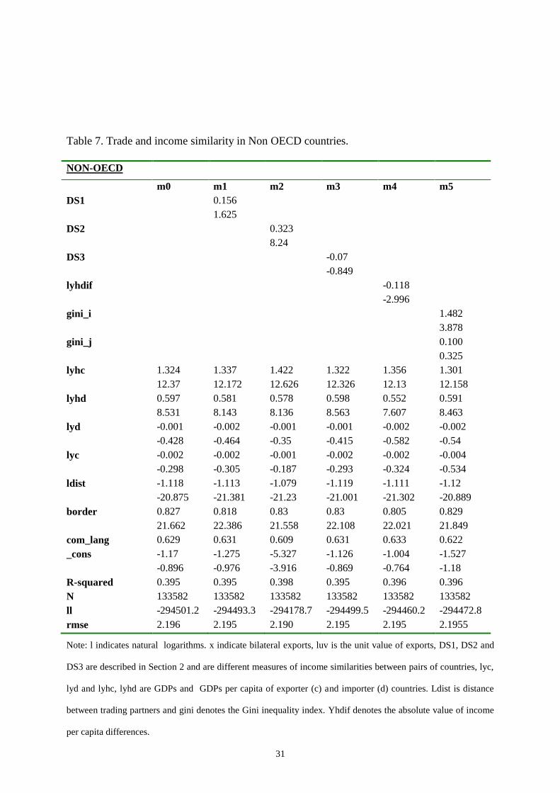
Finally, we estimated similar equations for the rest of countries, obtaining different
results for the income per capita variables that are now also significant for the exporter
country and smaller in magnitude but also significant for the destination market. Table 7
shows the results of estimating equation 2. The main differences with respect to HOECD
countries are that now higher income per capita differences are significantly associated with
lower bilateral trade, whereas higher levels of inequality are associated with higher volumes
of bilateral exports (hypothesis 2).
4. Robustness
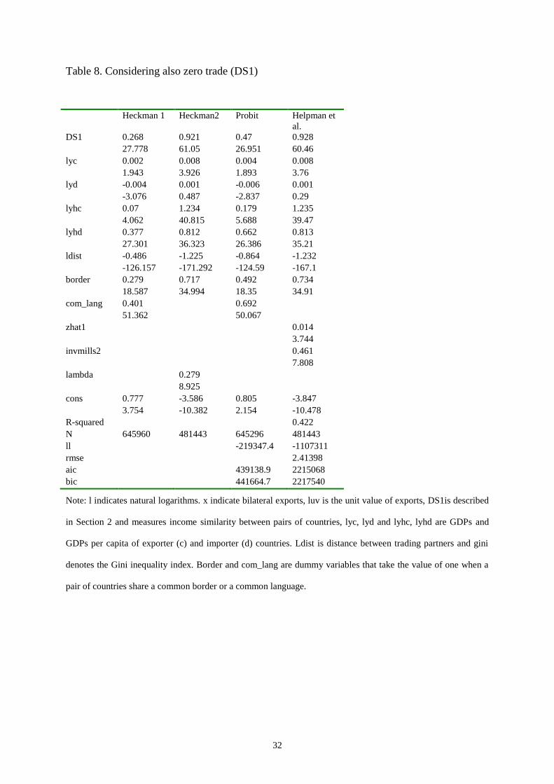
In order to test for the robustness of our results, several additional estimations are
considered. First, we take the zero flow observations into account. Results from four different
estimation techniques are presented in Tables 8 and 9. Columns 1 and 2 (Tables 8 and 9)
report the first and second step results from estimated a Heckman selection model. Columns 3
and 4 (Tables 8 and 9) report the first and second step results from estimated a Helpman et al.
(2008) model. We find significant and positive selection bias5, which is in accordance with
previous research (e.g. Helpman et al, 2008; Hallak, 2006). In addition the estimates that
account for firm heterogeneity (zhat1 and zhat2) are also positive and statistically significant,
indicating that there is also a positive bias steaming from the differences in productivity
across firms. The main results concerning the effect of income distribution similarities on
5 The test for selection bias is the t-statistic of the inverse Mills ratio in the first step (behavioral) equation, which
is highly significant and positively signed.

18
trade remain almost unchanged with respect to the log-linear model (Table 2). For example,
results in Table 9 using the log of DS2 indicate that the effect of a 10 % increase in income-
distribution similarities increases exports by 3.9 % according to the log-linear model
(excluding zero trade) and by 4% according to the Heckman and Helpman et al. models and
by 3.6% according to the gamma specification. The results concerning DS1 (Table 8) and
DS2 are also very similar. With respect to the behavioural equation (step 1), most variables
that impact the amount exported also affect the probability that country i exports to country j
(the country level extensive margin). Specifically, increases in DS1, DS2 and income per
capita increase the probability of exporting. Since in terms of root mean squared error and
according to both information criteria, the results obtained with DS2 are better, we use only
this index for the two following robustness checks.
Second, we estimated a dynamic model adding lagged exports as an additional regressor
and estimating the equation using Arellano and Bond difference GMM estimator. The results
for all countries are shown in Table 10. Once more, with respect to the variables of interest
DS2, the long-run estimated coefficient is 0.23 (=0.137/(1-0.368-0.05)) that is in line with
previous results.
Finally, we try also with different sets of fixed effects. We add dyadic fixed effects in
addition to year and sectoral effects. The results are shown in Table 11.
5. Conclusions
In this paper we present empirical evidence supporting the hypothesis of non-homothetic
preferences stated by Markusen (2010). We also propose three alternative measures of
income distribution similarity between countries. These measures are used to proxy for
demand similarities between pairs of countries across trading partners and over time. Trade
theory in conjunction with some stylized empirical facts indicates that preferences are non-
homothetic; not only the average income but also the distribution of income should influence

19
aggregate demand. Ideally, the full distribution of income should be considered when demand
similarities between countries are measured.
Using the three distribution-based measures as a proxy for demand similarities in gravity
models, we find consistent and robust support for the hypothesis stating that countries with
more similar income-distributions trade more with each other. The hypothesis is also
confirmed at disaggregated level, both for homogenous and for differentiated product
categories. The larger the overlap in income distribution between two countries the higher
will be the extent of trade between the two. In line with the theoretical predictions we also
find that income per capita has a stronger effect for more sophisticated goods in comparison
with more homogenous ones.

20
References
Arad, R. W. & Hirsch, S. (1981) Determination of trade flows and choice of trade partners:
Reconciling the Heckscher-Ohlin and the Burenstam Linder Models of international
trade. Weltwirtschaftliches Archiv, 117, 276-97.
Arnon, A. & Weinblatt, J. (1998) Linder’s hypothesis revisited: income similarity effects for
low income countries. Applied Economic Letters, 5, 607-611.
Baier, S. L. and Bergstrand, J. H. (2007) “Do Free Trade Agreements Actually Increase
Members´ International Trade” Journal of International Economics 71, 72-95.
Baldwin, R. and Taglioni, D. (2006) Gravity for Dummies and Dummies for Gravity
Equations, National Bureau of Economic Research Working Paper 12516, Cambridge.
Bertola, G., Foellmi, R. & Zweimüller, J. (2006) Income distribution in macroeconomic
models Princeton, N.J., Princeton University Press.
Bohman, H. and Nilsson, D. (2007) Market Overlap and the Direction of Exports –A New
Approach of Assesing the LinderHypothesis.CESIS Working Paper, Jonjopkins,
Sweden.
CEPII (2009) dist_cepii.dta. Centre d'Ètudes Prospectives et d'Information Internationales.
Choi, C. (2002) Linder Hypotesis Revisited. Applied Economics Letters, 9, 9, 601-605.
Chul Choi, Y., Hummels, D. & Xiang, C. (2009) Explaining Import Variety and Quality: The
Role of the Income Distribution. Journal of International Economics,77 (2), 265-275.
COMTRADE (2009) United Nations Commodity Trade Statistics Database Statistics division,
United Nations.
Dalgin, M.& Mitra, D. & Trindade, V. (2008) Inequality, Nonhomothetic Preferences, and
Trade: A Gravity Approach. Southern Economic Journal, 74, 3, 747-774.
Fajgelbaum, Pablo D., Grossman, Gene M. and Helpman Elhanan, (2009) Income Distribution,
Product Quality, and International Trade, NBER Working Papers 15329, National Bureau
of Economic Research, Inc.
Falvey, R. & Kierzkowski, H. (1987) Product Quality, Intra-industry Trade and (Im)perfect
Competition". In Kierzkowski, H. (Ed.) Protection and Competition in International
Trade: Essays in Honour of Max Corden. Oxford, Basil Blackwell.
Fieler, A. C. (2009) Non-Homotheticity and Bilateral Trade: Evidence and a Quantitative
Explanation, New York University. Mimeo.
Flam, H. & Helpman, E. (1987) Vertical Product Differentiation and North-South Trade. The
American Economic Review, 77, 810-822.

21
Francois, J. F. & Kaplan, S. (1996) Aggregate demand shifts, income distribution, and the
Linder hypothesis. The Review of Economics and Statistics, 78, 244.
Gruen, C. and Klasen, S. (2008) Growth, inequality and welfare: Comparisons across time
and space. Oxford Economic Papers 60, 212-236.
Hallak, J. C. (2006) Product quality and the direction of trade. Journal of International
Economics, 68, 238-265.
Hallak, J. C. (2010) A product quality view of the Linder hypothesis. The Review of
Economics and Statistics, forthcoming.
Helpman, E. & Melitz, M. & Rubinstein, Y. (2008) Estimating Trade Flows: Trading Partners and Trading Volumes, The Quarterly Journal of Economics, MIT Press, vol. 123(2), pages 441-487, 05.
Heston, A., Summers, R., and Aten, B. (2002) Penn world table version 6.1, Center for
International Comparisons at the University of Pennsylvania (CICUP),
http://pwt.econ.upenn.edu/.
Holzmann, H, Vollmer, S. and Weisbrod, J. (2007) Twin Peaks or Three Components? –
Analyzing the World’s Cross-Country Distribution of Income. IAI Working Papers
158, University of Goettingen, Goettingen, Germany.
Hunter, L. (1991) The Contribution of Nonhomothetic Preferences to Trade. Journal of
International Economics, 30, 345-358.
Hunter, L. & Markusen, J.R. & Rutherford, T.F. (1991) Trade Liberalization in a Multinational-
Dominated Industry: A Theoretical and Applied General-Equilibrium Analysis, NBER
Working Papers 3679, National Bureau of Economic Research.
Linder Burenstam, S. (1961) An Essay on Trade and Transformation Department of
Economics. Stockholm, Stockholm School of Economics.
Markusen, J. (2010) Putting Per-Capita Income back into Trade Theory University of
Colorado, Boulder, Mimeo. http://spot.colorado.edu/~markusen/
Martínez-Zarzoso, I. & Nowak-Lehmann D. (2004) Economic and Geographical Distance:
Explaining Mercosur Exports to the EU. Open Economies Review 15, 3, 291-314.
Matsuyama, K. (2000) A Ricardian model with a continuum of goods under nonhomothetic
preferences: Demand complementarities, income distribution, and North-South trade.
The Journal of Political Economy, 108, 1093.
Mcpherson, M. A., Redfearn, M. R. & Tieslau, M. A. (2000) A re-examination of the Linder
Hypothesis: A random-effects Tobit approach. International Economic Journal, 14,
123-136.
Mcpherson, M. A., Redfearn, M. R. & Tieslau, M. A. (2001) International trade and
developing countries: an empirical investigation of the Linder hypothesis. Applied
Economics, 33, 649-657.

22
Mitra, D. & Trindade, V. (2005) Inequality and trade. The Canadian Journal of Economics,
38, 1253.
Rauch, J. E. (1999) Networks Versus Markets in International Trade. Journal of International
Economics, 48, 7-35.

23
Figure 1 Illustration of Overlaps for China and the U.S., 1970
Left figure: Density of GDP p.c. for China (dashed line) and the U.S. (solid line). Right figure: Density of GDP
p.c. For China (dashed line) and the U.S. (solid line) multiplied by population size.
Figure 2 Illustration of Overlaps for China and the U.S., 2003
Left figure: Density of GDP p.c. for China (dashed line) and the U.S. (solid line). Right figure: Density of GDP
p.c. For China (dashed line) and the U.S. (solid line) multiplied bypopulation size.
Table 1 Development of the different measures over time (example China and the
U.S.)
DS 1 and 3 are index values (range 0 to 1). DS 2 is measured in thousands of people.
Year DS1 DS2 DS3 CHN DS3 USA
1970 .002 825 .001 .004
1975 .004 1462 .002 .007
1980 .008 3574 .004 .015
1985 .023 9599 .009 .039
1990 .054 26079 .023 .102
1995 .114 58117 .048 .216
2000 .165 88347 .070 .311
2003 .221 128216 .100 .438

24
Table 2. Summary statistics
Variable Obs Mean Std. Dev. Min Max
lx 481766 5.852 3.176 -0.691 18.014
lxuv 450810 5.340 1.990 20.504 11.775
DS1 645960 0.448 0.292 0.000 0.998
DS2 645960 8.310 1.373 1.569 17.963
DS3 645960 0.403 0.359 0.000 1.000
lyc 645960 30.121 3.026 20.405 36.394
lyd 645960 30.107 2.983 20.405 36.394
lyhc 645960 9.014 1.035 6.186 10.460
lyhd 645960 8.806 1.110 5.884 10.460
ldist 645960 8.675 0.838 1.792 9.899
lgini 645960 -1.692 0.303 -2.768 -0.510
gini_i 645960 0.433 0.091 0.238 0.792
gini_j 645960 0.444 0.097 0.238 0.792
Note: l indicates natural logarithms. x indicate bilateral exports, luv is the unit value of exports, DS1, DS2 and
DS3 are described in Section 2 and are different measures of income similarities between pairs of countries, lyc,
lyd and lyhc, lyhd are GDPs and GDPs per capita of exporter (c) and importer (d) countries. Ldist is distance
between trading partners and gini denotes the Gini inequality index.

25
Table 3. Income similarity and exports (Equation 2)
Baseline Index 1 DS2 DS3 yh diff gini coeff
m0 m1 m2 m3 m4 m5
DS1 0.855
12.747
DS2 0.41
17.317
DS3 0.644
11.041
lyhdif -0.363
-13.241
gini_i 0.229
1.133
gini_j 0.495
3.094
lyhc 1.272 1.253 1.279 1.282 1.269 1.268
11.465 11.106 11.17 11.392 11.068 11.385
lyhd 0.955 0.874 0.818 0.884 0.786 0.952
21.712 19.942 18.238 20.52 17.37 21.53
lyc 0.01 0.01 0.009 0.01 0.008 0.01
2.976 2.897 2.876 3.00 2.523 3.045
lyd 0.003 0.002 0000 0.001 0.001 0.002
1.447 1.144 0.135 0.627 0.592 1.34
ldist -1.303 -1.235 -1.212 -1.265 -1.225 -1.304
-32.532 -32.192 -32.467 -31.846 -32.451 -32.605
border 0.829 0.699 0.691 0.764 0.665 0.83
20.75 17.636 17.198 19.934 16.539 20.689
com_lang 0.869 0.828 0.873 0.85 0.846 0.867
12.909 12.728 13.031 12.85 12.886 12.837
R2 0.54 0.544 0.547 0.542 0.546 0.54
N 481766 481766 481766 481766 481766 481766
ll 1053004 1050938 1049194 1052170 1049955 1052987
rmse 2.153 2.144 2.136 2.149 2.139 2.153
aic 2106061 2101930 2098442 2104394 2099965 2106028
bic 2106361 2102229 2098741 2104693 2100264 2106328
Country and
Time Dummies
Yes Yes Yes Yes Yes Yes
ISIC 3D
dummies
Yes Yes Yes Yes Yes Yes
Note: l indicates natural logarithms..DS1, DS2 and DS3 are described in Section 2 and are different measures of
income similarities between pairs of countries, lyc, lyd and lyhc, lyhd are GDPs and GDPs per capita of
exporter (c) and importer (d) countries. Ldist is distance between trading partners and gini denotes the Gini
inequality index. Border and com_lang are dummy variables that take the value of one when a pair of countries

26
share a common border or a common language. Yhdif denotes the absolute value of income per capita
differences.
Table 4. Sectoral results (INDEX 1)
Food Products Beverages
&Tobacco
Textiles
and
Footwear
Wood,
paper
Chemicals,
Rubber,
Plastic
Pottery,
Glass,
ceramic
products
Iron,
steel.
Other
metals
Transport
equipment
Machinery
and other
manufactures
Food
Products
m311 m313 m32 m33 m35 m36 m371 m384 m38
DS1 0.635 0.703 0.623 0.791 0.995 1.016 0.719 1.164 1.18
8.265 6.233 10.646 13.452 18.024 16.863 8.932 14.23 26.056
gini_i -0.168 -1.15 0.333 -0.142 0.371 0.318 -0.284 -0.901 0.011
-0.372 -1.975 1.038 -0.417 1.259 0.764 -0.588 -1.584 0.046
gini_j 1.591 0.945 1.442 0.329 0.544 0.187 -0.232 1.351 0.341
3.799 1.901 5.38 1.188 2.347 0.657 -0.573 3.031 1.673
lyc 0.007 0.000 0.016 0.017 0.007 0.02 -0.002 0.001 -0.003
1.11 -0.013 4.034 3.991 1.712 4.037 -0.335 0.123 -0.959
lyd -0.004 0.017 0.001 -0.001 0.006 -0.006 0.009 0.002 -0.002
-0.681 2.264 0.228 -0.406 2.038 -1.372 1.454 0.268 -0.836
lyhc 0.596 0.52 1.11 1.122 1.5 1.119 0.969 2.109 1.762
5.256 3.397 14.883 14.791 22.921 12.499 8.778 15.442 31.253
lyhd 0.762 0.592 0.941 0.978 0.632 0.827 1.018 0.986 1.056
8.559 5.578 15.763 16.288 13.099 13.235 12.296 9.633 23.71
ldist -1.287 -1.072 -1.091 -1.349 -1.223 -1.305 -1.478 -1.259 -1.286
-39.002 -27.38 -45.837 -58.407 -53.649 -54.271 -48.415 -33.957 -65.928
border 0.817 0.708 0.761 0.589 0.595 0.778 0.241 0.929 0.568
5.939 4.787 8.921 7.074 7.093 8.216 2.155 6.645 7.377
com_lang 0.823 0.536 0.792 0.966 0.627 0.742 0.683 0.98 1.111
11.652 5.927 15.165 18.443 12.74 13.69 9.3 12.967 27.098
cons 6.133 1.668 -6.169 -4.664 -4.763 -4.228 0.73 -12.31 -10.081
4.649 0.985 -6.633 -5.146 -6.18 -4.165 0.571 -7.786 -14.581
R-squared 0.603 0.446 0.49 0.524 0.448 0.548 0.551 0.677 0.679
N 23435 20108 69078 66683 97443 44734 31454 20158 88241
ll -47785.36 -44020.52 -152578.6 -144029.4 -219316.9 -91381.14 -67694.78 -41935.77 -181229.7
rmse 1.868 2.172 2.206 2.1015 2.3001 1.871 2.089 1.948 1.889
aic 96020.72 88487.03 305605.1 288508.8 439083.9 183204.3 135839.6 84319.54 362909.4
bic 97834.67 90250.71 307653.2 290558 441218.5 185128.9 137719.7 86091.69 365021.6
Time
dummies
Yes Yes Yes Yes Yes Yes Yes Yes Yes
X, M
dummies
Yes Yes Yes Yes Yes Yes Yes Yes Yes
Sectoral
dummies
Yes Yes Yes Yes Yes Yes Yes Yes Yes
Note: l indicates natural logarithms. x indicate bilateral exports, luv is the unit value of exports, DS1 is described
in Section 2 and measures income similarities between pairs of countries, lyc, lyd and lyhc, lyhd are GDPs and
GDPs per capita of exporter (c) and importer (d) countries. Ldist is distance between trading partners and gini
denotes the Gini inequality index. The ISIC trade classification has been used. Border and com_lang are dummy
variables that take the value of one when a pair of countries shares a common border or a common language.

27
Table 5. Export unit values and income variables
Food
Products
Beverages&
Tobacco
Textiles and
Footwear
Wood,
paper
Chemicals,
Rubber,
Plastic
Pottery,
Glass ,
ceramic
Iron, steel.
Other
metals
Transport
equipment
Machinery
and other
manufactures
All Sectors m311 m313 m32 m33 m35 m36 m371 m384 m38
DS1 -0.11 0.14 0.14 0.07 -0.10 -0.10 -0.15 -0.21 0.10 -0.28
-2.67 4.06 2.08 2.45 -2.42 -2.48 -3.14 -4.08 1.55 -6.89
gini_i 1.23 0.00 2.43 1.98 0.47 0.73 1.09 0.18 0.87 1.58
4.66 0.00 4.08 9.85 1.92 3.32 3.47 0.69 1.37 6.44
gini_j -0.25 -0.35 -0.52 0.20 -0.13 -0.27 -0.23 -0.58 -0.06 -0.39
-3.62 -1.81 -0.98 1.38 -0.71 -1.76 -1.02 -2.41 -0.15 -2.25
lyc 0.01 0.01 0.02 0.00 0.01 0.01 0.03 0.01 0.02 0.02
3.52 1.92 1.99 1.13 1.85 3.56 6.10 1.05 1.59 4.93
lyd 0.00 0.00 0.00 0.00 0.00 0.00 0.00 0.00 0.00 0.00
0.46 0.76 -0.19 -0.50 1.49 0.29 1.10 0.27 -0.34 -0.34
lyhc -0.13 0.14 0.56 -0.19 0.05 -0.09 0.09 0.11 -0.47 -0.58
-1.34 2.52 3.45 -4.52 0.94 -1.90 1.14 1.67 -3.15 -9.91
lyhd 0.00 0.01 0.06 0.16 -0.07 -0.04 0.07 -0.05 0.06 -0.10
0.13 0.14 0.49 4.93 -1.62 -1.26 1.33 -1.02 0.57 -2.38
ldist 0.23 0.21 0.18 0.05 0.23 0.33 0.44 0.29 0.22 0.25
9.85 15.85 7.98 4.82 13.74 22.17 20.87 14.94 8.33 15.16
border -0.15 -0.14 -0.30 -0.12 -0.13 -0.15 -0.18 0.01 -0.05 -0.14
-5.69 -2.77 -3.59 -3.03 -2.31 -2.94 -2.46 0.18 -0.54 -2.47
com_lang -0.03 0.05 -0.04 0.01 0.01 0.01 -0.02 0.05 -0.05 -0.19
-1.05 1.70 -0.72 0.23 0.17 0.23 -0.34 1.12 -0.87 -5.33
cons -8.57 -10.71 -16.33 -5.70 -8.32 -8.21 -13.55 -9.69 -4.37 -1.04
-9.03 -17.20 -8.78 -11.19 -13.13 -15.47 -15.26 -13.36 -2.57 -1.54
R2 0.40 0.29 0.21 0.32 0.14 0.14 0.27 0.19 0.52 0.25
N 450810 22691 19306 65161 61353 92020 40969 30443 18891 82193
ll -835692.00 -30878.75 -38506 -104472 -110765 -174557.4 -76190.3 -51226.6 -38992.1 -162657.7
rmse 1.55 0.95 1.79 1.20 1.47 1.61 1.56 1.31 1.92 1.75
aic 1671438.00 62205.49 77456.77 209390.60 221977.90 349562.80 152820.70 102901.40 78428.17 325763.40
bic 1671735.00 64004.15 79203.50 211416.50 223999.40 351675.10 154717.30 104765.80 80170.08 327850.40
Time Yes Yes Yes Yes Yes Yes Yes Yes Yes Yes

28
dummies
X,M
dummies
Yes Yes Yes Yes Yes Yes Yes Yes Yes Yes
Note: l indicates natural logarithms. x indicate bilateral exports, luv is the unit value of exports, DS1is described in Section 2 and measures income similarities between pairs of
countries, lyc, lyd and lyhc, lyhd are GDPs and GDPs per capita of exporter (c) and importer (d) countries. Ldist is distance between trading partners and gini denotes the Gini
inequality index. The ISIC trade classification has been used.

29
Table 6. Trade and income similarity in OECD countries. Estimation of equations 2 and 3
HOECD HOECD with X-t and M-t dummies
m0 m1 m2 m3 m4 m5 m1 m2 m3 m4 m5
DS1 0.191 DS1 0.149
1.535 1.374
DS2 0.274 lDS2 0.275
8.627 8.437
DS3 0.332 DS3 0.341
5.597 5.604
lyhdif -0.072 yhdif -0.038
-1.022 -0.446
gini_i -1.99 ginidif 1.241
-4.168 3.841
gini_j 1.378
4.634
lyhc 0.037 -0.006 0.001 0 0.012 0.066
0.186 -0.027 0.007 0 0.06 0.33
lyhd 1.435 1.39 1.394 1.408 1.409 1.412
17.53 15.097 16.884 17.119 15.909 17.132
R-squared 0.703 0.703 0.704 0.703 0.703 0.703 R-squared 0.708 0.709 0.708 0.708 0.708
N 54245 54245 54245 54245 54245 54245 N 54245 54245 54245 54245 54245
ll -103359.5 -103357.4 -103245.1 -103338.3 -103358.6 -103331.5 ll -102824.6 -102708.5 -102803.1 -102825.5 -102816.1
ISIC 3D dummies Yes Yes Yes Yes Yes Yes Yes Yes Yes Yes Yes
Country and year
Dummies
Yes Yes Yes Yes Yes Yes

30
Note: l indicates natural logarithms. x indicate bilateral exports, luv is the unit value of exports, DS1, DS2 and DS3 are described in Section 2 and are different measures of
income similarities between pairs of countries, lyc, lyd and lyhc, lyhd are GDPs and GDPs per capita of exporter (c) and importer (d) countries. Ldist is distance between trading
partners and gini denotes the Gini inequality index. Yhdif denotes the absolute value of income per capita differences.
31
Table 7. Trade and income similarity in Non OECD countries.
NON-OECD
m0 m1 m2 m3 m4 m5
DS1 0.156
1.625
DS2 0.323
8.24
DS3 -0.07
-0.849
lyhdif -0.118
-2.996
gini_i 1.482
3.878
gini_j 0.100
0.325
lyhc 1.324 1.337 1.422 1.322 1.356 1.301
12.37 12.172 12.626 12.326 12.13 12.158
lyhd 0.597 0.581 0.578 0.598 0.552 0.591
8.531 8.143 8.136 8.563 7.607 8.463
lyd -0.001 -0.002 -0.001 -0.001 -0.002 -0.002
-0.428 -0.464 -0.35 -0.415 -0.582 -0.54
lyc -0.002 -0.002 -0.001 -0.002 -0.002 -0.004
-0.298 -0.305 -0.187 -0.293 -0.324 -0.534
ldist -1.118 -1.113 -1.079 -1.119 -1.111 -1.12
-20.875 -21.381 -21.23 -21.001 -21.302 -20.889
border 0.827 0.818 0.83 0.83 0.805 0.829
21.662 22.386 21.558 22.108 22.021 21.849
com_lang 0.629 0.631 0.609 0.631 0.633 0.622
_cons -1.17 -1.275 -5.327 -1.126 -1.004 -1.527
-0.896 -0.976 -3.916 -0.869 -0.764 -1.18
R-squared 0.395 0.395 0.398 0.395 0.396 0.396
N 133582 133582 133582 133582 133582 133582
ll -294501.2 -294493.3 -294178.7 -294499.5 -294460.2 -294472.8
rmse 2.196 2.195 2.190 2.195 2.195 2.1955
Note: l indicates natural logarithms. x indicate bilateral exports, luv is the unit value of exports, DS1, DS2 and
DS3 are described in Section 2 and are different measures of income similarities between pairs of countries, lyc,
lyd and lyhc, lyhd are GDPs and GDPs per capita of exporter (c) and importer (d) countries. Ldist is distance
between trading partners and gini denotes the Gini inequality index. Yhdif denotes the absolute value of income
per capita differences.
32
Table 8. Considering also zero trade (DS1)
Heckman 1 Heckman2 Probit Helpman et
al.
DS1 0.268 0.921 0.47 0.928
27.778 61.05 26.951 60.46
lyc 0.002 0.008 0.004 0.008
1.943 3.926 1.893 3.76
lyd -0.004 0.001 -0.006 0.001
-3.076 0.487 -2.837 0.29
lyhc 0.07 1.234 0.179 1.235
4.062 40.815 5.688 39.47
lyhd 0.377 0.812 0.662 0.813
27.301 36.323 26.386 35.21
ldist -0.486 -1.225 -0.864 -1.232
-126.157 -171.292 -124.59 -167.1
border 0.279 0.717 0.492 0.734
18.587 34.994 18.35 34.91
com_lang 0.401 0.692
51.362 50.067
zhat1 0.014
3.744
invmills2 0.461
7.808
lambda 0.279
8.925
cons 0.777 -3.586 0.805 -3.847
3.754 -10.382 2.154 -10.478
R-squared 0.422
N 645960 481443 645296 481443
ll -219347.4 -1107311
rmse 2.41398
aic 439138.9 2215068
bic 441664.7 2217540
Note: l indicates natural logarithms. x indicate bilateral exports, luv is the unit value of exports, DS1is described
in Section 2 and measures income similarity between pairs of countries, lyc, lyd and lyhc, lyhd are GDPs and
GDPs per capita of exporter (c) and importer (d) countries. Ldist is distance between trading partners and gini
denotes the Gini inequality index. Border and com_lang are dummy variables that take the value of one when a
pair of countries share a common border or a common language.

33
Table 9. Considering also zero trade (DS2)
exp_tv lx exp_tv lx exp_tv exp_tv
Heckman 1 Heckman2 Probit Helpman et
al.
Poisson Gamma
DS2 0.16 0.405 0.099 0.407 0.079 0.362
26.797 74.974 31.476 74.088 2.299 29.407
lyc 0.004 0.008 0.002 0.008 0.015 0.011
1.891 3.846 1.972 3.689 1.653 1.886
lyd -0.007 -0.001 -0.004 -0.001 0.005 0.007
-3.016 -0.477 -3.306 -0.672 0.745 1.721
lyhc 0.197 1.258 0.08 1.259 1.246 1.333
6.268 41.652 4.653 40.388 9.058 17.39
lyhd 0.669 0.777 0.378 0.778 0.979 0.64
26.656 34.755 27.41 33.766 8.631 13.001
ldist -0.855 -1.232 -0.48 -1.239 -0.677 -1.031
-122.341 -174.022 -123.791 -169.226 -47.441 -80.667
border 0.503 0.736 0.281 0.752 1.143 0.743
18.821 36.057 18.808 36.001 20.643 19.883
com_lang 0.714 0.414 -0.04 0.675
51.768 53.155 -0.808 24.971
zhat2 0.013
3.399
invmills 0.413 0.58
13.248 9.776
cons -0.738 -6.771 -0.176 -7.016 -8.373 -5.317
-1.944 -19.451 -0.838 -18.963 -5.692 -6.596
R-squared 0.424
N 645296 481443 645960 481443 645960 645960
ll -219326 -1106366 -1.73E+10 -5431013
rmse 2.409249
aic 439096 2213179 3.46E+10 1.68E+01
bic 441621.8 2215651 3.46E+10 -6.23E+06
Note: l indicates natural logarithms. x indicate bilateral exports, luv is the unit value of exports, DS2 is described
in Section 2 and measures income similarity between pairs of countries, lyc, lyd and lyhc, lyhd are GDPs and
GDPs per capita of exporter (c) and importer (d) countries. Ldist is distance between trading partners and gini
denotes the Gini inequality index. Border and com_lang are dummy variables that take the value of one when a
pair of countries share a common border or a common language.

34
Table 10: Difference GMM
m1
b/t
lx(-1) 0.368
49.386
lx(-2) 0.05
13.402
DS2 0.137
3.504
gini_i 0.412
2.007
gini_j 0.76
5.209
lyc -0.002
-1.209
lyd 0.003
1.917
lyhc -0.082
-1.984
lyhd 1.344
30.49
t4 0.027
2.724
t5 -0.282
-18.996
t6 -0.245
-14.772
cons -8.361
Ar(1) p 0.00
Ar(2) p 0.10
N 223244
Note: l indicates natural logarithms. x indicate bilateral exports, luv is the unit value of exports, DS2 is described
in Section 2 and measures income similarity between pairs of countries, lyc, lyd and lyhc, lyhd are GDPs and
GDPs per capita of exporter (c) and importer (d) countries. Gini denotes the Gini inequality index.

35
Table 11. With exporter-importer-sectoral and time fixed effects
fe0 fe2 fe4 fe5
b/t b/t b/t b/t
DS2 0.211
13.224
gini_i -0.944 -0.618
-8.344 -5.633
gini_j 1.039 1.21
11.972 14.03
lyhdif -0.224
-10.284
lyhc 1.439 1.461 1.442 1.454
53.457 53.567 53.595 53.207
lyhd 1.495 1.367 1.329 1.486
77.284 63.677 51.839 76.831
lyc 0.013 0.011 0.012 0.012
8.717 7.855 8.419 8.053
lyd 0.004 0.003 0.004 0.004
3.222 2.05 2.907 3.052
t2 -0.226 -0.229 -0.211 -0.228
-26.484 -26.549 -24.436 -26.373
t3 0.18 0.167 0.219 0.171
16.701 15.479 19.266 15.851
t4 0.515 0.493 0.569 0.504
40.561 38.69 41.653 39.553
t5 0.318 0.3 0.395 0.307
20.054 18.964 22.694 19.377
t6 0.404 0.383 0.485 0.394
23.766 22.576 26.089 23.174
cons -21.3 -22.145 -19.623 -21.603
-73.227 -75.235 -58.886 -74.088
R-squared 0.214 0.216 0.215 0.215
N 481766 481766 481766 481766
ll -759940.4 -759487.3 -759785.8 -759697.8
rmse 1.1717 1.1706 1.1713 1.1711
Note: l indicates natural logarithms. DS2 is described in Section 2 and measures income similarities between
pairs of countries, lyc, lyd and lyhc, lyhd are GDPs and GDPs per capita of exporter (c) and importer (d)
countries. Ldist is distance between trading partners and gini denotes the Gini inequality index. Yhdif denotes
the absolute value of income per capita differences.