Journal of Public Economics 76 (2000) 459–493www.elsevier.nl / locate /econbase

Dodging the grabbing hand: the determinants ofunofficial activity in 69 countries

a b , c*Eric Friedman , Simon Johnson , Daniel Kaufmann ,cPablo Zoido-Lobaton

aRutgers, New Brunswick, NJ 08903, USAbSloan School of Management, MIT, Cambridge, MA, 02142, USA

cThe World Bank, Washington, DC, USA

Abstract

Across 69 countries, higher tax rates are associated with less unofficial activity as apercent of GDP but corruption is associated with more unofficial activity. Entrepreneurs gounderground not to avoid official taxes but to reduce the burden of bureaucracy andcorruption. Dodging the ‘grabbing hand’ in this way reduces tax revenues as a percent ofboth official and total GDP. As a result, corrupt governments become small governmentsand only relatively uncorrupt governments can sustain high tax rates. 2000 ElsevierScience S.A. All rights reserved.

Keywords: Corruption; Over-regulation; Taxation; Legal system; Unofficial economy

JEL classification: H26; K42; O17

1. Introduction

What drives entrepreneurs and large businesses underground? One school ofthought identifies high tax rates as the main culprit. In other words, companies thatoperate in the unofficial economy are simply trying to keep all of their profits forthemselves. An alternative view holds that when unregistered economic activityrises, the political and social institutions that govern the economy are to blame.

*Corresponding author. Tel.: 11-617-253-8412; fax: 11-617-253-2660.E-mail address: sjohnson@mit.edu (S. Johnson)

0047-2727/00/$ – see front matter 2000 Elsevier Science S.A. All rights reserved.PI I : S0047-2727( 99 )00093-6

460 E. Friedman et al. / Journal of Public Economics 76 (2000) 459 –493

According to this theory, bureaucracy, corruption, and a weak legal system bearprimary responsibility for driving businesses underground. Firm managers may bewilling to be taxed at a reasonable rate, but they are unwilling to put up withconstant extortionate and arbitrary demands.

A Western manager who decided against locating a plant in Russia illustrates thelogic behind the second view. He explains: ‘It doesn’t matter who it is: fireinspector, zoning committee member, mayor for that region, anybody can comeand shut you down in 5 min. The fire guy could come, find fire hazards, anddemand $50,000 into his overseas account. They know that if you shut downproduction for a few days, you’re going to lose a lot more’ (Wilson, 1996). Facedwith this hostile environment, foreign firms may choose to locate elsewhere.However, for local entrepreneurs seeking to avoid the same risks, the usual courseis to go underground (Kaufmann, 1997).

This paper evaluates these two theories using 1990s data for tax rates,bureaucracy, corruption, the legal environment, and the size of the unofficial

1economy in 69 countries. Our analysis reveals no evidence that higher direct orindirect tax rates are associated with a larger unofficial economy. In fact, we findsome evidence that higher direct tax rates are associated with a smaller under-ground sector. However, when we control for per capita income, in order to allowfor the possibility that richer countries have better-run administrations and highertax rates, the relationship ceases to be significant. By contrast, more bureaucracy,greater corruption, and a weaker legal environment are all associated with a largerunofficial economy, even (in most cases) when we control for per capita income.

This result suggests that poor institutions and a large unofficial economy gohand in hand. It does not, however, resolve the question of which comes first: dopoor institutions cause high levels of underground activity, or do high levels ofunderground activity undermine basic institutions? To address this issue, we use aset of exogenous instrumental variables, developed by La Porta et al. (1999), thatmeasure long-standing linguistic fractionalization, the origins of the legal system,the religious composition of the population, and geographic location (latitude). LaPorta et al. (1999) show that these variables are significantly correlated withinstitutional development across a wide range of countries. The instrumentalvariable results in our regressions show there is an exogenous component of‘institutions’ that is significantly correlated with the size of the unofficialeconomy. This suggests a causal link running from weak economic institutions toa large unofficial economy.

A simple story can explain this result: when faced with onerous bureaucracy,high levels of corruption, and a weak legal system, businesses hide their activities

1Other than for a few OECD countries, there is no time series data on the unofficial economy for anysignificant time period (Schneider and Enste, 1998).

E. Friedman et al. / Journal of Public Economics 76 (2000) 459 –493 461

2‘underground’. Consequently, tax revenues fall, and the quality of publicadministration declines accordingly, further reducing a firm’s incentives to remain‘official’. Supporting evidence for this story is found in the fact that poorinstitutions are also associated with lower tax revenue as a share of GDP.

This paper builds on earlier work, in which we focus on establishing a linkbetween institutions and the unofficial economy in the formerly communistcountries of Eastern Europe and the FSU, in the OECD, and in Latin America(Johnson et al., 1997, 1998). In this paper we test these findings against thealternative hypothesis that tax rates largely determine the size of the unofficialeconomy. We also build on the growing literature that examines the implications ofinstitutions for output, growth, and government revenue (Delong and Shleifer,1993; Knack and Keefer, 1995; Mauro, 1995; Easterly and Levine, 1997; Shleifer,1997; La Porta et al., 1999). Previous work in this area has shown that poorinstitutions are correlated with lower government revenue both in absolute termsand as a percent of GDP (La Porta et al., 1999). Our findings help explain howpoor institutions undermine the tax base by inducing more activity to move intothe unofficial economy.

Section 2 explains the theoretical framework and testable predictions. Section 3summarizes the available data. Section 4 presents our main results. Section 5concludes.

2. Diversion into the unofficial economy

Consider the following simple model of an entrepreneur’s decision to operate3officially or unofficially. The entrepreneur can operate fully in the official

economy or divert some resources to the unofficial economy. We model his4decision of how to allocate retained earnings, Y. To the extent he operates

officially, these earnings are invested in a project that earns a gross rate of return

2The most detailed and persuasive description of how bureaucratic red tape and corruption affectsbusiness is De Soto (1989).

3The basic idea is similar to the model of stealing in Johnson et al. (2000), although they deal withthe theft of resources from shareholders by managers and do not deal directly with public financeaspects.

4The key simplifying assumptions are that this is a one period decision problem and the firm doesnot save earnings to invest in the future. There is also no capital market, so the firm cannot borrow orissue equity. We have relaxed these assumptions in a dynamic model with debt, but this morecomplicated analysis does not help with the important public finance issues of this paper (Friedman andJohnson, 1999).

462 E. Friedman et al. / Journal of Public Economics 76 (2000) 459 –493

5R(T ) . 1, where T is tax revenue. The proceeds of operating officially are taxed atrate t. There is also a deadweight over-regulation or bureaucracy cost, at rate r per

6unit of output.If the entrepreneur diverts resources underground, he cannot use them in his

main production process but instead in another lower productivity activity. Let Dbe the amount of resources diverted. To simplify the model we assume that this

7process directly generates value D for the entrepreneur. Furthermore, there is acost of operating underground because the entrepreneur may be caught and

2punished. This cost is denoted kD /2, where k is a parameter that measures theeffectiveness of the legal system. The idea behind this functional form is that it iseasy to divert a small amount of resources but the marginal value of diversion falls

8as the level of diversion increases. For example, the diversion may become easierto observe for the government or courts.

Note that productivity in the official sector, R(T ), depends on the level of taxrevenues. This assumption is designed to capture the important point that if taxrevenues are used wisely they can raise productivity through improved educationor better roads or stronger law and order. In our model, the government has twopositive functions: it provides productivity-enhancing public goods, represented byR(T ), and it maintains a legal system that penalizes firms for diverting resourcesunderground, represented by k. If the legal system is stronger, k is higher and there

9is a higher expected penalty for operating underground.The entrepreneur maximizes utility:

2Max U(D; R, k, t, r) 5 Max[(1 2 t 2 r)(Y 2 D)R(T ) 1 D 2 (kD /2)].D

The optimal amount of diversion, D*, is found by solving:

5We could also assume that this rate of return is higher when k is higher, i.e. law and order isstronger: R9(k) . 0. Assuming that R depends on T is slightly more general, because it allows for thegovernment to produce productivity-enhancing public goods other than law and order, e.g. educationand roads.

6The over-regulation or bureaucracy cost is intended to represent costs imposed on business bybureaucrats from which the government obtains no revenue and which do not generate any positivebenefits for society. Alternatively, we could refer to this term as corruption. It is quite distinct fromregulations that have a positive social impact (e.g. environmental or safety rules).

7Strictly speaking, the entrepreneur should be able to earn a return on money invested in theunofficial activity. However, it simplifies our analysis to assume that the gross return in this activity isjust equal to 1.

8More generally, we just need to assume that the cost of diverting resources is convex. This isnecessary to simplify the analysis.

9Theoretically, k could also be high in a dictatorship that shoots people for operating underground.Empirically this does not appear to be the case. Weaker civil liberties are strongly correlated with moreunofficial activity. At least for the countries in our sample, this is because dictatorships are corrupt andthis corruption affects the legal system also, so prosecutors and judges can be bribed and it is hard toenforce any rules.

E. Friedman et al. / Journal of Public Economics 76 (2000) 459 –493 463

≠U D*] ]S D5 1 2 2 (1 2 t 2 r)R(T ) 5 0,≠D k

which yields,

1]S DD*(R, t, r, k) 5 (1 2 (1 2 t 2 r)R(T )), if D* , Yk

5 Y otherwise.

We assume that (1 2 r)R(T ) , 1, so there is always an incentive to divert a portion10of the retained earnings.

The comparative statics predictions are straightforward for the bureaucracyparameter, r. According to this model, more bureaucracy increases the incentive todivert resources into unofficial activities and thus depresses the overall level ofeconomic activity. In contrast, the relationship between diversion and the tax rate,t, and the quality of the legal environment, k, is more complicated. There is animportant link through the effect of diversion on government revenue and on theability of the government to provide important public services, such as legalenforcement.

Government revenue equals the product of the tax rate and production in theofficial sector,

T 5 tR(T )(Y 2 D*).

We assume that tax revenue is used to produce ‘law and order’:

k 5 k(T ).

Higher taxation increases the incentive to divert resources but it may, dependingon the nature of the initial equilibrium, also increase the level of law and order and

11other productivity-enhancing public goods, which reduces the incentive to divert.Bureaucracy is assumed not to generate any government revenue, so morebureaucracy (i.e. higher r) simply increases the incentive to hide economicactivity.

Consider the simplest case with fixed k and R, K(T ) 5 k and R(T ) 5 R. We setY51 to simplify the notation. Then an equilibrium satisfies D* 5 [1 2 (1 2 t 2

r)R] /k and thus tax revenue is T 5 tR(1 2 D*). Now assume that a 5 [1 2 (1 22(1 2 r)R)]R /k . 0, and define b 5 R /k. The ‘Laffer equation’ that relates tax

revenue to the tax rate is now:

T(t) 5 tR(a 2 tb),

10This assumption simplifies the analysis without affecting the basic intuition.11For an equilibrium model based on the idea that maintaining a legal system is costly and requires

revenue see Johnson et al. (1997). In their model, countries are likely to move to extreme equilibriawith either a high or low level of public goods.

464 E. Friedman et al. / Journal of Public Economics 76 (2000) 459 –493

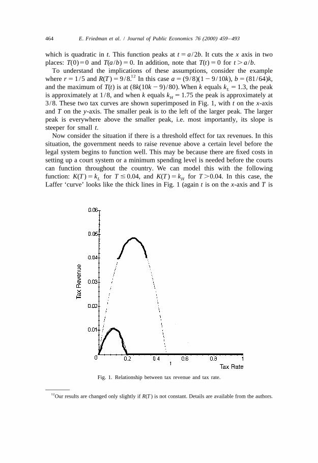
which is quadratic in t. This function peaks at t 5 a /2b. It cuts the x axis in twoplaces: T(0)50 and T(a /b) 5 0. In addition, note that T(t) 5 0 for t . a /b.

To understand the implications of these assumptions, consider the example12where r 5 1/5 and R(T ) 5 9/8. In this case a 5 (9 /8)(1 2 9/10k), b 5 (81 /64)k,

and the maximum of T(t) is at (8k(10k 2 9) /80). When k equals k 5 1.3, the peakL

is approximately at 1 /8, and when k equals k 5 1.75 the peak is approximately atH

3/8. These two tax curves are shown superimposed in Fig. 1, with t on the x-axisand T on the y-axis. The smaller peak is to the left of the larger peak. The largerpeak is everywhere above the smaller peak, i.e. most importantly, its slope issteeper for small t.

Now consider the situation if there is a threshold effect for tax revenues. In thissituation, the government needs to raise revenue above a certain level before thelegal system begins to function well. This may be because there are fixed costs insetting up a court system or a minimum spending level is needed before the courtscan function throughout the country. We can model this with the followingfunction: K(T ) 5 k for T # 0.04, and K(T ) 5 k for T .0.04. In this case, theL H

Laffer ‘curve’ looks like the thick lines in Fig. 1 (again t is on the x-axis and T is

Fig. 1. Relationship between tax revenue and tax rate.

12Our results are changed only slightly if R(T ) is not constant. Details are available from the authors.

E. Friedman et al. / Journal of Public Economics 76 (2000) 459 –493 465

on the y-axis). This relationship is actually a correspondence because it ismulti-valued under the top peak.

The intuition behind this result is that it is always possible to be in equilibriumon the lower curve. In this case, entrepreneurs expect k to be low, so they divertmore to the underground economy, which means that the government raisesrelatively little revenue and can only afford to provide k at a low level. However,there exists another set of equilibria in which entrepreneurs expect k to be high, sothe government is able to raise more revenue and fund a higher level of k.

The model suggests an important contrast between the effects of bureaucraticover-regulation and corruption on the one hand and tax rates on the other hand.More over-regulation and corruption constitute an unambiguous disincentive toproduce in the official sector and should be correlated with a higher share ofunofficial activity. We would expect them also to be correlated with lowergovernment revenue as a percent of GDP and a weaker legal environment.

In contrast, higher tax rates have two potentially offsetting effects: the directeffect increases the incentive to hide activity, but the indirect effect — through theprovision of a better legal environment — encourages production in the officialsector. The model suggests that a higher tax rate will not necessarily be correlatedwith a higher share of unofficial activity. Higher tax rates will also not necessarilybe correlated with government revenue as a percent of GDP or with the strength ofthe legal environment.

3. The data

3.1. Measures of the unofficial economy

Data on the unofficial economy is available for 69 countries: eight Asiancountries, four African countries, four Middle Eastern countries, 15 LatinAmerican countries, 20 countries from Europe, US and Australia, and 18 post-communist countries in Eastern Europe and the former Soviet Union (Schneiderand Enste, 1998). Table 1 reports two sets of estimates from the Schneider andEnste (1998) data: the first column is one reasonable set of estimates and thesecond column is estimates that are less favorable to our hypotheses. In the lessfavorable series we use an alternative set of estimates in which unofficial sharenumbers are lower for countries with a great deal of bureaucratic hindrance forbusiness and higher for countries with bureaucracies that do not interfere withbusiness. Appendix A explains the differences between the two series in detail.

The data sources differ across regions. The primary source of data on EasternEurope and the former Soviet Union is Kaufmann and Kaliberda (1996) andJohnson et al. (1997). These authors use data on total electricity consumption tocompare unofficial activity across countries. Electricity consumption offers a

466 E. Friedman et al. / Journal of Public Economics 76 (2000) 459 –493

Tab

le1

aE

stim

ates

ofth

esh

are

ofth

eun

offic

ial

econ

omy

Cou

ntry

Initi

als

Estim

ates

ofun

offic

ial

econ

omy

Sour

ceof

estim

ates

Not

esna

me

Bas

eA

ltern

ativ

eD

iffer

ence

shar

e1sh

are2

estim

ate

estim

ate

betw

een

(sha

re1)

(sha

re2)

estim

ates

Arg

entin

aA

RG

21.8

21.8

Sam

ees

timat

eM

IMIC

1990

–199

3M

IMIC

1990

–199

3O

nly

one

estim

ate

avai

labl

eA

ustra

liaA

US

15.3

15.3

Sam

ees

timat

eEl

ectri

city

1989

–199

0El

ectri

city

1989

–199

0A

ltern

ativ

ecu

rren

cyde

man

d:13

%A

ustri

aA

UT

5.9

15.0

29.

1C

urre

ncy

dem

and

1990

–199

3El

ectri

city

1989

–199

0A

ltern

ativ

ecu

rren

cyde

man

d:5–

9%A

zerb

aija

nA

ZE60

.633

.826

.8El

ectri

city

1995

Elec

trici

ty19

90–1

993

Bel

gium

BEL

15.3

22.0

26.

8C

urre

ncy

dem

and

1990

–199

3El

ectri

city

1990

–199

3A

ltern

ativ

ecu

rren

cyde

man

d:19

–22%

Bul

garia

BG

R36

.226

.39.

9El

ectri

city

1995

Elec

trici

ty19

90–1

993

Bel

arus

BLR

19.3

14.0

5.3

Elec

trici

ty19

95El

ectri

city

1990

–199

3B

oliv

iaB

OL

65.6

65.6

Sam

ees

timat

eM

IMIC

1990

–199

3M

IMIC

1990

–199

3O

nly

one

estim

ate

avai

labl

eB

razi

lB

RA

37.8

29.0

8.8

MIM

IC19

90–1

993

Elec

trici

ty19

89–1

990

Bot

swan

aB

WA

27.0

27.0

Sam

ees

timat

eEl

ectri

city

1989

–199

0El

ectri

city

1989

–199

0O

nly

one

estim

ate

avai

labl

eC

anad

aC

AN

10.0

13.5

23.

5C

urre

ncy

dem

and

1990

–199

3C

urre

ncy

dem

and

1989

–199

0C

urre

ncy

dem

and:

11–1

5%Sw

itzC

HE

6.9

10.2

23.

3C

urre

ncy

dem

and

1990

–199

3El

ectri

city

1989

–199

0C

urre

ncy

dem

and:

6–8%

Chi

leC

HL

18.2

37.0

218

.8M

IMIC

1990

–199

3El

ectri

city

1989

–199

0C

olom

bia

CO

L35

.125

.010

.1M

IMIC

1990

–199

3El

ectri

city

1989

–199

0C

osta

Ric

aC

RI

23.3

34.0

210

.7M

IMIC

1990

–199

3El

ectri

city

1989

–199

0C

zech

CZE

11.3

13.4

22.

1El

ectri

city

1995

Elec

trici

ty19

90–1

993

Ger

man

yD

EU10

.415

.22

4.8

Cur

renc

yde

man

d19

90–1

993

Elec

trici

ty19

89–1

990

Cur

renc

yde

man

d:11

–15%

Den

mar

kD

NK

9.4

17.8

28.

4C

urre

ncy

dem

and

1990

–199

3El

ectri

city

1989

–199

0C

urre

ncy

dem

and:

10–1

8%Ec

uado

rEC

U31

.231

.2Sa

me

estim

ate

MIM

IC19

90–1

993

MIM

IC19

90–1

993

Onl

yon

ees

timat

eav

aila

ble

Egyp

tEG

Y68

.068

.0Sa

me

estim

ate

Elec

trici

ty19

89–1

990

Elec

trici

ty19

89–1

990

Onl

yon

ees

timat

eav

aila

ble

Spai

nES

P16

.123

.92

7.9

Cur

renc

yde

man

d19

90–1

993

Elec

trici

ty19

89–1

990

Esto

nia

EST

11.8

23.9

212

.1El

ectri

city

1995

Elec

trici

ty19

90–1

993

Finl

and

FIN

13.3

13.3

Sam

ees

timat

eEl

ectri

city

1989

–199

0El

ectri

city

1989

–199

0O

nly

one

estim

ate

avai

labl

e

E. Friedman et al. / Journal of Public Economics 76 (2000) 459 –493 467

Fran

ceFR

A10

.413

.82

3.4

Cur

renc

yde

man

d19

90–1

993

Cur

renc

yde

man

d19

89–1

990

Cur

.dem

and:

9–15

%.E

lect

.198

9–19

90:1

2.5%

Brit

ain

GB

R7.

213

.62

6.5

Cur

renc

yde

man

d19

90–1

993

Elec

trici

ty19

89–1

990

Cur

renc

yde

man

d:9–

13%

Geo

rgia

GEO

62.6

43.6

19.0

Elec

trici

ty19

95El

ectri

city

1990

–199

3G

reec

eG

RC

27.2

21.2

6.0

Cur

renc

yde

man

d19

90–1

993

Elec

trici

ty19

89–1

990

Gua

tem

ala

GTM

50.4

61.0

210

.6M

IMIC

1990

–199

3El

ectri

city

1989

–199

0H

ong

Kon

gH

KG

13.0

13.0

Sam

ees

timat

eEl

ectri

city

1989

–199

0El

ectri

city

1989

–199

0O

nly

one

estim

ate

avai

labl

eH

ondu

ras

HN

D46

.746

.7Sa

me

estim

ate

MIM

IC19

90–1

993

MIM

IC19

90–1

993

Onl

yon

ees

timat

eav

aila

ble

Cro

atia

HRV

23.5

23.5

Sam

ees

timat

eD

iscr

epan

cyG

DP

calc

ulat

ions

Dis

crep

ancy

GD

Pca

lcul

atio

nsO

nly

one

estim

ate

avai

labl

eH

unga

ryH

UN

29.0

30.7

21.

7El

ectri

city

1995

Elec

trici

ty19

90–1

993

Irel

and

IRL

7.8

20.7

212

.9C

urre

ncy

dem

and

1990

–199

3El

ectri

city

1989

–199

0C

urre

ncy

dem

and:

11–1

6%Is

rael

ISR

29.0

29.0

Sam

ees

timat

eEl

ectri

city

1989

–199

0El

ectri

city

1989

–199

0O

nly

one

estim

ate

avai

labl

eIta

lyIT

A20

.424

.02

3.6

Cur

renc

yde

man

d19

90–1

993

Cur

renc

yde

man

d19

89–1

990

Elec

trici

ty19

89–1

990:

19.6

Japa

nJP

N8.

513

.72

5.2

Cur

renc

yde

man

d19

90–1

993

Elec

trici

ty19

89–1

990

Alte

rnat

ive

curr

ency

dem

and:

10.6

%K

azak

KA

Z34

.322

.212

.1El

ectri

city

1995

Elec

trici

ty19

90–1

993

Kor

eaK

OR

38.0

38.0

Sam

ees

timat

eEl

ectri

city

1990

–199

3El

ectri

city

1990

–199

3O

nly

one

estim

ate

avai

labl

eLi

thua

nia

LTU

21.6

26.0

24.

4El

ectri

city

1995

Elec

trici

ty19

90–1

993

Latv

iaLV

A35

.324

.311

.0El

ectri

city

1995

Elec

trici

ty19

90–1

993

Mor

occo

MA

R39

.039

.0Sa

me

estim

ate

Elec

trici

ty19

90–1

993

Elec

trici

ty19

90–1

993

Onl

yon

ees

timat

eav

aila

ble

Mol

dova

MD

A35

.729

.16.

6El

ectri

city

1995

Elec

trici

ty19

90–1

993

Mex

ico

MEX

27.1

49.0

221

.9M

IMIC

1990

–199

3El

ectri

city

1990

–199

3M

aurit

ius

MU

S20

.020

.0Sa

me

estim

ate

Elec

trici

ty19

89–1

990

Elec

trici

ty19

89–1

990

Onl

yon

ees

timat

eav

aila

ble

Mal

aysi

aM

YS

39.0

39.0

Sam

ees

timat

eEl

ectri

city

1989

–199

0El

ectri

city

1989

–199

0O

nly

one

estim

ate

avai

labl

eN

iger

iaN

GA

76.0

76.0

Sam

ees

timat

eEl

ectri

city

1989

–199

0El

ectri

city

1989

–199

0O

nly

one

estim

ate

avai

labl

eH

olla

ndN

LD11

.813

.52

1.8

Cur

renc

yde

man

d19

90–1

993

Elec

trici

ty19

89–1

990

Nor

way

NO

R5.

916

.72

10.8

Cur

renc

yde

man

d19

90–1

993

Cur

renc

yde

man

d19

89–1

990

Cur

.dem

and:

14–1

9%.E

lect

.198

9–19

90:

9%Pa

nam

aPA

N62

.140

.022

.1M

IMIC

1990

–199

3El

ectri

city

1989

–199

0

468E

.F

riedman

etal.

/Journal

ofP

ublicE

conomics

76(2000)

459–493

Table 1. Continued

Country Initials Estimates of unofficial economy Source of estimates Notesname

Base Alternative Difference share1 share2estimate estimate between(share1) (share2) estimates

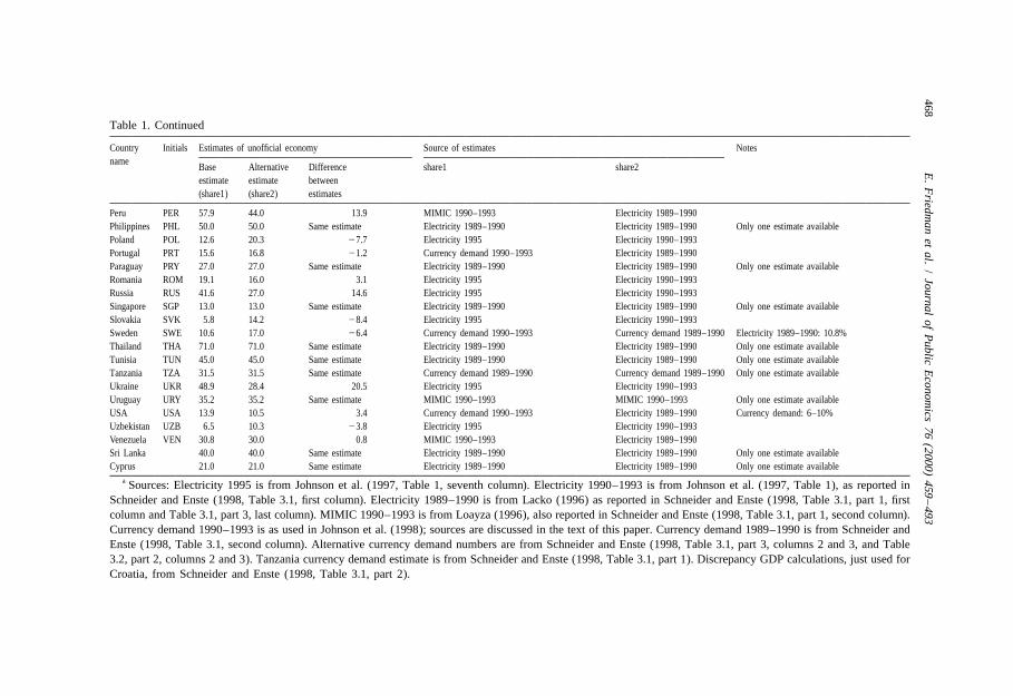
Peru PER 57.9 44.0 13.9 MIMIC 1990–1993 Electricity 1989–1990Philippines PHL 50.0 50.0 Same estimate Electricity 1989–1990 Electricity 1989–1990 Only one estimate availablePoland POL 12.6 20.3 27.7 Electricity 1995 Electricity 1990–1993Portugal PRT 15.6 16.8 21.2 Currency demand 1990–1993 Electricity 1989–1990Paraguay PRY 27.0 27.0 Same estimate Electricity 1989–1990 Electricity 1989–1990 Only one estimate availableRomania ROM 19.1 16.0 3.1 Electricity 1995 Electricity 1990–1993Russia RUS 41.6 27.0 14.6 Electricity 1995 Electricity 1990–1993Singapore SGP 13.0 13.0 Same estimate Electricity 1989–1990 Electricity 1989–1990 Only one estimate availableSlovakia SVK 5.8 14.2 28.4 Electricity 1995 Electricity 1990–1993Sweden SWE 10.6 17.0 26.4 Currency demand 1990–1993 Currency demand 1989–1990 Electricity 1989–1990: 10.8%Thailand THA 71.0 71.0 Same estimate Electricity 1989–1990 Electricity 1989–1990 Only one estimate availableTunisia TUN 45.0 45.0 Same estimate Electricity 1989–1990 Electricity 1989–1990 Only one estimate availableTanzania TZA 31.5 31.5 Same estimate Currency demand 1989–1990 Currency demand 1989–1990 Only one estimate availableUkraine UKR 48.9 28.4 20.5 Electricity 1995 Electricity 1990–1993Uruguay URY 35.2 35.2 Same estimate MIMIC 1990–1993 MIMIC 1990–1993 Only one estimate availableUSA USA 13.9 10.5 3.4 Currency demand 1990–1993 Electricity 1989–1990 Currency demand: 6–10%Uzbekistan UZB 6.5 10.3 23.8 Electricity 1995 Electricity 1990–1993Venezuela VEN 30.8 30.0 0.8 MIMIC 1990–1993 Electricity 1989–1990Sri Lanka 40.0 40.0 Same estimate Electricity 1989–1990 Electricity 1989–1990 Only one estimate availableCyprus 21.0 21.0 Same estimate Electricity 1989–1990 Electricity 1989–1990 Only one estimate available

a Sources: Electricity 1995 is from Johnson et al. (1997, Table 1, seventh column). Electricity 1990–1993 is from Johnson et al. (1997, Table 1), as reported inSchneider and Enste (1998, Table 3.1, first column). Electricity 1989–1990 is from Lacko (1996) as reported in Schneider and Enste (1998, Table 3.1, part 1, firstcolumn and Table 3.1, part 3, last column). MIMIC 1990–1993 is from Loayza (1996), also reported in Schneider and Enste (1998, Table 3.1, part 1, second column).Currency demand 1990–1993 is as used in Johnson et al. (1998); sources are discussed in the text of this paper. Currency demand 1989–1990 is from Schneider andEnste (1998, Table 3.1, second column). Alternative currency demand numbers are from Schneider and Enste (1998, Table 3.1, part 3, columns 2 and 3, and Table3.2, part 2, columns 2 and 3). Tanzania currency demand estimate is from Schneider and Enste (1998, Table 3.1, part 1). Discrepancy GDP calculations, just used forCroatia, from Schneider and Enste (1998, Table 3.1, part 2).

E. Friedman et al. / Journal of Public Economics 76 (2000) 459 –493 469

rough measure of overall economic activity; around the world, the short-runelectricity-to-GDP elasticity is usually close to one. Measured GDP by definitioncaptures only the official part of the economy, so the difference between overalland measured GDP gives an estimate of the size of the unofficial economy.Johnson et al. (1997) make further adjustments to allow for differences in theelasticity of demand across countries. Schneider and Enste (1998) also reportalternative estimates from Lacko (1996) suggesting that the unofficial economy is

13a bit smaller than estimated by Johnson et al. (1997).Our primary source of estimates for Latin America is Loayza (1996). Loayza

uses the MIMIC (multiple-indicator multiple cause) approach to estimate the sizeof the informal sector. This statistical method infers the size of the informal sector

14from both the likely causes and likely effects of the underground economy. TheMIMIC method has two steps: the first estimates a relationship between observedindicator variables and underlying causes; and the second uses the link between

15indicator variables to infer the size of the hidden economy across countries.Schneider and Enste (1998) report a second set of estimates based on Lacko’selectricity method. As Appendix A and Table 1 show in detail, there are largedifferences between these estimates and Loayza’s work, but the two series agreethat the unofficial economy in Latin America is larger than in most OECD

16countries.Our estimates of the unofficial economy share in GDP for OECD countries were

obtained primarily from two sources: Schneider (1997) and Williams and

13Lacko’s method infers the size of the shadow economy from the household consumption ofelectricity. For details see Schneider and Enste (1998, pp. 17–19). See also Lacko (1997a,b, 1999).

14As underlying causal variables, Loayza uses the highest statutory corporate income tax in thecountry, an index of government imposed restrictions on labor markets, and Political Risk Services’indices for the quality of the bureaucracy, corruption in government, and rule of law. The proxyvariables serving as indicators of the unofficial economy itself (left hand side variables in the first stageof Loayza’s procedure) are the rate of value-added tax evasion (Silvani and Grondolo, 1993) and thepercentage of the nonagricultural labor force which does not contribute to social security (World Bank,1995).

15The first step is maximum likelihood estimation applied to a reduced form in which the dependentvariable is the set of proxy indicators and the explanatory variables are the underlying causes. Thecoefficients are identified by normalizing the coefficients that relate the latent variable with one of theindicators. In order to obtain estimates of the latent unofficial economy variable, the parameters fromthe first stage regression are used in a second ‘causes’ regression (Loayza, 1998). This procedure isvery similar to estimating a relationship between observable proxy variables and underlying causes, andthen inferring the unobservable dependent variable from its relationship to the proxy variables.

16Table 1 shows there are important differences between the estimates for some important countries,such as Chile, Mexico, Russia, and Ukraine. The relative position of some Latin American and formerSoviet countries is reversed. Nevertheless, our main results are robust to our choice of data series.

470 E. Friedman et al. / Journal of Public Economics 76 (2000) 459 –493

17Windebank (1995). Both sources base their estimates on studies that assume theuse of cash is correlated with unofficial activities. For Belgium, Germany, Spain,France, Ireland, Italy and the Netherlands we used the simple average from theSchneider (1997) and Williams and Windebank (1995). For Canada and Japan the

18only estimates we could find were from Bartlett (1990). For Greece and the UK,our data are the average of the estimates by Bartlett (1990) and Williams andWindebank (1995). For Norway and Sweden we averaged estimates by Bartlett(1990) and Schneider (1997). For the United States we averaged Bartlett (1990),

19Schneider (1997), and the estimate by Cebula (1997). For three countries therewas only one available estimate: Portugal (Williams and Windebank, 1995),Switzerland (Schneider, 1997), and Austria (Schneider, 1997). Most of theseestimates are for the early 1990s. Schneider and Enste (1998) report alternativeestimates of currency demand, but the differences from our series are for the mostpart quite small (see Appendix A and Table 1).

For Africa and Asia our source is Schneider and Enste (1998). They drawprimarily on Lacko’s electricity-method, but they also add currency demand-basedestimates for Tanzania and Mexico. They also review carefully the availablequalitative and anecdotal evidence, and find that the quantitative estimates arereasonable.

3.2. Measures of policy

As measures of policy we use expert ratings of the business environmentcalculated by the Fraser Institute, the Heritage Foundation, Freedom House,Political Risk Services, Price Waterhouse, Flemings (the investment bank), and LaPorta et al. (1998). We also use results from surveys of business people conductedby the World Economic Forum’s Global Competitiveness Survey, the InternationalInstitute for Management Development (IMD), and Impulse magazine. We alsouse Transparency International’s Corruption Perception Index.

Here we briefly review the methodology of each source and country coverage.In most cases we are not able to get exactly 69 observations. We also explain what

17Williams and Windebank use data from Dallago (1990) and European Community (1990).Schneider (1997) uses the ‘currency-demand approach’, which assumes shadow transactions take placein the form of cash. The paper reports results from several authors, and when the data were notavailable for 1990 (i.e. Austria, Denmark, Germany, France, Ireland, Italy, Netherlands, Norway,Spain, Sweden, Switzerland, UK, USA) Schneider offers his own calculations. When a range wasoffered we took the average value.

18The Bartlett (1990) article does not list sources or bibliographical references.19Cebula (1997) presents Feige’s (1994) data on unreported income based on the General Currency

Ration Model (GCR). This method is based on the US government’s Internal Revenue Service (IRS)estimate of unreported income for 1973 as an appropriate benchmark, and it also assumes that 75% ofunreported transactions are effected in cash and the rest in checkable deposits.

E. Friedman et al. / Journal of Public Economics 76 (2000) 459 –493 471

each index measures. The sample size and range of each variable are discussed inmore detail when we present the regression results.

The Fraser Institute has measured dimensions of ‘economic freedom’ at 5-yearintervals since 1975 for all the countries in our sample, except Azerbaijan, Belarus,Georgia, Kazakhstan, Moldova, and Uzbekistan (Gwarney and Lawson, 1997). Weuse four of their data series for 1995. Their taxation variable measures the topmarginal tax rate and the income threshold at which it applies. ‘Price controls’measures the extent to which businesses are free to set their own prices. ‘Freedomto compete’ measures the ability of businesses to compete in the marketplace.They also rate the equality of citizens under the law and access to a nondis-criminatory judiciary.

The Heritage Foundation surveys economic freedom every year. We use theirratings from the 1997, 1996 and 1995 Indices of Economic Freedom (Johnson andSheehy, 1995, 1996; Holmes et al., 1997). Five Heritage Foundation indices arerelevant for our study. ‘Taxation’ measures the tax rates on corporate profits,income, ‘and other significant activities’. ‘Regulation’ measures whether a licenseis required to operate a business and how easy it is to obtain such a license. It alsomeasures whether there is corruption within the bureaucracy. The assessmentincludes both average and marginal rates, as well as a view of how the tax systemis administered. ‘Property rights’ measures the protection of private propertyagainst the government and all forms of expropriation.

Freedom House surveys political freedom around the world every year(Karatnycky, 1996). In addition, it provided a review of ‘economic freedom’around the world in 1996 (Messick, 1996). This freedom ranking is the sum of sixdifferent factors according to expert opinion — the freedom to own property, earna living, operate a business, invest one’s earnings, trade internationally, andparticipate equally in all aspects of the market economy. In contrast to the HeritageFoundation and the Fraser Institute, Freedom House puts more weight on freetrade unions, ability of firms to compete against government-linked companies,

20and how easily government can suspend the right to do business.All the countries in our basic sample are covered by the Freedom House civil

liberties measure. This measure is based on expert opinion regarding the correctanswers to 13 questions regarding different dimensions of civil liberties. FreedomHouse averages the answers to obtain an overall score.

We use two indices from Political Risk Services: their ‘law and order tradition’index and ‘corruption’ index. Both measures are based on expert opinions,primarily obtained from qualitative data (Political Risk Services, no date, 1997).

The Global Competitiveness Survey (GCS) is a questionnaire answered byabout 3500 managers in 59 countries during 1996–1997 (World Economic Forum,1996, 1997). The respondents are local firms serving domestic market, local firms

20Thus Singapore does very well on the Heritage Foundation and Fraser Institute measures, but muchless well on the Freedom House measure.

472 E. Friedman et al. / Journal of Public Economics 76 (2000) 459 –493

exporting and investing abroad, and foreign firms which have made directinvestment in that country. Each question asks about one aspect of the businessenvironment and respondents provide a rating of the country on a scale of 1(poorest rating) to 7 (perfect rating). We use data from three questions. The firstasks whether government regulations impose ‘a heavy burden on businesscompetitiveness’. The second asks respondents to rate government regulationsfrom ‘vague and lax’ to ‘precise and fully enforced’. The third asks how commonare ‘irregular, additional payments connected with import and export permits,business licenses, exchange controls, tax assessments, police protection or loanapplications’.

We also use data on responses to the bribery question in the 1996 GlobalCompetitiveness Survey. This differs from the 1997 survey through having asample of 49 countries and fewer respondents (about 2000). The original ratingsscale is from 1 to 6. Most importantly, the question asked addresses corruptionmore generally, while the 1997 survey asked more specifically about incidences ofbribery closer to their experience.

The Transparency International (1998) index summarizes the results of amaximum of seven survey-based sources per country, of which we use one directly(as described above): Political Risk Services. The other five are surveys conductedby: Political and Economic Risk Consultancy Ltd., Hong Kong; Gallup Interna-tional; DRI/McGraw-Hill Global Risk Service (two surveys); the World Competi-tiveness Report from IMD, and an internet survey conducted by Johann GrafLambsdorff (1998) at Gottingen University, Germany. To be included in theTransparency International published measure, a country must have had at leastfour polls.

One further measure of bribery is a survey of German business peopleconducted in 1992–1994 by Peter Neumann and his colleagues at Impulse (aGerman business publication) (Neumann, 1994). Respondents were typicallyexporters conducting frequent business with at least one of 103 countries. We useresponses to the question about the prevalence of bribes in securing contracts for aparticular country. On average 10 people were interviewed for each country, witha minimum of three exporters per country.

For taxation, we use data from Price Waterhouse about the level of personalincome tax rates, corporate income tax rates, the VAT (or equivalent) rate, and thesocial security tax rate on employees and employers (Price Waterhouse, 1997a,b).We also use data from the Institute for International Management (IMD) on therights and responsibilities of shareholders, government transparency, and theextent to which the bureaucracy hinders business. In 1998, IMD surveyed 4314firms in 46 countries to compile these measures (IMD, 1998). For measures ofcorporate governance and shareholder rights, we rely on Flemings (1998) and onLa Porta et al. (1998).

3.3. Instrumental variables

Our model implies an important simultaneity between the quality of economic

E. Friedman et al. / Journal of Public Economics 76 (2000) 459 –493 473

institutions on the one hand and the share of the unofficial economy on the other.For example, if the model is correct, more over-regulation increases diversion ofresources underground, but this diversion reduces government revenue andundermines economic institutions such as the rule of law. To deal with this issue,we use the set of instrumental variables developed by La Porta et al. (1999).

La Porta et al. (1999) have five sets of variables that can be used as instruments.La Porta et al. (1999, Table 2) use these variables to explain institutionaldevelopment. We use their independent variables in our first stage regression (i.e.as instruments).

Firstly, they measure ethnolinguistic fractionalization. Secondly, they report theshare of each country’s population that is Catholic, Muslim, Protestant or other.These fractions sum to 100, and we follow La Porta et al. (1998) in using theProtestant proportion as our base category. Thirdly, they calculate the origin ofcommercial laws. There are five possible origins: English, French, Scandinavian,German, and socialist. La Porta et al. (1998) code five dummy variables, each ofwhich equals one if a country belongs to a particular legal system and zerootherwise. Every country belongs to at least one system. We use the English

21system as our base case. The final instrument is the geographical location ofcountries, as measured by the absolute value of countries’ latitudes.

4. Results

To make our results easier to understand, in the main text we present a summaryof our results and some key robustness tests. Appendix B presents regressionsusing alternative independent variables and also a more complete set of robustnesschecks, including instrumental variables estimation. We summarize these results inthe main text but look in detail only at one variable representing each of the fourcategories of independent variable: tax rates, over-regulation, legal environment,and corruption.

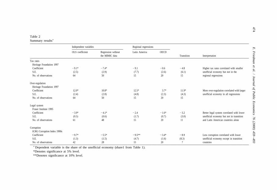
Table 2 reports OLS results for one variable representing each category ofindependent variable. It also shows the effects of dropping the MIMIC data fromLoayza (1996). We also show the effects of running the same regression just forthree regions: Latin America, OECD, and transition countries. The Latin Americandata are primarily from the MIMIC method, the OECD data are primarily fromcurrency demand estimates, and the transition countries’ data are primarily fromelectricity data. These regional regressions are therefore also checks on the effectsof using different methodologies. We unfortunately do not have enough data onAfrica or Asia to run separate regressions for those regions.

21We use legal origin only as an instrument in this paper. We are therefore just concerned that it beexogenous with respect to the unofficial economy in the 1990s. We are not concerned here with exactlyhow legal origin came about or what it really represents.

474E

.F

riedman

etal.

/Journal

ofP

ublicE

conomics

76(2000)

459–493

Table 2aSummary results

Independent variables Regional regressions

OLS coefficient Regression without Latin America OECDthe MIMIC data Transition Interpretation

Tax ratesHeritage Foundation 1997Coefficient 29.1* 27.4* 29.1 20.6 24.8 Higher tax rates correlated with smallerS.E. (2.5) (2.9) (7.7) (2.6) (6.1) unofficial economy but not in theNo. of observations 64 50 15 20 15 regional regressions

Over-regulationHeritage Foundation 1997Coefficient 12.0* 10.8* 12.5* 3.7* 11.9* More over-regulation correlated with largerS.E. (2.4) (2.8) (4.8) (2.3) (4.3) unofficial economy in all regressionsNo. of observations 64 50 15 20 15

Legal systemFraser Institute 1995Coefficient 23.9* 24.1* 22.4 21.6* 23.2 Better legal system correlated with lowerS.E. (0.5) (0.6) (1.7) (0.7) (3.0) unofficial economy but not in transitionNo. of observations 61 48 15 20 11 and Latin American countries alone

CorruptionICRG Corruption Index 1990sCoefficient 29.7* 25.5* 29.5** 23.4* 28.9 Less corruption correlated with lowerS.E. (1.3) (1.5) (4.7) (1.6) (8.3) unofficial economy except in transitionNo. of observations 42 28 15 20 7 countriesa Dependent variable is the share of the unofficial economy (share1 from Table 1).*Denotes significance at 5% level.**Denotes significance at 10% level.

E. Friedman et al. / Journal of Public Economics 76 (2000) 459 –493 475

4.1. Tax rates

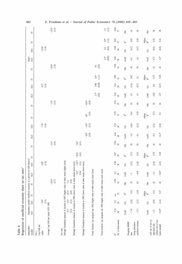
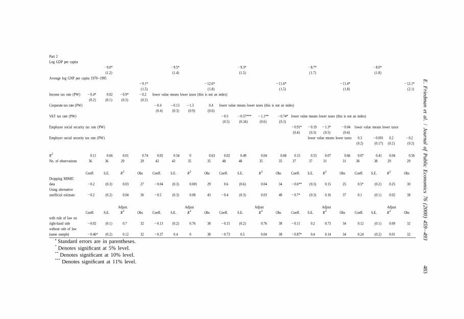
We have information on eight measures of tax rates from three independentsources. The full set of unofficial economy regressions using this data are in Table4.

Here we focus on the Heritage Foundation measure of 1997 tax rates, in which ahigher score (on a scale of 1 to 5) means more onerous taxation, i.e. higher

22average and marginal tax rates. Note that OECD countries typically have a scorethat is higher than that for transition economies and for Latin America. Forexample, in 1997 the US scores 3.5, UK scores 4, and Italy scores 5, while amongthe transition economies Georgia scores 2.5, Russia scores 3.5, and Ukraine scores4.5 and in Latin America, Brazil scores 2.5 and Argentina scores 3.5. In otherwords, according to this measure the US has higher marginal and average tax ratesthan does Russia. Tables 2 and 4 show that this measure of taxation is significantin 1997 (and in 1995). However, higher tax rates are correlated with a lower shareof the unofficial economy. Raising taxation by one point, according to thismeasure, implies that the share of the unofficial economy falls by 9.1%.Controlling for log GDP per capita reduces the coefficient by about half in all 3years but it remains significant (see Table 4). In the instrumental variablesregression (Table 4), the coefficient on the taxation variable is negative andsignificant (except when we control for log income in 1997).

Table 2 shows that dropping the MIMIC data does not change the finding thathigher tax rates are correlated with a small unofficial economy — the coefficient inthe regression (second column of Table 2) falls to 27.4 but remains significant atthe 5% level. However, the tax rate variable is not significant in any of the threeregional regressions. This may be due to insufficient observations, but it is alsopossible that the tax rate result in the main regression is caused by cross-region(and cross-methodology) variation.

Summarizing the complete results in Appendix B, higher tax rates are generallycorrelated with a lower share of the unofficial economy. This is true if we use taxrates directly or if we use an index representing the effective tax burden. Richercountries have both higher tax rates and a smaller unofficial economy. Across thecountries in our sample, the incentive to go underground to dodge higher tax ratesis outweighed by the benefits of remaining official when tax rates are higher. Thisis probably because, at least for this set of countries, higher tax rates generaterevenue that provides productivity enhancing public goods and a strong legal

23environment.

22This index is an average of income taxes and corporate taxes, adjusted for other taxes such asvalue-added taxes, sales taxes, and state and local taxes. They analyze both the top income tax rate andthe rate that applies to the average taxpayer.

23The last two rows of Table 4 show the effects of introducing ‘law and order’ (representing the levelof public goods provision) into the taxation regressions. Any tax variable that is significant in the OLSregression using the same sample becomes insignificant when we introduce this control for the legalenvironment.

476 E. Friedman et al. / Journal of Public Economics 76 (2000) 459 –493

4.2. Over-regulation

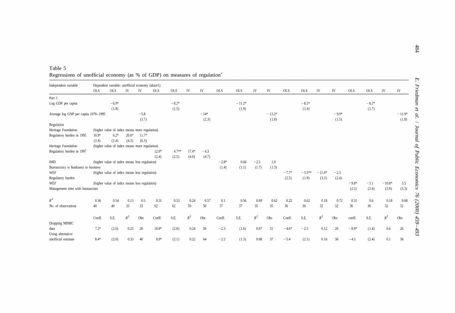
The Heritage Foundation’s measure of over-regulation is higher, on a scale of 1to 5, for countries that have regulations that are worse for business. We use thisindex for 1995 (Table 5) and also for 1997 (in Table 2). In 1995, the CzechRepublic and Britain have the best score — they are the only countries in oursample to get a perfect 1. Most OECD countries score 2. A number of EastEuropean and Latin American countries score 4 (out of a possible 5). Table 2shows that a one-point increase in this index is associated with a 12.0% increase in1997. Table 5 shows that controlling for log GDP per capita reduces the coefficienton the over-regulation variable, to 6.2 in 1995 and to 4.7 in 1997, but in both casesit remains significant (although only at the 10% level in 1997). The over-regulation indices for 1995 and 1997 are also significant in the instrumentalvariable regressions (Table 5).

Again Table 2 shows that dropping the MIMIC data does not change this resultsubstantially — the coefficient falls to 10.8 and stays significant at the 5% level.The over-regulation variable is also significant in all three of the regionalregressions, even though we only have 15 observations for both Latin America andthe transition countries.

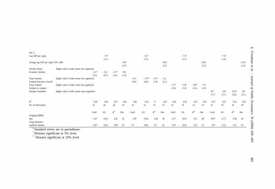
Summarizing the results in the appendix, every available measure of over-regulation is significantly correlated with the share of the unofficial economy andthe sign of the relationship is unambiguous: more over-regulation is correlated

24with a larger unofficial economy. For all but one of our variables, the coefficientin our basic instrumental variables regression is also significant. For six out of ournine measures, the correlation is significant even once we control for log per capitaincome. Overall, this is strong evidence that, across countries, more over-regula-tion is associated with more unofficial activity.

It is important to point out the difference between regulation and over-regulation. The measures we are using, such as that of Freedom House, explicitlyfocus on the ‘pro-business’ character of the state and thus include strong rules with

25respect to the preservation of property rights and contract enforcement. We findthat more over-regulation is correlated with more unofficial activity.

This does not imply that sensible regulation, for example concerning pollutionor health and safety at work, necessarily are associated with more unofficialactivity. At present, we do not have sufficient data to test this point thoroughly, butthe anecdotal evidence suggests that many such regulations can be productivity-enhancing when implemented in a sensible manner. This is a topic for furtherresearch.

24When we drop the MIMIC data from Loayza (1996), eight out of nine of these measures remainsignificant. The exception is IMD’s measure of whether the bureaucracy is a hindrance to business (seeTable 5).

25We are grateful to a referee for making this distinction clear to us.

E. Friedman et al. / Journal of Public Economics 76 (2000) 459 –493 477

4.3. Legal environment

In the Fraser Institute measure of ‘Equality of Citizens under the Law andAccess of Citizens to a Non-Discriminatory Judiciary’, a higher score means a

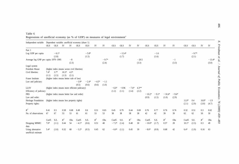
26‘better’ legal system, on a scale of 0 to 10. We have this data for 61 countries inour sample. Only Belgium, Holland, Sweden, Norway, Denmark and Switzerlandget the top score of 10. Italy, UK and USA score 7.5. Russia scores 2.5 and Brazilscores 0. Table 2 shows that a one-point increase in this index (i.e. animprovement in the legal system) implies a 3.9 percentage point fall in theunofficial economy’s share of total GDP. Controlling for log GDP per capitareduces the coefficient to 2.4 but it remains significant at the 5% level (Table 6).This variable is significant in the basic instrumental variables regression, but notonce we control for income.

Dropping the MIMIC data actually increases the coefficient to 24.1 (Table 2).The legal system variable is not significant in the Latin America or transitionregressions, but it is significant in the OECD regression.

In summary, the results in the appendix show a weaker legal environment isstrongly correlated with a larger share of the unofficial economy in GDP. All fiveof our legal environment measures are significant in the basic OLS and IVregressions and three of them remain significant when we control for log GDP percapita in both the OLS and IV cases. The results for shareholder rights are muchweaker: two out of three measures are significant, although only at the 10% level,and only one is significant in an IV regression. Creditor rights do not appear to besignificantly correlated with the unofficial economy, although it is just possiblethat stronger creditor rights might be associated with a larger unofficial economy.

4.4. Corruption

The Political Risk Services index for the 1990s has data on 42 countries. Thisindex runs from 1 to 6, with a higher score still representing less corruption, and inthis case the most corruption is reported to be in Paraguay, followed closely byseveral other Latin American countries. A one-point increase in this index iscorrelated with a 9.7% fall in the share of the unofficial economy. Controlling forlog GDP per capita reduces the coefficient to 6.4, but it remains significant at the

25% level; the R rises from 0.6 to 0.64. In this case, the variable is significant inboth the IV regressions.

Dropping the MIMIC data reduces the coefficient to 25.5 but it remainssignificant at the 5% level (Table 2). This corruption variable is significant in both

26The questions asked are: are citizens equal under the law, with access to an independent,nondiscriminatory judiciary and are they respected by the security forces? The original source isFreedom House, Survey of Political Rights and Civil Liberties 1995–96, item 5 on their checklist of 13civil liberties, with some adjustments.

478E

.F

riedman

etal.

/Journal

ofP

ublicE

conomics

76(2000)

459–493

Table 3aRegression of tax revenues on taxation, regulation, legal environment, and corruption

Independent Dependent variable

variableRevenue/ Revenue/ Revenue/ Revenue/ Revenue/ Revenue/ Revenue/ Revenue/ Revenue/ Revenue /

official total official total official total official total official total

GDP GDP GDP GDP GDP GDP GDP GDP GDP GDP

Log GDP per 20.7 1.1 1.4 2.2 0.9 1.6 20.14 0.05 22 21.7

capita (1.3) (1.3) (1.5) (1.4) (1.9) (1.9) (2.5) (2.4) (1.6) (1.2)

Taxation

Heritage Foundation measure of taxation (higher value of index means higher taxes)

8.0* 8.6* 8* 7.1*

(1.5) (1.9) (1.6) (1.9)

Regulation

Heritage foundation (higher value of index means more regulation)

Regulatory burden

in 1997: 25.4* 24.1 27* 25.1*

(2.1) (2.5) (2.0) (2.3)

E.

Friedm

anet

al./

Journalof

Public

Econom

ics76

(2000)459

–493479

Legal environment

Freedom house (higher value of index means worse civil liberties)

Civil liberties: 22.5* 21.9* 23.1* 22.1

(1.1) (1.7) (1.0) (1.6)

Corruption

Transparency International (higher value of index means less corruption)

1.2** 1.3 1.8* 1.8

(0.7) (1.2) (0.6) (1.2)

Overall

Unofficial economy (higher value denotes larger share of the unofficial economy in total GDP; not an index)

20.3* 20.4* 20.5* 20.6*

(0.09) (0.12) (0.07) (0.09)

2R 0.35 0.35 0.36 0.37 0.12 0.13 0.21 0.25 0.09 0.09 0.15 0.17 0.07 0.07 0.17 0.17 0.24 0.26 0.51 0.53

No. of

observations 53 53 49 49 53 53 49 49 55 55 51 51 46 46 44 44 51 51 51 51

a Standard errors are in parentheses.* Denotes significant at 5% level.** Denotes significant at 10% level.

480 E. Friedman et al. / Journal of Public Economics 76 (2000) 459 –493

the Latin American (at the 10% level) and OECD (at the 5% level) regressions. Itis not, however, significant for transition countries, probably because thisregression only has seven observations.

In summary, the relationship between share of the unofficial economy and ruleof law (including corruption) is strong and consistent across eight measuresprovided by six distinct organizations. Results from all eight of the indices shownin Table 7 suggest that countries with more corruption have a higher share of theunofficial economy. This is true for five of the indices even when we control forincome level, for eight of the indices in the basic IV regression, and for three ofthe indices in the IV regression that also controls for income.

4.5. Public finance

According to our model, higher tax rates could be correlated with either higheror lower government revenue. However, there is an unambiguous prediction forthe other three variables. Higher government revenue as a percent of GDP shouldbe correlated with less over-regulation, less corruption, and stronger legalinstitutions.

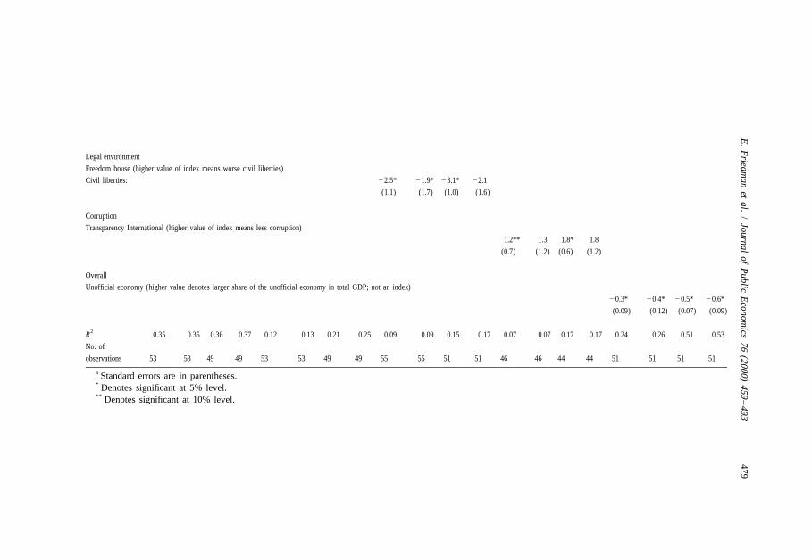
Table 3 shows regressions for two measures of tax revenue: as a percent ofofficial GDP and as a percent of total (official plus unofficial) GDP. As right-handside variables, we use one index for each of our four categories, taxation,over-regulation, legal environment, corruption. We also report results from usingthe share of the unofficial economy as a regressor. We run each regression withand without controlling for log GDP per capita.

The first four columns show that higher tax rates are actually correlated withhigher tax revenues in all specifications. A one-point increase in this taxationindex is associated with between 7 and 8.6 percentage point increase in revenue asa percent of GDP. In terms of our model, this suggests that across countries theindirect effect of tax rates on the unofficial economy dominates the direct effect,i.e. higher tax rates can generate revenue that improves the legal environmentenough to encourage activity to stay in the official sector. We would caution,however, that this does not mean that raising tax rates in any one country wouldnecessarily increase revenue and reduce unofficial activity.

The remaining columns show that more over-regulation, a weaker legalenvironment, more corruption, and a larger unofficial economy are all associatedwith less government revenue. The results are a little weaker when we control forlog GDP per capita, and the corruption variable is not significant at all in this case,but most of the coefficients are robust. The unofficial economy variable issignificant in all four specifications, implying that a one point increase in the shareof the unofficial economy means a fall in tax revenue as a percent of official GDPfrom 0.3 to 0.5% and as a percent of total GDP from 0.5 to 0.6%.

These results further support our view that weak institutions, but not high taxrates, undermine the government’s ability to collect tax revenue. Although ourevidence is cross-country rather than time series, it strongly suggests that firms

E. Friedman et al. / Journal of Public Economics 76 (2000) 459 –493 481

going underground leads to lower government revenue, and that this in turnreduces the quality of important institutions and thus increases the incentive to gounderground.

Why is bad government also small government (La Porta et al., 1999)? Wesuggest the answer lies first and foremost with the ability of firms everywhere togo underground. Going underground undermines government revenue and reducesthe provision of public goods that are important for production in the officialsector. In turn this reduces the incentive for entrepreneurs and managers to keeptheir activities in the official, taxable sector.

5. Conclusion

Higher marginal tax rates do not appear to be associated with a larger unofficialeconomy. Discretion in the application of rules, and the corruption that thisproduces, seems to have a more important effect. We find smaller unofficial sectorsin countries with a lower regulatory ‘burden’ on enterprise, less corruption, abetter rule of law, and higher tax revenue.

Both over-regulation and corruption amount to a higher effective tax on officialactivity and therefore induce firms to move into the unofficial economy. Moving tothe unofficial economy undermines public finance and further weakens the abilityof the state to protect property rights (particularly from lower level officials).

This does not imply that regulation per se drives activity underground. In fact, itis quite possible that sensible regulations, for example on health and safety atwork, contribute to higher productivity. Unfortunately, in much of the worldover-regulation by bureaucrats is a serious problem. In addition to producingcorruption and distortion, our results strongly suggest that over-regulation drivesbusiness underground and thus undermines government revenue and the sensibleprovision of productivity-enhancing public goods.

In principle, higher tax rates could be an important reason for firms to move intothe unofficial economy. In our sample, however, it appears that higher tax rates areassociated with more tax revenue, a stronger legal environment, and less unofficialactivity. We would caution, however, that a great deal depends on how the taxsystem is administered. Russia is a leading example of a country that has moderatestatutory tax rates but a corrupt system of tax administration. The way the Russiantax system is run means that there is a heavy burden on firms and many of themchoose to go underground.

Acknowledgements

We thank Norman Loayza, Friedrich Schneider, Andrei Shleifer, and a refereefor helpful suggestions. Simon Johnson gratefully acknowledges support from theMIT Entrepreneurship Center. Authors are responsible for the paper’s views,

482 E. Friedman et al. / Journal of Public Economics 76 (2000) 459 –493T

able

4a

Reg

ress

ion

ofun

offic

ial

econ

omy

shar

eon

tax

rate

s

Inde

pend

ent

Dep

ende

ntva

riabl

e:un

offic

iale

cono

my

asa

perc

ento

fG

DP

(sha

re1)

shar

e1va

riabl

eO

LSO

LSIV

IVO

LSO

LSIV

IVO

LSO

LSIV

IVO

LSO

LSIV

IVO

LSO

LSIV

IV

Part

1Lo

gG

DP

per

capi

ta2

8.0*

28.

8*2

7.9*

28.

7*2

10.8

*(1

.3)

(1.4

)(1

.8)

(1.4

)(1

.4)

Ave

rage

Log

GN

Ppe

rca

pita

1970

–199

52

10.0

*2

8.1*

27.

0*2

10.8

*2

10.5

*(2

.7)

(2.4

)(3

.3)

(1.8

)(2

.1)

Tax

rate

sH

erita

geFo

unda

tion

mea

sure

ofta

xatio

nin

1997

(hig

her

valu

eof

inde

xm

eans

high

erta

xes)

29.

1*2

4.5*

220

.1*

25.

1(2

.5)

(2.1

)(4

.6)

(5.0

)H

erita

geFo

unda

tion

mea

sure

ofta

xatio

nin

1996

(low

erva

lue

ofin

dex

mea

nslo

wer

taxe

s)2

9.2*

24.

0**

219

.4*

29.

6*(2

.6)

(2.2

)(4

.2)

(4.1

)H

erita

geFo

unda

tion

mea

sure

ofta

xatio

nin

1995

(low

erva

lue

ofin

dex

mea

nslo

wer

taxe

s)2

9.8*

25.

0*2

18*

210

.0*

(2.8

)(2

.5)

(3.9

)(4

.8)

Fras

erIn

stitu

te:t

opm

argi

nalr

ate

1995

(hig

her

valu

eof

inde

xm

eans

low

erta

xes)

2.7*

0.88

4.4*

0.9

(0.8

)(0

.69)

(1.1

)(0

.9)

Fras

erIn

stitu

te:t

opm

argi

nalr

ate

1990

(hig

her

valu

eof

inde

xm

eans

low

erta

xes)

2.1*

0.2

4.9*

1.3

(0.8

2)(0

.6)

(1.2

)(1

.1)

2R

0.18

0.5

n.a.

0.58

0.2

0.56

0.07

0.56

0.24

0.51

0.19

0.53

0.16

0.51

0.09

0.59

0.16

0.68

0.03

0.64

No.

ofob

serv

atio

ns64

6452

5250

5039

3940

4033

3358

5852

5238

3837

37

22

22

2Co

eff.

S.E.

RO

bsCo

eff.

S.E.

RO

bsCo

eff.

S.E.

RO

bsCo

eff.

S.E.

RO

bsCo

eff.

S.E.

RO

bsD

ropp

ing

MIM

ICda

ta2

7.4*

(2.9

)0.

1250

25

(3.2

)0.

1336

21.

6(3

.6)

0.01

261.

8(1

.0)

0.07

452

0.2

(0.7

)0.

0324

Usin

gal

tern

ativ

eun

offic

iale

stim

ate

27.

1*(2

.1)

0.16

642

8.4*

(1.8

)0.

3250

29.

1(2

.1)

0.33

401.

9(0

.7)

0.1

591.

9(0

.7)

0.19

38

Adj

ust.

Adj

ust.

Adj

ust.

Adj

ust.

Adj

ust.

22

22

2Co

eff.

S.E.

RO

bsCo

eff.

S.E.

RO

bsCo

eff.

S.E.

RO

bsCo

eff.

S.E.

RO

bsCo

eff.

S.E.

RO

bsw

ithru

leof

law

onrig

ht-h

and

side

21.

5(2

.0)

0.12

422

1.1

(1.8

)0.

7642

20.

3(2

.3)

0.73

362

0.02

0.6

0.75

422

0.71

(0.5

)0.

7938

with

outr

ule

ofla

w(s

ame

sam

ple)

211

.8*

(2.4

)0.

3742

210

.6*

(2.6

)0.

2842

211

.2*

(2.8

)0.

336

3.5*

(0.7

)0.

3842

2.2*

(0.8

)0.

1638

E.

Friedm

anet

al./

Journalof

Public

Econom

ics76

(2000)459

–493483

Part 2Log GDP per capita

29.0* 29.5* 29.3* 28.7* 28.0*(1.2) (1.4) (1.5) (1.7) (1.8)

Average log GNP per capita 1970–199529.1* 212.6* 211.6* 211.4* 212.1*

(1.5) (1.8) (1.5) (1.8) (2.1)Income tax rate (PW) 20.4* 0.02 20.9* 20.2 lower value means lower taxes (this is not an index)

(0.2) (0.1) (0.3) (0.2)Corporate tax rate (PW) 20.4 20.13 21.3 0.4 lower value means lower taxes (this is not an index)

(0.4) (0.3) (0.9) (0.6)VAT tax rate (PW) 20.5 20.57*** 21.1** 20.74* lower value means lower taxes (this is not an index)

(0.5) (0.34) (0.6) (0.3)Employee social security tax rate (PW) 20.91* 20.19 21.3* 20.04 lower value means lower taxes

(0.4) (0.3) (0.5) (0.4)Employer social security tax rate (PW) lower value means lower taxes 0.3 20.001 0.2 20.2

(0.2) (0.17) (0.2) (0.2)

2R 0.11 0.66 0.01 0.74 0.02 0.54 0 0.63 0.02 0.49 0.04 0.68 0.15 0.53 0.07 0.66 0.07 0.41 0.04 0.56No. of observations 36 36 29 29 43 43 35 35 48 48 35 35 37 37 31 31 38 38 29 29

2 2 2 2 2Coeff. S.E. R Obs Coeff. S.E. R Obs Coeff. S.E. R Obs Coeff. S.E. R Obs Coeff. S.E. R ObsDropping MIMICdata 20.2 (0.3) 0.03 27 20.04 (0.3) 0.001 29 0.6 (0.6) 0.04 34 20.6** (0.3) 0.15 25 0.5* (0.2) 0.25 30Using alternativeunofficial estimate 20.2 (0.2) 0.04 36 20.5 (0.3) 0.08 43 20.4 (0.3) 0.03 48 20.7* (0.3) 0.16 37 0.1 (0.1) 0.02 38

Adjust. Adjust Adjust Adjust Adjust2 2 2 2 2Coeff. S.E. R Obs Coeff. S.E. R Obs Coeff. S.E. R Obs Coeff. S.E. R Obs Coeff. S.E. R Obs

with rule of law onright-hand side 20.02 (0.1) 0.7 32 20.13 (0.2) 0.76 38 20.15 (0.2) 0.76 38 20.11 0.2 0.73 34 0.12 (0.1) 0.69 32without rule of law(same sample) 20.46* (0.2) 0.12 32 20.37 0.4 0 38 20.73 0.5 0.04 38 20.87* 0.4 0.14 34 0.24 (0.2) 0.01 32

a Standard errors are in parentheses.* Denotes significant at 5% level.** Denotes significant at 10% level.*** Denotes significant at 11% level.

484E

.F

riedman

etal.

/Journal

ofP

ublicE

conomics

76(2000)

459–493

Table 5aRegressions of unofficial economy (as % of GDP) on measures of regulation

Independent variable Dependent variable: unofficial economy (share1)OLS OLS IV IV OLS OLS IV IV OLS OLS IV IV OLS OLS IV IV OLS OLS IV IV

Part 1Log GDP per capita 26.9* 28.2* 211.2* 28.5* 28.2*

(1.8) (1.5) (1.9) (1.4) (1.7)Average log GNP per capita 1970–1995 25.8 214* 213.2* 29.9* 211.9*

(3.7) (2.3) (1.8) (1.5) (1.8)RegulationHeritage Foundation (higher value of index means more regulation)Regulatory burden in 1995 10.9* 6.2* 20.0* 11.7*

(2.4) (2.4) (4.3) (6.3)Heritage Foundation (higher value of index means more regulation)Regulatory burden in 1997 12.6* 4.7** 17.4* 24.3

(2.4) (2.5) (4.0) (4.7)IMD (higher value of index means less regulation) 22.8* 0.66 22.5 1.9Bureaucracy is hindrance to business (1.4) (1.1) (1.7) (1.3)WEF (higher value of index means less regulation) 27.7* 23.5** 211.0* 22.3Regulatory burden (2.5) (1.9) (3.3) (2.4)WEF (higher value of index means less regulation) 29.8* 23.1 210.8* 3.5Management time with bureaucrats (2.5) (2.4) (3.9) (3.3)

2R 0.36 0.54 0.13 0.5 0.31 0.53 0.24 0.57 0.1 0.56 0.09 0.62 0.22 0.62 0.18 0.72 0.31 0.6 0.18 0.68No. of observations 40 40 33 33 62 62 50 50 37 37 35 35 36 36 32 32 36 36 32 32

2 2 2 2 2Coeff. S.E. R Obs Coeff. S.E. R Obs Coeff. S.E. R Obs Coeff. S.E. R Obs coeff. S.E. R ObsDropping MIMICdata 7.2* (2.6) 0.25 26 10.8* (2.8) 0.24 50 22.3 (1.6) 0.07 31 24.6* 22.5 0.12 26 28.9* (1.4) 0.6 26Using alternativeunofficial estimate 8.4* (2.0) 0.33 40 8.9* (2.1) 0.22 64 22.2 (1.3) 0.08 37 25.4 (2.1) 0.16 36 24.5 (2.4) 0.1 36

E.

Friedm

anet

al./

Journalof

Public

Econom

ics76

(2000)459

–493485

Part 2Log GDP per capita 27.3* 28.1* 27.3* 27.6*

(2.1) (1.5) (1.5) (1.4)Average log GNP per capita 1970–1995 29.6* 28.6* 210.6* 212.0*

(2.7) (2.5) (2.2) (2.2)Freedom House (higher value of index means less regulation)Economic freedom: 22.1* 20.4 24.7* 20.8

(0.5) (0.7) (1.0) (1.3)Fraser Institute (higher value of index means less regulation) 24.1* 21.5** 29.1* 23.2Freedom from price controls: (0.9) (0.9) (1.8) (2.1)Fraser Institute (higher value of index means less regulation) 25.7* 22.8* 29.0* 21.4Freedom to compete: (1.0) (1.0) (1.6) (1.9)Heritage Foundation (higher value of index means more regulation) 10* 4.9* 13.8* 0.6

(1.7) (1.7) (2.6) (3.1)

2R 0.29 0.44 0.27 0.65 0.28 0.52 0 0.61 0.36 0.55 0.25 0.63 0.37 0.57 0.33 0.63No. of observations 45 45 34 34 61 61 53 53 61 61 53 53 62 62 50 50

2 2 2 2Coeff. S.E. R Obs Coeff. S.E. R Obs Coeff. S.E. R Obs Coeff. S.E. R ObsDropping MIMICdata 22.0* (0.4) 0.42 35 25.8* (0.8) 0.42 48 26.1* (0.9) 0.51 48 10.9* (1.7) 0.48 49Using alternativeunofficial estimate 20.8* (0.4) 0.09 45 23* (0.8) 0.2 62 24.6* (0.9) 0.32 62 6.9* (1.5) 0.25 63

a Standard errors are in parentheses.* Denotes significant at 5% level.** Denotes significant at 10% level.

486E

.F

riedman

etal.

/Journal

ofP

ublicE

conomics

76(2000)

459–493

Table 6aRegressions of unofficial economy (as % of GDP) on measures of legal environment

Independent variable Dependent variable: unofficial economy (share 1)OLS OLS IV IV OLS OLS IV IV OLS OLS IV IV OLS OLS IV IV OLS OLS IV IV

Part 1Log GDP per capita 26.1* 25.8* 212.4* 21.6 29.7*

(1.8) (1.5) (1.7) (1.6) (2.1)Average log GNP per capita 1970–1995 28 29.7* 220.5 21 213.4*

(2.3) (2.4) (3.3) (3.3) (3.0)Legal systemFreedom House (higher index means worse civil liberties)Civil liberties: 7.4* 3.7* 10.3* 4.3*

(1.1) (1.5) (1.3) (2.1)Fraser Institute (higher index means better rule of law)Law and judiciary: 23.9* 22.4* 24.5* 21.1

(0.5) (0.6) (0.6) (1.0)LLSV (higher index means more efficient judiciary) 26.6* 20.96 27.6* 4.3**Efficiency of judiciary: (1.2) (1.1) (1.4) (2.2)PRS (higher index means better law and order) 210.2* 29.1* 210.4* 29.6*Law and order: (0.9) (1.5) (1.0) (2.9)Heritage Foundation (higher index means less property rights) 11.0* 0.4 16.8* 21.9Property rights: (2.1) (2.9) (3.0) (4.7)

2R 0.41 0.5 0.58 0.68 0.49 0.6 0.51 0.65 0.45 0.79 0.44 0.69 0.76 0.77 0.76 0.76 0.32 0.51 0.3 0.62No. of observations 67 67 53 53 61 61 53 53 38 38 38 38 42 42 39 39 62 62 50 50

2 2 2 2 2Coeff. S.E. R Obs Coeff. S.E. R Obs Coeff. S.E. R Obs Coeff. S.E. R Obs Coeff. S.E. R ObsDropping MIMIC 7.0* (1.1) 0.44 54 24.1* (0.6) 0.51 48 27.2* (1.4) 0.48 30 210.0* (1.7) 0.57 28 10.1* (2.3) 0.3 49dataUsing alternative 5.4* (1.0) 0.32 68 23.2* (0.5) 0.45 62 26.0* (1.1) 0.45 39 28.0* (0.9) 0.68 42 6.4* (1.9) 0.16 63unofficial estimate

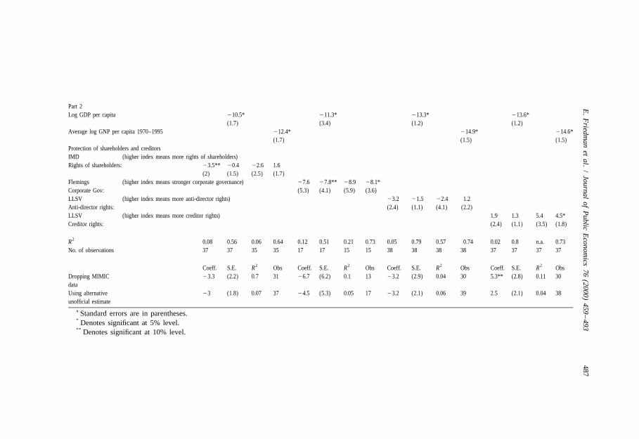
E.

Friedm

anet

al./

Journalof

Public

Econom

ics76

(2000)459

–493487

Part 2Log GDP per capita 210.5* 211.3* 213.3* 213.6*

(1.7) (3.4) (1.2) (1.2)Average log GNP per capita 1970–1995 212.4* 214.9* 214.6*

(1.7) (1.5) (1.5)Protection of shareholders and creditorsIMD (higher index means more rights of shareholders)Rights of shareholders: 23.5** 20.4 22.6 1.6

(2) (1.5) (2.5) (1.7)Flemings (higher index means stronger corporate governance) 27.6 27.8** 28.9 28.1*Corporate Gov: (5.3) (4.1) (5.9) (3.6)LLSV (higher index means more anti-director rights) 23.2 21.5 22.4 1.2Anti-director rights: (2.4) (1.1) (4.1) (2.2)LLSV (higher index means more creditor rights) 1.9 1.3 5.4 4.5*Creditor rights: (2.4) (1.1) (3.5) (1.8)

2R 0.08 0.56 0.06 0.64 0.12 0.51 0.21 0.73 0.05 0.79 0.57 0.74 0.02 0.8 n.a. 0.73No. of observations 37 37 35 35 17 17 15 15 38 38 38 38 37 37 37 37

2 2 2 2Coeff. S.E. R Obs Coeff. S.E. R Obs Coeff. S.E. R Obs Coeff. S.E. R ObsDropping MIMIC 23.3 (2.2) 0.7 31 26.7 (6.2) 0.1 13 23.2 (2.9) 0.04 30 5.3** (2.8) 0.11 30dataUsing alternative 23 (1.8) 0.07 37 24.5 (5.3) 0.05 17 23.2 (2.1) 0.06 39 2.5 (2.1) 0.04 38unofficial estimate

a Standard errors are in parentheses.* Denotes significant at 5% level.** Denotes significant at 10% level.

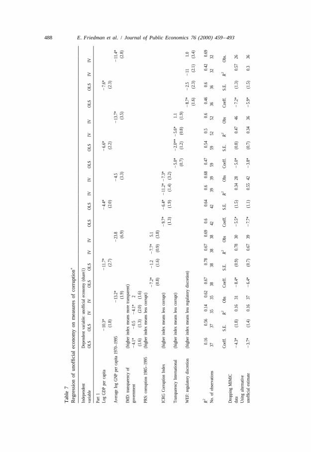
488 E. Friedman et al. / Journal of Public Economics 76 (2000) 459 –493

Tab

le7

aR

egre

ssio

nof

unof

ficia

lec

onom

yon

mea

sure

sof

corr

uptio

n

Inde

pend

ent

Dep

ende

ntva

riabl

e:un

offic

ial

econ

omy

(sha

re1)

varia

ble

OLS

OLS

IVIV

OLS

OLS

IVIV

OLS

OLS

IVIV

OLS

OLS

IVIV

OLS

OLS

IVIV

Part

1Lo

gG

DP

per

capi

ta2

10.3

*2

11.7

*2

4.4*

26.

6*2

7.6*

(1.8

)(2

.7)

(2.0

)(2

.2)

(2.3

)A

vera

gelo

gG

NP

per

capi

ta19

70–1

995

213

.2*

223

.82

4.5

213

.7*

211

.4*

(1.9

)(6

.9)

(3.3

)(3

.5)

(2.8

)IM

D:

trans

pare

ncy

of(h

ighe

rin

dex

mea

nsm

ore

trans

pare

nt)

gove

rnm

ent

24.

1*2

0.5

24.

1*2

(1.6

)(1

.3)

(2.0

)(1

.6)

PRS:

corr

uptio

n19

85–1

995

(hig

her

inde

xm

eans

less

corr

upt)

27.

2*2

1.2

27.

7*5.

1(0

.8)

(1.6

)(0

.9)

(3.8

)IC

RG

Cor

rupt

ion

Inde

x(h

ighe

rin

dex

mea

nsle

ssco

rrup

t)2

9.7*

26.

4*2

11.2

*2

7.3*

(1.3

)(1

.9)

(1.4

)(3

.2)

Tran

spar

ency

Inte

rnat

iona

l(h

ighe

rin

dex

mea

nsle

ssco

rrup

t)2

5.0*

22.

0**

25.

6*1.

1(0

.7)

(1.2

)(0

.8)

(1.9

)W

EF:

regu

lato

rydi

scre

tion

(hig

her

inde

xm

eans

less

regu

lato

rydi

scre

tion)

28.

7*2

2.5

211

1.0

(1.6

)(2

.3)

(2.1

)(3

.4)

2R

0.16

0.56

0.14

0.62

0.67

0.78

0.67

0.69

0.6

0.64

0.6

0.68

0.47

0.54

0.5

0.6

0.46

0.6

0.42

0.69

No.

ofob

serv

atio

ns37

3735

3538

3838

3842

4239

3959

5952

5236

3632

32

22

22

2C

oeff

.S.

E.R

Obs

Coe

ff.

S.E.

RO

bsC

oeff

.S.

E.R

Obs

Coe

ff.

S.E.

RO

bsC

oeff

.S.

E.R

Obs

.D

ropp

ing

MIM

ICda

ta2

4.3*

(1.8

)0.

1631

28.

4*(0

.9)

0.78

302

5.5*

(1.5

)0.

3428

25.

0*(0

.8)

0.47

462

7.2*

(1.3

)0.

5726

Usi

ngal

tern

ativ

eun

offic

ial

estim

ate

23.

7*(1

.4)

0.16

372

6.4*

(0.7

)0.

6739

27.

7*(1

.1)

0.55

422

3.8*

(0.7

)0.

3436

25.

9*(1

.5)

0.3

36

E.

Friedm

anet

al./

Journalof

Public

Econom

ics76

(2000)459

–493489

Part 2Log GDP per capita 26* 26.5* 25.3*

(2.4) (2.1) (1.9)Average log GNP per capita 1970–1995 27.6* 26.4* 24.6

(3.2) (2.4) (3.7)WEF: bribery in 1997 (higher index means less bribery)

27.6* 23.5** 28.7* 22.8(1.2) (2.0) (1.3) (2.7)

WEF: bribery in 1996 (higher index means less bribery) 24.7* 22.2** 25.6* 22.8*(0.9) (1.1) (1.1) (1.4)

Neumann Foundation: corruption (higher index means more corrupt) 1.9* 1.1* 2.3* 1.4**(0.33) (0.4) (0.33) (0.8)

Impulse’s (higher index means more corrupt) 7.2* 4.0* 8.3* 4.9***Exporter Bribery Index (1.2) (1.6) (1.2) (2.9)

2R 0.54 0.62 0.55 0.71 0.49 0.62 0.45 0.65 0.42 0.51 0.53 0.65 0.42 0.51 0.53 0.66No. of observations 36 36 32 32 30 30 28 28 48 48 36 36 48 48 36 36

2 2 2 2Coeff. S.E. R Obs Coeff. S.E. R Obs Coeff. S.E. R Obs Coeff. S.E. R ObsDropping MIMICdata 26.3* (1.3) 0.51 26 23.8* (0.7) 0.57 23 1.8* (0.4) 0.34 37 6.5* (1.5) 0.34 37Using alternativeunofficial estimate 25.6* (1.1) 0.43 36 23.0* (0.8) 0.33 30 12* (0.3) 0.32 48 4.4 (0.9) 0.32 48

a Standard errors are in parentheses.* Denotes significant at 5% level.** Denotes significant at 10% level.*** Denotes significant at 11% level.

490 E. Friedman et al. / Journal of Public Economics 76 (2000) 459 –493

errors and omissions; in particular we would stress that the views expressed hereare those of the authors alone.

Appendix A. Unofficial economy estimates

Our baseline estimates (denoted share1 in Table 1) are the same as those used inJohnson et al. (1998) and use three sets of sources. For developed countries, weuse estimates based on currency demand 1990–1993 (explained in the text above);for transition countries, we use the Johnson et al. (1997) estimates for 1995; andfor Latin America we use the MIMIC estimates for 1990–1993 from Loayza(1996). For share1 we supplement this information for Asia and Africa withestimates using Lacko’s (1996) electricity method, as reported in Schneider andEnste (1998).

Our alternative estimates (denoted share2 in Table 1) are picked to be higher forcountries with good regulatory systems and lower for countries with badregulatory systems (i.e. more over-regulation). However, rather than changingindividual values on an ad hoc basis, we instead use alternative sets of estimates.For Latin America, where available we use the electricity-based estimates ratherthan the MIMIC estimates. For transition economies, we use electricity-based

27estimates for 1990–1993 rather than for 1995. For most developed countries weuse the electricity-based method for 1989–1990 (from Lacko (1996), as reportedin Schneider and Enste (1998)), rather than currency demand estimates.

A.1. Consistency of estimates

Multiple estimates based on currency demand are available for most developedcountries. As Table 1 shows, these agree quite closely for most countries.

Electricity-based estimates, using the Lacko (1996), method are also availablefor most developed countries. In most cases these numbers are similar to thecurrency demand-based estimates. The largest differences are for Sweden andSpain. For Sweden the electricity estimate is 10.8%, while for currency demandfor 1989–1990 it is 17% (although for currency demand 1990–1993 it is 10.6%).For Spain the electricity estimate is 23.9%, while for currency demand 1990–1993it is 17.3% (but for currency demand 1996–1997 the estimate is 23%).

For nine Latin American countries there are both MIMIC and electricity-basedestimates available. The average difference between these estimates is 12.6percentage points. In four cases the electricity based estimate is higher

27Schneider and Enste (1998) report 1989–1990 and 1990–1993 averages from Johnson et al.(1997). The 1989–1990 numbers are low because communism still existed in most of these countries.For the former Soviet Union, the 1990–1993 estimates are also low relative to what happened later, butthey provide a reasonable lower bound.

E. Friedman et al. / Journal of Public Economics 76 (2000) 459 –493 491

(Guatemala, Mexico, Costa Rica, and Chile), and in five cases the MIMIC estimateis higher (Panama, Peru, Brazil, Colombia, and Venezuela). The largest differenceis for Panama, where the MIMIC estimate of 62.1% is 22.1 percentage pointshigher than the electricity-based estimate, and the smallest difference is forVenezuela where MIMIC gives 30.8% and the electricity method gives 30.0%.

No currency demand-based estimates are available for Australia, Finland, thetransition economies, or any developing countries (except Tanzania and Mexico).For 15 countries we only have a single estimate based on the electricity-method ofLacko (1996) and for 18 transition countries we only have estimates for 1989–1995 from Johnson et al. (1997). However, as Schneider and Enste (1998) discussin detail, these estimates fit well with the available single country and anecdotalevidence.

Appendix B. Alternative measures of independent variables

In order to make it easier to check our results, we have kept the original signson variables. The reader should be careful because organizations’ ratings differ inwhether a high numerical value corresponds to ‘better’ policies for business andprivate investment (i.e. less over-regulation or lower taxation). To help understandthe scaling for each variable, in addition to the regression results we reportindividual highest and lowest scores in our sample, as well as the numbers forparticularly noteworthy individual cases (Tables 4–7)

More discussion of these regression results was in our unpublished workingpaper and is available from the authors.

References

Bartlett, B., 1990. The underground economy: Achilles heel of the state? Economic Affairs 10, 24–27.Cebula, R.J., 1997. An empirical analysis of the impact of government tax and auditing policies on the

size of the underground economy: the case of the United States, 1973–1994. The American Journalof Economics and Sociology 56 (2), 73–186.

Dallago, B., 1990. The Irregular Economy: the ‘Underground’ Economy and the ‘Black’ Labor Market,Dartmouth Publishing Company, Aldershot, Hants, UK.

Delong, B., Shleifer, A., 1993. Princes and merchants: government and city growth before theIndustrial Revolution. Journal of Law and Economics 36, 671–702.

Easterly, W., Levine, R., 1997. Africas growth tragedy: policies and ethnic divisions. Quarterly Journalof Economics 112, 1203–1250.

De Soto, H., 1989. The Other Path, Harper and Row, New York.European Community, 1990. Underground Economy and Irregular Forms of Employment, Final

Synthesis Report, Office for Official Publications of the European Community.Feige, E.L., 1994. The underground economy and the currency enigma public finances. Finances

Publiques 49 (4), 119–136.Flemings Research, 1998. Global Emerging Markets, Flemings.

492 E. Friedman et al. / Journal of Public Economics 76 (2000) 459 –493

Friedman, E., Johnson, S., 1999. Looting and propping in weak legal environments, MIT, Mimeo.Gwarney, J., Lawson, R. (Eds.), 1997. Economic Freedom of the World, 1997 Annual Report, The

Fraser Institute, Vancouver.Holmes, K.R., Johnson, B.T., Kirkpatrick, M., 1997. Index of Economic Freedom, Heritage Founda-

tion, Washington, DC.IMD, 1998. The World Competitiveness Yearbook, Institute for International Management, Lausanne,

Switzerland.Johnson, B.T., Sheehy, T., 1995. The Index of Economic Freedom, Heritage Foundation, Washington,

DC.Johnson, B.T., Sheehy, T., 1996. Index of Economic Freedom, Heritage Foundation, Washington, DC.Johnson, S., Kaufmann, D., Shleifer, A., 1997. The Unofficial Economy in Transition, Brookings

Papers on Economic Activity, Washington, DC.Johnson, S., Kaufmann, D., Zoido-Lobaton, P., 1998. Regulatory discretion and corruption. American

Economic Review, May 88 (2), 387–392.Johnson, S., Boone, P., Breach, A., Friedman, E., 2000. Corporate governance in the Asian financial

crisis, 1997–98. Journal of Financial Economics, forthcoming.Karatnycky, A. (Ed.), 1996. Freedom in the World: The Annual Survey of Political Rights and Civil

Liberties 1995–1996, Freedom House, New York.Kaufmann, D., 1997. The missing pillar of a growth strategy for Ukraine. In: Cornelius, P., Lenain, P.

(Eds.), Ukraine: Accelerating the Transition to Market, IMF, Washington, DC.Kaufmann, D., Kaliberda, A., 1996. Integrating the unofficial into the dynamics of post-socialist

economies. In: Kaminsky, B. (Ed.), Economic Transition in the Newly Independent States, M.E.Sharpe Press, Armonk, New York.

Knack, S., Keefer, P., 1995. Institutions and economic performance: cross-country tests usingalternative institutional measures. Economics and Politics 7, 207–227.

Lacko, M., 1996. Hidden Economy in East-European Countries in International Comparison,International Institute for Applied Systems Analysis (IIASA), Laxenburg.

Lacko, M., 1997a. The Hidden Economies of Visegrad Countries in International Comparison: AHousehold Electricity Approach, Institute of Economics, Hungary.

Lacko, M., 1997b. Do power consumption data tell the story? (Electricity Intensity and the HiddenEconomy in Post-Socialist Countries), International Institute for Applied Systems Analysis (IIASA),Laxenburg.

Lacko, M., 1999. Hidden economy — an unknown quantity? Comparative analysis of hiddeneconomies in transition countries in 1989–1995, Johannes Kepler Universitat Linz, Sozial- UndWirtschaftswissenschaftliche Fakultat, Institut fur Volkswirtschaftslehre, Working paper 9905.

La Porta, R., Lopez-de-Silanes, F., Shleifer, A., Vishny, R.W., 1998. Law and finance. Journal ofPolitical Economy.

La Porta, R., Lopez-de-Silanes, F., Shleifer, A., Vishny, R.W., 1999. The quality of government. TheJournal of Law, Economics, and Organization 15 (1), 222–279.

Loayza, N.V., 1996. The economics of the informal sector: a simple model and some empirical evidencefrom Latin America. Carnegie-Rochester Conference Series on Public Policy 45, 129–162.

Loayza, N.V., 1998. Private communication.Lambsdorff, J.G., 1998. Paper presented at Lima (Peru) International Anti-corruption Conference

(IAC).Mauro, P., 1995. Corruption and growth. Quarterly Journal of Economics 110, 681–712.Messick, R.E., 1996. World Survey of Economic Freedom, 1995–1996, Freedom House, New York.

¨Neumann, P., 1994. Bose: Fast Alle Bestechen (Flaunting the Rules: Almost Everybody). Impulse,January 4.

Political Risk Services (PRS), no date. International Country Risk Guide (ICRG), A Business Guide toPolitical Risk.

Political Risk Services, 1997. Private communication.Price Waterhouse, 1997a. Individual Taxes: A Worldwide Summary, Price Waterhouse, New York.

E. Friedman et al. / Journal of Public Economics 76 (2000) 459 –493 493

Price Waterhouse, 1997b. Corporate Taxes: A Worldwide Summary, Price Waterhouse, New York.Schneider, F., 1997. Empirical results for the size of the shadow economy of western European

countries over time, Johannes Kepler Universitat Linz (Austria). Institut fur Volkswirtschaftslehre,Working paper, no. 9710:1-22; March.

Schneider, F., Enste, D., 1998. Increasing shadow economies all over the world — fiction or reality: asurvey of the global evidence of its size and of its impact from 1970 to 1995, IMF and University ofLinz, August 21.

Shleifer, A., 1997. Schumpeter lecture: government in transition. European Economic Review, April47, 385–410.

Silvani, C., Grondolo, J., 1993. An analysis of VAT compliance, Fiscal Affairs Department,International Monetary Fund, Mimeo.

Transparency International, 1998. Corruption Perception Index, Transparency International.Williams, C.C., Windebank, J., 1995. Black market work in the European Community: peripheral work

for peripheral localities? International Journal of Urban and Regional Research 19 (1), 23–39.Wilson, D., 1996. Acer Computer in Russia, Fuqua School of Business, Duke University.World Bank, 1995. Averting the Old Age Crisis, World Bank, Washington DC.World Economic Forum, 1997. Executive Survey, 1997, World Economic Forum, Geneva.World Economic Forum, 1996. Global Competitiveness Report, World Economic Forum, Geneva.