1

Does Auditor Industry Specialization Improve Audit Quality?

Evidence from Comparable Clients

Miguel Minutti-Meza*

m.minuttimeza06@rotman.utoronto.ca

University of Toronto

Rotman School of Management

November 2010

ABSTRACT: The objective of this study is to examine the relation between auditor industry

specialization and audit quality using an alternative research design to mitigate the influence of

client characteristics. After matching clients of specialist and non-specialist auditors according to

industry, size and performance, I find no significant differences in audit quality between these two

groups of auditors. My findings are robust to using alternative matching approaches, to using

various proxies for auditor industry specialization and audit quality, and to controlling for the effect

of imperfectly matched characteristics. In addition, I perform two analyses that do not rely primarily

on matched samples. First, in examining a sample of Arthur Andersen clients that switched auditors

in 2002, I find no evidence of industry-specialization effects following the auditor change. Second, I

observe that the industry-specialization effects are simulated by randomly assigning clients to

auditors. Overall, these findings do not imply that industry knowledge is not important for auditors,

but that the extant methodology may not fully parse out the effects of auditor industry expertise

from client characteristics.

* This paper is based on the first chapter of my dissertation at the University of Toronto, Rotman School of

Management. I gratefully acknowledge the guidance provided by my co-chairs Gordon Richardson and Ping Zhang,

as well as the other members of my dissertation committee, Jeffrey Callen and Gus De Franco. I thank Yiwei Dou,

Stephanie Larocque, Alastair Lawrence, Yanju Liu, Matthew Lyle, Ole-Kristian Hope, Yu Hou, Dushantkumar Vyas,

and seminar participants at the University of Toronto, and the 2010 CAAA PhD Consortium, for helpful comments

and suggestions. I also acknowledge the financial support of the Canadian Public Accountability Board. All errors

are my own.

2

I. INTRODUCTION

Accounting firms recognize the importance of industry expertise in providing high-quality

audits and organize their assurance practices along industry lines. In large firms, individual

auditors specialize by auditing clients in the same industry. For example, PwC highlights that

“our audit approach, at the leading edge of best practice, is tailored to suit the size and nature of

your organisation and draws upon our extensive industry knowledge (PwC 2010).” A report on

the U.S. audit market issued by the U.S. General Accounting Office (GAO) in 2008 also

acknowledges the importance of industry expertise, noting that “a firm with industry expertise

may exploit its specialization by developing and marketing audit-related services which are

specific to clients in the industry and provide a higher level of assurance (GAO 2008; p. 111).”

Asserting the benefits of auditor industry specialization is relevant for public companies choosing

among auditors, to regulators concerned with high concentration on the U.S. audit market, and to

audit firms aiming to perform high-quality audits while maintaining their competitive position in

each industry.1

Auditing researchers have extensively studied the consequences of auditor expertise.

Experimental auditing research confirms the importance of auditor expertise by providing

evidence that knowledge of the industry may increase audit quality, improving the accuracy of

error detection (Owhoso et al. 2002; Solomon et al. 1999), enhancing the quality of the auditor’s

risk assessment (Low 2004; Taylor 2000), and influencing the choice of audit tests and the

1 Since four audit firms hold the majority of the U.S. audit market for public companies, specialization may lead to

dominance of a single audit firm within an industry. Dominance by a single audit firm in an industry may have

undesirable consequences such as high audit fees and low audit quality. Extant research shows that auditors may be

able to obtain a specialization fee premium by improving efficiency and creating barriers to entry. Francis et al.,

(2005) find an association between fee premiums and joint national and city specialist auditors in the U.S. audit

market; DeFond et al. (2000) find a specialization premium in addition to audit quality effects the Hong Kong audit

market; however, Carson and Fargher (2007), focusing on the Australian audit market, find that the association

between the specialist fee premium and auditor specialization is concentrated in audit fees paid by the largest clients

in each industry.

3

allocation of audit hours (Low 2004). Empirical auditing research has also examined the effects

of auditor industry expertise; however, empirical researchers cannot directly observe expertise at

the firm, office, or auditor level, and this area of the literature has used each audit firm’s within-

industry market share, or auditor industry specialization, as an indirect proxy for auditor industry

expertise. A specialist is a firm that has “differentiated itself from its competitors in terms of

market share within a particular industry” (Neal and Riley 2004; p. 170). Previous studies that

use within-industry market share proxies for industry specialization have shown that the clients

of specialist auditors have better financial reporting quality, exhibiting on average from 0.3 to 2.0

percent lower absolute discretionary accruals, compared to clients of non-specialist auditors

(Balsam et al. 2003; Krishnan 2003; Reichelt and Wang 2010).

Measuring the effects of auditor industry expertise on audit quality is problematic because

the proxies for industry specialization and audit quality are associated with underlying client

characteristics. For example, large clients have lower absolute discretionary accruals and large

clients are often audited by industry specialists. For determining causal inference in observational

studies, empirical researchers should aim to compare treated and control groups that have similar

client characteristics, ideally approximating experimental conditions. A potential way to achieve

this objective is by matching treatment and control observations on all relevant observable

dimensions except for the treatment and outcome variables. This study proposes a methodology

to find economically comparable clients and applies it to mitigate the effect differences in client

characteristics between specialists and non-specialist auditors.

Controlling for confounding factors is particularly important in studying the effects on

industry specialization for two main reasons. First, an audit firm may have extensive industry

knowledge even when its within-industry market share is small relative to other audit firms.

4

Industry knowledge could be gained through other means; for instance, by the number of years an

audit team has audited clients in the industry, by providing training to individual auditors, by

auditing private clients in the same industry, by providing consulting services, and by hiring

experts from within the industry or from other audit firms.2 Thus, it is not obvious that auditors

with larger market share will have higher quality. Second, the evidence in Boone et al. (2010) and

Lawrence et al. (2010) shows that the previously documented association between auditor size

and audit quality could be attributed to differences in client characteristics, particularly to

differences in client size. The separation of specialist and non-specialist auditors by within-

industry market share also creates two groups of auditors with different client characteristics. For

example, specialist auditors have larger and more profitable clients compared to non-specialist

auditors.

Prior studies of auditor industry specialization control for the impact of client

characteristics by including client size, performance, growth, and other linear control variables in

multivariate regression analyses. There are two problems with the linear control approach:

important variables such as client size and performance are nonlinear to both the auditor choice

decision and the proxies for audit quality (Kothari et al. 2005; Hribar et al. 2009; Lawrence et al.

2010), and differences in client characteristics are partially a result of endogenous self-selection.

Furthermore, previous research by Rubin (1979), Heckman et al. (1998), Rubin and Thomas

(2000), and Rubin (2001), shows that linear regression may increase bias in the estimation of

treatment effects when there are even moderately nonlinear relationships between the dependent

and independent variables, and this problem is exacerbated when there are significant differences

2 For example, a recent article in Bloomberg’s BusinessWeek notes that “Deloitte recruiters say they're doing better

head-to-head against such old-shoe firms as McKinsey and BCG Consulting, both in recruiting and getting new

business” and that this firm “typically gets more than 85 percent of the experienced hires it makes an offer to”

(Byrnes 2010).

5

in means and variances in the independent variables between treated and control groups. To

overcome the endogeneity problem, some studies use econometric designs that explicitly model

the mechanism that results on differences in client characteristics between auditors, such as the

Heckman (1979) self-selection model or two-stage models. A limitation of these research designs

is that they require identifying appropriate exogenous instrumental variables or exclusion

restrictions in the first stage, which is a difficult condition to meet in models predicting auditor

choice (Francis et al. 2010). Moreover, two-stage models may perform poorly when there is

insufficient overlap between treatment and control observations (Glazerman et al. 2003; Dehejia

and Wahba 2002). The matching models used in this study constitute an alternative to determine

the auditor treatment effects. 3

Consistent with previous studies, I first document the relation between audit quality and

auditor industry specialization at the U.S. national and city level in my full sample analyses.

Throughout my analyses, I use three audit-quality proxies: discretionary accruals, a revenue

manipulation proxy from Stubben (2009), and the auditor’s propensity to issue a going-concern

opinion. The main matching approach used in this study is based on three fundamental economic

dimensions: industry, size, and performance. After matching clients of specialist and non-

specialist auditors, I find no significant differences in audit quality between the two groups of

auditors. My findings are robust to using alternative matching approaches, to using various

proxies for auditor industry specialization and audit quality, and to controlling for the effect of

imperfectly matched characteristics.

3 Heckman (2005) discusses extensively the advantages and disadvantages of matching versus explicit modelling of

the selection process. Both approaches are acceptable for estimating treatment effects; however, the matching

approach does not require identification of exclusion restrictions. Conversely, matching relies on the assumption that

selection is strictly based on observables or that treatment assignment is “strongly ignorable,” and also requires some

degree of overlap or “common support” between treatment and control observations. I discuss the implications of

this assumption for my research design in Section II.

6

I also document confirmatory evidence from two additional analyses. First, I find

statistically insignificant pre-post differences in discretionary accruals or revenue manipulation

for Arthur Andersen’s clients that exogenously switched to auditors with a different degree of

specialization in 2002. Second, using a simulation procedure, I assign clients to five simulated

auditors at random and designate specialist and non-specialist auditors based on within-industry

market share. I observe that the auditor that is assigned the largest clients of the industry is often

designated as specialist, and that specialist auditors appear to have higher audit quality compared

to non-specialist auditors, highlighting the confounding effect of client size on tests of auditor

industry specialization.

In sum, the combined evidence provided in this study suggests that the extant empirical

methodology may not fully parse out the confounding effects of client characteristics in tests of

auditor industry specialization and audit quality. I caution that my findings do not imply that

industry knowledge is not important for auditors. Furthermore, my results are subject to the

intrinsic limitations of matching for estimating causal effects, resulting from a trade-off between

internal and external validity, and to the proxies for audit quality and auditor industry

specialization used in this study. Finally, beyond the audit literature, this study contributes to the

broad accounting literature on matching and economic comparability. The methodology used here

could be adapted to other studies in accounting research comparing treated and control groups,

particularly where it is difficult to specify a correct model or to find exogenous predictors of

treatment choice.4

4 For example, a study using discretionary accruals as a dependent variable and a treatment variable correlated with

firm size and performance (e.g., management compensation, corporate governance, or financial analyst following)

may benefit from using the methodology applied in this study.

7

II. AUDIT QUALITY AND ECONOMIC COMPARABILITY

Peer-Matching and economic comparability

Using peer-firms as a benchmark is common among practitioners and researchers. Peer-

firms are used by financial analysts to support their price-earnings ratios, earnings forecasts, and

overall stock recommendations (Bradshaw et al. 2009; De Franco et al. 2009), by investment

managers in structuring their portfolios (Chan et al. 2007), by compensation committees in

setting executive compensation (Albuquerque 2009), by business valuators in determining

valuation multiples (Bhojraj et al. 2002), and by auditors in applying analytical procedures

(Hoitash et al. 2006). In using peer-firms as benchmarks, practitioners rely on comparability or

uniformity of financial information and on the overall quality of the mapping of economic events

into financial reporting. Several prior studies in accounting research have used peer-matching “as

a research design device for isolating a variable of particular interest” (Bhojraj et al. 2002; p.

410), to simplify data collection (Geiger and Rama 2003), to provide more reliable inferences in

market-based research (Barber and Lyon 1997), and to mitigate the effect of nonlinearities

(Kothari et al. 2005).5 A primary objective of this study is to use fundamental economic

characteristics to match peer-firms in order to obtain inferences about relative accounting quality

between two groups of auditors.

Peer-matched test of audit quality

To investigate the difference in audit quality between two auditors, researchers must

ascertain that the observed differences between the auditors’ clients are the result of the auditors’

5 Furthermore, other disciplines have done extensive research on the benefits and drawbacks of matching to identify

causal effects; for example, applied statistics (Stuart 2009; Rubin 2006; Rosenbaum 2002), epidemiology (Brookhart

et al. 2006), sociology (Morgan and Harding 2006), applied econometrics (Imbens 2004), and political science (Ho

et al. 2007). Zhao (2004, p.100) notes that “Selection bias due only to observables is a strong assumption. But with a

proper data set and if the selection-on-observables assumption is justifiable, matching methods are useful tools to

estimate treatment effects.”

8

effect. A peer-based approach could be useful in identifying the auditor treatment effects under

two general scenarios.

In the first scenario, assume that (1) clients do not engage routinely in earnings

management, (2) low-quality auditors allow random noise in accounting accruals as a result of

inconsistent enforcement of accounting principles, and (3) two clients are economically

comparable and have the same drivers of accounting accruals, but one client has a low-quality

auditor and the other client has a high-quality auditor. Under these ideal conditions, the only

difference between these two clients’ accruals is the random noise introduced by the low-quality

auditor.

In the second scenario, assume that (1) clients engage routinely in earnings management,

(2) low-quality auditors are not able to fully uncover earnings management, and (3) two clients

are economically comparable and have the same drivers of accounting accruals, but one client has

a low-quality auditor and the other client has a high-quality auditor. Under these conditions, the

effect of earnings management should be the only difference between these two clients’ accruals.

Along these lines, researchers may identify differences between the accruals of clients of

specialist and non-specialist auditors if specialist auditors are better at enforcing the right

accounting policies and at constraining earnings management. In a general setting where the true

accrual function is unknown, the overall difference in accrual quality between two clients can be

approximated by employing a combination of a discretionary accruals model and matching on

economic comparability. Similarly, a test of the differences in propensity to issue a going-concern

opinion between specialist and non-specialist auditors could be well specified if the matching

process mitigates differences in client characteristics that could influence the probability of

bankruptcy.

9

Matched-sample estimators of the effects of specialization

A univariate t-test of the differences in means between perfectly matched clients

constitutes a direct estimator of the specialist auditor treatment effects (Zhao 2004). However, if

the matching process is not perfect, it is still important to control for unmatched client

characteristics using multivariate analyses. I conduct multivariate analyses in all matched

samples of specialist and non-specialist auditors’ clients using two approaches. Under the first

approach, the same model estimated on the full sample is estimated in the pooled matched sample

of clients, while under the second approach, the pair-wise differences in the dependent variables

between peer-matched clients of specialists are regressed on the pair-wise differences of the

independent variables in the original model (Rubin 1973; Imbens 2004; Cram et al. 2009). The

intercept of this pair-wise differences model is interpreted as the average difference resulting

from the specialist’s treatment effects. For the matched sample analyses of the propensity to issue

a going-concern opinion, I estimate a conditional fixed effect logistic regression based on

matched pairs of clients of specialist and non-specialist auditors with variation in going-concern

opinions (Cram et al. 2009).

Advantages and disadvantages of peer-matching approaches

An advantage of the peer-matched approach is that it imposes weak stationarity or

linearity conditions on the relation between the matched firm characteristics and the proxies for

audit quality. Although the peer-based approach reflects the relative quality between peer-firms,

idiosyncratic differences should be mitigated in large samples, allowing researchers to assess the

average treatment effects of specialist auditors. This argument is similar to that in Kothari et al.

(2005); however, this approach aims to isolate a wider set of client characteristics, beyond ROA,

from the proxies for audit quality. Another advantage of the peer-based approach is that it does

10

not require identification of exclusion restrictions. Finally, this approach is suitable for a

differences-in-differences test of the effect of auditor specialization for clients that switch

auditors as a result of an exogenous shock.

Using matched samples comes at a cost, thus three underlying threats to matching

approaches are (1) firms deemed to be economically similar may not be truly comparable, (2) the

results from matched samples may not be immediately extended to the entire population, and (3)

matching reduces sample sizes. These threats result from a trade-off between internal and

external validity. The first threat can be mitigated by verifying that matched firms have

homogenous characteristics across matched groups, by triangulating evidence from different

matching approaches, and by controlling for the effect of imperfectly matched variables. The

second threat may be mitigated by a combination of analyses including calculating bootstrap

standard errors and verifying that the matched sample results hold separately for industries where

specialization matters the most. The third threat may be mitigated by verifying that the result in

non-matched samples could be found even in random samples of equal or smaller size than the

matched samples, and aiming to get the largest possible matched samples. I document the results

of additional analyses to mitigate these threats in Section VIII.

Selection of matching variables and matching approach

There are two primary research-design choices applicable to matched samples. The first

choice is the set of variables or dimensions used for matching; the second is the mechanism to

aggregate across dimensions and to find comparable observations. The choice of matching

variables is important because in a strict sense, matching assumes that bias is only due to

observables. The source of bias is the difference between observables in the treatment and control

groups. The bias due to non-matched characteristics decreases as the number of matching

11

variables increases. On the other hand, the complexity and structure of the methods needed to

aggregate across dimensions increases as the number of matching variables increases.

When the number of matching variables is small, the researcher can directly match on the

variables of interest or within a specified distance from each variable of interest without requiring

a weighting approach to aggregate across dimensions. This type of matching is known as

attributes-based or covariate matching. The main approach used in this study is a form of

covariate matching. I propose that the three most important fundamental variables that affect the

audit-quality proxies and also influence the differences between auditor groups are the client’s

industry, size, and performance. The literature on discretionary accruals has repeatedly

highlighted the importance of these three dimensions and recommends estimating discretionary

accruals by industry, scaling by total assets and controlling for ROA.

To match on these dimensions, for a given fiscal year-end, industry (defined by two-digit

SIC code), and size distance (firms that are within a size distance of 50 percent), firm i is

matched to firm j with the most comparable performance, measuring performance as stock

returns’ covariance over the preceding 48 months, where higher covariance indicates higher

comparability.6 As per the De Franco et al. (2009) methodology, I measure returns covariance

using the adjusted R2 of the following regression of firm i’s monthly returns on firm j’s monthly

returns7:

RETURNSi,t = Φi,j + Φi,jRETURNSj,t + εj,t (1)

6

As noted by Chan et al. (2007, p. 57), “if equity market participants consider a set of companies closely related,

then shocks in the group of stocks should experience coincident movements in their stock returns.” 7 I also estimate Kendall’s (1938) Tau or rank correlation coefficient for my matched peer-firms. This non-parametric

statistic measures co-movement or serial dependence and can be directly interpreted as the probability of observing

concordant or discordant pairs of observations. Both correlation measures produce similar matched pairs.

12

In addition, I require matched firms to have their fiscal year-end on the same month to

reduce differences from timing in financial reporting. Allowing for 50 percent distance in total

assets results in more than one potential control for every treatment observation, and the final

selection among all possible controls is based on returns’ covariance. This procedure is likely to

closely match peer-firms deemed economically comparable by the market. Compared to other

matching approaches, it does not rely on a specific functional form to predict comparability,

beyond a returns covariance structure, and can be used not only in case-control research settings,

but also in situations where a company needs to be matched with its economic peers; for

example, to form benchmark groups for valuation or to perform analytical audit procedures.

In order to mitigate any bias resulting from imperfect matching, the pair-wise differences

analyses control for differences in size, performance and other variables between matched

observations. Furthermore, as robustness test, I also use propensity-score matching, including

several additional variables in the matching. Using propensity score, control observations are

matched to treatment observations based on a specified distance between their overall

probabilities of undergoing treatment. These probabilities are estimated using a number of

covariates that predict choice, effectively aggregating multiple dimensions into a single matching

variable. This alternative matching requires specifying a functional form for the choice model

and an acceptable distance between observations in terms of probability. I obtain similar results

either matching on the three proposed covariates or using propensity-score matching. These two

approaches are complementary in examining my main research question, and confirm that the

13

specialization effect may be attributable to differences in client characteristics. I describe the

propensity-score matching result in Section VIII.8

III. RELATED EMPIRICAL STUDIES AND MEASURES OF SPECIALIZATION

Prior studies primarily measure auditor industry specialization using the auditor’s within-

industry market share. Each auditor’s industry market share is calculated as:

I

i

J

j kij

J

j kij

ki

S

SEMARKETSHAR

ik

1 1

1 (2)

where MARKETSHAREki is the market share of auditor i in industry k, Skij represents the total

assets of client firm j in industry k audited by auditor i, J represents the number of clients that are

served by audit firm i in industry k, and I is the number of audit firms in industry k. 9

The two

main proxies for auditor industry specialization in this study are:

NLEAD1 = “1” for auditors that have the largest market share in a given industry

and year at the U.S. national level and have more than 10 percent

greater market share than the closest competitor, and “0” otherwise;

CLEAD1 = “1” for auditors that have the largest market share in a given industry

and year at the U.S. city level, where city is defined as a Metropolitan

Statistical Area following the 2003 U.S. Census Bureau MSA

definitions, and have more than 10 percent greater market share than

8 Zhao (2004) concludes that there is no clear winner between covariates and propensity-score matching methods.

When the correlation between covariates and treatment choice are high, propensity-score matching is a good choice;

however, when the sample size is small, covariate matching performs better. Hahn (1998) shows that covariate

matching is asymptotically efficient because it attains the efficiency bound, and Angrist and Hahn (2004) show that

covariate matching may be more efficient in finite samples than propensity-score matching. 9 Prior studies have also used total sales or auditor fees to compute within-industry market shares. I use total assets to

calculate my specialization measures at city and national level because total assets are available for most firms in my

sample period.

14

the closest competitor, and “0” otherwise. 10

The main analyses presented in all tables use these two proxies, and I describe similar results

using an alternative cut-off for market share and combined national and city-level specialization

proxies in Section VIII.

Balsam et al. (2003) find a negative relationship between auditor specialization and the

client’s absolute discretionary accruals. Discretionary accruals are calculated using the industry

cross-sectional Jones (1991) model and auditor industry specialization is measured using six

proxies: LEADER that equals one for auditors with the top three market shares in a given

industry, and zero otherwise; DOMINANCE that equals one for auditors that have the largest

market share in a given industry and have more than 10 percent greater market share than the

closest competitor, and zero otherwise; MOSTCL that equals one for auditors that have the most

number of clients in a given industry, and zero otherwise; SHARE that is a continuous auditor

market share variable (measured in client sales) in a given industry; SHARECL that is a

continuous auditor market share variable (measured in number of clients) in a given industry; and

NCLIENTS that is the number of clients of an auditor in a given industry.

Krishnan (2003) documents a negative relationship between auditor specialization and the

client’s absolute discretionary accruals. Discretionary accruals are calculated using the industry

cross-sectional Jones (1991) model and auditor industry specialization is measured using two

proxies: IMS1 that equals one for auditors with market share greater or equal to 15 percent in a

given industry, and zero otherwise; and IMS2 that is a continuous auditor market share variable

(measured in client sales) in a given industry.

10

Francis et al. (2005) and Reichelt and Wang (2010) also use MSA definitions to identify city-level specialists. I

delete cases when there are only two observations in a given city. MSA definitions are available at the U.S. Census

Bureau’s website: http://www.census.gov/population/www/metroareas/metrodef.html.

15

Reichelt and Wang (2010) show a negative relationship between auditor specialization

and the client’s absolute discretionary accruals. Discretionary accruals are calculated using the

industry cross-sectional Jones (1991) model, including ROA as per Kothari et al. (2005), and

auditor industry specialization is measured using two proxies at the national level, city level, and

both levels combined: SPECIALIST1 that equals one for auditors that have the largest market

share in a given industry and have more than 10 percent greater market share than the closest

competitor, and zero otherwise; and SPECIALIST2 that equals one for auditors that have over 30

percent market share in a given industry and year, and zero otherwise. In addition, this study

documents a positive association between the city-level and combined national and city-level

measures and the auditor’s propensity to issue a going-concern opinion.

Lim and Tan (2008) test the moderating effect of auditor specialization on the relationship

between non-audit fees and absolute discretionary accruals and find no statistically significant

association between absolute discretionary accruals and auditor specialization in a model without

non-audit-fee measures. At the same time, they find an interaction effect between auditor

specialization and non-audit fees, suggesting that clients audited by specialists are associated with

higher absolute levels of discretionary current accruals as non-audit fees increase. Lim and Tan

(2008) calculate discretionary accruals using the industry cross-sectional Jones (1991) model,

including ROA as per Kothari et al. (2005), and their measure of specialization equals one if the

auditor has the largest market share in the client’s industry, and zero otherwise. Furthermore, this

study documents a positive association between auditor industry specialization and the auditor’s

propensity to issue a going-concern opinion; however, the association is negative once the

specialization proxy is interacted with audit fees.

16

The studies summarized above consistently document a relationship between auditor

industry specialization and audit quality. Consistent with prior studies, I use the client’s absolute

discretionary accruals and the auditor’s propensity to issue a going-concern opinion as audit-

quality proxies. Additionally, I use a proxy for discretionary revenue, proposed by Stubben

(2010), which considers a number of cross-sectional characteristics in the estimation process.

This measure is arguably better specified at detecting revenue manipulation than the previously

used discretionary accruals measures.11

IV. AUDIT-QUALITY PROXIES AND SAMPLE SELECTION

Discretionary Accruals

As a first audit-quality proxy, I use absolute discretionary accruals, estimated using an

annual cross-sectional model for each industry. I employ two different approaches to calculate

discretionary accruals: ADA is based on a model including ROA (Kothari et al. 2005) as an

additional predictor (Equation (3) below), and ADA_FULL is based on a more comprehensive

model (Equation (4) below) including ROA (Kothari et al. 2005), cash flows in periods t and t-1

scaled by total assets (McNichols 2002), and a non-linear interaction term based on the sign of

cash flows in period t (Ball and Shivakumar 2006). In the main analyses, I use the absolute value

of discretionary accruals from the Kothari et al. (2005) model (ADA). All results are similar using

ADA_FULL, or estimating the Kothari et al. (2005) model using prior year’s ROA instead of

current year’s ROA.12

ACi,t = α + β1ΔRi,t + β2PPEi,t + β3ROAi,t + εi,t (3)

11

Table 3 in Stubben (2010, p.707) shows that this discretionary measure detects a combination of 1 percent

simulated manipulation in both revenue and expenses in 23.6 percent of the samples with manipulation, compared to

11.6 percent using the Jones model or 11.2 percent using the performance-matched modified Jones model. 12

I winsorize all variables at the 1 and 99 percent levels before estimating the discretionary accruals and

discretionary revenue models.

17

ACi,t = α + β1ΔRi,t + β2PPEi,t + β3ROAi,t + β4CFOi,t-1 + β5CFOi,t

+ β6CFOi,t+1 + β7Di,t + β8D×CFOi,t + εjt (4)

Discretionary Revenue

As a second audit-quality proxy, I use ADREV, the absolute value of discretionary

revenue, as proposed by Stubben (2010). The revenue manipulation or discretionary revenue

model (Equation (5) below) is similar to the discretionary accruals model in that it uses the

relation between changes in accounts receivable and changes in revenue to predict earnings

management. Moreover, the estimation of this measure allows for variation in the model

coefficients across client characteristics and also considers nonlinear terms, compared to

discretionary accruals models that assume the same coefficient for all clients in the same industry.

ΔARi,t = α + β1ΔRi,t+ β2ΔRi,t×SIZEi,t + β3ΔRi,t×AGEi,t + β4ΔRi,t×AGE_SQi,t

+ β5ΔRi,t×GRR_Pi,t + β6ΔRi,t×GRR_Ni,t + β7ΔRi,t×GRMi,t

+ β8ΔRi,t×GRM_SQi,t + εjt (5)

Appendix A describes the main variables of Equations (3) to (5) and the calculation of the

discretionary accruals and revenue manipulation audit-quality proxies that I use in this study.

Going-Concern Opinions

As a third audit-quality proxy, I use the auditor’s propensity to issue a going-concern

opinion. The variable for going-concern opinion (GCONCERN) is directly taken from Audit

Analytics and is coded as “1” if the auditor gave a going-concern opinion to a client in the fiscal

year, and “0” otherwise.

18

Multivariate regression models

I first replicate the findings of prior studies that test the relation between auditor

specialization and each audit-quality proxy using the following model13

:

QUALITY_PROXYi.t= ω0 + ω1LEADi,t + ω2BIG4i,t + ω3LOGMKTi,t + ω4LEVi,t

+ ω5ROAi,t+ ω6ROALi,t+ ω7LOSSi,t+ ω8CFOi,t + ω9BTMi,t

+ ω10ABS(ACCRL) i,t + ω11GROWTHi,t+ω12ALTMANi,t

+ ω13STDEARNi,t + ω14TENUREi,t + ω15YEAR F.E. + vi,t (6)

where for client i and fiscal year-end t:

QUALITY_PROXY = audit quality proxies as defined above;

LEAD = indicator variable for each measure of auditor industry specialization

as defined above (NLEAD1 or CLEAD1);

BIG4 = “1” if the client has a Big 4 auditor and “0” otherwise;

LOG_MKT = natural logarithm of market value;

LEV = (total liabilities) / average total assets;

ROA = (net income) / average total assets;

ROAL = (net incomet-1) / average total assets t-1;

LOSS = indicator variable equal one if net income is negative, and “0”

otherwise;

CFO = (cash flow from operations)/average total assets;

BTM = (book value of equity) / market value of equity;

ABS(ACCRL) = (absolute value of total accrualst-1)/average total assetst-1;

GROWTH = sales growth calculated as (sales – salest-1)/salest-1;

ALTMAN = Altman’s (1983) scores;

13

I winsorize all variables at the 1 and 99 percent levels before estimating my main models in the full samples of

each audit-quality proxy.

19

STDEARN = standard deviation of income before extraordinary items in the past

four years;

YEAR F.E. = year fixed effects.

Prior literature documents that auditor industry specialization increases audit quality and

reduces the absolute value of discretionary accruals and discretionary revenue, and it increases

the auditor’s propensity to issue a going-concern opinion. Consistent with Balsam et al. (2003)

and Reichelt and Wang (2010), lower discretionary accruals are expected for larger firms

(LOG_MKT), firms with higher operating cash flow (CFO), firms with higher leverage (LEV),

firms audited by a Big 4 auditor (BIG4), and firms with longer tenure (TENURE). Higher

absolute discretionary accruals are expected for growth firms (GROWTH and BTM), firms with

losses (LOSS), firms with extreme performance (ROA and ROAL), firms with high-income

volatility (STDEARN), firms with high probability of bankruptcy (ALTMAN), and for firms with

higher prior total accruals (ABS(ACCRL)). I expect the signs of all controls variables to be similar

in the discretionary revenue model as both proxies are influenced similarly by incentives and

opportunities for earnings management.

In the going-concern model, I expect that the probability of going concern will be lower

for larger and more stable clients (LOG_MKT, BIG4, TENURE), and decrease as liquidity (CFO,

ALTMAN) and profitability increases (ROAL, ROA). On the other hand, the probability of going

concern will increase as risk (STDREARN, ABS(ACCRL), LOSS) and leverage increases (LEV).14

14

Consistent with prior studies, the discretionary accruals and discretionary revenue models do not include industry

fixed effects because these measures are estimated by industry. My going-concern model, estimated using logistic

regression, includes both year and industry fixed effects.

20

Analysis of matched samples: pooled and pair-wise differences models

For each specialization measure, NLEAD1 and CLEAD1, I pair-match clients of specialist

and non-specialist auditors by fiscal year-end month and industry, within a 50 percent size

distance, selecting the peer with the highest stock return covariance from all the possible

matches. I estimate two alternative models using the matched samples. First, I estimate Equation

(6) in the pooled matched sample of clients of specialist and non-specialist auditors. Second, for

the discretionary accruals and discretionary revenue proxies, I estimate the following pair-wise

differences model as per Cram et al. (2009):

QUALITY_MEASUREijt= γ0 + γ1BIG4ijt + γ2LOGMKTijt + γ3LEVijt + γ4ROAijt

+ γ5ROALijt+ γ6LOSSijt+ γ7CFOijt + γ8BTMijt

+ γ9ABS(ACCRLij)t + γ10GROWTHijt+ γ11ALTMANijt

+ γ12STDEARNijt + γ13TENUREijt + γ14YEAR F.E. + ut (7)

where for fiscal year-end t, ij denotes the pair-wise difference between the value of each variable

(as previously defined) for the client of the specialist auditor minus the value of the same variable

for the matched client of a non-specialist auditor, and the intercept γ0 represents the average pair-

wise difference between matched observations, controlling for the effect of differences resulting

from imperfectly matched variables. For the going-concern audit-quality proxy, I estimate a

conditional fixed effects logistic regression, using the pair matched observations with intra-pair

variation in going concern.

21

Data and sample selection

For the discretionary accruals analyses, I use U.S. public company data for the years 1988

to 2008 from COMPUSTAT and data for the years 2000 to 2008 from Audit Analytics.15

I delete

firms in the financial services industries (SIC codes 6000–6999), firms with negative assets,

market price, or sales, and firms without the necessary data to calculate the control variables in

the main regression model. This results in a full sample consisting of 75,188 firm-year

observations with the national-level measure. The sample size is reduced to 23,307 firm-year

observations with the city-level measure. This measure is calculated for the years 2000 to 2008

with auditor city data in Audit Analytics and a corresponding city in the U.S. Census Bureau

MSA classification.

For the discretionary revenue analyses, I start with the national and city-level samples that

I use in the discretionary accruals analyses. I delete firms without the additional variables

required to calculate the discretionary revenue proxy as per Stubben (2010), in particular the

changes in accounts receivables from the statement of cash flows. This results in a full sample

consisting of 69,512 firm-year observations with the national-level measure and 21,914 firm-year

observations with the city-level measure.

For the propensity to issue going-concern analyses, I use U.S. public company data for

the years 2000 to 2008 from COMPUSTAT and auditor opinion data from Audit Analytics. I

delete firms in the financial services industries, firms with negative assets, market price, or sales,

and firms without the necessary data to calculate the control variables in the main regression

15

I restrict my analyses to this time period because reported operating cash flows, needed to calculate discretionary

accruals, are only available starting from 1988 as per SFAS No. 95 (FASB 1987).

22

model. This results in a full sample consisting of 35,406 firm-year observations with the national-

level measure and 23,349 firm-year observations with the city-level measure.16

V. RESULTS

Discretionary accruals –full-sample analyses

Table 1 presents the descriptive statistics of the full sample. Panel A shows how client

size, performance, and total accruals vary across the top eight auditors ranked by within-industry

market share at U.S. national level. I calculate the ranks by industry and year. For example, for

two-digit SIC 49, in year 2007, the auditor with the highest market share for that two-digit SIC

will be in the first rank, the auditor with the second highest will be in the second rank, and so on.

Clients of auditors with high market share are larger, have better performance, lower absolute

total accruals and lower absolute discretionary accruals and discretionary revenue. This pattern is

persistent regardless of the cut-off value used to divide specialist and non-specialist auditors.

Table 1, Panel B shows the descriptive statistics of the national-level full sample and for a

partition using NLEAD1 as measure of auditor industry specialization. Clients of national-level

specialist auditors represent 10.84 percent of the total sample, similar to the 11.6 percent reported

in Reichelt and Wang (2010, p.658). Clients of national-level specialists have on average

approximately 2 percent lower absolute discretionary accruals, are more than two times larger,

have more leverage, have lower total accruals and exhibit better performance in terms of

profitability, losses, cash flow from operations, and growth, compared to clients of non-specialist

auditors. Table 1, Panel C shows the descriptive statistics of the city-level full sample and for a

16

Some prior studies, such as Balsam et al. (2003) and Krishnan (2003), eliminate clients of the Big 4 firms from

their sample in order to get a cleaner test of specialization separate from the Big 4 effect. In order to get the largest

possible sample size, I keep clients of all firms in my main analyses, controlling for the Big 4 effect using an

indicator variable for clients of these auditors. This is consistent with Reichelt and Wang (2010).

23

partition using CLEAD1 as measure of auditor industry specialization. Clients of city-level

specialist auditors represent 33.8 percent of the total sample, similar to 35 percent in Reichelt and

Wang (2010, p.658), and the city-level partition has similar differences in characteristics

compared to the national-level partition; however, the size difference is more pronounced using

the city-level partition.

Table 2 presents the results of the full-sample analyses using NLEAD1 and CLEAD1 as

measures of auditor specialization. In line with previous studies, the coefficient on both variables

in the first two columns show that clients of specialist auditors have on average from 0.26 to 0.37

percent lower absolute discretionary accruals compared to clients of non-specialists auditors.

Discretionary accruals –matched sample analyses

Table 1, Panel B presents the descriptive statistics for the national-level matched sample

of clients of specialist and non-specialist auditors. Using NLEAD1 as measure of auditor industry

specialization, I was able to find a match for 5,479 clients of the specialist auditors within the

specified criteria. In this matched sample, clients of the specialist auditors have statistically

insignificant differences (at 1 percent level) in absolute discretionary accruals, are on average

approximately 1.2 times larger, have more leverage, and exhibit statistically weak differences (at

5 percent level) in performance in terms of profitability, losses, cash flow from operations, and

growth, compared to clients of non-specialist auditors. Other variables still exhibit statistically

significant differences, but the magnitude of the differences is considerably smaller than in the

full sample. These results show that the matching procedure balances performance and growth,

and mitigates size differences, but it does not fully mitigate differences in all variables across the

two auditor groups. Table 1, Panel C presents the descriptive statistics for the city-level matched

sample of clients of industry specialist and non-specialist auditors. Using CLEAD1 as measure of

24

auditor industry specialization, I was able to find a match for 4,979 clients of the specialist

auditors within the specified criteria. At the city level, the matching procedure is not as effective

in mitigating size and performance differences, primarily due to a different percentage of

potential control observation for each treatment observation in the full sample. In this matched

sample, there is a weakly significant difference (at 10 percent level) in mean absolute

discretionary accruals between specialist and non-specialist auditor clients; however, the

magnitude of the difference is roughly 7 percent (-0.002 compared to -0.028) of the difference in

means for the full sample.

Table 2 presents the results of the pooled matched sample analyses using NLEAD1 and

CLEAD1 as measures of auditor specialization. The coefficient on both variables, in the last two

columns, is statistically insignificant (at 1 percent level). Similarly, in Table 3, the statistically

insignificant coefficients on the intercept of the pair-wise differences regression indicate that,

controlling for unmatched characteristics between observations, there are no differences in

absolute discretionary accruals between specialist and non-specialist auditors. The combined

evidence from the univariate difference in means, pooled multivariate regressions, and pair-wise

differences regressions suggests that after controlling for differences in client characteristics

between the two auditor groups by matching, the extant research design is unable to detect

differences in absolute discretionary accruals as a result of auditor industry specialization.

Discretionary revenue –full-sample analyses

Table 4 presents the descriptive statistics of the full sample. Panel A shows the descriptive

statistics of the national-level full sample and for a partition using NLEAD1 as measure of auditor

industry specialization. Clients of national-level specialist auditors have similar proportions as

those in the discretionary accruals sample and exhibit approximately 0.8 percent lower absolute

25

discretionary revenue on average, compared to clients of non-specialist auditors. The separation

of client characteristics is very similar to those in the discretionary accruals samples. Table 4,

Panel B shows the descriptive statistics of the city-level full sample and for a partition using

CLEAD1 as measure of auditor industry specialization. Clients of city-level specialist auditors

exhibit similar characteristics as the clients of national-level specialist auditors, compared to the

clients of non-specialist auditors; however, the size difference is more pronounced in the city-

level partition than in the national-level partition.

Table 5 presents the results of the full-sample analyses using NLEAD1 and CLEAD1 as

measures of auditor specialization, the coefficient on both variables in the first two columns show

that clients of specialist auditors have on average from 0.13 to 0.2 percent lower absolute

discretionary revenue compared to clients of non-specialists auditors. These full-sample results

are consistent with the discretionary accruals full-sample results.

Discretionary revenue –matched sample analyses

Table 4, Panel A presents the descriptive statistics for the national-level matched sample

of clients of industry specialist and non-specialist auditors. Using NLEAD1 as measure of auditor

industry specialization, I find a match for 5,053 clients of the specialist auditors within the

specified criteria. In this matched sample, clients of the specialist auditors have statistically

insignificant differences (at 1 percent level) in absolute discretionary revenue. The matching

procedure balances performance and growth, mitigates size differences, but it does not fully

mitigate differences in all variables across the two auditor groups. Table 4, Panel B presents the

descriptive statistics for the city-level matched sample of clients of industry specialist and non-

specialist auditors. Using CLEAD1 as measure of auditor industry specialization, I was able to

find a match for 4,695 clients of the specialist auditors within the specified criteria. At the city

26

level, the matching procedure is not as effective at mitigating size and performance differences;

nevertheless, in this matched sample, there is a statistically insignificant difference (at 10 percent

level) in mean absolute discretionary revenue between specialist and non-specialist auditor

clients.

Table 5 presents the results of the pooled matched sample analyses using NLEAD1 and

CLEAD1 as measures of auditor specialization. The coefficient on both variables, in the last two

columns, is statistically insignificant (at 1 percent level). Similarly, in Table 6, the statistically

insignificant coefficients on the intercept of the pair-wise differences regression indicate that,

controlling for unmatched characteristics between observations, there are no differences in

absolute discretionary revenue between specialist and non-specialist auditors. These matched

sample results are in line with the discretionary accruals matched sample results.

Propensity to issue a going-concern opinion –full-sample analyses

Table 7 presents the descriptive statistics of the full sample. This sample is smaller than

the previous two samples because auditor opinion data in Audit Analytics is only available since

2000. Panel A shows the descriptive statistics of the national level full sample and for a partition

using NLEAD1 as measure of auditor industry specialization. Clients of national-level specialist

auditors have a slightly higher proportion than those in the previous two full samples and exhibit

approximately 4.3 percent incidence of going concern, compared to 10.2 percent for clients of

non-specialist auditors. This is consistent with auditor specialists having larger and more

profitable clients, which are generally less likely to go bankrupt. Table 7, Panel B shows the

descriptive statistics of the city level full sample and for a partition using CLEAD1 as measure of

auditor industry specialization.

27

Table 8 presents the results of the full-sample analyses using NLEAD1 and CLEAD1 as

measures of auditor specialization. In these analyses, only the coefficient on the city-level

measure of specialization is significant (at 1 percent level) and in the right direction, indicating

that clients of city-level specialist auditors are more likely to issue going-concern opinions.

Propensity to issue a going-concern opinion –matched sample analyses

Table 7, Panel A, presents the descriptive statistics for the national-level matched sample

of clients of industry specialist and non-specialist auditors. Using NLEAD1 as measure of auditor

industry specialization, I was able to find a match for 2,539 clients of the specialist auditors

within the specified criteria. In this matched sample, clients of the specialist auditors have

statistically insignificant differences (at 1 percent level) in incidence of going-concern opinion.

Panel B shows the city-level matched sample. Using CLEAD1 as measure of auditor industry

specialization, I was able to find a match for 4,951 clients of the specialist auditors within the

specified criteria. In this matched sample, there is a statistically insignificant difference (at 10

percent level) in incidence of going-concern opinion between clients of specialist and non-

specialist auditor clients.

Table 8 presents the results of the pooled matched sample analyses using NLEAD1 and

CLEAD1 as measures of auditor specialization. The coefficient on both variables, in the last two

columns, is statistically insignificant (at 1 percent level). In Table 9, the statistically insignificant

coefficients on the NLEAD1 and CLEAD1 conditional logistic regression indicate that,

controlling for unmatched characteristics between observations, there are no differences in

propensity to issue a going-concern opinion between specialist and non-specialist auditors. The

results of this procedure should be interpreted with caution because they are based on a small

sample of matched pairs with intra-pair variation in going-concern opinions; however, they

28

confirm the more general results from the overall difference in means between specialist and non-

specialist auditors and from the pooled logistic regression.17

After matching economically comparable clients between specialist and non-specialist

auditors, in all the matched samples, I find that the treatment effects of specialist auditors are

insignificantly different from those of non-specialist auditors with respect to absolute

discretionary accruals, absolute discretionary revenue, and auditor’s propensity to issue a going-

concern opinion.

VI. ANALYSES OF AUDITOR SWITCHES

I take advantage of the setting created by the demise of Arthur Andersen (AA), after the

firm’s indictment for obstruction of justice in 2002, to examine the changes in absolute

discretionary accruals and absolute discretionary revenue in former AA clients as a result of a

switch to a specialist auditor. Previous studies examining the result of this unique exogenous

shock find that there was a negative market reaction for AA clients during the key dates in the AA

trial (Chaney and Philipich 2002; Callen and Morel 2003), although there were some

confounding market events around the same dates (Nelson et al. 2008); that successor auditors

required more conservative accounting for former AA clients (Nagy 2005; Cahan and Zhang

2006); and that the differences pre-post switch were related to whether former AA employees

continued auditing the client after they were hired by the successor auditor in 2002 (Blouin et al.

2007). A more general study by Knechel et al. (2007) examines 318 non-AA clients that switched

auditors between 2000 and 2003, and documents that those clients who switched from non-

specialist to specialist auditors experienced statistically significant positive abnormal returns of

2.5 percent surrounding the date of the auditor change, providing additional evidence of a

17

I estimate these regressions using the Stata command clogit. Tenure, year, and industry-specific intercepts are not

included because there is insufficient intra-pair variation in these variables.

29

perceived specialist auditor effect.

In order to test whether there was a pre-post effect of a switch to a specialist auditor for

AA former clients, using each client as its own control, first I estimate the following regression

for AA clients:

ΔQUALITY_MEASUREi = δ0 + δ1ΔLEADi + δ2ΔBIG4i + δ3ΔLOGMKTi + δ4ΔLEVi

+ δ5ΔROAi+ δ6ΔROALi+ δ7ΔLOSSi+ δ8ΔCFOi + δ9ΔBTMi

+ δ10ΔABS(ACCRL) i + δ11ΔGROWTHi+ δ12ΔALTMANi

+ δ13ΔSTDEARNi + vi (8)

where Δ denotes the difference between the level of each variable (as previously defined) in 2002

and the level of that variable in 2001. In this model, the intercept δ0 represents the average

change in dependent variable controlling for changes in other characteristics, and the coefficient

δ1 on ΔLEAD represents the incremental change as a result of switching between specialist and

non-specialist auditors (ΔNLEAD and ΔCLEAD at national and city-level respectively).

To test whether there was an effect of a switch to a specialist auditor for AA former

clients, compared to a control group of economically comparable clients, for each specialization

measure, I pair-match AA and non-AA clients in 2001 by fiscal year-end month and industry,

within a 50 percent size distance, keeping the pairs with the highest stock return covariance from

all the possible matches. Using the matched sample of AA and non-AA clients, I estimate the

following pre-post regression:

ΔQUALITY_MEASUREi = ρ0 + ρ1AAi + ρ2ΔLEAD1i + ρ3AA_ ΔLEADi + ρ4ΔBIG4i

+ ρ5ΔLOG_MKT + ρ6ΔROAi+ ρ7ΔROALi+ ρ8ΔLOSSi

+ ρ9ΔCFOi + ρ10ΔBTMi + ρ11ΔABS(ACCRL) i

+ ρ12ΔGROWTHi+ ρ13ΔALTMANi + ρ14ΔSTDEARNi + zi (9)

30

where Δ denotes the level of each variable (as previously defined) in 2002 minus the level of that

variable in 2001 for all clients in the sample, and for client i

AA = “1” for AA clients and “0” otherwise; and,

AA_ΔLEAD = interaction term between AA and changes between specialist

auditors, where ΔLEAD= “-1” for clients that switched in industries

where AA was a specialist and the successor is not a specialist

auditor, ΔLEAD= “1” for clients that switched in industries where

AA was not a specialist and the successor is a specialist auditor, and

ΔLEAD= “0” for all other cases.

An advantage of this research design is that it uses an exogenous shock to test whether

specialist auditors have a direct and immediate impact on the client’s financial reporting quality.

Nevertheless, there are limitations inherent to these analyses. First, as noted by Blouin et al.

(2007), in several instances, former AA employees were hired by the successor auditors and

continued to audit the same clients. Second, there were changes in the environment that may have

motivated all auditors, specialist and non-specialist, to be more conservative in 2002. Third, the

effect of auditor specialization may not be immediately reflected in the two proxies for financial

reporting quality used in these analyses. I expect these results to be incremental to the matched

sample analyses, providing additional evidence on the shortcomings of the extant methodology to

test the association between auditor industry expertise and audit quality.

To analyze auditor switches, I use 393 AA clients that switched to a different auditor

during 2002, and for which I can estimate the discretionary accruals, discretionary revenue, and

auditor specialization proxies.18

Next, I identify clients of other auditors in 2001 that did not

switch auditors in 2002. After matching AA clients to an economically comparable group of non-

18

I do not use going-concern opinions in this analysis due to the low incidence of this variable within the clients in

my AA sample.

31

AA clients in 2001, the differences-in-differences sample has 287 AA clients and 287 non-AA

clients.

Panel A of Table 10 shows the results of the multivariate pre-post analyses for AA clients.

I do not find evidence of a pre-post change in discretionary accruals or discretionary revenue as a

result from switching between specialist and non-specialist auditors. Panel B, the differences-in-

differences results, comparing changes between 2002 and 2001 for AA and non-AA clients,

shows a weakly statistically significant coefficient (at 10 percent level) in the wrong direction for

the interaction variable AA_CLEAD1 in column three, and statistically insignificant coefficients

for this interaction term in all other columns, suggesting that there was no effect in absolute

discretionary accruals or absolute discretionary revenue from a switch between specialist and

non-specialist auditors for former AA clients. The results in Table 8 are robust to excluding

clients in industries where AA was a specialist, and switching to a non-specialist auditor

(ΔLEAD1= -1), or clients in industries where AA was a specialist, and switching to a specialist

auditor (ΔLEAD1= 0 and LEAD1= 1). The results of the switches analyses are robust to standard

errors calculated using 1,000 bootstrap replications, mitigating the concerns that the low

statistical significance could be a result of small sample size.

VII. SIMULATION ANALYSES

Using a simulation procedure, I investigate whether the observed association between

audit quality and auditor industry specialization could be observed when clients are assigned to

five auditors at random. This simulation approach aims to examine the effectiveness of the extant

methodology to isolate the effects of client characteristics from the effects of auditor industry

32

specialization. 19

The simulation is conducted in four steps; first, each year I randomly assign all

clients in the full discretionary accruals sample, as defined in previous analyses, to five auditors

using a draw from a uniform distribution; second, I identify industry specialists using industry

market share at national level, calling this simulated variable LEAD1, based on the randomly

assigned clients; third, I estimate the main regression model (Equation 6) using this simulated

sample; and finally, I repeat the first three steps 1,000 times.

Figure 1 shows the coefficients for 1,000 iterations of the simulation procedure,

employing ADA as dependent variable and LEAD1 as measure of auditor industry specialization.

The coefficient estimate for LEAD1 is negative in 97.4 percent of the iterations and has a mean

statistically different from zero (at 1 percent level) of -0.0025. In these simulations, the auditors

that are randomly assigned a sufficient number of the largest clients in each industry are often

designated as specialists, and these auditors appear to be of higher quality compared to non-

designated specialists. Overall, the results from the simulations are suggestive that client

characteristics, particularly client size, influence the observed association between audit quality

and auditor industry specialization, and that the hypothesized causal effect can be partially

replicated by random assignment of clients to auditors. Nonetheless, there is a limitation inherent

to these analyses, the randomly assigned clients from the original full sample were actually

audited by specialist or non-specialist auditors, and the actual proportion of clients audited by

specialists is increasing as client size increases, thus the designated specialists in the simulation

have clients from both specialist and non-specialist groups.

19

This approach is similar to the one used by Carson and Fargher (2007) to assess the importance of client size to

determine audit fee premiums.

33

VIII. ADDITIONAL MATCHING ANALYSES AND SENSITIVITY TESTS

Propensity score matching

Another approach that can be used to find comparable firms is the propensity score

methodology proposed by Rosenbaum and Rubin (1983). Propensity score matching is a widely

used methodology to find a group of comparable cases and control observations to mitigate the

effect of self-selection in observational causal studies. In general, propensity score matching can

be used to pair match observations that belong to two different regimes, in the context of this

study, to find comparable clients audited by specialist and non-specialist auditors. A potential

drawback of this approach is that it depends on the specification of the choice model, known as

the “strongly ignorable treatment assignment assumption.” The main advantage of propensity-

score matching is that it’s usually effective at selecting observations that are closely matched in

the predefined covariates.

For each audit-quality proxy and specialization measure, I match clients of specialist and

non-specialist auditors using propensity scores. I predict the propensity of choosing specialist

auditors at national or city level using a logistic regression where the dependent variable is the

specialist indicator variable and the independent variables are all the control variables in the main

model, including industry and year-indicator variables (Equation (6)). I match observations by

propensity score, within common support, without replacement, using a caliper distance of 0.03,

and estimate the main model in the matched sample of clients of industry specialist and non-

specialist auditors. 20

Using this methodology, I again find that clients of the industry specialist

20

These propensity score settings are consistent with Lawrence at al. (2010) and generally result in balanced

covariates between auditor groups. I obtain similar results by reducing the caliper distance, although this reduces the

sample size further. I also use the logarithm of total assets in the propensity score calculation as a size variable,

instead of the logarithm of market value, and find the same results in my matched samples as those documented in

my main analyses. In general, the logarithm of total assets in the model results in more balanced client characteristics

34

auditors have statistically insignificant differences in absolute discretionary accruals, absolute

discretionary revenue, and incidence of going-concern opinions, compared to clients of non-

specialist auditors.

Size and industry matching

I match clients of specialist and non-specialist auditors by year, industry, and total assets

only. I match observations using propensity score, estimated using the logarithm of total assets

and industry and year indicator variables as predictors in the logistic regression, within common

support, without replacement, and using a caliper distance of 0.03. In the industry and size

matched samples, clients of the specialist auditors have statistically insignificant differences in

absolute discretionary accruals, absolute discretionary revenue, and incidence of going-concern

opinions, compared to clients of non-specialist auditors, estimated using the main model on each

matched sample.

In general, I find that the industry and size matching are successful at balancing size,

performance, and leverage between auditor groups, but are not successful at mitigating

differences in cash flow from operations and absolute accruals between auditor groups. These

results suggest that, within an industry, a close match on client size is an alternative to a close

match on returns covariance or to a match on several covariates. These alternatives might not be

equivalent in small samples where idiosyncratic differences need to be more closely matched

between the case and control groups, and for those samples researchers should aim to use the

comparability measures that produce the best possible balance between matched observations.

between auditor groups. I only observe a difference in the city-level going-concern analysis, where I observe a

statistically significant coefficient on the variable CLEAD1 (at 5 percent level) in the matched sample regression

model, using the logarithm of market value in addition to the other covariates of the propensity score model, but a

statistically insignificant coefficient (at 10 percent level) using the logarithm of total assets in addition to the other

covariates of the propensity score model.

35

Overall, companies of similar size within an industry have correlated stock returns and exhibit

similar performance, and matching clients on these criteria using alternative specifications shows

that the extant research design cannot distinguish between the clients of specialist and non-

specialist auditors.

Bootstrap, random sub-samples, and stratified samples

To mitigate concerns that the lack of significance in the matched samples analyses is not a

result of smaller sample sizes, I perform three types of sensitivity analyses. First, I estimate

bootstrap standard errors for all the matched sample models using 1,000 replications and find

similar results as those documented in the main tables. Second, for the national and city-level full

samples of the three audit-quality proxies, I draw a random sub-sample of the same size as the

matched sample and estimate the main models with bootstrap standard errors using 500

replications. I find that sample size does not affect the results for the discretionary accruals and

discretionary revenue models. For the going-concern samples, I find that the results are sensitive

to sample size due to the low incidence of going-concern opinions, equal to 9.5 percent in the full

sample. Third, I examine whether the matched sample results hold separately for industries where

auditor specialization could matter incrementally to detect earnings management or to determine

the probability of going concern. Managers could have more opportunities for manipulation in

industries with high total accruals and high volatility of earnings, and may also face higher

incentives to meet expectations in competitive or high-growth industries. Similarly, determining

the probability of going concern is difficult for low-growth industries, where competition is

intense and there is high-earnings volatility. For each industry and year in the matched samples, I

calculate the median total accruals using the variable ABS(ACCRL), median sales growth using

the variable GROWTH, median industry concentration using the Herfindahl index based on total

36

assets, and median earnings volatility using the variable STDEARN. Next, each year I rank

industries using the industry median for each of these variables and estimate the main models

separately for observations in the top and bottom quartiles. I find similar results to those

documented in the main tables using the full matched samples.

Alternative measures of auditor industry specialization

I perform all of the full and matched sample analyses using an alternative market share

cut-off for the national and city-level specialist measures, equal to “1” for auditors that have over

30 percent market share in a given industry and year, and “0” otherwise. This measure results in a

greater number of clients deemed to be audited by a specialist, and larger matched samples than

in the results shown in the main tables. Using this alternative measure, the effects of auditor

industry specialization are also statistically insignificant in the matched samples for all three

audit-quality proxies and in the pre-post switch analysis for Arthur Andersen clients. Moreover,

using this alternative measure, the coefficient on the city-level specialist variable

(CLEAD1=0.0042) for the discretionary accruals matched sample is significant (at 1 percent

level) in opposite direction, mitigating the concerns that the lack of statistical significance in the

match samples is a result of smaller sample size.

I addition, I repeat all the full and matched sample analyses using a combined measure of

city-level and national-level auditor industry specialization, equal to “1” for auditors that are

specialists at both levels in a given industry and year, and “0” otherwise. I match clients of

combined city-level and national-level experts with clients of other auditors. The effect of

combined national and city-level auditor industry specialization is statistically insignificant in the

matched samples for all three audit-quality proxies.

37

IX. CONCLUSION

To determine causal inference in observational studies, empirical researchers should aim

to compare treated and control groups that have similar client characteristics, ideally

approximating experimental conditions. A potential way to achieve this objective is by matching

treatment and control observations on all relevant observable dimensions except for the treatment

variable. This study proposes a methodology to find economically comparable clients in tests of

audit quality and applies it to mitigate the effect differences in client characteristics between

specialists and non-specialist auditors in tests of auditor industry specialization and audit quality.

I use discretionary accruals, discretionary revenue, and propensity to issue a going-

concern opinion as proxies for audit quality, and within-industry market share proxies for auditor

industry specialization at the U.S. national and city level, and after matching clients of specialist

and non-specialist auditors, I document that the previously documented association between

auditor industry specialization and audit quality may be attributable to client characteristics. I

match clients based on economic comparability, by year, industry, size, and returns covariance.

Alternatively, I also match clients using different specifications of a propensity score model.

Furthermore, I do not find evidence of a pre-post change in discretionary accruals or

discretionary revenue resulting from an exogenous switch between specialist and non-specialist

auditors for a sample of Arthur Andersen clients that changed auditors in 2002. Finally, using a

simulation approach, I find that client characteristics, particularly client size, influence the

observed association between audit quality and auditor industry specialization, and that the

hypothesized causal effect can be partially replicated by random assignation of clients to auditors.

38

The results of this study do not imply that industry knowledge does not contribute to audit

quality, but that the extant methodology does not fully capture the effects of auditor industry

expertise.

39

References

Albuquerque, A., 2009. Peer firms in relative performance evaluation. Journal of Accounting and

Economics 48 (1): 69–89.

Angrist, J., and J. Hahn. When to control for covariates? Panel asymptotics for estimates of treatment

effects. Review of Economics and Statistics 86 (1): 58–72.

Ball, R., and L. Shivakumar. 2006. The role of accruals in asymmetrically timely gain and loss

recognition. Journal of Accounting Research 44 (2): 207–242.

Balsam, S., J. Krishnan, and J. Yang. 2003. Auditor industry specialization and earnings quality. Auditing:

A Journal of Practice and Theory 22 (2): 71–97.

Barber, B. and J. Lyon. 1997. Detecting long-run abnormal stock returns: the empirical power and

specification of test statistics. Journal of Financial Economics 43 (3): 341–372.

Bhojraj, S., C. Lee, and R. Sloan. 2002. Who is my peer? A valuation-based approach to the selection of

comparable firms. Journal of Accounting Research 40 (2): 407–439.

Blouin, J., B. Murray Grein, and B. Roundtree. 2007. An analysis of forced auditor change: The case of

former Arthur Andersen clients. The Accounting Review 82 (3): 621–650.

Boone, J., I. Khurana, and K. Raman. 2010. Do the Big 4 and the Second-tier firms provide audits of

similar quality? Journal of Accounting and Public Policy (Forthcoming).

Bradshaw, M., G. Miller, and G. Serafeim. 2009. Accounting method heterogeneity and analysts’

forecasts. Working paper, University of Chicago, University of Michigan, and Harvard Business

School.

Brookhart, M., Schneeweiss, S., Rothman, K., Glynn, R., Avorn, J., and Sturmer, T. 2006. Variable

selection for propensity score models. American Journal of Epidemiology 163 (12): 1149–1156.

Byrnes, N. “Deloitte Consulting is Hiring.” Bloomberg BusinessWeek, February 2010.

http://www.businessweek.com/managing/content/feb2010/ca20100211_911815.htm

Callen, J., and M. Morel. 2003. The Enron-Andersen debacle: Do equity markets react to auditor

reputation? Finance Letters: (October): 1–5.

Cahan, S. and W. Zhang. 2006. After Enron: Auditor conservatism and ex-Andersen clients. The

Accounting Review 81 (1): 49–82.

Carcello, J., and A. Nagy. 2004. Audit firm tenure and fraudulent financial reporting. Auditing: A Journal

of Practice and Theory 23 (2): 55–69.

Carson, E., and N. Fargher. 2007. Note on audit fee premiums to client size and industry specialization.

Accounting and Finance 47 (1): 423 –446.

Chan, L., J. Lakonishok, and B. Swaminathan. 2007. Industry classifications and return comovement.

Financial Analyst Journal 63 (6): 56–70.

Chaney, P. and K. Philipich. 2002. Shredded reputation: the cost of audit failure. Journal of Accounting

Research 40 (4): 1221–1245.

Cram, D., V. Karan, and I. Stuart. 2009. Three threats to validity of choice-based and matched sample

studies in accounting research. Contemporary Accounting Research 26 (2): 477–516.

DeFond, M., J. Francis, and T.J. Wong. 2000. Auditor industry specialization and market segmentation:

Evidence from Hong Kong. Auditing: A Journal of Theory and Practice 19 (1): 49–66.

40

DeFranco, G., S.P. Kothari, and R. Verdi. 2009. The Benefits of Financial Statement Comparability.

Working Paper. University of Toronto and MIT Sloan School of Management.

Dehejia, R., and S. Wahba. 2002. Propensity score matching methods for non-experimental causal studies.

Review of Economics and Statistics 84 (1): 151–161.

Dunn, K., and B. Mayhew. Audit firm industry specialization and client disclosure quality. Review of

Accounting Studies 9 (1): 35–58.

Financial Accounting Standards Board (FASB). 1987. Statement of Cash Flows. Statement of Financial

Accounting Standards No. 95. Norwalk, CT: FASB.

Francis, J, K. Reichelt, and D. Wang. 2005. The Pricing of National and City-Specific Reputations for

Industry Expertise in the U.S. Audit Market. The Accounting Review 80 (1): 113–136.

, C. Lennox, and Z. Wang. 2010. Selection models in accounting research. Working Paper,

University of Missouri-Columbia, Hong Kong University of Science and Technology, and

Nanyang Technological University.

Geiger, M., and D. Rama. 2003. Audit fees, nonaudit fees, and auditor reporting on stressed companies.

Auditing: A Journal of Practice & Theory 22 (2): 53–69.

Glazerman, S., D. Levy, and D. Myers. 2003. Nonexperimental versus experimental estimates of earnings

impacts. Annals of the American Academy of Political and Social Science 589 (1): 63–93.

Government Accountability Office (GAO). 2008. Audits of public companies. Continued concentration in

audit market for large public companies does not call for immediate action. Washington, DC:

GAO.

Hahn, J. 1998. On the role of the propensity score in the efficient estimation of average treatment effects.

Econometrica 66 (1): 315–332.

Heckman, J. 1979. The sample bias as a specification error. Econometrica 47 (1): 153–62.

, J., H. Ichimura, and P. Todd 1998. Matching as an econometric evaluation estimator. The Review

of Economic Studies 65 (2): 261–294.

Ho, D. E., Imai, K., King, G., and Stuart, E. A. 2007. Matching as nonparametric preprocessing for

reducing model dependence in parametric causal inference. Political Analysis 15 (3): 199–236.

Hoitash, R., A. Kogan, and M. Vasarhelyi. 2006. Peer-based approach for analytical procedures. Auditing:

A Journal of Practice and Theory 25 (2): 53–84.

Hribar, P., T. Kravet, and R. Wilson. 2009. A New Measure of Accounting Quality. Working Paper.

University of Iowa and University of Texas at Dallas.

Imbens, G. W. 2004. Nonparametric estimation of average treatment effects under exogeneity: A review.

Review of Economics and Statistics 86 (1): 4–29.

Jones, J., 1991. Earnings management during import relief investigation. Journal of Accounting Research

29 (2): 193–228.

Kendall, M. 1938. A New Measure of Rank Correlation. Biometrika 30 (1-2): 81–89.

Knechel, W. R., V. Naiker, and G. Pacheco. 2007. Does auditor industry specialization matter? evidence

from market reaction to auditor switches. Auditing: A Journal of Practice and Theory 26 (1): 19–

45.

Kothari, S.P., A. Leone, and C. Wasley. 2005. Performance matched discretionary accrual measures.

Journal of Accounting & Economics 39 (1): 163–197.

41

Krishnan, G. V. 2003. Does big 6 auditor industry expertise constrain earnings management? Accounting

Horizons 17 (Supplement): 1–16.

Lawrence, A., M. Minutti-Meza, and P. Zhang. 2010. Can Big 4 versus Non-Big 4 differences in audit-

quality proxies be attributed to client characteristics? The Accounting Review. (Forthcoming).

Lim, C.Y., and H.T. Tan. 2008. Non-audit service fees and audit quality: the impact of auditor

specialization. Journal of Accounting Research 46 (1): 199–246.

Low, K.Y. 2004. The effect of industry specialization on audit risk assessments and audit planning

decisions. The Accounting Review 79: 201–209.

McNichols, M. 2002. Discussion of “The quality of accruals and earnings: the role of accruals estimation

errors.” The Accounting Review 77 (Supplement): 61–69.

Morgan, S., and D. Harding, D. 2006. Matching estimators of causal effects: Prospects and pitfalls in

theory and practice. Sociological Methods & Research 35 (1): 3–60.

Nagy, A. Mandatory audit firm turnover, financial reporting quality, and client bargaining power: the case

of Arthur Andersen. Accounting Horizons 19 (2): 51–68.

Neal, T. and R. Riley, Jr. Auditor industry specialist research design. Auditing: A Journal of Practice and

Theory 23 (2): 169–177.

Nelson, K., R. Price, and B. Roundtree. 2008. The market reaction to Arthur Andersen's role in the Enron

scandal: Loss of reputation or confounding effects? Journal of Accounting and Economics 46 (2):

279–293.

Owhoso, V.E., W.F. Messier, and J. Lynch. 2002. Error detection by industry-specialized teams during the

sequential audit review. Journal of Accounting Research 40 (3): 883–900.

PricewaterhouseCoopers (PWC). 2010. Audit and assurance services. http://www.pwc.com/gx/en/audit-

services/index.jhtml

Public Company Accounting Oversight Board (PCAOB). 2003. System of Quality Control for a CPA

Firm's Accounting and Auditing Practice. QC Section 20. New York, NY: PCAOB.

Reichelt, K. and D. Wang. National and Office-Specific Measures of Auditor Industry Expertise and

Effects on Audit Quality. (2010). Journal of Accounting Research 48 (3): 647–686.

Rosenbaum, P., and D. Rubin. 1983. The central role of the propensity score in observational studies for

causal effects. Biometrika 70 (1): 41–55.

, P. 2002. Observational Studies, 2nd Edition. Springer Verlag, New York, NY.

Rubin, D. 1973. The use of matched sample and regression adjustment to reduce bias. Biometrics 29 (1):

318–328.

, D. 1979. Using multivariate matched sampling and regression adjustment to control bias in

observational studies. Journal of the American Statistical Association 74 (1): 318–328.

, D. 2001. Using propensity scores to help design observational studies: application to the tobacco

litigation. Health Services & Outcomes Research Methodology 2 (1): 169–188.

, D. 2006. Matched Sampling for Causal Inference. Cambridge University Press, Cambridge,

England.

, D., and N. Thomas 2000. Combining propensity score matching with additional adjustments for

prognostic covariates. Journal of the American Statistical Association 95: 573–585.

42

Solomon, I. M. Shields, and O. Whittington. 1999. What do industry-specialist auditors know? Journal of

Accounting Research 37 (1): 191–208.

Stuart, E. 2009. Matching methods for causal inference: a review and look forward. Statistical Science

Forthcoming.

Stubben, S. 2010. Discretionary revenues as a measure of earnings management. The Accounting Review

85 (2): 695–717.

Taylor, M. 2000. The effects of industry specialization on auditor’s inherent risk assessments and

confidence judgments. Contemporary Accounting Research 17 (4): 693–712.

Zhao, Z. Using matching to estimate treatment effects: data requirements, matching metrics, and Monte

Carlo evidence. Review of Economics and Statistics 86 (1): 91–107.

43

APPENDIX A –Variable Definitions

ADA = absolute discretionary accruals estimated using the cross-sectional Jones (1991) model,

including ROA as per Kothari et al. (2005), estimated by industry and year;

ADA_FULL = absolute discretionary accruals estimated using the cross-sectional Jones (1991) model,

including ROA (Kothari et al. 2005), cash flows in periods t and t-1 scaled by total assets

(McNichols 2002), and a non-linear interaction term based on the sign of cash flows in

period t (Ball and Shivakumar, 2006);

ADREV = absolute discretionary revenue estimated using the cross-sectional Stubben (2010) model,

estimated by industry and year;

NLEAD1 = “1” for auditors that have the largest market share in a given industry at the U.S. national

level and have more than 10 percent greater market share than the closest competitor, and

“0” otherwise;

CLEAD1 = “1” for auditors that have the largest market share in a given industry at the U.S. city

level, where city is defined as a Metropolitan Statistical Area following the 2003 U.S.

Census Bureau MSA definitions, and have more than 10 percent greater market share than

the closest competitor, and “0” otherwise.

BIG4 = “1” if the client has a Big 4 auditor and “0” otherwise;

LOG_MKT = natural logarithm of market value;

LEV = (total liabilities)/average total assets;

ROA = (net income)/average total assets;

ROAL = (net incomet-1) / average total assets t-1;

LOSS = indicator variable equal one if net income is negative, and “0” otherwise;

CFO = (cash flow from operations)/average total assets;

BTM = (book value of equity)/market value of equity;

ABS(ACCRL) = absolute value of (total accrualst-1)/average total assetst-1;

GROWTH = sales growth calculated as (sales – salest-1)/salest-1;

ALTMAN = Altman’s (1983) scores;

STDEARN = standard deviation of income before extraordinary items in the past four years;

YEAR = year fixed effects;

AA = “1” for AA clients and “0” otherwise;

ΔLEAD_AA interaction term between AA and changes between specialist auditors, where ΔLEAD= “-

1” for clients that switched in industries where AA was a specialist and the successor is

not a specialist auditor, ΔLEAD= “1” for clients that switched in industries where AA was

not a specialist and the successor is a specialist auditor, and ΔLEAD= “0” for all other

cases;

ij = pair-wise difference between matched observations; and,

Δ one-year change in the level of each variable.

44

APPENDIX B – Summary of Discretionary Accruals and Discretionary Revenue Estimates

Jones (1991) discretionary accruals model including ROA:

ACi,t = α + β1ΔRi,t + β2PPEi,t + β3ROAi,t + εi,t (3)

Jones (1991) discretionary accruals model including ROA and other accrual drivers:

ACi,t = α + β1ΔRi,t + β2PPEi,t + β3ROAi,t + β4CFOi,t-1 + β5CFOi,t

+ β6CFOi,t+1 + β7Di,t + β8D×CFOi,t + εjt

(4)

Stubben (2010) discretionary revenue model:

ΔARi,t = α + β1ΔRi,t+ β2ΔRi,t×SIZEi,t + β3ΔRi,t×AGEi,t + β4ΔRi,t×AGE_SQi,t

+ β5ΔRi,t×GRR_Pi,t + β6ΔRi,t×GRR_Ni,t + β7ΔRi,t×GRMi,t

+ β8ΔRi,t×GRM_SQi,t + εjt (5)

where for each firm i, and fiscal year-end t:

ADA_JROA = absolute value of error term εi,t in Equation (3) ;

ADA_FULL = absolute value of error term εi,t in Equation (4);

ADREV = absolute value of error term εi,t in Equation (5);

AC = (cash flow from operations - income before extraordinary items)/average total assets;

ΔR = (revenuet - revenuet-1)/average total assets;

PPE = gross property, plant and equipment/average total assets;

ROA = (net income before extraordinary items)/average total assets;

CFO = (cash flow from operations)/average total assets;

D = “1” if CFO is negative and “0” otherwise;

ΔAR = change in accounts receivable reported in the cash flow statement;

SIZE = natural logarithm of total assets;

AGE = natural logarithm of the number of years since the firm has data in COMPUSTAT;

GRR_P = industry-median-adjusted revenue growth (=0 if negative);

GRR_N = industry-median-adjusted revenue growth (=0 if positive);

GRM = industry-median-adjusted gross margin; and

_SQ = square of variable.

I estimate each model by industry (defined as two-digit SIC code) and year, eliminating observations in

industries with less than 20 observations. All variables are winsorized at the 1 and 99 percent levels before

estimating each model.

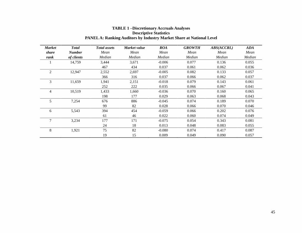
45

TABLE 1 –Discretionary Accruals Analyses

Descriptive Statistics

PANEL A: Ranking Auditors by Industry Market Share at National Level

Market Total Total assets Market value ROA GROWTH ABS(ACCRL) ADA

share Number Mean Mean Mean Mean Mean Mean

rank of clients Median Median Median Median Median Median

1 14,759 3,444 3,671 -0.006 0.077 0.136 0.055

467 434 0.037 0.061 0.062 0.036

2 12,947 2,552 2,697 -0.005 0.082 0.133 0.057

366 316 0.037 0.066 0.062 0.037

3 11,659 1,941 2,151 -0.018 0.079 0.143 0.061

252 222 0.035 0.066 0.067 0.041

4 10,519 1,433 1,660 -0.036 0.070 0.160 0.065

198 177 0.029 0.063 0.068 0.043

5 7,254 676 886 -0.045 0.074 0.189 0.070

99 82 0.028 0.066 0.070 0.046

6 5,543 394 454 -0.059 0.066 0.202 0.076

61 46 0.022 0.060 0.074 0.049

7 3,234 177 171 -0.075 0.054 0.343 0.081

24 18 0.013 0.048 0.083 0.055

8 1,921 75 82 -0.080 0.074 0.417 0.087

19 15 0.009 0.049 0.090 0.057

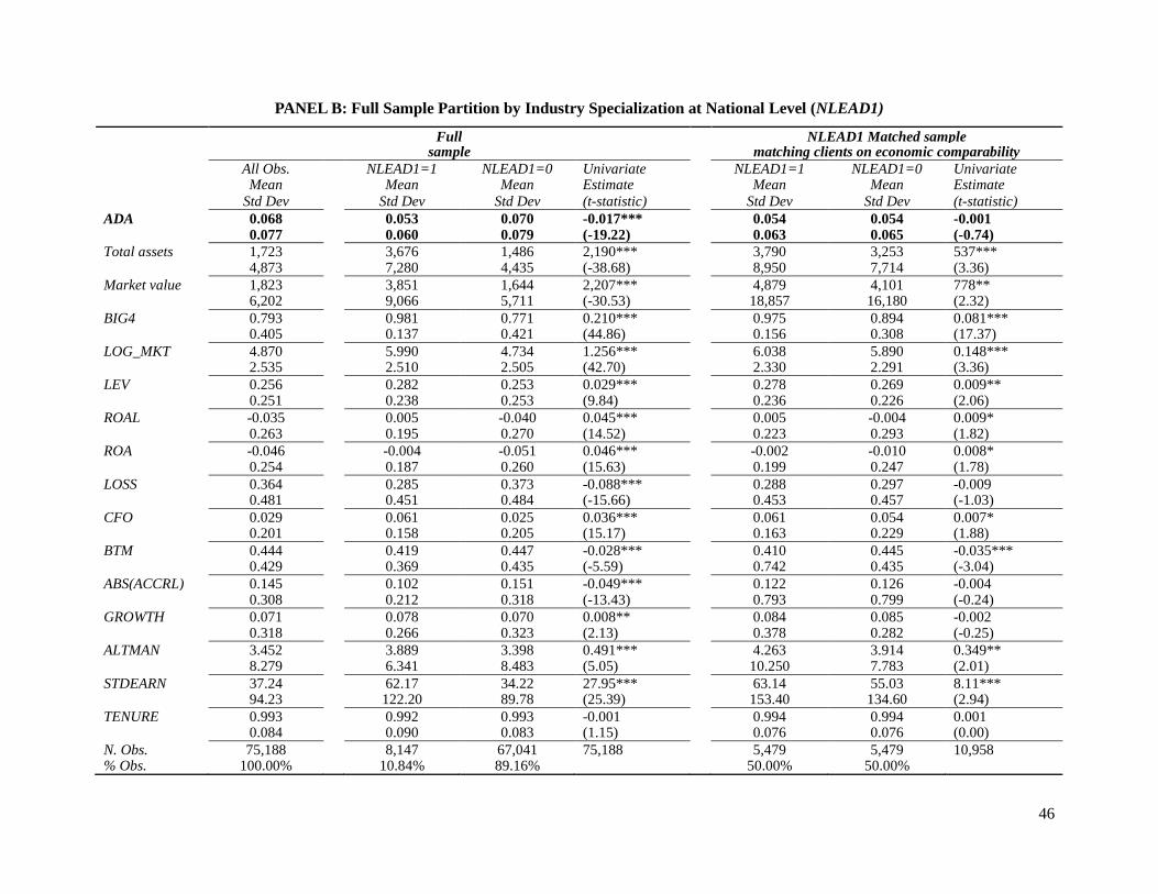
46

PANEL B: Full Sample Partition by Industry Specialization at National Level (NLEAD1)

Full NLEAD1 Matched sample sample matching clients on economic comparability

All Obs. NLEAD1=1 NLEAD1=0 Univariate NLEAD1=1 NLEAD1=0 Univariate Mean Mean Mean Estimate Mean Mean Estimate

Std Dev Std Dev Std Dev (t-statistic) Std Dev Std Dev (t-statistic)

ADA 0.068 0.053 0.070 -0.017*** 0.054 0.054 -0.001 0.077 0.060 0.079 (-19.22) 0.063 0.065 (-0.74)

Total assets 1,723 3,676 1,486 2,190*** 3,790 3,253 537*** 4,873 7,280 4,435 (-38.68) 8,950 7,714 (3.36)

Market value 1,823 3,851 1,644 2,207*** 4,879 4,101 778** 6,202 9,066 5,711 (-30.53) 18,857 16,180 (2.32)

BIG4 0.793 0.981 0.771 0.210*** 0.975 0.894 0.081*** 0.405 0.137 0.421 (44.86) 0.156 0.308 (17.37)

LOG_MKT 4.870 5.990 4.734 1.256*** 6.038 5.890 0.148*** 2.535 2.510 2.505 (42.70) 2.330 2.291 (3.36)

LEV 0.256 0.282 0.253 0.029*** 0.278 0.269 0.009** 0.251 0.238 0.253 (9.84) 0.236 0.226 (2.06)

ROAL -0.035 0.005 -0.040 0.045*** 0.005 -0.004 0.009* 0.263 0.195 0.270 (14.52) 0.223 0.293 (1.82)

ROA -0.046 -0.004 -0.051 0.046*** -0.002 -0.010 0.008* 0.254 0.187 0.260 (15.63) 0.199 0.247 (1.78)

LOSS 0.364 0.285 0.373 -0.088*** 0.288 0.297 -0.009 0.481 0.451 0.484 (-15.66) 0.453 0.457 (-1.03)

CFO 0.029 0.061 0.025 0.036*** 0.061 0.054 0.007* 0.201 0.158 0.205 (15.17) 0.163 0.229 (1.88)

BTM 0.444 0.419 0.447 -0.028*** 0.410 0.445 -0.035*** 0.429 0.369 0.435 (-5.59) 0.742 0.435 (-3.04)

ABS(ACCRL) 0.145 0.102 0.151 -0.049*** 0.122 0.126 -0.004 0.308 0.212 0.318 (-13.43) 0.793 0.799 (-0.24)

GROWTH 0.071 0.078 0.070 0.008** 0.084 0.085 -0.002 0.318 0.266 0.323 (2.13) 0.378 0.282 (-0.25)

ALTMAN 3.452 3.889 3.398 0.491*** 4.263 3.914 0.349** 8.279 6.341 8.483 (5.05) 10.250 7.783 (2.01)

STDEARN 37.24 62.17 34.22 27.95*** 63.14 55.03 8.11*** 94.23 122.20 89.78 (25.39) 153.40 134.60 (2.94)

TENURE 0.993 0.992 0.993 -0.001 0.994 0.994 0.001 0.084 0.090 0.083 (1.15) 0.076 0.076 (0.00)

N. Obs. 75,188 8,147 67,041 75,188 5,479 5,479 10,958 % Obs. 100.00% 10.84% 89.16% 50.00% 50.00%

47

PANEL C: Full Sample Partition by Industry Specialization at City Level (CLEAD1)

Full CLEAD1 Matched sample sample matching clients on economic comparability

All Obs. CLEAD1=1 CLEAD1=0 Univariate CLEAD1=1 CLEAD1=0 Univariate Mean Mean Mean Estimate Mean Mean Estimate

Std Dev Std Dev Std Dev (t-statistic) Std Dev Std Dev (t-statistic)

ADA 0.075 0.057 0.085 -0.028*** 0.056 0.059 -0.002* 0.089 0.070 0.097 (-22.68) 0.070 0.072 (-1.74)

Total assets 1,979 4,128 877 3,251*** 3,380 2,673 707*** 5,621 8,238 3,072 (33.44) 8,108 6,203 (4.89)

Market value 2,175 4,399 1,035 3,364*** 3,799 2,892 907*** 7,127 10,450 4,129 (35.01) 15,671 12,132 (3.23)

BIG4 0.718 0.940 0.605 0.335*** 0.963 0.855 0.108*** 0.450 0.239 0.489 (57.43) 0.189 0.352 (19.09)

LOG_MKT 5.164 6.367 4.548 1.819*** 6.407 6.228 0.179*** 2.522 2.382 2.365 (55.43) 1.969 1.922 (4.58)

LEV 0.242 0.259 0.233 0.025*** 0.249 0.238 0.011** 0.284 0.247 0.300 (6.45) 0.245 0.249 (2.17)

ROAL -0.079 -0.014 -0.112 0.098*** -0.014 -0.038 0.024*** 0.342 0.239 0.380 (20.98) 0.237 0.279 (4.65)

ROA -0.088 -0.022 -0.123 0.101*** -0.022 -0.042 0.020*** 0.321 0.223 0.356 (23.04) 0.221 0.244 (4.25)

LOSS 0.425 0.318 0.480 -0.162*** 0.319 0.364 -0.044*** 0.494 0.466 0.500 (-23.98) 0.466 0.481 (4.67)

CFO 0.003 0.053 -0.022 0.075*** 0.051 0.033 0.017*** 0.255 0.182 0.282 (21.58) 0.191 0.204 (4.40)

BTM 0.417 0.388 0.432 -0.044*** 0.409 0.425 -0.016** 0.461 0.380 0.498 (-7.01) 0.394 0.383 (2.06)

ABS(ACCRL) 0.125 0.092 0.142 -0.050*** 0.086 0.089 -0.003 0.171 0.118 0.191 (-21.21) 0.102 0.109 (1.34)

GROWTH 0.052 0.067 0.045 0.022*** 0.070 0.063 0.008 0.310 0.245 0.338 (5.04) 0.351 0.307 (1.19)

ALTMAN 2.306 3.630 1.627 2.003*** 4.433 3.968 0.465* 11.550 7.623 13.060 (12.57) 15.260 9.347 (1.83)

STDEARN 51.42 88.53 32.40 56.13*** 71.68 64.13 7.55*** 123.10 165.20 88.66 (33.75) 165.40 140.30 (2.46)

TENURE 0.997 0.996 0.998 -0.002*** 0.997 0.999 -0.002* 0.055 0.064 0.050 (-2.09) 0.053 0.035 (1.79)

N. Obs.a 23,307 7,897 15,410 23,307 4,979 4,979 9,958

% Obs. 100.00% 33.88% 66.12% 50.00% 50.00%

48

This table presents the descriptive statistics of the data used in the discretionary accruals analyses: Panel A shows descriptive statistics ranking the top eight auditors

by market share at industry-national level; Panel B shows descriptive statistics for the full sample and for a partition by industry specialization at national level

(NLEAD1); and Panel C shows descriptive statistics for the full sample and for a partition by industry specialization at city level (CLEAD1). Matching on economic

comparability refers to a pair-wise match of specialist and non-specialist auditors’ clients, based on industry, size, and returns covariance. Variable definitions are

included in Appendix A. *, **, *** indicate significance at the 0.10, 0.05 and 0.01 levels, respectively, using two-tailed tests. a The sample size is reduced to those

years with auditor city data in audit analytics matched to the U.S. Census Bureau 2003 list of Metropolitan Statistical Areas.

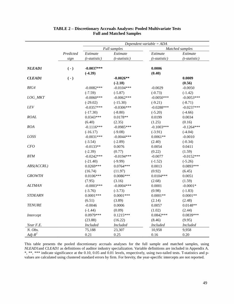
49

TABLE 2 – Discretionary Accruals Analyses: Pooled Multivariate Tests

Full and Matched Samples

Dependent variable = ADA

Full samples Matched samples

Predicted Estimate Estimate Estimate Estimate

sign (t-statistic) (t-statistic) (t-statistic) (t-statistic)

NLEAD1 ( - ) -0.0037*** 0.0006

(-4.39) (0.40)

CLEAD1 ( - ) -0.0026** 0.0009

(-2.18) (0.56)

BIG4 -0.0082*** -0.0104*** -0.0029 -0.0050

(-7.59) (-5.87) (-0.73) (-1.42)

LOG_MKT -0.0060*** -0.0062*** -0.0050*** -0.0053***

(-29.02) (-15.30) (-9.21) (-8.71)

LEV -0.0357*** -0.0306*** -0.0288*** -0.0237***

(-17.30) (-8.80) (-5.20) (-4.66)

ROAL 0.0343*** 0.0178** 0.0199 0.0034

(6.40) (2.35) (1.25) (0.16)

ROA -0.1116*** -0.0985*** -0.1003*** -0.1264***

(-16.17) (-9.08) (-3.91) (-4.04)

LOSS -0.0031*** -0.0044*** 0.0061** -0.0010

(-3.54) (-2.89) (2.40) (-0.34)

CFO -0.0133** 0.0076 0.0054 0.0411

(-2.39) (0.77) (0.22) (1.59)

BTM -0.0242*** -0.0194*** -0.0077 -0.0152***

(-21.40) (-9.99) (-1.52) (-5.26)

ABS(ACCRL) 0.0269*** 0.0764*** 0.0013 0.0893***

(16.74) (11.97) (0.92) (6.45)

GROWTH 0.0106*** 0.0086*** 0.0104*** 0.0051

(7.95) (3.16) (2.68) (1.59)

ALTMAN -0.0003*** -0.0004*** 0.0001 -0.0001*

(-3.76) (-3.73) (0.98) (-1.83)

STDEARN 0.0001*** 0.0001*** 0.0001** 0.0001**

(6.51) (3.89) (2.14) (2.48)

TENURE -0.0046 0.0006 0.0057 0.0148**

(-1.44) (0.09) (1.02) (2.44)

Intercept 0.0979*** 0.1215*** 0.0842*** 0.0839***

(23.88) (16.22) (8.46) (9.95)

Year F.E. Included Included Included Included

N. Obs. 75,188 23,307 10,958 9,958

Adj-R2 0.21 0.25 0.16 0.20

This table presents the pooled discretionary accruals analyses for the full sample and matched samples, using

NLEAD1and CLEAD1 as definitions of auditor industry specialization. Variable definitions are included in Appendix A.

*, **, *** indicate significance at the 0.10, 0.05 and 0.01 levels, respectively, using two-tailed tests. T-statistics and p-

values are calculated using clustered standard errors by firm. For brevity, the year-specific intercepts are not reported.

50

TABLE 3 – Discretionary Accruals Analyses: Multivariate Pair-Wise Differences Tests

Matched Samples

Dependent variable = ADAij

NLEAD1 CLEAD1

Predicted Estimate Estimate

sign (t-statistic) (t-statistic)

BIG4ij -0.0008 -0.0001

(-0.19) (-0.03)

LOG_MKTij 0.0052*** 0.0008

(3.68) (0.51)

LEVij 0.0003 -0.0021

(0.07) (-0.28)

ROALij 0.0148 0.0094

(1.12) (0.51)

ROAij -0.0901*** -0.1189***

(-3.92) (-3.84)

LOSSij 0.0033 -0.0021

(1.23) (-0.64)

CFOij 0.0210 0.0506*

(1.03) (1.75)

BTMij -0.0034 -0.0082*

(-1.34) (-1.90)

ABS(ACCRL)ij 0.0009 0.0659***

(0.19) (3.92)

GROWTHij 0.0075** -0.0011

(2.24) (-0.32)

ALTMANij -0.0003** -0.0003*

(-2.14) (-1.87)

STDEARNij 0.0001* 0.0001***

(1.73) (3.07)

TENUREij 0.0068 0.0199*

(0.77) (1.81)

Intercept ( - ) -0.0013 -0.0014

(-1.12) (-1.02)

Year F.E. Included Included

N. Obs. 5,479 4,979

Adj-R2 0.05 0.08

This table presents the pair-wise differences in discretionary accruals for the matched samples, using NLEAD1 and

CLEAD1 as definitions of auditor industry specialization. Variable definitions are included in Appendix A and ij

denotes the pair-wise difference between matched observations. *, **, *** indicate significance at the 0.10, 0.05 and

0.01 levels, respectively, using two-tailed tests. T-statistics and p-values are calculated using clustered standard

errors by firm. For brevity, the year-specific intercepts are not reported.

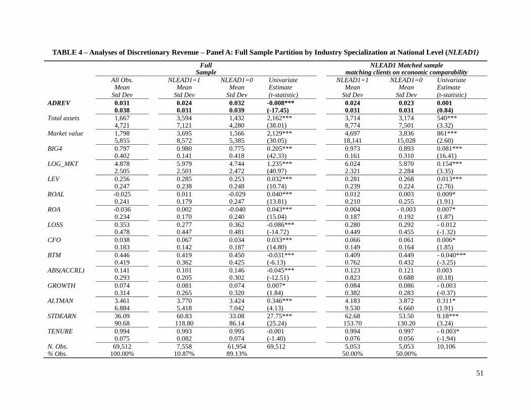
51

TABLE 4 – Analyses of Discretionary Revenue – Panel A: Full Sample Partition by Industry Specialization at National Level (NLEAD1)

Full NLEAD1 Matched sample Sample matching clients on economic comparability

All Obs. NLEAD1=1 NLEAD1=0 Univariate NLEAD1=1 NLEAD1=0 Univariate Mean Mean Mean Estimate Mean Mean Estimate Std Dev Std Dev Std Dev (t-statistic) Std Dev Std Dev (t-statistic)

ADREV 0.031 0.024 0.032 -0.008*** 0.024 0.023 0.001 0.038 0.031 0.039 (-17.45) 0.031 0.031 (0.84)

Total assets 1,667 3,594 1,432 2,162*** 3,714 3,174 540*** 4,721 7,121 4,280 (38.01) 8,774 7,501 (3.32)

Market value 1,798 3,695 1,566 2,129*** 4,697 3,836 861*** 5,855 8,572 5,385 (30.05) 18,141 15,028 (2.60)

BIG4 0.797 0.980 0.775 0.205*** 0.973 0.893 0.081*** 0.402 0.141 0.418 (42.33) 0.161 0.310 (16.41)

LOG_MKT 4.878 5.979 4.744 1.235*** 6.024 5.870 0.154*** 2.505 2.501 2.472 (40.97) 2.321 2.284 (3.35)

LEV 0.256 0.285 0.253 0.032*** 0.281 0.268 0.013*** 0.247 0.238 0.248 (10.74) 0.239 0.224 (2.76)

ROAL -0.025 0.011 -0.029 0.040*** 0.012 0.003 0.009* 0.241 0.179 0.247 (13.81) 0.210 0.255 (1.91)

ROA -0.036 0.002 -0.040 0.043*** 0.004 - 0.003 0.007* 0.234 0.170 0.240 (15.04) 0.187 0.192 (1.87)

LOSS 0.353 0.277 0.362 -0.086*** 0.280 0.292 - 0.012 0.478 0.447 0.481 (-14.72) 0.449 0.455 (-1.32)

CFO 0.038 0.067 0.034 0.033*** 0.066 0.061 0.006* 0.183 0.142 0.187 (14.80) 0.149 0.164 (1.85)

BTM 0.446 0.419 0.450 -0.031*** 0.409 0.449 - 0.040*** 0.419 0.362 0.425 (-6.13) 0.762 0.432 (-3.25)

ABS(ACCRL) 0.141 0.101 0.146 -0.045*** 0.123 0.121 0.003 0.293 0.205 0.302 (-12.51) 0.823 0.688 (0.18)

GROWTH 0.074 0.081 0.074 0.007* 0.084 0.086 - 0.003 0.314 0.265 0.320 (1.84) 0.382 0.283 (-0.37)

ALTMAN 3.461 3.770 3.424 0.346*** 4.183 3.872 0.311* 6.884 5.418 7.042 (4.13) 9.530 6.660 (1.91)

STDEARN 36.09 60.83 33.08 27.75*** 62.68 53.50 9.18*** 90.68 118.80 86.14 (25.24) 153.70 130.20 (3.24)

TENURE 0.994 0.993 0.995 -0.001 0.994 0.997 - 0.003* 0.075 0.082 0.074 (-1.40) 0.076 0.056 (-1.94)

N. Obs. 69,512 7,558 61,954 69,512 5,053 5,053 10,106 % Obs. 100.00% 10.87% 89.13% 50.00% 50.00%

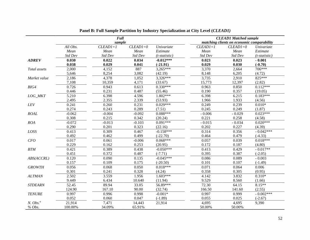
52

Panel B: Full Sample Partition by Industry Specialization at City Level (CLEAD1)

Full CLEAD1 Matched sample sample matching clients on economic comparability

All Obs. CLEAD1=1 CLEAD1=0 Univariate CLEAD1=1 CLEAD1=0 Univariate Mean Mean Mean Estimate Mean Mean Estimate Std Dev Std Dev Std Dev (t-statistic) Std Dev Std Dev (t-statistic)

ADREV 0.030 0.022 0.034 -0.012*** 0.023 0.023 - 0.001 0.038 0.029 0.041 (-21.91) 0.029 0.030 (-0.70)

Total assets 2,000 4,152 887 3,265*** 3,370 2,664 706*** 5,646 8,254 3,082 (42.19) 8,148 6,205 (4.72)

Market value 2,186 4,378 1,052 3,326*** 3,735 2,910 825*** 7,108 10,359 4,171 (33.67) 15,773 12,397 (2.82)

BIG4 0.726 0.943 0.613 0.330*** 0.963 0.850 0.112*** 0.446 0.231 0.487 (55.46) 0.190 0.357 (19.05)

LOG_MKT 5.210 6.398 4.596 1.802*** 6.398 6.215 0.183*** 2.495 2.355 2.339 (53.93) 1.966 1.933 (4.56)

LEV 0.241 0.260 0.231 0.029*** 0.249 0.239 0.010* 0.274 0.243 0.289 (7.51) 0.245 0.249 (1.87)

ROAL -0.062 -0.004 -0.092 0.088*** - 0.006 - 0.029 0.023*** 0.308 0.215 0.342 (20.24) 0.221 0.258 (4.58)

ROA -0.072 -0.013 -0.103 0.091*** - 0.015 - 0.034 0.020*** 0.290 0.201 0.323 (22.16) 0.202 0.227 (4.39)

LOSS 0.413 0.309 0.467 -0.158*** 0.314 0.356 - 0.042*** 0.492 0.462 0.499 (-22.70) 0.464 0.479 (-4.33)

CFO 0.017 0.061 -0.006 0.068*** 0.057 0.039 0.018*** 0.229 0.162 0.253 (20.95) 0.172 0.187 (4.80)

BTM 0.421 0.389 0.438 -0.050*** 0.413 0.429 - 0.017** 0.451 0.372 0.487 (-7.71) 0.395 0.387 (-2.05)

ABS(ACCRL) 0.120 0.090 0.135 -0.045*** 0.086 0.089 - 0.003 0.157 0.109 0.175 (-20.50) 0.101 0.107 (-1.49)

GROWTH 0.056 0.068 0.050 0.018*** 0.071 0.064 0.006 0.301 0.241 0.328 (4.24) 0.358 0.305 (0.95)

ALTMAN 2.502 3.559 1.956 1.603*** 4.142 3.832 0.310* 9.449 6.434 10.640 (11.94) 9.529 8.560 (1.66)

STDEARN 52.45 89.94 33.05 56.89*** 72.30 64.15 8.15** 124.90 167.10 90.00 (32.74) 166.50 141.60 (2.55)

TENURE 0.997 0.996 0.998 -0.001* 0.997 0.999 - 0.002*** 0.052 0.060 0.047 (-1.89) 0.055 0.025 (-2.67)

N. Obs.a 21,914 7,471 14,443 21,914 4,695 4,695 9,390

% Obs. 100.00% 34.09% 65.91% 50.00% 50.00%

53

This table presents the descriptive statistics of the data used in the discretionary revenue analyses: Panel A shows descriptive statistics for the full sample and for a

partition by industry specialization at national level (NLEAD1); and, Panel B shows descriptive statistics for the full sample and for a partition by industry

specialization at city level (CLEAD1). Matching on economic comparability refers to a pair-wise match of specialist and non-specialist auditors’ clients, based on

industry, size, and returns covariance. Variable definitions are included in Appendix A. *, **, *** indicate significance at the 0.10, 0.05 and 0.01 levels, respectively,

using two-tailed tests. a

The sample size is reduced to those years with auditor city data in audit analytics matched to the U.S. Census Bureau 2003 list of

Metropolitan Statistical Areas.

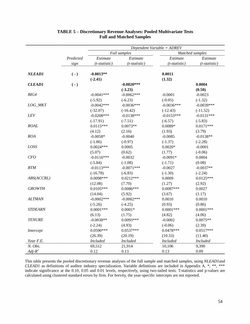
54

TABLE 5 – Discretionary Revenue Analyses: Pooled Multivariate Tests

Full and Matched Samples

Dependent Variable = ADREV

Full samples Matched samples

Predicted Estimate Estimate Estimate Estimate

sign (t-statistic) (t-statistic) (t-statistic) (t-statistic)

NLEAD1 ( - ) -0.0013** 0.0011

(-2.41) (1.32)

CLEAD1 ( - ) -0.0020*** 0.0004

(-3.23) (0.50)

BIG4 -0.0041*** -0.0062*** -0.0001 -0.0023

(-5.92) (-6.23) (-0.05) (-1.32)

LOG_MKT -0.0042*** -0.0036*** -0.0036*** -0.0039***

(-32.07) (-16.42) (-12.43) (-11.52)

LEV -0.0208*** -0.0138*** -0.0153*** -0.0131***

(-17.91) (-7.51) (-6.57) (-5.83)

ROAL 0.0115*** 0.0073** 0.0089* 0.0171***

(4.12) (2.16) (1.93) (3.79)

ROA -0.0058* -0.0040 -0.0085 -0.0138**

(-1.86) (-0.97) (-1.37) (-2.28)

LOSS 0.0024*** 0.0005 0.0020* -0.0001

(5.07) (0.62) (1.77) (-0.06)

CFO -0.0116*** -0.0032 -0.0091* 0.0004

(-5.84) (-1.08) (-1.71) (0.08)

BTM -0.0113*** -0.0071*** -0.0027 -0.0037**

(-16.78) (-6.83) (-1.30) (-2.24)

ABS(ACCRL) 0.0098*** 0.0212*** 0.0009 0.0125***

(12.08) (7.70) (1.27) (2.92)

GROWTH 0.0105*** 0.0086*** 0.0087*** 0.0027

(14.04) (5.92) (3.67) (1.17)

ALTMAN -0.0002*** -0.0002*** 0.0010 0.0010

(-5.26) (-4.25) (0.93) (0.86)

STDEARN 0.0001*** 0.0001* 0.0001*** 0.0001***

(6.13) (1.75) (4.82) (4.06)

TENURE -0.0038** 0.0093*** -0.0002 0.0075**

(-2.24) (4.93) (-0.06) (2.39)

Intercept 0.0590*** 0.0537*** 0.0478*** 0.0517***

(26.39) (20.19) (10.33) (11.40)

Year F.E. Included Included Included Included

N. Obs. 69,512 21,914 10,106 9,390

Adj-R2 0.12 0.13 0.13 0.09

This table presents the pooled discretionary revenue analyses of the full sample and matched samples, using NLEAD1and

CLEAD1 as definitions of auditor industry specialization. Variable definitions are included in Appendix A. *, **, ***

indicate significance at the 0.10, 0.05 and 0.01 levels, respectively, using two-tailed tests. T-statistics and p-values are

calculated using clustered standard errors by firm. For brevity, the year-specific intercepts are not reported.

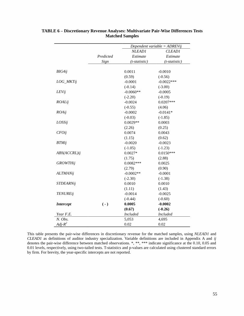
55

TABLE 6 – Discretionary Revenue Analyses: Multivariate Pair-Wise Differences Tests

Matched Samples

Dependent variable = ADREVij

NLEAD1 CLEAD1

Predicted Estimate Estimate

Sign (t-statistic) (t-statistic)

BIG4ij 0.0011 -0.0010

(0.59) (-0.56)

LOG_MKTij -0.0001 -0.0022***

(-0.14) (-3.00)

LEVij -0.0060** -0.0005

(-2.20) (-0.19)

ROALij -0.0024 0.0207***

(-0.55) (4.06)

ROAij -0.0002 -0.0141*

(-0.03) (-1.85)

LOSSij 0.0029** 0.0003

(2.26) (0.25)

CFOij 0.0074 0.0043

(1.15) (0.62)

BTMij -0.0020 -0.0023

(-1.05) (-1.23)

ABS(ACCRL)ij 0.0027* 0.0150***

(1.75) (2.88)

GROWTHij 0.0082*** 0.0025

(2.79) (0.90)

ALTMANij -0.0002** -0.0001

(-2.30) (-1.38)

STDEARNij 0.0010 0.0010

(1.11) (1.43)

TENUREij -0.0014 -0.0025

(-0.44) (-0.60)

Intercept ( - ) 0.0005 -0.0002

(0.67) (-0.26)

Year F.E. Included Included

N. Obs. 5,053 4,695

Adj-R2 0.02 0.02

This table presents the pair-wise differences in discretionary revenue for the matched samples, using NLEAD1 and

CLEAD1 as definitions of auditor industry specialization. Variable definitions are included in Appendix A and ij

denotes the pair-wise difference between matched observations. *, **, *** indicate significance at the 0.10, 0.05 and

0.01 levels, respectively, using two-tailed tests. T-statistics and p-values are calculated using clustered standard errors

by firm. For brevity, the year-specific intercepts are not reported.

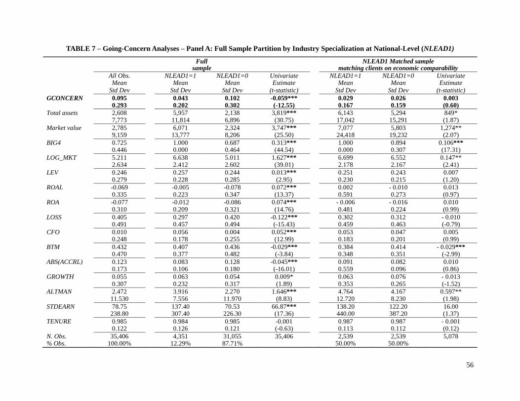
56

TABLE 7 – Going-Concern Analyses – Panel A: Full Sample Partition by Industry Specialization at National-Level (NLEAD1)

Full NLEAD1 Matched sample sample matching clients on economic comparability

All Obs. NLEAD1=1 NLEAD1=0 Univariate NLEAD1=1 NLEAD1=0 Univariate Mean Mean Mean Estimate Mean Mean Estimate

Std Dev Std Dev Std Dev (t-statistic) Std Dev Std Dev (t-statistic)

GCONCERN 0.095 0.043 0.102 -0.059*** 0.029 0.026 0.003 0.293 0.202 0.302 (-12.55) 0.167 0.159 (0.60)

Total assets 2,608 5,957 2,138 3,819*** 6,143 5,294 849* 7,773 11,814 6,896 (30.75) 17,042 15,291 (1.87)

Market value 2,785 6,071 2,324 3,747*** 7,077 5,803 1,274** 9,159 13,777 8,206 (25.50) 24,418 19,232 (2.07)

BIG4 0.725 1.000 0.687 0.313*** 1.000 0.894 0.106*** 0.446 0.000 0.464 (44.54) 0.000 0.307 (17.31)

LOG_MKT 5.211 6.638 5.011 1.627*** 6.699 6.552 0.147** 2.634 2.412 2.602 (39.01) 2.178 2.167 (2.41)

LEV 0.246 0.257 0.244 0.013*** 0.251 0.243 0.007 0.279 0.228 0.285 (2.95) 0.230 0.215 (1.20)

ROAL -0.069 -0.005 -0.078 0.072*** 0.002 - 0.010 0.013 0.335 0.223 0.347 (13.37) 0.591 0.273 (0.97)

ROA -0.077 -0.012 -0.086 0.074*** - 0.006 - 0.016 0.010 0.310 0.209 0.321 (14.76) 0.481 0.224 (0.99)

LOSS 0.405 0.297 0.420 -0.122*** 0.302 0.312 - 0.010 0.491 0.457 0.494 (-15.43) 0.459 0.463 (-0.79)

CFO 0.010 0.056 0.004 0.052*** 0.053 0.047 0.005 0.248 0.178 0.255 (12.99) 0.183 0.201 (0.99)

BTM 0.432 0.407 0.436 -0.029*** 0.384 0.414 - 0.029*** 0.470 0.377 0.482 (-3.84) 0.348 0.351 (-2.99)

ABS(ACCRL) 0.123 0.083 0.128 -0.045*** 0.091 0.082 0.010 0.173 0.106 0.180 (-16.01) 0.559 0.096 (0.86)

GROWTH 0.055 0.063 0.054 0.009* 0.063 0.076 - 0.013 0.307 0.232 0.317 (1.89) 0.353 0.265 (-1.52)

ALTMAN 2.472 3.916 2.270 1.646*** 4.764 4.167 0.597** 11.530 7.556 11.970 (8.83) 12.720 8.230 (1.98)

STDEARN 78.75 137.40 70.53 66.87*** 138.20 122.20 16.00 238.80 307.40 226.30 (17.36) 440.00 387.20 (1.37)

TENURE 0.985 0.984 0.985 -0.001 0.987 0.987 - 0.001 0.122 0.126 0.121 (-0.63) 0.113 0.112 (0.12)

N. Obs. 35,406 4,351 31,055 35,406 2,539 2,539 5,078 % Obs. 100.00% 12.29% 87.71% 50.00% 50.00%

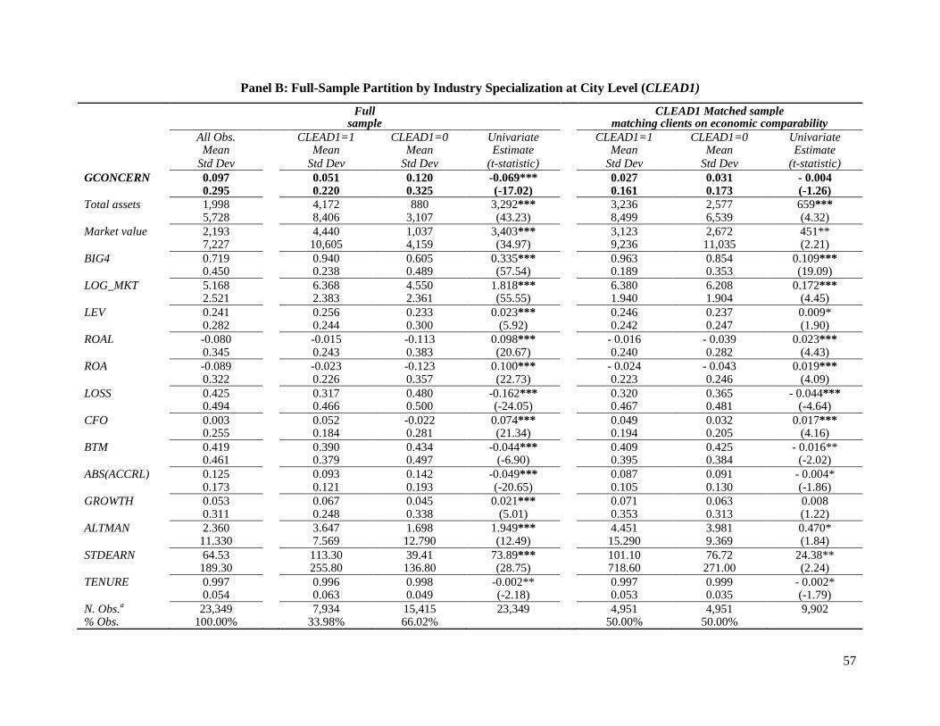
57

Panel B: Full-Sample Partition by Industry Specialization at City Level (CLEAD1)

Full CLEAD1 Matched sample sample matching clients on economic comparability

All Obs. CLEAD1=1 CLEAD1=0 Univariate CLEAD1=1 CLEAD1=0 Univariate Mean Mean Mean Estimate Mean Mean Estimate

Std Dev Std Dev Std Dev (t-statistic) Std Dev Std Dev (t-statistic)

GCONCERN 0.097 0.051 0.120 -0.069*** 0.027 0.031 - 0.004 0.295 0.220 0.325 (-17.02) 0.161 0.173 (-1.26)

Total assets 1,998 4,172 880 3,292*** 3,236 2,577 659*** 5,728 8,406 3,107 (43.23) 8,499 6,539 (4.32)

Market value 2,193 4,440 1,037 3,403*** 3,123 2,672 451** 7,227 10,605 4,159 (34.97) 9,236 11,035 (2.21)

BIG4 0.719 0.940 0.605 0.335*** 0.963 0.854 0.109*** 0.450 0.238 0.489 (57.54) 0.189 0.353 (19.09)

LOG_MKT 5.168 6.368 4.550 1.818*** 6.380 6.208 0.172*** 2.521 2.383 2.361 (55.55) 1.940 1.904 (4.45)

LEV 0.241 0.256 0.233 0.023*** 0.246 0.237 0.009* 0.282 0.244 0.300 (5.92) 0.242 0.247 (1.90)

ROAL -0.080 -0.015 -0.113 0.098*** - 0.016 - 0.039 0.023*** 0.345 0.243 0.383 (20.67) 0.240 0.282 (4.43)

ROA -0.089 -0.023 -0.123 0.100*** - 0.024 - 0.043 0.019*** 0.322 0.226 0.357 (22.73) 0.223 0.246 (4.09)

LOSS 0.425 0.317 0.480 -0.162*** 0.320 0.365 - 0.044*** 0.494 0.466 0.500 (-24.05) 0.467 0.481 (-4.64)

CFO 0.003 0.052 -0.022 0.074*** 0.049 0.032 0.017*** 0.255 0.184 0.281 (21.34) 0.194 0.205 (4.16)

BTM 0.419 0.390 0.434 -0.044*** 0.409 0.425 - 0.016** 0.461 0.379 0.497 (-6.90) 0.395 0.384 (-2.02)

ABS(ACCRL) 0.125 0.093 0.142 -0.049*** 0.087 0.091 - 0.004* 0.173 0.121 0.193 (-20.65) 0.105 0.130 (-1.86)

GROWTH 0.053 0.067 0.045 0.021*** 0.071 0.063 0.008 0.311 0.248 0.338 (5.01) 0.353 0.313 (1.22)

ALTMAN 2.360 3.647 1.698 1.949*** 4.451 3.981 0.470* 11.330 7.569 12.790 (12.49) 15.290 9.369 (1.84)

STDEARN 64.53 113.30 39.41 73.89***

*** 101.10 76.72 24.38**

189.30 255.80 136.80 (28.75) 718.60 271.00 (2.24)

TENURE 0.997 0.996 0.998 -0.002** 0.997 0.999 - 0.002* 0.054 0.063 0.049 (-2.18) 0.053 0.035 (-1.79)

N. Obs.a 23,349 7,934 15,415 23,349 4,951 4,951 9,902

% Obs. 100.00% 33.98% 66.02% 50.00% 50.00%

58

This table presents the descriptive statistics of the data used in the analysis of propensity to issue a going-concern opinion: Panel A shows descriptive statistics for

the full sample and for a partition by industry specialization at national level (NLEAD1); and Panel B shows descriptive statistics for the full sample and for a

partition by industry specialization at city level (CLEAD1). Matching on economic comparability refers to a pair-wise match of specialist and non-specialist

auditors’ clients, based on industry, size, and returns covariance. Variable definitions are included in Appendix A. *, **, *** indicate significance at the 0.10, 0.05

and 0.01 levels, respectively, using two-tailed tests. a The sample size is reduced to those years with auditor city data in audit analytics matched to the U.S. Census

Bureau 2003 list of Metropolitan Statistical Areas.

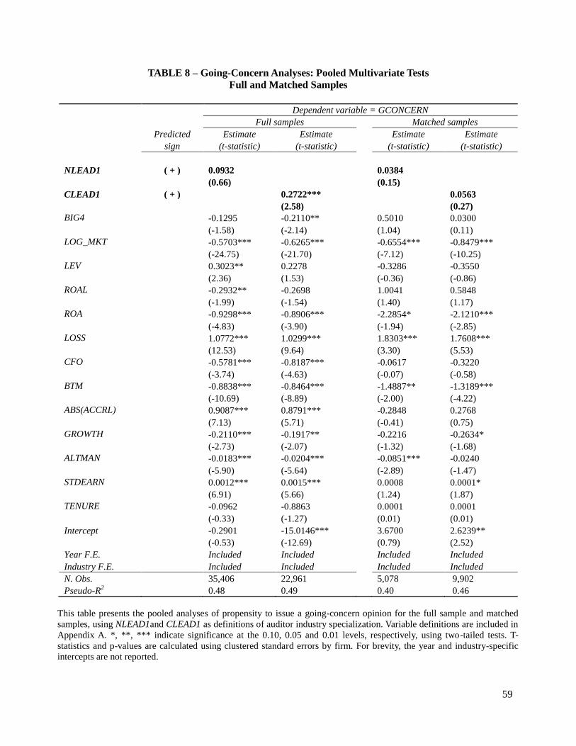
59

TABLE 8 – Going-Concern Analyses: Pooled Multivariate Tests

Full and Matched Samples

Dependent variable = GCONCERN

Full samples Matched samples

Predicted Estimate Estimate Estimate Estimate

sign (t-statistic) (t-statistic) (t-statistic) (t-statistic)

NLEAD1 ( + ) 0.0932 0.0384

(0.66) (0.15)

CLEAD1 ( + ) 0.2722*** 0.0563

(2.58) (0.27)

BIG4 -0.1295 -0.2110** 0.5010 0.0300

(-1.58) (-2.14) (1.04) (0.11)

LOG_MKT -0.5703*** -0.6265*** -0.6554*** -0.8479***

(-24.75) (-21.70) (-7.12) (-10.25)

LEV 0.3023** 0.2278 -0.3286 -0.3550

(2.36) (1.53) (-0.36) (-0.86)

ROAL -0.2932** -0.2698 1.0041 0.5848

(-1.99) (-1.54) (1.40) (1.17)

ROA -0.9298*** -0.8906*** -2.2854* -2.1210***

(-4.83) (-3.90) (-1.94) (-2.85)

LOSS 1.0772*** 1.0299*** 1.8303*** 1.7608***

(12.53) (9.64) (3.30) (5.53)

CFO -0.5781*** -0.8187*** -0.0617 -0.3220

(-3.74) (-4.63) (-0.07) (-0.58)

BTM -0.8838*** -0.8464*** -1.4887** -1.3189***

(-10.69) (-8.89) (-2.00) (-4.22)

ABS(ACCRL) 0.9087*** 0.8791*** -0.2848 0.2768

(7.13) (5.71) (-0.41) (0.75)

GROWTH -0.2110*** -0.1917** -0.2216 -0.2634*

(-2.73) (-2.07) (-1.32) (-1.68)

ALTMAN -0.0183*** -0.0204*** -0.0851*** -0.0240

(-5.90) (-5.64) (-2.89) (-1.47)

STDEARN 0.0012*** 0.0015*** 0.0008 0.0001*

(6.91) (5.66) (1.24) (1.87)

TENURE -0.0962 -0.8863 0.0001 0.0001

(-0.33) (-1.27) (0.01) (0.01)

Intercept -0.2901 -15.0146*** 3.6700 2.6239**

(-0.53) (-12.69) (0.79) (2.52)

Year F.E. Included Included Included Included

Industry F.E. Included Included Included Included

N. Obs. 35,406 22,961 5,078 9,902

Pseudo-R2 0.48 0.49 0.40 0.46

This table presents the pooled analyses of propensity to issue a going-concern opinion for the full sample and matched

samples, using NLEAD1and CLEAD1 as definitions of auditor industry specialization. Variable definitions are included in

Appendix A. *, **, *** indicate significance at the 0.10, 0.05 and 0.01 levels, respectively, using two-tailed tests. T-

statistics and p-values are calculated using clustered standard errors by firm. For brevity, the year and industry-specific

intercepts are not reported.

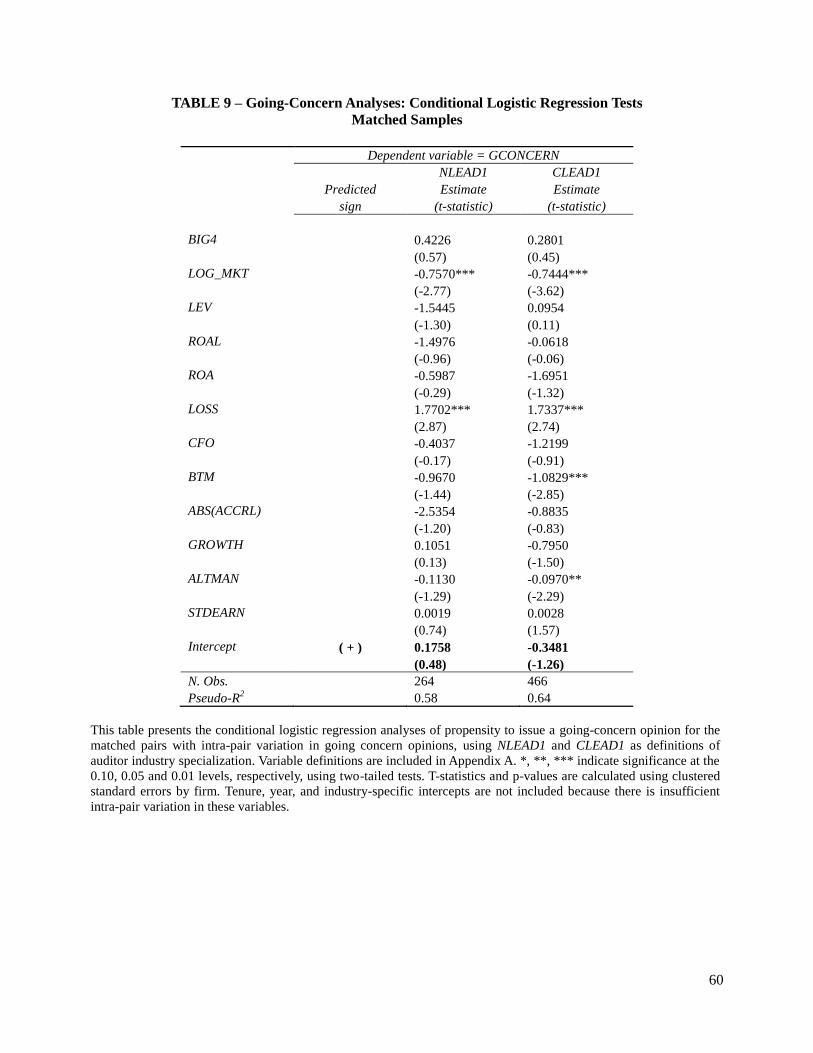
60

TABLE 9 – Going-Concern Analyses: Conditional Logistic Regression Tests

Matched Samples

Dependent variable = GCONCERN

NLEAD1 CLEAD1

Predicted Estimate Estimate

sign (t-statistic) (t-statistic)

BIG4 0.4226 0.2801

(0.57) (0.45)

LOG_MKT -0.7570*** -0.7444***

(-2.77) (-3.62)

LEV -1.5445 0.0954

(-1.30) (0.11)

ROAL -1.4976 -0.0618

(-0.96) (-0.06)

ROA -0.5987 -1.6951

(-0.29) (-1.32)

LOSS 1.7702*** 1.7337***

(2.87) (2.74)

CFO -0.4037 -1.2199

(-0.17) (-0.91)

BTM -0.9670 -1.0829***

(-1.44) (-2.85)

ABS(ACCRL) -2.5354 -0.8835

(-1.20) (-0.83)

GROWTH 0.1051 -0.7950

(0.13) (-1.50)

ALTMAN -0.1130 -0.0970**

(-1.29) (-2.29)

STDEARN 0.0019 0.0028

(0.74) (1.57)

Intercept ( + ) 0.1758 -0.3481

(0.48) (-1.26)

N. Obs. 264 466

Pseudo-R2 0.58 0.64

This table presents the conditional logistic regression analyses of propensity to issue a going-concern opinion for the

matched pairs with intra-pair variation in going concern opinions, using NLEAD1 and CLEAD1 as definitions of

auditor industry specialization. Variable definitions are included in Appendix A. *, **, *** indicate significance at the

0.10, 0.05 and 0.01 levels, respectively, using two-tailed tests. T-statistics and p-values are calculated using clustered

standard errors by firm. Tenure, year, and industry-specific intercepts are not included because there is insufficient

intra-pair variation in these variables.

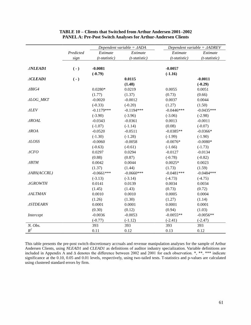
61

TABLE 10 – Clients that Switched from Arthur Andersen 2001–2002

PANEL A: Pre-Post Switch Analyses for Arthur-Andersen Clients

Dependent variable = ΔADA Dependent variable = ΔADREV

Predicted Estimate Estimate Estimate Estimate

sign (t-statistic) (t-statistic) (t-statistic) (t-statistic)

ΔNLEAD1 ( - ) -0.0081 -0.0057

(-0.79) (-1.16)

ΔCLEAD1 ( - ) 0.0115 -0.0011

(1.48) (-0.29)

ΔBIG4 0.0280* 0.0219 0.0055 0.0051

(1.77) (1.37) (0.73) (0.66)

ΔLOG_MKT -0.0020 -0.0012 0.0037 0.0044

(-0.33) (-0.20) (1.27) (1.50)

ΔLEV -0.1179*** -0.1194*** -0.0446*** -0.0435***

(-3.90) (-3.96) (-3.06) (-2.98)

ΔROAL -0.0343 -0.0361 0.0013 -0.0011

(-1.07) (-1.14) (0.08) (-0.07)

ΔROA -0.0520 -0.0511 -0.0385** -0.0366*

(-1.30) (-1.28) (-1.99) (-1.90)

ΔLOSS -0.0060 -0.0058 -0.0076* -0.0080*

(-0.63) (-0.61) (-1.66) (-1.73)

ΔCFO 0.0297 0.0294 -0.0127 -0.0134

(0.88) (0.87) (-0.78) (-0.82)

ΔBTM 0.0042 0.0044 0.0025* 0.0023

(1.37) (1.44) (1.73) (1.59)

ΔABS(ACCRL) -0.0661*** -0.0660*** -0.0481*** -0.0484***

(-3.13) (-3.14) (-4.73) (-4.75)

ΔGROWTH 0.0141 0.0139 0.0034 0.0034

(1.45) (1.43) (0.73) (0.72)

ΔALTMAN 0.0010 0.0010 0.0005 0.0004

(1.26) (1.30) (1.27) (1.14)

ΔSTDEARN 0.0001 0.0001 0.0001 0.0001

(0.30) (0.12) (0.94) (1.03)

Intercept -0.0036 -0.0053 -0.0055** -0.0056**

(-0.77) (-1.12) (-2.41) (-2.47)

N. Obs. 393 393 393 393

R2 0.11 0.12 0.13 0.12

This table presents the pre-post switch discretionary accruals and revenue manipulation analyses for the sample of Arthur

Andersen Clients, using NLEAD1 and CLEAD1 as definitions of auditor industry specialization. Variable definitions are

included in Appendix A and Δ denotes the difference between 2002 and 2001 for each observation. *, **, *** indicate

significance at the 0.10, 0.05 and 0.01 levels, respectively, using two-tailed tests. T-statistics and p-values are calculated

using clustered standard errors by firm.

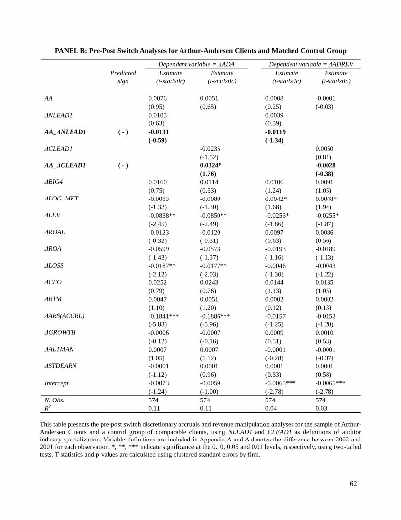
62

PANEL B: Pre-Post Switch Analyses for Arthur-Andersen Clients and Matched Control Group

Dependent variable = ΔADA Dependent variable = ΔADREV

Predicted Estimate Estimate Estimate Estimate

sign (t-statistic) (t-statistic) (t-statistic) (t-statistic)

AA 0.0076 0.0051 0.0008 -0.0001

(0.95) (0.65) (0.25) (-0.03)

ΔNLEAD1 0.0105 0.0039

(0.63) (0.59)

AA_ΔNLEAD1 ( - ) -0.0131 -0.0119

(-0.59) (-1.34)

ΔCLEAD1 -0.0235 0.0050

(-1.52) (0.81)

AA_ΔCLEAD1 ( - ) 0.0324* -0.0028

(1.76) (-0.38)

ΔBIG4 0.0160 0.0114 0.0106 0.0091

(0.75) (0.53) (1.24) (1.05)

ΔLOG_MKT -0.0083 -0.0080 0.0042* 0.0048*

(-1.32) (-1.30) (1.68) (1.94)

ΔLEV -0.0838** -0.0850** -0.0253* -0.0255*

(-2.45) (-2.49) (-1.86) (-1.87)

ΔROAL -0.0123 -0.0120 0.0097 0.0086

(-0.32) (-0.31) (0.63) (0.56)

ΔROA -0.0599 -0.0573 -0.0193 -0.0189

(-1.43) (-1.37) (-1.16) (-1.13)

ΔLOSS -0.0187** -0.0177** -0.0046 -0.0043

(-2.12) (-2.03) (-1.30) (-1.22)

ΔCFO 0.0252 0.0243 0.0144 0.0135

(0.79) (0.76) (1.13) (1.05)

ΔBTM 0.0047 0.0051 0.0002 0.0002

(1.10) (1.20) (0.12) (0.13)

ΔABS(ACCRL) -0.1841*** -0.1886*** -0.0157 -0.0152

(-5.83) (-5.96) (-1.25) (-1.20)

ΔGROWTH -0.0006 -0.0007 0.0009 0.0010

(-0.12) (-0.16) (0.51) (0.53)

ΔALTMAN 0.0007 0.0007 -0.0001 -0.0001

(1.05) (1.12) (-0.28) (-0.37)

ΔSTDEARN -0.0001 0.0001 0.0001 0.0001

(-1.12) (0.96) (0.33) (0.58)

Intercept -0.0073 -0.0059 -0.0065*** -0.0065***

(-1.24) (-1.00) (-2.78) (-2.78)

N. Obs. 574 574 574 574

R2 0.11 0.11 0.04 0.03

This table presents the pre-post switch discretionary accruals and revenue manipulation analyses for the sample of Arthur-

Andersen Clients and a control group of comparable clients, using NLEAD1 and CLEAD1 as definitions of auditor

industry specialization. Variable definitions are included in Appendix A and Δ denotes the difference between 2002 and

2001 for each observation. *, **, *** indicate significance at the 0.10, 0.05 and 0.01 levels, respectively, using two-tailed

tests. T-statistics and p-values are calculated using clustered standard errors by firm.

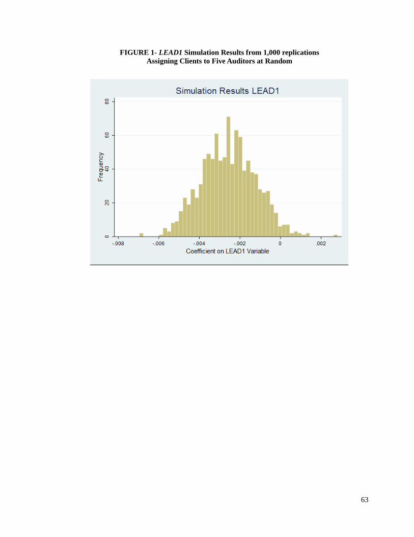
63

FIGURE 1- LEAD1 Simulation Results from 1,000 replications

Assigning Clients to Five Auditors at Random