Does Bureaucratic Ownership Lead to

Better Service Delivery in Social Projects?

Research Proposal

Jonathan Phillips

12th December 2012

1 Summary

Background: Nigeria’s debt-relief fund made an exogenous pot of funds available for the construction of

education/health/water projects. All of these projects are managed and maintained by the local government.

However, for the selection of initial project location the pot was split in two between (i) local governments

and (ii) legislators.

Treatment: There is ‘bureaucratic ownership’ of a project where its location is selected by the local

government (‘CGS’ projects) instead of the legislator for the locality (‘QW’ projects). The control condition

is where the legislator selects project location and there is no bureaucratic ownership.

Outcome: Performance of the project in terms of service delivery outputs. Multiple measures are

available, eg. availability of equipment, number of staff, availability of electricity, etc.

Theory: Ownership may have a positive impact on project service delivery performance where the

bureaucrat is able to claim credit and private rewards only for projects they themselves have initiated, creating

an incentive to exert more effort in maintenance. On the other hand, location selection by a legislator enables

new accountability mechanisms that may also induce greater bureaucratic effort in maintenance. The effect

of ownership on service delivery is therefore ambiguous and an important area for empirical study.

Identification Strategy: Two exogenous pots of funds are available for project selection by bureaucrats

and legislators respectively. Under certain assumptions, each pot provides a feasible counterfactual for the

other for circumstances in which both types of actor make some project location choices.

1

A total ‘bureaucratic ownership’ effect is straightforward to estimate as the difference in means between

CGS and QW projects. However, treatment by changing the identity of the decision-maker to a bureaucrat

inherently means changing a bundle of attributes beyond just the simple congruence between project selector

and project operator. Since bureaucrats may have systematically different information on project potential,

and systematically different political affiliations, bureaucratic ownership has multiple effects. To isolate the

aspects of ownership described in the theory section, I control for a host of spatial variables that might affect

location decisions.

2 Introduction and Motivation

The role of bureaucrats in developing countries is often characterized as rent-seeking agents with no inde-

pendent capacity or outcome-oriented motivations. Yet, despite the obvious challenges, thousands of schools

and clinics operate every day and a complex network of supplies, payments and maintenance contracts is

overseen by local bureaucrats.

Most striking is the local variation in service delivery quality. Anecdotal stories of neighbouring schools

operating at very different levels of performance abound. In Nigeria, variation in primary school completion

rates ranges from 2% to 99% ( Federal Government of Nigeria, 2010b ). Access to an improved water source

in Local Governments ranges from a reported 0% to 100% ( Federal Government of Nigeria, 2006 ).

While there are a range of possible explanations for this local variation, I focus on one aspect: The

‘ownership’ of a project by the bureaucracy. I characterize ‘ownership’ as the participation of the bureaucracy

in selecting a project and its location. Lack of ownership is a common complaint among bureaucrats. For

example, an extensive survey of Nigerian civil servants concluded that “Many civil servants feel that they

have increasingly been marginalised from undertaking their own duties...[and] are no longer engaged with

the process of planning and implementation”(Federal Government of Nigeria, 2011 ).

Participation of the bureaucracy in project selection and location is a move towards potentially less

politicized decision-making. But it may also lead to less representative and less accountable decision-making.

Understanding whether bureaucratic participation and ownership is a positive force that can improve

service delivery, or a negative force, is crucial to understanding how bureaucratic politics works. It is also

at the centre of designing more effective governance reforms.

The topic is particularly salient in light of the trend towards increasing politicization of budgeting and

project selection processes. A large literature documents the centrality of clientelism to political competition

2

in weakly institutionalized contexts (see, for instance, Lemarchand 1972 , Keefer and Vlaicu 2007 , and

Wantchekon 2003 ). Specifically, in Nigeria, a growing proportion of projects are now hard-wired into the

annual budget with a specified location and even technical details about the project. These locations are

typically specified during the legislative phase of budget negotiations and the bureaucracy learns of these

locations, immediately before they are to be implemented and maintained. Previously, the bureaucracy had

retained considerable discretion of project location decisions and the ebbing of this autonomy may have

significant consequences for aggregate service delivery performance.

3 Theory and Concepts

The theory presented here combines insights from the political economy of reform literature and the literature

on bureaucratic politics. However, there is no unique theory of ‘ownership’ in the literature itself. I first

elaborate what I mean by the concept of ownership.

3.1 Ownership

Ownership is most commonly referenced in the context of donor-recipient relations. Most visibly, it is one of

the five pillars of the Paris Declaration on Aid Effectiveness, requiring partner countries to “exercise effective

leadership over their development policies, and strategies and coordinate development actions” (OECD, 2008

). Boughton and Mourmouras (2002, p.4 ) attempt to define the concept of ownership for IMF missions as

the “willing assumption of responsibility for an agreed policy...based on an understanding that the program

is achievable and is in the country’s own interest”. While these definitions emphasize active and motivated

decision-making, they are difficult to operationalize at the local level.

Building on Haggard and Kaufman (1992 ) and Killick (1998 ), Booth (2003 ) defines national ownership

as consisting of:

• The locus of programme initiation;

• The intellectual conviction of key policy-makers or ministries;

• Support of the top political leadership;

• Broad support across and beyond government;

• Institutionalization of measures within the policy system.

3

Applying Booth’s list of attributes above to a local bureaucracy, ownership by a local bureaucracy entails

that a project be developed through the bureaucracy’s own institutions. In other words, the project is

proposed by an internal actor, is documented based on evidence available to the bureaucracy, competes

with other projects within the bureaucracy for support, and is processed through the bureaucracy’s own

information systems. Central to this concept is that project selection is in the hands of the local bureaucracy.

Where external actors select projects there is neither the opportunity nor the incentive for the above-listed

processes to take place. As Stiglitz (2002) describes it, ”the degree of ownership is likely to be much greater

if those who must carry out the policies are actively involved in the process of shaping and adapting” (p.7).

While it may not be possible to verify that a project has passed through all of the hoops and attributes

listed above, distinct sets of institutional rules are likely to create clear dividing lines between processes that

facilitate local bureaucratic ownership and those that preclude ownership. In particular, I operationalize

ownership as a funding program - Nigeria’s Conditional Grants Scheme(CGS) - that not only permits, but

requires clear evidence of bureaucratic ownership. Key requirements of the scheme relevant to the concept

of ownership, and which map closely to Booth’s earlier list, include (Federal Government of Nigeria, 2010 ):

• The agency that will be responsible for project maintenance should provide the lead in developing and

proposing the project;

• All other relevant agencies must be consulted and provide documented inputs;

• A needs assessment exercise must be carried out to provide evidence for where the project will be

located;

• A State committee must be formed involving all relevant government agencies to ensure broad buy-in

at the highest level;

The concept of ownership stands in contrast to a situation where projects are imposed on a bureaucracy

by external actors. Often these external actors are political figures who select projects to be implemented

and maintained by the bureaucracy. In such cases, bureaucracies have little information on the merits of the

project, and little knowledge as to whether their colleagues will support the project.

3.2 The Positive Effects of Bureaucratic Ownership

A number of authors in the political economy of reform literature have outlined the importance of ownership

to subsequent development outcomes. Yet, the concept of ownership or participation is most often applied

4

to the level of the community. For example, Stiglitz (2002 ) argues (in the context of public participation)

that, with participation, “once a new policy is adopted, it can better weather the vicissitudes of the political

process” (p.9). “Participation brings to the project relevant information...participation also brings with it

commitment, and commitment brings with it greater effort - the kind of effort that is required to make the

project successful” (p.6).

Strikingly, however, there is little discussion of why ownership may have positive downstream effects in

the form of increased effort or commitment. In adapting these theories to the bureaucracy, the bureaucratic

politics literature provides some assistance, emphasizing the importance of private status rewards (Kaufmann

1960 ) and reputational rewards (Carpenter 2010 ) as incentives for bureaucrats with policy discretion to

exercise it in a way that benefits users.

The argument I make is, however, novel and combines these arguments to provide a clearer account of

why bureaucratic ownership matters for service delivery outcomes. The following narrative (to be translated

into a formal model) describes the logic:

• A bureaucrat is responsible for the maintenance and operation of all social projects in their locality.

As a career civil servant, they have a long and secure tenure. They derive utility from a ‘quiet-life’ in

their job and the personal benefits of being able to claim credit for an effective project.

• A legislator is elected by voters for a short period of time. They derive utility from being in office and,

at least in their first term, must provide a certain level of utility to voters through effective service

delivery to be re-elected.

• Voters demand effective service delivery, and reward the project initiator who is credibly able to claim

credit for selecting and locating the project in a particular community. In particular, they reward

bureaucrats for projects selected and operated effectively by bureaucrats. They also reward legislators

for projects selected by legislators and that are effectively maintained, even though these projects may

be operated and maintained by bureaucrats. Voters’ strategies are taken as given even though they

may not be optimal, reflecting an ‘attribution bias’ produced through incomplete information and

socialization (Heider 1958 ).

• In such an environment, and assuming both bureaucrats and legislators have selected projects, bureau-

crats choose which projects to invest effort in maintaining. They rationally bias their efforts to projects

they initiated because they are able to claim personal rewards for the success of these projects, but

cannot claim personal rewards for projects selected by legislators even where they operate effectively.

5

Ownership of an asset implies being the residual claimant to income from that asset. The theory of

ownership used here is loosely similar in the sense that ‘owning’ a project by selecting its location makes the

bureaucrat a residual claimant of credit/blame for the performance of the project. I describe ownership as

a positive effect relative to a benchmark where there is no bureaucratic ownership.

3.3 The Negative Effects of Bureaucratic Ownership

Where bureaucrats are not involved in project selection, politicians are. Since we cannot compare out-

comes to a situation where nobody decides the project location (projects are never randomly located), our

counterfactual is location selection by a politician and it is important to recall that politicians also have

both opportunity and motive to promote effective service delivery. In particular, principal-agent models

of electoral competition (eg. Barro 1973 ) suggest that voters are able to hold politicians accountable for

their performance in providing crucial public services. In turn, politicians are able to use both formal in-

stitutional mechanisms to pressure the bureaucracy into performing (for example, legislative hearings) and

informal mechanisms (such as private incentives) to induce bureaucratic performance. So while local bureau-

cratic ownership might boost the performance of projects, it is not clear that unowned, politically-proposed,

projects need fair any worse.

Returning to the earlier narrative, legislators separately choose how much effort to exert to monitor

the bureaucrats. Knowing that bureaucrats face the incentive to bias maintenance to the projects they

initiated, the legislature exerts considerably more effort to pressure bureaucrats into maintaining projects

initiated by the legislator than bureaucrat-selected projects. This can be successful because it raises the costs

incurred by bureaucrats in the course of their day-to-day job, for example through the pressure passed on

to them through politicians, the media and community members, disturbing their ‘quiet life’. The result is

that projects selected by legislators may receive additional maintenance effort that enables them to provide

better service delivery.

To the extent that (i) bureaucrats have the capacity to influence project performance, and (ii) legislators

have the capacity to hold bureaucrats accountable for project performance, these two incentives operate in

opposite directions. The effect of local bureaucratic ownership on service delivery performance is therefore

ambiguous. A positive effect would indicate support for the strength of the personal rewards to bureaucratic

ownership, while a negative effect would indicate support for the legislator accountability mechanism.

6

4 The Nigerian Context

In 2005, Nigeria secured debt-relief from the Paris Club of creditors. This released approximately $750m

every year in additional funds for investment by the Federal Government in social and poverty reduction

projects.

While funds were budgeted and negotiated on an annual basis, funding was made available in three basic

pots to different organizations. One pot was made available to federal ministries and agencies, which both

selected and subsequently managed projects. However, the majority of projects implemented since 2005

have been local projects that are managed and maintained by State and Local Governments in line with the

distribution of responsibilities in Nigeria’s three-tier federal system. These projects were funded from the

two remaining pots, which differed only on who selected and initiated the project. One pot was initiated

by states and local governments through the ‘Conditional Grants Scheme’ (CGS). One pot was initiated by

federal legislators within their own constituencies and is labelled the ‘Quick Wins’ (QW).

It is the latter two pots, CGS and QW, that are compared in this paper. Both pots implemented similar

types of projects, and the overlapping project types include construction of primary healthcare centres and

the construction of boreholes for water supply.

The Conditional Grants Scheme has since 2007 operated as a competitive fund to which State Govern-

ments apply with project proposals. An evaluation team provides objective scoring of these projects and the

top-ranked projects receive funding. As described earlier, scoring is based on both the quality of the project

proposal (for example, in terms of construction designs) and a set of ‘process’ criteria that ensure that a

reasonable degree of bureaucratic ownership has been secured in project selection.

The Quick Wins scheme operates as a fixed grant to each member of the national legislature who is free

to identify both the type and location of project that they wish to have implemented. The restrictions are

that project types must be selected from a list of a few ‘pre-packaged’ projects,1 and that the location must

be within their own constituency. The CGS and QW have shared standards for core quality issues such as

the types of projects that are acceptable, and the appropriate technical design of facilities.

Both funding pots are subject to the same monitoring and accountability provisions, carried out by

independent civil society organizations and professionals.

1Contracting and project delivery is handled by the Federal Government, and subsequently handed over to the LocalGovernment.

7

5 Identification Strategy and Methodology

The hypothesis to be tested is whether projects selected and initiated by the bureaucracy subsequently per-

form better than those selected by legislators. Under ideal experimental conditions, the random assignnment

of

The treatment variable here is essentially the actor responsible for project selection. A useful feature of

the empirical case is that each pot of funds was made available to each actor at the same time. Thus, the

unit being treated is essentially an amount of funding, and for each treatment case we have a control case

naturally provided by the parallel operation of the pots of funding.

Of course, this does not overcome the fundamental problem of causal inference; we still do not observe

how a single pot of funds would have been spent by each actor independent of the other. But since the

raw funds themselves are fungible between the two pots, there is a unique opportunity for comparison. In

particular, there is no sense in which a specific unit selected into or out of treatment, since all funds were

expended. A number of challenges in making this comparison are discussed in the following sections.

5.1 Ignorability of treatment

For the treatment (CGS) and control (QW) groups of projects to be comparable, the assignment to treatment

needs to be exogenous. The availability of funds arises from the negotiation of debt-relief, which was

conducted at the international level with minimal participation from local bureaucrats and legislators. The

‘windfall’ provision of debt-relief at the national level is therefore plausibly exogenous to the preferences and

behaviour of local actors. The subsequent allocation of these funds within Nigeria needs to be assessed more

carefully. For the Quick Wins, funding is made available to every legislative constituency in the country as

a lump-sum allowance for projects selected by each legislator. Thus, the presence of control groups does not

reflect any endogenous process of selection.

For the Conditional Grants Scheme, which is based on competitive application and selection of projects,

there is a more serious concern. If only states with high bureaucratic capability are able to secure project

funding, then the comparison between CGS and QW projects would be skewed to areas of higher bureaucratic

capability, which might also affect subsequent maintenance effort choices and in turn project service delivery

performance. This would reflect an omitted variable bias because it is not simply the identity of the project

selector that would change between the CGS and QW. In practice, this concern is mitigated, since every

state and every local government has received project funding under the CGS at some point over the three

8

year period (2007-2010) for which we have data. So we are able to estimate an effect across all bureaucrats,

reducing concern of a selection bias in the sample. The main concern here is with the generalizability of

the research findings to other contexts where there may not be the same degree of competition between

localities.

To be conservative, and to address any bias introduced by this competitive selection process, I control

for the average evaluation score of the state government in its project application. This score reflects the

bureaucratic capability of the state in meeting general criteria such as record-keeping ad articulating project

objectives.

A further concern may be that the ‘units’ of funding are different, in the sense that CGS projects received

systematically more or less funding than QW projects. This might explain subsequent performance in service

delivery. While data is not available for all projects, average comparisons suggest that funding is broadly

comparable. For example, the average cost of a handpump borehole is N1.3m under the CGS (average of

2009-11) and N1.4m under the QW. Moreover, the amounts provided for capital construction provide only

an initial grant for equipment and do not finance recurring supplies of consumables, maintenance activity,

or staff salaries. Since these are many of outcomes the indicators measure, and require recurrent funding,

variations in the initial capital finance may be of less significance provided they support a reasonably effective

facility.

5.2 Location Selection

In practice, it is impossible to manipulate the identity of the project selector without also altering the

location of the actual project selected. Even in an ideal experiment it would be difficult to separate out

these two elements. Simply by randomizing across local Governments which actor had the responsibility for

choosing project location would not isolate the mechanism of bureaucratic ownership since one actor may

systematically choose different locations which affect subsequent service delivery performance. Yet, if the

locations are pre-selected then there is no real ‘selection’ choice being made and we would not be measuring

the treatment of interest. Finally, an experiment may publicize one actor as responsible even if they were not

in practice (allowing us to hold the choice of location constant). However, many of the effects we expect to

arise come from the internal attitudes and strategies of bureaucrats and politicians themselves, who would

inevitably be able to verify who located the project and would be unlikely to respond in a ‘natural’ way.

Moreover, the deception involved here would be problematic, and difficult to correct subsequently.

Separating the effect of giving an actor a choice from the actual content of the choice itself is therefore a

9

challenge. The fundamental problem here is that the location decision is post-treatment and is therefore part

of the treatment effect we seek to measure. For instance, a bureaucrat may pick a certain location due to its

accessibility while a politician elects to site their project in a remote area. If this difference were systematic

and has a bearing on service delivery performance, it may generate a relationship between treatment and

outcomes while having nothing to do with the hypothesized mechanism of private bureaucratic rewards. Yet,

this effect did result from the role of bureaucratic ownership; if bureaucrats do indeed screen out projects

that perform worse, this is a real and important effect.2 The initial approach in this paper is therefore to

estimate the full effects of the identity of the project selector, inclusive of the differences in location choice

that this entails.

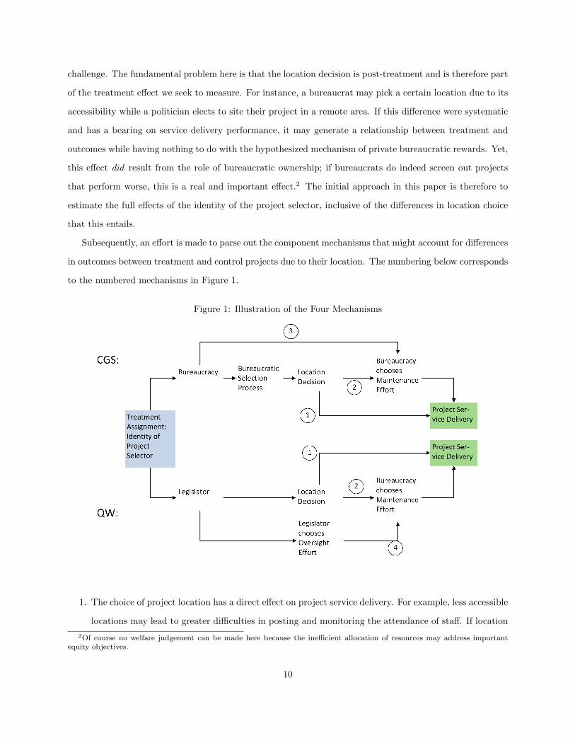
Subsequently, an effort is made to parse out the component mechanisms that might account for differences

in outcomes between treatment and control projects due to their location. The numbering below corresponds

to the numbered mechanisms in Figure 1.

Figure 1: Illustration of the Four Mechanisms

1. The choice of project location has a direct effect on project service delivery. For example, less accessible

locations may lead to greater difficulties in posting and monitoring the attendance of staff. If location

2Of course no welfare judgement can be made here because the inefficient allocation of resources may address importantequity objectives.

10

choice differed systematically across the CGS and QW this would produce a potential difference in ser-

vice delivery outcomes. One reason why choices might vary systematically is because bureaucrats have

private information about the costs and benefits of specific locations, and the process of bureaucratic

location selection ‘screens’ out the less promising projects in a way that legislator selection cannot.

2. Bureaucratic allocation of maintenance effort may respond to specific location choices, independent

of the identity of the project selector. For instance, where the legislator tends to locate projects in

opposition-dominated areas, the bureaucracy may have a political bias towards the incumbent that

leads them to reduce maintenance effort in those locations. This mechanism captures the ‘screening’

effect of bureaucratic decision-making, since bureaucratic contestation and consensus-building would

reduce the likelihood that such a project would receive funding. Note, however, that it is not the

identity of the project proposer, but simply the location of the project which is creating a difference

in service delivery outcomes here.

3. Bureaucratic allocation of maintenance effort may respond to the identity of the project selector,

independent of the location decision actually taken. This mechanism focuses on the reputational and

normative theories described above. Where bureaucrats participate in a project location decision, they

may subsequently exert more effort if they know that they will be able to claim greater credit and

personal rewards for the project than if the legislator had initiated the project. Alternatively, they

may simply develop a stronger normative attachment to a project in the process of selecting it and

this carries over to the maintenance stage.

4. In anticipation of the bureaucrat’s selection of lower effort for projects selected by the legislator, the

legislator chooses to exert higher effort to monitor the bureaucrat and raise the personal costs they

face in failing to maintain a project.

While the aggregate treatment effect incorporates all four mechanisms, it is helpful to try and disentangle

the mechanisms in order to identify which theory best accounts for the effects.

The first mechanism, based solely on systematically biased location choices which directly affect project

performance, reflects objective features of the location rather than decisions by the bureaucracy. For this

reason, it may be possible to control for key locational characteristics that might affect subsequent service

delivery performance. These covariates are included in follow-up models in order to parse out the differ-

ent mechanisms. In particular, altitude, terrain, infrastructure access, population size, population density,

distance to Local Government headquarters, distance to State capital, and the prior distribution of service

11

delivery facilities are used to capture features that would compromise service provision regardless of the

amount of effort that the bureaucracy invested in maintenance. To the extent that these variables are not

comprehensive, the resulting estimates will be biased and fail to partial out this mechanism.

The second mechanism primarily captures politicized allocation of maintenance effort by the bureaucracy.

If a legislator chooses to systematically locate projects in areas the bureaucracy has no interest in supporting,

maintenance effort will be low. A local measure of political affiliation would be needed to partial out this

mechanism. At present no such measures are available.

As a result, the residual effect having incorporated these two methodologies can be argued to reflect

the effect of the third and fourth mechanisms, namely the role of credit-claiming and normative attachment

to projects that induce bureaucrats to maintain projects they have selected themselves, and the role of

legislative oversight in holding bureaucrats accountable for effort in maintaining legislator-proposed projects.

Since these two effects are defined in opposition to each other it is not possible to separate them from each

other. However, the sign and magnitude of the residual effect should provide some indication of which of

the two mechanisms is dominant.

5.3 Strategic Interaction

A principal concern with the identification strategy above is that by simultaneously observing both the

treatment and control conditions operating at the same time on separate pots of funding, the experimental

ideal of observing a single pot of funding separately under treatment and control conditions is not replicated.

In particular, the very presence of both pots at the same time may alter the behaviour of the actors involved

because of strategic interaction with the choices of the other.

To give an example, the presence of both pots of funding may induce a degree of political competition

between bureaucratic and legislative initiators that would not be present if only one project were being

initiated. While this is certainly possible, this circumstance of dual selection is commonplace, and estimating

a treatment effect for circumstances where both bureaucrats and legislators are selecting projects does not

provide too much of a limitation.

A more serious challenge might be that location selection is not independent such that there is a violation

of the Stable Unit Treatment Value Assumption (SUTVA). If a bureaucratic selector identifies first a location

that the legislator would otherwise have chosen, the legislator may have to settle for a less appropriate

location which may have a lower intrinsic performance potential than the preferred site. This implies that

the potential outcomes for the QW project are affected by treatment in the form of the CGS project (and

12

vice versa). This possibility is a serious one that cannot be discounted. There are three potential mitigating

defences. First, while this may hapen for individual projects, it is not clear that there will be a systematic bias

in project selection. Indeed, sequencing is quite variable, with project selection an ongoing task overlapping

between the two schemes, and repeated over multiple years. Second, that the number of potential sites for

projects with equally high-performing potential is largely unconstrained given the substantial service delivery

gaps that exist in the country. Choosing an alternative site need not affect potential outcomes in this case.

Third, even if such displacement occurs, bureaucrats must still allocate maintenance resources between the

full portfolio of facilities, and if the effect operates through locational attributes we may be able to control

for such differences using locational data as described in the previous section.

5.4 Resource Allocation Between Areas

In precipitous circumstances, the two pots of funds would have been made available in each and every

Local Government for expenditure only within their boundaries. Then, the comparison is how the same

Local Government bureaucracy responded to the presence of two projects differing only (ideally) in project

selection. In practice, both pots may be diverted between Local Governments. On the one hand, CGS

projects are packaged by State Governments, who may reallocate resources between Local Governments. On

the other hand, QW projects are allocate by federal legislators whose constituencies encompass multiple Local

Governments. If different Local Governments always receive projects from different pots, the choice of where

to allocate maintenance resources is never made, and the effect we seek to estimate is spurious. In practice,

this concern is overcome by the fact that multiple projects are sited each year from each pot, such that

every Local Government (with just two exceptions, which are to be dropped) contains at least one project

from each pot. Thus, it is always possible to make a meaningful comparison where a real allocative choice

was faced by the local bureaucracy. Provided there are no spillovers or economies of scale between projects

from the same pot (and there is little reason to believe such spillovers would be pot-specific), an imbalance

in the number of projects from each project implemented in a particular Local Government introduces no

immediate source of bias under the matching specification where facilities within the same Local Government

are compared. Similarly, the use of fixed effects for Local Governments in some of the regression specifications

focuses attention on the within-Local Government variation between facilities, such that the allocation of

more projects from a particular pot to a particular Local Government need not introduce any source of bias.

13

6 Data and Measurement

To measure service delivery outcomes, I take advantage of a comprehensive survey (near-census) of health,

education and water supply facilities in Nigeria conducted between March 2011 and November 2012. This

dataset provides detailed information on the services provided by each facility and its operating conditions.

Interviews with the head of each facility and objective assessments by enumerators captured extensive and

detailed information about the nature and quality of services being delivered, although assessment was

restricted to a single unannounced visit.

Unfortunately, the dataset does not identify the funding source (which would enable identification of the

selector as a bureaucrat for the CGS and a legislator for the QW). However, information on the geographic

coordinates of each facility enables me to cross-reference the dataset with a separate survey that does capture

funding source. The two datasets are matched so that projects of the same type, with geographic coordinates

within 60m of each other, and with an altitude within 10m of each other, are assumed to be the same facility.

Information on key covariates is collected from GIS datasets, including altitude, distance measures, Nunn

and Puga’s (2011) measure of terrain ruggedness and population density from the Landscan dataset (Oak

Ridge National Laboratory 2011 ).

A large number of outcome variables are available and are listed in Table 1 below. These outcomes will be

used as alternative dependent variables, and due to the number of comparisons being made, the Bonferroni

adjustment will be made to the significance level to account for the possibility of chance significant results.

It should be noted that these output-based measures of service delivery are preferred over outcome-based

measures such as mortality rates or disease incidence in order to focus more closely on the role of government

in maintaining and operating the facility, and to avoid the complications introduced by differential local

health burdens or water stresses.3

For the water sector, the number of observations available is approximately 10,304. 75% of these are

under the treatment condition (CGS) and 25% are under the control condition (QW).

3The counterargument for using outcome-based measures is that personal rewards to bureaucrats and legislators may bebased on community outcomes rather than outputs, and that it is outcomes that therefore really motivate bureaucrats. Inpractice, the difficulties for communities in attributing responsibility for outcomes, and the relatively easy observability offacility outputs suggests that the latter may still carry considerable weight in this mechanism.

14

Table 1: Dependent Variable MeasuresHealth WaterNumber of days with no access to potable water last month? Reasonable Condition (new or

well maintained)? (dummy)Number of days without electricity in past month? Pay for water? (dummy)All weather road? (dummy) Lift mechanism automated (so-

lar, diesel, electric)? (dummy)Reasonable Health Facility Condition (new or not new but wellmaintained)? (dummy)

Missing fuel or electricity, condi-tional on being powered?

Wages have been paid in the last month? Multiple distribution points?(dummy)

Payment required for a routine visit ?Vaccine store present? (dummy)Access to improved sanitation/toilet (flush, VIP, pit latrine withslab)Staffing - three indicators (i) Number of nurses and higher,(ii) Number of medical staff down to junior chews,(iii) Total staff (including lab/records officersProvides child health services? (Dummy)Facility open 24/7? (dummy)Antenatal Care? (Dummy)Available anti-malarials, conditional on providing them as a policyThermometer available? (Dummy)Syringes available? (Dummy)Basic Emergency Obstetric Care? (Dummy)

7 Methodology

7.1 Regression Models

In applying the above identification strategy, the immediate comparison is between the average performance

of CGS and QW projects nationwide. Projects are therefore grouped by project type to enable comparison

of the dependent variable (construction of clinic, handpump borehole, solar-powered borehole etc.). This

facilitates a basic comparison of mean outcomes between the treated and control groups using a simple

regression. The only covariate included at this stage is the average evaluation score of the state government

in its project application to attempt to control for bureaucratic capability and its impact on the number of

projects implemented.

To isolate the three distinct mechanisms that could account for any effect, additional covariates are

then introduced.4 The covariates associated with pure location effects (mechanism (1)) are included. This

ensures comparison between projects that share similar locations in terms of their potential for service

4While many of these variables are ‘pre-treatment’ they introduce selection only through the location decision made by thebureaucrat/legislator which is post-treatment and so are not included in the earlier regression.

15

delivery performance.

The resulting estimate of the treatment effect on the treatment variable (CGS vs. QW projects) is

therefore expected to capture any residual difference arising from credit-claiming or normative attachment

to a bureaucrat-proposed project. As noted above, however, this estimate may be contaminated to an

unknown degree by unmeasurable variables, ad in particular the political allocation of resources between

locations by the bureaucracy which I am unable to control for.

The final regression equation is as follows. i is an observation in Local Government j. Y is any one of

the outcome measures, D is the treatment variable (CGS vs. QW project), X is the vector of covariates and

φ is the fixed effects for each Local Government. α is then the treatment effect for bureaucratic ownership.

Yij = β0 + αDij + βXij + γφj + εij (1)

For the full sample, power calculations suggest that relatively small deviations in the outcome indicators

should be detectable. Specifically, assuming a significance level of α = 0.05, a power of β = 0.8, and using

the true value for the proportion of treated units in the sample (0.75), Figure 2 illustrates how the minimum

detectable effect size, standardized into standard deviations of the outcome variable, varies for different

sample sizes. Encouragingly, for the case of the water sector, where 10,304 observations are available, this

suggests that an effect size of a 0.1 standard deviation change in the outcome indicators should be detectable.

7.2 Matching Estimates

The preceding discussion of identification challenges highlighted a number of concerns, but perhaps the most

central is the potential for strategic interaction and spillovers between projects. While it is unclear which

direction of bias may be introduced, the regression estimates are vulnerable to any such bias. Part of the bias

that reflects differences in geographic location may be netted out by controlling for key geographical variables.

However, the main reason that spillovers may arise is for local political reasons, and we are never likely to

have sufficient covariate information to control for this. Accordingly, I propose an alternative approach

which seeks to minimize the risk of spillovers by preventing such local comparisons. While still leveraging

on the comparison between the parallel pots of funding, the intention is to rely on the fact that while both

pots were implemented nationally, spillovers are, by definition, only significant for two locally proximate

projects. Therefore, a bureaucrat-selected project initiated in region A and a legislator-selected project

initiated in region B are unlikely to influence the potential outcomes of each other through any spillover.

16

Figure 2: Power Calculations

0 5000 10000 15000 20000

0.0

0.1

0.2

0.3

0.4

0.5

Sample size

Sta

ndar

dize

d M

inim

um D

etec

tabl

e E

ffect

Siz

e

The comparison between these two projects is therefore potentially more reliable than a local comparison.

Of course, the reason that local comparisons are typically preferred is because other background conditions

are more likely to be held constant across projects. This approach therefore places a particularly strong

burden on controlling for a wide range of relevant background covariates.

To implement this proposal, matching is the most appropriate design. This allows us to pair particular

projects for comparison, using a large number of covariates to achieve close matches. However, the primary

matching criteria is that projects must be at least a fixed geographic distance form each other, say 100km,

such that there is no potential for logistical or political spillovers. Matching is to be conducted using a

variety of algorithms to achieve optimal balance across the treatment and control groups. In the water

sector, since there are three CGS projects for every QW project, multiple matches are permitted. The

post-matching regressions then facilitate estimation of treatment effects. This strategy also places greater

reliance on the comparability of projects across Local Government contexts, since we are explicitly comparing

a project under bureaucratic ownership in the domain of one Local Government with a project under political

ownership in the domain of another Local Government. Since these Local Governments may vary in their

underlying capacity for service delivery, achieving balance on this characteristic across the dataset relies on

17

having a balanced distribution of projects between Local Governments. As noted earlier, there are reasons

to think this may be largely the case, and that measured covariates (for example, average project evaluation

score) can be used to control for any residual imbalance.

This matching approach - if adequate balance can be achieved on other characteristics - may go a

significant way to addressing the concern of local spillovers by ruling out potentially spurious relationships

generated by local spillovers between projects. However, the approach is by no means foolproof - if there is a

systematic pattern across Local Governments in the way that spillovers operate then this will be reflected in

the treatment estimates. If, for example, politicians implicitly get ‘first-call’ on project sites, then they may

be able to select their preferred sites at the expense of bureaucrats. If these differences in turn affect service

delivery they will bias the treatment effect even when we compare projects in different regions. While there is

no specific evidence of any such directional bias, the possibility is a persistent challenge to the identification

strategy outlined above.

References

Barro, R J. 1973. “The Control of Politicians: An Economic Model.” Public Choice 14:19–42.

Booth, David. 2003. “Introduction and Overview.” Development Policy Review 21(2):131–159.

URL: http://doi.wiley.com/10.1111/1467-7679.00203

Boughton, James M. and A. Mourmouras. 2002. “Is Policy Ownership an Operational Concept?”.

Carpenter, Daniel P. 2010. Reputation and Power. Princeton University Press.

Federal Government of Nigeria. 2006. Core Welfare Indicators Questionnaire. Technical report.

Federal Government of Nigeria. 2010a. MDG Report 2010. Technical report.

Federal Government of Nigeria. 2010b. “Partnering to achieve the MDGs: The Story of Nigeria’s Conditional

Grants Scheme.”.

Haggard, Stephen and Robert R. Kaufman. 1992. The Politics of Economic Adjustment: International

Constraints, Distributive Conflict and the State. Princeton University Press.

Heider, F. 1958. The Psychology of Interpersonal Relations. New York: Wiley.

Kaufman, Herbert. 1960. The Forest Ranger: A Study in Administrative Behaviour. Routledge.

18

Keefer, P. and R. Vlaicu. 2007. “Democracy, Credibility, and Clientelism.” Journal of Law, Economics, and

Organization 24(2):371–406.

URL: http://jleo.oxfordjournals.org/cgi/doi/10.1093/jleo/ewm054

Killick, Tony, Ramani Gunatilaka and Ana Marr. 1998. Aid and the Political Economy of Policy Change.

Lemarchand, Rene. 2012. “Political Clientelism and Ethnicity in Tropical Africa :* Competing Solidarities

in Nation-Building.” American 66(1):68–90.

Nunn, Nathan and D Puga. 2012. “Ruggedness: The Blessing of Bad Geography in Africa.” Review of

Economics and Statistics 94(1):20–36.

Oak Ridge National Laboratory. 2011. “LandScan Global Population Database.”.

URL: http://www.ornl.gov/sci/landscan/

OECD. 2008. “Paris Declaration on Aid Effectiveness.” pp. 29–41.

of Nigeria, Federal Government. 2011. Survey of Civil Servants: Voices from the Service. Technical report.

Stiglitz, Joseph E. 2002. “Participation and Development: Perspectives from the Comprehensive Develop-

ment Paradigm.” Review of Development Economics 6(2):163–182.

URL: http://doi.wiley.com/10.1111/1467-9361.00148

Wantchekon, Leonard. 2012. “Clientelism and Voting Behavior : Evidence from a Field Experiment in

Benin.” World Politics 55(3):399–422.

19