Embed Size (px)
Citation preview

Does Corporate Governance Induce Earnings Management?
Evidence from Bonus Depreciation and the Fiscal Cliff∗
Eric Ohrn†
Grinnell College
December 2014
Abstract
Corporate governance mechanisms can improve managerial performance, but may encourage
managers to focus on current financial statement earnings at the expense of long-run profits.
This unintended effect is revealed by reactions to “bonus depreciation,” a U.S. tax policy that
reduces tax expense without improving reported earnings. During 2000–2010, investment by
better-governed firms responded less to bonus depreciation than did firms with less effective
governance. Similarly, share prices of poorly governed firms reacted most strongly to the surprise
2013 extension of bonus depreciation. Taken together, these results suggests that high-powered
managerial incentives encourage earnings management behavior.
Keywords : Corporate governance, earnings management, bonus depreciation
JEL Codes: H25, G31, G30
∗I thank my dissertation committee James Hines, Christopher House, Joel Slemrod, and Justin Wolfers; as well
as Jesse Edgerton, Max Farrell, John Friedman, Michael Gideon, Jason Hall, Kevin Hassett, Pawel Krolikowski, Tom
Neubig, Amiyatosh Purnanandam, Nathan Seegert, and Bryan Stuart; for very useful feedback. I am also grateful to
seminar participants at the University of Michigan for helpful suggestions. All errors are my own.†[email protected]
1
1 Introduction
Economists have long understood that the actions of publicly traded corporations are greatly in-
fluenced by a separation of firm ownership and control. Shareholders, the owners of the firm, hire
professional managers to control firm operations and make decisions on their behalf. This sep-
aration can give rise to a principal–agent problem if the objectives of the professional managers
differ from those of the shareholders. These problems can be difficult to solve because shareholders
cannot perfectly observe and evaluate the managers’ decisions.
However, firm ownership can look towards corporate governance mechanisms, such as threat
of takeover, discretionary payments, or equity packages, to align the objectives of the managers
with their own. While strong corporate governance has the ability to align objectives and move
the firm towards actions that are optimal for the shareholders, it may also generate an unintended
and counterproductive side effect; strong corporate governance places pressure on managers to
signal their value to shareholders by manipulating performance metrics that are easily observable
to shareholders.
Evidence indicates that in the corporate context there is a single most salient performance
metric: “accounting earnings” or the bottom line number on a firm’s income statement.1 Because
investors fixate on accounting earnings, managers facing strong corporate governance pressure are
incentivized to manipulate accounting earnings possibly at the cost of long-term real economic
benefits to the firm, a behavior known as “earnings management.”2
The canonical example of earnings management behavior is the delay or cancellation of positive
net present value investments because the project may adversely affect accounting earnings. In
addition to investment, earnings management may distort firm financing and payout decisions,
thereby depressing firm values and significantly impacting welfare for the economy as a whole.3
Thus, while strong corporate governance may move the firm towards optimal behavior, it does so
at the cost of increasing earnings management.
Despite the strong intuition, theoretical underpinnings, and anecdotal evidence that corporate
governance induces earnings management, empirical analyses have not been able to confirm the
hypothesis for two reasons. First, identifying instances in which managers choose to increase current
accounting earnings by altering firm behavior is difficult. Second, levels of corporate governance
and earnings management behavior are potentially simultaneously determined.
I rely on a corporate tax policy, “bonus depreciation,” to address these issues and formally
1Publicly traded firms in the United States are required to prepare income statements under Generally AcceptedAccounting Principles (GAAP). Audited income statements appear on firms’ annual 10K financial reports.
2The accounting literature distinguishes two types of earnings management. Managers that manipulate discre-tionary information on financial statements, such as loan loss provisions, engage in “accruals management.” Managersthat alter firm behaviors to manipulate financial reporting engage in “real earnings management.” In this research,I focus on the relationship between corporate governance and real earnings management.
3Stein (1989) shows that earnings management behavior can exist even in the context of efficient capital markets.
2
test whether corporate governance induces earnings management behavior. Bonus depreciation is
a largely counter-cyclical corporate tax incentive that has been the primary investment stimulus
tool in use in the US over the last decade. Bonus depreciation decreases the net present value cost
of investment projects by accelerating the deduction for the costs of newly installed capital from
taxable income.
While bonus depreciation effectively increases the economic value of investment projects, it
leaves the accounting earnings associated with any potential project unchanged. Under Generally
Accepted Accounting Principles (GAAP), the cost of new investments appears on the earnings
statement only as the new capital investment is used up or economically depreciates over the life
of the investment. Because the rate at which new capital economically depreciates is unaffected by
tax depreciation rules, bonus depreciation does not affect the cost of investment on the earnings
statement and therefore leaves accounting earnings unchanged.4 This accounting treatment of
bonus depreciation provides exogenous variation that can be used to identify earnings management
behavior and test the governance hypothesis.
If managers seek to maximize only accounting earnings, then bonus depreciation has no effect
on their objective function and does not alter their behavior. Alternatively, for managers that
seek to maximize the economic value of the firm, bonus depreciation provides strong incentives
for increased investment. The absence of response (or under-response)to the policy is evidence of
earnings management. If the investment behavior of strongly governed firms is less responsive to
bonus depreciation, then it can be interpreted as evidence that earnings management is a side effect
of corporate governance practices. This research design avoids the simultaneity complications under
the plausible assumption that corporate governance decisions are not made based on investment
response to the tax policy.
Exploring heterogeneity of response among firms with varying levels of governance is exciting
not only in that it may confirm earnings management as an unintended consequence of strong
corporate governance but also from a tax policy perspective. Use of bonus depreciation and the
design of the policy itself may have to be reconsidered in light of heterogeneous response especially
considering the staggering magnitude of the policy: estimates suggest that in 2011 alone bonus
depreciation stimulated approximately $50 billion in new investment.
2 Related Literature
2.1 Corporate Governance
Since the 1970’s, an active literature has developed that addresses the role of corporate governance
in solving principal–agent problems of the firm. The first papers in the literature detailed how
4The discrepancy between the timing of expenses for tax and financial reporting purposes is recorded as the“temporary book-tax difference” on financial statements.
3

the separation of ownership and control within the firm affects firm behavior. Jensen and Meck-
ling (1976) examined the impact of the agency problem on the method of finance. Grossman and
Hart (1980) described its effects on takeover bids. Easterbrook (1984) formalized how dividend
policy was altered in an agency setting. Later research examined possible solutions to these agency
problems. Jensen (1986) suggested that the use of debt financing may discipline suboptimal in-
vestment behavior arising from abuse of free cash flows by self-interested managers. Shleifer and
Vishny (1986) argued that large minority shareholder can overcome freeriding problems in effective
monitoring of management and thereby mitigate agency problems. Jensen and Murphy (1990)
empirically explored pay-for-performance incentives and their ability to align the incentives of top
executives with those of the owners. The general conclusions of these studies were that agency
costs were high and various governance mechanisms such as debt financing, strong monitoring, and
incentive pay can and should be increased.
More recent empirical evidence has reinforced these conclusions. Bertrand and Mullainathan
(2003) used exogenous decreases in corporate takeover probability to show that when managers are
less subject to the threat of takeover, they prefer to “live the quiet life” and decrease effort-intensive
investment behavior. Gompers, Ishii and Metrick (2003) combined 24 governance provisions into an
index that proxies for the strength of shareholder rights and found that equity returns for firms in
the top decile of the index are larger than for firms in the bottom decile, suggesting that, over time,
firms with better corporate governance perform better. Bebchuk, Cohen and Ferrell (2009) reduced
the Gompers et al. (2003) index to the six provisions that truly matter from a legal perspective
and found that Tobin’s Q, a measure of firm performance, monotonically decreases when managers
are subject to less strict shareholder governance. 5
While the majority of empirical results have highlighted the benefits of stronger governance,
Jensen (2004) suggested that equity incentives may lead to unintended, counterproductive conse-
quences. Jensen (2004) considered the effect of high managerial equity incentives when analysts
project high earnings and stock prices are overvalued. Overvaluation places pressure on managers
to increase accounting earnings often at the cost of real economic value. Jensen pointed out that the
pressure to engage in earnings management behaviors to artificially inflate earnings to hit targets
increases as management owns a larger portion of outstanding equity.
2.2 Earnings Management
Healy and Wahlen (1999) defined earnings management as “when managers use judgment in finan-
cial reporting to alter financial reports to either mislead stakeholders about the underlying eco-
nomics performance of the company, or to influence contractual outcomes that depend on reported
numbers.” In their review they conclude that empirical evidence is consistent with firms altering
5I will make use of both the Gompers et al. (2003) “G Index” and the Bebchuk et al. (2009) “Entrenchment Index”in the empirical analysis presented in Section 6 and Section 7.
4
financial statements via discretionary accountings of loan loss provisions and abnormal accruals
prior to public securities offerings, to avoid violating contracts and increase corporate managers’
compensation and job security (For an additional review of the earnings management literature,
see Dechow and Skinner (2000)). In short, managers alter earnings by the use of discretionary
accounting exactly when earnings mean the most to the firm.
While discretionary accounting may mislead investors, a more concerning type of earnings
management is detailed in survey evidence by Graham, Harvey and Rajgopal (2005). The authors
survey more than 400 corporate financial executives on the relationship between equity perfor-
mance and real business decisions. The responses show that the majority of financial managers
believe the key metric in evaluating firms’ performance is earnings (especially earnings per share),
not cash flows. Additionally, they find the majority of respondents would not initiate a positive
net present value project if it meant falling short of the current quarters’ earnings projection and
would give up economic value in exchange for smooth earnings performance. The respondents
described a general trade-off between the need to “deliver earnings” and the making of long-run
value-maximizing decisions. This survey evidence suggests not only that managers might use dis-
cretionary accounting practices to mislead shareholders, but also that they are pressured to distort
real firm behaviors in order to manipulate short term accounting earnings. If the need to deliver
accounting earnings affects real business decisions, then earnings management behaviors may have
significant consequences for the long-run firm values and by extension for the economy as a whole.
Empirical evidence from the stock market supports the beliefs and actions of the corporate
managers included in the survey. Sloan (1996) investigated the relationship between stock prices
and movement in different financial indicators. He found that stock prices move in patterns that
suggest that investors “fixate” on accounting earnings; stock prices do not reflect information con-
tained in accruals or cash flows that impact only future earnings. Given this fixation on accounting
earnings relative to other measures of future profitability, it is not surprising that corporate man-
agers manipulate earnings via changes in discretionary accruals and long-run profit-maximizing
behavior.
Erickson, Hanlon and Maydew (2004) provided an example of firms sacrificing real economic
value to increase accounting earnings. They examined a sample of 27 firms that paid a total of $320
million dollars of real cash taxes on earnings that were later alleged to be fraudulent. Shackleford,
Slemrod and Sallee (2011) noted several other empirical explorations of real earnings management
behavior and have taken the first steps towards modeling a firm that alters real economic activity
to maximize a function of accounting earnings.
2.3 Governance and Earnings Management
Stein (1989) suggested that earnings management can exist in an efficient capital market and may
be a function of governance. Stein suggests that short-run earnings manipulation at the cost of
5

long-run real economic benefits can be viewed as the Nash Equilibrium outcome of a game between
managers and the stock market. To induce the market to predict higher future earnings, managers
engage in costly behaviors to improve short-term accounting earnings. In equilibrium, the mar-
ket is not fooled by the enhanced short-run earnings, but the behavior persists because deviating
from the equilibrium is strictly dominated from the perspective of the manager. Furthermore, the
weight the manager places on short-term accounting earnings increases in the threat of takeover
and the proportion of managerial compensation that is derived from equity incentives: two gover-
nance mechanisms. Crucially, as corporate governance measures are increased, the incentives for
unintended counter-productive earnings management behavior are stronger.
A limited empirical literature has tested theories related to the Stein (1989) hypothesis that
corporate governance increases focus on short-run accounting earnings. Meulbroek, Mitchell, Mul-
herin, Netter and Poulsen (1990) tested this hypothesis by examining research and development
activity, a behavior which reduces short-term earnings but may lead to increased future profits.
They found that anti-takeover measures reduce R & D spending, an empirical result that contradicts
Stein’s model but may be driven by the “quiet life” theory of governance addressed in Bertrand
and Mullainathan (2003). More recent evidence also contradicts Stein’s hypothesis. Klein (2002)
found that when audit committees or boards are independent of executive management, abnormal
accruals are smaller. Xie, Davidson III and DaDalt (2003) and Zhao and Chen (2008) find that
audit committee expertise in accounting, the frequency at which the board and audit committees
meet, and staggered boards, another takeover defense, all decrease use of discretionary accruals.
2.4 Investment and Taxation
To test for earnings management behavior, I will rely on the theoretical and empirical tools devel-
oped to explore the impact of tax policy on investment behavior. Summers (1981), Poterba and
Summers (1985), and Desai and Goolsbee (2004) built on the seminal Hall and Jorgenson (1967)
paper and estimate models which measure investment as a function of marginal Q and a term that
combines corporate income taxation, investment tax credits, the rate of tax depreciation, interest
rates, and real rates of economic depreciation into a single “user cost of capital” measure. I utilize
a modified user cost model to test the relationship between corporate governance and earnings
management behavior.
2.5 Accelerated and Bonus Depreciation
When a firm invests in new capital, it can deduct the purchase price of the investment from its
taxable income, thereby reducing its tax bill. In most cases, the firm cannot deduct the entire
amount immediately. Under US law, the schedule of depreciation deductions is specified by the
Modified Accelerated Cost Recovery System (MACRS). For each type of property, MACRS spec-
6
ifies a recovery period and a depreciation method that specifies how quickly and over what time
frame the purchase price is to be deducted. When the rate of depreciation for tax purposes is
faster than the true rate of economic depreciation on capital investments, depreciation is said to be
“accelerated.”6 Accelerated depreciation decreases the user cost of capital and effectively creates a
tax subsidy on new equipment purchases.7 While the US Government has used accelerated depreci-
ation to encourage investment for more than 50 years, it has only recently employed the policy in a
counter-cyclical manner (Gravelle (2013)).8 “Bonus depreciation,” the counter-cyclical manifesta-
tion of accelerated depreciation, is unique in its magnitude and its temporary nature. Under bonus
depreciation, businesses can write off a specified percentage of new purchases immediately, thereby
further accelerating depreciation and increasing the investment tax subsidy. Bonus depreciation
was used to combat both the 2001 and the 2008 recessions and has been the primary tool used
to stimulate business investment during the last decade. The White House estimates that bonus
depreciation saved businesses approximately 55 billion present value dollars in corporate income
taxes in each of the years 2010 and 2011.9
Much evidence suggests that business investment does respond to bonus depreciation, although
as noted by House and Shapiro (2008), investment elasticity estimates are surprisingly small, given
the temporary nature of the policy. The authors note that with price elasticity of supply and
adjustment costs equal to zero, the elasticity of investment with respect to the changes in investment
cost via temporary bonus depreciation should be infinite. Finding limited investment and supply
price response, House and Shapiro conclude that convex adjustment costs within the firm must
mute the investment response.
The notion that bonus depreciation can identify earnings management behavior and can be used
to test for the relationship between corporate governance and earnings management began with
Neubig (2006), which suggested an alternative explanation for the tempered investment response to
the policy. Neubig pointed out that, due to GAAP, bonus depreciation does not affect accounting
earnings. If firms, as the earnings literature suggests, seek to maximize accounting earnings as
opposed to net present value of cash flows (real economic value), their investment behavior will
be unresponsive to bonus depreciation. Therefore, unresponsiveness in the face of the policy is
evidence of earnings management behavior; firms focusing on accounting earnings do not increase
investment despite a substantial subsidy.
6The “true” rate of economic depreciation is how quickly the new capital actually deteriorates or is “used up.”7In order for bonus depreciation to decrease NPV costs of investment, the firm must have positive taxable income.
Heterogeneous response by firms with different tax statuses is examined in Appendix J. Results continue to exhibitstrong heterogeneous investment response across governance levels.
8In 1954, depreciation rules were liberalized explicitly“to maintain the present high level of investment in plant andequipment” (Senate Finance Committee, quoted in Brazell, Dworin and Walsh (1989)). Legislation has changed thedepreciation rules several times since then, but the intention to encourage investment through accelerated depreciationhas persisted.
9In 2010, businesses could immediately deduct 50% of the cost of new investments; in 2011, 100%. When allequipment is immediately fully deductible, it is known as “expensing.”
7
Edgerton (2012) formalized Neubig’s intuitive and elegant explanation for the relatively small
elasticity and constructed a model of a firm that focuses attention on both true economic value
and accounting earnings. By observing investment responses to different types of investment tax
incentives that both do and do not affect accounting earnings, Edgerton estimateed that the average
firm focuses 45% of their attention on accounting earnings and 55% of their attention on cash flows
when making investment decisions.10
3 Modeling Governance and Investment Response to Bonus
Depreciation
In this section, I build governance into the formal model of investment behavior presented in
Edgerton (2012), in which managers make investment decisions to maximize a weighted sum of
cash flows and accounting earnings. The key innovation of the model is that the weight placed on
accounting earnings is a function of the strength of governance faced by management. The formal
model generates a linear estimating equation that embodies the intuitive prediction that managers
under strong corporate governance face high pressure to maximize accounting earnings and are
therefore less responsive to bonus depreciation.
3.1 Model Preliminaries
Firms maximize a weighted average of their current and future present value net-of-tax cash flows
(CFt) and their accounting earnings (AEt). Investment is financed using retained earnings.11 The
definition of cash flows is
CFt = (1− τ)[F (Kt)− pψ(It,Kt)] + τδTKTt − pIt,
where τ is the corporate tax rate and p is the unit price of capital. F (·) is the net operating income
function and is a function of Kt, the firm’s capital stock. ψ(·) is the adjustment cost of investment,
which is a function of It, investment, and capital stock. The firm’s capital stock evolves according
to the law of motion,
K̇t = It − δKt (1)
10Also see Edgerton (2012) for a comprehensive explanation and examples of how and why bonus depreciationeffectively decreases net present value but leaves the accounting earnings associated with any given investmentproject unchanged.
11The model can be extended to include debt finance with relative ease. Investment policy is identical when thefirm invests with retained earnings or a combination of retained earnings and debt.
8
where δ is the real depreciation rate of the capital stock.12 The cost of new investment, It, is
pIt.13,14
In addition to investment tax credits, the depreciation deductions permitted for tax purposes
enter into the cash flow definition and may encourage investment behavior. These deductions are
a function of the stock of the firm’s past capital expenditures that have not been depreciated for
tax purposes, KTt , and the statutory tax rate of depreciation, δT . I will refer to KT
t as the “tax
capital” of the firm. Tax capital evolves according to the law of motion,
K̇Tt = pIt − δTKT
t . (2)
The tax savings afforded by these deductions appears in the cash flows equation as τδTKTt . The
policy parameter δT determines the extent to which depreciation is accelerated for tax purposes
and embodies the bonus depreciation policy.15
The firm’s accounting earnings are defined as
AEt = (1− τ)[F (Kt)− pψ(It,Kt)− δBKBt ].
Revenues F (Kt) and adjustment costs pψ(It,Kt) enter into both after-tax cash flows and account-
ing earnings identically. However, the cost of investment, pIt, and cash tax savings, τδTKTt , do
not appear in the accounting earnings equation at all. Instead, there appears a book measure of
12This law of motion formulation assumes geometric capital stock depreciation. In reality, capital stock maydepreciate at non-geometric patterns. This assumption is made for mathematic simplicity and does substantivelyinfluence the predictions of the model.
13If investment tax credits were offered, the investment would generate investment tax credits of pItITC. Thesecredits would enter into accounting earnings identically and, therefore, investment response to ITCs will not be afunction of α.
14The model abstracts from investment tax credits (ITCs) because they are not available to businesses duringthe estimation period. However, ITCs can be easily incorporated into the model. ITCs affect both cash flows andaccounting earnings identically and therefore investment response to investment tax credits does not depend on αor determinants of α. This observation provides another test that the observed empirical findings are generated bythe accounting treatment of bonus depreciation and is evidence of earnings management behavior. If investmentresponse to ITCs is not heterogeneous across governance levels then evidence of the corporate governance–earningsmanagement is reinforced.
Unfortunately, ITCs were last used in 1985 and corporate governance data is not available prior to 1991, so testsof this secondary hypothesis are challenging. However, in Appendix L, I use 1991 governance data in an attemptto measure the degree of heterogeneous investment response to both ITCs and depreciation tax allowances in yearssurrounding the ITC repeal. The analysis finds no heterogeneity of response across governance levels to the ITCrepeal. The absence of heterogeneity could be the result of either changes in within-firm governance between years1985 and 1991 or support of the ITC hypothesis. The analysis presented in Appendix L also finds no differences ininvestment response to changes in tax depreciation allowances. Again, this could be due to the poor measurement ofmid 1980s governance using 1991 data. Alternatively, this result could be due to the fact that changes in depreciationwere not nearly as salient as changes in bonus depreciation and were not the preeminent investment tax stimulusused during the 1980s, which were investment tax credits.
15This parameter is also assumed to be constant, and thus tax depreciation allowances are assumed to decline at ageometric rate. In reality, this is not the case. However, this abstraction does not substantively alter the predictionsof the theory.
9
depreciation deductions, δBKBt , and their associated tax savings, τδBKB
t . The cost of new invest-
ment only depresses accounting earnings as the capital depreciates for book purposes. Book capital
evolves according to its own law of motion,
K̇Bt = pIt − δBKB
t . (3)
Thus, bonus depreciation, which increases δT and decreases the cash flow cost of investment, does
not alter accounting earnings.
I assume the firm places a weight α on book earnings (AE) and a weight (1 − α) on after-tax
cash flows (CF) when choosing its investment. The firms solves
maxIt
∫ ∞0
e−rt[αAEt + (1− α)CFt]
subject to constraints (1), (2), (3), and (4).16
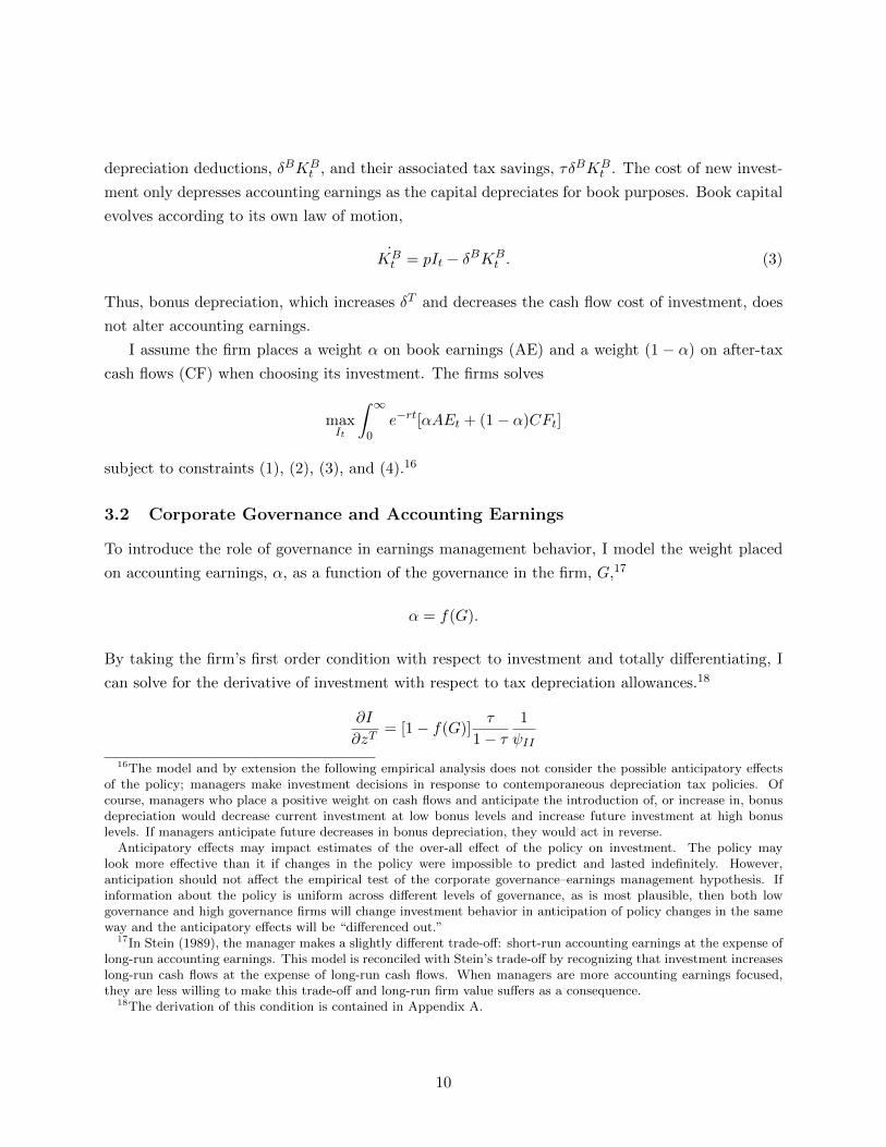
3.2 Corporate Governance and Accounting Earnings
To introduce the role of governance in earnings management behavior, I model the weight placed
on accounting earnings, α, as a function of the governance in the firm, G,17
α = f(G).
By taking the firm’s first order condition with respect to investment and totally differentiating, I
can solve for the derivative of investment with respect to tax depreciation allowances.18
∂I
∂zT= [1− f(G)]
τ
1− τ1
ψII
16The model and by extension the following empirical analysis does not consider the possible anticipatory effectsof the policy; managers make investment decisions in response to contemporaneous depreciation tax policies. Ofcourse, managers who place a positive weight on cash flows and anticipate the introduction of, or increase in, bonusdepreciation would decrease current investment at low bonus levels and increase future investment at high bonuslevels. If managers anticipate future decreases in bonus depreciation, they would act in reverse.
Anticipatory effects may impact estimates of the over-all effect of the policy on investment. The policy maylook more effective than it if changes in the policy were impossible to predict and lasted indefinitely. However,anticipation should not affect the empirical test of the corporate governance–earnings management hypothesis. Ifinformation about the policy is uniform across different levels of governance, as is most plausible, then both lowgovernance and high governance firms will change investment behavior in anticipation of policy changes in the sameway and the anticipatory effects will be “differenced out.”
17In Stein (1989), the manager makes a slightly different trade-off: short-run accounting earnings at the expense oflong-run accounting earnings. This model is reconciled with Stein’s trade-off by recognizing that investment increaseslong-run cash flows at the expense of long-run cash flows. When managers are more accounting earnings focused,they are less willing to make this trade-off and long-run firm value suffers as a consequence.
18The derivation of this condition is contained in Appendix A.
10

where zT , a transformation of δT , is the present value of future depreciation allowances for tax
purposes.19 When bonus depreciation is introduced or increased and tax depreciation allowances
are accelerated, zT increases. ψII is the second derivative of the adjustment cost function with
respect to investment. The investment response to the bonus depreciation decreases as more weight
is placed on accounting earnings. If f(G) is an increasing function of G, then investment response
to bonus depreciation decreases as the firm is more heavily governed.
3.3 Estimation
I approximate f(·) as a linear function,
α = γGG, (4)
where γG defines how governance affects the accounting focus parameter α. Under the assumption
of quadratic adjustment costs,20 the investment ratio may be expressed as a linear function,
I0K0
= a+ c
λ0p0− 1
1− τ+ c
τzT
1− τ− cγGGτz
T
1− τ+ c
(1− τzB)γGG
1− τ,
which can be estimated using ordinary least squares regression of the form
IitKi,t−1
= β0 + β1τzTit
1− τt+ β2
Git1− τt
+ β3Gitτz
Tit
1− τt+ β4
λitpit
1− τt+ εit.
During the sample period that I examine, the corporate income tax rate τ does not change. Under
these conditions, I can drop the corporate tax rates from the estimating equation and estimate
IitKi,t−1
= β0 + β1zTjt+β2Git + β3Gitz
Tjt + β4
λitpit
+ εit. (5)
The regression equation contains a tax term that describes the impact of the bonus depreciation
zT , a governance term, G, and their interaction as well as marginal Q (λit/pit). In order to account
for firm-level unobserved determinants of investment behavior and the endogenity of tax policy, I
add firm and year fixed effects to the regression.
Estimates from this linear regression can be used to test the corporate governance–earnings
management hypothesis. From (5), γG defines the relationship between governance and accounting
19See Appendix A for more details.20The canonical quadratic adjustment equation employed by Desai and Goolsbee (2004) and others is
ψ(It,Kt) =1
2c
[ItKt
− a
]2Kt,
where c is an adjustment cost parameter.
11
earnings focus. This parameter of interest can be constructed by taking a ratio of coefficients from
the regression, γG = −β3/β1. In intuitive terms, β1 is the response by firms with a “zero” level of
governance. β3 is the amount that the β1 coefficient changes when an additional unit of governance
is added. It follows that γG is the fraction that the investment response decreases when governance
increases by one unit relative to the response of the “zero” governance firms.
If γG is estimated to be positive, investment response to bonus depreciation is decreasing in
the corporate governance measure, and empirical evidence indicates that the weight placed on
accounting earnings is larger at higher levels of corporate governance. This result would strongly
support the hypothesis that corporate governance induces earnings management behavior consistent
with the evidence presented in Section 2.21
3.4 Endogenous α
One simple and plausible extension of the model would allow α to be a function of depreciation tax
benefits in addition to governance. The logic behind this assumption is that managers, knowing
that accounting earnings do not reflect the tax benefits of accelerated depreciation, may shift their
focus towards cash flows when bonus depreciation is enacted or increased to better take advantage
of the policy. With this extension, investment response to depreciation tax incentives would be
positive, but would decrease more slowly in the level of governance. Thus, if α is a function of
depreciation tax allowances, then the estimated γG from equation (5) would underestimate the
impact of governance on the accounting earnings weight α.
4 Data Construction and Descriptive Statistics
In order to examine the investment response to bonus depreciation across firms with different
levels of corporate governance, I collect data from the RiskMetrics Governance Legacy Database,
from the Standard and Poor’s Execucomp database, from Internal Revenue Service documentation,
from Bureau of Economic Analysis Capital Flows tables, and from Standard and Poor’s Compustat
CRSP combined database. The remainder of this section outlines the construction, measurement,
and descriptive statistics of key variables.
4.1 Governance Index
Following Gompers et al. (2003), I construct a firm level measure of governance based on the 24
governance provisions contained in the RiskMetrics Governance Legacy Database. The majority of
21The investment equation implies that changes in marginal Q (λ/p) should have the same impact on the investmentratio as the Z Tax Term. Unfortunately, because proxies for marginal Q are often mismeasured, this result is typicallynot present in Q-theory empirical studies. See Cummins, Hassett and Hubbard (1994) and Cummins, Hassett andOliner (2006) for potential solutions to the mismeasurement problem.
12
provisions recorded by Riskmetrics protect the manager from disciplinary actions on the part of the
shareholders or protect the firm from takeovers. Gompers et al. (2003) construct a “G Index” in a
simple, straightforward manner: for every firm, a point is added for every provision that restricts
shareholder rights. I transform the “G Index” in an effort to make its interpretation more intuitive.
To construct the “Governance” variable that I will use in the empirical analysis, I subtract “G
Index” for each firm and year from the maximum “G Index” observed in the data.
The transformed “Governance” variable has the advantage over the “G Index” that it is in-
creasing in proportion to the level of governance placed on the manager by the shareholders of the
firm. A one point increase in the Governance variable means that the firm has one fewer provision
in place to protect managers from shareholder discipline. For further ease of interpretation, I scale
Governance by its standard deviation over the sample period, so that a one point increase in the
standardized variable corresponds to a one standard deviation increase in governance relative to
the average level of governance observed in the data.2223
Bebchuk et al. (2009) constructed an “Entrenchment Index” from 6 of the original 24 provisions
that they found most important from a legal and operational standpoint.24 I transform and scale
their index in the same manner as the “G Index” to create “Entrenchment.” I use this measure as a
robustness check in Appendix D and in the fiscal cliff analysis because data necessary to construct
the Governance variable are unavailable.
Figure 1 presents a histogram of the Governance variable overlaid with a normal distribution.
The governance variable is normally distributed with a median value of 9 and standard deviation
of 2.557. Figure 2 compares Governance and Entrenchment across firms. The figure confirms that
firms with high Governance measures, on average, have high Entrenchment measures of corporate
governance.
4.2 Managerial Equity Percentage, “Shares”
The third measure of governance that I consider is the percentage of total shares held by the firm’s
highest-paid executive, which I label “Shares.” I use this measure for two reasons. First, it is used in
other papers, making my results comparable to an earlier literature. Second, results from Jensen and
Murphy (1990) suggest that fractional ownership is a close proxy for pay–performance sensitivity
for CEOs with non-negligible stockholdings. I follow Chetty and Saez (2005) in constructing this
22The G Index is available only for years 2000, 2002, 2004, and 2006. The Governance variable for years 2001, 2003,and 2005 is imputed as the value of the G Index for the previous year. The Governance variable for years 2007–2010is constructed from the 2006 G Index. Appendix E presents several robustness checks to confirm that this simpleimputation does not strongly influence empirical results. As Gompers et al. (2003) noted, there is little within-firmchange in the index over time, so it is unsurprising that these checks do not strongly influence results.
23Data on corporate governance provisions has been collected by RiskMetrics for years 2007 to 2011. However,these data do not contain the full swath of provisions examined in Gompers et al. (2003) and thus the exact G Indexcannot be constructed for these years.
24The Entrenchment Index focuses on 6 provisions: (1) Staggered Board, (2) supermajority to approve mergers,(3) limited ability to amend charter, (4) limited ability to amend bylaws, (5) poison pill, and (6) golden parachute.
13

Figure 1: Governance
(a) Distribution
05
1015
Per
cent
0 5 10 15 20Governance
(b) Governance and Entrenchment
02
46
Ent
renc
hmen
t
0 5 10 15 20Governance
Notes: Figure 1(A) presents a histogram of the Governance variable overlaid with a normal distribution. Panel(B) presents the linear fit relationship between the Government and Entrenchment variables as well as a binnedscatter plot of their relationship. The Governance variable is split into 17 equal-sized bins. For each bin, the averageEntrenchment is plotted. The linear fit is predicted over unbinned data.
measure using the following method: (1) for each firm, the top executives are ordered by total
compensation, then (2) the shares owned by highest-paid executive are divided by the total shares
of the firm to find the percentage of the firm held by the top executive.25 Shares owned by the
executive is defined as the number “shares owned excluding options” plus the “number of shares
vested” plus the “number of unexercised exercisable options.”26,27
Figure 4 presents the relationship between Governance and Shares. The figure provides inter-
esting insight into the use of governance provisions versus equity incentives to generate corporate
control. Over the majority of governance measures, excluding the extremes, there is a strong pos-
itive linear relationship between the Governance variable and the managerial equity percentage.
This suggests that for the majority of firms, governance provisions and equity incentives are com-
plements in generating corporate control. The empirical analysis will consider investment response
as a function of both measures of governance. Figure 4 suggests results should be similar, as Shares
is a proxy for Governance and vice versa for the majority of firms.
25Managerial equity percentage is only determined correctly using this method if the highest-paid executive is themanager. Empirically and anecdotally, this seems to be an accurate assumption.
26Due to reporting error, I observe 16 firm-year observations in which the“Shares” variable is greater than 100%.These observations are excluded from the analysis.
27Data on both managerial equity percentage and shareholder governance covers only approximately one-third ofthe companies listed in the Compustat CRSP Combined Database. The firms for which the data are available arenot a random sample of publicly traded firms; Execucomp and Governance Legacy tend to cover only larger firms(Fortune 1500 firms). These large firms do the lion’s share of investment, and thus the empirical results describe themajority of investment behavior by publicly traded firms. The applicability of the empirical results to the universeof publicly traded firms depends on how much the largest firms resemble and act like other publicly traded entities.
14
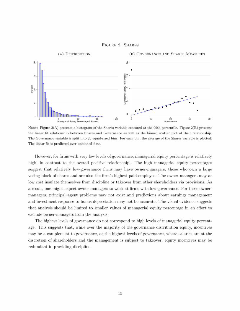
Figure 2: Shares
(a) Distribution
05
1015
20P
erce
nt
0 5 10 15 20Managerial Equity Percentage / Shares
(b) Governance and Shares Measures
05
1015
20M
anag
eria
l Equ
ity P
erce
ntag
e
0 5 10 15 20Governance
Notes: Figure 2(A) presents a histogram of the Shares variable censored at the 99th percentile. Figure 2(B) presents
the linear fit relationship between Shares and Governance as well as the binned scatter plot of their relationship.
The Governance variable is split into 20 equal-sized bins. For each bin, the average of the Shares variable is plotted.
The linear fit is predicted over unbinned data.
However, for firms with very low levels of governance, managerial equity percentage is relatively
high, in contrast to the overall positive relationship. The high managerial equity percentages
suggest that relatively low-governance firms may have owner-managers, those who own a large
voting block of shares and are also the firm’s highest-paid employee. The owner-managers may at
low cost insulate themselves from discipline or takeover from other shareholders via provisions. As
a result, one might expect owner-managers to work at firms with low governance. For these owner-
managers, principal–agent problems may not exist and predictions about earnings management
and investment response to bonus depreciation may not be accurate. The visual evidence suggests
that analysis should be limited to smaller values of managerial equity percentage in an effort to
exclude owner-managers from the analysis.
The highest levels of governance do not correspond to high levels of managerial equity percent-
age. This suggests that, while over the majority of the governance distribution equity, incentives
may be a complement to governance, at the highest levels of governance, where salaries are at the
discretion of shareholders and the management is subject to takeover, equity incentives may be
redundant in providing discipline.
15

Figure 3: Bonus Percentage
(a) Bonus Rates
For Qualifying Assets PurchasedBonus
After Before
09/10/2001 05/06/2003 30%
05/05/2003 01/01/2005 50%
12/31/2004 01/01/2008 0%
12/31/2007 09/09/2010 50%
09/08/2010 01/01/2010 100%
12/31/2011 01/01/2013 50%
(b) Over Time
020
4060
8010
02000 2002 2004 2006 2008 2010 2012
4.3 Z Tax Term
Investment tax policy during this period affected only the present value of tax depreciation al-
lowances, which I will label the “Z Tax Term.”
zt = bt + (1− bt)∞∑i=1
di(1 + r)i
where zt is the present value of tax depreciation allowances on $1 of investment. It is composed of
MACRS statutory depreciation allowances di and bonus depreciation bt.
The Z Tax Term varies both over time and across different types of assets. Variation over time
and within asset types is driven by “bonus depreciation” legislation.28 The policy generally applies
to all property with MACRS depreciation schedules of less than 20 years. Table 1 and Figure 5
display the bonus depreciation rates during the years 2000 to 2012. Variation in the Z Tax Term
across asset types is driven by differences in tax depreciation rates and recovery periods for different
types of capital. 29
Ideally, firm-level investment data by asset type for each year would be available and a firm-
specific weighted tax depreciation rate and Z Tax Term could be constructed. Unfortunately, firm-
28Items of legislation that include bonus depreciation and their effect on the level of bonus depreciation are detailedin Appendix C.
29IRS Publication 946 details how different types of assets may be depreciated. Assets may be depreciated usingeither the straight line method or the double declining balance method. Within each method, a recovery time periodof 5 through 35 years may be applied. Generally, investment assets that have a longer service life must be recoveredover a longer time period. Longer recovery results in lower present value of tax depreciation allowances. Both thesystem and length of recovery are specified for each type of investment in the IRS publication. For an extendeddiscussion of the MACRS, see House and Shapiro (2008).
16
level data on investment by asset types are not available. In lieu of micro-level tax depreciation
rates, I follow Cummins et al. (1994) and Desai and Goolsbee (2004) and construct industry-level
present value tax depreciation rates using the Capital Flows table from the Bureau of Economics
Analysis, which records industry-level investment by asset types.30
To construct industry-level rates, I (1) construct present value tax depreciation rates for each
asset type in the BEA table. (2) For each industry, I weight the asset-level depreciation rates by the
amount of investment made by each asset category for each industry. The industry-level BEA rates
are matched to firms using the NAICS classification system. The industry-level tax depreciation
rates are constructed only for equipment.31 Once the present values of tax depreciation allowances
are constructed at the industry-level, they are combined with bonus depreciation rates over time
and the statutory tax rate to form the Z Tax Term.
For interpretability, I scale the Z Tax Term by the change in the present value of tax depreci-
ation allowances when bonus depreciation varies from 0% to 100% for the firm with average-lived
investment assets. As a result of this scaling, the coefficient on the Z Tax Term in regression can be
interpreted as the increase in It/Kt−1 for the average firm when the bonus goes from 0% to 100%.
4.4 Investment and Control Variables
The dependent variable in all regressions is the investment during the current period scaled by the
stock of capital in place at the beginning of the period. This ratio is measured using Compustat
data,
ItKt−1
=capxt
ppentt−1
where capx is capital expenditures and ppent is property, plant, and equipment.
In all investment regressions, I control for marginal Q. Additional possible determinants of
investment, a measure of cash flows and a measure of financial distress, are included in select
regressions. Appendix B details the construction of these variables. Following Desai and Gooslbee
(2004) and others, I winsorize the investment, marginal Q, and control variables at the 1st and
99th percentiles to minimize the effects of misreported data.
30The BEA classifies investment into 51 categories; 28 are equipment and 23 are structures. Equipment categoriesinclude Computers and Peripheral Equipment, Mining and Oilfield Machinery, and Autos. Structures categoriesinclude Industrial Buildings, Residential Buildings, and Farm Nonresidential Structures. The BEA classifies firmsinto 123 industries which can be matched to 3-digit NAICS codes.
31Bonus depreciation cannot be applied the purchase of structures. A separate Z Tax Term can be constructed forstructures, however, because the term does not vary within industries over time, when firm and year fixed effects areincluded in regression, a coefficient on the structures tax term cannot be separately identified.
Because bonus depreciation cannot be applied to the purchase of structures, the percentage of capital investmentin structures as a fraction of total investment may also influence stock prices reactions to the bonus depreciationpolicy. Firms that invest a larger percentage in structures should have smaller abnormal returns after the extensionof the policy. The event study results are unchanged when industry-level structures tax rates are included.
17

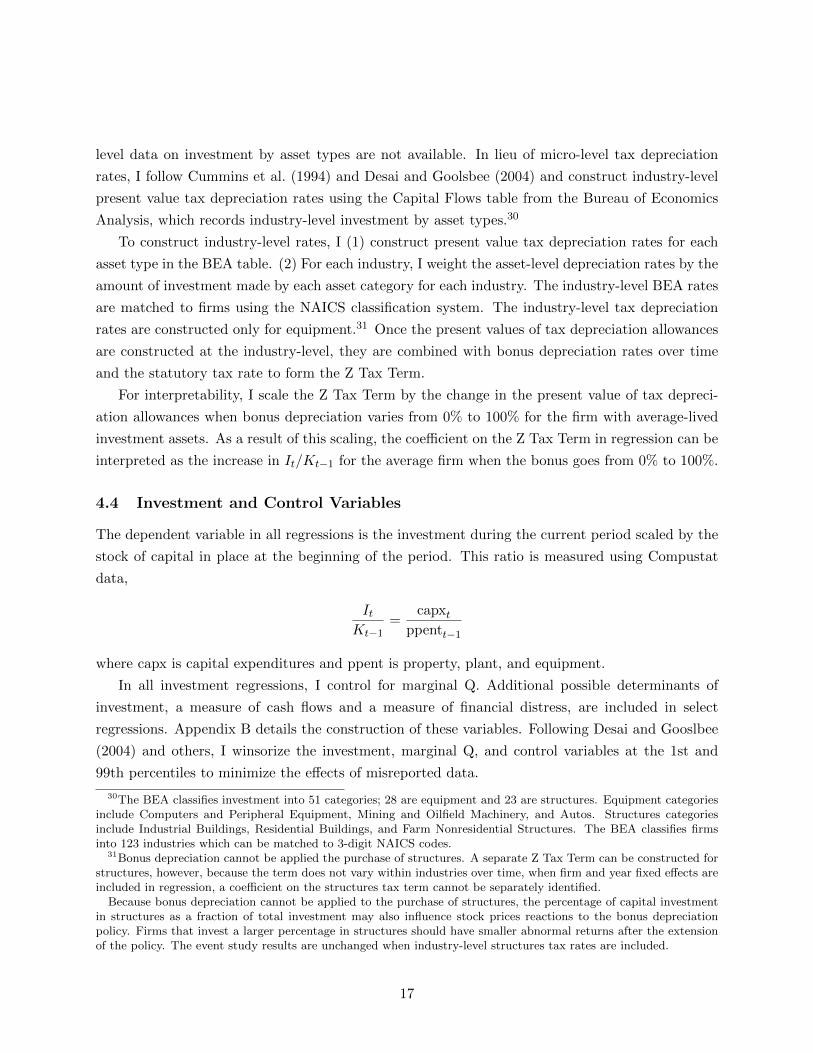
4.5 Descriptive Statistics
Table 1 presents descriptive statistics on capital expenditure, the Z tax term, cash flow, marginal
Q, cash flows and the financial constraint measure, both for the full sample and then separately
for governance sample (those firms for which governance and managerial equity data are available).
Table 1 also presents descriptive statistics for the measures of corporate governance, Governance,
Entrenchment, and Shares.
Firm-level data on investment, cash flows, financial constraints, and marginal Q are similar
to the prior literature. The governance sample is composed of more mature firms. Consistent
with their maturity, firms in the governance sample are less financially constrained, have larger
cash flows, invest less relative to their stock of capital, and have lower values of marginal Q than
the full sample. The average investment as a fraction of existing capital observed is 0.255 in the
governance sample, meaning that in each year the average firm invests an amount approximately
equal to one-quarter of their existing capital stock.
The average firm in the governance sample has a Governance score of 9, meaning that the
average firm has 9 fewer provisions protecting managers from shareholder discipline than the firm
with the maximum number of these such provisions. The average value of Entrenchment is 3.758,
meaning that the average firm has approximately 2.24 provisions protecting management from
shareholders.
The average value of Shares is 3.66% and the distribution is skewed to the left; the modal
managerial equity percentage is only 1.3%. 58% of top executives hold more than 1%, 27 hold
more than 3%, and only 17.9 hold more than 5%.
5 Estimation Strategy
The estimating equation implied by the model in Section 3 is
IitKi,t−1
= β0 + β1zTjt+β2Git + β3Gitτz
Tjt + β4
[λitpit− 1
]+ εit.
The Z Tax Term varies both across industries, due to MACRS regulations, and over time, due
to bonus depreciation. With firm and year fixed effects, identification of the β1 coefficient comes
from how changes in bonus depreciation differentially affect industries. Industries that invest in
longer-lived equipment benefit more from the policy than industries that invest in equipment that
depreciates quickly for tax purposes.
The Governance variable varies across firms and over time. With firm fixed effects, the β2
parameter is identified off of within-firm variation in the Governance variable. This variable is
potentially endogenous to within firm variation in investment behavior. Shareholders could con-
ceivably choose to significantly increase governance when the firm increases investment behavior.
18
Table 1: Descriptive Statistics Years 2000-2010
Median Mean Std. Dev. Obs.Full Sample
Cap Exp / Prop Plant Equip 0.197 0.357 0.544 76,497Z Tax Term 0.487 0.483 0.036 92,311Q/(1-τ) 2.130 4.482 10.074 93,823Cash Flow / PPE 0.205 -1.403 8.295 71,659HP Financial Constraint -4.244 -4.161 1.946 80,013
Governance Sample
Cap Exp / Prop Plant Equip 0.185 0.255 0.274 11,606Z Tax Term 0.488 0.484 0.031 13,196Q/(1-τ) 2.242 2.873 2.123 12,113Cash Flow / PPE 0.409 0.599 2.572 11,314K-Z Financial Constraint -6.172 -6.071 1.077 12,478
Governance, Equity
Governance 9 8.966 2.557 15,422Bebchuk 4 3.758 1.277 15,422
Shares 1.302 3.661 6.726 19,976
Note: The investment and tax variables are provided for both the full sample and for the governance sample. The
governance sample are firms for which both governance and managerial equity incentive data are available.
19
However, because the parameter of interest is constructed as a ratio of β1 and β3, any impact of
within-firm variation of investment on governance should not compromise testing of the primary
empirical hypothesis. The crucial assumption is not that the level of governance is exogenous to
investment, but that the level of governance is exogenous to investment response to bonus depre-
ciation, which is a plausible assumption.
Because the Governance variable is relatively stable within firms over time (see Gompers et
al. (2003)), identification of the β3 parameter comes from variation in the mean governance level
and variation across industries in how much bonus depreciation decreases the present value cost
of investment.32 The variable is larger when bonus depreciation hits firms with high levels of
governance.
A potential threat to identification would arise if firms with low-governance levels invested pri-
marily in long-lived assets, which would increase the impact of bonus depreciation on investment.
If this were the case, then estimation would inaccurately attribute investment response to low levels
of governance when only differential impacts of the tax policy across industries are driving invest-
ment behavior. One observation that mitigates this threat is that there appears to be significant
variation in Governance levels within industries. As a result, there exists within industry variation
in the interaction term. In Appendix I, I add industry-year fixed effects to baseline regression to
further alleviate this concern. With industry-year fixed effects, the β3 coefficient is identified from
within-industry variation in the interaction term, coming only from across firm differences in Gov-
ernance levels. The drawback of using industry-year fixed effects is that the β1 coefficient can no
longer be estimated. However, the sign and magnitude of the interaction coefficient are similar to
baseline results, suggesting that baseline results are not driven by a correlation of low governance
and long-lived assets.
6 Investment Response to Bonus Depreciation
6.1 Visual Analysis of Investment Responsiveness to Bonus Depreciation
Figure 4 presents the effect of bonus depreciation on investment for firms with different level of
governance. In all four panels, firms are split according to Governance levels. Firms with Gover-
nance levels more than 1 standard deviation below the mean are classified as “Low Governance;”
others are classified as “High Governance.” Panels (A) and (B) show the impact of the 2001 and
2008 bonus episodes on firms with generous MACRS statutory depreciation allowances (di) – those
firms which should be unaffected by the policy. Panels (C) and (D) limit the analysis to firms with
high di – the firms “treated” by the policy.
32Regressions that use mean Governance levels are presented in Appendix E. Coefficients on the interaction pa-rameter have magnitudes similar to baseline results, confirming that identification of β3 is not driven by within-firmchanges in Governance.
20

Figure 4: Investment Response to Bonus Depreciation by Governance Levels
(a) Bonus 1: “Untreated” Firms
.25
.3.3
5.4
.45
Inve
stm
ent P
erce
nt
1998 2004
Low Governance FirmsHigh Governance Firms
(b) Bonus 2: “Untreated Firms”
.2.2
5.3
.35
.4In
vest
men
t Per
cent
2005 2011
Low Governance FirmsHigh Governance Firms
(c) Bonus 1:“Treated Firms”
.25
.3.3
5.4
.45
Inve
stm
ent P
erce
nt
1998 2004
Low Governance FirmsHigh Governance Firms
(d) Bonus 2: “Treated Frims”
.2.2
5.3
.35
.4In
vest
men
t Per
cent
2005 2011
Low Governance FirmsHigh Governance Firms
Notes: Figures 4(A) - 4(D) plots the mean investment percent for groups sorted by their governance levels and
present values of statutory depreciation allowances. (A) and (B) show “untreated” firms – those with above median
depreciation allowances. (C) and (D) show “treated firms” – those with below median depreciation allowances. Panels
(A) and (C) examine years around the first bonus episode (2001-2004). Panels (B) and (D) examine years during the
second bonus episode (2005-2011). In all panels, firms are split by governance levels. Low Governance firms are with
G Indices more than one standard deviation below the mean. High Governance firms have governance scores higher
than one standard deviation above the mean. Group averages are derived through the following procedure: cross-
sectional regression of investment percent on controls for marginal Q, cash flow, and the HP Index are run separately
for each year. Residual group means are then calculated for the Low and High Governance groups. Finally, to
normalize investment behavior prior to policy implementation group means are equalized in years 1999-2000 and
2006-2007 to ease the comparison of trends. All means are count weighted.
21
Figure 4 presents compelling visual evidence that investment is less responsive to bonus depre-
ciation for firms with high levels of governance. This pattern of response is consistent with the
hypothesis that corporate governance induces earnings management behavior. For the Untreated
group, when the policy is enacted in 2001 and again in 2008, the behaviors of the Governance groups
are not differentially affected. But for the treated firms, the response is heavily concentrated among
the least governed firms. The intuitive explanation for this unresponsiveness by High Governance
firms is that the managers of these firms are highly incentivized to focus on maximizing accounting
earnings, the most salient measure of corporate performance. Because accounting earnings are
unaffected by bonus depreciation, firms with high levels of governance are unresponsive.
6.2 Replicating Previous Literature
The first four columns of Table 2 replicate prior empirical studies of bonus depreciation both for all
Compustat firms and for the smaller Governance sample. Specification (1) regresses It/Kt−1 on the
Z Tax Term and marginal Q, and includes year and firm fixed effects. Specification (2) repeats the
regression from the first specification, but includes cash flow and financial distress controls. The Z
Tax Term coefficient is interpreted as the increase in It/Kt−1 that results from an increase in bonus
depreciation from 0 to 100% for the firm with average MACRS statutory depreciation rates.
Without additional controls for investment, a 100% increase in bonus depreciation is associated
with an increase in It/Kt−1 of 0.04, approximately an 11% increase in investment as a percentage
of installed capital. When additional controls are added to the regression, the effect of a 100%
increase in bonus depreciation is approximately a 4% increase relative to the mean investment
level, suggesting that the controls are correlated with the tax policy. Specification (2) results are
in line with the bonus depreciation literature and demonstrate the empirical puzzle, addressed by
House and Shapiro (2008) and Edgerton (2012), that investment is not strongly responsive to bonus
depreciation, despite the temporary nature of the policy and the policy’s potential to significantly
decrease the net present value costs of investment.
Specifications (3) and (4) repeat the regressions of specifications (1) and (2), but limit the
sample to firms for which governance data was available. Specification (4) shows that the effect of
moving from 0 to 100% bonus depreciation has an impact on investment that is very similar for
the full sample and for the governance sub-sample.
6.3 Baseline Results
Baseline results presented in Specifications (5) and (6) of Table 2 show a strong heterogeneous
response across different levels of governance. Consistent with the governance–earnings manage-
ment hypothesis, firms with high levels of governance are less responsive to bonus depreciation.
Specification (5) fits the linear estimating equation implied by the theoretical model to the data;
22
specification (6) adds additional controls for cash flows and financial distress. In these regressions,
the Z Tax Term can now be interpreted as the effect of increasing the bonus depreciation from 0
to 100% for the firm with the average MACRS statutory tax depreciation rates and a Governance
score of 0. The regression predicts that for the hypothetical zero governance firm , increasing
bonus depreciation from 0 to 100% results in an increase of It/Kt−1 by 0.177 or an increase by
69% increase relative to mean investment levels. This effect is large and can viewed as how firms
would respond to the policy if they placed the minimal amount of focus on accounting earnings.
This effect is nearly 10 times as large as the effect for the firm with the mean level of governance.
The investment response to bonus depreciation decreases as the level of governance increases.
The coefficient on the interaction term in (5) and (6) is interpreted as the change in the Z Tax
Term coefficient resulting from a one standard deviation increase in Governance relative to the
mean level. Each one standard deviation increase in Governance decreases the It/Kt−1 response by
0.046 (approximately 27%). The γG presented in Table 2 is the percentage decrease in investment
response to bonus depreciation that results from a one standard deviation increase in governance.
γG is approximately 0.27 in specification (6), meaning that a one standard deviation increase in
governance makes firms 27% less responsive to bonus depreciation. These results strongly support
the theoretical hypothesis that more strongly governed managers focus their attention on accounting
earnings. Strongly governed firms are less responsive to bonus depreciation and demonstrate more
earnings management behavior. 33
Marginal effects of bonus depreciation on investment at different levels of Governance are pre-
sented in Table 3. As a result of bonus depreciation going from 0 to 100%, investment percentage
increases by 0.097 or 28% compared to average levels for firms with Governance level two standard
deviations below the mean level. For firms with Governance levels one standard deviation below
the mean, bonus depreciation increases investment percentage by 16%. Investment responses for
firms at the mean level of Governance and with Governance one standard deviation higher than
the mean are not statistically different from zero.
Note that the estimates suggest that investment responds negatively to bonus depreciation for
firms with very high levels of governance. This result is not consistent with the behavior of eco-
nomically rational actors or with the tax policy itself. Investment response to the policy should be
bounded below by zero, because not only do firms not have to respond to bonus depreciation, but
they can also choose not to take bonus depreciation and, instead, write off investment using statu-
tory MACRS schedules.34 Therefore, there must be other factors driving the negative estimated
33Gompers et al. (2003) broke down the “G Index” into 5 categories: (1) tactics for delaying hostile takeovers, (2)voting rights, (3) director/officer protection, (4) other takeover defenses, and (5) state laws. The baseline regressionis presented separately for each category and then for all the categories together in Appendix G. The results indicatethat no one category fully determines the heterogeneous investment response to bonus depreciation, suggesting thatthe Governance variable is an adequate measure of the overall level of governance faced by firm managers.
34Knittle (2007) noted that only 55–63% of corporate investment actually claimed bonus depreciation during the2002 to 2004 episode. The paper suggested that the low take-up rate was a product of three factors: the temporary
23

Table 2: Baseline Analysis, Governance Index
Dependent Variable Capital Expenditure / Property Plant Equipment
Specification (1) (2) (3) (4) (5) (6)
Z Tax Term 0.040*** 0.015 0.027* 0.013 0.177*** 0.172***(0.010) (0.010) (0.015) (0.014) (0.033) (0.033)
Governance 0.357*** 0.396***(0.056) (0.059)
Gov x Z TT -0.043*** -0.046***(0.008) (0.008)
γG 0.244*** 0.268***(0.033) (0.034)
Firms 12,932 12,047 1,944 1,915 1,944 1,915Firm x Years 78,506 71,773 14,261 13,531 14,261 13,531
Notes: Specifications (1) through (4) present coefficients from regressions of the form
IitKi,t−1
= β0 + β1zTit + β2
λitpit
+ εit.
Specifications (5) and (6) include governance measures and present regressions of the form
IitKi,t−1
= β0 + β1τzTit + β2Git + β3Gitτz
Tit + β4
λitpit
+ εit.
Specifications (2), (4), and (6) include additional controls for financial distress and cash flows. All specifications
include firm and year fixed effects and marginal Q. Standard errors are clustered at the firm level and are robust to
heteroskedasticity. *** indicates statistical significance at the 1% level, ** at 5%, and * at 10%.
Table 3: Investment Response Marginal Effects
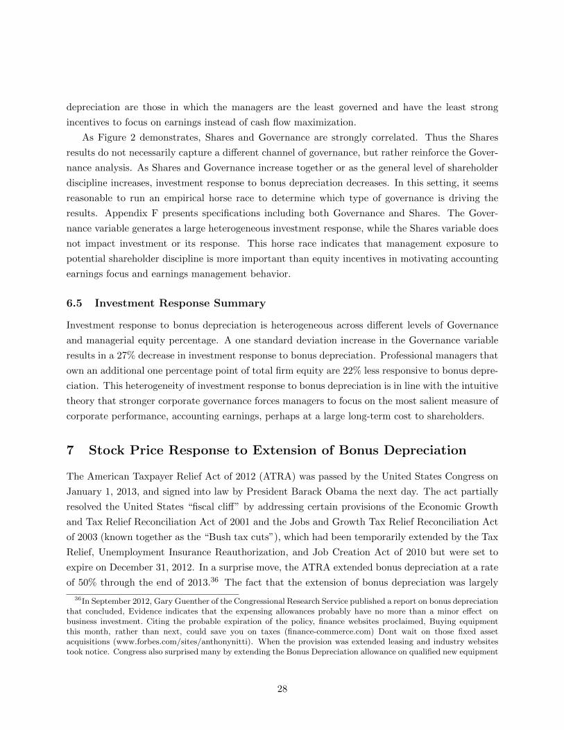
Governance Level -2 -1 0 +1 + 2Std. From Mean
d(It/Kt−1) 0.103*** 0.057*** 0.011 -0.035 -0.082***/d Z TT (0.024) (0.019) (0.016) (0.018) (0.023)
% of mean (It/Kt−1) 28% 16% 3.1% -9.8% -23%
Notes: Table 3 provides marginal effects estimates of the change in It/Kt−1 from an increase in bonus depreciation
from 0 to 100% for firms at different levels of Governance. Marginal effects are provided for firms with mean level
Governance and firms with Governance ± 1 and ± 2 standard deviations from the mean. Marginal effects are derived
from the regression presented in specification (6) of Table 3. *** indicates statistical significance at the 1% level.
24
response.
One possible explanation is that this estimation strategy may not sufficiently control for general
equilibrium effects of the policy. As noted by Goolsbee (1998), investment tax incentives can
affect the purchase price of capital, thereby depressing investment response to the policy. In the
theoretical model, the price of investment goods should be reflected in marginal Q. Marginal Q
may not sufficiently control for these general equilibrium effects. For the strongly governed firms,
the tax policy does not increase the tax benefit of investment because managers care only to
maximize accounting earnings. Strongly governed firms may, however, experience price increases
in investment goods as a result of the policy. For strongly governed firms, there is no upside to
the policy, only downside. Because governance varies significantly within industries, price increases
in investment goods should not be a function of the governance level and should not effect the
estimation of heterogeneous response to the policy or the relationship between corporate governance
and earnings management behavior.35
However, due to the accounting treatment of the cost of investment, these general equilibrium
effects may be unable to explain the negative responsiveness phenomena. Recall that the purchase
price of new capital does not affect accounting earnings; the cost of new investment is subtracted
from accounting earnings only as the newly installed capital depreciates for book purposes. Thus,
firms with high levels of governance that place a large weight on accounting earnings should not
benefit from the tax policy nor be as significantly affected by potential investment price shocks as
firms that place less emphasis on accounting earnings.
Another possibility is that the severity of the 2008 and 2009 recession is not sufficiently captured
by the model. The model does not account for supply-side financing constraints, which were
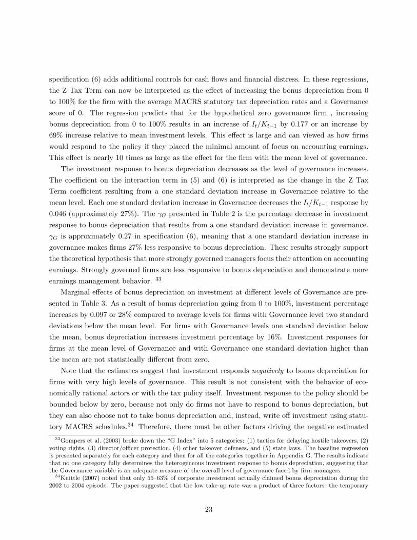
significant during the height of the recession. To test this explanation, I estimate specification (6)
from Table 2 using only data prior to year 2008. Marginal effects from this temporally adjusted
regression are presented in Table 4. During years prior to 2008, investment was more responsive to
the tax policy. Firms with mean-level Governance increased investment as a percentage of installed
capital by nearly 10%. Furthermore, the investment response of the most strongly governed firms
was not statistically different from zero, suggesting that financing constraints, which were the
largest when bonus depreciation was at its highest level (during the sample period), may be driving
the negative responsiveness among the most highly governed firms.
Overall, the baseline analysis supports the hypothesis that corporate governance induces earn-
ings management behavior. Consistent with the hypothesis, more strongly governed firms are less
responsive to bonus depreciation. Using the heterogeneous response to the policy, I estimate that
nature of the policy, significant tax losses which mitigated the policy’s impact, and the non-conformity of some statetax systems to the federal policy.
35While Goolsbee (1998) found that investment prices increase 3.5 to 7% when investment tax credits are increasedby 10%, House and Shapiro (2008) found that investment prices were unresponsive to bonus depreciation in 2001through 2004.
25
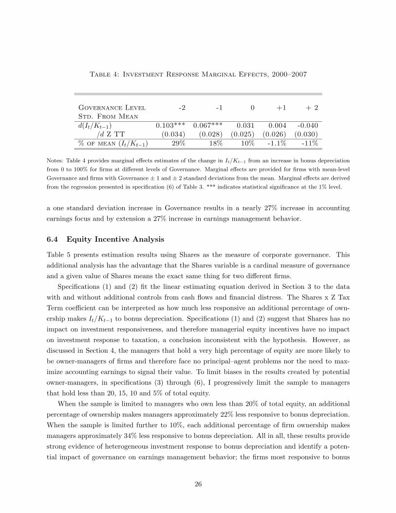
Table 4: Investment Response Marginal Effects, 2000–2007
Governance Level -2 -1 0 +1 + 2Std. From Mean
d(It/Kt−1) 0.103*** 0.067*** 0.031 0.004 -0.040/d Z TT (0.034) (0.028) (0.025) (0.026) (0.030)
% of mean (It/Kt−1) 29% 18% 10% -1.1% -11%
Notes: Table 4 provides marginal effects estimates of the change in It/Kt−1 from an increase in bonus depreciation
from 0 to 100% for firms at different levels of Governance. Marginal effects are provided for firms with mean-level
Governance and firms with Governance ± 1 and ± 2 standard deviations from the mean. Marginal effects are derived
from the regression presented in specification (6) of Table 3. *** indicates statistical significance at the 1% level.
a one standard deviation increase in Governance results in a nearly 27% increase in accounting
earnings focus and by extension a 27% increase in earnings management behavior.
6.4 Equity Incentive Analysis
Table 5 presents estimation results using Shares as the measure of corporate governance. This
additional analysis has the advantage that the Shares variable is a cardinal measure of governance
and a given value of Shares means the exact same thing for two different firms.
Specifications (1) and (2) fit the linear estimating equation derived in Section 3 to the data
with and without additional controls from cash flows and financial distress. The Shares x Z Tax
Term coefficient can be interpreted as how much less responsive an additional percentage of own-
ership makes It/Kt−1 to bonus depreciation. Specifications (1) and (2) suggest that Shares has no
impact on investment responsiveness, and therefore managerial equity incentives have no impact
on investment response to taxation, a conclusion inconsistent with the hypothesis. However, as
discussed in Section 4, the managers that hold a very high percentage of equity are more likely to
be owner-managers of firms and therefore face no principal–agent problems nor the need to max-
imize accounting earnings to signal their value. To limit biases in the results created by potential
owner-managers, in specifications (3) through (6), I progressively limit the sample to managers
that hold less than 20, 15, 10 and 5% of total equity.
When the sample is limited to managers who own less than 20% of total equity, an additional
percentage of ownership makes managers approximately 22% less responsive to bonus depreciation.
When the sample is limited further to 10%, each additional percentage of firm ownership makes
managers approximately 34% less responsive to bonus depreciation. All in all, these results provide
strong evidence of heterogeneous investment response to bonus depreciation and identify a poten-
tial impact of governance on earnings management behavior; the firms most responsive to bonus
26
Table 5: Managerial Equity Percentage Analysis
Dependent Variable Capital Expenditure / Property Plant Equipment
Specification (1) (2) (3) (4) (5) (6)Shares Restriction < 20% < 15% < 10% < 5%
Z Tax Term 0.032** 0.021 0.033** 0.025 0.028* 0.029(0.016) (0.016) (0.016) (0.016) (0.017) (0.019)
Shares 0.009 0.014* 0.053*** 0.045** 0.068*** 0.109**(0.008) (0.007) (0.017) (0.018) (0.025) (0.047)
Shares x Z TT -0.001 -0.002* -0.007*** -0.006** -0.009** -0.015**(0.001) (0.001) (0.003) (0.003) (0.004) (0.007)
γS 0.041 0.090 0.222* 0.251 0.338* 0.520*(0.035) (0.075) (0.120) (0.157) (0.195) (0.300)
Firms 2,348 2,300 2,263 2,234 2,189 2,080Firm x Years 17,352 16,422 15,807 15,491 14,935 13,545
Notes: Table 5 presents regressions of the form
IitKi,t−1
= β0 + β1τzTit + β2Sit + β3Sitτz
Tit + β4
λitpit
+ εit.
Specifications (2) through (6) include additional controls for financial distress and cash flows. All specifications
include firm and year fixed effects and marginal Q. Standard errors are clustered at the firm level and are robust to
heteroskedasticity. *** indicates statistical significance at the 1% level, ** at 5%, and * at 10%.
27
depreciation are those in which the managers are the least governed and have the least strong
incentives to focus on earnings instead of cash flow maximization.
As Figure 2 demonstrates, Shares and Governance are strongly correlated. Thus the Shares
results do not necessarily capture a different channel of governance, but rather reinforce the Gover-
nance analysis. As Shares and Governance increase together or as the general level of shareholder
discipline increases, investment response to bonus depreciation decreases. In this setting, it seems
reasonable to run an empirical horse race to determine which type of governance is driving the
results. Appendix F presents specifications including both Governance and Shares. The Gover-
nance variable generates a large heterogeneous investment response, while the Shares variable does
not impact investment or its response. This horse race indicates that management exposure to
potential shareholder discipline is more important than equity incentives in motivating accounting
earnings focus and earnings management behavior.
6.5 Investment Response Summary
Investment response to bonus depreciation is heterogeneous across different levels of Governance
and managerial equity percentage. A one standard deviation increase in the Governance variable
results in a 27% decrease in investment response to bonus depreciation. Professional managers that
own an additional one percentage point of total firm equity are 22% less responsive to bonus depre-
ciation. This heterogeneity of investment response to bonus depreciation is in line with the intuitive
theory that stronger corporate governance forces managers to focus on the most salient measure of
corporate performance, accounting earnings, perhaps at a large long-term cost to shareholders.
7 Stock Price Response to Extension of Bonus Depreciation
The American Taxpayer Relief Act of 2012 (ATRA) was passed by the United States Congress on
January 1, 2013, and signed into law by President Barack Obama the next day. The act partially
resolved the United States “fiscal cliff” by addressing certain provisions of the Economic Growth
and Tax Relief Reconciliation Act of 2001 and the Jobs and Growth Tax Relief Reconciliation Act
of 2003 (known together as the “Bush tax cuts”), which had been temporarily extended by the Tax
Relief, Unemployment Insurance Reauthorization, and Job Creation Act of 2010 but were set to
expire on December 31, 2012. In a surprise move, the ATRA extended bonus depreciation at a rate
of 50% through the end of 2013.36 The fact that the extension of bonus depreciation was largely
36In September 2012, Gary Guenther of the Congressional Research Service published a report on bonus depreciationthat concluded, Evidence indicates that the expensing allowances probably have no more than a minor effect onbusiness investment. Citing the probable expiration of the policy, finance websites proclaimed, Buying equipmentthis month, rather than next, could save you on taxes (finance-commerce.com) Dont wait on those fixed assetacquisitions (www.forbes.com/sites/anthonynitti). When the provision was extended leasing and industry websitestook notice. Congress also surprised many by extending the Bonus Depreciation allowance on qualified new equipment
28

unexpected creates a natural experiment that can be used to corroborate investment results that
indicate strong corporate governance induces earnings management behavior.
To examine the impact of the surprise extension of bonus depreciation, I rely on event study
methodology. To use the ATRA event study to examine the impact of governance and earnings
management, I empirically address two questions. First: are abnormal returns higher for firms
that, on average, invest in longer lived equipment assets, (those with on-average slower statutory
depreciation rates) i.e. those who stand to gain the most from the extension of bonus depreciation?
Second: are abnormal returns to the policy relatively higher for firms with weaker corporate gov-
ernance? If both questions are answered in the affirmative, then the ATRA event study provides
additional support that governance encourages earnings management behavior. In light of the in-
vestment response to bonus depreciation, the answers to these questions also address whether, at
least in the context of bonus depreciation, the market values low governance, which allows managers
to respond to the policy.
7.1 Cumulative Abnormal Returns
In order to perform an event study, abnormal returns are computed for each firms for the days
after the event occurs and are multiplicatively compiled to produce cumulative abnormal returns
that describe by how many percentage points a stock over- or under-performs its expected return
t days after the event. I rely on the Fama-French Value Weighted Three Factor Model (Fama
and French (1992), Fama and French (1993)) to generate expected returns and then compare this
prediction against the actual observed stock returns to generate the abnormal and cumulative
abnormal returns.37 The cumulative abnormal return, CARit, will be the dependent variable in
the fiscal cliff event study. It is defined as the Cumulative Abnormal Return for firm i, t days after
(www.teqlease.com/2013/01/08/the-fiscal-cliff-deal-saves-bonus-depreciation/) One major surprise was a generousrenewal of Sec. 179 and bonus depreciation rules that have allowed high-income farm operations to shelter sizableincomes in recent years. (http://www.dtnprogressivefarmer.com). The surprise is confirmed empirically. See Figures9 and 10.
37More precisely: using daily stock data from CRSP for the month prior to the passage of the ATRA, I regressthe return for each firm above the risk free rate, Rit −Rft, on three factors: (1) the market return over the risk-freerate Rmt − Rft, (2) the value-weighted return on small firms over the value-weighted return on large firms SMB,and (3) the value-weighted return on high book-to-market value firms minus the return on low book-to-market valuefirms HML. The regressions produce coefficients β, γ, and δ for each firm. I then use these coefficients to predicteach individual firm’s performance after the passage of the ATRA. How much the firm over or underperforms thisprediction during a trading day is the firm’s abnormal performance, a;
ait = [Rit −Rft]︸ ︷︷ ︸actual
− [β̂i(Rmt −Rft) + γ̂i(SMB) + δ̂i(HML)]︸ ︷︷ ︸estimated
.
Once the abnormal returns have been estimated, I construct Cumulative Abnormal Returns for each firm t daysafter the passage of ATRA 2012, CARit. The multiplicative cumulative abnormal returns are often referred to asBuy-and-Hold Abnormal Returns or BHARS. In constructing traditional CARS, one simply adds abnormal returnstogether. This procedure, however, is not appropriate when abnormal returns are defined in percentage points aboveor below predicted returns.
29
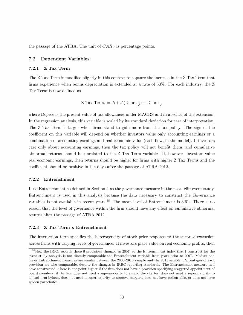
the passage of the ATRA. The unit of CARit is percentage points.
7.2 Dependent Variables
7.2.1 Z Tax Term
The Z Tax Term is modified slightly in this context to capture the increase in the Z Tax Term that
firms experience when bonus depreciation is extended at a rate of 50%. For each industry, the Z
Tax Term is now defined as
Z Tax Termj = .5 + .5(Deprecj)−Deprecj
where Deprec is the present value of tax allowances under MACRS and in absence of the extension.
In the regression analysis, this variable is scaled by its standard deviation for ease of interpretation.
The Z Tax Term is larger when firms stand to gain more from the tax policy. The sign of the
coefficient on this variable will depend on whether investors value only accounting earnings or a
combination of accounting earnings and real economic value (cash flow, in the model). If investors
care only about accounting earnings, then the tax policy will not benefit them, and cumulative
abnormal returns should be unrelated to the Z Tax Term variable. If, however, investors value
real economic earnings, then returns should be higher for firms with higher Z Tax Terms and the
coefficient should be positive in the days after the passage of ATRA 2012.
7.2.2 Entrenchment
I use Entrenchment as defined in Section 4 as the governance measure in the fiscal cliff event study.
Entrenchment is used in this analysis because the data necessary to construct the Governance
variables is not available in recent years.38 The mean level of Entrenchment is 3.61. There is no
reason that the level of governance within the firm should have any effect on cumulative abnormal
returns after the passage of ATRA 2012.
7.2.3 Z Tax Term x Entrenchment
The interaction term specifies the heterogeneity of stock price response to the surprise extension
across firms with varying levels of governance. If investors place value on real economic profits, then
38How the IRRC records these 6 provisions changed in 2007, so the Entrenchment index that I construct for theevent study analysis is not directly comparable the Entrenchment variable from years prior to 2007. Median andmean Entrenchment measures are similar between the 2000–2010 sample and the 2011 sample. Percentages of eachprovision are also comparable, despite the changes in IRRC reporting standards. The Entrenchment measure as Ihave constructed it here is one point higher if the firm does not have a provision specifying staggered appointment ofboard members, if the firm does not need a supermajority to amend the charter, does not need a supermajority toamend firm bylaws, does not need a supermajority to approve mergers, does not have poison pills, or does not havegolden parachutes.
30

they should value not only the policy itself, but also low governance levels, which allow managers
to respond to the policy. Again, the sign on the coefficient depends on whether or not investors
value only accounting earnings or a combination of accounting earnings and cash flow. If investors
value only accounting earnings, then the coefficient on the interaction term should be zero. If,
however, investors place some value on cash flows, then investors would prefer managers that are
able to respond to the policy, i.e., those in firms with low governance levels. If this is the case, then
investors value high Z Tax Terms and low Entrenchment, and cumulative abnormal returns should
be negatively related to the interaction variable.
7.3 Event Study Results
Table 7 presents the event study results.39 Each column represents a separate regression as the
dependent variable evolves from cumulative abnormal returns 1 day after passage ATRA 2012 to 6
days after the passage of ATRA 2012. The dependent CAR variable is regressed on the governance
measure, Entrenchment, the present value of statutory tax depreciation allowances, Deprec, and
the interaction of the two variables.40 Looking across the table from left to right, the reader can
see how the effect of governance, potential benefit from the extension of bonus depreciation, and
the interaction of the two are related to cumulative abnormal returns over time.
The event study results suggest that investors value not only bonus depreciation, but also low
levels of governance, which allow firms to respond to the tax policy. The Z Tax Term coefficient is
positive and statistically different from zero 2, 3, and 4 days after the passage of ATRA 2012. These
results indicate that abnormal returns are higher for firms with lower MACRS depreciation rates
– those firms that stand to benefit from the extension from a cash flow perspective. Cumulative
abnormal returns after the passage of ATRA 2012 indicate that investors value bonus depreciation.
The coefficient on the interaction of the Z Tax Term and Entrenchment is negative and statis-
tically different from zero 2, 3, 4, and 5 days after the passage of ATRA 2012, suggesting that for
firms that stand to gain from bonus depreciation, those with low values of governance, are valued
by investors. Consistent with our hypothesis, abnormal returns are the highest for firms that should
respond to bonus depreciation (those with high Z Tax Terms) and for those that do respond to
the policy (those with low governance measures). Taken together, this evidence suggests that, in
the context of bonus depreciation, strong governance, which places managerial focus on accounting
earnings and limits the firms ability to respond to the extension of the policy, is value decreas-
ing. An alternative way to view these results is that investors do not value strong governance, in
39Appendix M presents two placebo event studies. Using the estimated parameters from the Fama French Value-Weighted Three Factor Model, I produce CARs beginning on December 10, 2012, and then again for January 15,2013. No coefficients from either event study are estimated to be statistically different from 0 at the 95% level. Inthe December 10 placebo, the Deprec coefficient does have a positive coefficient different from zero at the 90 percentlevel.
40Cash flows are included in all regressions to control for firms’ ability to respond to bonus depreciation.
31

Table 6: Americian Taxpayer Relief Act 2012 Event Study Results
Dependent Variable CAR1 CAR2 CAR3 CAR4 CAR5 CAR6
Entrenchment -0.049 -0.043 -0.031 -0.095 -0.075 -0.031(0.102) (0.096) (0.118) (0.127) (0.147) (0.176)
Z TT 0.000 0.448** 0.644*** 0.429** 0.361 0.095(0.322) (0.187) (0.168) (0.176) (0.222) (0.292)
Entrenchment x Z TT -0.251 -0.411*** -0.457** -0.465** -0.320 -0.186(0.211) (0.149) (0.183) (0.177) (0.214) (0.248)
Observations 1,189 1,189 1,189 1,189 1,189 1,189
Table 6 presents results for regressions of the form
CARt = β0 + β1 [Entrenchment] + β2 [Deprec Rate] + β3 [Entrenchment X Deprec Rate]
CARt is the cumulative abnormal return t trading days after the American Taxpayer Relief Act of 2012 was signedinto law on January 1, 2013. Controls for cash flow are included in each regression. Standard errors are robust toheteroskedasticity. *** indicates statistical significance at the1 % level, ** at 5%, and * at 10%.
the context of bonus depreciation, because it induces earnings management behavior and limits
response to the tax policy; earnings management behavior is this setting is value decreasing.
I focus on the third column of Table 6 to examine the magnitude of the point estimates. Three
days after the passage of ATRA 2012, a one standard deviation decrease in the present value of Z
Tax Term results in a 0.644 percentage point over-performance. The coefficient on the interaction
term is equal to -0.457. The interpretation of this estimate is that for a firm whose benefit from the
policy is one standard deviation above the mean, a one standard deviation decrease in governance
increases cumulative abnormal return by an additional 0.457 percentage points. These estimates are
consistent with back-of-the envelope calculations that utilize results from the investment response
analysis; details are provided in Appendix K.
Marginal effects of an additional standard deviation Z Tax Term are presented across various
levels of governance in Table 7. When governance levels are low and the firm is responsive to bonus
depreciation (as determined in the investment analysis), the extension of the bonus has a large
impact on abnormal returns. However, when governance measures are high, the effect of the bonus
on abnormal returns is not statistically different from zero. Again, bonus depreciation is valued by
32
Table 7: Cumulative Abnormal Returns Marginal Effects
Governance Level -2 -1 0 +1 + 2Std. From Mean
d(CAR3) 1.558*** 1.101*** 0.644*** 0.187 -0.267/d(Z TT) (0.466) (0.305) (0.181) (0.190) (0.321)
Notes: Table 7 provides marginal effects estimates of the change in cumulative abnormal returns 3 days after the
passage of ATRA 2012 resulting from a one standard deviation increase in depreciation rates. Marginal effects are
provided for firms with mean level Governance and firms with Governance ± 1 and ± 2 standard deviations from
the mean. Marginal effects are derived from the regression presented in column 3 of Table 7. *** indicates statistical
significance at the 1% level.
the market, and the value of the policy is larger among those firms with low levels of governance,
who will potentially be most responsive to the policy.
7.4 Visual Representation of Event Study Results
Figure 5 presents the event study results from Table 7 visually. Each data point represents a
coefficient from a different regression where the CAR dependent variable is changing over time.
The dotted lines represent lower and upper bounds predicted with 95% confidence. From the visual
representation of the regression results, one may observe that the Deprec coefficient is negative
and statistically different from zero 2, 3, and 4 days after the passage of ATRA 2012. Figure
refeventstudy shows that the interaction coefficient is positive and statistically different from zero
2, 3, 4, and 5 days after the passage of ATRA 2012.
One concern with these results in that they are driven by pre-trends and not a product of the
event. To address these concerns, Figures 6 presents CARs that are constructed beginning 5 days
prior to the passage of ATRA 2012. The disadvantage of constructing CARs that begin prior to
the event is that additional variation unrelated to the event is introduced.
Cumulative abnormal returns are close to zero (and not statistically different from zero) in the
days prior to the event, confirming that the event was a surprise. Upon impact, the Z Tax Term
Deprec coefficient increases and the interaction coefficient decreases substantively. The magnitude
of the point estimates in the days after the event is very close to coefficients depicted in Figure 5.
Pre-trends are not driving the event study results.
While the Z Tax Term coefficient remains statistically different from zero 1, 2, and 3 days after
passage of ATRA 2012, the interaction coefficient does not. Again, the decrease in the precision of
the estimate is due to increased variance in the CARs. Because abnormal returns are uncorrelated
with the interaction term in days prior to the event, additional variance is introduced into the
33
Figure 5: Event Study Coefficients
Z Tax Term Coefficient
-1-.
50
.51
1 2 3 4 5 6Days Post ATRA 2012
Entrenchment x Z TT Coefficient
-1-.
50
.51
1 2 3 4 5 6Days Post ATRA 2012
Note: Figure 5 graph regression coefficients on Deprec and Entrenchment x Deprec. Each data point is from a
different regression where the dependent variable, cumulative abnormal return, changes with the number of days
after the passage of ATRA 2012. 95% confidence bands are shown in blue. The Deprec coefficient can be interpreted
as how much higher the cumulative abnormal return is in percentage points when a firm’s statutory tax depreciation
rates increase by one standard deviation relative to the average. The Entrenchment x Deprec coefficient can be
interpreted as how much larger the Deprec coefficient is when the governance measure increases by one standard
deviation relative to mean.
construction of CARs in days after the event and as a result the standard errors increase. Due to
this increased variance unrelated to the event itself, CARs constructed beginning only on the date
of the event are typically used to estimate the impact of the policy.
7.5 Fiscal Cliff Event Study Summary
Firms that invest in longer-lived equipment assets and stand to gain the most from bonus depreci-
ation have higher than average cumulative abnormal returns following passage of ATRA 2012. A
one standard deviation decrease in statutory tax depreciation rates results in more than a one-half
percentage point higher cumulative returns 3 days after passage. Cumulative abnormal returns
are relatively higher for firms with low levels of governance. The event study results suggest that
investors value bonus depreciation and firms that have traditionally been most responsive to the
policy, those with low levels of governance with low incentives to focus on accounting earnings or en-
gage in earnings management behavior. In the context of bonus depreciation, earnings management
behavior, a product of aggressive corporate governance, is value decreasing.
34

Figure 6: Event Study Coefficients with Pre-Trends
Z Tax Term Coefficient
-1-.
50
.51
-5 -4 -3 -2 -1 0 1 2 3 4 5Days Post ATRA 2012
Entrenchment x Z TT Coefficient
-1-.
50
.51
-5 -4 -3 -2 -1 0 1 2 3 4 5Days Post ATRA 2012
Note: Figure 6 graphs regression coefficients on Deprec and Entrenchment x Deprec. Each data point is from a
different regression where the dependent variable, cumulative abnormal return, changes with the number of days
after the passage of ATRA 2012. 95% confidence bands are shown in blue. The Deprec coefficient can be interpreted
as how much higher the cumulative abnormal return is in percentage points, when a firm’s statutory tax depreciation
rates increase by one standard deviation relative to the average. The Entrenchment x Deprec coefficient can be
interpreted as how much larger the Deprec coefficient is when the governance measure increases by one standard
deviation relative to mean.
8 Conclusion and Implications for Governance and Policy
The accounting treatment of bonus depreciation makes possible the identification of earnings man-
agement behavior, in which managers distort firm activities in order to manipulate accounting
earnings. Inaction in the face of bonus depreciation is consistent with the type of earnings man-
agement documented by Graham et al. (2005), in which managers may sacrifice positive NPV
investment projects in order to meet earnings targets. This research has documented that this
earnings management behavior is concentrated among firms with strong corporate governance and
is the first to confirm that, as hypothesized by Stein (1989), stronger corporate governance forces
managers to focus on maximizing current accounting earnings at the expense of long-run real eco-
nomic benefit. Stock price responses to the passage of The American Taxpayer Relief Act of 2012
suggest that earnings management behavior is both concentrated among strongly governed firms
and is value decreasing in the context of bonus depreciation.
These findings have potential implications for the role of corporate governance and for the use
of bonus depreciation. Shareholders should be aware that equity incentives or the threat of takeover
may induce earnings management and should take this cost into effect when making governance
decisions. Trends in corporate governance suggest that perhaps shareholders are already aware
of these costs and are insulating managers to avoid them. Gompers et al. (2003) documented a
slow-moving trend towards less corporate governance as a result of the firms enacting provisions
35
that limit the reach of shareholders. If shareholders choose to enact these policies optimally, then
the benefits of these policies must outweigh the costs. The cost of these provisions is that they
may exacerbate principal–agent problems. The benefits are less clear. However, this research has
identified that lower levels of governance and less shareholder discipline may allow managers to focus
on economic value maximization, as opposed to accounting earnings. If shareholders understand
this connection and its potentially large distortionary consequences, then the need to limit earnings
management may be driving trends towards managerial entrenchment.
The documented heterogeneous investment response among firms with varying levels of gov-
ernance explains why bonus depreciation has been less effective than many had believed it would
be. Firms with low levels of shareholder oversight and lower incentives for earnings management
behavior are very responsive to the policy. This indicates that the policy would have been more
effective were it not for the accounting treatment of tax depreciation allowances.
That the policy was less effective at increasing investment during the recessions of 2001 and 2008
is unfortunate. This heterogeneous response may be extra unfortunate from a welfare perspective.
The firms that have been observed to be the most responsive to the policy are those with low
levels of shareholder control. These are also the firms with the most significant separation of
ownership and control. Previous research has shown that weakly governed managers are most likely
to make decisions that are not in the best interests of shareholders with respect to financing, payout
policy, and merger behavior. If the least-efficient firms are the most responsive, the macroeconomic
stimulus aspect of the policy is doubly dubious: for the average firm, bonus depreciation is relatively
ineffective at stimulating investment; and the subpopulation of firms that is responsive is composed
of corporations that may make investment decisions not in the best interest of shareholders.
On the other hand, the heterogeneous investment response uncovered in this paper may provide
evidence that the policy is more effective than previously believed and may have an unintended
progressivity born of its accounting treatment. Given that the most responsive firms are those
that focus the least on earnings management, then private firms, which have no reason to engage
in earnings management, may be more responsive to bonus depreciation than the publicly traded
firms under study in this research. This possibility, if true, would have three important implications.
First, if private firms are more responsive to bonus depreciation, then estimates of the effect of bonus
depreciation on investment using only publicly traded firms may underestimate the true impact of
the policy.41 Second, private firms have ostensibly less separation of ownership and control (or at
least have large block holding owners) and therefore may make more efficient investment decisions
than the poorly governed but very responsive publicly traded firms. Finally, because private firms
tend to be smaller, the policy may have an aspect of built-in progressivity, perhaps making the
policy extra appealing from an equity standpoint.
41Zwick and Mahon (2014) document that small, financially constrained firms are, indeed, more responsive to bonusdepreciation.
36

References
Auerbach, Alan J., “Wealth Maximization and the Cost of Capital,” Quarterly Journal of Eco-
nomics, 1979, 93(3), 433–436.
Bebchuk, Lucian A., Alma Cohen, and Allen Ferrell, “What Matters in Corporate Gover-
nance,” Review of Financial Studies, 2009, 22(2), 783–827.
Bertrand, Marianne and Sendhil Mullainathan, “Enjoying the Quiet Life? Corporate Gov-
ernance and Managerial Preferences,” Journal of Political Economy, 2003, 111(5), 1043–1075.
Blouin, Jennifer L., L. Core, and Wayne R. Guay, “Have the Tax Benefits of Debt Been
Overestimated?,” Journal of Financial Economics, 2010, 98(2), 195–213.
Brazell, David W., Lowell Dworin, and Michael Walsh, “A History of Tax Depreciation
Policy,” OTA Papers, 1989, 64.
Cummins, J. G., Kevin A. Hassett, and Stephen D. Oliner, “Investment Behavior, Observ-
able Expectations, and Internal Funds,” American Economic Review, 2006, 96(3), 796–810.
Cummins, Jason G., Kevin A. Hassett, and R. Glenn Hubbard, “A Reconsideration
of Investment Behavior Using Tax Reforms as Natural Experiments,” Brookings Papers on
Economic Activity, 1994, 1994(2), 1–74.
Dechow, Patricia M. and Douglas J. Skinner, “Earnings Management: Reconciling the Views
of Accouting Acadmics, Practitioners, and Regulators,” Accouting Horizons, 2000, 14(2), 235–
250.
Desai, Mihir A. and Austan D. Goolsbee, “Investment, Overhang, and Tax Policy,” Brookings
Papers on Economic Activity, 2004, pp. 285–355.
Easterbrook, Frank H., “Two Agency-Cost Explantions of Dividends,” American Economic
Review, 1984, 74(4), 650–659.
Edgerton, Jessie, “Investment, Accounting, and the Salience of the Corporate Income Tax,”
FEDS Working Paper, 2012.
Erickson, Merle, Michelle Hanlon, and Edward L. Maydew, “How Much Will Firms Pay
for Earnings That Do Not Exist? Evidence of Taxes Paid on Allegedly Fraudulent Earnings,”
The Accounting Review, 2004, 79(2), 387–408.
Fama, Eugene F. and Kenneth French, “The Cross-Section of Expected Stock Returns,”
Journal of Finance, 1992, 47, 427–465.
37
and , “Common Risk Factors in the Returns on Stock and Bonds,” Journal of Financial
Economics, 1993, 33, 3–56.
Gompers, Paul A., Joy L. Ishii, and Andrew Metrick, “Corporate Governance and Equity
Prices,” Quarterly Journal of Economics, 2003, 188(1), 107–155.
Goolsbee, Austan D., “Investment Tax Incentives, Prices, and the Supply of Capital Goods,”
Quarterly Journal of Economics, 1998, 113(1), 121–148.
Graham, John R., Campbell R. Harvey, and Shiva Rajgopal, “The Economics Implications
of Corporate Financial Reporting,” Journal of Accounting and Economics, 2005, 40, 3–73.
Gravelle, Jane G., “Using Business Tax Cuts to Stimulate the Economy,” Congressional Research
Service, 2013.
Grossman, Sanford J. and Oliver D. Hart, “Takeover Bids, the Free-rider Problem, and the
Theory of the Corporation,” Bell Journal of Economics, 1980, 11, 42–54.
Hadlock, Charles J. and Joshua R. Pierce, “New Evidence on Measuring Financial Con-
straints: Moving Beyond the KZ Index,” Review of Financial Studies, 2010, 23(5), 1909–1940.
Hall, Robert E. and Dale W. Jorgenson, “Tax Policy and Investment Behavior,” American
Economics Review, 1967, 57, 391–414.
Healy, P. M. and J. M. Wahlen, “A Review of the Earnings Management Literature and its
Implications for Standard Setting,” Accounting Horizons, 1999, 13(4), 365–383.
House, Christopher L. and Matthew D. Shapiro, “Temporary Investment Tax Incentives:
Theory with Evidence from Bonus Depreciation,” American Economic Review, 2008, 98, 737–
768.
Jensen, Michael C., “Agency Costs of Free Cash Flow, Corporate Finance and Takeovers,”
American Economic Review, 1986, 76, 323–329.
, “The Agency Costs of Overvalued Equity and the Current State of Corporate Finance,”
European Financial Management, 2004, 10, 549–565.
and Kevin J. Murphy, “Performance Pay and Top-Management Incentives,” Journal of
Political Economy, 1990, 98(2), 225–264.
and William H. Meckling, “Theory of the Firm: Managerial Behavior, Agency Costs and
Ownership Structure,” Journal of Financial Economics, 1976, 3(4), 305–360.
38

Kaplan, Steven N. and Luigi Zingales, “Do Investment-Cash Flow Sensitivities Provide Useful
Measures of Financing Constraints?,” Quarterly Journal of Economics, 1997, 112(1).
Klein, April, “Audit Committee, Board of Directors Characteristics, and Earnings Management,”
Journal of Accounting and Economics, 2002, 33, 375–400.
Knittle, Matthew, “Corporate Response to Accelerated Tax Depreciation: Bonus Depreciation
for Tax Years 2002-2004,” OTA Papers, 2007.
Meulbroek, Lisa K., Mark L. Mitchell, J. Harold Mulherin, Jeffery M. Netter, and An-
nette B. Poulsen, “Shark Repellents and Managerial Myopia: An Empirical Test,” Journal
of Political Economy, 1990, 98(5), 1108–1117.
Neubig, Tom, “Where’s the Applause? Why Most Corporations Prefer a Lower Tax Rate,” Tax
Notes, 2006, 111, 483–486.
Poterba, James and Lawrence Summers, Recent Advances in Corporate Finance, Richard D.
Irwin Publishers, 1985.
Shackleford, Douglas A., Joel Slemrod, and James M. Sallee, “Financial Reporting, Tax,
and Real Decisions: Toward a Unifying Framework,” International Tax and Public Finance,
2011, 18(4), 461–494.
Shleifer, Andrei and Robert W. Vishny, “Large Shareholders and Corporate Control,” Jour-
nal of Political Economy, 1986, 94(3), 461–488.
Sloan, Richard G., “Do stock prices fully reflect information in accruals and cash flows about
future earnings?,” The Accounting Review, 1996, 71(3), 289–315.
Stein, Jeremy C., “Efficient Capital Markets, Inefficent Firms: A Model of Myopic Corporate
Behavior,” The Quarterly Journal of Economics, 1989, 104(4), 655–669.
Summers, Lawrence, “Taxation and Corporate Investment: A Q-Theory Approach,” Brookings
Papers on Economics Activity, 1981, 1981(1), 67–140.
Xie, Biao, Wallace N. Davidson III, and Peter J. DaDalt, “Earnings Management and
Corporate Governance: The Role of the Board and Audit Committee,” Journal of Corporate
Finance, 2003, 2003, 295–316.
Zhao, Yijiang and Kung Chen, “Staggered Boards and Earnings Management,” The Accounting
Review, 2008, 83(5), 1347–1381.
Zwick, Eric and James Mahon, “Do Financial Frictions Amplify Fiscal Policy? Evidence from
Business Investment Stimulus,” 2014.
39
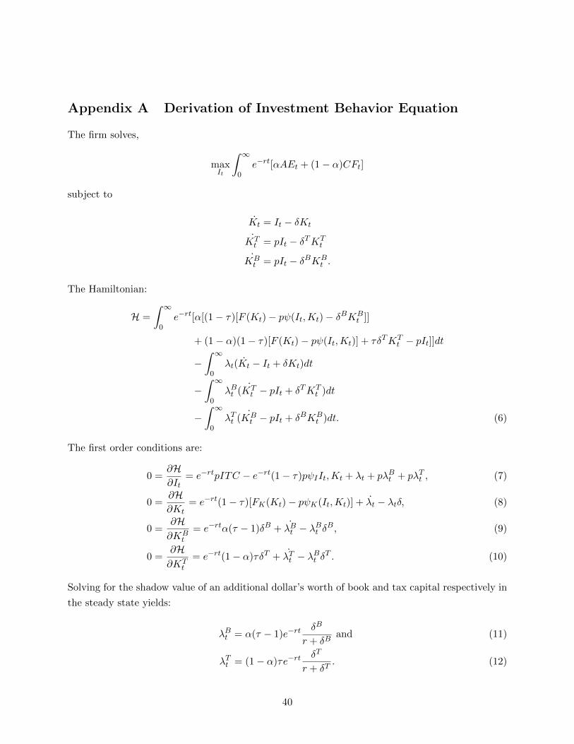
Appendix A Derivation of Investment Behavior Equation
The firm solves,
maxIt
∫ ∞0
e−rt[αAEt + (1− α)CFt]
subject to
K̇t = It − δKt
K̇Tt = pIt − δTKT
t
K̇Bt = pIt − δBKB
t .
The Hamiltonian:
H =
∫ ∞0
e−rt[α[(1− τ)[F (Kt)− pψ(It,Kt)− δBKBt ]]
+ (1− α)(1− τ)[F (Kt)− pψ(It,Kt)] + τδTKTt − pIt]]dt
−∫ ∞0
λt(K̇t − It + δKt)dt
−∫ ∞0
λBt (K̇Tt − pIt + δTKT
t )dt
−∫ ∞0
λTt (K̇Bt − pIt + δBKB
t )dt. (6)
The first order conditions are:
0 =∂H∂It
= e−rtpITC − e−rt(1− τ)pψIIt,Kt + λt + pλBt + pλTt , (7)
0 =∂H∂Kt
= e−rt(1− τ)[FK(Kt)− pψK(It,Kt)] + λ̇t − λtδ, (8)
0 =∂H∂KB
t
= e−rtα(τ − 1)δB + λ̇Bt − λBt δB, (9)
0 =∂H∂KT
t
= e−rt(1− α)τδT + λ̇Tt − λBt δT . (10)
Solving for the shadow value of an additional dollar’s worth of book and tax capital respectively in
the steady state yields:
λBt = α(τ − 1)e−rtδB
r + δBand (11)
λTt = (1− α)τe−rtδT
r + δT. (12)
40

For ease of notation, I define zB and zT as the present values of future depreciation allowances for
book and tax purposes, respectively,
zB =
∫ ∞0
e−rsδBe−δBs δB
r + δB
zT =
∫ ∞0
e−rsδT e−δT s δT
r + δT.
Plugging (8) and (9) into (4) and solving for the derivative of the adjustment cost function, λI ,
yields the investment behavior equation,
ψI =
λ0p0− ((1− α) + αzB − τ [(1− α)zT + αzB]− ITC
1− τ.
Appendix B Investment Control Variables
The marginal value of an additional dollar of investment (marginal Q), is measured as the ratio of
the market value of equity plus the book value of liabilities excluding deferred taxes, divided by
the book value of assets,
Qt =prcct × cshot + att − ceqt + txdbt
att,
Where prcc is the price of outstanding shares, csho is the number of outstanding shares, at is total
assets, ceq is outstanding equity and txdbt is the differed tax liabilities.
Measures of cash flow and financial distress are constructed following Kaplan and Zingales
(1997). ”Cash Flow/PPE” is defined as
Cash Flowt =ib18t + dp14t
ppent8t−1.
This ratio is the income before extraordinary items plus depreciation and amortization, scaled by
the capital stock at the beginning of the year.
The HP Index (Hadlock and Pierce (2010)) measures financial constraint as
HP Index = −0.737 ∗ size + 0.043 ∗ size2 − 0.04 ∗ age
where size = min{assets in 2004 dollars, $4.5 billion} and
age = min{years on Compustat tapes, 37}.
41

Appendix C Bonus Depreciation Legislation
• The Job Creation and Workers Assistance Act of 2002 enacted 30% bonus depreciation for
property placed into service after September 10, 2001.
• The Jobs and Growth Tax Relief Reconciliation Act of 2003 increased the bonus level to 50%
for property placed into service after May 5, 2003, and before January 1, 2005.
• Bonus depreciation expired December 31, 2004.
• The Economic Stimulus Act of 2008 reintroduced the bonus depreciation at a 50% rate for
capital placed into service after January 1, 2008.
• American Recovery and Reinvestment Act of 2009 extended the bonus at the 50% rate through
2009.
• The Small Business Jobs and Credit Act of 2010 further extended the depreciation at the
same rate through 2010. However, SBJCA was not signed into law until September 27, 2010,
so for the majority of 2010 businesses may have been under the impression that the bonus
depreciation might not be available on new capital expenditure.
• The Tax Relief and Unemployment Insurance Reauthorization and Job Creation Act of 2010
(signed on December 17, 2010) raised the bonus rate to 100% for property placed into service
after September 8, 2010, and before January 1, 2012. Property placed into service during
2012 garnered the 50% bonus.
• The American Taxpayer Relief Act of 2012 extended bonus depreciation at a rate of 50% for
2013.
42
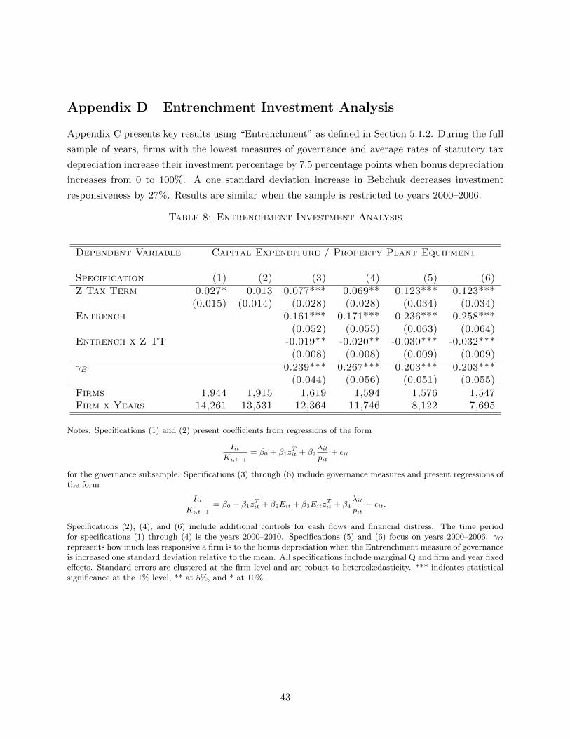
Appendix D Entrenchment Investment Analysis
Appendix C presents key results using “Entrenchment” as defined in Section 5.1.2. During the full
sample of years, firms with the lowest measures of governance and average rates of statutory tax
depreciation increase their investment percentage by 7.5 percentage points when bonus depreciation
increases from 0 to 100%. A one standard deviation increase in Bebchuk decreases investment
responsiveness by 27%. Results are similar when the sample is restricted to years 2000–2006.
Table 8: Entrenchment Investment Analysis
Dependent Variable Capital Expenditure / Property Plant Equipment
Specification (1) (2) (3) (4) (5) (6)
Z Tax Term 0.027* 0.013 0.077*** 0.069** 0.123*** 0.123***(0.015) (0.014) (0.028) (0.028) (0.034) (0.034)
Entrench 0.161*** 0.171*** 0.236*** 0.258***(0.052) (0.055) (0.063) (0.064)
Entrench x Z TT -0.019** -0.020** -0.030*** -0.032***(0.008) (0.008) (0.009) (0.009)
γB 0.239*** 0.267*** 0.203*** 0.203***(0.044) (0.056) (0.051) (0.055)
Firms 1,944 1,915 1,619 1,594 1,576 1,547Firm x Years 14,261 13,531 12,364 11,746 8,122 7,695
Notes: Specifications (1) and (2) present coefficients from regressions of the form
IitKi,t−1
= β0 + β1zTit + β2
λitpit
+ εit
for the governance subsample. Specifications (3) through (6) include governance measures and present regressions ofthe form
IitKi,t−1
= β0 + β1zTit + β2Eit + β3Eitz
Tit + β4
λitpit
+ εit.
Specifications (2), (4), and (6) include additional controls for cash flows and financial distress. The time periodfor specifications (1) through (4) is the years 2000–2010. Specifications (5) and (6) focus on years 2000–2006. γGrepresents how much less responsive a firm is to the bonus depreciation when the Entrenchment measure of governanceis increased one standard deviation relative to the mean. All specifications include marginal Q and firm and year fixedeffects. Standard errors are clustered at the firm level and are robust to heteroskedasticity. *** indicates statisticalsignificance at the 1% level, ** at 5%, and * at 10%.
43
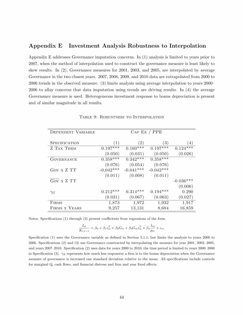
Appendix E Investment Analysis Robustness to Interpolation
Appendix E addresses Governance imputation concerns. In (1) analysis is limited to years prior to
2007, when the method of interpolation used to construct the governance measure is least likely to
skew results. In (2), Governance measures for 2001, 2003, and 2005, are interpolated by average
Governance in the two closest years. 2007, 2008, 2009, and 2010 data are extrapolated from 2000 to
2006 trends in the observed measure. (3) limits analysis using average interpolation to years 2000–
2006 to allay concerns that data imputation using trends are driving results. In (4) the average
Governance measure is used. Heterogeneous investment response to bonus depreciation is present
and of similar magnitude in all results.
Table 9: Robustness to Interpolation
Dependent Variable Cap Ex / PPE
Specification (1) (2) (3) (4)
Z Tax Term 0.197*** 0.160*** 0.197*** 0.124***(0.050) (0.031) (0.050) (0.026)
Governance 0.358*** 0.342*** 0.358***(0.076) (0.054) (0.076)
Gov x Z TT -0.042*** -0.041*** -0.042***(0.011) (0.008) (0.011)
Gov x Z TT -0.036***(0.006)
γG 0.212*** 0.314*** 0.194*** 0.290(0.031) (0.067) (0.063) (0.027)
Firms 1,873 1,972 1,932 1,917Firms x Years 9,257 13,131 8,684 16,859
Notes: Specifications (1) through (3) present coefficients from regressions of the form
IitKi,t−1
= β0 + β1zTit + β2Git + β3Gitz
Tit + β4
λitpit
+ εit.
Specification (1) uses the Governance variable as defined in Section 5.1.1, but limits the analysis to years 2000 to
2006. Specifications (2) and (3) use Governance constructed by interpolating the measure for year 2001, 2003, 2005,
and years 2007–2010. Specification (2) uses data for years 2000 to 2010; the time period is limited to years 2000–2006
in Specification (3). γB represents how much less responsive a firm is to the bonus depreciation when the Governance
measure of governance is increased one standard deviation relative to the mean. All specifications include controls
for marginal Q, cash flows, and financial distress and firm and year fixed effects.
44

Appendix F Governance and Shares Analysis
Appendix F presents specifications with both Governance and Shares variables and their interac-
tions with the Z Tax Term. Specifications (2) through (6) progressively limit analysis to firms that
are more likely to have professional managers.
Table 10: Baseline Analysis 2000–2010, Managerial Equity Percentage
Dependent Variable Capital Expenditure / Property Plant Equipment
Specification (1) (2) (3) (4) (5) (6)Shares Restriction < 20% < 15% < 10% < 5%
Z Tax Term 0.155*** 0.150*** 0.159*** 0.152*** 0.166*** 0.153***(0.031) (0.031) (0.032) (0.032) (0.034) (0.036)
Governance 0.315*** 0.321*** 0.324*** 0.323*** 0.334*** 0.310***(0.054) (0.056) (0.057) (0.058) (0.060) (0.064)
Gov x Z TT -0.039*** -0.040*** -0.040*** -0.040*** -0.042*** -0.040***(0.008) (0.008) (0.008) (0.008) (0.008) (0.009)
Shares -0.000 -0.003 0.023 0.008 0.041* 0.070(0.006) (0.006) (0.016) (0.018) (0.024) (0.044)
Shares x Z TT 0.000 0.000 -0.003 -0.001 -0.006 -0.010(0.001) (0.001) (0.002) (0.003) (0.004) (0.007)
Firms 1,619 1,592 1,571 1,557 1,526 1,453Firms x Years 12,364 11,926 11,535 11,348 10,992 10,071
Notes: Table 5 presents regressions of the form
IitKi,t−1
= β0 + β1τzTit + β2Git + β3Gitτz
Tit + β3Sit + β4Sitτz
Tit + β5
λitpit
+ εit.
Specifications (2) through (6) include additional controls for financial distress and cash flows. All specifications include
firm and year fixed effects. Standard errors are clustered at the firm level and are robust to heteroskedasticity. ***
indicates statistical significance at the 1% level, ** at 5%, and * at 10%.
45

Appendix G Decomposing the Governance Index
In Appendix G, the effect of Governance Sub-Indexes are analyzed separately.
Table 11: Decomposing the Governance Index
Dependent Variable Capital Expenditure / Property Plant Equipment
Specification (1) (2) (3) (4) (5) (6)
Z Tax Term 0.050 -0.013 0.117*** 0.118*** 0.221*** 0.379***(0.043) (0.018) (0.023) (0.029) (0.042) (0.061)
Voting 0.062 0.092(0.059) (0.059)
Voting x ZTT -0.009 -0.013(0.008) (0.008)
Delay -0.108* -0.213***(0.057) (0.066)
Delay x ZTT 0.016** 0.030***(0.008) (0.009)
Protection 0.400*** 0.319***(0.059) (0.059)
Protection x ZTT -0.052*** -0.041***(0.008) (0.008)
State 0.148*** 0.118***(0.034) (0.034)
State x ZTT -0.022*** -0.018***(0.005) (0.005)
Other 0.524*** 0.454***(0.088) (0.103)
Other x ZTT -0.065*** -0.056***(0.012) (0.014)
Notes: Specifications (1) through (5) present coefficients from regressions of the form:
IitKi,t−1
= β0 + β1zTit + β2Git + β3Gituz
Tit + β4
λitpit
+ εit.
Specification (6) includes all sub-indexes and their interaction with the Z Tax Term. All specifications include marginal
Q and firm and year fixed effects. Standard errors are clustered at the firm level and are robust to heteroskedasticity.
*** indicates statistical significance at the 1% level, ** at 5%, and * at 10%. i = 1, 911, i× t = 13, 704.
46
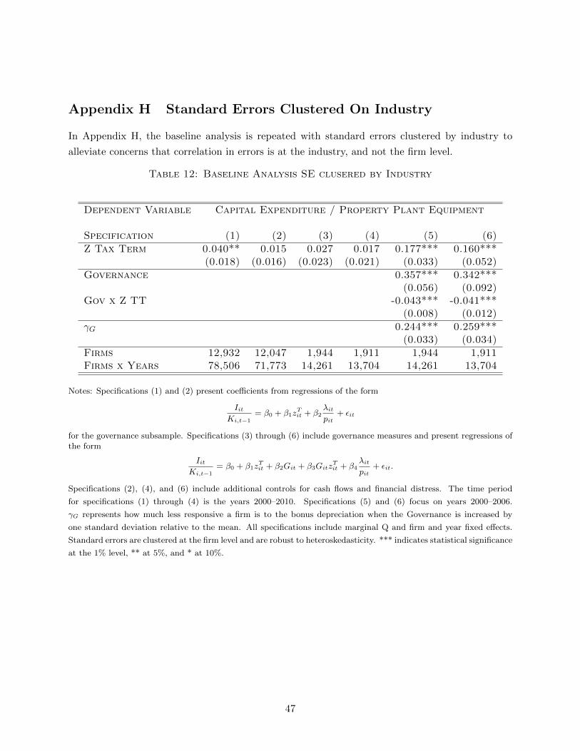
Appendix H Standard Errors Clustered On Industry
In Appendix H, the baseline analysis is repeated with standard errors clustered by industry to
alleviate concerns that correlation in errors is at the industry, and not the firm level.
Table 12: Baseline Analysis SE clusered by Industry
Dependent Variable Capital Expenditure / Property Plant Equipment
Specification (1) (2) (3) (4) (5) (6)
Z Tax Term 0.040** 0.015 0.027 0.017 0.177*** 0.160***(0.018) (0.016) (0.023) (0.021) (0.033) (0.052)
Governance 0.357*** 0.342***(0.056) (0.092)
Gov x Z TT -0.043*** -0.041***(0.008) (0.012)
γG 0.244*** 0.259***(0.033) (0.034)
Firms 12,932 12,047 1,944 1,911 1,944 1,911Firms x Years 78,506 71,773 14,261 13,704 14,261 13,704
Notes: Specifications (1) and (2) present coefficients from regressions of the form
IitKi,t−1
= β0 + β1zTit + β2
λitpit
+ εit
for the governance subsample. Specifications (3) through (6) include governance measures and present regressions ofthe form
IitKi,t−1
= β0 + β1zTit + β2Git + β3Gitz
Tit + β4
λitpit
+ εit.
Specifications (2), (4), and (6) include additional controls for cash flows and financial distress. The time period
for specifications (1) through (4) is the years 2000–2010. Specifications (5) and (6) focus on years 2000–2006.
γG represents how much less responsive a firm is to the bonus depreciation when the Governance is increased by
one standard deviation relative to the mean. All specifications include marginal Q and firm and year fixed effects.
Standard errors are clustered at the firm level and are robust to heteroskedasticity. *** indicates statistical significance
at the 1% level, ** at 5%, and * at 10%.
47
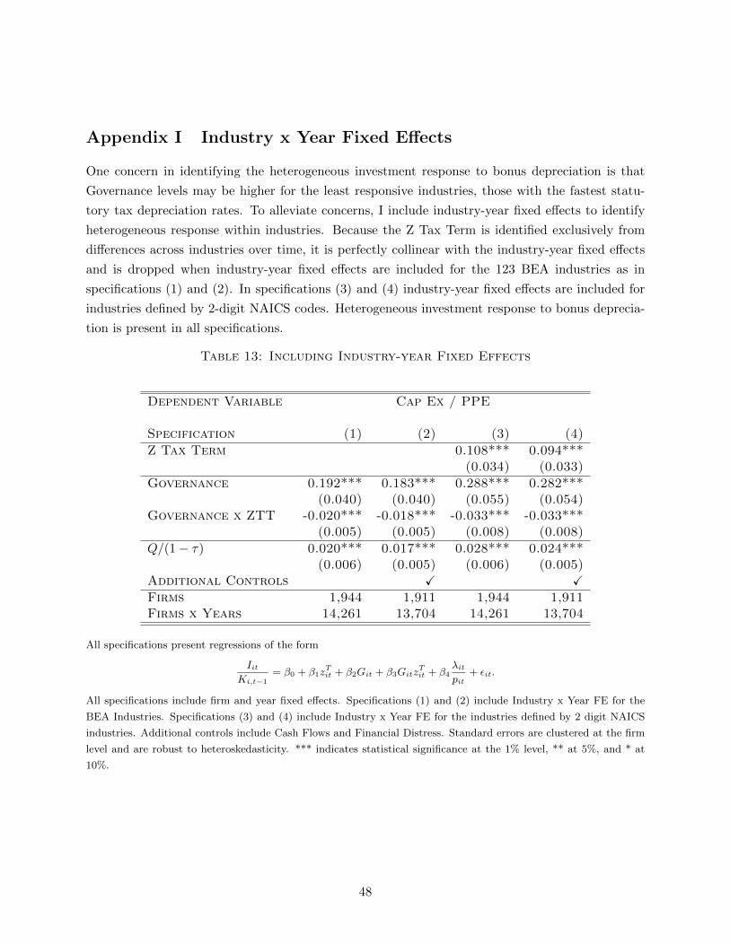
Appendix I Industry x Year Fixed Effects
One concern in identifying the heterogeneous investment response to bonus depreciation is that
Governance levels may be higher for the least responsive industries, those with the fastest statu-
tory tax depreciation rates. To alleviate concerns, I include industry-year fixed effects to identify
heterogeneous response within industries. Because the Z Tax Term is identified exclusively from
differences across industries over time, it is perfectly collinear with the industry-year fixed effects
and is dropped when industry-year fixed effects are included for the 123 BEA industries as in
specifications (1) and (2). In specifications (3) and (4) industry-year fixed effects are included for
industries defined by 2-digit NAICS codes. Heterogeneous investment response to bonus deprecia-
tion is present in all specifications.
Table 13: Including Industry-year Fixed Effects
Dependent Variable Cap Ex / PPE
Specification (1) (2) (3) (4)
Z Tax Term 0.108*** 0.094***(0.034) (0.033)
Governance 0.192*** 0.183*** 0.288*** 0.282***(0.040) (0.040) (0.055) (0.054)
Governance x ZTT -0.020*** -0.018*** -0.033*** -0.033***(0.005) (0.005) (0.008) (0.008)
Q/(1− τ) 0.020*** 0.017*** 0.028*** 0.024***(0.006) (0.005) (0.006) (0.005)
Additional Controls X XFirms 1,944 1,911 1,944 1,911Firms x Years 14,261 13,704 14,261 13,704
All specifications present regressions of the form
IitKi,t−1
= β0 + β1zTit + β2Git + β3Gitz
Tit + β4
λitpit
+ εit.
All specifications include firm and year fixed effects. Specifications (1) and (2) include Industry x Year FE for the
BEA Industries. Specifications (3) and (4) include Industry x Year FE for the industries defined by 2 digit NAICS
industries. Additional controls include Cash Flows and Financial Distress. Standard errors are clustered at the firm
level and are robust to heteroskedasticity. *** indicates statistical significance at the 1% level, ** at 5%, and * at
10%.
48
Appendix J Taxable Status and Investment Response
Firms that have tax loss carry-forwards should be unresponsive to bonus depreciation. If firms are
strongly governed because they have performed poorly in the past, then the most strongly governed
firms are likely to have tax loss-carry-forwards and should be unresponsive to bonus depreciation.
In this case, empirical analysis excluding measures of tax status would show that strongly governed
firms are less responsive to bonus depreciation. To alleviate concerns of this nature, I include
three different measures of tax status and tax status interacted with the Z Tax Term to baseline
regressions.
1(TLCF) The first measure of taxable status is an indicator for whether the firm has any tax
loss carry-forwards. The variable is equal to 1 when the firm reports a positive number of tax loss
carry-forwards. The indicator is equal to zero if the firm reports 0 tax loss carry forwards or if the
value is missing but the firm reports a positive number for Property Plant and Equipment. When
the indicator is turned on, firms should be less responsive to bonus depreciation.
TLCF The second measure of taxable status is the level of tax loss carry-forwards reported by the
firm. The variable is set equal to zero if the value is missing but the firm reports a positive number
for Property Plans and Equipment. When firms have more tax loss carry-forwards, they should be
less responsive to bonus depreciation. I scale this variable to be a number between 0 and 100.
MTR The third measure of taxable status is a simulated marginal tax rate constructed by Blouin,
Core and Guay (2010). I use the marginal tax rate after interest deductions have been accounted
for. When this number is higher, firms should be more responsive to bonus depreciation. The
simulated tax rates take on values between 0 and 1.
I perform analysis using both contemporaneous taxable status measure and once-lagged mea-
sures to control for potential endogenous. Odd-numbered specifications reported below use the
contemporaneous tax status measure. Even-numbered specifications use the lagged tax status.
The results of the tax-status analysis continue to show substantial heterogeneity in investment
response to bonus depreciation. The magnitude of the heterogeneity is similar to the magnitude of
the heterogeneity in the baseline results. The regression analysis also indicates that taxable status
plays a role in determining investment response to bonus depreciation. Specification (1) results
suggest that firms that have tax loss carry-forwards are more than 50% less responsive to bonus
depreciation. Specification (5) results suggest that a 10% increase in simulated marginal tax rates
makes firms approximately 50% more responsive to bonus depreciation.
49
Appendix K Reconciling Investment and Event Study Results
This appendix uses investment response results to predict stock market price responses to the 50%
bonus deprecation extension analyzed in Section 7.
• Using results from the investment response analysis, the effect extension of bonus depreciation
at a rate of 50% can be calculated. According the the investment response results, for a firm
with the average level of governance, investment does not respond to bonus depreciation. For
the average firm, the benefit of bonus depreciaiton comes exclusively from decreases in the net
present value costs of investment. For a firm with mean Deprec, 50% bonus decreases NPV
investment price by $0.21. For the average firm in the sample, this amounts to a decrease of
$6.573 million and results in a net income of 2.08%. For a firm that invests in longer-lived
equipment and has Deprec one standard deviation below the mean, the cost of investment
decreases by $0.035 per dollar which decreases the cost of investment by $10.995 million and
increases income by 3.47%. Under the overly-simple assumption that income is a perfect
proxy for firm value, upon announcement of 50% bonus depreciation, the value of firms that
have one standard deviation lower Deprec should increase by 1.39% more than firms with
mean Deprec levels. This is the exact interpretation of the Deprec coefficient in the event
study analysis. The event study analysis found this number to be 0.644%.
• As the level of governance decreases, bonus depreciation is more effective at stimulating
investment. While the firm with mean levels of governance does not increase investment
in response to bonus deprecation, a firm with governance one standard deviation below the
mean increases investment percent by 2.85% in response to 50% bonus depreciation. This
increase is equivalent to $8.921 million in additional investment. Using marginal Q to translate
investment into firm value, this investment response increases the value of the less-governed
firm by $25.38 million or 0.46% of the value of the average firm in the sample. The event
study analysis concludes firm values with governance levels one standard deviation below the
mean experience abnormal returns of 0.457 % more than firms with mean governance levels.
50
Appendix L Investment Impact of ITC Repeal
In this section, I test a secondary hypothesis of the theoretical model presented in Section 4. The
model predicts that while investment response should be heterogeneous to bonus depreciation via
the Z Tax Term, investment should not be heterogeneous in response to investment tax credits,
which affect both flows and accounting earnings;
∂I/K
∂ITC=
1
1− τ∂I/K
∂τzT=
1− α1− τ
.
If, in fact, investment response to ITC is not heterogeneous across firms with varying levels of
governance, then there is additional evidence that bonus depreciation take-up is limited due to its
accounting interactions and that bonus depreciation is a nice natural experiment to test for the
relationship between governance and earnings management.
To test the theory, I will run regressions of the form
IitKi,t−1
= β0 + β1ITCTit1− τt
+ β2τzTit
1− τt+ β3
GitITCTit
1− τt+ β4
GitτzTit
1− τt+ β5
λitpit− 1
1− τt
on data that includes changing tax depreciation rates and investment tax credits. If the coefficient
β3 is equal to zero, then the subsidiary model prediction is confirmed. Coefficient β4 should be
greater than zero if investment response to changes in statutory depreciation rates is heterogeneous
in the governance measure. However, I expect to find no heterogeneous response, because statutory
tax depreciation rates were not the primary investment stimulus tool used during the new sample
period; the ITC was.
The ITC was retroactively repealed in 1985 by The Tax Reform Act of 1986. This analysis will
focus on the period around the repeal, years 1981 to 1987, three years prior to and three years after
repeal. During this time, top statutory tax rates and statutory depreciation rates were also in flux.
The analysis accounts for these changes.
Governance Data: The IRRC began collecting corporate governance data in 1990. This data will
be projected back to the time sample of interest. This presents possible measurement error into the
analysis. However, as Gompers et al. (2003) pointed out, governance variables are relatively stable
over time. I will test both the Governance and Entrenchment measures in the following analysis.
Tax Variables: I construct the Z Tax Term as in Section 4. The construction of the investment
tax credit variable,
ITC Tax Term =ITCit
1− τt,
51
is similar. Dale Jorgenson provides ITC data on 44 different types of assets. For each asset class,
both the ITC rate, which varies over time, and the ITC basis (whether the type of asset qualified for
the tax credit) is provided. Using the 1982 BEA Capital Flow Table, the percentage of investment
in each asset type by each industry is constructed. These weights are combined with ITC rates
and bases to create industry-level ITC rates that vary over time. Variation over time in the ITC
is driven by reforms in 1982 and 1985, when the ITC was ultimately (and retroactively) repealed.
Variation across industries is driven by the percentage of investment eligible for the tax credit in
each industry. The impact of the investment tax credit is identified by industry-level differences
in the percentage of capital expenditures that are eligible for the investment tax credit. When
the credit is repealed in 1985, it is most detrimental to the industries where a large percentage of
capital expenditure used to be eligible for the credit.
Other Data: All other variables are constructed as in Section 5.
Table L1 provides descriptive statistics for the 1981-1987 analysis. The Governance sample are
larger firms for which the governance variables are available. These firms tend to invest less as a
percentage of capital. They also have larger cash flows. The investment tax credit ranges from 0
to 10% over the sample, 0 to 0.187 when scaled by the top statutory tax rate.
Results: Table L2 provides regression results for the 1981–1987 ITC analysis. Specifications (1)
and (2) examine the effect of the ITC Tax Term and the Z Tax Term for the full sample with
and without additional controls. The results suggest that the general population of firms is very
responsive to changes in both investment tax credits and depreciation allowances. When the sample
is limited to the Governance Sample in specifications (3) and (4), the results are less extreme and
not statistically different from zero. This is most likely due to the small sample size.
In specification (5), Governance, Governance interacted with the ITC Tax Term, and Gov-
ernance interacted with the Z Tax Term are added to the regression. The coefficients on the
interaction terms are not statistically different from zero for either tax variable, suggesting no
heterogeneity in response to changes in either type of investment tax incentives. Specification
(6) repeats the analysis using the Entrenchment governance variable. Results are similar, again
suggesting no heterogeneity of response.
While this analysis is plagued by a relatively small sample size and possible mismeasurement of
the governance variables, it does not strongly contradict the main results presented in this paper.
If this analysis found that strongly governed firms decreased their investment behavior the least
when the investment tax credit was repealed, it would call into question the heterogeneity that
supports the connection between governance and earnings management.
52

Table 14: Investment Responsiveness and Tax Status
Dependent Var Capital Expenditure / Property Plant Equipment
Specification (1) (2) (3) (4) (5) (6)
Z Tax Term 0.165*** 0.161*** 0.182*** 0.156*** 0.055 0.054(0.032) (0.032) (0.042) (0.040) (0.056) (0.057)
Gov x Z TT -0.041*** -0.040*** -0.043*** -0.040*** -0.038*** -0.039***(0.008) (0.007) (0.010) (0.009) (0.007) (0.008)
1(TLCF) 0.168* 0.143(0.098) (0.104)
1(TLCF) x Z TT -0.025* -0.022(0.014) (0.015)
TLCF 0.006 -0.002(0.004) -0.002
TLCF x Z TT -0.001* -0.000(0.001) (0.001)
MTR -1.390 -1.285(1.004) (0.968)
MTR x ZTT 0.263* 0.256*(0.145) (0.140)
Firms 1,911 1,911 1,471 1,479 1,809 1,810Firms x Years 13,704 13,692 8,505 8,534 13,080 13,113
Notes: All specifications present coefficients from regressions of the form
IitKi,t−1
= β0 + β1zTit + β2Git + β3Gitz
Tit + β4TAXit + β5TAXτzTit + β6
λitpit
+ εit.
Where TAX is an indicator for tax loss carry-forwards in specifications (1) and (2), is the level of tax loss carry-
forwards in (3) and (4), and is the Blouin et al. (2010) estimated marginal tax rate in (5) and (6). Specifications
(2), (4), and (6) use the lagged tax variable to avoid endogeneity concerns. All specifications control for marginal Q,
financial distress, and cash flows and include firm and year fixed effects. Standard errors are clustered at the industry
level and are robust to heteroskedasticity. *** indicates statistical significance at the 1% level, ** at 5%, and * at
10%.
53
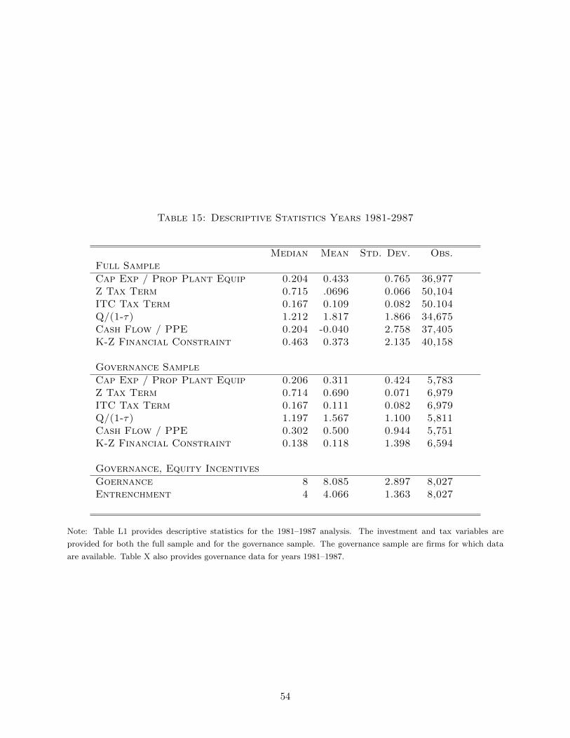
Table 15: Descriptive Statistics Years 1981-2987
Median Mean Std. Dev. Obs.Full Sample
Cap Exp / Prop Plant Equip 0.204 0.433 0.765 36,977Z Tax Term 0.715 .0696 0.066 50,104ITC Tax Term 0.167 0.109 0.082 50.104Q/(1-τ) 1.212 1.817 1.866 34,675Cash Flow / PPE 0.204 -0.040 2.758 37,405K-Z Financial Constraint 0.463 0.373 2.135 40,158
Governance Sample
Cap Exp / Prop Plant Equip 0.206 0.311 0.424 5,783Z Tax Term 0.714 0.690 0.071 6,979ITC Tax Term 0.167 0.111 0.082 6,979Q/(1-τ) 1.197 1.567 1.100 5,811Cash Flow / PPE 0.302 0.500 0.944 5,751K-Z Financial Constraint 0.138 0.118 1.398 6,594
Governance, Equity Incentives
Goernance 8 8.085 2.897 8,027Entrenchment 4 4.066 1.363 8,027
Note: Table L1 provides descriptive statistics for the 1981–1987 analysis. The investment and tax variables are
provided for both the full sample and for the governance sample. The governance sample are firms for which data
are available. Table X also provides governance data for years 1981–1987.
54

Table 16: Investment Tax Credit Analysis 1981–1987
Dependent Variable Capital Expenditure / Property Plant Equipment
Specification (1) (2) (3) (4) (5) (6)
ITC Tax Term 3.794*** 3.730*** 1.143 0.770 0.336 0.297(1.347) (1.238) (1.386) (1.367) (1.369) (1.352)
Z Tax Term 4.060*** 3.407*** 1.620* 0.943 1.029 0.963(0.981) (0.941) (0.942) (0.908) (1.410) (1.361)
Gov x ITC TT 0.049(0.069)
Gov x Z TT 0.002(0.181)
Entrench x ITC TT 0.097(0.114)
Entrench x Z TT 0.009(0.308)
Q/(1− τ) 0.024*** 0.026*** 0.077*** 0.039* 0.039** 0.038*(0.006) (0.007) (0.023) (0.020) (0.020) (0.020)
Additional Controls X X X XFirms 7,497 7,280 988 950 950 950Observations 30,126 29,299 5,340 5,222 5,222 5,222
Notes: Specifications (1) through (4) present regressions of the form
IitKi,t−1
= β0 + β1ITCTit1 − τt
+ β2τzTit
1 − τt+ β3
λitpit
1 − τt.
Specifications (5) and (6) include governance measures and present regressions of the form
IitKi,t−1
= β0 + β1ITCTit1 − τt
+ β2τzTit
1 − τt+ β3
GitITCTit
1 − τt+ β4
GitτzTit
1 − τt+ β5
λitpit
− 1
1 − τt.
All specifications include the structures tax term. Specifications (2) and (4) through (6) include additional controlsfor cash flow and financial distress.
All specifications include firm and year fixed effects. Standard errors are clustered at the firm level and are robust to
heteroskedasticity. *** indicates statistical significance at the 1% level, ** at 5%, and * at 10%.
55

Appendix M Event Study Placebo Tests
Table 17: Event Study Placebos
Event Study Placebo 1: December 10, 2012
Dependent Variable CAR1 CAR2 CAR3 CAR4 CAR5 CAR6
Bebchuk 0.049 -0.001 0.042 0.046 0.085 0.128(0.042) (0.058) (0.073) (0.079) (0.072) (0.084)
Deprec -0.030 0.217* 0.345* 0.382 0.203 0.168(0.108) (0.129) (0.206) (0.260) (0.180) (0.194)
Bebchuk x Deprec -0.063 0.012 0.152 0.121 0.149 -0.063(0.088) (0.117) (0.137) (0.146) (0.126) (0.137)
Observations 1,189 1,189 1,189 1,189 1,189 1,189
Event Study Placebo 2: January 15, 2013
Dependent Variable CAR1 CAR2 CAR3 CAR4 CAR5 CAR6
Bebchuk 0.017 0.095 0.055 0.037 0.030 0.024(0.048) (0.066) (0.097) (0.111) (0.135) (0.157)
Deprec -0.143 -0.157 -0.238 -0.331 -0.339 -0.214(0.213) (0.424) (0.411) (0.528) (0.516) (0.577)
Bebchuk x Deprec -0.054 -0.012 0.145 0.244 0.305 0.214(0.065) (0.097) (0.110) (0.152) (0.193) (0.204)
Observations 1,189 1,189 1,189 1,189 1,189 1,189
Nottes: CARt is the cumulative abnormal return t trading days after Pacebo Dates December 10, 2012 and January
15, 2013. Results include industry fixed effects and control for Cash Flow. Standard errors are clustered at the firm
level and are robust to heteroskedasticity. *** statistical significance 1% level, ** at 5%, and * at 10%.
56