Un i ve r s i t y o f Kons t an z Depa r tmen t o f E c onom i c s

http://www.wiwi.uni-konstanz.de/workingpaperseries

Working Paper Series 2010-16

Does Government Ideology Influence Budget Composition? Empirical Evidence from OECD Countries

Niklas Potrafke

Does government ideology influence budget composition?

Empirical evidence from OECD countries

Niklas Potrafke1 University of Konstanz

This version: December 13, 2010

Abstract

This paper examines whether government ideology has influenced the allocation of public

expenditures in OECD countries. I analyze two datasets that report different expenditure

categories and cover the time periods 1970-1997 and 1990-2006, respectively. The results

suggest that government ideology has had a rather weak influence on the composition of

governments’ budgets. Leftist governments, however, increased spending on “Public

Services” in the period 1970-1997 and on “Education” in the period 1990-2006. These

findings imply, first, that government ideology hardly influenced budgetary affairs in the last

decades, and thus, if ideology plays a role at all, it influences non-budgetary affairs. Second,

education has become an important expenditure category for leftist parties to signal their

political visions to voters belonging to all societal groups.

Keywords: budget composition, public expenditures, government ideology, partisan politics,

education policy, panel data

JEL Classification: D72, H50, H61, I28, C23

1 University of Konstanz, Department of Economics, Box 138, D-78457 Konstanz, Germany, Phone: + 49 7531 88 2137, Fax: + 49 7531 88 3130. Email: niklas.potrafke@uni-konstanz.de

2

1. Introduction

Investigating the determinants of public spending is one of the prominent topics of

Public Economics. While previous research has focused on the size of government, many

scholars have recently also investigated the composition of public expenditures. Political

institutions have been shown to be important determinants of budget composition. Lago-

Peñas and Lago-Peñas (2009), for example, show that party linkage or the nationalization of

party systems (as measured by the effective number of parties at the national level in relation

to the effective number at the district level) has influenced budget composition in 18 Western

European countries in the period 1970-1998. The reason is that in weakly nationalized party

systems, sub national parties are important veto players that impede changes in the national

budget composition. In Argentina, presidents have distributed capital expenditures (the more

flexible item of the National Budget) to their home provinces and provinces administered by

governors affiliated with their party (Bercoff and Meloni 2009). By contrast, globalization has

hardly influenced budget composition (Dreher et al. 2008a, 2008b, Sanz and Velázquez 2007,

Gemmell et al. 2008, Shelton 2007). The influence of government ideology on the

composition of public spending, on the other hand, has been completely ignored in cross

national studies. Scholars have investigated how government ideology has influenced the

composition of public expenditures at the state level in federal states such as Canada (e.g.,

Kneebone and McKenzie 2001) or Germany (e.g., Potrafke 2011a). Given the importance of

ideology-induced preferences in designing government budgets, this is a surprising omission.

Another reason for manipulating the budget are electoral considerations. In this paper,

however, I will focus on the influence of government ideology and do not investigate electoral

cycles (see, e.g., Vergne 2009 , Katsimi and Sarantides 2010).

Budgets are often considered to represent government programs in numbers. The

revenues and the need to service predetermined budget positions notwithstanding, each

government can choose its spending priorities. Governments are not able to change budgets

3

completely, of course. Path dependence and long-run spending commitments influence public

expenditures (see, for example, Rose´s 1990 “inheritance before choice” in public policy).

The composition of the budget will however reflect the preferences of the government and its

constituencies. Leftwing and rightwing governments are expected to place emphasis on

different budget positions with a view to gratifying their clientele.2

Many scholars have investigated how government ideology influences the size of

government as measured by the government budget in OECD panels, but they have not

examined the composition of the budget. To be sure, I acknowledge that Bräuninger (2005)

introduces a partisan model of government expenditures and provides empirical evidence for

the period 1971-1999, distinguishing only two expenditure categories. His results suggest that

the actual spending preferences of parties matter, but these preferences do not appear to be

governed by a clear-cut left-right alignment. Evaluating whether leftwing and rightwing

governments set other budget priorities requires analyzing many expenditure categories that

mirror various policy fields. The more comprehensive the classifications of government

expenditure, the higher the probability that policy effects remain undetected.

In this paper, I employ the COFOG (Classification of the Functions of Government)

classifications of government functions. I analyze the dataset by Sanz and Velázquez (2007)

that covers the period 1970-1997, and a more recent OECD dataset covering the period 1990-

2006 in order to examine whether government ideology had an influence on the allocation of

public expenditures. The results suggest that government ideology has had a rather weak

influence on the composition of government budgets. Leftist governments, however,

increased spending on “Public Services” in the period 1970-1997 and on “Education” in the

period 1990-2006. These findings imply, first, that government ideology hardly influenced

budgetary affairs in the last decades, and thus, if ideology plays a role at all, it influences non-

2 On the influence of party alternation of fiscal performance see, for example, Calcagno and Escaleras (2007).

4

budgetary affairs. Second, education has become an important expenditure category for leftist

parties to signal their political visions to voters belonging to all societal groups.

The paper is organized as follows: Section 2 discusses theoretical and empirical

studies on the partisan approach and budget composition. Section 3 presents the data. Section

4 specifies the empirical model. Section 5 reports and discusses the estimation results, and

investigates their robustness. Section 6 concludes.

2. Government ideology and budget composition

Politicians’ behavior is expected to affect economic policy. The political business

cycle and partisan theories indicate how politicians will influence economic outcomes.3 The

partisan approach focuses on the role of party ideology and shows to what extent leftwing and

rightwing politicians can pursue different policies that reflect the preferences of their partisan

constituencies. Leftist parties appeal more to the labor base and promote expansionary fiscal

and monetary policies, whereas rightwing parties appeal more to capital owners, and are

therefore more concerned with reducing inflation. This holds for both branches of the partisan

theory - for the classical approach (Hibbs 1977) and for the rational approach (Alesina 1987).

For empirical evaluations of the partisan theories see, e.g., Alesina et al. (1997), Sakamoto

(2008), Heckelman (2002), Tavares (2004), Bjørnskov (2008a), Potrafke (2011b).4

In addition to determining the size of the budget, parties also determine the allocation

of specific government spending with a view to gratifying their clientele (Bräuninger 2005,

Drazen and Eslava 2010). A key difference between leftwing and rightwing parties concerns

their different views on taxation, public good provision and income redistribution. Individuals

3 One implication of the political business cycle theories (Nordhaus 1975 and Rogoff and Sibert 1988, among

others) is that all politicians will implement the same expansionary economic policy before elections. For theoretical enhancements and empirical evaluations see, for example, Shi and Svensson (2006) or Angelopoulos and Economides (2008). 4 Yet there is no conclusive empirical evidence that leftist governments in fact promote more expansionary

policies. The results by Alt and Lassen (2006), for example, suggest that right-wing governments tend to have higher deficits than left-wing governments.

5

with a high income and high skills, which are associated with rightwing parties, are expected

to lobby for public expenditures spent on public good provision, just in order to prevent

public money from being spent on transfers. In a similar vein, individuals with a low income

and low skills, which are associated with leftwing parties, are expected to lobby against public

expenditures on public good provision, because it implies a reduction of direct income

transfers (Bierbrauer 2009).

Social policy has traditionally been politically controversial. Hicks and Swank (1992),

for example, provide theory and evidence to describe how policy influences welfare spending

in industrialized countries. Following the social democratic corporatist perspective, leftwing

and centrist government parties generate higher welfare efforts than rightwing and

“intermediate” parties. Scholars have extensively investigated how government ideology has

influenced social policy and many have focused on overall social expenditures. Empirical

evidence detects higher social expenditures under leftist than rightwing governments till the

end of the “cold war” in 1990, whereas partisan effects disappeared in the 1990s (e.g., Kittel

and Obinger 2003, Potrafke 2009a, Congleton and Bose 2010). The reason is that all parties

reduced social expenditures compared to the period 1960-1980s (e.g. Huber and Stephens

2001, Pierson 1996 and 2001). Over the period 1980-2005, leftwing governments somewhat

delayed social expenditure cutbacks in OECD countries (Tepe and Vanhuysse 2010). In

traditionally leftwing countries such as the Scandinavian countries, rightwing governments

have however been shown to spend more on social welfare than leftwing governments. This is

because rightwing governments are forced to compensate for the lack of public trust by being

even more generous than leftwing governments (Jensen 2010). All that notwithstanding, I

hypothesize that leftwing government favor higher total social spending.

In a similar vein, leftist governments are expected to increase the role of government

in health policy and therefore increase public health expenditures. Immergut (1992: 1)

describes how politicians implement different health policies and comes to the following

6

conclusion: “National health insurance symbolizes the great divide between liberalism and

socialism, between the free market and the planned economy…Political parties look to

national health insurance programs as a vivid expression of their distinctive ideological

profiles and as an effective means of getting votes National health insurance, in sum, is a

highly politicized issue.” De Donder and Hindricks (2007) examine the political economy of

social insurance policy and demonstrate that in a two party model, the leftwing party proposes

more social insurance than the rightwing party. The rightwing party attracts the richer

individuals, and those with smaller health risks, and the leftwing party attracts the poorer

individuals, and those with higher health risks.

By contrast, Jensen (2011a) argues that in modern welfare states, both leftwing and

rightwing parties expand public health spending. While previous studies have established

theories how leftwing governments extend the public health system and considered rightwing

governments only as counterparts to leftwing governments, Jensen (2011a) explicitly

develops a theory how rightwing governments implement health policies. Rightwing

governments face the following dilemma: they need to consider the pro-public preferences of

the important middle-class voters and the preferences of the pro-private preferences of the

high-income voters. Moreover, in almost all industrialized countries except the United States,

compulsory public health systems have been established. A majority of the voters appears to

be strictly against severe cuts in the public health system.5 Rightwing governments are

expected to solve this dilemma by a strategy called “marketization via compensation”. This

strategy consists of two components. First, rightwing governments match health policies of

the political left and keep public health spending at a quite high level. Second, rightwing

governments actively encourage and financially support private market health care such as

5 After overall public spending had increased in the course of the recession in the beginnings of the 1980s, the

rightwing governments lead by Margret Thatcher and Ronald Reagan eventually curbed social transfers and cut public spending on capital formation and industrial subsidies. Spending on social affairs, however, was not reduced. (Boix 1998: 192) explains this strategy as follows: “Strict electoral calculations partially explain the Conservatives’ conscious rejection of any substantial reduction in core welfare programs to achieve their overall goal of lower public expenditure. Popular support for the welfare state was just too strong.”

7

indirect support of private health insurance. The empirical results by Jensen (2011a, 2011b)

and Potrafke (2010a) show that government ideology has not influenced public health

expenditures in OECD countries. In a similar vein, the results by Tepe and Vanhuysse

(2009b: footnote 5) suggest that government ideology did not influence pension expenditures

in OECD countries.

Political ideology also influences environmental policy. Leftwing parties and, in

particular, leftist Green parties, have put emphasis on environmental protection. The model by

Cremer et al. (2008), for example, predicts that leftwing parties (Democrats) propose higher

emission tax rates than rightwing parties (Republicans) if intra-party polarization is high and

the militant party faction dominates the overall party profile. If the opportunistic (election-

motivated) party faction dominates the overall party profile, both the leftwing and the

rightwing party offer the same emission tax rate (Cremer et al. 2008 do not test this claim

empirically). Conventional wisdom is that leftwing parties are more active in environmental

protection. Christian Democratic parties are, however, concerned, about the integrity of the

divine creation and are thus also concerned about environmental quality.6 Policy platforms of

traditional parties (Social Democrats and Christian Democrats) and Green Parties have

converged in the last decades. Laurency and Schindler (2010) show that international climate

agreements that reduce greenhouse gas emissions and decrease effective abatement costs have

induced convergence in policy platforms: the higher is the flexibility and cost reduction in

international agreements, the more Green parties lose their unique green policy position

because non-Green parties will be more flexible in adjusting their party platforms.

The relationship between government ideology and public spending on economic

affairs appears to be ambiguous. Leftwing and rightwing governments have different

preferences on the size and scope of government and thus on economic policy. Leftwing

governments are in favor of strongly regulating the economy. In contrast, rightwing 6 Ono (2009) discusses intergenerational conflicts about the composition of public spending over environmental

investment and social security.

8

governments believe in the free market and thus favor less state intervention.7 For this reason,

spending on economic affairs should be lower under rightwing than under leftwing

governments. Spending on economic affairs includes, however, spending on fuel and energy

industries as well as agriculture. These industries appear to be more associated with rightwing

than leftwing parties.8

Leftist governments are expected to spend more on education than conservative

governments. The significant difference between leftwing and rightwing governments in the

education system is that leftwing governments favor the expansion of public authority in the

education system, whereas rightwing governments favor private alternatives (Busemeyer

2009a). In Switzerland, for example, social democratic ideology has had a negative influence

on privatizing education (Merzyn and Ursprung 2005). Scholars have recently investigated

the influence of government ideology on total education spending and mostly find that overall

education spending was higher under leftwing governments in OECD countries (Boix 1997,

Schmidt 2007, Busemeyer 2007 and 2009a, and Ansell 2008). By contrast, the results by

Jensen (2011c) do not suggest that overall education spending was higher under leftwing

governments in the period 1980-2000 in OECD countries. Jensen´s (2011c) argument

confronts with the so called “Boix model” predicting that total education spending is higher

under social democratic governments: leftwing governments will not increase total education

expenditure but rather decrease it because redistribution – the leftist ultimate goal – can be

optimized via other policy areas such as social policy.

7 For example, rightwing governments have promoted privatization in Central and Eastern Europe after the fall

of the Iron Curtain (Bjørnskov and Potrafke 2011a) and have been more active in product market deregulation in OECD countries (Potrafke 2010b) and in labor market deregulation across the Canadian provinces (Bjørnskov and Potrafke 2011b). 8 Social democratic parties and trade unions are assumed to have common ideological goals. In particular, the

combination of leftwing governments and centralized bargaining has been shown to generate lower inflation and higher economic growth compared to decentralized bargaining under conservative governments (Lange and Garrett 1985). The model by Johansen et al. (2007) predicts, however, that in wage negotiations, trade unions appear to behave differently under a social democratic than under a conservative government. Empirical results for Norway show that changing from a conservative to a social democratic central government has significantly reduced manufacturing wages and made wages more responsive to unemployment.

9

Education spending can be distinguished in spending on lower and higher education.

An extension of the Boix model therefore predicts that leftwing governments increase

spending on primary and secondary education and decrease spending on tertiary education.

The reason is that the traditional clientele of leftwing parties such as workers profit more from

spending on primary and secondary education than on tertiary education. In the German

Laender, for example, leftwing governments have somewhat increased spending for

schooling, whereas rightwing governments have increased spending for universities (Potrafke

2011a, Oberndorfer and Steiner 2007).9 The model by Ansell (2008) also shows that

rightwing parties are often proponents of increased spending on universities.10 In the course of

declining electoral cohesion, however, leftwing parties may want to cater for middle-class

voter groups without alienating their core constituiencies. Busemeyer (2009a) therefore calls

the extended Boix model into question and predicts higher spending for tertiary education

under leftwing governments: “the reason why social democrats prefer public higher education

institutions is that in this case the decision on the expansion of access to higher education is

not delegated to private institutions, but remains within the reach of public authority”

(Busemeyer 2009a: 111f.). His empirical evidence for OECD countries supports this claim. In

any event, I will not distinguish between lower and higher education in this paper. At an

aggregated level, I expect spending on education to be higher under leftist governments.

Rightwing governments, on the other hand, are expected to increase military

expenditures (e.g. Nincic and Cusack 1979). Correa and Kim (1992) provide a survey of the

literature on defense expenditure in the United States and the USSR and conclude, based on

the literature as well as their own empirical research, that defense expenditures in the United

States are driven by political variables. Their results, however, suggest even higher defense

9 The results by Tepe and Vanhuysse (2009a) show that incumbents accelerated hiring of new teachers before

elections in the German Laender. 10

To be sure, the elaborate model by Ansell (2008) views partisan choices on higher education “in a trilemma between the level of enrollment, the degree of subsidization, and the overall public cost of higher education” p. 190). On ideology-induced education policy see also Iversen and Stephens (2008).

10

expenditures under democratic presidents but they admit that this finding contradicts the

position usually attributed and “could change if a longer time period were included in the

analysis” (Correa and Kim 1992: 168). Bel and Elias-Moreno (2009) investigate military

spending in 157 countries in the period 1988-2006 and find that rightwing government spent

more on military affairs than leftwing governments.

Public expenditures on cultural and religious affairs are also related to societal

cleavages and government ideology. For example, Schulze and Rose (1998) investigate the

determinants of public orchestra funding in Germany and their results suggest that

conservative and liberal politicians tend to support classical orchestras more than Social

Democratic and Green politicians do. By examining voting behavior in a referendum on the

construction of a concert hall in Germany, Potrafke (2010c) shows that political ideology

influences cultural policy. The results suggest that resistance to the concert hall was

particularly strong in electoral districts in which majorities of citizens vote for the social

democrats. By contrast, constituents of rightwing parties voted more in favor of the project.

This voting pattern indicates that cultural policy is ideology-induced. The constituencies of

conservative parties are expected to support traditional cultural values such as theatres,

concerts, operas and art exhibitions more so than voters of the left such as blue-collar workers

(e.g. Schulze and Ursprung 2000). Christian Democratic parties will naturally put a higher

priority on financing churches than Social Democratic parties do.

3. Data

There is yet no single dataset that classifies public expenditures of the general

government by so called COFOG (Classification of the Functions of Government) functions

and types for a longer time period, e.g., from 1970 until present. Therefore, I examine two

11

different datasets classifying public expenditures of the general government11: the one

composed and used by Sanz and Velázquez (2007) (and a sub sample by Gemmell et al. 2008)

covering the period 1970-1997 and the dataset from the OECD for the period 1990-2006. The

dataset by Sanz and Velázquez (2007) contains yearly data for 23 OECD countries: Australia,

Austria, Belgium, Canada, Denmark, Finland, France, Germany12, Greece, Iceland, Ireland,

Italy, Japan, Luxembourg, the Netherlands, New Zealand, Norway, Portugal, Spain, Sweden,

Switzerland, the UK, and the USA (balanced panel). The second dataset contains yearly data

for the total expenditure structure of 20 OECD countries from 1990-2006. This panel is

unbalanced. There are yearly data available for Belgium, Canada, Denmark, Finland, Ireland,

Italy, Luxembourg, Norway, and the USA for the period 1990-2006. Data for Germany are

available from 1991 to 2006, for the UK from 1990 to 2005. Austria, France, Greece, the

Netherlands, Portugal, Spain and Sweden can be included with data running from 1995 to

2006. There are data for Japan from 1996 to 2006 and for Iceland from 1997 to 2006.13 I will

not consider any country with fewer observations, so that there is at least some time and

potential policy variation.

The examined data are public expenditures classified by so called COFOG in both

cases, but they differ in some respects. First, Sanz and Velázquez (2007) combined the two

categories of the original classification “General public services” and “Public safety and

order” into one category named “Public services”. I proceed in the same way for the second

dataset from 1990 to 2006 to make the results more comparable. Hence, this expenditure

category refers to the provision of publicly provided goods. Second, the new OECD

classification includes a category called “Environmental protection”.14 This classification

11

The data refer to the general government. Hence, I am unfortunately unable to distinguish between the different jurisdictions in the single countries and take the institutional background into account. In the robustness tests section I comment on results when federal states are excluded. 12 For Germany there are missing data on some control variables. 13 There are also data for South Korea from 1996 to 2005. However, South Korea is a presidential system, so that the current analysis of the political variables is not applicable. 14 Most of the expenditures for “Environmental protection” were classified via “Housing” due to the former categorization.

12

differs from previous ones, and thus, the category “Environmental protection” is not included

in the dataset by Sanz and Velázquez (2007). Instead, Sanz and Velázquez (2007) split

“Transport and communications” from “Economic Services” because “Transport and

communications” are a kind of investment. Hence overall, both datasets distinguish between

nine different expenditure categories, where eight of them are named the same in both

datasets. Both datasets exclude interest payments. The appendix contains a detailed

description of the single expenditure categories resulting from the classification system and

descriptive statistics15 of all variables. I will use the growth rates of these different

expenditure categories as dependent variables in the base-line econometric model.

4. The empirical model

The estimated base-line dynamic panel data model has the following form:

∆ln Public expenditure categoryijt = α Ideologyit + Σl βl ∆ln Xilt

+ γ ∆ln Public expenditure categoryijt-1 + ηi + εt + uijt

with j = 1,…, 10; l=1,…,7 (1)

where the dependent variable “∆ln Public expenditure categoryijt” denotes the growth rate of

expenditure category j as a share of GDP. I distinguish between nine expenditure categories

and also consider total spending (as a share of GDP) as a further equation, so that there are ten

equations in total. Panel unit root tests show that the growth rates of the expenditure

categories are stationary. Ideologyit describes the ideological orientation of the respective

government. In the next paragraph I describe this variable and its coding in detail. “Σl ∆ln

Xilt” contains seven exogenous control variables. I follow the related studies to include: the

15 It is important to note that Spain, Portugal and Greece became democracies in the mid seventies. This explains the somewhat smaller sample size of the ideology variables.

13

growth rates of the total population, the share of the young population (aged 14 and below as

a share of total population), the share of the elderly population (aged 65 and above as a share

of total population), per capita income (in real terms), international trade as share of GDP,

prices of public consumption (Tridimas 2001), and the unemployment rate. Thus, the

demographic development, the general economic situation, the openness of the economy,

inflation and the situation of the labor market are taken into account. “∆ln Public expenditure

categoryijt-1” describes the lagged dependent variable. Lastly, ηi represents a fixed country

effect, εt is a fixed period effect and uijt describes an error term.

An important challenge in testing for the influence of government ideology is the

heterogeneity of the parties and parliamentary systems in the various nation states. The

question is which governments should be labeled leftwing or rightwing – especially when

there are more than two parties in government with different ideological roots. I employ the

ideology index by Potrafke (2009a), which is based on the index of governments’ ideological

positions by Budge et al. (1993) and updated by Woldendorp et al. (1998, 2000). This index

places the cabinet on a left-right scale with values between 1 and 5. It takes the value 1 if the

share of governing rightwing parties in terms of seats in the cabinet and in parliament is larger

than 2/3, and 2 if it is between 1/3 and 2/3. The index is 3 if the share of centre parties is 50%,

or if the leftwing and rightwing parties form a coalition government that is not dominated by

one side or the other. The index is symmetric and takes the values 4 and 5 if the leftwing

parties dominate. Potrafke’s (2009a) coding is consistent across time but does not attempt to

capture differences between the party-families across countries. Years in which the

government changed are labeled according to the government that was in office for the longer

period, e.g., when a rightwing government followed a leftwing government in August, this

year is labeled as leftwing.

I now turn to discussing my choice of the panel data estimation method. In the context

of dynamic estimation, the common fixed-effect estimator is biased. The estimators taking

14

into account the resulting bias can be broadly grouped into the class of instrumental

estimators and the class of direct bias corrected estimators (see Behr 2003, for example, for a

discussion). In accordance with large sample properties of the GMM methods, e.g., the

estimator proposed by Arellano and Bond (1991) will be biased in my econometric model

with N=20 or N=23. For this reason, bias corrected estimators are more appropriate. I apply

Bruno’s (2005a, 2005b) bias corrected least squares dummy variable estimator for dynamic

panel data models with small N.16

5. Results

5.1 Basic results

Table 1 illustrates the regression results for the period 1970-1997 and reports the

coefficients and t-statistics (in absolute terms) for every single equation. The results in Table

1 show that government ideology has hardly influenced the growth of public expenditures in

the period 1970-1997. First, the results report that leftist governments did not significantly

extend the overall public sector. The coefficient of the ideology variable in column 1 does not

turn out to be statistically significant. This finding could be driven by compensating effects

and governments could have set other budget priorities. The results in Table 1, however, do

not support this claim: leftist governments only increased expenditures on “Public services”

(column 2) and therefore, afforded more publicly provided goods than rightwing

governments. The coefficient is statistically significant at the 5% level. Its numerical meaning

is that a corresponding increase of the ideology variable by one point – say from 3 (leftist and

16

I choose the Blundell-Bond (1998) estimator as the initial estimator with which the instruments are collapsed as suggested by Roodman (2006). This procedure makes sure to avoid using invalid and too many instruments (see Roodman 2006 and 2009 for further details). Following Bloom et al. (2007) I undertake 50 repetitions of the procedure to bootstrap the estimated standard errors. Bootstrapping the standard errors is common practice applying this estimator. The reason is that Monte Carlo simulations demonstrated that the analytical variance estimator performs poorly for large coefficients of the lagged dependent variable (see Bruno 2005b for further details). The results do not qualitatively change with more repetitions such as 100, 200 or 500 as well as when the Arellano-Bond (1991) estimator is chosen as initial estimator.

15

rightwing parties in government) to 4 (leftwing government) – would increase the growth rate

of public expenditures for “Public services” by about 1.1%. However, I expected leftist

governments to spend less for “Defense” and “Cultural affairs” and more for “Housing”, as

well as “Health” and “Social welfare” (traditional party cleavage). The results do not fulfill

these prospects and they do not just reflect the fact that the influenced expenditures are more

elastic in the short run and not subject to long run contracts such as defense.

The control variables mostly display the expected sign. For example, the negative

elasticities of real per capita income corroborate that, in recessions, the government will

provide compensating demand by government expenditures. The estimated coefficients imply

that public expenditures (as a share of GDP) decreased, e.g., by about 0.84% (overall

spending, column 1) or by about 1.02% (social welfare, column 10) when the real per capita

GDP increased by 1%. Overall, real per capita GDP is statistically significant across the

equations. In contrast, the population variables mostly do not turn out to be statistically

significant. Interestingly, the elderly share is statistically significant at the 10% level on

expenditures on “Education” (Column 9). The estimated coefficient has the expected negative

sign and implies that public expenditures on education (as a share of GDP) decreased by

about 0.51% when the elderly share increased by 1%. Trade openness does not turn out to be

statistically significant across the specifications, except the equation for “Education” (column

9). The negative sign of the coefficient in column 9, however, lacks intuition. Moreover, the

results suggest that overall government expenditures (column 1) increased by about 0.13%

when the prices of public consumption increased by 1% and by about 0.015% when the

unemployment rate increased by 1%. Overall, the impacts of the control variables are similar

to the results by Sanz and Velázquez (2007) and Gemmell et al. (2008), as far as variables are

comparable. It is important to note that their regression equations are re-parameterized. My

results obviously differ from the ones by Dreher et al. (2008a, 2008b), because first, Dreher et

16

al. (2008a, 2008b) estimate their models in levels (I use growth rates), and second, their

sample is smaller, with only 64 observations in the COFOG set-up.

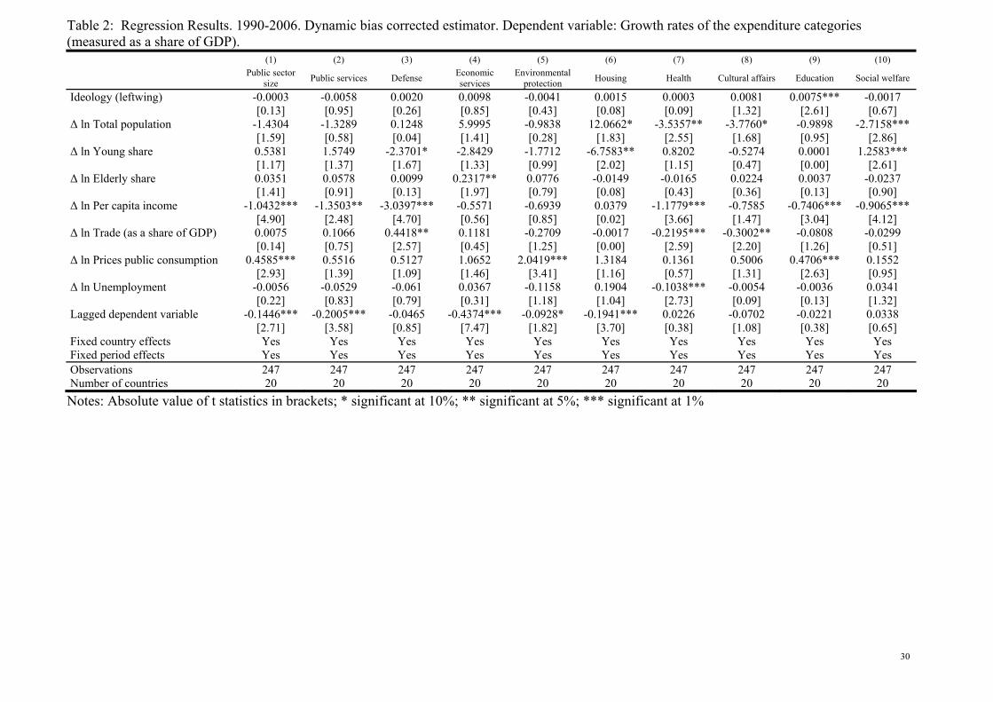
Table 2 provides the results relating to the panel from 1990 to 2006. The results

corroborate my previous findings, that parties did not influence overall government spending

(column 1) and also did not significantly influence the budget composition. Leftwing

governments, however, increased spending on “Education”. The coefficient of the ideology

variable does not turn out to be statistically significant across all other specifications. Real per

capita GDP again emerges as the most important control variable indicating negative

elasticities in the interval between about 1 and even 3 with respect to expenditures on

“Defense” (column 3).

5.2 Robustness of the results

I checked the robustness of the results in several ways. First, I will discuss alternative

econometric specifications of the base-line model in growth rates using somewhat different

control variables and estimation procedures. The previous regressions included trade as a

share of GDP, as it is common in the related literature. Following Dreher (2006) and Dreher

et al. (2008a, 2008b), globalization is a multi-faceted concept that cannot be captured by a

single economic indicator such as international trade, foreign direct investments or capital

account restrictions. Therefore, for a robustness check, I have replaced the explanatory

variable trade-openness by the KOF index of globalization (version 2008) which has been

available till 2005. The demographic change could also be considered by the share of the

working population. I have therefore replaced the shares of the young and the old by

population aged between 15 and 64 as share of total population. To control for

contemporaneous correlation across the countries I have applied panel corrected standard

errors according to Beck and Katz (1996). I have also tested for the existence of arbitrary

serial correlation applying the Wooldridge test (Wooldridge 2002: 176-177) in the static panel

17

data model. The test implies the existence of arbitrary serial correlation in the sample 1970-

1997 for expenditures on “Defense”, “Housing”, and “Social Welfare” and in the sample

1990-2006 for “Public Services”, “Defense”, “Economic Affairs” and “Education”.

Consequently, I have applied heteroskedastic and autocorrelation consistent (HAC) Newey-

West type (Newey and West 1987, Stock and Watson 2008) standard errors and variance-

covariance estimates. The inferences with respect to the influence of government ideology on

the budget composition, however, are not affected (results not shown).

The reported effects could depend on idiosyncratic circumstances in the individual

countries. I therefore test whether the results are sensitive to the inclusion/exclusion of

particular countries. Regarding the first dataset, the influence of the ideology variable on

public services somewhat declines when New Zealand and the USA are excluded. Regarding

the second dataset from 1990 to 2006, excluding Norway, the UK and the USA weakens the

influence of the ideology variable on education spending. When Germany is excluded,

however, the impact of the ideology variables increases.

The results could also depend on the chosen government ideology indicator by

Potrafke (2009a). To rule out this possibility, alternative government ideology indicators can

be used, such as the one by Bjørnskov (2005, 2008a). Hence for robustness checks, I have

employed the recent government ideology indicator by Bjørnskov (2008b) which has been

available till 2004. Bjornskov’s (2008b) index refers to the Henisz (2000) database on

political outcomes since the 19th century, and the general approach to measuring political

ideology follows along the lines of Bjørnskov (2005b, 2008a). However, as compared to the

index employed in Bjørnskov (2005b, 2008a), the Bjørnskov (2008b) index “takes the social

democrat party in a given country as an internationally comparable anchor around which other

parties are placed on a five-point scale (-1; -.5; 0; .5; 1) from left to right” (Bjørnskov 2008b:

5). The ideology scores of each government party are weighed with their relative share of all

government party seats in parliament in order to consider differing degrees of influence on

18

government policy. This procedure addresses the ideological position of the government and

the parliament. Employing this index does not change the inferences.

It is conceivable that the estimates change when government ideology is lagged. I have

therefore replaced the government ideology variable in period t by its lagged values in the

years t-1, t-2, t-3 and t-4. The results show that the estimated influence of government

ideology on “Public Services” over the period 1970-1997 and on “Education” over the period

1990-2006 are robust: while government ideology in period t-1 still has a significant and

positive influence, ideology lagged by four years turns out to have a significant and negative

influence. Against the background that legislative periods usually last four years and

governments frequently change, this is a reasonable finding.

In my base-line econometric model, I have regressed the growth rate of the

expenditure categories on the level of government ideology. This specification reveals that

incumbents change the budget composition incrementally. An alternative specification is an

error correction model (ECM) that allows distinguishing between long-run and short-run

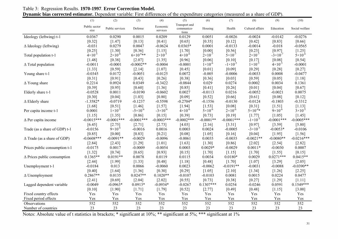
effects of government ideology. I have therefore also estimated an ECM.17 The regression

results reported in Tables 3 (dynamic bias corrected estimator) illustrate that government

ideology hardly influenced the budget composition in the period 1970-1997. The ideology

variables in column (2) still have a positive sign but fail statistical significance at

conventional levels. The first difference of ideology variable in levels is statistically

significant at the 10% level in column (5) indicating that leftwing government somewhat

increased spending for “Transport and communications” in the short run. The results are

however somewhat sensitive to the estimation procedure: the long-run ideology-induced

effects on public services is statistically significant at the 1% level when panel corrected

standard errors and at the 5% level when FGLS with heteroskedastic and autocorrelation

17

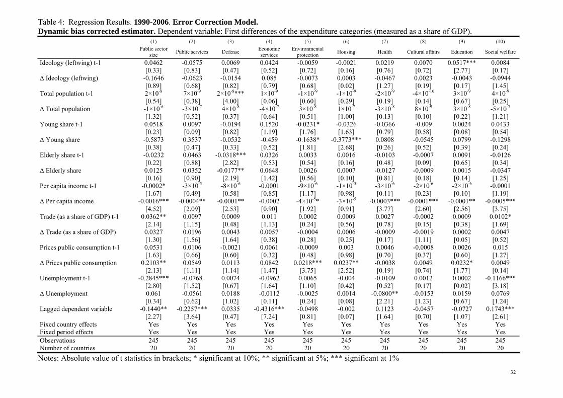
In an ECM, the first differences of the expenditure categories are regressed on the first differences of the explanatory variables (short-run effect) and the lagged levels of the explanatory variables (long-run effect). I have estimated ECM using Bruno´s estimator, panel corrected standard errors and FGLS with heteroskedastic and autocorrelation consistent standard errors.

19

consistent standard errors are used. The results in Table 4 show that in the long-run,

expenditures for “Education” in the period 1990-2006 were higher under leftwing

governments. The coefficient of the ideology variable is statistically significant at the 1%

level. This result is however also somewhat sensitive to the estimation procedure because the

effect does not turn out to be statistically significant when panel corrected standard errors and

FGLS with heteroskedastic and autocorrelation consistent standard errors are used.

A caveat applying to all panel data models concerns potential endogeneity of the

explanatory variables. In my analysis, it is, however, not reasonable to believe that

government ideology is influenced by budget composition. Moreover, good instrumental

variables for government ideology are not available. It is important to note in particular that

instrumenting ideology with the help of lagged government ideology would not be reasonable

because ideology is a highly persistent variable.

In several federal states, the federal governments are not responsible for expenditures

on education such as schools and universities. Education policy is a matter of the state

governments. For this reason, I have excluded the federal states Austria, Germany, Canada

and the United States to check the robustness of the ideology-induced effect on education

expenditures in the period 1990-2006. Inferences do not change at all (I have used several

estimation techniques): leftwing governments increased education expenditures in the period

1990-2006. Government ideology did not influence education spending in the 1970-1997 sub

sample, when the federal states (Austria, Germany, Canada, Switzerland and the United

States) are excluded.

6. Conclusions

Government ideology has had a rather weak influence on the composition and the size

of governments’ budgets in OECD countries. Leftist governments, however, increased

spending on “Public Services” in the period 1970-1997 and on “Education” in the period

20

1990-2006. The lack of ideology-induced fiscal policy making confirms related empirical

findings that government ideology hardly concerned budgetary affairs in the last two decades,

but ideology-induced effects can be identified in non-budgetary affairs. For example,

government ideology has had a strong influence on political alignment with the United States:

leftwing governments were less sympathetic to US positions (Potrafke 2009b). The distinctly

different alignments of leftist and rightwing governments with the United States reflect

sources of ideological association that transcend issues of economic policy. Future research

may therefore investigate further how government ideology influences non-budgetary affairs

and also issues that do not relate the economy such as international relations or migration

policy (see, e.g., Schneider and Urpelainen 2010).

Globalization could counteract partisan politics, or even restricts politicians’ options

or ability to maneuver. Leftist governments are, for example, believed to have lost the ability

to implement their preferred policies such as direct income redistribution. The available

empirical evidence for the OECD countries, however, does not indicate that globalization has

counteracted partisan politics (Potrafke 2009a) and that globalization demolishes the welfare

state. The results presented by Dreher et al. (2008a) suggest, for example, that globalization

did not affect budget composition, whereas Busemeyer (2009b) finds a negative association

between trade-openness and public spending in OECD countries (see Dreher et al. 2008b;

Schulze and Ursprung 1999, and Ursprung 2008 for surveys of the literature on the nexus

between globalization and the welfare state).

Why is it that in times of declining electoral cohesion education policy appears to

emerge as a central policy field that attracts attention of various societal groups? Equality of

opportunity has always been a concern in the political debate but has for a long time been

overshadowed by equality of distribution. Since direct income redistribution is no longer

feasible, equality of opportunity takes a centre stage position. As far as education policy is

concerned, it is well known that the family background has an important influence on the

21

return to education. Even university students with a minority background and from schools

located in economically disadvantaged areas, are likely to be academically less successful

(Betts and Morrell 1999). For this reason, unprivileged citizens are in favor of higher public

education expenditures with the consequence that leftist parties will focus on this policy field

to gratify their original constituencies and, for example, try to reduce income inequality (on

distributional effects of public education expenditures see, for example, Sylwester 2002 and

Tsakloglou and Antoninis 1999). In the course of trying to become more broadly-based, leftist

parties also vie to attract middle-class voters who also prefer higher public education

spending. Working middle-class parents are in favor of publicly provided full-time child care

and university education. Core constituents of rightwing parties will support high public

education expenditures if they can be convinced that such a policy generates higher tax

revenues and lower social transfers in the future.

In contrast to direct income redistribution via the welfare system (social security,

public health system or unemployment benefits), the entire electorate tends to benefit from a

higher education level of the society. Leftwing parties that have moved to the right are

therefore likely to focus exactly on education policy to attract voters from all societal groups:

to be sure, their traditional constituency profits most from higher public education

expenditures, but education policy is not likely to alienate other potential voters. Rightwing

governments do not entirely adjust because they still favor private alternatives. In conclusion,

my results suggest that education policy may well play a significant role in future policy

debates.

Acknowledgements I thank Georgios Chortareas, Heinrich Ursprung, two anonymous referees and the participants of the World Meeting of the Public Choice Society 2007 in Amsterdam for helpful comments and suggestions on earlier versions of the paper. Jakob Schwab and Carl Maier have provided excellent research assistance.

22

References Alesina, A. (1987). Macroeconomic policy in a two-party system as a repeated game.

Quarterly Journal of Economics 102, 651-678.

Alesina, A., Roubini, N., & Cohen G.D. (1997). Political cycles and the macroeconomy.

The MIT Press, Cambridge.

Alt, J.E., Lassen, D.D. (2006). Fiscal transparency, political parties, and debt in OECD

countries. European Economic Review 50, 1403-1439.

Angelopoulos, K. & Economides, G. (2008). Fiscal policy, rent seeking, and growth under

electoral uncertainty: theory and evidence from the OECD.

Canadian Journal of Economics 41, 1375-1405.

Ansell, B.W. (2008). University challenges explaining institutional change in higher

education. World Politics 60, 189-230.

Arellano, M., & Bond, S. (1991). Some Tests of Specification for Panel Data: Monte Carlo

Evidence and an Application to Employment Equations. Review of Economic Studies

58, 277–297.

Beck, N., & Katz, J.N. (1996). Nuisance vs. substance: Specifying and estimating time-series

cross section models. Political Analysis 6, 1-36.

Behr, A. (2003). A comparison of dynamic panel data estimators: Monte Carlo evidence and

an application to the investment function.

Discussion paper 05/03, Economic Research Centre of the Deutsche Bundesbank.

Bel., G., & Elias-Moreno, F. (2009). Institutional determinants of military spending.

Working Paper 2009/22, Research Institute of Applied Economics, Barcelona.

Bercoff, J. J., & Meloni, O. (2009). Federal budget allocation in an emergent democracy:

evidence from Argentina. Economics of Governance 10, 65-83.

Betts, J.R., & Morrell, D. (1999). The determinants of undergraduate grade point average:

The relative importance of family background, high school resources, and peer group

effects. Journal of Human Resources 34, 268-293.

Bierbrauer, F. (2009). Optimal income taxation and public good provision with endogenous

interest groups. Journal of Public Economic Theory 11, 311-342.

Bjørnskov, C. (2005). Does political ideology affect economic growth?

Public Choice 123, 133-146.

Bjørnskov, C. (2008a). The growth-inequality association: government ideology matters.

Journal of Development Economics 87, 300-308.

23

Bjørnskov, C. (2008b). Political ideology and the structure of national accounts in the Nordic

Countries, 1950-2004. Paper presented at the annual meeting of the European Public

Choice Society, Jena 27-30 March 2008.

Bjørnskov, C., & Potrafke, N. (2011a). Politics and privatization in Central and Eastern

Europe: a panel data analysis. Economics of Transition, forthcoming.

Bjørnskov, C., & Potrafke, N. (2011b). Political ideology and economic freedom across

Canadian provinces. Eastern Economic Journal, forthcoming.

Bloom, D., Canning, D., Mansfield, R.K., & Moore, M. (2007). Demographic change, social

security systems, and savings. Journal of Monetary Economics 54, 92-114.

Blundell, R.W., & Bond, S.R. (1998). Initial conditions and moment restrictions in dynamic

Panel data models. Journal of Econometrics 87, 115–143.

Boix, C. (1997). Political parties and the supply side of the economy: The provision of

Physical and human capital in advanced economies, 1960-90.

American Journal of Political Science 1997 41, 814-845.

Boix, C. (1998). Political parties, growth and equality – Conservative and social democratic

economic strategies in the world economy. Cambridge, Cambridge University Press.

Bräuninger, T. (2005). A partisan model of government expenditure.

Public Choice 125, 409-429.

Bruno, G.S.F. (2005a). Approximating the bias of the LSDV estimator for dynamic

Unbalanced panel data models. Economics Letters 87, 361-366.

Bruno, G.S.F. (2005b). Estimation and inference in dynamic unbalanced panel data models

With a small number of individuals. Stata Journal 5, 473-500.

Budge, I., Keman, H., & Woldendorp, J. (1993). Political data 1945-1990. Party government

in 20 democracies. European Journal of Political Research 24, 1-119.

Busemeyer, M.R. (2007). Determinants of public education spending in 21 OECD

democracies, 1980-2001. Journal of European Public Policy 14, 582-610.

Busemeyer, M.R. (2009a). Social democrats and the new partisan politics of public

Investment in education. Journal of European Public Policy 16, 107-126.

Busemeyer, M.R. (2009b). From myth to reality: globalization and public spending in OECD

countries revisited. European Journal of Political Research 48, 455-482.

Calcagno, P.T., & Escaleras, M. (2007). Party alternation, divided government, and fiscal

performance within US states. Economics of Governance 8, 111-128.

Congleton, R.D., & Bose, F. (2010). The rise of the modern welfare state, ideology,

Institutions and income security: analysis and evidence. Public Choice 144, 535-555.

24

Correa, H., & Kim, J.-W. (1992). A causal analysis of defence expenditures of the USA and

The USSR. Journal of Peace Research 29, 161-174.

Cremer, H., De Donder, P., & Gahvari, F. (2008). Political competition within and between

parties: an application to environmental policy.

Journal of Public Economics 92, 532-547.

De Donder, P., & Hindriks, J. (2007). Equilibrium social insurance with policy-motivated

parties. European Journal of Political Economy 23, 624-640.

Drazen, A., & Eslava, M. (2010). Electoral manipulation via voter-friendly spending:

Theory and evidence. Journal of Development Economics 92, 39-52.

Dreher, A., (2006). Does globalization affect growth? Evidence from a new index of

globalization. Applied Economics 38, 1091-1110.

Dreher, A., Sturm, J.-E., & Ursprung, H.W. (2008a). The impact of globalization on the

composition of government expenditures: Evidence from panel data.

Public Choice 134, 263-292.

Dreher, A., Gaston, N., & Martens, P. (2008b). Measuring globalization – Gauging its

consequences. Berlin, Springer.

Gemmell, N., Kneller, R., & Sanz, I., (2008). Foreign investment, international trade and the

size and structure of public expenditures.

European Journal of Political Economy 24, 151-171.

Heckelman, J. C. (2002). Variable rational partisan business cycles: theory and some

evidence. Canadian Journal of Economics 35, 568-585.

Henisz, W. (2000). The institutional environment for growth.

Economics and Politics 12, 1-31.

Hibbs, D.A. Jr. (1977). Political parties and macroeconomic policy. American Political

Science Review 71, 1467-1487.

Hicks, A.M., & Swank, D. (1992). Politics, institutions and welfare spending in

industrialized democracies, 1960-82.

American Political Science Review 86, 658-674.

Huber, E., & Stephens, J.D. (2001). Development and crisis of the welfare state. Parties

and policies in global markets. Chicago and London: University of Chicago Press.

Immergut, E.M. (1992). Health politics – Interests and institutions in Western Europe.

Cambridge, Cambridge University Press.

Iversen, T., & Stephens, J.D. (2008). Partisan politics, the welfare state, and three worlds of

human capital formation. Comparative Political Studies 41, 600-637.

25

Jensen, C. (2010). Issue compensation and right-wing social spending.

European Journal of Political Research 49, 282-299.

Jensen, C. (2011a). Marketization via compensation: health care and the politics of the right

In advanced industrialized nations. British Journal of Political Science, forthcoming.

Jensen, C. (2011b). Determinants of welfare service provision after the Golden Age.

International Journal of Social Welfare, forthcoming.

Jensen, C. (2011c). Capitalist systems, de-industrialization, and the politics of public

education. Comparative Political Studies, forthcoming.

Johansen, K., Mydland, Ø., & B. Strøm (2007). Politics in wage setting: does government

colour matter? Economics of Governance 8, 95-109.

Katsimi, M., & Sarantides, V. (2010). Do elections affect the composition of fiscal policy?

CESifo Working Papers No. 2908, Munich.

Kittel, B., & Obinger, H. (2003). Politicial parties, institutions, and the dynamics of social

expenditure in times of austerity. Journal of European Public Policy 10, 20-45.

Kneebone, R.D., & McKenzie, K. J. (2001). Electoral and partisan cycles in fiscal policy:

an examination of Canadian provinces.

International Tax and Public Finance 8, 753-774.

Lago-Peñas, I. & Lago-Peñas, S. (2009). Does the nationalization of party systems affect the

composition of public spending? Economics of Governance 10, 85-98.

Lange, P., & Garrett, G. (1985). The politics of growth: strategic interaction and economic

performance in advanced industrialized democracies, 1974-1980.

Journal of Politics 47, 792-827.

Laurency, P., & Schindler, D. (2010). Why green parties should fear successful international

climate agreements. TWI Discussion Papers No. 56, Kreuzlingen.

Merzyn, W., & Ursprung, H.W. (2005). Voter support for privatizing education: evidence

self-interest and ideology. European Journal of Political Economy 25, 33-58.

Newey, W.K., & West, K.D. (1987). A simple, positive semi-definite, heteroskedasticity and

autocorrelation consistent covariance matrix. Econometrica 55, 703-708.

Nincic, M., & Cusack, T.R. (1979). The political economy of US military spending.

Journal of Peace Research 16, 101-115.

Nordhaus, W. D. (1975). The political business cycle.

Review of Economic Studies 42, 169-190.

26

Oberndorfer, U., & Steiner, V. (2007). Generationen- oder Parteienkonflikt? Eine

empirische Analyse der deutschen Hochschulausgaben.

Perspektiven der Wirtschaftspolitik 8, 165-183.

OECD (2008). Main Economic Indicators. Paris.

Ono,T. (2009). The political economy of environmental and social security policies:

the role of environmental lobbying. Economics of Governance 10, 261-296.

Pierson, P. (1996). The new politics of the welfare state. World Politics, 48, 143–179.

Pierson, P. (2001). Post-industrial pressures on the mature welfare states. In Pierson, P. (Eds.),

The new politics of the welfare state. Oxford: Oxford University Press, 80–104.

Potrafke, N. (2009a). Did globalization restrict partisan politics? An empirical evaluation of

social expenditures in a panel of OECD countries. Public Choice 140, 105-124.

Potrafke, N. (2009b). Does government ideology influence political alignment with the U.S.?

An empirical analysis of voting in the UN General Assembly.

Review of International Organizations 4, 245-268.

Potrafke, N. (2010a). The growth of public health expenditures in OECD countries: do

government ideology and electoral motives matter?

Journal of Health Economics 29, 797-810.

Potrafke N (2010b) Does government ideology influence deregulation of product markets?

Empirical evidence from OECD countries. Public Choice 143, 135-155.

Potrafke, N. (2010c). Ideology and cultural policy.

TWI Discussion Papers No. 49, Kreuzlingen.

Potrafke, N. (2011a). Public expenditures on education and cultural affairs in the West

German states: does government ideology influence the budget composition?

German Economic Review 12, 124-145.

Potrafke, N. (2011b). Political cycles and economic performance in OECD countries:

empirical evidence from 1951-2006. Public Choice, forthcoming.

Rogoff, K & Sibert, A. (1988). Elections and macroeconomic policy cycles.

Review of Economic Studies 55, 1-16.

Roodman, D. (2009). A note on the theme of too many instruments.

Oxford Bulletin of Economics and Statistics 71, 135-158.

Roodman, D. (2006). How to do xtabond2: An introduction to “Difference” and “System”

GMM in Stata. Center for Global Development. Working Paper 103.

Rose, R. (1990). Inheritance before choice in public policy.

Journal of Theoretical Politics 2, 263-291.

27

Sakamoto, T. (2008). Economic policy and performance in industrial democracies – party

governments, central banks and the fiscal-monetary policy mix. Routledge,

London and New York.

Sanz, I., & Velázquez, F. (2007). The role of aging in the growth of government and social

welfare spending in the OECD.

European Journal of Political Economy 23, 917-931.

Schmidt, M.G. (2007). Testing the retrenchment hypothesis: education spending, 1960-2002.

In Castles, F.G. (eds.). The disappearing state? Retrenchment realities in an age of

globalization. Celtenham: Edward Elgar, 159-183.

Schneider, C., & Urpelainen, J. (2010). Partisan waves in international coorperation.

Working Paper, University of California, San Diego.

Schulze, G.G., & Rose, A. (1998). Public orchestra funding in Germany – an empirical

investigation. Journal of Cultural Economics 22, 227-247.

Schulze, G.G., & Ursprung, H.W. (1999). Globalisation of the economy and the nation state.

World Economy 22, 295-352.

Schulze, G.G., & Ursprung, H.W. (2000). La donna e mobile – or is she? Voter

preferences and public support for the performing arts.

Public Choice 102, 131-149.

Shelton, C.A. (2007). The size and composition of government expenditure.

Journal of Public Economics 91, 2230-2260.

Shi, M. & Svensson, J. (2006). Political budget cycles: do they differ across countries and

why? Journal of Public Economics 90, 1367-1389.

Stock, J.H., & Watson, M.W. (2008). Heteroskedasticity-robust standard errors for

fixed-effects panel-data regression. Econometrica 76, 155-174.

Sylwester, K. (2002). Can education expenditures reduce income inequality?

Economics of Education Review 21, 43-52.

Tavares, J. (2004). Does right or left matter? Cabinets, credibility and fiscal adjustment.

Journal of Public Economics 88, 2447-2468.

Tepe, M. & Vanhuysse, P. (2009a). Educational business cycles – The political economy of

teacher hiring across German states, 1992-2004. Public Choice 139, 61-82.

Tepe, M. & Vanhuysse, P. (2009b). Are aging OECD welfare states on the path to

gerontocracy? Evidence from 18 democracies, 1980-2002.

Journal of Public Policy 29, 1-28.

28

Tepe, M. & Vanhuysse, P. (2010). Who cuts back and when? The politics of delays in social

expenditure cutbacks, 1980-2005. West European Politics 33, 1214-1240.

Tridimas, G. (2001). The economics and politics of the structure of public expenditure.

Public Choice 106, 299-316.

Tsakloglou, P., & Antoninis. M. (1999). On the distributional impact of public education:

evidence from Greece. Economics of Education Review 18, 439-452.

Ursprung, H. W. (2008). Globalisation and the welfare state. In Durlauf, S. N. & Blume, L.

(eds.). The New Palgrave Dictionary of Economics, Second edition.

Köln: Palgrave Macmillan.

Vergne, C. (2009). Democracy, elections and allocation of public expenditures in developing

countries European Journal of Political Economy 25, 63-77.

Woldendorp, J., Keman, H., & Budge, I. (1998). Party government in 20 democracies: an

update 1990-1995. European Journal of Political Research 33, 125-164.

Woldendorp, J., Keman, H., & Budge, I. (2000). Party government in 48 democracies

1945-1998: composition, duration, personnel.

Dordrecht, Kluwer Academic Publishers.

Wooldridge, J. M. (2002). Econometric analysis of cross section and panel data.

Cambridge, MIT Press.

World Bank (2007). World Development Indicators. Washington, D. C.

World Bank (2008). World Development Indicators. Washington, D. C.

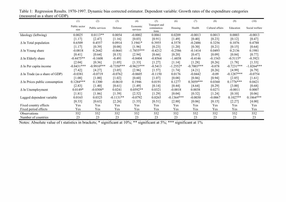
Table 1: Regression Results. 1970-1997. Dynamic bias corrected estimator. Dependent variable: Growth rates of the expenditure categories (measured as a share of GDP).

(1) (2) (3) (4) (5) (6) (7) (8) (9) (10)

Public sector size Public services Defense Economic

services

Transport and communica-

tions Housing Health Cultural affairs Education Social welfare

Ideology (leftwing) 0.0025 0.0113** 0.0054 -0.0002 0.0061 0.0209 -0.0013 0.0013 0.0003 -0.0013 [1.17] [2.47] [1.16] [0.03] [0.91] [1.49] [0.40] [0.23] [0.12] [0.47] ∆ ln Total population 0.6509 0.4557 0.0914 3.1941* 0.3955 4.3578 -0.2486 0.3256 0.1076 0.4788 [1.17] [0.39] [0.08] [1.96] [0.23] [1.20] [0.30] [0.21] [0.15] [0.64] ∆ ln Young share -0.0818 0.2642 -0.0641 -1.7855*** -0.4212 -0.2586 -0.1414 0.0493 0.2136 0.1981 [0.41] [0.64] [0.15] [2.94] [0.66] [0.20] [0.47] [0.09] [0.84] [0.77] ∆ ln Elderly share -0.4475** -0.1608 -0.491 -0.8404 -0.8564 -1.6038 -0.4146 -0.1543 -0.5115* -0.3921 [2.04] [0.36] [1.05] [1.33] [1.27] [1.14] [1.28] [0.26] [1.78] [1.33] ∆ ln Per capita income -0.8431*** -0.9910*** -0.7350*** -0.9623*** -0.5413 -1.2552* -0.7003*** -0.078 -0.7231*** -1.0264*** [7.42] [4.27] [3.05] [2.96] [1.57] [1.74] [4.21] [0.26] [4.99] [6.79] ∆ ln Trade (as a share of GDP) -0.0381 -0.0719 -0.0762 -0.0605 -0.1150 0.0176 -0.0442 -0.09 -0.1287*** -0.0754 [1.08] [1.00] [1.02] [0.60] [1.07] [0.08] [0.86] [0.94] [2.85] [1.61] ∆ ln Prices public consumption 0.1284*** 0.1300 -0.0610 0.1946 0.0191 0.1277 0.3059*** 0.0360 0.1776*** 0.0421 [2.83] [1.40] [0.61] [1.49] [0.14] [0.44] [4.64] [0.29] [3.00] [0.68] ∆ ln Unemployment 0.0149* -0.0308* 0.0241 0.0592** 0.0321 -0.0018 0.0038 0.0271 -0.0011 0.0007 [1.81] [1.86] [1.39] [2.52] [1.29] [0.04] [0.32] [1.24] [0.10] [0.06] Lagged dependent variable 0.0165 0.0325 -0.1131** -0.0792 0.0265 -0.1364*** -0.0030 -0.0067 0.1027** 0.1864*** [0.33] [0.63] [2.26] [1.55] [0.51] [2.88] [0.06] [0.15] [2.27] [4.00] Fixed country effects Yes Yes Yes Yes Yes Yes Yes Yes Yes Yes Fixed period effects Yes Yes Yes Yes Yes Yes Yes Yes Yes Yes Observations 552 552 552 552 552 552 552 552 552 552 Number of countries 23 23 23 23 23 23 23 23 23 23 Notes: Absolute value of t statistics in brackets; * significant at 10%; ** significant at 5%; *** significant at 1%

30

Table 2: Regression Results. 1990-2006. Dynamic bias corrected estimator. Dependent variable: Growth rates of the expenditure categories (measured as a share of GDP).

(1) (2) (3) (4) (5) (6) (7) (8) (9) (10)

Public sector size Public services Defense Economic

services Environmental

protection Housing Health Cultural affairs Education Social welfare

Ideology (leftwing) -0.0003 -0.0058 0.0020 0.0098 -0.0041 0.0015 0.0003 0.0081 0.0075*** -0.0017 [0.13] [0.95] [0.26] [0.85] [0.43] [0.08] [0.09] [1.32] [2.61] [0.67] ∆ ln Total population -1.4304 -1.3289 0.1248 5.9995 -0.9838 12.0662* -3.5357** -3.7760* -0.9898 -2.7158*** [1.59] [0.58] [0.04] [1.41] [0.28] [1.83] [2.55] [1.68] [0.95] [2.86] ∆ ln Young share 0.5381 1.5749 -2.3701* -2.8429 -1.7712 -6.7583** 0.8202 -0.5274 0.0001 1.2583*** [1.17] [1.37] [1.67] [1.33] [0.99] [2.02] [1.15] [0.47] [0.00] [2.61] ∆ ln Elderly share 0.0351 0.0578 0.0099 0.2317** 0.0776 -0.0149 -0.0165 0.0224 0.0037 -0.0237 [1.41] [0.91] [0.13] [1.97] [0.79] [0.08] [0.43] [0.36] [0.13] [0.90] ∆ ln Per capita income -1.0432*** -1.3503** -3.0397*** -0.5571 -0.6939 0.0379 -1.1779*** -0.7585 -0.7406*** -0.9065*** [4.90] [2.48] [4.70] [0.56] [0.85] [0.02] [3.66] [1.47] [3.04] [4.12] ∆ ln Trade (as a share of GDP) 0.0075 0.1066 0.4418** 0.1181 -0.2709 -0.0017 -0.2195*** -0.3002** -0.0808 -0.0299 [0.14] [0.75] [2.57] [0.45] [1.25] [0.00] [2.59] [2.20] [1.26] [0.51] ∆ ln Prices public consumption 0.4585*** 0.5516 0.5127 1.0652 2.0419*** 1.3184 0.1361 0.5006 0.4706*** 0.1552 [2.93] [1.39] [1.09] [1.46] [3.41] [1.16] [0.57] [1.31] [2.63] [0.95] ∆ ln Unemployment -0.0056 -0.0529 -0.061 0.0367 -0.1158 0.1904 -0.1038*** -0.0054 -0.0036 0.0341 [0.22] [0.83] [0.79] [0.31] [1.18] [1.04] [2.73] [0.09] [0.13] [1.32] Lagged dependent variable -0.1446*** -0.2005*** -0.0465 -0.4374*** -0.0928* -0.1941*** 0.0226 -0.0702 -0.0221 0.0338 [2.71] [3.58] [0.85] [7.47] [1.82] [3.70] [0.38] [1.08] [0.38] [0.65] Fixed country effects Yes Yes Yes Yes Yes Yes Yes Yes Yes Yes Fixed period effects Yes Yes Yes Yes Yes Yes Yes Yes Yes Yes Observations 247 247 247 247 247 247 247 247 247 247 Number of countries 20 20 20 20 20 20 20 20 20 20 Notes: Absolute value of t statistics in brackets; * significant at 10%; ** significant at 5%; *** significant at 1%

31

Table 3: Regression Results. 1970-1997. Error Correction Model. Dynamic bias corrected estimator. Dependent variable: First differences of the expenditure categories (measured as a share of GDP).

(1) (2) (3) (4) (5) (6) (7) (8) (9) (10)

Public sector size Public services Defense Economic

services

Transport and communica-

tions Housing Health Cultural affairs Education Social welfare

Ideology (leftwing) t-1 0.0367 0.0290 0.0015 0.0209 0.0129 0.0051 -0.0026 -0.0024 -0.0142 -0.0276 [0.32] [1.47] [0.13] [0.41] [0.65] [0.35] [0.12] [0.42] [0.83] [0.66] ∆ Ideology (leftwing) -0.031 0.0279 0.0047 -0.0624 0.0365* 0.0001 -0.0133 -0.0014 -0.018 -0.0565 [0.25] [1.30] [0.36] [1.15] [1.70] [0.00] [0.56] [0.23] [0.97] [1.25] Total population t-1 4×10-5 2×10-6 6×10-6** 2×10-5 4×10-6 2×10-7 5×10-7 2×10-7 -3×10-7 5×10-6 [1.48] [0.38] [2.07] [1.35] [0.96] [0.06] [0.10] [0.17] [0.08] [0.54] ∆ Total population -0.0011 -0.0001 -0.0002** -0.0004 -0.0001 1×10-6 -1×10-5 1×10-5 4×10-5 -0.0001 [1.33] [0.59] [2.14] [1.07] [0.45] [0.01] [0.09] [0.29] [0.28] [0.27] Young share t-1 -0.0345 0.0172 -0.0051 -0.0125 0.0072 -0.005 -0.0006 -0.0033 0.0008 -0.0477 [0.31] [0.91] [0.43] [0.26] [0.38] [0.36] [0.03] [0.59] [0.05] [1.18] ∆ Young share 0.2214 0.0924 0.0349 -0.3422 -0.0844 0.029 0.0274 0.0002 0.0034 0.1361 [0.39] [0.95] [0.60] [1.36] [0.85] [0.41] [0.26] [0.01] [0.04] [0.67] Elderly share t-1 -0.0528 0.0011 -0.0190 -0.0602 0.0027 -0.0113 0.0216 -0.0052 -0.0021 0.0075 [0.30] [0.04] [1.03] [0.80] [0.09] [0.52] [0.66] [0.61] [0.08] [0.12] ∆ Elderly share -1.3582* -0.0719 -0.1237 -0.5598 -0.2704* -0.1556 -0.0130 -0.0124 -0.1803 -0.3312 [1.68] [0.51] [1.46] [1.57] [1.94] [1.53] [0.08] [0.31] [1.51] [1.13] Per capita income t-1 0.0001 1×10-5 -5×10-6 -3×10-6 4×10-6 5×10-6 2×10-6 5×10-6* 9×10-6 3×10-5 [1.15] [1.35] [0.86] [0.15] [0.39] [0.73] [0.19] [1.77] [1.05] [1.45] ∆ Per capita income -0.0015*** -0.0001*** -0.0001*** -0.0003*** -0.0002*** -0.0001** -0.0001*** -1×10-5 -0.0001*** -0.0005*** [6.45] [2.75] [2.71] [2.73] [4.03] [2.16] [3.31] [0.97] [3.59] [5.80] Trade (as a share of GDP) t-1 -0.0156 9×10-6 -0.0016 0.0016 0.0003 0.0024 -0.0005 -3×10-5 -0.0053* -0.0106 [0.85] [0.00] [0.83] [0.21] [0.08] [1.05] [0.16] [0.04] [1.95] [1.56] ∆ Trade (as a share of GDP) -0.0608*** -0.0091** -0.0029 -0.0096 -0.0061 0.0035 -0.0035 -0.0021** -0.0080** -0.0216*** [2.84] [2.43] [1.29] [1.01] [1.63] [1.30] [0.86] [2.02] [2.54] [2.82] Prices public consumption t-1 -0.0175 0.0017 -0.0009 -0.0054 0.0003 0.0029* -0.0029 0.0011* -0.0030 0.0007 [1.32] [0.74] [0.65] [0.93] [0.15] [1.70] [1.15] [1.70] [1.55] [0.15] ∆ Prices public consumption 0.1365** 0.0191** 0.0078 0.0119 0.0115 0.0034 0.0180* 0.0029 0.0271*** 0.0415** [2.44] [1.99] [1.33] [0.48] [1.18] [0.48] [1.70] [1.07] [3.29] [2.05] Unemployment t-1 -0.0184 0.013 0.0066 -0.0060 0.0023 -0.0062 -0.0191** -0.0031 -0.0088 -0.0390** [0.40] [1.64] [1.36] [0.30] [0.29] [1.05] [2.10] [1.34] [1.26] [2.25] ∆ Unemployment 0.2867** 0.0135 0.0247** 0.1020** -0.0107 -0.0103 0.0081 0.0015 0.0224 0.0477 [2.41] [0.69] [2.04] [2.02] [0.55] [0.73] [0.38] [0.27] [1.29] [1.11] Lagged dependent variable -0.0049 -0.0963* 0.0913* -0.0934* -0.0267 0.1307*** 0.0254 -0.0246 0.0591 0.1549*** [0.10] [1.90] [1.71] [1.79] [0.52] [2.77] [0.49] [0.48] [1.15] [3.00] Fixed country effects Yes Yes Yes Yes Yes Yes Yes Yes Yes Yes Fixed period effects Yes Yes Yes Yes Yes Yes Yes Yes Yes Yes Observations 552 552 552 552 552 552 552 552 552 552 Number of countries 23 23 23 23 23 23 23 23 23 23 Notes: Absolute value of t statistics in brackets; * significant at 10%; ** significant at 5%; *** significant at 1%

32

Table 4: Regression Results. 1990-2006. Error Correction Model. Dynamic bias corrected estimator. Dependent variable: First differences of the expenditure categories (measured as a share of GDP).

(1) (2) (3) (4) (5) (6) (7) (8) (9) (10)

Public sector size Public services Defense Economic

services Environmental

protection Housing Health Cultural affairs Education Social welfare

Ideology (leftwing) t-1 0.0462 -0.0575 0.0069 0.0424 -0.0059 -0.0021 0.0219 0.0070 0.0517*** 0.0084 [0.33] [0.83] [0.47] [0.52] [0.72] [0.16] [0.76] [0.72] [2.77] [0.17] ∆ Ideology (leftwing) -0.1646 -0.0623 -0.0154 0.085 -0.0073 0.0003 -0.0467 0.0023 -0.0043 -0.0944 [0.89] [0.68] [0.82] [0.79] [0.68] [0.02] [1.27] [0.19] [0.17] [1.45] Total population t-1 2×10-8 7×10-9 2×10-8*** 1×10-9 -1×10-9 -1×10-9 -2×10-9 -4×10-10 3×10-9 4×10-9 [0.54] [0.38] [4.00] [0.06] [0.60] [0.29] [0.19] [0.14] [0.67] [0.25] ∆ Total population -1×10-6 -3×10-7 4×10-8 -4×10-7 3×10-8 1×10-7 -3×10-8 8×10-9 3×10-8 -5×10-7 [1.32] [0.52] [0.37] [0.64] [0.51] [1.00] [0.13] [0.10] [0.22] [1.21] Young share t-1 0.0518 0.0097 -0.0194 0.1520 -0.0231* -0.0326 -0.0366 -0.009 0.0024 0.0433 [0.23] [0.09] [0.82] [1.19] [1.76] [1.63] [0.79] [0.58] [0.08] [0.54] ∆ Young share -0.5873 0.3537 -0.0532 -0.459 -0.1638* -0.3773*** 0.0808 -0.0545 0.0799 -0.1298 [0.38] [0.47] [0.33] [0.52] [1.81] [2.68] [0.26] [0.52] [0.39] [0.24] Elderly share t-1 -0.0232 0.0463 -0.0318*** 0.0326 0.0033 0.0016 -0.0103 -0.0007 0.0091 -0.0126 [0.22] [0.88] [2.82] [0.53] [0.54] [0.16] [0.48] [0.09] [0.65] [0.34] ∆ Elderly share 0.0125 0.0352 -0.0177** 0.0648 0.0026 0.0007 -0.0127 -0.0009 0.0015 -0.0347 [0.16] [0.90] [2.19] [1.42] [0.56] [0.10] [0.81] [0.18] [0.14] [1.25] Per capita income t-1 -0.0002* -3×10-5 -8×10-6 -0.0001 -9×10-6 -1×10-5 -3×10-6 -2×10-6 -2×10-6 -0.0001 [1.67] [0.49] [0.58] [0.85] [1.17] [0.98] [0.11] [0.23] [0.10] [1.19] ∆ Per capita income -0.0016*** -0.0004** -0.0001** -0.0002 -4×10-5* -3×10-5 -0.0003*** -0.0001*** -0.0001** -0.0005*** [4.52] [2.09] [2.53] [0.90] [1.92] [0.91] [3.77] [2.60] [2.56] [3.75] Trade (as a share of GDP) t-1 0.0362** 0.0097 0.0009 0.011 0.0002 0.0009 0.0027 -0.0002 0.0009 0.0102* [2.14] [1.15] [0.48] [1.13] [0.24] [0.56] [0.78] [0.15] [0.38] [1.69] ∆ Trade (as a share of GDP) 0.0327 0.0196 0.0043 0.0057 -0.0004 0.0006 -0.0009 -0.0019 0.0002 0.0047 [1.30] [1.56] [1.64] [0.38] [0.28] [0.25] [0.17] [1.11] [0.05] [0.52] Prices public consumption t-1 0.0531 0.0106 -0.0021 0.0061 -0.0009 0.003 0.0046 -0.0008 0.0026 0.015 [1.63] [0.66] [0.60] [0.32] [0.48] [0.98] [0.70] [0.37] [0.60] [1.27] ∆ Prices public consumption 0.2103** 0.0549 0.0113 0.0842 0.0218*** 0.0237** -0.0038 0.0049 0.0232* 0.0049 [2.13] [1.11] [1.14] [1.47] [3.75] [2.52] [0.19] [0.74] [1.77] [0.14] Unemployment t-1 -0.2845*** -0.0768 0.0074 -0.0962 0.0065 -0.004 -0.0109 0.0012 0.0002 -0.1166*** [2.80] [1.52] [0.67] [1.64] [1.10] [0.42] [0.52] [0.17] [0.02] [3.18] ∆ Unemployment 0.061 -0.0561 0.0188 -0.0112 -0.0025 0.0014 -0.0800** -0.0153 0.0159 0.0769 [0.34] [0.62] [1.02] [0.11] [0.24] [0.08] [2.21] [1.23] [0.67] [1.24] Lagged dependent variable -0.1440** -0.2257*** 0.0335 -0.4316*** -0.0498 -0.002 0.1123 -0.0457 -0.0727 0.1743*** [2.27] [3.64] [0.47] [7.24] [0.81] [0.07] [1.64] [0.70] [1.07] [2.61] Fixed country effects Yes Yes Yes Yes Yes Yes Yes Yes Yes Yes Fixed period effects Yes Yes Yes Yes Yes Yes Yes Yes Yes Yes Observations 245 245 245 245 245 245 245 245 245 245 Number of countries 20 20 20 20 20 20 20 20 20 20 Notes: Absolute value of t statistics in brackets; * significant at 10%; ** significant at 5%; *** significant at 1%

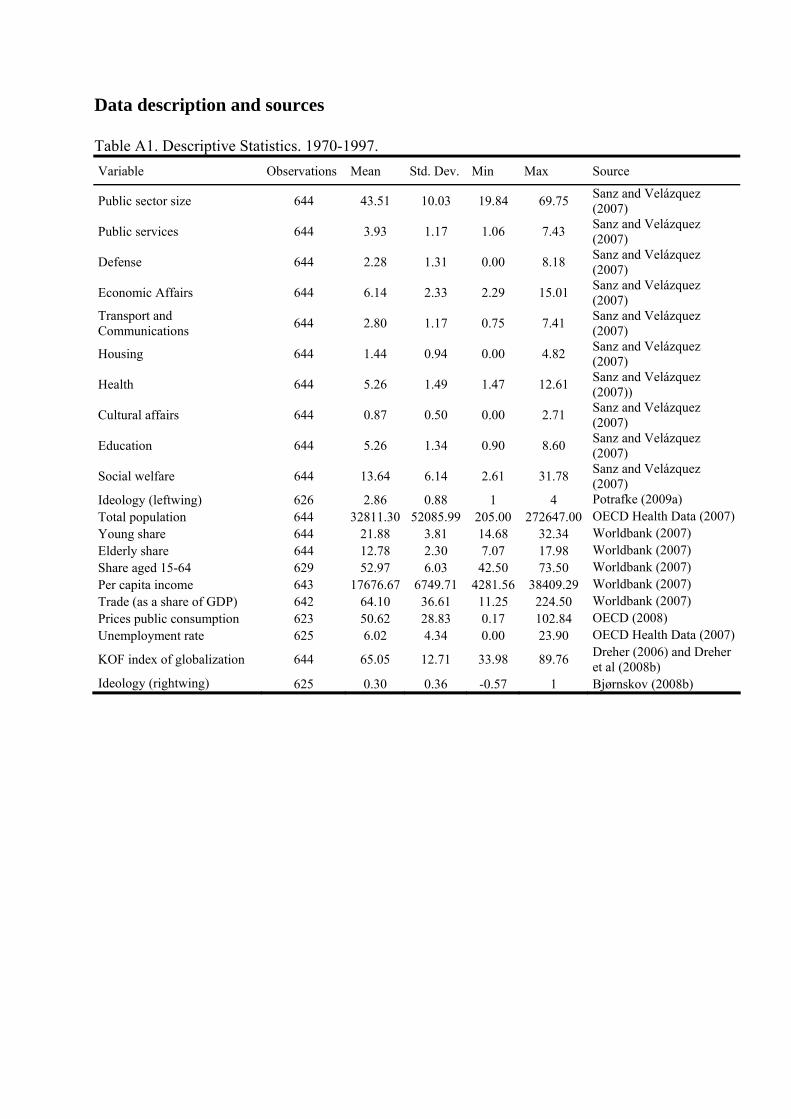
Data description and sources Table A1. Descriptive Statistics. 1970-1997. Variable Observations Mean Std. Dev. Min Max Source

Public sector size 644 43.51 10.03 19.84 69.75 Sanz and Velázquez (2007)

Public services 644 3.93 1.17 1.06 7.43 Sanz and Velázquez (2007)

Defense 644 2.28 1.31 0.00 8.18 Sanz and Velázquez (2007)

Economic Affairs 644 6.14 2.33 2.29 15.01 Sanz and Velázquez (2007)

Transport and Communications 644 2.80 1.17 0.75 7.41 Sanz and Velázquez

(2007)

Housing 644 1.44 0.94 0.00 4.82 Sanz and Velázquez (2007)

Health 644 5.26 1.49 1.47 12.61 Sanz and Velázquez (2007))

Cultural affairs 644 0.87 0.50 0.00 2.71 Sanz and Velázquez (2007)

Education 644 5.26 1.34 0.90 8.60 Sanz and Velázquez (2007)

Social welfare 644 13.64 6.14 2.61 31.78 Sanz and Velázquez (2007)

Ideology (leftwing) 626 2.86 0.88 1 4 Potrafke (2009a) Total population 644 32811.30 52085.99 205.00 272647.00 OECD Health Data (2007)Young share 644 21.88 3.81 14.68 32.34 Worldbank (2007) Elderly share 644 12.78 2.30 7.07 17.98 Worldbank (2007) Share aged 15-64 629 52.97 6.03 42.50 73.50 Worldbank (2007) Per capita income 643 17676.67 6749.71 4281.56 38409.29 Worldbank (2007) Trade (as a share of GDP) 642 64.10 36.61 11.25 224.50 Worldbank (2007) Prices public consumption 623 50.62 28.83 0.17 102.84 OECD (2008) Unemployment rate 625 6.02 4.34 0.00 23.90 OECD Health Data (2007)

KOF index of globalization 644 65.05 12.71 33.98 89.76 Dreher (2006) and Dreher et al (2008b)

Ideology (rightwing) 625 0.30 0.36 -0.57 1 Bjørnskov (2008b)

34

Table A2. Descriptive Statistics. 1990-2006. Variable Observations Mean Std. Dev. Min Max Source

Public sector size 289 46.62 7.01 31.47 65.09 OECD (2008) Public services 289 9.15 2.68 3.61 17.61 OECD (2008) Defense 289 1.67 0.99 0.00 5.64 OECD (2008) Economic Affairs 289 4.72 1.22 2.19 11.10 OECD (2008) Environmental protection 289 0.65 0.35 0.00 1.82 OECD (2008) Housing 289 0.86 0.48 0.15 6.26 OECD (2008) Health 289 6.23 1.03 3.37 8.89 OECD (2008) Cultural affairs 289 1.08 0.59 0.15 3.66 OECD (2008) Education 289 5.72 1.40 2.34 9.55 OECD (2008) Social welfare 289 16.53 5.07 6.60 28.36 OECD (2008) Ideology (leftwing) 340 2.93 0.89 2 4 Potrafke (2009a) Total population 340 4.06E+07 6.30E+07 254800 2.99E+08 OECD (2008) Young share 340 18.31 2.55 13.78 27.33 Worldbank (2008) Elderly share 340 14.99 2.46 10.64 39.65 Worldbank (2008) Share aged 15-64 340 66.77 1.51 61.32 69.77 Worldbank (2008) Per capita income 340 24045.15 8550.82 8479.00 54633.30 Worldbank (2008) Trade (as a share of GDP) 336 78.91 50.72 16.11 326.60 Worldbank (2008) Prices public consumption 339 93.08 17.42 34.77 144.59 OECD:Economic Outlook Unemployment rate 335 7.11 3.37 1.63 19.53 OECD (2008)

KOF index of globalization 320 78.45 9.96 49.66 93.65 Dreher (2006) and Dreher et al (2008b)

Ideology (rightwing) 300 0.24 0.33 -0.52 1 Bjørnskov (2008b)

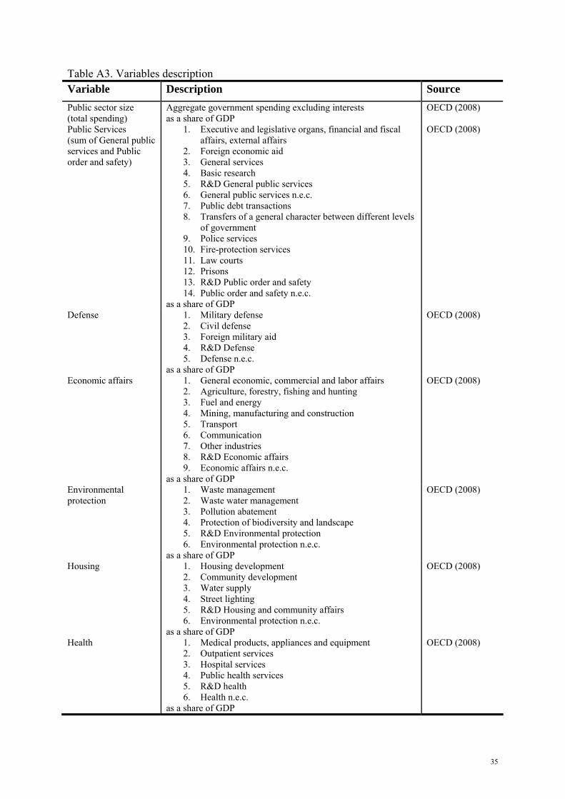
35

Table A3. Variables description Variable Description Source Public sector size (total spending)

Aggregate government spending excluding interests as a share of GDP

OECD (2008)

Public Services (sum of General public services and Public order and safety)

1. Executive and legislative organs, financial and fiscal affairs, external affairs

2. Foreign economic aid 3. General services 4. Basic research 5. R&D General public services 6. General public services n.e.c. 7. Public debt transactions 8. Transfers of a general character between different levels

of government 9. Police services 10. Fire-protection services 11. Law courts 12. Prisons 13. R&D Public order and safety 14. Public order and safety n.e.c.

as a share of GDP

OECD (2008)

Defense 1. Military defense 2. Civil defense 3. Foreign military aid 4. R&D Defense 5. Defense n.e.c.

as a share of GDP

OECD (2008)

Economic affairs 1. General economic, commercial and labor affairs 2. Agriculture, forestry, fishing and hunting 3. Fuel and energy 4. Mining, manufacturing and construction 5. Transport 6. Communication 7. Other industries 8. R&D Economic affairs 9. Economic affairs n.e.c.

as a share of GDP

OECD (2008)

Environmental protection

1. Waste management 2. Waste water management 3. Pollution abatement 4. Protection of biodiversity and landscape 5. R&D Environmental protection 6. Environmental protection n.e.c.

as a share of GDP

OECD (2008)

Housing 1. Housing development 2. Community development 3. Water supply 4. Street lighting 5. R&D Housing and community affairs 6. Environmental protection n.e.c.

as a share of GDP

OECD (2008)

Health 1. Medical products, appliances and equipment 2. Outpatient services 3. Hospital services 4. Public health services 5. R&D health 6. Health n.e.c.

as a share of GDP

OECD (2008)

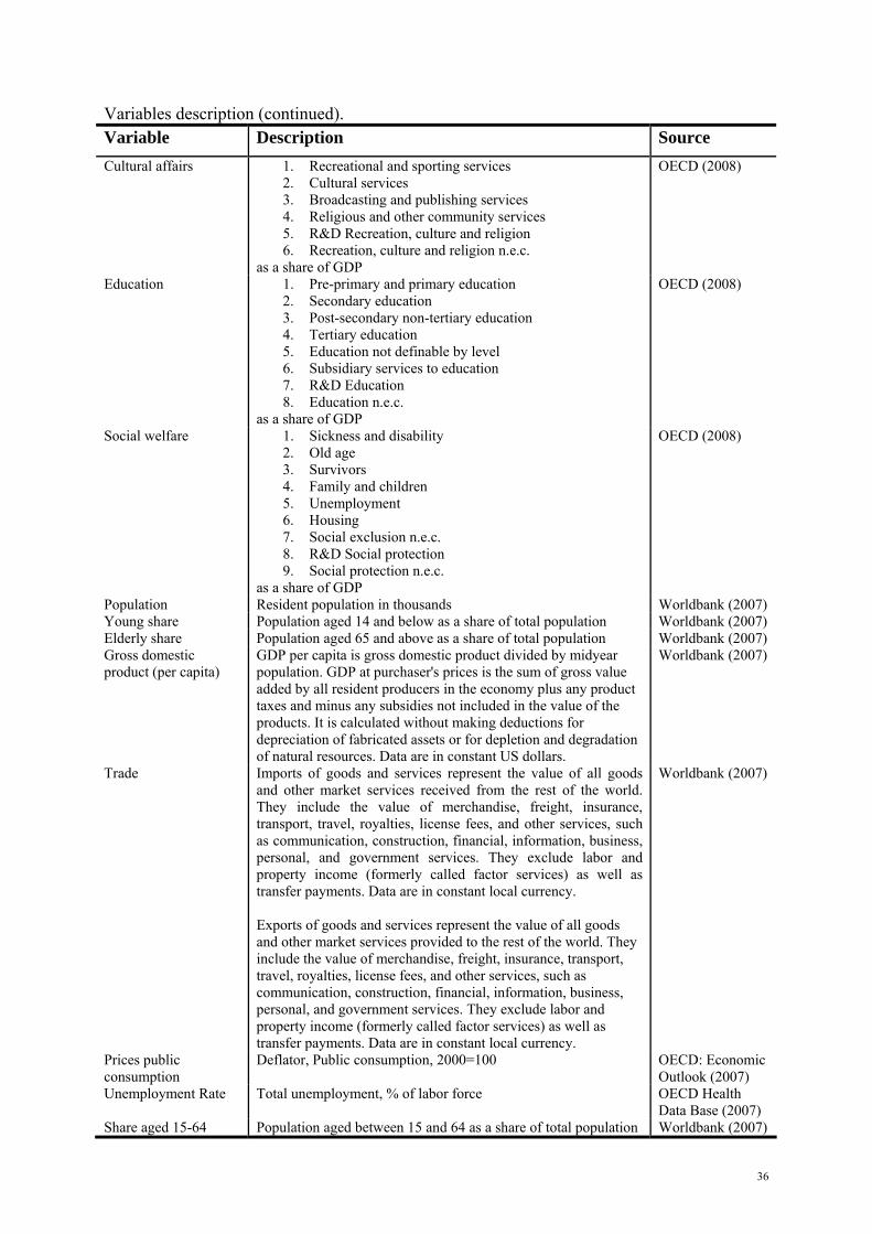
36

Variables description (continued). Variable Description Source Cultural affairs 1. Recreational and sporting services

2. Cultural services 3. Broadcasting and publishing services 4. Religious and other community services 5. R&D Recreation, culture and religion 6. Recreation, culture and religion n.e.c.

as a share of GDP

OECD (2008)

Education 1. Pre-primary and primary education 2. Secondary education 3. Post-secondary non-tertiary education 4. Tertiary education 5. Education not definable by level 6. Subsidiary services to education 7. R&D Education 8. Education n.e.c.

as a share of GDP

OECD (2008)

Social welfare 1. Sickness and disability 2. Old age 3. Survivors 4. Family and children 5. Unemployment 6. Housing 7. Social exclusion n.e.c. 8. R&D Social protection 9. Social protection n.e.c.

as a share of GDP

OECD (2008)

Population Resident population in thousands Worldbank (2007) Young share Population aged 14 and below as a share of total population Worldbank (2007) Elderly share Population aged 65 and above as a share of total population Worldbank (2007) Gross domestic product (per capita)

GDP per capita is gross domestic product divided by midyear population. GDP at purchaser's prices is the sum of gross value added by all resident producers in the economy plus any product taxes and minus any subsidies not included in the value of the products. It is calculated without making deductions for depreciation of fabricated assets or for depletion and degradation of natural resources. Data are in constant US dollars.

Worldbank (2007)

Trade Imports of goods and services represent the value of all goods and other market services received from the rest of the world. They include the value of merchandise, freight, insurance, transport, travel, royalties, license fees, and other services, such as communication, construction, financial, information, business, personal, and government services. They exclude labor and property income (formerly called factor services) as well as transfer payments. Data are in constant local currency. Exports of goods and services represent the value of all goods and other market services provided to the rest of the world. They include the value of merchandise, freight, insurance, transport, travel, royalties, license fees, and other services, such as communication, construction, financial, information, business, personal, and government services. They exclude labor and property income (formerly called factor services) as well as transfer payments. Data are in constant local currency.

Worldbank (2007)

Prices public consumption

Deflator, Public consumption, 2000=100 OECD: Economic Outlook (2007)

Unemployment Rate Total unemployment, % of labor force OECD Health Data Base (2007)

Share aged 15-64 Population aged between 15 and 64 as a share of total population Worldbank (2007)

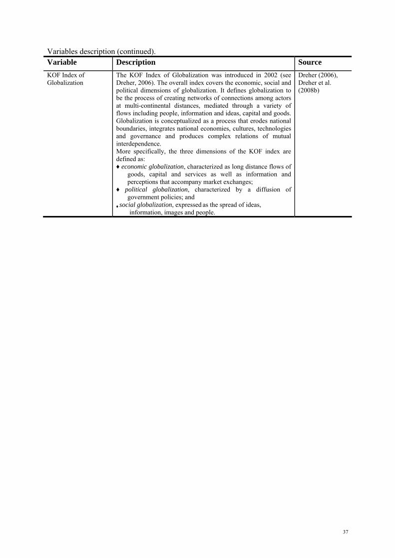
37

Variables description (continued). Variable Description Source KOF Index of Globalization

The KOF Index of Globalization was introduced in 2002 (see Dreher, 2006). The overall index covers the economic, social and political dimensions of globalization. It defines globalization to be the process of creating networks of connections among actors at multi-continental distances, mediated through a variety of flows including people, information and ideas, capital and goods. Globalization is conceptualized as a process that erodes national boundaries, integrates national economies, cultures, technologies and governance and produces complex relations of mutual interdependence. More specifically, the three dimensions of the KOF index are defined as: ♦ economic globalization, characterized as long distance flows of

goods, capital and services as well as information and perceptions that accompany market exchanges;

♦ political globalization, characterized by a diffusion of government policies; and

♦ social globalization, expressed as the spread of ideas, information, images and people.

Dreher (2006), Dreher et al. (2008b)