Does government size affect per-capita income growth?

A Hierarchical meta-regression analysis

Sefa Awawoyi Monash University

Mehmet Ugur University of Greenwich

And

Siew Ling Yew Monash University

Year: 2015

No: GPERC20

2

Abstract: We conduct a hierarchical meta-regression analysis to review 87 empirical studies that report

769 estimates for the effects of government size on economic growth. We follow best-practice

recommendations for meta-analysis of economics research, and address issues of publication selection bias

and heterogeneity. When size is measured as the ratio of total government expenditures to GDP, the partial

correlation between government size and per-capita GDP growth is negative in developed countries, but

insignificant in developing countries. When size is measured as the ratio of consumption expenditures to

GDP, the partial correlation is negative in both developed and developing countries, but the effect in

developing countries is less adverse. We also report that government size is associated with less adverse

effects when primary studies control for endogeneity and are published in journals and more recently, but

it is associated with more adverse effects when primary studies use cross-section data. Our findings indicate

that the relationship between government size and per-capita GDP growth is context-specific and likely to

be biased due to endogeneity between the level of per-capita income and government expenditures.

JEL code: O40, H50, C1

Keywords: Economic growth; Government size; Government expenditure; Government consumption;

Meta-analysis; Evidence synthesis

Acknowledgements: We would like to thank two anonymous reviewers of the Program Committee of

MAER-Net Colloquium 2015 in Prague; and the participants in the conference for helpful comments.

Correspondinf Author: Sefa Awawoyi Churchill: Department of Economics, Monash University, VIC

3800, Australia. Email: sefa.awaworyi@monash.edu

Siew Ling Yew: Department of Economics, Monash University, VIC 3800, Australia. Email:

siew.ling.yew@monash.edu

Mehmet Ugur: Business School, University of Greenwich, London, UK. Email: m.ugur@gre.ac.uk

3

1. Introduction

One of the most contentious issues in economics is whether ‘big government’ is good or bad for

economic growth. From the mid-1980s onwards, the received wisdom has been that big

government is detrimental to growth. This consensus has been tested by the onset of the recent

financial crisis in Europe and the United States (US), which has called on governments to act not

only as lenders of last resort but also as demand-managing and bank-nationalising fiscal

heavyweights, the spending capacity of which was a crucial ingredient for recovery. Yet, it would

be premature to claim that the consensus has lost its appeal. The financial crisis has also meant

that a large number of European countries (including not only fiscally-vulnerable Greece, Ireland,

Italy, Portugal and Spain, but also fiscally-comfortable countries such as Germany and the UK)

had to embark on austerity programs with the aim of not only reducing budget deficits but also

creating room for private investment as an engine of growth.

The continued appeal of the received wisdom may be due to ambiguity in the economic

theory. Theoretically, big government can have both negative and positive effects on growth. On

the one hand, big government can affect growth adversely because of crowding-out effects on

private investment (Landau, 1983; Engen and Skinner, 1992). Big government also implies high

taxes, most of which are growth-reducing due to their distortionary nature (De Gregorio, 1992).

Increased government size can also be a source of inefficiency due to rent seeking and political

corruption that harm economic growth (Hamilton, 2013; Gould and Amaro-Reyes, 1983; Mauro,

1995).

On the other hand, however, government can play a growth-enhancing role by providing

public goods, minimising externalities, ensuring rule of law, and maintaining confidence in a

4

reliable medium of exchange. Government also can contribute to growth by enhancing human

capital through investments in health and education and by building and maintaining a sound

infrastructure (Kormendi and Meguire, 1985; Ram, 1986; De Witte and Moesen, 2010). From a

Keynesian perspective increased government spending increases aggregate demand that in turn

induces an increase in aggregate supply.

The empirical literature on the issue is also inconclusive. On the one hand, a large number

of studies report a negative relationship between government size and growth (see, e.g., Grier and

Tullock, 1989; Barro, 1991; Lee, 1995; Ghura, 1995; Fölster and Henrekson, 2001; among others).

On the other hand, a sizeable number report a positive relationship (see, e.g., Aschauer, 1989;

Munnell, 1990; Evans and Karras, 1994).

Such heterogeneous findings are not surprising not only because of the ambiguity of the

theoretical predictions but also because government size is usually measured differently,1 countries

may be at different stages of development, and they may have different political/institutional

structures that affect the optimal government size (Bergh and Karlsson, 2010). In addition, model

specification as well as estimation methods differ between studies. Beyond such sources of

heterogeneity, findings from earlier studies have indicated that the effect of government size on

growth is either not robust to model specification (Levine and Renelt, 1992) or does not remain a

significant determinant of growth in a series of Bayesian averaging trials (Sala-i-Martin et al.,

2004).2

1Government consumption tends to capture public outlays that are not productivity enhancing. It is often measured as all

government expenditures for goods and services but excluding government military expenditure, and in some cases education

expenditures (see, e.g., Barro, 1991; Easterly and Rebelo, 1993). According to the OECD, total government expenditure, on the

other hand, captures the total amount of expenditure by government that needs to be financed via government revenues. 2 In contrast, Sala-i-Martin et al. (2004) report that government consumption has a negative effect on growth (-0.034). Surprisingly,

however, the adverse effect of government consumption is less severe than that of public investment (-0.062).

5

Given this landscape, there is evident need to synthesize the existing evidence on the relationship

between government size and growth. The synthesis should address not only the question of

whether government size is growth-enhancing or growth-retarding, but also the sources of

heterogeneity in the evidence base, and whether or not the reported evidence is robust to

endogeneity and reverse causality, data type and model specification.

A number of past reviews have already tried to synthesize the existing findings (see, e.g.,

Poot, 2000; Nijkamp and Poot, 2004; and Bergh and Henrekson, 2011). Some of these reviews

focus on the growth-effects of specific types of government expenditures; but others (e.g. Bergh

and Henrekson, 2011) focus explicitly on government size and growth. These reviews provide

useful narrative syntheses that reflect the state of the art in the research field, but they are not suited

to make inferences about either the ‘effect size’ or the effects of the moderating factors on the

heterogeneity in the evidence base for three reasons. First, they do not take account of all effect-

size estimates reported by the primary studies. Secondly, their selection of the primary studies is

not systematic and as such their findings may be subject to sample selection bias. Last but not

least, they do not address the risk of publication selection bias that arises when authors or editors

are predisposed to publish significant findings or findings that support a given hypothesis.

Thus, this study aims to contribute to the existing literature in three areas. First, we address the

issue of publication bias and establish whether government size has a ‘genuine’ growth effect

beyond publication bias. Second, we examine the potential sources of heterogeneity in the

evidence base and demonstrate how these moderating factors influence the reported effect-size

estimates. Third, we synthesize the evidence with respect to: (a) two measures of government size

(total government expenditures and government consumption); and (b) both developed and less

developed countries (LDCs).

6

2. Theoretical and Empirical Considerations

Several perspectives exist on what explains growth.3 The neoclassical growth model (Solow, 1956;

Swan, 1956) has a successful track record in estimating capital and labour elasticities (i.e., capital

and output shares in output) at the macro, industry and firm levels. However, the model has a

number of shortcomings.4 From the perspective of this review, the most important implication of

the Solow-type growth model is that it has to be augmented with a measure of government size

even though the latter is not theorised to have any effect on long-run growth rates.

In endogenous growth models, cross-country differences in per-capita income can persist

indefinitely. These models have the advantage of taking into account the out-of-steady-state

dynamics and the factors that affect the level of technology (Romer, 1986; Barro, 1990). In these

models, government policy can alter the level of endogenous variables such as human capital or

investment rates; and may have theory-driven implications for the country’s long-run growth.

Hence, one factor that is likely to cause heterogeneity in the empirical evidence is the theoretical

model utilised in the empirical studies. Some studies augment the neo-classical growth model with

government size (𝐺), which yields a generic model of the type below:

𝑌𝑖𝑡 = 𝐴𝑒𝜆𝑡𝐾𝑖𝑡𝛼𝐿𝑖𝑡

𝛽𝐺𝑖𝑡

𝛾𝑒𝑢𝑖𝑡 (1)

3 See Poot (2000) and Bergh and Henrekson (2011) for a detailed overview on the theoretical arguments and models on the

determinants of growth. 4 First, the model is about steady-state level of income. Deviation of a country from its steady-state is temporary or random.

Secondly, the main source of growth (i.e., technology) is exogenous, not observed in the model and the resulting total factor

productivity (TFP) can be captured only through the residuals of the estimated model. Finally, the model predicts unconditional

cross-country convergence of the per-capita income levels – a prediction that runs counter to evidence indicating persistent

divergence in cross-country per-capita income levels.

7

Dividing the inputs and the output by labour (𝐿), allowing for flexible returns to scale, taking

natural logarithms and denoting 𝑙𝑜𝑔(𝐴) with 𝜂𝑖, we obtain:

𝑦𝑖𝑡 = 𝜂𝑖 + 𝜆𝑡 + 𝛼𝑘𝑖𝑡 + 𝛽𝑙𝑖𝑡 + 𝛾𝑔𝑖𝑡 + 𝑢𝑖𝑡 (in levels) (1a)

∆𝑦𝑖𝑡 = ∆𝜆𝑡 + 𝛼∆𝑘𝑖𝑡 + 𝛽∆𝑙𝑖𝑡 + 𝛾∆𝑔𝑖𝑡 + 𝑣𝑖𝑡 (in terms of growth rates) (1b)

Specifications that include 𝑔𝑖𝑡 instead of ∆𝑔𝑖𝑡 as a regressor are widely used for assessing the

impact of government size on economic growth, as the studies by Rubinson (1977) and Landau

(1983) indicate, thus the estimated growth model may take the form:

∆𝑦𝑖𝑡 = ∆𝜆𝑡 + 𝛼∆𝑘𝑖𝑡 + 𝛽∆𝑙𝑖𝑡 + 𝛾𝑔𝑖𝑡 + 𝜀𝑖𝑡 (1c)

In (1a), subscripts 𝑖 and 𝑡 represent country and time, respectively. 𝑌 is income level, which is a

function of capital stock (𝐾) and labour force (𝐿). Augmenting (1) with government size (𝐺) has

been proposed by Feder (1983) and Ram (1986); and 𝐺 can be measured as government

expenditures or government consumption.5 The small-case letters (𝑘, 𝑙, 𝑔) are the logarithms of

capital per-capita, labour and government size. Finally, 𝜂𝑖 is country fixed effect, 𝜆𝑡 is time trend

and 𝑢𝑖𝑡 is an idiosyncratic error term.

Empirical studies included in this review, such as Grossman (1990), Atesoglu and Mueller

(1990) and Dar and AmirKhalkhali (2002) among others, utilize version (1c) of the growth model.

The parameter of interest, 𝛾, is the effect of government size on per-capita income growth. All

other variables are as defined in 1(a).

5 In (1a), constant returns to scale are not imposed. Hence the coefficient on labour (l) indicates increasing, decreasing or constant

returns to scale – depending on whether 𝛽 is greater than, smaller than or equal to zero.

8

Government size (𝐺) is measured as total expenditures or consumption expenditures as a

ratio of income (usually, gross domestic product – GDP). Some studies use the ratio of government

size to GDP in level (𝐺), some others use the logarithm of the ratio (𝑔) providing an elasticity

estimate of the effect size. In the former, the effect size (𝛾) is not comparable across studies if the

metrics with which 𝐺 and 𝑌 are measured are different; in the latter, the effect size (𝛾) is

comparable across studies irrespective of the metrics with which 𝐺 and 𝑌 are measured.

A considerable number of studies also adopt a variant of the endogenous growth model.

These studies follow Barro (1991) and Mankiw et al. (1992), where the determinants of growth

include investment in physical capital (𝐾) and human capital (𝐻), augmented with other covariates

such as government expenditures (𝐺) and other variables found to be related to growth in the

empirical literature (e.g., initial level of per-capita GDP, openness, financial development, etc.).

The endogenous models usually take the following form:

∆𝑦𝑖𝑡 = 𝛼𝐾𝑖𝑡 + 𝛽𝐻𝑖𝑡 + 𝛾𝐺𝑖𝑡 + ∑ 𝜃𝑗𝑍𝑗,𝑖𝑡

𝑗

+ 𝜀𝑖𝑡 (2)

Here, ∆𝑦𝑖𝑡is the growth rate of per-capita GDP and 𝐺 is the share of government expenditure to

GDP. 𝑍𝑗 is a vector of variables commonly used in the economic growth literature, including

financial deepening or institutional quality, etc. Subscripts 𝑖 and 𝑡 represent country and time,

respectively. This specification has been widely used in the empirical growth literature, including

Barro and Sala-i-Martin (1995), Stroup and Heckelman (2001) and Bose et al. (2007).

There are also hybrid models - including simultaneous equation models where government size is

modelled to have both direct and indirect effects on growth and Keynesian models where

government size affects growth from both the demand and supply side (see, e.g., Tanninen, 1999;

9

Ghosh and Gregoriou, 2008). We include studies using hybrid models, but we consider only their

estimates of the direct effect.

We meta-analyse the effect-size estimates only if they are reported by studies that utilize:

(a) the ratio of government expenditures or consumption to GDP as the independent variable; and

(b) the growth rate of per-capita GDP as the outcome variable.

To account for heterogeneity due to model choice, we control for endogenous growth

models and treat the exogenous model as the reference category. Furthermore, both neoclassical

and endogenous growth models (1c and 2) are used with panel and/or cross-section data averaged

over a long period. Furthermore, panel-data studies may report estimates based on annual data or

on data averaged over some years to smooth out the business cycle. These variations are additional

sources of heterogeneity in the evidence base. To account for this, we code each estimate not only

with respect to the growth model it is derived from but also with respect to data type and the

number of years over which the panel data is averaged.

Other sources of heterogeneity include: (i) whether primary studies control for endogeneity

through instrumental variable or dynamic panel-data techniques; (ii) the range of control variables

included in estimated models; (iii) publication type (e.g., journal articles, working papers, book

chapters, reports, etc.); (iv) publication date; (v) journal quality ranking; (vi) country type

(developed versus less developed); (vii) length of periods over which data is averaged in cross-

section and panel-data studies; and (viii) the data period. We code the effect-size estimates

accordingly and control for these sources of heterogeneity within a multiple meta-regression

setting.

10

3. Data and an overview of the evidence base

Our meta-analysis methodology draws on guidelines proposed by the Meta-analysis of Economics

Research Network (MAER-Net), which reflects best practices and transparency in meta-analyses

(Stanley et al., 2013). We searched five electronic databases - JSTOR, EconLit, Business Source

Complete, Google Scholar and ProQuest - for journal articles, working papers and book chapters;

using various keywords for government size and growth.6 We also conduct a manual search where

we examine the references of key reviews and studies that examine the government size-growth

relationship to ensure that other relevant studies are included in our meta-analysis.

In this study, we include all effect-size estimates reported by empirical studies that examine

the direct effect of government size on growth. The independent variable must be either total

government expenditure or government consumption expenditure, and must be measured as a

proportion or share of GDP. The dependent variable must be the growth rate of per capita GDP.

Thus, we exclude studies that use other measures of government size such as expenditure or

consumption levels or the growth rate of government expenditures/consumption. We also exclude

studies that estimate the effects of government size on GDP levels instead of per-capita GDP

growth.

Adhering to the above inclusion/exclusion criteria, our meta-analysis consists of 87 primary

studies reporting 769 estimates on the relationship between government size and growth. Table

1A presents an overview of the studies that report on the effect of total government expenditure,

6 The keywords for government size include total government expenditures, government consumption, government spending,

outlays, public spending, public expenditures, and public consumption. Keywords for economic growth include GDP, per capita

income, growth, economic performance, and economic activity.

11

while Table 1B presents the overview of those reporting on the effect of government consumption

only.

4. Meta-analysis tools and findings

The meta-analysis methods adopted in this study have been used previously in various studies (see,

e.g., Abreu et al., 2005; Alptekin and Levine, 2012; Stanley and Doucouliagos, 2012 and Ugur,

2014). Therefore, we elaborate on the methods and tools in the Appendix and present the results

in the main text to achieve brevity and continuous flow.

4.1. Partial correlation coefficients (PCCs) and fixed effect weighted means (FEWMs)

Given the variety of the metrics with which the dependent and outcome variables are measured,

we calculate PCCs for each effect-size estimate to allow for comparability between and within

primary studies (see Appendix). We also calculate FEWMs of the PCCs for each primary study

and for two samples consisting of studies that investigate the growth effects of total government

expenditures (Table 1A) and government consumption (Table 1B). As summary measures,

FEWMs are considered more reliable than simple means, and also less affected by publication bias

compared to random effects weighted averages (Stanley, 2008; Henmi and Copas, 2010; Stanley

and Doucouliagos, 2014).

[Tables 1A and 1B]

12

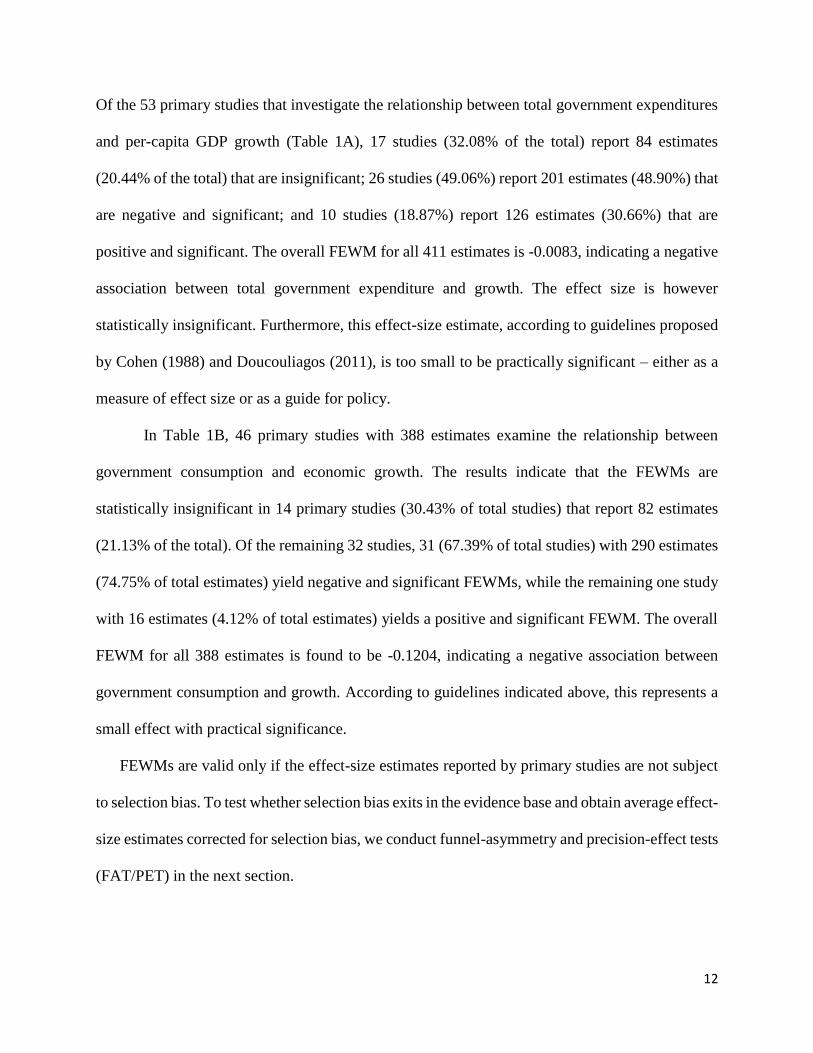
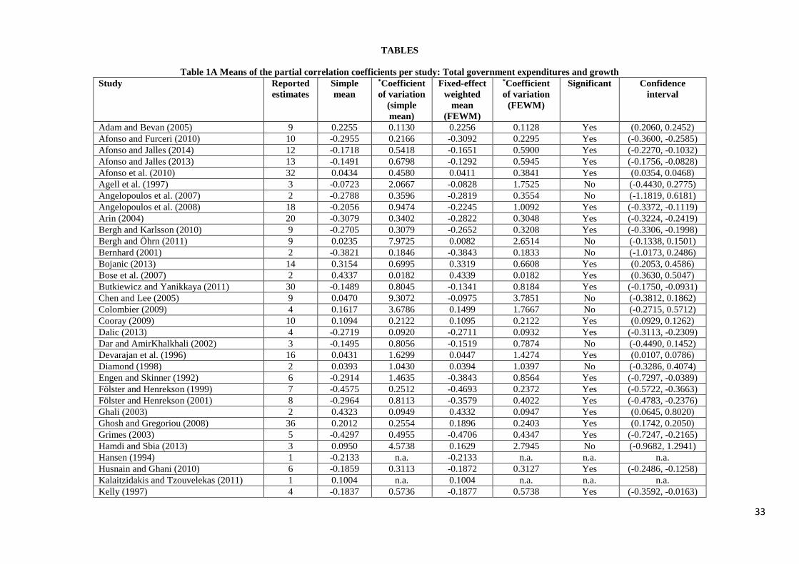
Of the 53 primary studies that investigate the relationship between total government expenditures

and per-capita GDP growth (Table 1A), 17 studies (32.08% of the total) report 84 estimates

(20.44% of the total) that are insignificant; 26 studies (49.06%) report 201 estimates (48.90%) that

are negative and significant; and 10 studies (18.87%) report 126 estimates (30.66%) that are

positive and significant. The overall FEWM for all 411 estimates is -0.0083, indicating a negative

association between total government expenditure and growth. The effect size is however

statistically insignificant. Furthermore, this effect-size estimate, according to guidelines proposed

by Cohen (1988) and Doucouliagos (2011), is too small to be practically significant – either as a

measure of effect size or as a guide for policy.

In Table 1B, 46 primary studies with 388 estimates examine the relationship between

government consumption and economic growth. The results indicate that the FEWMs are

statistically insignificant in 14 primary studies (30.43% of total studies) that report 82 estimates

(21.13% of the total). Of the remaining 32 studies, 31 (67.39% of total studies) with 290 estimates

(74.75% of total estimates) yield negative and significant FEWMs, while the remaining one study

with 16 estimates (4.12% of total estimates) yields a positive and significant FEWM. The overall

FEWM for all 388 estimates is found to be -0.1204, indicating a negative association between

government consumption and growth. According to guidelines indicated above, this represents a

small effect with practical significance.

FEWMs are valid only if the effect-size estimates reported by primary studies are not subject

to selection bias. To test whether selection bias exits in the evidence base and obtain average effect-

size estimates corrected for selection bias, we conduct funnel-asymmetry and precision-effect tests

(FAT/PET) in the next section.

13

4.2. Effect size beyond publication selection

The precision-effect test (PET) and the funnel-asymmetry test (FAT) involve the estimation of a

weighted least square bivariate model, in which the effect-size estimate is a function of its standard

error (see Egger et al., 1997; Stanley, 2008). Furthermore, Stanley and Doucouliagos (2007)

propose that precision-effect estimation with standard errors (PEESE) can be used to obtain an

estimate corrected for non-linear relationship between effect size and its standard error (see

Appendix). The PEESE should be conducted only if PET/FAT procedure indicates the existence

of a genuine effect beyond publication selection bias.

We estimate PET-FAT-PEESE models for two measures of government size: total

government expenditures and government consumption expenditures; and for developed and

LDCs. Our estimates are obtained using a hierarchical linear model (HLM) specification

(Goldstein, 1995), whereby individual effect-size estimates are nested within studies reporting

them. The choice of HLM is informed by the data structure at hand. The effect-size estimates are

nested within each study where data, model specification and estimation method are significant

sources of dependence between reported estimates. The appropriateness of the HLM is verified

through a likelihood ratio (LR) test that compares the HLM with standard OLS; whereas the type

of HLM is determined by LR tests that compare random effects intercepts with random effects

intercepts and slopes.7 The PET-FAT-PEESE results are presented in Tables 2A and 2B, for two

full samples and for two country types (developed and LDCs) within each sample.

7 The HLM is employed to deal with data dependence by De Dominicis et al. (2008), Bateman and Jones (2003), and Alptekin and

Levine (2012), among others. The likelihood ratio test results that compare HLM with OLS and the types of HLM structures are

available on request.

14

[Tables 2A and 2B]

Regarding total government expenditure and growth, we find no evidence of genuine effect in the

full sample or in LDCs as the coefficient of the precision is statistically insignificant (columns 1

and 3 of Table 2A). In the developed countries sample (column 2 of Table 2A), we find evidence

of a negative effect (-0.13) without evidence of publication selection bias. This PET-FAT result is

also supported by the PEESE result (Column 4) with a slightly more adverse effect (-0.14). Thus,

with respect to total government expenditure as a proxy for government size, we report a negative

partial correlation with growth in developed countries only.

With regard to government consumption and growth (Table 2B), we find evidence of a

negative effect together with significant negative publication selection bias for the entire sample

(column 1) and for the developed countries sample (column 2), but no significant effect for the

LDC sample (column 3). PEESE results that correct for non-linear relations between effect-size

estimates and their standard errors (columns 4 and 5) confirm the existence of negative effects for

the full sample and for developed-country sample (-0.10 and -0.14, respectively).

Statistical significance in the empirical literature has been clearly distinguished from

economic (or practical) significance, especially when the size of a statistically significant

coefficient is small (Ziliak and McCloskey, 2004). Cohen (1988) indicates that an estimate

represents a small effect if its absolute value is around 0.10, a medium effect if it is 0.25 and over,

and a large effect if it is greater than 0.4. Doucouliagos (2011) argues that the guidelines presented

by Cohen (1988) understate the economic significance of empirical effect when partial correlation

coefficients (PCCs) are used. Thus, Doucouliagos (2011) suggests that PCCs larger than the

absolute value of 0.33 can be considered as indicators of ‘large’ effect, while those above (below)

0.07 can be considered ‘medium’ (‘small’).

15

In the light of the guidance proposed by Doucouliagos (2011), these findings indicate that: (i) total

government expenditures have a medium and adverse effect on per-capita income growth in

developed countries only; (ii) the effect of government consumption on per-capita income growth

is also medium in developed countries and in developed and LDCs pooled together; and (iii)

neither total expenditures nor government consumption has a significant effect on per-capita

income growth in LDCs.

However, both FEWMs and PEESE results have limited applicability because they conceal

a high degree of variation in the evidence base. Indeed, the coefficient of variation for full-sample

PCCs in Table 1A and 1B are 9.11 and 1.28, respectively. In addition, the FEWMs and PEESE

results are based on the assumption that, apart from the standard errors, all other moderating factors

that affect the reported estimates are either zero (in the case of FEWMs) or at their sample means

(in the case of PEESE). This assumption is too restrictive because the moderating factors that

influence the effect-size estimates reported in primary studies differ between studies and between

estimates reported by the same study. Therefore, it is necessary to identify the moderating factors

(i.e., the sources of variation) in the evidence base and quantify their influence on the effect-size

estimates reported in primary studies. This is done in the next section, followed by a detailed

discussion of the implications for the government size – growth relationship in the conclusions

and discussion section.

4.3. Addressing Heterogeneity

To identify the sources of heterogeneity and quantify their influence on the reported effect-size

estimates, we estimate a multivariate meta-regression model (MRM) for each sample (i.e., for total

16

government expenditures and government consumption). As indicated in the appendix, we

estimate a general and a specific MRM for each sample. The general specification includes all

moderating factors that can be measured on the basis of the information we obtain from the primary

studies. However, the inclusion of all observable moderating factors poses issues of over-

determination and multicollinearity. Therefore, we follow a general-to-specific model routine,

which involves the exclusion of the moderating variables with high p-values (highly insignificant

variables) one at a time until all remaining variables are statistically significant.8

Three main dimensions of primary study characteristics are captured by our moderator

variables. These moderator variables are informed by the theoretical, empirical and

methodological dimensions of primary studies, as well as other differences presented by primary

studies that are likely to affect the government size-growth relationship. The first set of moderator

variables capture the variations in econometric specifications and theoretical models adopted by

the primary studies. The second category captures data characteristics in primary studies, and the

third examines the publication characteristics of the primary studies. Summary statistics for

moderator variables and their description are presented in Tables 3A and 3B.

[Tables 3A and 3B]

Results from the general and specific MRMs are presented in Table 4A (for total government

expenditures) and Table 4B (for government consumption) below. The general models include 20

moderating variables that capture the three dimensions of the research field indicated above. The

paragraphs below summarize the findings and interpret their implications for the relationship

between government size and per-capita income growth.

8 See Campos et al. (2005) for a detailed discussion on the general-to-specific modelling literature.

17

Theoretical Models and Econometric Specifications

To investigate if differences in underlying theoretical models affect the government size-growth

relationship, we use a dummy variable that controls for studies that base their specification on

endogenous growth models and exclude studies that use the Solow-type growth model as base.

From Table 4A, we find that the underlying theoretical model does not have a significant effect on

reported effect-size estimates when the latter are about the effects of total government expenditures

on per-capita income growth. However, we note from Table 4B that studies that utilize an

endogenous growth model tend to report more adverse effect-size estimates for the relationship

between government consumption and per-capita income growth.

[Tables 4A and 4B]

With respect to econometric dimension, we first examine the difference between estimates based

on cross-section data as opposed to panel-data or time-series data. This control is relevant because

cross-section estimations overlook fixed effects that may reflect country-specific difference in

preferences and technology. In the presence of fixed-effects, estimates based on cross-section data

may yield biased results. Panel-data estimations can address this source of bias by purging the

country-specific fixed effects and focusing on temporal variations in the data.

In Table 4A where the focus is on total government expenditures, we find that the use of

cross-section data (as opposed to panel data) is associated with more adverse effects on growth,

but the effect is insignificant. However, when government size is proxied by consumption (Table

4B), the use of cross-section data is associated with more adverse effects; and the coefficient is

significant. We also control for studies that use time-series data as opposed to cross-section and

18

panel data. In both total expenditures (Table 4A) and consumption expenditures (Table 4B)

samples, we find no statistically significant effects. Hence, we conclude that the use of cross-

section data is likely to be a source of negative bias in the evidence base. Therefore, it is likely

that the negative association between government consumption and growth referred to in the public

and policy debate should be qualified.

The second dimension of the econometric specification we consider is model specification.

In the empirical growth literature, it is well known that the inclusion (or exclusion) of certain

regressors in growth regressions can affect the reported effect-size estimate. Levine and Renelt

(1992) indicate that initial GDP per capita, investment share of GDP and population are important

growth determinants. Hence, we include dummies for studies that control for these variables. We

also include a dummy for studies that control for tax in their growth regressions, given that the

distortionary effects of taxation feature as a major factor in the debate on government size and

growth.

MRM results in Tables 4A and 4B confirm that the inclusion of these variables in growth

regressions tend to affect the estimates reported in primary studies. For instance, in Table 4A, we

find that studies that control for investment, population or initial GDP (compared to those that do

not) tend to report more adverse effects. Results from Table 4B show that studies that control for

investment (compared to those that do not) tend to report less adverse effects whereas the opposite

is observed for those that control for population.

Therefore, the inclusion or exclusion of key determinants of growth in the regression

significantly alters the magnitude of the reported effect size estimates, but the effect is not

consistent across the measures of government size. Despite the variation, we argue that it would

be good practice for researchers to include the key regressors in their regressions with a view to

19

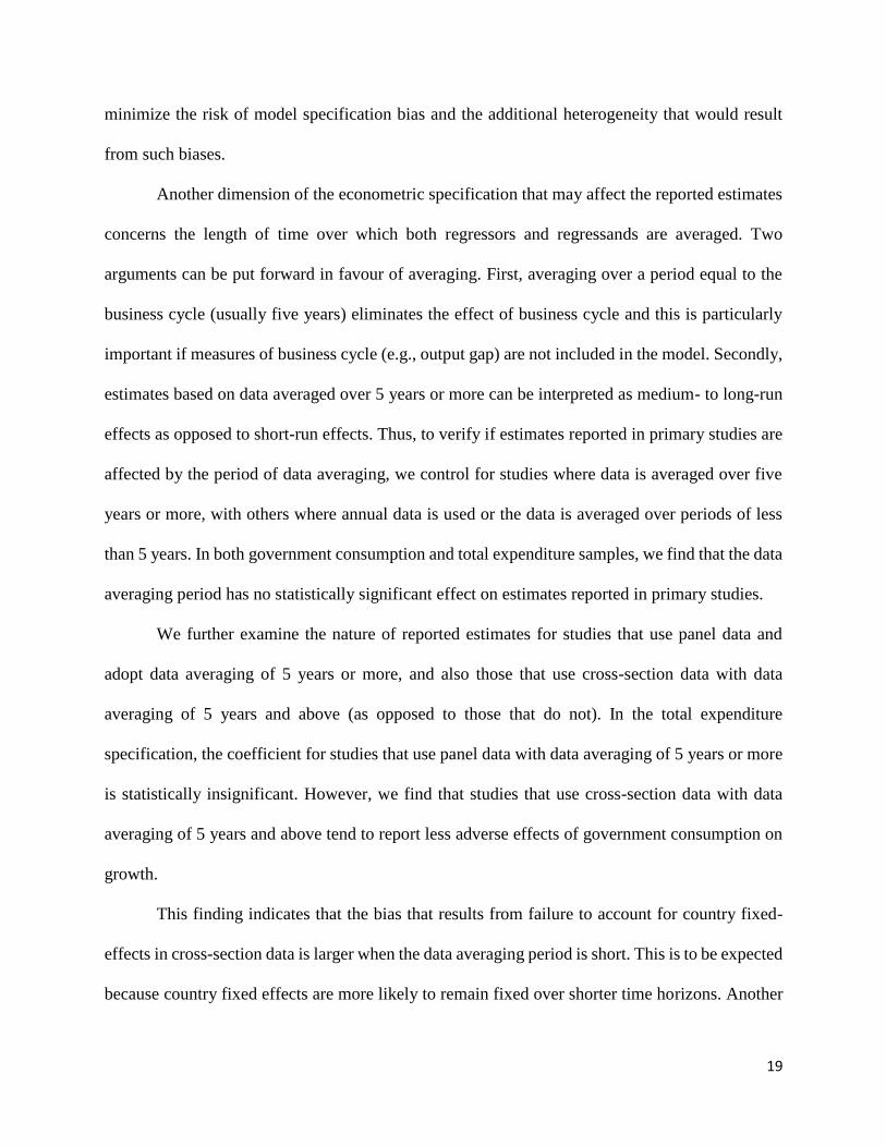
minimize the risk of model specification bias and the additional heterogeneity that would result

from such biases.

Another dimension of the econometric specification that may affect the reported estimates

concerns the length of time over which both regressors and regressands are averaged. Two

arguments can be put forward in favour of averaging. First, averaging over a period equal to the

business cycle (usually five years) eliminates the effect of business cycle and this is particularly

important if measures of business cycle (e.g., output gap) are not included in the model. Secondly,

estimates based on data averaged over 5 years or more can be interpreted as medium- to long-run

effects as opposed to short-run effects. Thus, to verify if estimates reported in primary studies are

affected by the period of data averaging, we control for studies where data is averaged over five

years or more, with others where annual data is used or the data is averaged over periods of less

than 5 years. In both government consumption and total expenditure samples, we find that the data

averaging period has no statistically significant effect on estimates reported in primary studies.

We further examine the nature of reported estimates for studies that use panel data and

adopt data averaging of 5 years or more, and also those that use cross-section data with data

averaging of 5 years and above (as opposed to those that do not). In the total expenditure

specification, the coefficient for studies that use panel data with data averaging of 5 years or more

is statistically insignificant. However, we find that studies that use cross-section data with data

averaging of 5 years and above tend to report less adverse effects of government consumption on

growth.

This finding indicates that the bias that results from failure to account for country fixed-

effects in cross-section data is larger when the data averaging period is short. This is to be expected

because country fixed effects are more likely to remain fixed over shorter time horizons. Another

20

implication of this finding is that the relatively larger adverse effects reported by studies using

cross-section data are likely to be driven by the dominance of the effect-size estimates based on

short time horizons.

The last dimension relating to econometric and theoretical specification concerns the

econometric methodology used by primary studies. In the empirical growth literature, various

econometric methods have been used and these methodologies aim at addressing specific issues.

For instance, OLS estimates have been found to be inconsistent and biased in the presence of

endogeneity. To address endogeneity, some primary studies tend to use instrumental variable (IV)

techniques. Therefore, we control for studies that control for endogeneity as opposed to those that

do not. The coefficient on the dummy for studies that control for endogeneity is found to be

positive and significant in the total expenditure-growth specification but insignificant in the

government consumption-growth specification. This suggests that studies that control for

endogeneity (compared to those that do not) tend to report less adverse effects of total expenditure

on growth.

Data Characteristics

With regards to data characteristics, we first examine if the government size-growth relationship

is time variant. Thus, we include dummy variables to capture the ‘recentness’ of data and how data

time periods affect reported estimates. We include dummy variables to capture the decade in which

the beginning year of the data period falls, and the subsequent years in the data. For instance, a

primary study that uses data from 1983 to 1999 will fall under “Data Period (1980+)”. Put

differently, Data Period (1980+) captures studies where data years equal to or greater than 1980.

Hence, we introduce dummies for data period 1960+, 1970+, 1980+, and 2000+ and exclude the

21

1950+ as base. MRA results for the total expenditure specification mainly show statistically

insignificant coefficients for data period dummies. However, from Table 4B coefficients for data

period dummies are negative and statistically significant. Particularly, we note that the magnitude

of the coefficient increases as the decades increase. Thus, the smallest coefficient is observed for

“Data Period 1960+” and the largest for “Data Period 1990+”. This suggests that studies that use

newer datasets tend to report more adverse effects of government consumption on growth. This is

also the case for total government expenditure as the only included dummy in the general-to-

specific model (Data Period 2000+), is negative and statistically significant as well.

We also examine the effect of country type using a country-type dummy. Although PET-

FAT results reveal a negative effect of big government on growth in developed countries, it is

worthwhile to control for this in our MRA as well. This ensures the inclusion of all relevant

moderator variables that capture the necessary dimensions. We therefore control for studies that

report estimates using data on developed countries as opposed to those that use data from LDCs

and a mixture of both developed and LDCs. Results from Table 4A confirm what the PET-FAT

results suggest. The developed country dummy is significant and negative, suggesting that studies

that use data on developed countries tend to report more adverse effects of total expenditure on

growth compared to those that use LDCs sample and mixed sample. From Table 4B, the coefficient

of studies that use developed countries data is also negative but insignificant.

Publication Characteristics

Under the publication characteristics dimension, we first control for publication type. Here, we

examine if journal articles tend to systematically report different effect sizes in comparison to book

chapters and working papers. This allows us to determine whether researchers, authors and editors

22

are predisposed to publishing and/or accepting studies with statistically significant results that are

consistent with theory to justify model selection. Using book chapters and working papers as base,

we include a dummy for journal articles in our MRA specification. Results reveal that studies

published in journals tend to report less adverse effects of government size on growth. This is

consistent across both measures of government size and specification type (i.e., both general and

general-to-specific).

Furthermore, we examine if the publication outlet used by primary studies presents some

variations in reported estimate. We therefore control for high-ranked journal as opposed to low-

ranked journals.9 From Table 4A, the coefficient for studies published in high-ranked journals is

statistically insignificant. However, studies published in high-ranked journals tend to report more

adverse effects of government consumption on growth (Table 4B).

Next, we control for publication year. Examining publication year enables us to identify

whether more recent studies, as opposed to older studies, tend to report different estimates. Thus,

we include dummy variables similar to those constructed for data period. For instance, studies

published between 1998 and 2013 fall under “Publication Year (1990+)” and those published

between 2001 and 2014 fall under “Publication Year (2000+)”. Leaving 1980+ as base, we control

for studies published in the decades starting 1990, 2000, and 2010. In both government

consumption and total government expenditure specifications, publication year dummies are

significant. Specifically, from Table 4A, we note that dummies for 1990+ and 2000+ are negative

whereas that of 2010+ is positive. Furthermore, the magnitude of the coefficient for studies

published in the 2000s is smaller than those published in the 1990s. Thus, overall, less adverse

9 The Australian Business Dean’s Council (ABDC) and the Australian Research Council (ARC) present classifications for journal

quality. Journals are ranked in descending order of quality as A*, A, B and C. Thus, we introduce a dummy for A* and A ranked

journals (high quality) in our MRA, and use other ranks as base.

23

effects are associated with newer studies that examine the effect of total expenditure on growth.

For the government consumption specification, we observe that dummies for 1990+ and 2000+

are positive while that for 2010+ is negative.

5. Discussion and conclusions

This paper reviews the empirical literature on the association between government size and

economic growth. We focus on total government expenditures and government consumption

expenditures (as a share of GDP) as measures of government size. Results are based on a synthesis

of 87 studies solely examining the effect of the government size measures as specified above on

per-capita GDP growth. We control for publication selection bias and address issues of

heterogeneity in the existing literature.

Drawing on guidelines proposed by Doucouliagos (2011), the PET-FAT-PEESE results

reported above indicate that the average effect of government size on growth, using both proxies

of government size, is medium only in developed countries. The average effect of total government

expenditures is insignificant in LDCs and when both developed and LDCs are pooled together. On

the other hand, the average effect of government consumption is insignificant in LDCs, but it is

medium in developed countries and when both country types are pooled together.

These findings suggest that the existing evidence does not support an overall inference that

establishes a negative relationship between government size and per-capita income growth for

several reasons including: (i) potential biases induced by reverse causality between government

size and per-capita income; (ii) lack of control for country fixed effects in cross-section studies;

24

and (iii) absence of control for non-linear relationships between government size and per-capita

GDP growth.

Furthermore, the effect is specific to the level of development: government size tends to

have a negative effect on per-capita income growth as the level of income increases. This finding

ties in with the Armey curve hypothesis (Armey, 1995), which posits an inverted-U relationship

between government size and economic growth. The theoretical argument here is that government

size may be characterised by decreasing returns. Another theoretical argument relates to the

distortionary nature of taxes, which is minimal for low levels of taxation, but beyond a certain

threshold, they grow rapidly and become extremely large (Agell, 1996). Hence, our findings

suggest that estimates of the relationship between government size and growth obtained from

linear estimations may be biased (see also, Barro, 1990).

In addition, developed countries tend to have well-developed systems of automatic

stabilisers such as social security expenditures and progressive taxation. According to the World

Social Security Report 2010/11, Europe spends between 20 and 30 per cent of GDP on social

security, while in most African countries social security spending accounts only for 4–6 per cent

of GDP.

According to Devarajan et al. (1996), social security expenditures are unproductive and as such

they may be driving the negative relationship between government size and per-capita income

growth in developed countries. However, social security expenditures and other forms of

automatic stabilisers may be conducive to lower growth rates because of the reverse causality they

inject into the government size-growth relationship. As indicated by Bergh and Henrekson (2011),

automatic stabilisers on the expenditure sides would increase as GDP falls. This well-known

feature of the automatic stabilisers introduces a negative bias in the estimates for the effect of

25

government size on growth. The risk of such bias is higher in developed countries with higher

incidence of automatic stabilisers. At a more general level of observation, the risk of reverse

causality is confirmed by our finding that studies that control for endogeneity tend to report less

adverse effects of government size on growth.

Furthermore, the more pronounced negative effects for developed countries may be related

to Wagner’s Law, which indicates that government size increases with the level of income. There

is evidence indicating that the long-run elasticity of government size with respect to growth in

developed countries is large (Lamartina and Zaghini, 2011). In this case, the government size-GDP

ratio for developed countries will grow faster than LDCs for a given increase in GDP. This

additional endogeneity problem leads to what Roodman (2008) describes as ‘the looking glass

problem’. Roodman (1998) demonstrates that the aid-GDP ratio decreases as GDP increases and

this endogeneity leads to strong positive effects of aid on GDP growth. This finding is opposite to

what we observe in this study but proves the point that if government size-GDP ratio is endogenous

to GDP (i.e., if Wagner’s Law holds), then the stronger negative effects reported on developed

countries may be due to either lack of control for endogeneity in the growth regressions or absence

of adequate instruments or both. This conclusion also ties in with our findings from the MRM

(Table 4A) that studies that control for endogeneity report less adverse effects of government size

on growth.

We also find that studies published in journals tend to report less adverse effects compared

to working papers and book chapters. This is consistent across both measures of government size,

and thus raises the question as to whether the negative association between government size and

per-capita income growth may be driven by less rigorous external reviewing processes in the case

of book chapters and working papers. However, we do not wish to overemphasize this because in

26

the government consumption sample, we find that studies published in higher-ranked journals tend

to report more adverse effects of government size on growth. This is an indication of the ‘Winner’s

curse’ - whereby journals with good reputation capitalize on their reputation and publish ‘more

selected’ findings (see Costa-Font et al., 2013; Ugur, 2014).

In conclusion, our findings show that where an evidence base is too diverse, meta-analysis

can be highly effective in synthesizing the evidence base and accounting for the sources of

heterogeneity among reported findings. Our findings in this study indicate that government size is

more likely to be associated with negative effects on per-capita income growth in developed

countries. They also indicate that the medium-sized adverse effects in developed countries may be

biased due to endogeneity and reverse causality problems, which are either unaddressed in a large

segment of the evidence base or the instruments used to address these problems are weak or both.

Therefore, we call for caution in establishing casual links between government size and per-capita

income growth. We also call for use of non-linear models in the estimation of the government size

– growth relationship. As indicated by Agell (1996), non-linear models may provide richer

evidence on the optimal government size, particularly when the latter is measured in terms of tax

revenues. Finally, and as indicated by Kneller et al. (1999), Poot (2000) and Bergh and Henrekson

(2011), we call for further research on the relationship between particular components of the

government size and growth as such studies are more likely to produce policy-relevant findings

compared to studies that focus on total measures of government size.

27

6. References

Abreu, M., de Groot, H., & Florax, R. (2005). A meta-analysis of beta convergence. Tinbergen Institute

Discussion Papers, No. TI 2005-001/3.

Adam, C., & Bevan, D. (2005). Fiscal deficits and growth in developing countries. Journal of Public

Economics 89 (89), 571– 597.

Afonso, A., & Furceri, D. (2010). Government Size, Composition, Volatility and Economic Growth.

European Journal of Political Economy, 26(4), 517-532.

Afonso, A., & Jalles, J. T. (2013). Fiscal composition and long-term growth. Applied Economics, 46(3),

349-358. doi: 10.1080/00036846.2013.848030

Afonso, A., & Jalles, J. T. J. T. (2013). Do Fiscal Rules Matter for Growth? Applied Economics Letters,

20(1-3), 34-40.

Afonso, A. A., Gruner, H. P., Kolerus, C. E., & Grüner, H. P. (2010). Fiscal Policy and Growth: Do

Financial Crises Make a Difference? European Central Bank, Working Paper Series: 1217.

University of Mannheim - Department of Economics ; University of Mannheim - Center for

Doctoral Studies in Economics and Management (CDSEM).

Agell, J. (1996). Why Sweden’s welfare state needed reform. Economic Journal, 106(439), 1760–1771.

Agell, J., Lindh, T., & Ohlsson, H. (1997). Growth and the public sector: A critical review essay. European

Journal of Political Economy, 13(1), 33-52.

Alptekin, A., & Levine, P. (2012). Military expenditure and economic growth: A meta-analysis. European

Journal of Political Economy, 28(4), 636-650.

Andrés, J., Doménech, R., & Molinas, C. (1996). Macroeconomic performance and convergence in OECD

countries. European Economic Review, 40(9), 1683-1704.

Angelopoulos, K., Economides, G., & Kammas, P. (2007). Tax-spending policies and economic growth:

theoretical predictions and evidence from the OECD. European Journal of Political Economy,

23(4), 885-902.

Angelopoulos, K., & Philippopoulos, A. (2007). The Growth Effects of Fiscal Policy in Greece 1960-2000.

Public Choice, 131(1-2), 157-175.

Angelopoulos, K., Philippopoulos, A., & Tsionas, E. (2008). Does Public Sector Efficiency Matter?

Revisiting the Relation between Fiscal Size and Economic Growth in a World Sample. Public

Choice, 137(1-2), 245-278.

Arin, K. P. (2004). Fiscal Policy, Private Investment and Economic Growth: Evidence from G-7 Countries.

Massey University - Department of Commerce.

Armey, D. (1995). The Freedom Revolution. Washington: Regnery Publishing.

Aschauer, D. (1989). Is government spending productive? Journal of Monetary Economics, 23, 177-200.

Atesoglu, H. S., & Mueller, M. J. (1990). Defence spending and economic growth. Defence Economics, 2,

19 - 27.

Barro, R. (1990). Government spending in a simple model of endogenous growth. Journal of Political

Economy, 98(5), S103-S125.

Barro, R. J. (1989). A Cross-Country Study of Growth, Saving, and Government. NBER Working Paper

No. 2855.

Barro, R. J. (1991). Economic Growth in a Cross Section of Countries. The Quarterly Journal of

Economics, 106(2), 407-443.

Barro, R. J. (1996). Determinants of Economic Growth: A Cross-Country Empirical Study. NBER Working

Paper No. 5698.

Barro, R. J. (2001). Human Capital and Growth. American Economic Review, 91(2), 12-17.

Barro, R. J., & Sala-i-Martin, X. (1995). Economic Growth Cambridge, MA: MIT Press.

Bateman, I., & Jones, A. (2003). Contrasting conventional with multi-level modelling approaches to meta-

analysis: expectation consistency in U.K. woodland recreation values. . Land Economics 79(2),

235–258.

28

Bellettini, G., & Ceroni, C. B. (2000). Social Security Expenditure and Economic Growth: An Empirical

Assessment. Research in Economics, 54(3), 249-275.

Benos, N., & Zotou, S. (2014). Education and Economic Growth: A Meta-Regression Analysis. World

Development, 64(0), 669-689.

Bergh, A., & Henrekson, M. (2011). Government Size and Growth: A Survey and Interpretation of the

Evidence. Journal of Economic Surveys, 25(5), 872-897.

Bergh, A., & Karlsson, M. (2010). Government size and growth: Accounting for economic freedom and

globalization. Public Choice, 142(1-2), 195-213.

Bergh, A., & Öhrn, N. (2011). Growth Effects of Fiscal Policies: A Critical Appraisal of Colombier’s

(2009) Study. IFN Working Paper No. 865.

Bernhard, H. (2001). The Scope of Government and its Impact on Economic Growth in OECD Countries.

Kieler Arbeitspapiere, No. 1034.

Bojanic, A. N. (2013). The Composition of Government Expenditures and Economic Growth in Bolivia.

Latin American Journal of Economics, 50(1), 83-105.

Bose, N., Haque, M. E., & Osborn, D. R. (2007). Public Expenditure and Economic Growth: A

Disaggregated Analysis for Developing Countries. Manchester School, 75(5), 533-556.

Brumm, H. J. (1997). Military Spending, Government Disarray, and Economic Growth: A Cross-Country

Empirical Analysis. Journal of Macroeconomics, 19(4), 827-838.

Butkiewicz, J. L., & Yanikkaya, H. (2011). Institutions and the Impact of Government Spending on Growth.

Journal of Applied Economics, 14(2), 319-341.

Campos, J., Ericsson, N., & Hendry, D. (2005). General-to-specific modeling: an overview and selected

bibliography. . FRB International Finance Discussion Paper, (838).

Castro, V. (2011). The Impact of the European Union Fiscal Rules on Economic Growth. Journal of

Macroeconomics, 33(2), 313-326.

Chen, S.-T., & Lee, C.-C. (2005). Government size and economic growth in Taiwan: A threshold regression

approach. Journal of Policy Modeling, 27(9), 1051-1066.

Cohen, J. (1988). Statistical Power Analysis for the Behavioural Sciences Hillsdale, NJ.

Colombier, C. (2009). Growth effects of fiscal policies: an application of robust modified M-estimator.

Applied Economics, 41(7), 899-899.

Commander, S., Davoodi, H., & Lee, U. (1999). The Causes and Consequences of Government for Growth

and Well-being. World Bank Policy Research Working Paper.

Cooray, A. (2009). Government Expenditure, Governance and Economic Growth. Comparative Economic

Studies, 51(3), 401-418.

Costa-Font, J., McGuire, A., & Stanley, T. (2013). Publication selection in health policy research: The

winner's curse hypothesis. Health policy, 109(1), 78-87.

Cronovich, R. (1998). Measuring the Human Capital Intensity of Government Spending and Its Impact on

Economic Growth in a Cross Section of Countries. Scottish Journal of Political Economy, 45(1),

48-77.

d'Agostino, G., Dunne, J. P., & Pieroni, L. (2012). Corruption, Military Spending and Growth. Defence and

Peace Economics, 23(6), 591-591.

d’Agostino, G., Dunne, J. P., & Pieroni, L. (2010). Assessing the Effects of Military Expenditure on Growth

Oxford Handbook of the Economics of Peace and Conflict. Oxford University Press.

Dalic, M. (2013). Fiscal policy and growth in new member states of the EU: a panel data analysis. Financial

Theory and Practice, 37(4), 335-360.

Dar, A. A., & AmirKhalkhali, S. (2002). Government size, factor accumulation, and economic growth:

evidence from OECD countries. Journal of Policy Modeling, 24(7–8), 679-692.

De Dominicis, L., Florax , R., & Groot, H. (2008). A meta-analysis on the relationship between income

inequality and economic growth. Scottish Journal of Political Economy, 55(5), 654-682.

De Gregorio, J. (1992). Economic growth in Latin America. Journal of Development Economics, 39(1), 59-

84.

De Witte, K., & Moesen, W. (2010). Sizing the government. Public Choice, 145, 39-55.

29

Devarajan, S., Swaroop, V., & Zou, H.-f. (1996). The Composition of Public Expenditure and Economic

Growth. Journal of Monetary Economics, 37(2), 313-344.

Diamond, J. (1998). Fiscal indicators for economic growth: The Government own saving concept re-

examined. Journal of Public Budgeting, Accounting & Financial Management, 9(4), 627-651.

Doucouliagos, H. (2011). How Large is Large? Preliminary and relative guidelines for interpreting partial

correlations in economics. Deakin University, School of Accounting, Economics and Finance

Working Paper Series (5).

Dowrick, S. (1996). Estimating the Impact of Government Consumption on Growth: Growth Accounting

and Endogenous Growth Models. Empirical Economics, 21(1), 163-186.

Easterly, W., & Rebelo, S. (1993). Fiscal policy and economic growth: An empirical investigation. Journal

of Monetary Economics, 32(3), 417-458.

Egger, M., Smith, D., Schneider, M., & Minder, C. (1997). Bias in meta-analysis detected by a simple,

graphical test. BMJ, 315, 629 - 634.

Engen, E. M., & Skinner, J. S. (1992). Fiscal Policy and Economic Growth. NBER Working Paper No.

w4223.

Evans, P., & Karras, G. (1994). Is government capital productive? Evidence from a panel of seven countries.

Journal of Macroeconomics, 16(2), 271-279.

Feder, G. (1983). On exports and economic growth. Journal of Development Economics, 12(1–2), 59-73.

Fölster, S., & Henrekson, M. (1999). Growth and the public sector: a critique of the critics. European

Journal of Political Economy, 15(2), 337-358.

Fölster, S., & Henrekson, M. (2001). Growth effects of government expenditure and taxation in rich

countries. European Economic Review, 45(8), 1501-1520.

Garrison, C. B., & Lee, F.-Y. (1995). The effect of macroeconomic variables on economic growth rates: A

cross-country study. Journal of Macroeconomics, 17(2), 303-317.

Ghali, K. (2003). Government Spending, Budget Financing, and Economic Growth: The Tunisian

Experience. The Journal of Developing Areas, 36(2), 19-37.

Ghosh, S., & Gregoriou, A. (2008). The Composition of Government Spending and Growth: Is Current or

Capital Spending Better? Oxford Economic Papers, 60(3), 484-516.

Ghura, D. (1995). Macro Policies, External Forces, and Economic Growth in Sub-Saharan Africa.

Economic Development and Cultural Change, 43(4), 759-778.

Goldstein, H. (1995). Multilevel statistical models 2nd ed. . London: Edward Arnold.

Gould, D. J., & Amaro-Reyes, J. A. (1983). The Effects of Corruption on Administrative Performance.

World Bank Staff Working Paper No. 580.

Grier, K. B., & Tullock, G. (1989). An empirical analysis of cross-national economic growth, 1951-1980.

Journal of Monetary Economics, 24(2), 259-276.

Grimes, A. (2003). Economic growth and the size & structure of government: Implications for New

Zealand. New Zealand Economic Papers, 37(1), 151-174.

Grossman, P. J. (1990). Government and Growth: Cross-Sectional Evidence. Public Choice, 65(3), 217-

227.

Guseh, J. S. (1997). Government Size and Economic Growth in Developing Countries: A Political-

Economy Framework. Journal of Macroeconomics, 19(1), 175-192.

Hamdi, H., & Sbia, R. (2013). Dynamic Relationships between Oil Revenues, Government Spending and

Economic Growth in an Oil-Dependent Economy. Economic Modelling, 35, 118-125.

Hamilton, A. (2013). Small is Beautiful, at Least in High-Income Democracies: The Distribution of Policy-

Making Responsibility, Electoral Accountability, and Incentives for Rent Extraction. The World

Bank Institute. Policy Research Working Paper 6305.

Hansen, P. (1994). The government, exporters and economic growth in New Zealand. New Zealand

Economic Papers, 28(2), 133-142.

Hansson, P., & Henrekson, M. (1994). A new framework for testing the effect of government spending on

growth and productivity. Public Choice, 81(3-4), 381-401.

30

Henmi, M., & Copas, J. B. (2010). Confidence intervals for random effects meta-analysis and robustness

to publication bias. Stat Med, 29(29), 2969-2983.

Husnain, M. I. u., & Ghani, E. (2010). Expenditure-Growth Nexus: Does the Source of Finance Matter?

Empirical Evidence from Selected South Asian Countries [with Comments]. The Pakistan

Development Review, 49(4), 631-640.

Kalaitzidakis, P., & Tzouvelekas, V. (2011). Military spending and the growth-maximizing allocation of

public capital: a cross-country empirical analysis. Economic Inquiry, 49(4), 1029-1041.

Kelly, T. (1997). Public Expenditures and Growth. Journal of Development Studies, 34(1), 60-84.

Kneller, R., Bleaney, M. F., & Gemmell, N. (1999). Fiscal Policy and Growth: Evidence from OECD

Countries. Journal of Public Economics, 74(2), 171-190.

Kormendi, R. C., & Meguire, P. G. (1985). Macroeconomic determinants of growth: Cross-country

evidence. Journal of Monetary Economics, 16(2), 141-163.

Lamartina, S., & Zaghini, A. (2011). Increasing Public Expenditure: Wagner's Law in OECD Countries.

German Economic Review, 12(2), 149-164.

Landau, D. (1983). Government Expenditure and Economic Growth: A Cross-Country Study. Southern

Economic Journal, 49(3), 783-792.

Landau, D. (1986). Government and Economic Growth in the Less Developed Countries: An Empirical

Study for 1960-1980. Economic Development and Cultural Change, 35(1), 35-75.

Landau, D. L. (1997). Government expenditure, human capital creation and economic growth. Journal of

Public Budgeting, Accounting & Financial Management, 9(3), 467-467.

Lee, B. S., & Lin, S. (1994). Government Size, Demographic Changes, and Economic Growth.

International Economic Journal, 8(1), 91-108.

Lee, J.-W. (1995). Capital goods imports and long-run growth. Journal of Development Economics, 48(1),

91-110.

Levine, R., & Renelt, D. (1992). A Sensitivity Analysis of Cross-Country Growth Regressions. The

American Economic Review, 82(4), 942-963.

Mankiw, N. G., Romer, D., & Weil, D. N. (1992). A Contribution to the Empirics of Economic Growth.

The Quarterly Journal of Economics, 107(2), 407-437.

Marlow, M. (1986). Private sector shrinkage and the growth of industrialized economies. Public Choice,

49(2), 143-154.

Martin, R., & Fardmanesh, M. (1990). Fiscal variables and growth: A cross-sectional analysis. Public

Choice, 64(3), 239-251.

Mauro, P. (1995). Corruption and Growth. Quarterly Journal of Economics, 110(3), 681–712.

Mendoza, E. G., Milesi-Ferretti, G. M., & Asea, P. (1997). On the ineffectiveness of tax policy in altering

long-run growth: Harberger's superneutrality conjecture. Journal of Public Economics, 66(1), 99-

126.

Miller, S. M., & Russek, F. S. (1997). Fiscal Structures and Economic Growth: International Evidence.

Economic Inquiry, 35(3), 603-613.

Mo, P. H. (2007). Government Expenditures and Economic Growth: The Supply and Demand Sides. Fiscal

Studies, 28(4), 497-522.

Moreno, S.G., A. J. Sutton, A. Ades, T. D. Stanley, K. R. Abrams, J. L. Peters, and N. J. Cooper (2009).

Assessment of regression-based methods to adjust for publication bias through a comprehensive

simulation study, BMC Medical Research Methodology, 9(2), 1–17.

Munnell, A. (1990). Why Has Productivity Growth Declined? Productivity and Public Investment. . New

England Economic Review, Federal Reserve Bank of Boston Jan, 1990 Issue, 3–22.

Murphy, K. M., Shleifer, A., & Vishny, R. W. (1991). The Allocation of Talent: Implications for Growth.

The Quarterly Journal of Economics, 106(2), 503-530.

Neycheva, M. (2010). Does public expenditure on education matter for growth in Europe? A comparison

between old EU member states and post-communist economies. Post - Communist Economies,

22(2), 141-141.

31

Nijkamp, P., & Poot, J. (2004). Meta-Analysis of the Effect of Fiscal Policies on Long-Run Growth.

European Journal of Political Economy, 20(1), 91-124.

Nketiah-Amponsah, E. (2009). Public Spending and Economic Growth: Evidence from Ghana (1970-

2004). Development Southern Africa, 26(3), 477-497.

Odedokun, M. O. (1997). Relative effects of public versus private investment spending on economic

efficiency and growth in developing countries. Applied Economics, 29(10), 1325-1336.

Plümper, T., & Martin, C. W. (2003). Democracy, Government Spending, and Economic Growth: A

Political-Economic Explanation of the Barro-Effect. Public Choice, 117(1/2), 27-50.

Poot, J. (2000). A Synthesis of Empirical Research on the Impact of Government on Long-Run Growth.

Growth and Change, 31(4), 516-546.

Ram, R. (1986). Government Size and Economic Growth: A New Framework and Some Evidence from

Cross-Section and Time-Series Data. The American Economic Review, 76(1), 191-203.

Romer, P. M. (1986). Increasing Returns and Long-Run Growth. Journal of Political Economy, 94(5),

1002-1037. doi: 10.2307/1833190

Romer, P. M. (1989). Human Capital and Growth: Theory and Evidence. NBER Working Paper No. w3173.

Romero-Avila, D., & Strauch, R. (2008). Public Finances and Long-Term Growth in Europe: Evidence

from a Panel Data Analysis. European Journal of Political Economy, 24(1), 172-191.

Roodman, D. (2008). Through the Looking Glass, and What OLS Found There: On Growth, Foreign Aid,

and Reverse Causality. Center for Global Development Working Paper No. 137.

Roubini, N., & Sala-i-Martin, X. (1992). Financial repression and economic growth. Journal of

Development Economics, 39(1), 5-30.

Rubinson, R. (1977). Dependency, Government Revenue, and Economic Growth 1955-70. Studies in

Comparative International Development, 12, 3-28.

Sala-I-Martin, X. (1995). Transfers, Social Safety Nets, and Economic Growth. Universitat Pompeu Fabra

Economics Working Paper 139.

Sala-i-Martin, X., Doppelhofer, G. and Miller, R. I. (2004). Determinants of Long-term Growth: A

Bayesian Averaging of Classical Estimates (BACE) approach, American Economic Review, 94(4),

813-835.

Sattar, Z. (1993). Public Expenditure and Economic Performance: A Comparison of Developed and Low-

Income Developing Economies. Journal of International Development, 5(1), 27-49.

Saunders, P. (1985). Public Expenditure and Economic Performance in OECD Countries. Journal of Public

Policy, 5(1), 1-21.

Saunders, P. (1986). What can we learn from international comparisons of public sector size and economic

performance? European Sociological Review, 2(1), 52-60.

Saunders, P. (1988). Private Sector Shrinkage and the Growth of Industrialized Economies: Comment.

Public Choice, 58(3), 277-284.

Scully, G. W. (1989). The Size of the State, Economic Growth and the Efficient Utilization of National

Resources. Public Choice, 63(2), 149-164.

Sheehey, E. (1993). The Effect of Government Size on Economic Growth. Eastern Economic Journal,

19(3), 321-328

Solow, R. (1956). A contribution to the theory of economic growth. Quarterly Journal of Economics, 70(1),

65–94.

Stanley, T. (2008). Meta-regression methods for detecting and estimating empirical effects in the presence

of publication selection. Oxford Bulletin of Economics and Statistics, 70(2), 103-127.

Stanley, T., & Doucouliagos, H. (2007). Identifying and correcting publication selection bias in the

efficiency-wage literature: Heckman meta-regression Economics Series 2007, 11. Deakin

University.

Stanley, T., & Doucouliagos, H. (2012). Meta-Regression Analysis in Economics and Business. New York:

Routledge.

Stanley, T. D., & Doucouliagos, H. (2014). Meta-regression approximations to reduce publication selection

bias. Research Synthesis Methods, 5(1), 60-78.

32

Stanley, T. D., Doucouliagos, H., Giles, M., Heckemeyer, J. H., Johnston, R. J., Laroche, P., . . . Rost, K.

(2013). Meta-Analysis of Economics Research Reporting Guidelines. Journal of Economic

Surveys, 27(2), 390-394.

Stroup, M., & Heckelman, J. (2001). Size Of The Military Sector And Economic Growth: A Panel Data

Analysis Of Africa And Latin America. Journal of Applied Economics, 4(2), 329-360.

Swan, T. W. (1956). Economic Growth and Capital Accumulation. Economic Record, 32(2), 334-361.

Tanninen, H. (1999). Income inequality, government expenditures and growth. Applied Economics, 31(9),

1109-1117.

Ugur, M. (2014). Corruption's Direct Effects on Per‐Capita Income Growth: A Meta‐Analysis. Journal of

Economic Surveys, 28(3), 472-490.

Yan, C., & Gong, L. (2009). Government expenditure, taxation and long-run growth. Frontiers of

Economics in China, 4(4), 505-525.

Zhang, J., & Casagrande, R. (1998). Fertility, growth, and flat-rate taxation for education subsidies.

Economics Letters, 60(2), 209-216.

Ziliak, S. T., & McCloskey, D. N. (2004). Size matters: the standard error of regressions in the American

Economic Review. The Journal of Socio-Economics, 33(5), 527-546.

33

TABLES

Table 1A Means of the partial correlation coefficients per study: Total government expenditures and growth

Study Reported

estimates

Simple

mean

*Coefficient

of variation

(simple

mean)

Fixed-effect

weighted

mean

(FEWM)

*Coefficient

of variation

(FEWM)

Significant Confidence

interval

Adam and Bevan (2005) 9 0.2255 0.1130 0.2256 0.1128 Yes (0.2060, 0.2452)

Afonso and Furceri (2010) 10 -0.2955 0.2166 -0.3092 0.2295 Yes (-0.3600, -0.2585)

Afonso and Jalles (2014) 12 -0.1718 0.5418 -0.1651 0.5900 Yes (-0.2270, -0.1032)

Afonso and Jalles (2013) 13 -0.1491 0.6798 -0.1292 0.5945 Yes (-0.1756, -0.0828)

Afonso et al. (2010) 32 0.0434 0.4580 0.0411 0.3841 Yes (0.0354, 0.0468)

Agell et al. (1997) 3 -0.0723 2.0667 -0.0828 1.7525 No (-0.4430, 0.2775)

Angelopoulos et al. (2007) 2 -0.2788 0.3596 -0.2819 0.3554 No (-1.1819, 0.6181)

Angelopoulos et al. (2008) 18 -0.2056 0.9474 -0.2245 1.0092 Yes (-0.3372, -0.1119)

Arin (2004) 20 -0.3079 0.3402 -0.2822 0.3048 Yes (-0.3224, -0.2419)

Bergh and Karlsson (2010) 9 -0.2705 0.3079 -0.2652 0.3208 Yes (-0.3306, -0.1998)

Bergh and Öhrn (2011) 9 0.0235 7.9725 0.0082 2.6514 No (-0.1338, 0.1501)

Bernhard (2001) 2 -0.3821 0.1846 -0.3843 0.1833 No (-1.0173, 0.2486)

Bojanic (2013) 14 0.3154 0.6995 0.3319 0.6608 Yes (0.2053, 0.4586)

Bose et al. (2007) 2 0.4337 0.0182 0.4339 0.0182 Yes (0.3630, 0.5047)

Butkiewicz and Yanikkaya (2011) 30 -0.1489 0.8045 -0.1341 0.8184 Yes (-0.1750, -0.0931)

Chen and Lee (2005) 9 0.0470 9.3072 -0.0975 3.7851 No (-0.3812, 0.1862)

Colombier (2009) 4 0.1617 3.6786 0.1499 1.7667 No (-0.2715, 0.5712)

Cooray (2009) 10 0.1094 0.2122 0.1095 0.2122 Yes (0.0929, 0.1262)

Dalic (2013) 4 -0.2719 0.0920 -0.2711 0.0932 Yes (-0.3113, -0.2309)

Dar and AmirKhalkhali (2002) 3 -0.1495 0.8056 -0.1519 0.7874 No (-0.4490, 0.1452)

Devarajan et al. (1996) 16 0.0431 1.6299 0.0447 1.4274 Yes (0.0107, 0.0786)

Diamond (1998) 2 0.0393 1.0430 0.0394 1.0397 No (-0.3286, 0.4074)

Engen and Skinner (1992) 6 -0.2914 1.4635 -0.3843 0.8564 Yes (-0.7297, -0.0389)

Fölster and Henrekson (1999) 7 -0.4575 0.2512 -0.4693 0.2372 Yes (-0.5722, -0.3663)

Fölster and Henrekson (2001) 8 -0.2964 0.8113 -0.3579 0.4022 Yes (-0.4783, -0.2376)

Ghali (2003) 2 0.4323 0.0949 0.4332 0.0947 Yes (0.0645, 0.8020)

Ghosh and Gregoriou (2008) 36 0.2012 0.2554 0.1896 0.2403 Yes (0.1742, 0.2050)

Grimes (2003) 5 -0.4297 0.4955 -0.4706 0.4347 Yes (-0.7247, -0.2165)

Hamdi and Sbia (2013) 3 0.0950 4.5738 0.1629 2.7945 No (-0.9682, 1.2941)

Hansen (1994) 1 -0.2133 n.a. -0.2133 n.a. n.a. n.a.

Husnain and Ghani (2010) 6 -0.1859 0.3113 -0.1872 0.3127 Yes (-0.2486, -0.1258)

Kalaitzidakis and Tzouvelekas (2011) 1 0.1004 n.a. 0.1004 n.a. n.a. n.a.

Kelly (1997) 4 -0.1837 0.5736 -0.1877 0.5738 Yes (-0.3592, -0.0163)

34

Lee and Lin (1994) 8 -0.2528 0.2174 -0.2569 0.2145 Yes (-0.3030, -0.2108)

Levine and Renelt (1992) 3 -0.1892 0.6099 -0.1931 0.5896 No (-0.4758, 0.0897)

Marlow (1986) 6 -0.5078 0.5296 -0.5519 0.4461 Yes (-0.8102, -0.2935)

Martin and Fardmanesh (1990) 12 0.0494 1.4208 0.0361 1.9956 No (-0.0097, 0.0820)

Mendoza et al. (1997) 3 -0.0140 4.7844 -0.0059 11.7364 No (-0.1789, 0.1670)

Miller and Russek (1997) 6 -0.1513 0.7664 -0.1767 0.5151 Yes (-0.2721, -0.0812)

Nketiah-Amponsah (2009) 1 -0.3985 n.a. -0.3985 n.a. n.a. n.a.

Odedokun (1997) 1 -0.0267 n.a. -0.0267 n.a. n.a. n.a.

Plümper and Martin (2003) 2 -0.1308 0.8283 -0.1319 0.3782 No (-1.1055, 0.8417)

Ram (1986) 8 -0.2146 0.6727 -0.2074 0.6273 Yes (-0.3243, -0.0905)

Romer (1989) 3 -0.2856 0.4083 -0.3026 0.0105 Yes (-0.5869, -0.0183)

Romero-Avila and Strauch (2008) 3 -0.1470 0.6431 -0.1534 3.7126 No (-0.3934, 0.0858)

Sala-I-Martin (1995) 2 -0.3420 0.0105 -0.3420 0.3523 Yes (-0.3743, -0.3096)

Sattar (1993) 9 0.0071 2.9758 0.0047 3.7126 No (-0.0087, 0.0181)

Saunders (1985) 2 -0.6088 0.4336 -0.6847 0.3523 No (-2.8519, 1.4825)

Saunders (1988) 12 -0.4223 0.7139 -0.5150 0.5613 Yes (-0.6987, -0.3313)

Scully (1989) 4 0.2613 0.0994 0.2639 0.0969 Yes (0.2232, 0.3046)

Stroup and Heckelman (2001) 5 -0.1561 1.2757 -0.1561 0.9438 No (-0.3391, 0.0268)

Tanninen (1999) 1 -0.0360 n.a -0.0360 n.a. n.a. n.a.

Yan and Gong (2009) 8 0.0566 2.3014 0.0594 2.7707 No (-0.0782, 0.1970)

Total 411 -0.0825 3.1386 -0.0083 9.1092 No (-0.0238, 0.0071) *Absolute values reported

35

Table 1B Means of the partial correlation coefficients per study: Government consumption and growth

Study Reported

estimates

Simple

mean

*Coefficient

of variation

(simple

mean

Fixed-effect

weighted

mean

(FEWM)

*Coefficient

of variation

(FEWM)

Significant Confidence interval

Afonso and Furceri (2010) 4 -0.3219 0.3772 -0.3023 0.3793 Yes (-0.4847, -0.1199)

Afonso and Jalles (2014) 18 -0.1194 1.5606 -0.0742 2.4684 No (-0.1652, 0.0169)

Afonso and Jalles (2013) 8 -0.1473 0.8196 -0.1326 0.5046 Yes (-0.1886, -0.0767)

Andrés et al. (1996) 2 -0.0388 0.3889 -0.0388 0.3888 No (-0.1745, 0.0968)

Angelopoulos and Philippopoulos (2007) 6 -0.3011 0.7515 -0.3752 0.5452 Yes (-0.5899, -0.1605)

Angelopoulos et al. (2008) 18 -0.1861 0.4220 -0.1868 0.3702 Yes (-0.2211, -0.1524)

Barro and Sala-i-Martin (1995) 24 -0.3618 0.3156 -0.3670 0.2985 Yes (-0.4133, -0.3208)

Barro (1989) 5 -0.4412 0.1365 -0.4445 0.1340 Yes (-0.5185, -0.3705)

Barro (1991) 20 -0.4188 0.1224 -0.4226 0.1346 Yes (-0.4492, -0.3960)

Barro (1996) 8 -0.2806 0.0835 -0.2810 0.0827 Yes (-0.3004, -0.2615)

Barro (2001) 1 -0.6490 n.a. -0.6490 n.a. n.a. n.a.

Bellettini and Ceroni (2000) 24 -0.2187 0.6303 -0.2127 0.6031 Yes (-0.2669, -0.1585)

Bernhard (2001) 1 -0.2551 n.a. -0.2551 n.a. n.a. n.a.

Brumm (1997) 1 -0.1385 n.a. -0.1385 n.a. n.a. n.a.

Butkiewicz and Yanikkaya (2011) 29 -0.1199 0.8026 -0.1069 0.7060 Yes (-0.1356, -0.0782)

Castro (2011) 12 -0.2969 0.5755 -0.3450 0.2771 Yes (-0.4058, -0.2843)

Commander et al. (1999) 9 -0.2266 0.3393 -0.2173 0.3288 Yes (-0.2722, -0.1624)

Cooray (2009) 5 0.0165 1.3143 0.0166 1.3136 No (-0.0105, 0.0436)

Cronovich (1998) 4 0.1728 0.9167 0.1820 0.8977 No (-0.0780, 0.4420)

De Gregorio (1992) 5 -0.1555 0.8494 -0.1562 0.8494 No (-0.3209, 0.0085)

Dowrick (1996) 11 -0.0777 0.6792 -0.0782 0.7209 Yes (-0.1160, -0.0403)

Easterly and Rebelo (1993) 3 -0.0429 0.3829 -0.0429 0.3829 Yes (-0.0837, -0.0021)

Fölster and Henrekson (2001) 2 -0.3771 0.2654 -0.3816 0.2618 No (-1.2790, 0.5159)

Garrison and Lee (1995) 4 0.0067 3.4188 0.0129 1.6873 No (-0.0217, 0.0475)

Ghura (1995) 6 -0.1735 0.0860 -0.1737 0.0863 Yes (-0.1894, -0.1580)

Grier and Tullock (1989) 10 -0.2161 1.2278 -0.2261 0.9932 Yes (-0.3867, -0.0655)

Grossman (1990) 16 0.0608 1.1797 0.0583 1.2122 Yes (0.0207, 0.0960)

Guseh (1997) 8 -0.0679 1.5371 -0.0692 1.5077 No (-0.1565, 0.0180)

Hansson and Henrekson (1994) 6 -0.1925 0.6625 -0.1967 0.6395 Yes (-0.3288, -0.0647)

Landau (1983) 14 -0.2156 0.7223 -0.2222 0.6145 Yes (-0.3010, -0.1433)

Landau (1986) 12 -0.1740 0.5860 -0.1025 0.6618 Yes (-0.1456, -0.0594)

Landau (1997) 8 -0.0323 1.3497 -0.0311 1.3723 No (-0.0668, 0.0046)

Lee (1995) 4 -0.2972 0.1999 -0.3022 0.1994 Yes (-0.3981, -0.2063)

Levine and Renelt (1992) 10 -0.2141 0.6675 -0.2199 0.6508 Yes (-0.3224, -0.1176)

Mo (2007) 10 -0.4716 0.1883 -0.4806 0.1761 Yes (-0.5411, -0.4200)

Murphy et al. (1991) 2 -0.2716 0.5109 -0.3039 0.4310 No (-1.4809, 0.8730)

36

Neycheva (2010) 13 0.0273 6.0730 -0.0206 5.9556 No (-0.0947, 0.0535)

Romero-Avila and Strauch (2008) 5 -0.1171 0.6081 -0.1177 0.6042 Yes (-0.2060, -0.0294)

Roubini and Sala-i-Martin (1992) 20 -0.4486 0.1186 -0.4523 0.1173 Yes (-0.4771, -0.4274)

Sala-i-Martin (1995) 1 -0.3117 n.a -0.3117 n.a. n.a. n.a.

Saunders (1986) 3 -0.6019 0.3464 -0.6488 0.2878 Yes (-1.1127, -0.1849)

Sheehey (1993) 6 0.1206 2.4458 0.1093 2.5298 No (-0.1809, 0.3994)

Tanninen (1999) 3 -0.0975 5.8246 -0.1855 2.8551 No (-1.5008, 1.1299)

Zhang and Casagrande (1998) 2 -0.4290 0.0306 -0.4291 0.0306 Yes (-0.5470, -0.3111)

d’Agostino et al. (2010) 2 -0.1162 0.6206 -0.1173 0.6149 No (-0.7651, 0.5306)

d'Agostino et al. (2012) 3 -0.1832 0.1276 -0.1833 0.1279 Yes (-0.2416, -0.1251)

Total 388 -0.2032 0.9813 -0.1204 1.2846 Yes (-0.1359, -0.1049) *Absolute values reported

37

Table 2A Total government expenditures and growth

PET-FAT-PEESE Results PET-FAT PEESE

(1) (2) (3) (4)

VARIABLES Entire Dataset Developed LDCs Developed

Precision (𝛽0) -0.0317 -0.1311*** -0.0700 -0.1397***

(0.0193) (0.0459) (0.0467) (0.0316)

Bias (𝛼0) -0.5963 0.0275 1.0715

(0.4042) (0.7804) (0.7519)

Std. Error 4.9584

(3.3918)

Observations 411 165 139 333

Number of groups 53 28 22 45

Standard errors in parentheses

*** p<0.01, ** p<0.05, * p<0.1

Table 2B Government consumption and growth

PET-FAT-PEESE Results PET-FAT PESEE

(1) (2) (3) (4) (5)

VARIABLES Entire Dataset Developed LDCs Entire Dataset Developed

Precision (𝛽0) -0.0474*** -0.0862** -0.0091 -0.0996*** -0.1397***

(0.0182) (0.0403) (0.0320) (0.0141) (0.0260)

Bias (𝛼0) -1.5525*** -1.1544* -1.4529**

(0.3595) (0.6206) (0.7231)

Std. error -2.7107 -2.3687

(2.0915) (3.0106)

Observations 388 105 70 388 105

No of studies 46 19 14 46 19

Standard errors in parentheses

*** p<0.01, ** p<0.05, * p<0.1

38

Table 3A Summary Statistics – Total Expenditure

Variables Definition N *Mean #Mean S.D. Min Max

𝑡-value t-statistics reported in primary studies 411 -0.66 -0.66 2.79 -12.17 6.33

Precision Inverse of standard error of the partial correlation coefficient 411 15.07 15.07 9.99 3.16 51.03

𝑆𝐸𝑟𝑖 Standard errors of the partial correlation coefficients 411 0.09 0.09 0.05 0.02 0.32

Developed Takes value 1 if the primary study data is from developed countries, otherwise 0 411 0.40 5.09 7.39 0 29.36

LDCs Takes value 1 if the primary study data is from LDCs, otherwise 0 411 0.34 4.26 6.71 0 33.33

Time Series Takes value 1 if Time Series is used by primary study, otherwise 0 411 0.07 0.55 2.01 0 10.84

Cross-section Takes value 1 if cross-section data is used by primary study, 0 if panel is used 411 0.10 0.64 2.13 0 11.04

Panel Data Takes value 1 if panel data is used by primary study, otherwise 0 411 0.83 13.88 11.17 0 51.03

Control for Endogeneity Takes value 1 if primary study controls for endogeneity, otherwise 0 411 0.17 2.22 5.35 0 22.41

Endogenous Growth Model Takes value 1 if the model is based on endogenous growth model, otherwise 0. 411 0.42 0.06 0.75 0 10.11

Data Average (=>5) Takes value 1 if data averaging period is =>5 years otherwise 0 411 0.47 6.05 7.03 0 23.36

Data Average*Panel Data Takes value 1 if study used panel data and averaging period is =>5 years otherwise 0 411 0.54 6.94 7.23 0 27.50

Data Average*Cross Section Takes value 1 if study used cross section and averaging period is =>5 years otherwise 0 411 0.09 0.64 2.13 0 11.04

Data Period (1960+) Takes value 1 if data year>= 1960, otherwise 0 411 0.94 12.97 11.51 0 51.03

Data Period (1970+) Takes value 1 if data year>= 1970, otherwise 0 411 0.88 8.38 12.48 0 51.03

Data Period (1980+) Takes value 1 if data year>= 1980, otherwise 0 411 0.82 11.19 7.43 0 44.44

Data Period (1990+) Takes value 1 if data year>= 1990, otherwise 0 411 0.49 13.29 10.98 0 51.03

Data Period (2000+) Takes value 1 if data year>= 2000, otherwise 0 411 0.09 14.19 10.45 0 51.03

Initial GDP Takes value 1 if the primary study control for initial per capita GDP, otherwise 0 411 0.44 5.49 7.02 0 26.26

Population Takes value 1 if the primary study control for population, otherwise 0 411 0.17 1.84 4.10 0 18.71

Investment Takes value 1 if the primary study control for investment, otherwise 0 411 0.46 5.98 8.04 0 44.44

Tax Takes value 1 if the primary study control for taxes, otherwise 0 411 0.38 3.99 7.01 0 27.50

Journal Rank Takes value 1 if the primary study is published in high-ranked journal, otherwise 0 411 0.42 6.79 7.32 0 29.69

Journal Takes value 1 if the primary study is published in a journal, otherwise 0 411 0.81 10.48 7.71 0 44.44

Publication Year (1990+) Takes value 1 if publication year>=1990, otherwise 0 411 0.82 3.05 7.29 0 44.44

Publication Year (2000+) Takes value 1 if publication year>=2000, otherwise 0 411 0.59 4.67 6.79 0 29.69

Publication Year (2010+) Takes value 1 if publication year>=2010, otherwise 0 411 0.34 6.79 12.09 0 51.03 Notes: *un-weighted mean, #weighted mean, and weighted variables are divided by 𝑆𝐸𝑟𝑖

39

Table 3B Summary Statistics – Government Consumption

Variables Definition N *Mean #Mean S.D. Min Max

𝑡-value t-statistics reported in primary studies 388 -2.24 -2.24 2.13 -10.32 3.53

Precision Inverse of standard error of the partial correlation coefficient 388 13.49 13.49 8.17 3.25 43.49

𝑆𝐸𝑟𝑖 Standard errors of the partial correlation coefficients 388 0.10 0.10 0.05 0.02 0.31

Developed Takes value 1 if the primary study data is from developed countries, otherwise 0 388 0.27 3.33 6.34 0 26.94

LDCs Takes value 1 if the primary study data is from LDCs, otherwise 0 388 0.18 3.54 8.68 0 39.73

Time Series Takes value 1 if Time Series is used by primary study, otherwise 0 388 0.02 0.08 0.67 0 6.48

Cross-section Takes value 1 if cross-section data is used by primary study, 0 if panel is used 388 0.31 2.91 4.87 0 24.89

Panel Data Takes value 1 if panel data is used by primary study, otherwise 0 388 0.67 10.49 10.30 0 43.49

Control for Endogeneity Takes value 1 if primary study controls for endogeneity, otherwise 0 388 0.26 1.99 5.03 0 26.45

Endogenous Growth Model Takes value 1 if the model is based on endogenous growth model, otherwise 0. 388 0.25 0.26 1.59 0 11.01

Data Average (=>5) Takes value 1 if data averaging period is =>5 years otherwise 0 388 0.31 7.28 7.47 0 27.16

Data Average*Panel Data Takes value 1 if study used panel data and averaging period is =>5 years otherwise 0 388 0.40 5.19 7.57 0 27.16

Data Average*Cross Section Takes value 1 if study used cross section and averaging period is =>5 years otherwise 0 388 0.21 2.09 4.49 0 24.89

Data Period (1960+) Takes value 1 if data year>= 1960, otherwise 0 388 0.96 7.49 9.15 0 43.49

Data Period (1970+) Takes value 1 if data year>= 1970, otherwise 0 388 0.86 9.12 8.91 0 42.60

Data Period (1980+) Takes value 1 if data year>= 1980, otherwise 0 388 0.71 12.80 8.52 0 12.51

Data Period (1990+) Takes value 1 if data year>= 1990, otherwise 0 388 0.51 12.11 9.02 0 25.26

Data Period (2000+) Takes value 1 if data year>= 2000, otherwise 0 388 0.23 0.14 1.23 0 11.01

Initial GDP Takes value 1 if the primary study control for initial per capita GDP, otherwise 0 388 0.67 8.48 8.32 0 43.49

Population Takes value 1 if the primary study control for population, otherwise 0 388 0.39 5.09 7.59 0 26.94

Investment Takes value 1 if the primary study control for investment, otherwise 0 388 0.60 7.25 7.95 0 42.60

Tax Takes value 1 if the primary study control for taxes, otherwise 0 388 0.34 2.49 7.62 0 43.49

Journal Rank Takes value 1 if the primary study is published in high-ranked journal, otherwise 0 388 0.23 8.68 9.88 0 43.49

Journal Takes value 1 if the primary study is published in a journal, otherwise 0 388 0.87 11.96 9.27 0 43.49

Publication Year (1990+) Takes value 1 if publication year>=1990, otherwise 0 388 0.83 6.89 8.38 0 34.36

Publication Year (2000+) Takes value 1 if publication year>=2000, otherwise 0 388 0.51 11.79 9.36 0 43.49

Publication Year (2010+) Takes value 1 if publication year>=2010, otherwise 0 388 0.23 3.16 6.56 0 27.16 Notes: *un-weighted mean, #weighted mean, and weighted variables are divided by 𝑆𝐸𝑟𝑖

40

Table 4A – MRA (Total Government Expenditure and Growth)

(1) (2)

VARIABLES General Model General-to-Specific Model

Precision -0.0641 0.0397

(0.1510) (0.0880)

Theoretical and econometric dimensions

Control for Endogeneity 0.0669*** 0.0649***

(0.0203) (0.0203)

Time Series -0.2058

(0.1298)

Cross Section -0.1145

(0.1224)

Endogenous Growth Model 0.3526

(0.2751)

Data Average (=>5 years) 0.0028

(0.0829)

Data Average*Panel Data -0.0338

(0.0799)

Population -0.1892*** -0.1739***

(0.0707) (0.0605)

Initial GDP -0.1837*** -0.1733***

(0.0422) (0.0375)

Investment -0.0677* -0.0574*

(0.0374) (0.0347)

Data Characteristics

Data Period (1960+) 0.0254

(0.0317)

Data Period (1970+) 0.0234

(0.0508)

Data Period (1980+) -0.0201

(0.0687)

Data Period (1990+) 0.0091

(0.0618)

Data Period (2000+) -0.1065 -0.1232*

(0.0946) (0.0698)

Developed -0.0304* -0.0312**

(0.0171) (0.0159)

Publication Characteristics

Journal Rank 0.0225

(0.0484)

Journal 0.2243*** 0.1894***

(0.0670) (0.0483)

Publication Year (1990+) -0.0632 -0.0921*

(0.0824) (0.0540)

Publication Year (2000+) -0.0634 -0.0839*

(0.0721) (0.0430)

Publication Year (2010+) 0.1697** 0.1682***

(0.0770) (0.0451)

Constant 1.1650** 0.7136

(0.5104) (0.4440)

Observations 411 411

Number of groups 53 53

Standard errors in parentheses.

*** p<0.01, ** p<0.05, * p<0.1

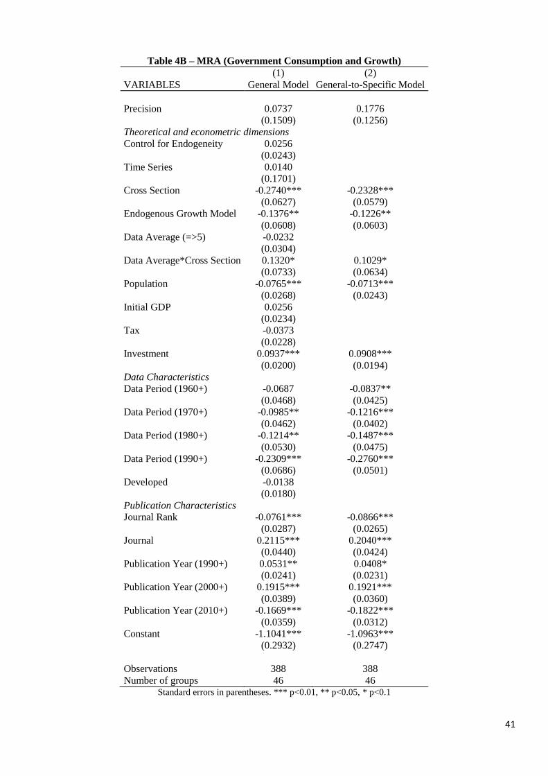
41

Table 4B – MRA (Government Consumption and Growth)

(1) (2)

VARIABLES General Model General-to-Specific Model

Precision 0.0737 0.1776

(0.1509) (0.1256)

Theoretical and econometric dimensions

Control for Endogeneity 0.0256

(0.0243)

Time Series 0.0140

(0.1701)

Cross Section -0.2740*** -0.2328***

(0.0627) (0.0579)

Endogenous Growth Model -0.1376** -0.1226**

(0.0608) (0.0603)

Data Average (=>5) -0.0232

(0.0304)

Data Average*Cross Section 0.1320* 0.1029*

(0.0733) (0.0634)

Population -0.0765*** -0.0713***

(0.0268) (0.0243)

Initial GDP 0.0256

(0.0234)

Tax -0.0373

(0.0228)

Investment 0.0937*** 0.0908***

(0.0200) (0.0194)

Data Characteristics

Data Period (1960+) -0.0687 -0.0837**

(0.0468) (0.0425)

Data Period (1970+) -0.0985** -0.1216***

(0.0462) (0.0402)

Data Period (1980+) -0.1214** -0.1487***

(0.0530) (0.0475)

Data Period (1990+) -0.2309*** -0.2760***

(0.0686) (0.0501)

Developed -0.0138

(0.0180)

Publication Characteristics

Journal Rank -0.0761*** -0.0866***

(0.0287) (0.0265)

Journal 0.2115*** 0.2040***

(0.0440) (0.0424)

Publication Year (1990+) 0.0531** 0.0408*

(0.0241) (0.0231)

Publication Year (2000+) 0.1915*** 0.1921***

(0.0389) (0.0360)

Publication Year (2010+) -0.1669*** -0.1822***

(0.0359) (0.0312)

Constant -1.1041*** -1.0963***

(0.2932) (0.2747)

Observations 388 388

Number of groups 46 46 Standard errors in parentheses. *** p<0.01, ** p<0.05, * p<0.1

42

Appendix – Overview of Methods

1. Partial Correlation Coefficients (PCCs)

PCCs measure the association between government expenditure and per-capita GDP growth. Given that they

are independent of the metrics used in measuring both independent and dependent variables, they allow for

the comparability of studies and reported effect-size estimates. They are mostly used in meta-analysis (see

e.g. Alptekin and Levine, 2012; Ugur; 2014; Benos and Zotou, 2014).

We use equations (A1) and (A2) to calculate a PCC and standard error, respectively, for each relevant effect-

size estimate reported by primary studies.

𝑟𝑖 =

𝑡𝑖

√𝑡𝑖2 + 𝑑𝑓𝑖

(A1)

and

𝑆𝐸𝑟𝑖 = √1 − 𝑟𝑖

2

𝑑𝑓𝑖

(A2)

𝑟𝑖 and 𝑆𝐸𝑟𝑖 represent PCC and its associated standard errors, respectively. 𝑆𝐸𝑟𝑖 represents variations due to

sampling error and its inverse is used as weight in the calculation of study-by-study fixed-effect weighted

averages. 𝑡𝑖 and 𝑑𝑓𝑖 represent 𝑡-value and degrees of freedom, respectively, associated with estimates reported

in primary studies.

2. Fixed Effect Weighted Means

We calculate FEEs using (A3) below.

�̅�𝐹𝐸𝐸 =

∑ 𝑟𝑖 (1

𝑆𝐸𝑟𝑖2 )

∑1

𝑆𝐸𝑟𝑖2

(A3)

�̅�𝐹𝐸𝐸 is the fixed effect weighted average and all other variables remain as explained before. FEEs account

for within-study variations by assigning higher weights to more precise estimates, and lower weights to less

precise estimates.

3. Bivariate meta-regressions

To estimate ‘genuine effect’ beyond publication selection bias, we draw on meta-regression analysis (MRA)

models proposed and developed by Stanley (2008) and Stanley and Doucouliagos (2012, 2014). The

underpinning theoretical framework is that of Egger et al. (1997), who postulate that researchers with small

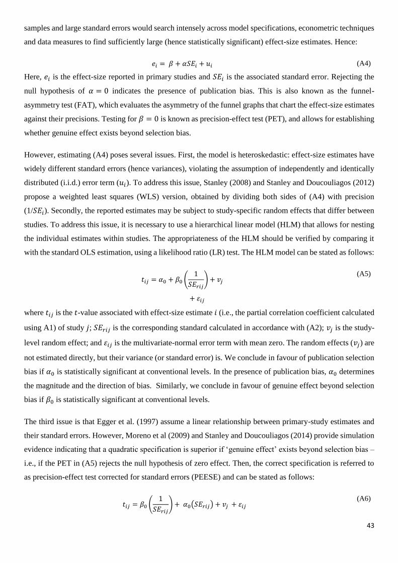
43

samples and large standard errors would search intensely across model specifications, econometric techniques

and data measures to find sufficiently large (hence statistically significant) effect-size estimates. Hence:

𝑒𝑖 = 𝛽 + 𝛼𝑆𝐸𝑖 + 𝑢𝑖 (A4)

Here, 𝑒𝑖 is the effect-size reported in primary studies and 𝑆𝐸𝑖 is the associated standard error. Rejecting the

null hypothesis of 𝛼 = 0 indicates the presence of publication bias. This is also known as the funnel-

asymmetry test (FAT), which evaluates the asymmetry of the funnel graphs that chart the effect-size estimates

against their precisions. Testing for 𝛽 = 0 is known as precision-effect test (PET), and allows for establishing

whether genuine effect exists beyond selection bias.

However, estimating (A4) poses several issues. First, the model is heteroskedastic: effect-size estimates have

widely different standard errors (hence variances), violating the assumption of independently and identically

distributed (i.i.d.) error term (𝑢𝑖). To address this issue, Stanley (2008) and Stanley and Doucouliagos (2012)

propose a weighted least squares (WLS) version, obtained by dividing both sides of (A4) with precision

(1/𝑆𝐸𝑖). Secondly, the reported estimates may be subject to study-specific random effects that differ between

studies. To address this issue, it is necessary to use a hierarchical linear model (HLM) that allows for nesting

the individual estimates within studies. The appropriateness of the HLM should be verified by comparing it

with the standard OLS estimation, using a likelihood ratio (LR) test. The HLM model can be stated as follows:

𝑡𝑖𝑗 = 𝛼0 + 𝛽0 (

1

𝑆𝐸𝑟𝑖𝑗) + 𝑣𝑗

+ 𝜀𝑖𝑗

(A5)

where 𝑡𝑖𝑗 is the 𝑡-value associated with effect-size estimate 𝑖 (i.e., the partial correlation coefficient calculated

using A1) of study 𝑗; 𝑆𝐸𝑟𝑖𝑗 is the corresponding standard calculated in accordance with (A2); 𝑣𝑗 is the study-

level random effect; and 𝜀𝑖𝑗 is the multivariate-normal error term with mean zero. The random effects (𝑣𝑗) are

not estimated directly, but their variance (or standard error) is. We conclude in favour of publication selection

bias if 𝛼0 is statistically significant at conventional levels. In the presence of publication bias, 𝛼0 determines

the magnitude and the direction of bias. Similarly, we conclude in favour of genuine effect beyond selection

bias if 𝛽0 is statistically significant at conventional levels.

The third issue is that Egger et al. (1997) assume a linear relationship between primary-study estimates and

their standard errors. However, Moreno et al (2009) and Stanley and Doucouliagos (2014) provide simulation

evidence indicating that a quadratic specification is superior if ‘genuine effect’ exists beyond selection bias –

i.e., if the PET in (A5) rejects the null hypothesis of zero effect. Then, the correct specification is referred to

as precision-effect test corrected for standard errors (PEESE) and can be stated as follows:

𝑡𝑖𝑗 = 𝛽0 (

1

𝑆𝐸𝑟𝑖𝑗) + 𝛼0(𝑆𝐸𝑟𝑖𝑗) + 𝑣𝑗 + 𝜀𝑖𝑗

(A6)

44

Given that study-level random effects may be observed at the intercept or slope levels or both, we establish

which type of HML is appropriate using LR tests, where the null hypothesis is that the preferred

specification is nested within the comparator specification. Therefore, we estimate HLMs with random-

intercepts only and HLMs with random intercepts and random slopes; and test whether the latter are nested

within the former.

4. Multivariate Meta-Regression Model (MRM)

To address the issues of heterogeneity, we estimate a multivariate hierarchical meta-regression model

specified in (A7) below.

𝑡𝑗𝑖 = 𝛼0 + 𝛽0 (

1

𝑆𝐸𝑗𝑟𝑖) + ∑ 𝛽𝑘

(𝑍𝑘𝑖)

𝑆𝐸𝑗𝑟𝑖+ 𝑣𝑗 + 𝜀𝑖𝑗

(A7)

Here, 𝑡𝑗𝑖 is the 𝑖th 𝑡-value from the 𝑗th study, while 𝑍𝑘𝑖 is a 𝑘 × 1 vector of moderator variables that capture

the observable sources of heterogeneity in the government size-growth evidence base.

To minimise the risk of multicollinearity and over-fitting, we estimate (A7) through a general-to-specific

estimation routine, whereby we omit the most insignificant variables (variables associated with the largest p-

values) one at a time until all remaining covariates are statistically significant. We present the findings from

the specific and general models side by side to: (a) establish the extent of congruence between the significant

moderating factors; and (ii) identify the range of moderating variables that do not affect the variation in the

evidence base.