Does Household Finance Affect the Political Process

Does Household Finance Affect the Political Process? Evidence

from Voter Turnout During a Housing Crisis*

W. Ben McCartney†

This Version: February, 2020Click here for the latest version

Abstract

I examine the effect of house price declines on voter participation using a novel person-level paneldataset. Contrary to what the “angry voter hypothesis” predicts, I find that a ten percent declinein local house prices decreases the participation rate of the average mortgaged homeowner by1.6 percentage points. Consistent with a financial distress channel, house price declines have noeffects on renters and particularly severe effects on highly leveraged households. My findingsare consistent with the existence of a feedback loop between financial distress and inequalityoperating through voter participation.

JEL Classification: D10, D72, H31, R20

Keywords: Household Finance, Financial Distress, Mortgages, Voter Participation, Elections

*This is a revised version of my job market paper, “Household Financial Distress and Voter Participation”. I am incred-ibly grateful to my committee: Manju Puri (chair), Manuel Adelino, Ronnie Chatterji, John Graham, and David Robinsonfor their feedback and support. The paper also benefited from comments and suggestions from Pat Bayer, Alon Brav, AnnaCieslak, Sergio Correia, Mara Faccio, Simon Gervais, Jillian Grennan, Huseyin Gulen, Isaac Hacamo, David Kaczan,Cam Harvey, Song Ma, Hugh Macartney, Adriano Rampini, Basil Williams, Ming Yang, and seminar participants at theFuqua Finance Brownbag, the Duke Political Science Graduate Student Colloquium, Auburn University (Harbert), RiceUniversity (Jones), Syracuse University (Whitman), the College of William & Mary (Mason), Baruch College (Newman),the Federal Reserve Board, the Federal Reserve Bank of Philadelphia, Purdue University (Krannert), Indiana University(Kelley), and the NYU Conference on Household Finance. All errors are my own.

†Purdue University, Krannert School of Management. Email: [email protected].

1

Electronic copy available at: https://ssrn.com/abstract=3068596

https://papers.ssrn.com/sol3/papers.cfm?abstract_id=3068596

1 Introduction

In democracies, the policymakers who write the legislation, implement the policies, and manage the

institutions are not randomly assigned, but rather elected by the very households they have affected

in the past and will affect in the future. These policymakers significantly influence the financial well-

being of their constituents.1 However, our understanding of the inverse – how households’ financial

situations affect who the policymakers are and the decisions they make – is limited. Furthermore,

elected leaders represent the average voter, not the average constituent, so who participates in elec-

tions matters (Cascio and Washington, 2013; Fujiwara, 2015; Miller, 2008). Consequently, identify-

ing whether financially distressed households are especially likely or unlikely to vote has important

implications for the direction of public policy, wealth and income inequality, and the legitimacy of

American democracy.

The effects of negative financial shocks on voter participation are theoretically ambiguous (Rosen-

stone, 1982). On the one hand, voters hit by negative shocks may go to the polls seeking either to

bring about a regime change or to punish incumbents – this hypothesis is colloquially known as the

“angry voter hypothesis.” On the other hand, affected households might be less likely to participate

if these shocks cause emotional or financial distress. It is important to remember that voting is not a

quick activity that occurs just on election day. Voters must learn about the candidates and decide for

whom to vote, make sure they know where to vote, and then get to the polling place and stand in line

for, in some cases, hours. Finally, there may be no relationship if voters do not blame incumbents, do

not view voting as a way to affect change, or vote for reasons of ideology or civic responsibility that

are unaffected by negative financial shocks.

For many households, their home is their most valuable asset and their mortgage their largest

liability. Consequently, large, negative shocks to house prices, like those observed during the Great

Recession, serve as a meaningful shock to the financial well-being of households and an appropriate

setting to determine whether, and how, economic distress affects participation. To test if house

price declines increase or decrease participation, I merge the voter rolls and deeds records of North

Carolina to build a novel individual-level panel dataset. All together, I know the name and address

of all registered voters in the state, whether or not they participated in each election, what happened

to their neighborhood’s house prices leading up to each election, whether they rented or owned, and,

if they owned, the details of their outstanding mortgage.

I identify the effects of home price declines on voter participation by exploiting variation in home

price declines across zip codes and over time in North Carolina during the years of the Great Re-

cession. Using this identification strategy on the novel dataset described above, I find that potential

1In the real estate space alone, consider, the effects of the homebuyer tax credit (Berger et al., 2016; Floetotto et al.,2016), the mortgage interest deduction (Glaeser and Shapiro, 2003; Hilber and Turner, 2014; Sommer and Sullivan, 2018),the government sponsored enterprises (GSEs) Fannie Mae and Freddie Mac (Elenev et al., 2016; Frame et al., 2015; Geteand Zecchetto, 2017), the conforming loan limit (Adelino et al., 2012; DeFusco and Paciorek, 2017), collateral requirements(Agarwal et al.; DeFusco et al., 2017; Gupta and Hansman, 2019), the now abolished policy of redlining (Appel and Nicker-son, 2016), rules, or a lack thereof, for lenders (Di Maggio and Kermani, 2017; Favara and Imbs, 2015), HAMP and HARP(Ganong and Noel, 2017; Keys et al., 2016), and, looking to the future, affordable housing policies (Autor et al., 2014;Diamond and McQuade, 2019; Favilukis et al., 2018), among many other policies and many other papers.

2


voters who experienced larger negative home value shocks were less likely to vote in elections.2 To

overcome the endogeneity concern that house price falls might be spuriously correlated with lower

turnout, I include in my models a battery of individual-level controls, including age, race, ethnicity,

sex, state of birth, and year of registration. Because there are likely other time invariant factors that

influence baseline participation rates, I also control for each person’s participation decisions in the

two pre-recession elections of 2008. All of these variables are observed and modeled at the individual-

level to help me overcome the limitations of ecological inference (King, 2013). Further, I include in

all specifications county-by-election and party affiliation-by-election fixed effects. These fixed effects

soak up regional and political party differences in participation and the fact that these differences

likely vary over time. Finally, because I can follow individuals over time, I am also able to estimate

models that include voter fixed effects. I find that a ten percent decline in home values caused on

average a 0.8 percentage point drop in participation likelihood, meaning voter participation would

have been 1.2 percent higher had there been no collapse in house prices.

I next allow the affects of house price falls to be non-linear and find that it is large house price

falls, especially, that affect voter participation. Motivated by this finding, I use a conservative back of

the envelope estimation to show that house price declines can explain approximately 36,000 absten-

tions in North Carolina during the 2010 and 2012 election cycles, or an average of 9,000 abstentions

per election. For context, Barack Obama received 14,177 more North Carolina votes than John Mc-

Cain in the 2008 presidential election.

Models with voter fixed effects help rule that my results are driven by unobserved differences

between people living in zip codes where house price falls were severe and people living in zip codes

where house price declines were mild. And the richness of the data also allows me to use other

tests that rely on different identifying assumptions for validity. Specifically, I use a difference-in-

differences design and interact home value declines with homeowner status. I group potential voters

into one of three types: renters, owners without mortgages, and owners with mortgages. If home

value declines were causally lowering voter turnout, and not simply correlated with, for example,

negative employment shocks or lower political advertisement spending, we would expect to see that

home value declines affect participation most for homeowners with mortgages and least for renters.

This is exactly what I find. Within county-by-election and party-by-election, and controlling for the

same battery of control variables as before, I find that renters and homeowners without mortgages

are not significantly affected by a ten percent decline in home value while households with mortgages

are 1.6 percentage points less likely to participate. A remaining identification concern is that renters

and homeowners experienced different income and employment shocks. I cannot observe these in my

dataset, so I turn to the Panel Study of Income Dynamics (PSID) and show that in North Carolina the

effects of the recession on the employment and income of renters was statistically indistinguishable

from its effects on homeowners.

I next explore whether the effects of house price falls differ across households’ expected equity

position. I do this in four ways. First, I test whether the voter turnout among households who

2In this paper, I focus my attention on the 2010 primary, 2010 general, 2012 primary, and 2012 general elections.

3


moved in prior to 2003 is less affected by home price declines than the turnout of their neighbors

who moved in between 2003 and 2007. Since households who purchased during the boom are likely

different than households who purchased before it, I next focus only on households who purchased

during the boom and compare high-CLTV (CLTVs at purchase of strictly greater than 80%) to low-

CLTV purchases (CLTVs strictly greater than 0% or less than or equal to 80%). Third, using the

sample of only high-CLTV purchasers, I compare those who purchased during the boom to those who

purchased pre-boom. In all three cases, I find that households I expect are more highly leveraged at

the onset of the recession are especially less likely to participate in elections following home value

declines. Finally, I incorporate refinance activity and calculate a synthetic current LTV for every

household and find that near-underwater and especially underwater households are significantly

less likely to participate.

Lastly, I investigate if a lost wealth channel can explain the results or if financial distress caused

by the negative wealth shock is a more likely culprit. Assuming that households with low leverage

are less likely to be financially distressed as a result of house price declines (as suggested by the

work of Foote et al. (2008) and Foote et al. (2010)), my result that house price declines most severely

affect highly leveraged homeowners points to a financial distress / default risk channel, not a lost

wealth channel. Furthermore, by expanding the sample to include the 2014 and 2016 election cycles

and the house price appreciation that was occurring during this time period, I show that house price

increases do not affect voter participation, inconsistent with a pure level-of-wealth effects story.

To provide more evidence that financial distress matters, I present two relevant results. First,

I find that households whose polling place has changed since the last election cycle are especially

affected by falls in home values. Second, surveys conducted by the US Census find that, in the

general elections of 2010 and 2012, “too busy, conflicting schedule” was the most common answer

given by abstainers when asked why they did not vote.3 Overall, I propose that a distress channel,

where large house price drops cause households to become financially distressed, increasing their

opportunity cost of voting and tightening their resource constraints, is the most consistent with the

body of evidence I provide.

1.1 Contributions to the Literature

This paper contributes to four literatures. To the literature seeking to identify the effects of economic

adversity on voter participation and civic engagement I make three contributions. First, I use a

novel measure of economic adversity. The majority of papers in this literature measure distress

with unemployment or foreclosure (see, e.g., Burden and Wichowsky (2014); Cebula (2017); Estrada-

Correa and Johnson (2012); Hall et al. (2017)), so using house price declines allows me to estimate

the effect of a somewhat less extreme, but far more prevalent, kind of economic distress. Second,

and very importantly, given the prevalance of the “angry voter hypothesis” in today’s discourse, the

extant academic literature still has yet to reach a consensus on the first-order question of whether

distress increases (mobilization), decreases (withdrawal), or has no effect on voter participation.

3See, e.g., https://www.census.gov/data/tables/2012/demo/voting-and-registration/p20-568.html

4


https://www.census.gov/data/tables/2012/demo/voting-and-registration/p20-568.html

Third, by identifying an effect operating at the individual-level I can speak to which individuals,

specifically, participate more or less when hit by house price shocks / distress. Closely related to this

paper is Hall et al. (2017), who, also using individual-level data, examine the effects of foreclosure

on participation. While Hall et al. (2017) focus on those households that foreclosed, I explicitly drop

them, meaning that the samples used in the two papers are, by design, mutually exclusive and the

conclusions – that being foreclosed on decreases participation and experiencing mortgage distress

decreases participation – complementary.

Second, I contribute to the literature examining the real effects on households of negative shocks

to home values. Mian et al. (2013) highlight the role of debt and the importance of household eq-

uity in consumption and Baker (2018) further shows that negative income shocks are particularly

harmful to households with high debt to asset ratios. Bernstein (2015) finds that the implicit tax

on underwater households, households who owe more on their mortgage than their home is worth,

results in significant decreases to household labor supply. Those households that continue to work

do so for lower wages (Cunningham and Reed, 2013) because they are less likely to be able to relo-

cate to higher paying jobs (Brown and Matsa, 2016) and, more broadly, to avoid the double punch

of being both underwater and unemployed (Foote et al., 2008). The effects on the broader economy

are also severe, as highly leveraged households are less likely to start firms (Schmalz et al., 2017)

and less likely to successfully pursue innovation projects (Bernstein et al., 2017). Melzer (2017),

again because of the implicit taxes of debt overhang, documents that underwater households cut

back on home improvements. And finally, the health and well-being of homeowners also deterio-

rates because of mortgage distress (Currie and Tekin, 2015; Deaton, 2012). I contribute evidence

that negative home value shocks also affect voter participation, a critically important activity for a

well-functioning democracy.

Third, my results add to the conversation about the future directions of US housing policy by

demonstrating that housing policy and voter participation are perhaps more tightly linked than we

knew. Policymakers citing the benefits of the homeownership society (see, e.g., Sodini et al. (2016))

should keep in mind that homeownership at any expense might adversely affect one of the very

outcomes they hope to encourage – voter participation and, more broadly, civic engagement (Ekman

and Amnå, 2012). Also, policies limiting CLTV ratios might lead to higher voter participation rates

in market downturns (see Cerutti et al. (2017) and DeFusco et al. (2017) for recent papers discussing

these types of policies). And finally, Agarwal et al. (2017) show that the Home Affordable Modification

Program (HAMP) was associated with lower rates of foreclosure, milder house price declines, and

increases in durable spending. To their findings, I add novel evidence that HAMP, and programs like

it, might also serve to strengthen communities by halting the decline in voter participation and civic

engagement that follows collapses in home values.

Finally, my results provide suggestive evidence of a mechanism linking inequality and politics in

democracies (see the massive literature spawned by Bartels (2008), and Acemoglu et al. (2015) for

a review). The link between these two trends is still poorly understood (Feigenbaum et al., 2018;

Gimpelson and Treisman, 2018; Solt, 2008), but we have reason to believe that policy making fails

5


to reflect the preferences of those unable to vote (Cascio and Washington, 2013; Chattopadhyay and

Duflo, 2004; Fujiwara, 2015; Miller, 2008). The concern this paper raises, then, is that those voters

less likely to vote are exactly those suffering from financial distress and who might benefit from

policies of wealth redistribution or the support of their representatives (see, for example, Agarwal

et al. (2018)). This paper finds that during times of economic hardship financially secure citizens

have a higher vote share and can use that to elect policymakers who will change the rules of the

game for their private benefit. In short, this paper’s final contribution is evidence consistent with

the concern of a feedback loop between household financial distress and inequality that operates

through a voter participation channel.

2 Data

2.1 Data Sources

2.1.1 North Carolina Voter Files

I use the North Carolina voter files because they are free to use, publicly available, and cover

pre-recession elections.4 These data are provided by the North Carolina State Board of Elections

(NCSBE) and come in two parts. The history file is at the individual person level and lists, for every

person who has ever voted in any North Carolina election since 2008, all of the elections they have

participated in. To be eligible to vote in North Carolina elections, residents of the state must com-

plete a voter registration application. The second set of files, the snapshot files, covers the universe

of registered voters. These files are published periodically by the Board of Elections, typically before

important elections. Each snapshot includes the name and address, political party affiliation, year

of registration, age, race, sex, and US state of birth (if applicable) of every registered voter. These

two datasets can be merged using a person-level linking variable provided by the NCSBE. The only

limitation of this identifying variable is that it is defined at the person-by-address level. That is,

anyone who moves to a new location is assigned a new identifier. The NCSBE also publishes on its

website a list of each precinct’s polling place for every election. With this information, I can identify

each individual’s closest polling place and if this location changes from one election to the next.

The voter files from the NCSBE have several excellent characteristics for studying the effects of

home value declines on participation. First, the population covered by the voter files is the complete

universe of registered voters in North Carolina. No counties, demographic groups, or time periods

since the data began are missing or underrepresented. Second, the overwhelming majority of the

variables are nonmissing for all individuals. Third, and most importantly, the dataset is incredibly

clean. As the official voter file for all of North Carolina’s elections, the incidence of data entry errors,

especially for the name and address fields, is near zero.

In this paper, I focus on the 2008, 2010, and 2012 general elections and their primaries. While

the North Carolina voter files do include participation in every local and special election, I omit them

4https://dl.ncsbe.gov/index.html

6


https://dl.ncsbe.gov/index.html

from this study for two reasons. First, these elections vary in economic importance and meaning,

especially when compared with the federal elections. Second, in many cases, identifying the list of

voters eligible to vote in a given local election is non-trivial. In contrast, I know that every registered

voter is eligible to vote in the federal elections. Thus, by focusing on the six federal elections between

2008 and 2012, I ensure uniform tops-of-the-ballot and common eligibility for all voters in the state.5

2.1.2 Housing Data

The housing data I use is sourced, originally, from two places. Each county has both a recorder’s

office that keeps a record of all legal documents affecting title to real property in the county and an

assessor’s office that tracks the owner and value of all property in the county.6 These data are also

publicly available and cleaned and published formerly by DataQuick and now by CoreLogic. As with

the voter data, this data is used for official purposes, namely property taxes, and is consequently

very clean.

A great deal of information is obtainable from the deeds records. The assessor files list the com-

plete address of every property in the state, the full name of the current owner, when the property

was last purchased, and how much it was purchased for (though purchase price is sometimes miss-

ing). The recorder’s office tracks the liens against the property. Specifically, I know the size of each

mortgage, including second and third, piggyback, loans. This allows me to construct the combined

loan-to-value (CLTV) ratio of the purchase loan. For some counties, the deeds data goes back as far as

1990. Counties are then added to the dataset as time passes, and by 2006 almost all of the counties

are covered by CoreLogic. CoreLogic, conveniently, has an identifier variable that allows for a many-

to-one merge between all the mortgage loans made against a property (from the recorder’s office) and

the property (from the assessor’s office). To clarify, I know the current owner of every property in

North Carolina. I also know the previous owner and the terms of the outstanding mortgage for those

properties that were purchased after CoreLogic’s coverage of the county began.

2.1.3 Zillow Home Values

The third data source is the Zillow Real Estate Research website. To measure local housing mar-

ket conditions, I use the Zillow historical monthly zip code median home price.7 The Zillow Home

Value Index (ZHVI) is, per their website, a “smoothed, seasonally adjusted measure of the median

estimated home value across a given region and housing type.”8 It is not a repeat-sales index, but is

highly correlated with the Case-Shiller index, a commonly used repeat-sales index (Guerrieri et al.,

2013). During the time period I focus on in this paper, 2008-2012, Zillow publishes a ZHVI for 484 of

the 808 zip codes in North Carolina, covering approximately 87% of the population (see Figure 1).

5For an examination of voter participation in local elections see Hall and Yoder (2018).6For examples of the raw data, visit the Durham county records search, http://property.spatialest.com/nc/durham/, the

Wake county real estate property search, http://services.wakegov.com/realestate/, and the Wake county register of deeds,http://services.wakegov.com/booksweb/genextsearch.aspx

7The data can be downloaded here: https://www.zillow.com/research/data/8For more information about the measure see: https://www.zillow.com/research/zhvi-methodology-6032/

7


http://property.spatialest.com/nc/durham/

http://services.wakegov.com/realestate/

http://services.wakegov.com/booksweb/genextsearch.aspx

https://www.zillow.com/research/data/

https://www.zillow.com/research/zhvi-methodology-6032/

2.1.4 North Carolina

North Carolina is a state particularly well suited for this study. Compared to the United States as a

whole, North Carolina is remarkably representative. In 2012, North Carolina was slightly less white

(69.9% vs. 73.9%), was more likely to live in an owner-occupied housing unit (65.4% vs 63.9%), and

had a lower median income (45k vs 51k). Politically, the state is right in the middle of the spectrum.

In the 2008 and 2012 presidential elections, the state’s popular vote share for Obama was 49.7%

and 48.4%, respectively, compared to 52.9% and 51.1% across the country. North Carolina, perhaps

because it is a swing state, has higher participation than the rest of the country, 66%, 40%, and 65%

compared to 62%, 41%, and 59% in the 2008, 2010, and 2012 general elections, respectively. House

prices in North Carolina are lower than in the rest of the United States, and the fall during the bust

was less severe. Specifically, as of March 2009, the median house price in North Carolina was $148k

compared to $171k in the United States. House prices fell in North Carolina to a low of $134k in

January of 2012 and did not begin to recover until the summer of 2013. In the United States, the low

occurred in March 2012 at $148k.9

Even in its own right, regardless of how it compares to the rest of the country, North Carolina is

important. In 2010, the state had 9.5 million citizens and a GDP of approximately $400 billion. It

has been a battleground state since at least the 2008 presidential election when Obama received just

14,177 more votes than McCain out of 4,310,789 votes cast. Midterm elections, too, are competitive.

In the 2014 senatorial race, the Republican Thom Tillis received 45,608 more votes than the incum-

bent Democrat Kay Hagan. Most recently, the 2016 governor’s race was decided by just 10,277 votes

when Roy Cooper (D) defeated the incumbent Pat McCrory (R) despite the state voting for Trump in

the Presidential election.

2.2 Dataset Construction

I merge these three datasets – the voter rolls, deeds records, and zillow home value index – to create

a novel, individual-level panel dataset. I start with the North Carolina voter sample which includes

7.4 million unique voter-by-address individuals over the period 2008 to 2012. Because the voter

identification number is tied to the county and because names are non-unique, I cannot follow voters

as they move across the state. The dataset, therefore uses this voter-by-address identifier as its panel

variable. Next, I match individuals in the voter rolls to property owners in the deeds data using a

merge described in detail in Appenix B. My algorithm works well, classifying 62% of the registered

voters in North Carolina as homeowners while American FactFinder classifies 65% of the population

of North Carolina as homeowners.

The final sample makes two restrictions on this universe of voters and deedholders. First, I

drop zip codes for which Zillow does not publish median house prices. This reduces the sample to

5.3 million unique voter-by-address individuals, approximately 3.1 million (or 59%) of whom own

homes and 1.9 million of whom have mortgages. Second, I include only voters who were eligible

9These numbers from Tables DP-1 and S1902 from American FactFinder, Ballotpedia, and Zillow Research. For morecomparisons between NC and the other 50 states see Table A1.

8


https://factfinder.census.gov/faces/nav/jsf/pages/index.xhtml

https://ballotpedia.org/Main_Page

https://www.zillow.com/home-values/

to vote in all of the federal elections between 2008 and 2012. Since I cannot follow voters if they

move, this restriction means the sample includes only those voters who stay put during the whole

sample. I enforce this restriction on the sample for two reasons. One, by observing whether each

voter participated in the two pre-crisis period elections, I am able to control for each voter’s baseline

participation rate. Two, using this sample focuses the results to come as cleanly as possible on people

being affected by house price falls and nothing else. For example, households already planning to

move or beginning to default on their loans at the time of the election will be omitted from the sample

since it restricts itself to just those would-be voters who stay at the same address over the entire time

series. These are interesting and economically important groups, but I want my empirical tests to

speak to the effect of house price declines, not migration or foreclosure.10

2.3 Summary Statistics

The final sample has 3.2 million unique voter-by-address individuals, 2.4 million (or 74%) of whom

own their homes and 1.5 million of whom have mortgages. Table A2 describes the demographics of

the sample and Table A3 presents participation rates. The bottom two panels of Table A3 preview the

main finding of the paper. In the 2010 and 2012 elections, households experiencing large house price

declines are unconditionally less likely to vote, as are highly leveraged and, especially, underwater

households.

[FIGURE 1 HERE]

Between 2008 and 2012, house prices fell substantially across the state of North Carolina. Lead-

ing into the general election of 2008, only 14% of eligible voters experienced local house price falls

of more than 5%. By November 2010, the month of the 2010 general election, almost everybody was

experiencing some sort of house price decline including 24% a fall of more than 10%. Figure 1 il-

lustrates the house price falls between the 2008 and 2010 general election in zip codes across North

Carolina. Importantly, the home value declines are both meaningful and varied. And, as shown in

Table A4, the variation occurs even at a local, county level.

That is, it is not the case that all of the home value declines were concentrated in one or two areas.

Rather within any given part of the state there were some zip codes where home value declines were

significant and some zip codes where the falls were milder. Furthermore, the declines also vary

across time. For example, in Mecklenburg County (Charlotte), 10% of registered voters experienced

house price falls of 14.59% or greater in the 24 months leading up to the 2010 general election

while 25% of voters, in the same county, experienced house price falls of less than 9.57%. In 2012,

while the average Mecklenburg County voter’s house price declined by only 5.69% (compared to

10.86% in 2010), there was still very large dispersion with the 10th percentile voter experiencing a

slight increase in house prices and the 90th percentile voter living in a zip code where house prices

10For work examining the effects of foreclosure on participation see Hall et al. (2017) who find that foreclosed on votersare less likely to turn out to vote.

9


fell by 15%. By using several elections of data to estimate the effect of house price falls on voter

participation, I can utilize variation both across space and across time, all within county.

3 A First Test for the Effects of House Price Falls

3.1 Description of the Identification Strategy

To identify the effects of house price falls on voter participation, I exploit the varied timings and

magnitudes of house price falls across the state of North Carolina in the years following the 2008

financial crisis. The key identifying assumption is that this variation in house price falls leading up

to the 2010 midterm, 2010 general, 2012 midterm, and 2012 general elections was, conditional on

a number of control variables and fixed effects, as if randomly assigned. To fix ideas, consider the

sparsest specification of the model I will estimate in this paper:

Participatedit =β×% Fall in Home Valuezt +County-by-Electionct, (1)

where i indexes voters, t indexes elections, z indexes zip codes, and c indexes counties. Participatedit

is a dummy equal to 100 if voter i participated in election t and zero otherwise.11 The variable of

interest, % Fall in Home Valuezt, is the percent decrease in the median home value in zip code z

in the twenty-four months leading up to election t. The model also includes fixed effects for each

county-by-election. Because the federal elections vary in importance, baseline participation rates

vary tremendously across them. It is therefore crucial to compare only voter participation decisions

within elections. Furthermore, there are a number of reasons participation might vary across the

state, including, for example, differences in campaign spending and ad buys, whether important local

elections are also on the ballot, and changes in other sectors of the macroeconomy. These sources of

variation could be controlled for with just election fixed effects and county fixed effects. But, since

the differences in elections also vary across counties and the differences between counties are not

constant over time, I include a county-by-election fixed effect. This forces as much of the variation as

possible to come from differences in local home price changes.

Even within county, though, individuals’ zip-codes are not randomly assigned. To ensure this

does not drive my results, I first leverage the panel nature of the dataset and the fact that in most

of the state, house prices did not begin falling in earnest until after the 2008 election. This allows

me to take participation in the 2008 midterm and 2008 general elections as a pre-treatment control

variable. Many of the individual-level characteristics we might worry cause sorting across zip codes

will be reflected in these two control variables.

Next, I include a battery of control variables and fixed effects.12 Specifically, I include variables

controlling for each individual’s age, race, ethnicity, sex, state of birth, registration year, and party

affiliation. By including these control variables in my models, I absorb many of the observable char-

11I use 100, instead of 1, so the coefficient estimates can be easily interpreted in percentage point terms.12The estimation of models with high dimensional fixed effects is made possible by Correia (2017).

10


acteristics that we know to be correlated with voter turnout and, perhaps, sorting across zip codes. I

also include party affiliation-by-election fixed effects. This absorbs any differences in common drivers

of voters of different parties to participate in each election. For example, it might be that voters affil-

iated with the party out of power are more likely to participate in the midterm elections. If they also

live in zip codes where house price declines were different than zip codes where voters of the other

party live, then my estimates of home value declines on participation would be biased.

Finally, in order to quash as much of the variation coming outside of house price declines (omit-

ted variables or endogenous sorting across zip codes), I include an individual-voter fixed effect. This

specification therefore identifies off of only variation in house prices across the time series since it

absorbs all time-invariant individual characteristics, even those that are unobservable to the econo-

metrician.

3.2 The Effects of Home Value Declines

[TABLE 1 HERE]

The first results of this paper are presented in Table 1. In column 1, I estimate a negative rela-

tionship between a fall in house prices and voter participation. Specifically, I find that a 10% decline

in local house prices makes the average voter 2.7 percentage points less likely to participate. Since

voters endogenously choose zip codes, the second specification includes three sets of controls. The

inclusion of these controls attenuates the affect of home value falls, but the effect still remains sta-

tistically significant at the 1% level and economically significant: a ten percent drop in house prices

causes a 1.3 percentage point decrease in participation likelihood. Model 3 adds party-by-election

fixed effects and model 4 includes the final control variable: a categorical variable for homeowner

status. Table 1 shows that these two models predict a drop in participation of 1.1% and 0.9% follow-

ing a ten percent decline in local home values leading up to a federal election. The final column of

this table removes all the individual-level controls and uses instead voter fixed effects and election

fixed effects. By including voter fixed effects, I control for all of the individual-level factors that are

constant over time and might affect participation, like career choice and education.

[TABLE 2 HERE]

I further explore the main finding, that house price drops decrease average voter participation

likelihood, in Table 2. Models 1 and 2 use the drop in house prices in the one year and four years lead-

ing up to the election, respectively, and the main result is robust to this modeling choice. Ultimately,

I use the drop in house prices occurring over the previous two years in my preferred specifications

because two years is the time between election cycles. The estimates from the third model mean we

can rule out that what matters is only if house prices fall, not the extent to which they drop. The

fourth model means the main result is not driven by just a few outlier zip codes that experienced

massive drops in house prices. Taken together, the results in Tables 1 and 2 show a negative rela-

tionship between house price falls and voter participation that becomes statistically significant once

house price falls approach 10%.

11


4 Limitations of Using Ecological Inferences

Extant work has used aggregate measures to reach conclusions about the effects of a variety of factors

on voter participation and about the effects of financial distress on many outcomes. This strategy is

appropriate if the goal is to determine, e.g., global drivers of global turnout, but is, except under very

special circumstances, inappropriate for identifying the mechanisms behind causal, individual-level

economic relationships. Since at least 1950, social science has known that ecological correlations

cannot be used as substitutes for individual correlations (Kramer, 1983; Robinson, 2009). Statisti-

cally, this is because the average within-area individual correlations are not identical to the total

individual correlation, as correlations between independent and dependent variables of interest are

generally smaller for relatively homogenous sub-groups than for the population at large.

For example, the main finding of this paper so far, that local house price declines cause lower

voter turnout, does little to explain why suffering a negative house price shock makes households

less likely to vote. It might well be that falls in local house prices cause some households to become

financially distressed and these distressed households stop participating. But a second possibility is

that house price declines have no effect on homeowners at all, but rather make home-buying, a time-

intensive activity, more attractive to renters, landlords, and investors, who choose to spend their

time doing this instead of voting. Or, thirdly, equity rich households may see house price declines

as evidence that the current political system is dysfunctional and not worth participating in. Yet

another possibility is that declines in house prices may equally affect everybody either because all

three of the mechanisms just described are relevant, or for some fourth mechanism. Perhaps house

price declines cause neighborhoods to work together to solve local problems brought about by large

negative house price shocks and they spend their time and energy doing that instead of voting.

A fifth possibility is that local house price declines alter the neighborhood’s population of eligible

voters. For example, it might be that as house prices fall, new, younger homeowners move in. If

younger people are less likely to vote, then that would explain the drop in participation. Studies that

use area-level tests might include a variable for share of people within a certain age range, or share

of people that have recently moved in, to help control for this story. But because those strategies do

not see who specifically is not voting, we cannot be sure that controlling for area-level demographics

does what we need. Consider for example the possibility that new people moving into a neighborhood

directly affect those already living there by making them less engaged with their communities. In

this case, the set of people not voting might be people of different ages or races than the newcomers.

The ramifications of these two alternative stories are very different, but an area-level test cannot

disentangle them.

The implications of these six stories on the question of whether financial distress and households’

ex ante financing decisions matter for how governments are formed and what policies they implement

are very different. If house price declines differentially affect people with different preferences for

the role of government and the projects governments undertake, then it matters who is not voting

because of those house price declines. In general, making correct inferences about individual-level

causal effects based on observed aggregate correlations is infeasible. For more theory see King (2013)

12


and for discussions in other empirical settings see, e.g., Arceneaux (2003) and Adelino et al. (2016).

5 Renters, Homeowners, and Expected Equity Positions

In this section I classify households by how likely it is that home value declines affect them. Specifi-

cally, I group individuals into renters, homeowners with mortgages, and homeowners without mort-

gages. I then divide homeowners based on three proxies for expected equity position – recent pur-

chase vs old purchase, recent high-CLTV purchase vs recent low-CLTV purchase, and recent high-

CLTV purchase vs old high-CLTV purchase. These models are all estimated using an equation of the

following form:

Participatedit = γ×Homeowneri ×% Fall in Home Valuezt

+δ×Homeowneri +Controlsi ×Θ+County-by-Electionct +Zip-by-Electionzt.(2)

The identifying assumption is that many of the unobservable characteristics that lead individuals to

choose specific zip codes within the county will be shared by individuals who own their homes and

those that rent them, or by individuals that I expect to have low equity in their homes and those that

I expect are less leveraged. Furthermore, since they are living in the same zip code, these individuals

share exposure to any other potentially confounding local shocks. The only difference, then, is their

home-ownership status or expected equity position and, consequently, how economically important a

drop in house prices is.

Comparing renters and owners is natural when exploring the effects of changing home values.

For most homeowners in the United States, housing is the largest asset on their balance sheet, and

their mortgages are their largest liabilities. Large negative shocks to home values are consequently

likely to be especially economically important and salient for homeowners as compared to renters.

Renters may care about housing prices to the extent that they value the option of purchasing a

home, but the immediate effects of home price shocks will be felt largely by homeowners. The results

of this test will also speak to potential channels. If I find that renters and homeowners are similarly

affected by house price falls, the set of possible mechanisms through which house price falls decrease

participation stays relatively large. If, on the other hand, I do find differential effects, then that not

only suggests the validity of the identified results, but also points to a financial distress or lost-wealth

channel.

Further motivated by the idea that households with substantial equity in their homes are less

likely to be materially affected by house price declines, my second major sample split compares

homeowners with different expected equity positions. There are two bases for this assumption. First,

Foote et al. (2008) and Foote et al. (2010) find that falling house prices and some second negative

shock are the key drivers of foreclosure. A decline in house prices that pushes households underwater

is a necessary condition for default. Households whose leverage was higher to begin with are more

likely to be pushed underwater by a decline in house prices than their equity rich neighbors. Second,

if highly-leveraged households were expecting to cash-out refinance in the future as house prices

13


increased, then learning that they cannot because their home’s value has declined might lead to

real, negative effects.

In light of the mortgage distress many households experienced during the recession, the Panel

Study of Income Dynamics (PSID) survey added questions A27F6 and A27G that asked households

how likely they are to fall behind on their mortgage. I use survey responses to questions A20 and A24

to determine if households are underwater. Of PSID respondents, 37% of underwater homeowners

in the 2009 survey say they are worried about falling behind compared to only 11% of homeowners

who are not underwater. In 2011, 32% and 8%, respectively, are concerned. Furthermore, within

households over time, being underwater is correlated with a .6 point increase in respondent’s K-6

non-specific psychological distress score, a score out of 24, and a 21 percent increase in receiving

financial help from family and friends (G44). These results are not conclusive evidence, but are

consistent with the theoretical prediction that highly leveraged households experiencing negative

house price shocks face more severe consequences from that decline in home values than their equity

rich neighbors.

5.1 Renters, Homeowners without Mortgages, and Homeowners with Mortgages

[TABLE 3 HERE]

The first four specifications in Table 3 are variations of Equation 2, comparing renters, homeown-

ers without mortgages, and homeowners with mortgages.13 The first two models compare renters,

those least likely to be materially affected by a decline in house prices, to owners with mortgages,

those most likely to be affected. In the first specification, I find that renters are completely unaffected

by home value declines controlling for a number of demographic variables, and county-by-election

and party affiliation-by-election fixed effects.14 Homeowners with mortgages, though, are 1.4 per-

centage points less likely to vote following a ten percent decline in local house prices. Model 2 uses a

zip-by-election fixed effect instead of a county-by-election one which precludes the identification of a

main effect, but further forces the identification to come not from differences across zip codes within

counties but just from the differential effect of house price falls on homeowners with mortgages as

compared to renters.

Models 3 and 4 add in the third group, homeowners without a mortgage. These three groups

are mutually exclusive and span the population of registered voters. I find that households without

mortgages are also unaffected by home value declines. Both of these models include the full set of

controls and, as with models 1 and 2, differ only in their use of county-by-election or zip-by-election

fixed effect. For more specifications that introduce the control variables and fixed effects as in Table

1, see Table A6.

The final three columns of Table 3 split the sample into renters, owners without mortgages, and

13Table A5 presents summary stats for these these three samples.14Note that average rental prices in North Carolina were very steady over the time series, even during the housing crisis

(see American Fact Finder Table CP04). There is variation in the level of rental prices across counties and zip codes, butthis variation is absorbed by county and zip code fixed effects, respectively.

14


mortgaged owners and then re-run the fifth specification from Table 1 that substitutes an individual

person fixed effect for the control variables. In these results, I find that mortgaged homeowners are

the only group affected by house price falls. Specifically, a ten percent higher drop in house prices

causes a 1.1 percentage point decline in the average mortgaged homeowner’s participation likelihood.

The results of this table make three points. First, the relationships illustrated in Tables 1 and

2 are driven especially by homeowners with mortgages, not homeowners without mortgages and

not renters. Second, people sorting into zip codes where house prices fell dramatically cannot alone

explain the results in Section 3.2. That is, if whatever caused people to choose the zip code in the

first place was correlated with decreased voter participation as a result of home price declines, we

would expect to see this effect in everybody that chose the zip code, renters and homeowners with

and without outstanding mortgages. Third, other alternative hypotheses that propose some shock

that affects both participation and house prices now also have to explain why that shock only affects

homeowners with mortgages.

5.2 Expected Equity Position

The richness and size of the dataset means I can be aggressive in creating subsamples to help rule

out some of these possible alternative hypotheses. In this section, I use three different proxies for

expected equity position and present the results of the tests in Table 4.

[TABLE 4 HERE]

The first test uses two subsamples of all homeowners: those who purchased their homes between

1996 and 2002 and those who purchased their homes between 2003 and 2007. Since homeowners

who purchased their homes in the first time period had longer to accumulate equity in their homes,

they should be less affected by house price declines. I find that while all of these homeowners are

less likely to vote following declines in house prices, the effect is approximately three times stronger

for homeowners who purchased in the period immediately preceding the crisis.

In specifications 3 and 4, I limit the sample to just homeowners with mortgages who purchased

between 2003 and 2007. High-CLTV purchase individuals are defined as those who put strictly

less than 20% down. The control group, those less likely to be adversely affected by house price

declines, are homeowners who put down more than 20%, but strictly less than 100% (i.e., they took

out some kind of mortgage). The advantage of this test is that I can be more confident that my control

group provides a reasonable counterfactual for my treatment group. The results in models 1 and 2,

for example, might be explained by differences between the kinds of people who purchased during a

housing boom and those who purchased before it; or, to take an extreme example, by the generational

differences that may exist between the people who bought their homes in 1996 compared to those

that purchased in 2007. I find that while both groups are less likely to vote following house price

shocks, the group that put less down is approximately twice as affected.

A potential threat to validity in models 3 and 4 is that homeowners who put down strictly less

than 20% are different in unobservable ways than those that put down 20% or more. This threat

15


is somewhat limited by the battery of control variables and the fact that I identify off of differences

between households that moved to the exact same zip code in the same four-year window. However,

to provide even more evidence, I combine the spirit of these first two tests and take households that

put down strictly less than 20% but differ by move-in year. The results of these tests are presented

in models 5 and 6. Here I find that low-down payment buyers who purchased several years later and

thus had less time to build equity in their homes before house prices started falling were 50% more

affected by a given decline in house prices than their neighbors who also put down less than 20% but

moved in several years prior.

The results of all three tests presented in Table 4 point to the same conclusion: households more

likely to have meaningful equity in their homes, defined in three different ways, are significantly less

likely to have their participation likelihood affected by declines in local house prices than their more

highly-leveraged same zip code neighbors.

5.3 Underwater Households

An advantage of using the CLTV of the purchase loan is that I can be confident in my measurement.

Down payment and purchase price are both cleanly recorded and unambiguous. A limitation of

this strategy, though, is that it ignores refinances, home equity loans, and home equity lines of

credit which were especially common during the years preceding the housing crisis. By calculating

current LTV, I get a better picture of the household’s current financial situation, especially for those

households that have refinanced.

[TABLE 5 HERE]

In the first two specifications estimated in Table 5, I use the sample of homeowners with mort-

gages outstanding and estimate the effect of being underwater on voter participation. I find that

underwater households are nearly half a percentage point less likely to vote than other homeowners

who are not underwater. The second specification includes an individual fixed effect so that compar-

isons are all within individual. I find that being underwater makes a potential voter 1.24 percentage

points less likely to participate than if they were not underwater. The third and fourth models subdi-

vide households with positive equity into those that are equity-rich and those that are near negative

equity. I find that being near negative equity decreases participation likelihood, but that the effect

of being underwater is approximately twice as strong.

5.4 Robustness of the Main Results

The results of the previous tests paint a complete picture – negative shocks to house prices decrease

participation. A wealth of individual-level control variables and highly restricting fixed effects, in-

cluding individual voter fixed effects, can help rule out alternative hypotheses. In this subsection I

explore several potential confounding factors in more detail.

16


5.4.1 The Effects of Unemployment and Income Shocks

One potential alternative hypothesis is that negative shocks to income and/or employment, which

were correlated with falls in house prices during the recession, are the real cause of decreased voter

participation. The tests in previous sections assume that, within zip codes, households with mort-

gages, households without mortgages, and renters were all similarly affected by negative shocks to

income or employment. That is, I assume it is unlikely that the differential effects between people

who moved in during the boom and put 5% down vs those who moved to the same zip code during

the same time period but put down 20% can be explained entirely by households who made small

down payments also being the households to receive negative income news. Ideally, my matched

voter registration-deeds records dataset would include individual-level data on income and unem-

ployment. Since I do not have that data available to me, I conduct two tests to help establish the

validity of the assumption.

First, I follow Hacamo (2016) and use monthly income data at the zip code level from the Internal

Revenue Service.15 While I cannot measure income at the individual-level, I can include zip-code

level measures of change in average income in my model. I present the results of these tests in Table

A7. I find no change to the economic or statistical significance of the main effect when adding percent

change in zip code level income in the previous 24 months. I then divide zip codes in North Carolina

into those where the average income increased by a positive amount and those where the average

income increased at more than the median rate. I find that the effects of falls in house prices are

exacerbated by average incomes also falling. But, across the full sample, the main effect of house

price declines is negative and economically important. These results cannot be interpreted causally,

but do provide evidence inconsistent with a world where income or employment shocks can explain

the paper’s main results.16

The second strategy uses the Panel Study of Income Dynamics (PSID), which follows households

over time and asks them a number of questions about their financial situation. The PSID asks no

questions about participation in elections, but it does allow me to calculate correlations between

homeownership status and income and unemployment shocks. The PSID is well-suited to this test

because I observe the state of residence, and so can use those respondents in North Carolina; and

because the PSID asks about race, sex, and age, I can use the same set of control variables that I use

in my main models. The results of these tests are reported in Table 6.

[TABLE 6 HERE]

Comparing homeowners to renters and high-equity homeowners to low-equity homeowners for

differences in changes in employment or changes in income I find, across twelve models, only one

case where the difference is statistically significant at more than the 10% level. Because I use only

15This dataset is publicly available for download at https://www.irs.gov/statistics/soi-tax-stats-individual-income-tax-statistics-zip-code-data-soi.

16Two related sets of findings, presented in Table A8 and Table A9 show that the main effects vary by levels of countyunemployment and zip code income. Homeowners experiencing house price falls are especially affected in counties withmedian unemployment and in zip codes with high average income.

17


https://www.irs.gov/statistics/soi-tax-stats-individual-income-tax-statistics-zip-code-data-soi

https://www.irs.gov/statistics/soi-tax-stats-individual-income-tax-statistics-zip-code-data-soi

North Carolina households, the sample is small and the standard errors of some estimates large.

Consequently, the magnitudes estimated are not precise zeroes, but rather imprecisely estimated

and potentially large. For example, in model (6), I find that homeowners were an estimated seven

percentage points less likely than renters to see a decline in income of more than 25% in the two

years leading up to 2013, but I am still unable to reject the null that the estimate is different from

zero.

To provide more evidence, I repeat the analysis of Table 6 on the sample of full PSID respondents

living in the United States. These results are presented in Table A10. Using the larger sample, I

do find evidence that homeowners were less likely to experience large income declines than renters

(but no more likely to lose their jobs). I find weak evidence that low-equity homeowners were less

likely to lose their jobs than high-equity homeowners, but no evidence that they were especially like

to experience income declines. Recall that in these PSID tests, while I can control for state, age, race,

and gender, I cannot control for a number of other characteristics that I can control for in the main

data, like registration year, zip code, participation in pre-crisis elections, and birth state.

In short, the validity of several of the results in this paper assume orthogonality between income

shocks and homeownership status in North Carolina. I cannot prove the claim, but do provide two

pieces of evidence largely consistent with it.

5.4.2 Matched Samples

The next robustness tests I conduct use two matched samples. The first sample matches renters

to owners and the second matches underwater households to households with positive equity. This

matched sample does not enable a cleaner identification than the main strategies, but it does help

solve a problem of uncommon support that might be present when comparing owners and renters.

For example, if most renters are young and most owners are old then comparing these two groups,

even if an age effect is included, may spuriously assign some of the age effect to the homeown-

ers effect. To mitigate this concern, I require that every renter have at least three (or ten) owner-

counterparts in their zip code that share the same race, ethnicity, sex, birth state, age, registration

year, and party affiliation and made the same participation choices in the primary and general elec-

tions in 2008. This strategy helps with the concern that striking differences in observed variables

between the treatment and control groups might be driving the result. The results of this test are

presented in Table A11. The results are statistically indistinguishable from the effect sizes esti-

mated in Table 3 inconsistent with the idea that observable, but imperfectly controlled for, variation

between homeowners and renters, can explain all of our results.

The second tests, presented in Table A12, use two matched samples between homeowners who

are underwater at the time of the election and those who are not. The first sample requires that

each underwater household have at least three non-underwater matches in their zip code and that

each non-underwater household have at least three underwater matches. The second sample, used

to estimate specifications 3 and 4, is a classic one-to-one match between each underwater household

and a non-underwater household. As before, I find that being underwater makes households less

18


likely to vote.

5.4.3 All Voters

The tests up to this point have been estimated using only the sample of voters who stayed in their

current homes and apartments during all of the elections between 2008, 2010, and 2012. However,

in using only this balanced panel, I drop a large share of the population from the sample, especially

young people who had not registered by the time of the 2008 elections and households who moved

away due to, for example, job loss or foreclosure. In this section, I re-estimate some of the key models

in the paper on this full sample. The sample is described in Table A13 and Table A14 and the results

are presented in Table A15. In all cases, not only are the main results robust, but the estimated

effects are larger when estimated using the full sample. This might be because households who are

more stable (and thus less likely to move around) are also more likely to be unaffected by house

price falls. This would mean the main results in my table are conservative estimates of the true

effect. Or it might be that the effects from the full sample are less well-identified since the pre-crisis

participation decisions are no longer included as control variables and the results might be due to

things like migration or foreclosure. In this paper, I take the conservative approach and use just the

balanced sample of voters who are always eligible in my main tests.

5.4.4 Community Involvement

Renters might be less committed to the community than homeowners and therefore not only less

likely to vote in elections, but also less likely to respond to local stimuli, like house price declines.

By using only renters that live at the same address during the whole sample, I omit renters who

are especially likely to be migratory. I also conduct two heterogeneity tests. The first, presented in

Table A16, shows that the more recently the voters have registered, the greater the difference in the

effect of falls in house prices on owners compared to renters. This is consistent with homeowners

becoming invested in their communities faster than renters do. It is also consistent with house price

declines being especially salient or financially distressing on newer homeowners. Finally, Table A17

documents that the effect of being underwater is especially strong for voters who registered many

years ago, perhaps because the distress of having no equity in one’s home is particularly life changing

for older homeowners.

5.5 Registration Decisions

To understand how house prices affect political participation, it is important to explore not just

participation conditional on being registered, but also on the decision of whether or not to register.

From the NCSBE, I know exactly who is registered to vote and, by merging in the deeds data, who

owns their home. Unfortunately, the deeds data do not define who is eligible to vote. The home in

question might be a vacation or investment home and the homeowner therefore registered to vote

19


at another address.17 Furthermore, the homeowner may not be eligible to vote if, for example, they

are not citizens of the United States.18 That being said, the decision of whether to register or not is

important enough that some analysis is necessary.

In Table A18, I present two sets of results. In models (1) through (3) I use the sample of all

homeowners from CoreLogic who owned a property at the time of the 2008 and 2012 general elections

but were not registered to vote in 2008. In the first two columns, I regress 2012 registration decision,

a dummy variable equal to 100 if registered by the 2012 election, on local house price declines. I

find that homeowners were less likely to have registered to vote the more house prices had declined

in the years leading up to the 2012 election. As before, the effects are especially pronounced among

homeowners with mortgages. In columns (4) through (6), I restrict the sample to owner occupants,

defined as homeowners whose mailing address for their property tax bill is the same as the site’s

address. 19 Reassuringly, though, the estimates on the interaction effect are very similar to those

using the full sample of homeowners.

To put these numbers in context recall from Table 3 that a ten percent drop in house prices

makes the average registered-to-vote, mortgaged homeowner 1.1 percentage points, or 2.1 percent,

less likely to participate. The fourth specification in Table A18 predicts that a ten percent decline in

house prices makes the average owner-occupant .039 percentage points, or .33 percent, less likely to

have registered to vote.

Perhaps surprisingly, Table A18 shows that among homeowners not registered in 2008 those who

went underwater were more likely to register before the 2012 election. This result suggests that

drivers of registration decisions might be different than those affecting participation decisions, that

the sample of people who owned homes and had mortgages in 2008 but were not registered to vote

are very different than the main sample, or perhaps both. Important to remember is that registering

to vote is less costly, overall, than participating since registration needs to occur only one time while

participation requires up to several hours of time every election.

I stress that the results of this section must be interpreted with caution for several reasons. First,

I cannot include any of the important control variables – like party affiliation, age, race, and sex –

used in the main tests, since those variables are from the voter rolls. Second, data limitations mean

that I might be incorrectly assuming that some households did not register to vote when, in fact,

they could note have registered to vote. This incorrect assumption might lead to biased results, if,

for example, house price declines were systematically different in places with many investor-owned

properties or a high immigrant population. The decision of whether to register or not is clearly

important, as demonstrated by the huge voter registration drives that precede every election. Better

understanding the role of households’ financial decisions and circumstances on registration decisions

17Approximately 35% of units in North Carolina are not occupied by their owners18The NC State Demographer estimates that 8% of the state’s 2016 population were foreign-born. See

https://www.osbm.nc.gov/facts-figures/demographics19This may over-count owner-occupants if, for example, people who own vacation homes or homes for the parents have the

tax bill sent to the property. The methodology may also under-count owner-occupants if people moving to new propertiesuse their current, soon to be moved-away-from, address at the time the title is transferred. See Chinco and Mayer (2016)for more on the limitations of using the deeds data to establish occupancy.

20


https://www.osbm.nc.gov/facts-figures/demographics

remains an important question for future work.

5.6 Implied Aggregate Effects

In this section, I estimate total abstentions by using the number of underwater and near-underwater

households and the corresponding effects on participation. This strategy reflects two key features

of my findings. First, house price declines had limited effects on homeowners without mortgages

and no effect on renters. And second, small house price declines did not affect anybody; only when

house prices fell so much that households were pushed underwater was participation affected. I

find that approximately 24,000 North Carolina abstentions were caused by households being highly

leveraged.20

A further benefit of this strategy is that I need not know the house price experience of each house-

hold. In North Carolina, where I observe historical local house prices for every eligible voter, this

benefit is irrelevant.21 But for the rest of the United States, where I do not, I can use the CoreL-

ogic equity reports which publishes counts of underwater properties. I assume that each mortgaged

property is inhabited by two eligible voters for a total of 20 million people with current LTVs be-

tween 80% and 100% and 24 million people with underwater mortgages during each of the elections

between 2010 and 2012. This translates to a total of 800,000 abstentions during the four 2010 and

2012 national elections.22

6 Potential Channels

In this paper, using a carefully constructed, detailed dataset and multiple identification strategies

and robustness tests, I identify that negative shocks to local home prices decrease the likelihood

that homeowners with mortgages living in those zip codes participate in elections. Prior to this

study, there did not exist well-identified evidence that individuals experiencing large decreases in

their house prices, something that happened to millions of households during that housing crisis and

recession, were less likely to vote. Indeed, there was much speculation that economic distress of this

sort actually pushed voters to the polls through an “angry voter” channel. Results of the careful tests

discussed in the previous sections help us rule out this story.

Furthermore, the granularity of my data means that I can rule out multiple mechanisms for why

voter turnout decreased following house price falls. Given that the effects of house price falls are

20892,000 highly leveraged × .00310 + 573,000 underwater × .00575, where 892,000 = 5,400,000 × .59 × .28, and 573,000= 5,400,000 × .59 × .1, for each of the elections during 2010 and 2012. Counts are from Table A13 and effect sizes fromTable 5.

21See Section C for the implied aggregate effects that utilize other models and assumptions.22Using the current LTV results from North Carolina to estimate total abstentions in all of the United States requires

the standard disclaimers. To the extent that other states are significantly different, the estimates from North Carolinawill be inappropriate if used to estimate the number of abstentions in other states. For example, North Carolina is a swingstate. The effects of house price falls might be less severe in swing states if the competitiveness of elections in the statemeans that the same, high number of people turn out to vote even when opportunity costs are higher. On the other hand, ifpeople in non-swing states only vote because of a sense of civic duty that is unaffected by house price falls, then the effectsof house price falls would be more severe in swing states.

21


felt by only one group, highly leveraged homeowners, it cannot be that house price declines make

home buying more attractive for renters, distracting them from voting. Similarly, it cannot be that

home price falls make everybody cynical about politics thus driving them from the polls. I focus on

two remaining potential channels through which falls in house prices could cause decreases in voter

participation. Much like the evidence presented in Bernstein et al. (2017) – that house price falls

cause financial distress which affects individuals’ output in the workplace – my evidence is most

consistent with the idea that fear of default, and the large real costs that come with it, make the

opportunity cost of voting higher and the capacity for voting lower, thus decreasing participation.

6.1 Lost Wealth

Consider first the possibility that what matters is not risk-of-default but rather simply lost dollars of

wealth: losing more net worth has more dramatic effects than losing less net worth. This might lead

to lower participation if households that lose net worth switch their allocation of time and money to

more profitable enterprises. Voting likelihood consequently falls since the link between energy spent

voting and money gained is not particularly strong. Furthermore, voting is a risky activity in the

sense that if the candidate you voted for loses, your payoff is zero. And if your candidate would have

won the election without your vote, the time spent voting was poorly spent. If losing wealth makes

households more risk averse, then wealth loss might decrease participation. I call this mechanism

the lost wealth or level-of-wealth channel.

A first prediction of this mechanism is that those places where house prices recovered most

quickly following the recession would see increases in voter participation. During the sample period

2008 to 2012, house prices were almost universally decreasing across the state of North Carolina.

But starting in approximately 2012, house prices begin to recover. In order to test for the effects

of home price increases on voter participation I extend the sample forward to include the 2014 and

2016 midterm and general elections. As before, I include party-by-election and county-by-election

fixed effects to ensure that the comparisons I use to estimate my effect sizes are between voters ex-

periencing different house prices and not between voters affiliated with different parties or voting in

different elections. I present the results of this test in Table 7.

[TABLE 7 HERE]

Model 1 of Table 7 decomposes the change in house prices into a positive component and a nega-

tive component. Controlling for the same variables as I have been, and including county-by-election

and party-by-election fixed effects, I find that a ten percent fall in house prices causes a statistically

significant decrease in voter participation of 1.1 percentage points. On the other hand, an increase in

house prices has no effect at all on participation. This result is confirmed in models 2 and 3 that use

two different techniques to compare house price increases to house price decreases. Model 2 includes

an interaction term with a decrease in house prices that is strictly negative, and model 3 groups

house price changes into seven buckets.

22


A second prediction of the level-of-wealth channel is that all people who own their homes should

be similarly affected by declines in house prices regardless of equity accumulated. In fact, one can

even imagine a debt overhang story in which people who are highly-leveraged would be less affected

than their equity rich neighbors by house price declines because they have no value left to lose. This

is the exact opposite of what I find in my owner versus renter tests and my expected equity position

tests. Taken together, the findings of these two tests – that increases in housing wealth have no

effect on voter participation and that homeowners are differentially affected by house price declines

as a function of how the purchase was financed – are inconsistent with a housing wealth channel.

Finally, Table A19 splits the sample of homeowners into quartiles of estimated home value and

finds that the effects of house price falls and being underwater are most severe for those in the mid-

dle of the distribution. If dollars of wealth lost was what mattered, then we would expect to see that

house price falls were worst for people living in expensive homes, which is not what we observe. In-

terestingly, people living in very low- or very high-priced homes are unaffected by being underwater.

This is potentially because these individuals are not materially affected by being underwater. For ex-

ample, poor households were already at their resource constraint before the fall in house prices and

wealthy households still have slack even after house prices decline. That households in the middle of

the home value distribution are most affected is consistent with a financial distress story, discussed

below.

6.2 Default Concerns

The negative effects of being underwater or nearly underwater are real and pervasive. Underwa-

ter households are unable to use their homes as ATMs (something many homeowners relied on for

income), less able to sell their homes and relocate, and at an increased risk of foreclosure (Foote

et al., 2010, 2008). In this way, negative shocks to house prices operate through a fear-of-default

or financial distress channel that decreases voter participation. Financial distress might decrease

participation for at least three reasons.

First, financial distress tightens resource constraints. Consider two examples. A registered voter

wants to participate, but because of the decline in house prices they are not able to refinance as

they had planned. To avoid foreclosure, they take a second job. Between their two jobs, they do not

have time to make it to the polls and therefore do not participate. In another scenario, a household

had been paying for child care. But, following the house price declines and the larger threat of

foreclosure, the household has adjusted their schedule to take care of their own children and can no

longer find the time to participate. To a household operating with little slack to their budget and time

constraints, voting might be too costly a project to undertake as a result of the home price decline.

A second effect of being financially distressed is being psychological distressed. The work of Cur-

rie and Tekin (2015), Deaton (2012), and Mian et al. (2013) show that financial distress causes stress,

distraction, and emotional distress. Furthermore, evidence from the PSID shows that underwater

households report significantly higher K-6 non-specific psychological distress score. And large house

price shocks can cause households, especially those already highly leveraged, to become financially

23


distressed. If the capacity of now-distressed households to work through complex problems is neg-

atively affected because of their financial distress they may drop potential projects from their to-do

lists. In this case, it is not that they lack the time and money, per se, to undertake the project, but

that the psychological stress of being financially distressed impairs their cognitive function.

A third reason financial distress might decrease participation is if it causes apathy, cynicism,

disaffection, or disillusionment. Consider a household taken from a state of being financially secure

to one of severe financial distress through, they might feel, no fault of their own. This household

might no longer be as willing to participate in the institutions that it blames for its current situa-

tion. All three of these channels are likely in play and simultaneously affecting, to varying degrees,

households experiencing financial distress.

The main results of this paper all support a financial distress mechanism. House price falls are

felt only by owners with mortgages for whom falls in house prices increase the risk of default (Table

3) and, among owners with mortgages, the effects of house price falls are strongest for households

who were most likely to be highly leveraged (Table 4). I then test this directly and find that being

underwater makes households significantly less likely to participate, even compared to those house-

holds that are near-underwater (Table 5). To further bolster my claim that financial distress is what

matters, I present two more pieces of evidence.

First, I use whether a voter’s polling place changed since the previous election cycle to measure

some part of their cost of voting since, all else equal, needing to re-learn where to vote makes it

costlier to participate. I motivate this test with the findings in Yoder (2019) who uses a difference-in-

differences design to show that polling place changes decrease participation due to new search costs

that would-be voters must pay. If it is especially costly to vote when time and energy become rela-

tively more valuable, then a negative interaction effect between financial distress and new polling

place is most consistent with a distress channel.

[TABLE 8 HERE]

In Table 8, I compare households whose nearest polling place changed since the last election. I

find that eligible voters living in places where house prices fell were especially less likely to vote

following a change in polling place compared to eligible voters where house price falls were less

severe.

Second, to provide one final piece of evidence, I look to another survey. After every election,

the US census polls non-participants and asks why they did not participate.23 In the 2016 general

election, the third most given reason for not participating, at 14.3%, was that households were too

busy or had a conflicting schedule. Compare this to 2010 and 2012 when the US economy was not

nearly as strong as in 2016. In these two years, “time constraints” was the most cited reason at 27%

and 19%, respectively. That so many households cite time constraints as an insurmountable hurdle

suggests that constraints play an important role in explaining abstentions.

23https://www.census.gov/data/tables/time-series/demo/voting-and-registration/p20-580.html

24


https://www.census.gov/data/tables/time-series/demo/voting-and-registration/p20-580.html

In summary, I find that declines in house prices cause decreases in participation, but only for

highly-leveraged homeowners. Renters and homeowners without mortgages are unaffected. The first

takeaway is that the “angry voter” hypothesis – that economic distress increases participation – is

inconsistent with the evidence in this paper. The second takeaway is that, since only the participation

of highly-leveraged homeowners is affected, a fear-of-default or financial distress mechanism makes

the most sense. Whether financial distress decreases participation because it makes would-be voters

resource constrained, emotionally distressed, or politically disaffected I cannot say. More work will

be needed to understand exactly why financial distress causes abstention.

7 Conclusion

The key contribution of this paper is a clean identification of the effects of household financial dis-

tress on voter participation. The implied aggregate effects are large, explaining hundreds of thou-

sands of abstentions in each election across the United States. Voting is an activity at the epicenter

of all democracies, and it is important to understand what determines whether households choose to

participate. Elected officials serve best those who voted for them. My finding that distress signifi-

cantly decreases participation thus suggests that the policymakers elected during crises will serve,

not those most affected by the crisis, but exactly the opposite group, those not affected. This paper

deepens our understanding of how household finance affects the political process and calls for more

work to be done.

Taken together, the results presented in this paper are most consistent with a financial distress

mechanism that increases the opportunity cost of and capacity for voting. Whether financial distress

affects participation through its effects on resource constraints, emotional well-being, or satisfaction

with the system is beyond the scope of this paper and a meaningful direction for future work. But

being able to conclude that house price falls affect most those households that become at risk for a

negative, life-changing event has important implications for policy. Policymakers and organizations

that seek to enable voter participation during recessions would do better to focus their energies on

households at risk of foreclosure rather than blanket support to areas where house prices have fallen.

Future projects should explore how financial distress at the household level determines who

chooses to run for office in the first place and who wins those elections. Early answers to these ques-

tions are provided by van Straelen (2018), who uses political contributions data at the household-

level to show that political polarization increases in the United States following house price declines,

and Gyongyosi and Verner (2018), who find that shocks to household debt can explain some of the

rise of the far-right party’s vote share in Hungarian elections.

References

ACEMOGLU, D., NAIDU, S., RESTREPO, P., AND ROBINSON, J. A. 2015. Democracy, redistribution,and inequality, pp. 1885–1966. In Handbook of income distribution, volume 2. Elsevier.

25


ADELINO, M., SCHOAR, A., AND SEVERINO, F. 2012. Credit supply and house prices: Evidence frommortgage market segmentation. Working Paper 17832, National Bureau of Economic Research.

ADELINO, M., SCHOAR, A., AND SEVERINO, F. 2016. Loan originations and defaults in the mortgagecrisis: The role of the middle class. The Review of Financial Studies 29:1635–1670.

AGARWAL, S., AMROMIN, G., BEN-DAVID, I., CHOMSISENGPHET, S., PISKORSKI, T., AND SERU, A.2017. Policy intervention in debt renegotiation: Evidence from the home affordable modificationprogram. The Journal of Political Economy 125:654–712.

AGARWAL, S., AMROMIN, G., BEN-DAVID, I., AND DINC, S. 2018. The politics of foreclosures. TheJournal of Finance 73:2677–2717.

AGARWAL, S., BADARINZA, C., AND QIAN, W. The effectiveness of housing collateral tighteningpolicy. Working paper.

APPEL, I. AND NICKERSON, J. 2016. Pockets of poverty: The long-term effects of redlining. Workingpaper.

ARCENEAUX, K. 2003. The conditional impact of blame attribution on the relationship betweeneconomic adversity and turnout. Political Research Quarterly 56:67–75.

AUTOR, D. H., PALMER, C. J., AND PATHAK, P. A. 2014. Housing market spillovers: Evidence fromthe end of rent control in cambridge, massachusetts. The Journal of Political Economy 122:661–717.

BAKER, S. R. 2018. Debt and the response to household income shocks: Validation and applicationof linked financial account data. The Journal of Political Economy 126:1504–1557.

BARTELS, L. M. 2008. Unequal democracy: The political economy of the new gilded age. New York:Russell Sage Foundation.

BERGER, D., TURNER, N., AND ZWICK, E. 2016. Stimulating housing markets. Working Paper22903, National Bureau of Economic Research.

BERNSTEIN, A. 2015. Household debt overhang and labor supply. Working paper.

BERNSTEIN, S., MCQUADE, T., AND TOWNSEND, R. R. 2017. Does economic insecurity affect em-ployee innovation? Working paper.

BROWN, J. AND MATSA, D. A. 2016. Locked in by leverage: Job search during the housing crisis.Working Paper 22929, National Bureau of Economic Research.

BURDEN, B. C. AND WICHOWSKY, A. 2014. Economic discontent as a mobilizer: unemployment andvoter turnout. The Journal of Politics 76:887–898.

CASCIO, E. U. AND WASHINGTON, E. 2013. Valuing the vote: The redistribution of voting rights andstate funds following the voting rights act of 1965. The Quarterly Journal of Economics 129:379–433.

CEBULA, R. J. 2017. Unemployment and voter turnout revisited: A brief note. Electoral Studies48:149–152.

26


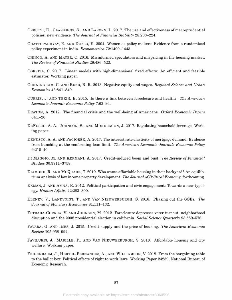
CERUTTI, E., CLAESSENS, S., AND LAEVEN, L. 2017. The use and effectiveness of macroprudentialpolicies: new evidence. The Journal of Financial Stability 28:203–224.

CHATTOPADHYAY, R. AND DUFLO, E. 2004. Women as policy makers: Evidence from a randomizedpolicy experiment in india. Econometrica 72:1409–1443.

CHINCO, A. AND MAYER, C. 2016. Misinformed speculators and mispricing in the housing market.The Review of Financial Studies 29:486–522.

CORREIA, S. 2017. Linear models with high-dimensional fixed effects: An efficient and feasibleestimator. Working paper.

CUNNINGHAM, C. AND REED, R. R. 2013. Negative equity and wages. Regional Science and UrbanEconomics 43:841–849.

CURRIE, J. AND TEKIN, E. 2015. Is there a link between foreclosure and health? The AmericanEconomic Journal: Economic Policy 7:63–94.

DEATON, A. 2012. The financial crisis and the well-being of Americans. Oxford Economic Papers64:1–26.

DEFUSCO, A. A., JOHNSON, S., AND MONDRAGON, J. 2017. Regulating household leverage. Work-ing paper.

DEFUSCO, A. A. AND PACIOREK, A. 2017. The interest rate elasticity of mortgage demand: Evidencefrom bunching at the conforming loan limit. The American Economic Journal: Economic Policy9:210–40.

DI MAGGIO, M. AND KERMANI, A. 2017. Credit-induced boom and bust. The Review of FinancialStudies 30:3711–3758.

DIAMOND, R. AND MCQUADE, T. 2019. Who wants affordable housing in their backyard? An equilib-rium analysis of low income property development. The Journal of Political Economy, forthcoming.

EKMAN, J. AND AMNÅ, E. 2012. Political participation and civic engagement: Towards a new typol-ogy. Human Affairs 22:283–300.

ELENEV, V., LANDVOIGT, T., AND VAN NIEUWERBURGH, S. 2016. Phasing out the GSEs. TheJournal of Monetary Economics 81:111–132.

ESTRADA-CORREA, V. AND JOHNSON, M. 2012. Foreclosure depresses voter turnout: neighborhooddisruption and the 2008 presidential election in california. Social Science Quarterly 93:559–576.

FAVARA, G. AND IMBS, J. 2015. Credit supply and the price of housing. The American EconomicReview 105:958–992.

FAVILUKIS, J., MABILLE, P., AND VAN NIEUWERBURGH, S. 2018. Affordable housing and citywelfare. Working paper.

FEIGENBAUM, J., HERTEL-FERNANDEZ, A., AND WILLIAMSON, V. 2018. From the bargaining tableto the ballot box: Political effects of right to work laws. Working Paper 24259, National Bureau ofEconomic Research.

27


FLOETOTTO, M., KIRKER, M., AND STROEBEL, J. 2016. Government intervention in the housingmarket: Who wins, who loses? The Journal of Monetary Economics 80:106–123.

FOOTE, C., GERARDI, K., GOETTE, L., AND WILLEN, P. 2010. Reducing foreclosures: No easyanswers. NBER Macroeconomics Annual 24:89–138.

FOOTE, C. L., GERARDI, K., AND WILLEN, P. S. 2008. Negative equity and foreclosure: Theory andevidence. The Journal of Urban Economics 64:234–245.

FRAME, W. S., FUSTER, A., TRACY, J., AND VICKERY, J. 2015. The rescue of Fannie Mae andFreddie Mac. The Journal of Economic Perspectives 29:25–52.

FUJIWARA, T. 2015. Voting technology, political responsiveness, and infant health: Evidence fromBrazil. Econometrica 83:423–464.

GANONG, P. AND NOEL, P. 2017. The effect of debt on default and consumption: Evidence fromhousing policy in the great recession. Working paper.

GETE, P. AND ZECCHETTO, F. 2017. Distributional implications of government guarantees in mort-gage markets. The Review of Financial Studies 31:1064–1097.

GIMPELSON, V. AND TREISMAN, D. 2018. Misperceiving inequality. Economics and Politics 30:27–54.

GLAESER, E. L. AND SHAPIRO, J. M. 2003. The benefits of the home mortgage interest deduction.Tax Policy and the Economy 17:37–82.

GUERRIERI, V., HARTLEY, D., AND HURST, E. 2013. Endogenous gentrification and housing pricedynamics. The Journal of Public Economics 100:45–60.

GUPTA, A. AND HANSMAN, C. 2019. Selection, leverage, and default in the mortgage market. Work-ing paper.

GYONGYOSI, G. AND VERNER, E. 2018. Financial crisis, creditor-debtor conflict, and political ex-tremism. Working paper.

HACAMO, I. 2016. Helping the middle-class: How interest rates affect the distribution of housingwealth. Working paper.

HALL, A. B. AND YODER, J. 2018. Does homeownership influence political behavior? Evidence fromadministrative data. Working paper.

HALL, A. B., YODER, J., AND KARANDIKAR, N. 2017. Economic distress and voting: Evidence fromthe subprime mortgage crisis. Working paper.

HILBER, C. A. AND TURNER, T. M. 2014. The mortgage interest deduction and its impact on home-ownership decisions. The Review of Economics and Statistics 96:618–637.

KEYS, B. J., POPE, D. G., AND POPE, J. C. 2016. Failure to refinance. The Journal of FinancialEconomics 122:482–499.

KING, G. 2013. A solution to the ecological inference problem: Reconstructing individual behaviorfrom aggregate data. Princeton University Press.

28


KRAMER, G. H. 1983. The ecological fallacy revisited: Aggregate-versus individual-level findings oneconomics and elections, and sociotropic voting. The American Political Science Review 77:92–111.

MELZER, B. T. 2017. Mortgage debt overhang: Reduced investment by homeowners at risk of default.The Journal of Finance 72:575–612.

MIAN, A., RAO, K., AND SUFI, A. 2013. Household balance sheets, consumption, and the economicslump. The Quarterly Journal of Economics 128:1687–1726.

MILLER, G. 2008. Women’s suffrage, political responsiveness, and child survival in American history.The Quarterly Journal of Economics 123:1287–1327.

ROBINSON, W. S. 2009. Ecological correlations and the behavior of individuals. The InternationalJournal of Epidemiology 38:337–341.

ROSENSTONE, S. J. 1982. Economic adversity and voter turnout. The American Journal of PoliticalScience pp. 25–46.

SCHMALZ, M. C., SRAER, D. A., AND THESMAR, D. 2017. Housing collateral and entrepreneurship.The Journal of Finance 72:99–132.

SODINI, P., VAN NIEUWERBURGH, S., VESTMAN, R., AND VON LILIENFELD-TOAL, U. 2016. Iden-tifying the benefits from home ownership: A swedish experiment. Working Paper 22882, NationalBureau of Economic Research.

SOLT, F. 2008. Economic inequality and democratic political engagement. The American Journal ofPolitical Science 52:48–60.

SOMMER, K. AND SULLIVAN, P. 2018. Implications of US tax policy for house prices, rents, andhomeownership. The American Economic Review 108:241–74.

VAN STRAELEN, H. 2018. From recession to revolution: Housing wealth and political polarization.Working paper.

YODER, J. 2019. How polling place changes reduce turnout: Evidence from administrative data inNorth Carolina. Working paper.

29


Figure 1: Percent Drop in NC Zip Code House Prices

This figure presents a choropleth map of zip codes in North Carolina (NC) as of November 2010, the month of the general election. Foreach zip code, I compute the change in the median house price over the previous 24 months using data from Zillow. The larger the declinein house prices, the more heavily shaded the zip code. Zip codes without home value data are left unshaded. 87% of the population of NClives in a shaded zip code.

30

Electronic copy available at: https://ssrn.com

/abstract=3068596

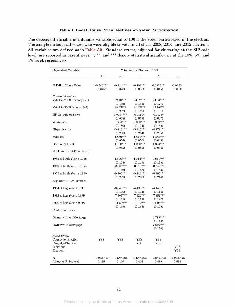
Table 1: Local House Price Declines on Voter Participation

The dependent variable is a dummy variable equal to 100 if the voter participated in the election.The sample includes all voters who were eligible to vote in all of the 2008, 2010, and 2012 elections.All variables are defined as in Table A2. Standard errors, adjusted for clustering at the ZIP codelevel, are reported in parentheses. *, **, and *** denote statistical significance at the 10%, 5%, and1% level, respectively.

Dependent Variable: Voted in the Election (=100)

(1) (2) (3) (4) (5)

% Fall in Home Value -0.240*** -0.124*** -0.102*** -0.0835*** -0.0623*(0.045) (0.020) (0.018) (0.015) (0.033)

Control VariablesVoted in 2008 Primary (=1) 22.10*** 23.82*** 23.38***

(0.155) (0.135) (0.127)Voted in 2008 General (=1) 35.63*** 34.67*** 33.70***

(0.202) (0.189) (0.191)HP Growth ’04 to ’08 0.0204*** 0.0129* 0.0128*

(0.008) (0.007) (0.007)White (=1) 6.824*** 3.300*** 2.389***

(0.180) (0.174) (0.159)Hispanic (=1) -3.418*** -3.945*** -4.179***

(0.200) (0.204) (0.205)Male (=1) 1.866*** 1.521*** 1.335***

(0.055) (0.050) (0.049)Born in NC (=1) 1.168*** 1.220*** 1.323***

(0.085) (0.085) (0.084)Birth Year ≤ 1942 (omitted)

1943 ≤ Birth Year ≤ 1958 1.506*** 1.314*** 0.851***(0.128) (0.119) (0.123)

1959 ≤ Birth Year ≤ 1974 -2.606*** -3.019*** -3.546***(0.166) (0.158) (0.163)

1975 ≤ Birth Year ≤ 1990 -9.166*** -9.246*** -8.980***(0.279) (0.256) (0.244)

Reg Year ≤ 1983 (omitted)

1984 ≤ Reg Year ≤ 1991 -3.846*** -4.499*** -4.443***(0.116) (0.114) (0.114)

1992 ≤ Reg Year ≤ 1999 -7.306*** -7.922*** -7.882***(0.151) (0.151) (0.147)

2000 ≤ Reg Year ≤ 2008 -11.80*** -12.17*** -11.96***(0.169) (0.168) (0.158)

Renter (omitted)

Owner without Mortgage 4.715***(0.146)

Owner with Mortgage 7.546***(0.150)

Fixed EffectsCounty-by-Election YES YES YES YESParty-by-Election YES YESIndividual YESElection YES

N 12,925,463 12,686,292 12,686,292 12,686,292 12,923,456Adjusted R-Squared 0.165 0.409 0.416 0.419 0.534

31


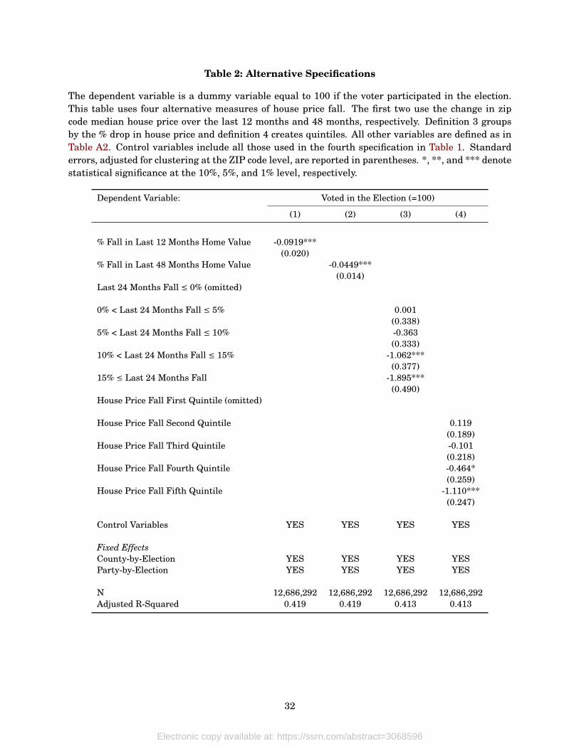
Table 2: Alternative Specifications

The dependent variable is a dummy variable equal to 100 if the voter participated in the election.This table uses four alternative measures of house price fall. The first two use the change in zipcode median house price over the last 12 months and 48 months, respectively. Definition 3 groupsby the % drop in house price and definition 4 creates quintiles. All other variables are defined as inTable A2. Control variables include all those used in the fourth specification in Table 1. Standarderrors, adjusted for clustering at the ZIP code level, are reported in parentheses. *, **, and *** denotestatistical significance at the 10%, 5%, and 1% level, respectively.


(1) (2) (3) (4)

% Fall in Last 12 Months Home Value -0.0919***(0.020)

% Fall in Last 48 Months Home Value -0.0449***(0.014)

Last 24 Months Fall ≤ 0% (omitted)

0% < Last 24 Months Fall ≤ 5% 0.001(0.338)

5% < Last 24 Months Fall ≤ 10% -0.363(0.333)

10% < Last 24 Months Fall ≤ 15% -1.062***(0.377)

15% ≤ Last 24 Months Fall -1.895***(0.490)

House Price Fall First Quintile (omitted)

House Price Fall Second Quintile 0.119(0.189)

House Price Fall Third Quintile -0.101(0.218)

House Price Fall Fourth Quintile -0.464*(0.259)

House Price Fall Fifth Quintile -1.110***(0.247)

Control Variables YES YES YES YES

Fixed EffectsCounty-by-Election YES YES YES YESParty-by-Election YES YES YES YES

N 12,686,292 12,686,292 12,686,292 12,686,292Adjusted R-Squared 0.419 0.419 0.413 0.413

32


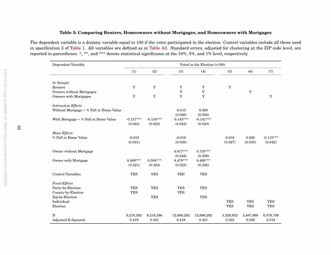
Table 3: Comparing Renters, Homeowners without Mortgages, and Homeowners with Mortgages

The dependent variable is a dummy variable equal to 100 if the voter participated in the election. Control variables include all those usedin specification 3 of Table 1. All variables are defined as in Table A2. Standard errors, adjusted for clustering at the ZIP code level, arereported in parentheses. *, **, and *** denote statistical significance at the 10%, 5%, and 1% level, respectively.

Dependent Variable Voted in the Election (=100)

(1) (2) (3) (4) (5) (6) (7)

In SampleRenters Y Y Y Y YOwners without Mortgages Y Y YOwners with Mortgages Y Y Y Y Y

Interaction EffectsWithout Mortgage × % Fall in Home Value -0.013 0.000

(0.026) (0.026)With Mortgage × % Fall in Home Value -0.137*** -0.134*** -0.143*** -0.141***

(0.042) (0.042) (0.043) (0.043)

Main Effects% Fall in Home Value -0.018 -0.018 0.018 0.026 -0.110***

(0.031) (0.030) (0.027) (0.035) (0.042)

Owner without Mortgage 4.817*** 4.733***(0.242) (0.239)

Owner with Mortgage 8.489*** 8.504*** 8.479*** 8.498***(0.321) (0.324) (0.323) (0.326)


Fixed EffectsParty-by-Election YES YES YES YESCounty-by-Election YES YESZip-by-Election YES YESIndividual YES YES YESElection YES YES YES

N 9,218,382 9,218,386 12,686,292 12,686,292 3,329,932 3,487,968 6,079,709Adjusted R-Squared 0.419 0.421 0.419 0.421 0.522 0.539 0.518

33


/abstract=3068596

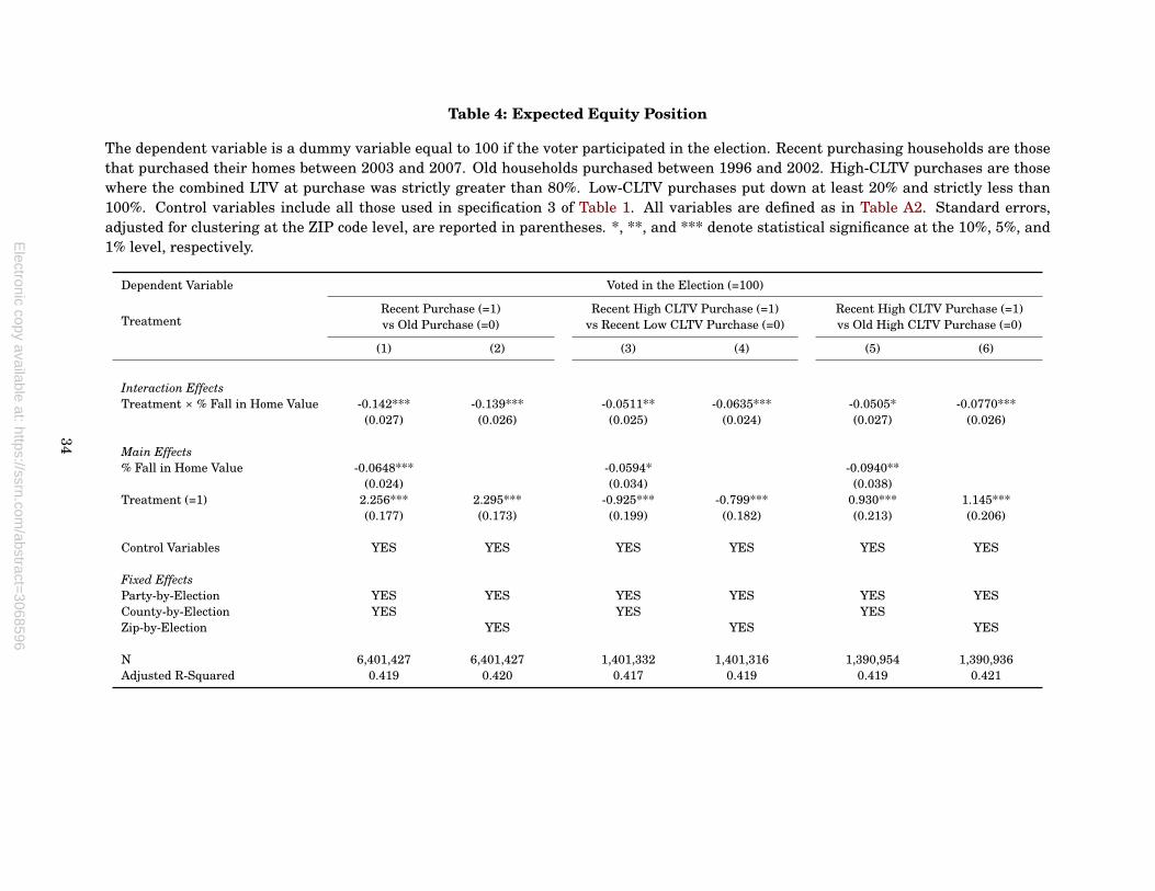
Table 4: Expected Equity Position

The dependent variable is a dummy variable equal to 100 if the voter participated in the election. Recent purchasing households are thosethat purchased their homes between 2003 and 2007. Old households purchased between 1996 and 2002. High-CLTV purchases are thosewhere the combined LTV at purchase was strictly greater than 80%. Low-CLTV purchases put down at least 20% and strictly less than100%. Control variables include all those used in specification 3 of Table 1. All variables are defined as in Table A2. Standard errors,adjusted for clustering at the ZIP code level, are reported in parentheses. *, **, and *** denote statistical significance at the 10%, 5%, and1% level, respectively.


TreatmentRecent Purchase (=1) Recent High CLTV Purchase (=1) Recent High CLTV Purchase (=1)vs Old Purchase (=0) vs Recent Low CLTV Purchase (=0) vs Old High CLTV Purchase (=0)

(1) (2) (3) (4) (5) (6)

Interaction EffectsTreatment × % Fall in Home Value -0.142*** -0.139*** -0.0511** -0.0635*** -0.0505* -0.0770***

(0.027) (0.026) (0.025) (0.024) (0.027) (0.026)

Main Effects% Fall in Home Value -0.0648*** -0.0594* -0.0940**

(0.024) (0.034) (0.038)Treatment (=1) 2.256*** 2.295*** -0.925*** -0.799*** 0.930*** 1.145***

(0.177) (0.173) (0.199) (0.182) (0.213) (0.206)

Control Variables YES YES YES YES YES YES

Fixed EffectsParty-by-Election YES YES YES YES YES YESCounty-by-Election YES YES YESZip-by-Election YES YES YES

N 6,401,427 6,401,427 1,401,332 1,401,316 1,390,954 1,390,936Adjusted R-Squared 0.419 0.420 0.417 0.419 0.419 0.421

34


/abstract=3068596

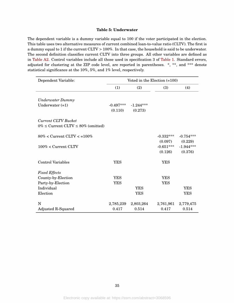
Table 5: Underwater

The dependent variable is a dummy variable equal to 100 if the voter participated in the election.This table uses two alternative measures of current combined loan-to-value ratio (CLTV). The first isa dummy equal to 1 if the current CLTV > 100%. In that case, the household is said to be underwater.The second definition classifies current CLTV into three groups. All other variables are defined asin Table A2. Control variables include all those used in specification 3 of Table 1. Standard errors,adjusted for clustering at the ZIP code level, are reported in parentheses. *, **, and *** denotestatistical significance at the 10%, 5%, and 1% level, respectively.


(1) (2) (3) (4)

Underwater DummyUnderwater (=1) -0.497*** -1.244***

(0.110) (0.273)

Current CLTV Bucket0% ≤ Current CLTV ≤ 80% (omitted)

80% < Current CLTV < =100% -0.332*** -0.754***(0.097) (0.229)

100% < Current CLTV -0.651*** -1.944***(0.126) (0.376)

Control Variables YES YES

Fixed EffectsCounty-by-Election YES YESParty-by-Election YES YESIndividual YES YESElection YES YES


35


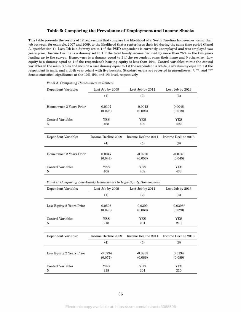
Table 6: Comparing the Prevalence of Employment and Income Shocks

This table presents the results of 12 regressions that compare the likelihood of a North Carolina homeowner losing theirjob between, for example, 2007 and 2009, to the likelihood that a renter loses their job during the same time period (PanelA, specification 1). Lost Job is a dummy set to 1 if the PSID respondent is currently unemployed and was employed twoyears prior. Income Decline is a dummy set to 1 if the total family income declined by more than 25% in the two yearsleading up to the survey. Homeowner is a dummy equal to 1 if the respondent owns their home and 0 otherwise. Lowequity is a dummy equal to 1 if the respondent’s housing equity is less than 10%. Control variables mimic the controlvariables in the main tables and include a race dummy equal to 1 if the respondent is white, a sex dummy equal to 1 if therespondent is male, and a birth year cohort with five buckets. Standard errors are reported in parentheses. *, **, and ***denote statistical significance at the 10%, 5%, and 1% level, respectively.

Panel A: Comparing Homeowners to Renters

Dependent Variable: Lost Job by 2009 Lost Job by 2011 Lost Job by 2013

(1) (2) (3)

Homeowner 2 Years Prior 0.0107 -0.0012 0.0048(0.026) (0.023) (0.018)

Control Variables YES YES YESN 468 492 492

Dependent Variable: Income Decline 2009 Income Decline 2011 Income Decline 2013

(4) (5) (6)

Homeowner 2 Years Prior 0.0047 -0.0220 -0.0740(0.044) (0.053) (0.045)


Panel B: Comparing Low-Equity Homeowners to High-Equity Homeowners


(1) (2) (3)

Low Equity 2 Years Prior 0.0505 0.0399 -0.0395*(0.078) (0.060) (0.020)



(4) (5) (6)

Low Equity 2 Years Prior -0.0794 -0.0985 0.0194(0.077) (0.086) (0.089)


36


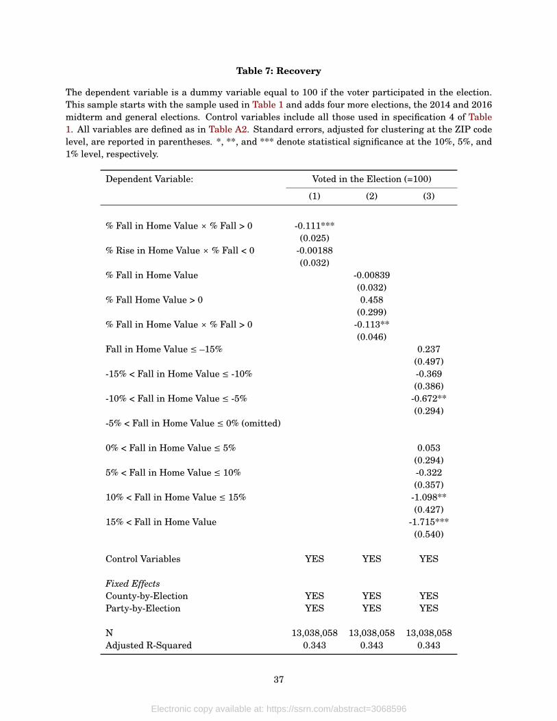
Table 7: Recovery

The dependent variable is a dummy variable equal to 100 if the voter participated in the election.This sample starts with the sample used in Table 1 and adds four more elections, the 2014 and 2016midterm and general elections. Control variables include all those used in specification 4 of Table1. All variables are defined as in Table A2. Standard errors, adjusted for clustering at the ZIP codelevel, are reported in parentheses. *, **, and *** denote statistical significance at the 10%, 5%, and1% level, respectively.


(1) (2) (3)

% Fall in Home Value × % Fall > 0 -0.111***(0.025)

% Rise in Home Value × % Fall < 0 -0.00188(0.032)

% Fall in Home Value -0.00839(0.032)

% Fall Home Value > 0 0.458(0.299)

% Fall in Home Value × % Fall > 0 -0.113**(0.046)

Fall in Home Value ≤ –15% 0.237(0.497)

-15% < Fall in Home Value ≤ -10% -0.369(0.386)

-10% < Fall in Home Value ≤ -5% -0.672**(0.294)

-5% < Fall in Home Value ≤ 0% (omitted)

0% < Fall in Home Value ≤ 5% 0.053(0.294)

5% < Fall in Home Value ≤ 10% -0.322(0.357)

10% < Fall in Home Value ≤ 15% -1.098**(0.427)

15% < Fall in Home Value -1.715***(0.540)

Control Variables YES YES YES

Fixed EffectsCounty-by-Election YES YES YESParty-by-Election YES YES YES

N 13,038,058 13,038,058 13,038,058Adjusted R-Squared 0.343 0.343 0.343

37


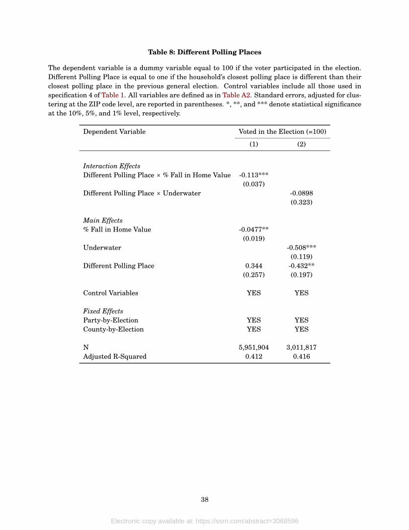
Table 8: Different Polling Places

The dependent variable is a dummy variable equal to 100 if the voter participated in the election.Different Polling Place is equal to one if the household’s closest polling place is different than theirclosest polling place in the previous general election. Control variables include all those used inspecification 4 of Table 1. All variables are defined as in Table A2. Standard errors, adjusted for clus-tering at the ZIP code level, are reported in parentheses. *, **, and *** denote statistical significanceat the 10%, 5%, and 1% level, respectively.


(1) (2)

Interaction EffectsDifferent Polling Place × % Fall in Home Value -0.113***

(0.037)Different Polling Place × Underwater -0.0898

(0.323)

Main Effects% Fall in Home Value -0.0477**

(0.019)Underwater -0.508***

(0.119)Different Polling Place 0.344 -0.432**

(0.257) (0.197)


Fixed EffectsParty-by-Election YES YESCounty-by-Election YES YES

N 5,951,904 3,011,817Adjusted R-Squared 0.412 0.416

38


ONLINE APPENDIX

Does Household Finance Affect the Political Process? Evidence fromVoter Turnout During a Housing Crisis

February, 2020

This is the online appendix for “Does Household Finance Affect the Political Process? Evidence from

Voter Turnout During a Housing Crisis.”

• Appendix A contains supplemental tables.

• Appendix B contains more detail on the data, especially the merging algorithm between the

voter rolls data and the deeds data, the limitations of this data, and the creation of the CLTV

variable.

• Appendix C presents other implied aggregate effects of house price declines on voter turnout.

39


A Supplemental Tables

40


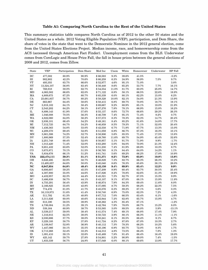
Table A1: Comparing North Carolina to the Rest of the United States

This summary statistics table compares North Carolina as of 2012 to the other 50 states and theUnited States as a whole. 2012 Voting Eligible Population (VEP), participation, and Dem Share, theshare of votes in the state that went to the Democratic Nominee in the 2012 general election, comefrom the United States Elections Project. Median income, race, and homeownership come from theACS (accessed through American Fact Finder). Unemployment comes from the BLS. Underwatercomes from CoreLogic and House Price Fall, the fall in house prices between the general elections of2008 and 2012, comes from Zillow.

State VEP Participation Dem Share Med Inc Unem White Homeowner Underwater HP Fall

DC 477,582 60.9% 90.9% $ 66,583 9.3% 39.6% 41.5% -3.2%HI 982,902 42.2% 70.6% $ 66,259 6.3% 24.9% 56.9% 7.5% 9.7%VT 493,355 63.7% 66.6% $ 52,977 4.6% 95.1% 71.0% 3.8%NY 13,324,107 56.8% 63.4% $ 56,448 8.6% 65.2% 53.7% 7.7% 16.1%RI 768,918 59.0% 62.7% $ 54,554 11.0% 81.7% 60.0% 25.8% 14.7%MD 4,063,582 66.6% 62.0% $ 71,122 6.8% 58.1% 66.5% 22.6% 18.9%MA 4,809,675 67.2% 60.7% $ 65,339 6.0% 80.1% 62.2% 15.0% 6.2%CA 23,681,837 56.7% 60.2% $ 58,328 10.8% 62.1% 54.0% 21.3% 13.9%DE 663,967 64.4% 58.6% $ 58,415 6.8% 69.7% 70.8% 18.7% 19.1%NJ 5,918,182 64.1% 58.4% $ 69,667 9.2% 68.9% 65.1% 19.0% 21.9%CT 2,543,202 64.2% 58.1% $ 67,276 7.8% 78.1% 66.9% 15.8% 16.2%IL 8,899,143 61.9% 57.6% $ 55,137 8.6% 72.7% 66.6% 29.2% 26.3%ME 1,046,008 70.5% 56.3% $ 46,709 7.4% 95.1% 71.4% 9.2% 0.7%WA 4,822,060 64.8% 56.2% $ 57,573 8.3% 78.3% 62.3% 14.7% 20.4%OR 2,836,101 66.4% 54.2% $ 49,161 8.4% 85.2% 61.6% 14.8% 17.7%MI 7,312,725 64.7% 54.2% $ 46,859 8.5% 79.3% 71.1% 32.0% 20.4%NM 1,436,363 54.8% 53.0% $ 42,558 6.7% 71.9% 67.7% 13.3% 15.0%WI 4,209,370 69.4% 52.8% $ 51,059 6.8% 86.7% 67.3% 16.3% 10.1%MN 3,861,598 74.2% 52.7% $ 58,906 5.6% 85.5% 71.4% 17.5% 13.8%NV 1,800,969 57.3% 52.4% $ 49,760 11.6% 69.7% 54.9% 45.4% 32.6%IA 2,251,748 68.4% 52.0% $ 50,957 5.1% 91.7% 71.9% 9.9% -1.7%NH 1,013,420 71.4% 52.0% $ 63,280 5.0% 94.0% 70.9% 21.3% 12.4%PA 9,651,432 63.6% 52.0% $ 51,230 7.4% 81.9% 68.9% 10.3% 8.7%CO 3,675,871 70.1% 51.5% $ 56,765 8.1% 84.4% 64.0% 14.2% 1.1%VA 5,834,676 66.1% 51.2% $ 61,741 5.6% 69.2% 66.2% 17.0% 10.9%USA 222,474,111 59.3% 51.1% $ 51,371 8.2% 73.9% 63.9% 19.8% 13.8%OH 8,649,495 62.9% 50.7% $ 46,829 7.3% 82.7% 66.3% 26.3% 10.2%FL 13,495,057 64.6% 50.0% $ 45,040 8.6% 76.3% 65.6% 38.1% 28.0%NC 6,947,954 64.8% 48.4% $ 45,150 9.4% 69.9% 65.4% 12.2% 9.9%GA 6,606,607 59.2% 45.5% $ 47,209 8.9% 60.4% 63.7% 30.5% 25.4%AZ 4,387,900 55.0% 44.6% $ 47,826 8.2% 78.8% 62.6% 31.3% 19.9%MO 4,432,957 62.3% 44.4% $ 45,321 7.3% 82.7% 67.5% 15.3% 9.9%SC 3,486,838 56.7% 44.1% $ 43,107 9.1% 67.0% 68.1% 15.9% 11.9%IN 4,755,291 56.4% 43.9% $ 46,974 7.9% 84.3% 69.4% 11.6% 8.0%MS 2,166,825 55.6% 43.8% $ 37,095 8.7% 59.3% 68.2% 22.3% 7.5%MT 774,476 61.8% 41.7% $ 45,076 6.3% 89.2% 67.1% 5.6% 0.3%TX 16,119,973 51.6% 41.4% $ 50,740 6.9% 75.0% 62.3% 7.2% 4.3%AK 511,792 61.3% 40.8% $ 67,712 7.0% 66.5% 63.4% 6.1% -1.6%LA 3,311,626 60.0% 40.6% $ 42,944 7.2% 62.8% 65.7% 15.9% 4.7%SD 613,190 58.5% 39.9% $ 48,362 4.3% 85.4% 67.1% -1.2%TN 4,736,084 51.2% 39.1% $ 42,764 7.9% 78.0% 66.7% 15.2% 8.0%ND 539,164 60.9% 38.7% $ 53,585 3.0% 89.5% 65.0% 5.9% -13.1%AL 3,539,217 59.0% 38.4% $ 41,574 7.4% 69.1% 68.8% 17.4% 7.9%NE 1,316,915 62.5% 38.0% $ 50,723 3.9% 88.1% 66.3% 11.1% -1.1%KS 2,030,686 57.7% 38.0% $ 50,241 6.1% 85.5% 66.4% 9.1% 6.7%KY 3,229,185 58.7% 37.8% $ 41,724 8.2% 87.8% 67.0% 10.3% 2.7%AR 2,109,847 52.8% 36.9% $ 40,112 7.3% 78.3% 66.2% 10.2% 5.6%WV 1,447,066 50.1% 35.5% $ 40,196 6.9% 93.7% 72.0% 9.3% 1.7%OK 2,713,268 52.4% 33.2% $ 44,312 4.8% 73.5% 66.4% 7.8% 1.3%ID 1,091,410 59.1% 32.6% $ 45,489 7.8% 91.4% 68.4% 16.4% 19.0%WY 425,142 59.7% 27.8% $ 54,901 5.2% 90.9% 69.0% 7.4% -1.5%UT 1,833,339 56.7% 24.8% $ 57,049 6.0% 88.1% 69.6% 13.9% 17.7%

41


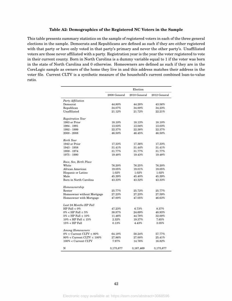
Table A2: Demographics of the Registered NC Voters in the Sample

This table presents summary statistics on the sample of registered voters in each of the three generalelections in the sample. Democrats and Republicans are defined as such if they are either registeredwith that party or have only voted in that party’s primary and never the other party’s. Unaffiliatedvoters are those never affiliated with a party. Registration year is the year the voter registered to votein their current county. Born in North Carolina is a dummy variable equal to 1 if the voter was bornin the state of North Carolina and 0 otherwise. Homeowners are defined as such if they are in theCoreLogic sample as owners of the home they live in and this address matches their address in thevoter file. Current CLTV is a synthetic measure of the household’s current combined loan-to-valueratio.

Election

2008 General 2010 General 2012 General

Party AffiliationDemocrat 44.80% 44.28% 43.56%Republican 34.07% 34.00% 34.23%Unaffiliated 21.12% 21.72% 22.21%

Regsitration Year1983 or Prior 18.10% 18.13% 18.10%1984 - 1991 13.03% 13.04% 13.03%1992 - 1999 22.37% 22.38% 22.37%2000 - 2008 46.50% 46.45% 46.50%

Birth Year1942 or Prior 17.33% 17.36% 17.33%1943 - 1958 31.41% 31.44% 31.41%1959 - 1974 31.77% 31.77% 31.77%1975 - 1990 19.48% 19.43% 19.48%

Race, Sex, Birth PlaceWhite 76.20% 76.25% 76.20%African American 19.05% 19.01% 19.05%Hispanic or Latino 1.02% 1.02% 1.02%Male 45.39% 45.40% 45.39%Born in North Carolina 43.33% 43.32% 43.33%

HomeownershipRenter 25.77% 25.72% 25.77%Homeowner without Mortgage 27.23% 27.23% 27.59%Homeowner with Mortgage 47.00% 47.05% 46.63%

Last 24 Months HP FallHP Fall ≤ 0% 47.23% 6.73% 8.37%0% < HP Fall ≤ 5% 38.87% 24.69% 48.93%5% < HP Fall ≤ 10% 11.46% 44.78% 32.00%10% < HP Fall ≤ 15% 2.32% 19.37% 7.65%15% < HP Fall 0.13% 4.43% 3.05%

Among Homeowners0% ≤ Current CLTV ≤ 80% 64.18% 58.24% 57.77%80% < Current CLTV ≤ 100% 27.86% 27.00% 25.41%100% < Current CLTV 7.97% 14.76% 16.82%

N 3,175,677 3,167,469 3,175,677

42


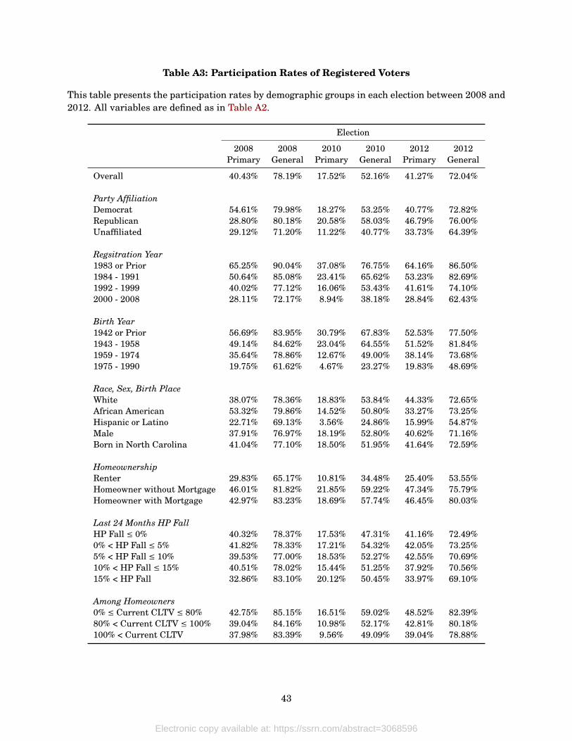
Table A3: Participation Rates of Registered Voters

This table presents the participation rates by demographic groups in each election between 2008 and2012. All variables are defined as in Table A2.

Election

2008 2008 2010 2010 2012 2012Primary General Primary General Primary General

Overall 40.43% 78.19% 17.52% 52.16% 41.27% 72.04%

Party AffiliationDemocrat 54.61% 79.98% 18.27% 53.25% 40.77% 72.82%Republican 28.80% 80.18% 20.58% 58.03% 46.79% 76.00%Unaffiliated 29.12% 71.20% 11.22% 40.77% 33.73% 64.39%

Regsitration Year1983 or Prior 65.25% 90.04% 37.08% 76.75% 64.16% 86.50%1984 - 1991 50.64% 85.08% 23.41% 65.62% 53.23% 82.69%1992 - 1999 40.02% 77.12% 16.06% 53.43% 41.61% 74.10%2000 - 2008 28.11% 72.17% 8.94% 38.18% 28.84% 62.43%

Birth Year1942 or Prior 56.69% 83.95% 30.79% 67.83% 52.53% 77.50%1943 - 1958 49.14% 84.62% 23.04% 64.55% 51.52% 81.84%1959 - 1974 35.64% 78.86% 12.67% 49.00% 38.14% 73.68%1975 - 1990 19.75% 61.62% 4.67% 23.27% 19.83% 48.69%

Race, Sex, Birth PlaceWhite 38.07% 78.36% 18.83% 53.84% 44.33% 72.65%African American 53.32% 79.86% 14.52% 50.80% 33.27% 73.25%Hispanic or Latino 22.71% 69.13% 3.56% 24.86% 15.99% 54.87%Male 37.91% 76.97% 18.19% 52.80% 40.62% 71.16%Born in North Carolina 41.04% 77.10% 18.50% 51.95% 41.64% 72.59%

HomeownershipRenter 29.83% 65.17% 10.81% 34.48% 25.40% 53.55%Homeowner without Mortgage 46.01% 81.82% 21.85% 59.22% 47.34% 75.79%Homeowner with Mortgage 42.97% 83.23% 18.69% 57.74% 46.45% 80.03%

Last 24 Months HP FallHP Fall ≤ 0% 40.32% 78.37% 17.53% 47.31% 41.16% 72.49%0% < HP Fall ≤ 5% 41.82% 78.33% 17.21% 54.32% 42.05% 73.25%5% < HP Fall ≤ 10% 39.53% 77.00% 18.53% 52.27% 42.55% 70.69%10% < HP Fall ≤ 15% 40.51% 78.02% 15.44% 51.25% 37.92% 70.56%15% < HP Fall 32.86% 83.10% 20.12% 50.45% 33.97% 69.10%

Among Homeowners0% ≤ Current CLTV ≤ 80% 42.75% 85.15% 16.51% 59.02% 48.52% 82.39%80% < Current CLTV ≤ 100% 39.04% 84.16% 10.98% 52.17% 42.81% 80.18%100% < Current CLTV 37.98% 83.39% 9.56% 49.09% 39.04% 78.88%

43


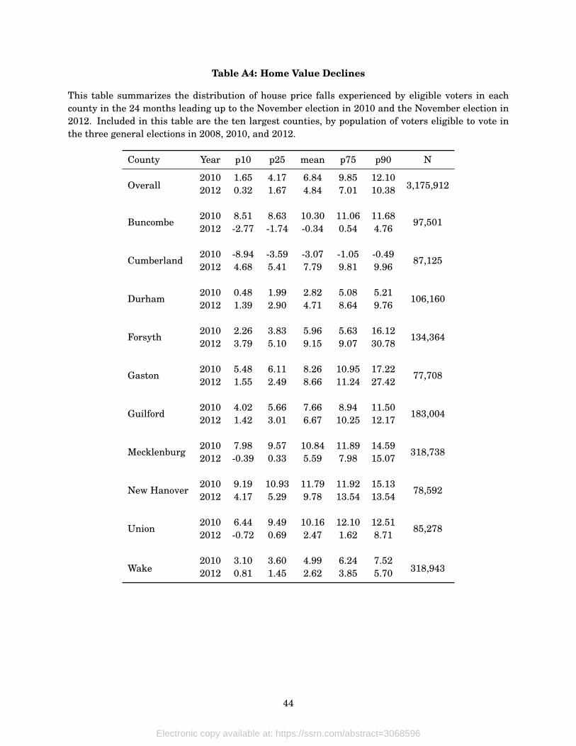
Table A4: Home Value Declines

This table summarizes the distribution of house price falls experienced by eligible voters in eachcounty in the 24 months leading up to the November election in 2010 and the November election in2012. Included in this table are the ten largest counties, by population of voters eligible to vote inthe three general elections in 2008, 2010, and 2012.

County Year p10 p25 mean p75 p90 N

Overall2010 1.65 4.17 6.84 9.85 12.10

3,175,9122012 0.32 1.67 4.84 7.01 10.38

Buncombe2010 8.51 8.63 10.30 11.06 11.68

97,5012012 -2.77 -1.74 -0.34 0.54 4.76

Cumberland2010 -8.94 -3.59 -3.07 -1.05 -0.49

87,1252012 4.68 5.41 7.79 9.81 9.96

Durham2010 0.48 1.99 2.82 5.08 5.21

106,1602012 1.39 2.90 4.71 8.64 9.76

Forsyth2010 2.26 3.83 5.96 5.63 16.12

134,3642012 3.79 5.10 9.15 9.07 30.78

Gaston2010 5.48 6.11 8.26 10.95 17.22

77,7082012 1.55 2.49 8.66 11.24 27.42

Guilford2010 4.02 5.66 7.66 8.94 11.50

183,0042012 1.42 3.01 6.67 10.25 12.17

Mecklenburg2010 7.98 9.57 10.84 11.89 14.59

318,7382012 -0.39 0.33 5.59 7.98 15.07

New Hanover2010 9.19 10.93 11.79 11.92 15.13

78,5922012 4.17 5.29 9.78 13.54 13.54

Union2010 6.44 9.49 10.16 12.10 12.51

85,2782012 -0.72 0.69 2.47 1.62 8.71

Wake2010 3.10 3.60 4.99 6.24 7.52

318,9432012 0.81 1.45 2.62 3.85 5.70

44


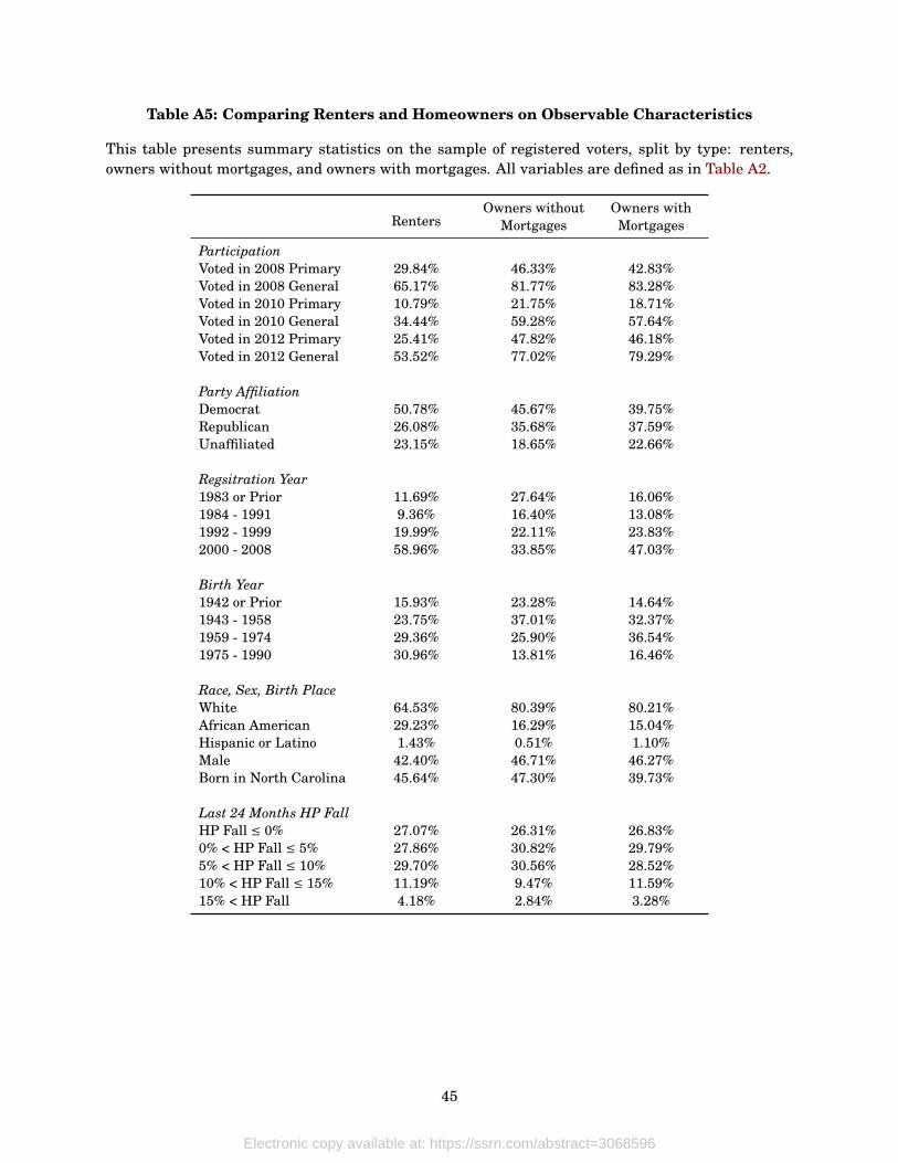
Table A5: Comparing Renters and Homeowners on Observable Characteristics

This table presents summary statistics on the sample of registered voters, split by type: renters,owners without mortgages, and owners with mortgages. All variables are defined as in Table A2.

RentersOwners without Owners with

Mortgages Mortgages

ParticipationVoted in 2008 Primary 29.84% 46.33% 42.83%Voted in 2008 General 65.17% 81.77% 83.28%Voted in 2010 Primary 10.79% 21.75% 18.71%Voted in 2010 General 34.44% 59.28% 57.64%Voted in 2012 Primary 25.41% 47.82% 46.18%Voted in 2012 General 53.52% 77.02% 79.29%


Regsitration Year1983 or Prior 11.69% 27.64% 16.06%1984 - 1991 9.36% 16.40% 13.08%1992 - 1999 19.99% 22.11% 23.83%2000 - 2008 58.96% 33.85% 47.03%

Birth Year1942 or Prior 15.93% 23.28% 14.64%1943 - 1958 23.75% 37.01% 32.37%1959 - 1974 29.36% 25.90% 36.54%1975 - 1990 30.96% 13.81% 16.46%



45


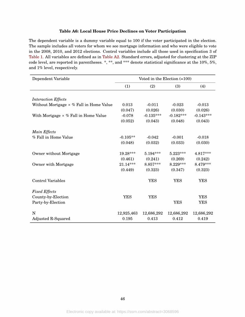
Table A6: Local House Price Declines on Voter Participation

The dependent variable is a dummy variable equal to 100 if the voter participated in the election.The sample includes all voters for whom we see mortgage information and who were eligible to votein the 2008, 2010, and 2012 elections. Control variables include all those used in specification 3 ofTable 1. All variables are defined as in Table A2. Standard errors, adjusted for clustering at the ZIPcode level, are reported in parentheses. *, **, and *** denote statistical significance at the 10%, 5%,and 1% level, respectively.


(1) (2) (3) (4)

Interaction EffectsWithout Mortgage × % Fall in Home Value 0.013 -0.011 -0.023 -0.013

(0.047) (0.026) (0.030) (0.026)With Mortgage × % Fall in Home Value -0.078 -0.135*** -0.182*** -0.143***

(0.052) (0.043) (0.048) (0.043)

Main Effects% Fall in Home Value -0.105** -0.042 -0.001 -0.018

(0.048) (0.032) (0.033) (0.030)

Owner without Mortgage 19.28*** 5.194*** 5.223*** 4.817***(0.461) (0.241) (0.269) (0.242)



Fixed EffectsCounty-by-Election YES YES YESParty-by-Election YES YES


46


Table A7: ZIP Code Income

The dependent variable is a dummy variable equal to 100 if the voter participated in the election.The % change in ZIP code income comes from the IRS and is described in detail in the text. Controlvariables include all those used in Table 1. All variables are defined as in Table A2. Standard errors,adjusted for clustering at the ZIP code level, are reported in parentheses. *, **, and *** denotestatistical significance at the 10%, 5%, and 1% level, respectively.


(1) (2) (3)

% Fall in Home Value -0.0674*** -0.137*** -0.114***(0.019) (0.030) (0.025)

% Change Zip Income 0.00026(0.000)

% Change Zip Income > 0 -1.276***(0.318)

% Change Zip Income > 0 × % Fall in Home Value 0.0906**(0.035)

% Change Zip Income > Median -0.714***(0.255)

% Change Zip Income > Median × % Fall in Home Value 0.0993***(0.033)


Fixed EffectsParty-by-Election YES YES YESCounty-by-Election YES YES YES

N 5,951,440 5,951,440 5,951,440Adjusted R-Squared 0.412 0.412 0.412

47


Table A8: Heterogeneity of Effects Across County Unemployment Levels

This table estimates specification (3) from Table 3 on four subsamples, split by county-level un-employment rates. Standard errors, adjusted for clustering at the ZIP code level, are reported inparentheses. *, **, and *** denote statistical significance at the 10%, 5%, and 1% level, respectively.


(1) (2) (3) (4)

SampleCounty Unemployment ≤ 9.7% Y9.7% < County Unemployment ≤ 10.7% Y10.7% < County Unemployment ≤ 12.3% Y12.3% < County Unemployment Y

Interaction EffectsWithout Mortgage × % Fall in Home Value -0.001 -0.031 0.091 0.000

(0.067) (0.046) (0.080) (0.053)With Mortgage × % Fall in Home Value -0.081 -0.205** -0.223* -0.077

(0.079) (0.085) (0.123) (0.075)

Main Effects% Fall in Home Value -0.015 -0.0868** 0.135 0.044

(0.081) (0.044) (0.105) (0.072)




Fixed EffectsParty-by-Election YES YES YES YES


48


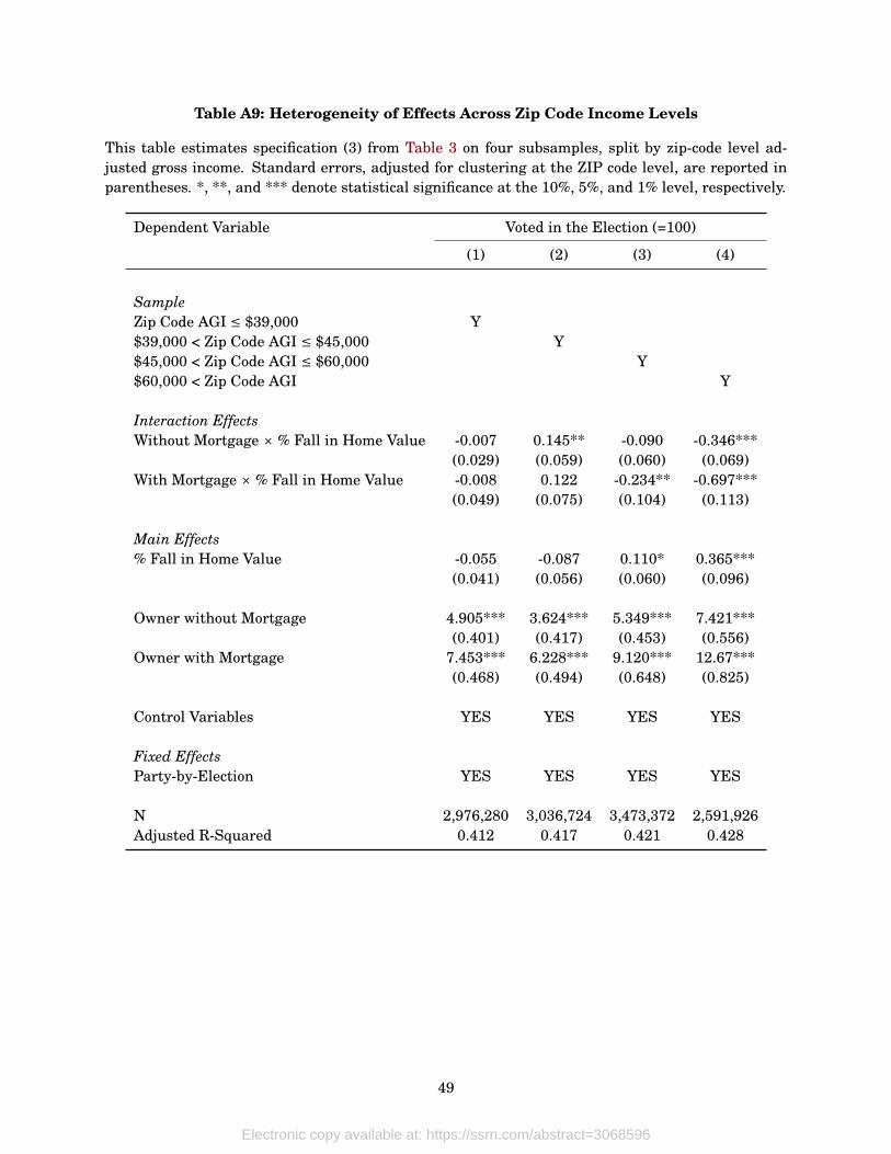
Table A9: Heterogeneity of Effects Across Zip Code Income Levels

This table estimates specification (3) from Table 3 on four subsamples, split by zip-code level ad-justed gross income. Standard errors, adjusted for clustering at the ZIP code level, are reported inparentheses. *, **, and *** denote statistical significance at the 10%, 5%, and 1% level, respectively.


(1) (2) (3) (4)

SampleZip Code AGI ≤ $39,000 Y$39,000 < Zip Code AGI ≤ $45,000 Y$45,000 < Zip Code AGI ≤ $60,000 Y$60,000 < Zip Code AGI Y

Interaction EffectsWithout Mortgage × % Fall in Home Value -0.007 0.145** -0.090 -0.346***

(0.029) (0.059) (0.060) (0.069)With Mortgage × % Fall in Home Value -0.008 0.122 -0.234** -0.697***

(0.049) (0.075) (0.104) (0.113)

Main Effects% Fall in Home Value -0.055 -0.087 0.110* 0.365***

(0.041) (0.056) (0.060) (0.096)




Fixed EffectsParty-by-Election YES YES YES YES


49


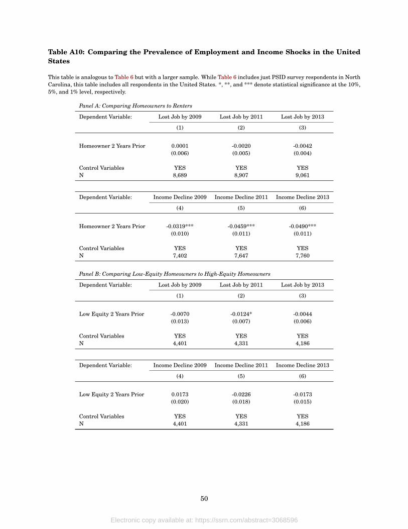
Table A10: Comparing the Prevalence of Employment and Income Shocks in the UnitedStates

This table is analogous to Table 6 but with a larger sample. While Table 6 includes just PSID survey respondents in NorthCarolina, this table includes all respondents in the United States. *, **, and *** denote statistical significance at the 10%,5%, and 1% level, respectively.

Panel A: Comparing Homeowners to Renters


(1) (2) (3)

Homeowner 2 Years Prior 0.0001 -0.0020 -0.0042(0.006) (0.005) (0.004)

Control Variables YES YES YESN 8,689 8,907 9,061


(4) (5) (6)

Homeowner 2 Years Prior -0.0319*** -0.0459*** -0.0490***(0.010) (0.011) (0.011)


Panel B: Comparing Low-Equity Homeowners to High-Equity Homeowners


(1) (2) (3)

Low Equity 2 Years Prior -0.0070 -0.0124* -0.0044(0.013) (0.007) (0.006)



(4) (5) (6)

Low Equity 2 Years Prior 0.0173 -0.0226 -0.0173(0.020) (0.018) (0.015)


50


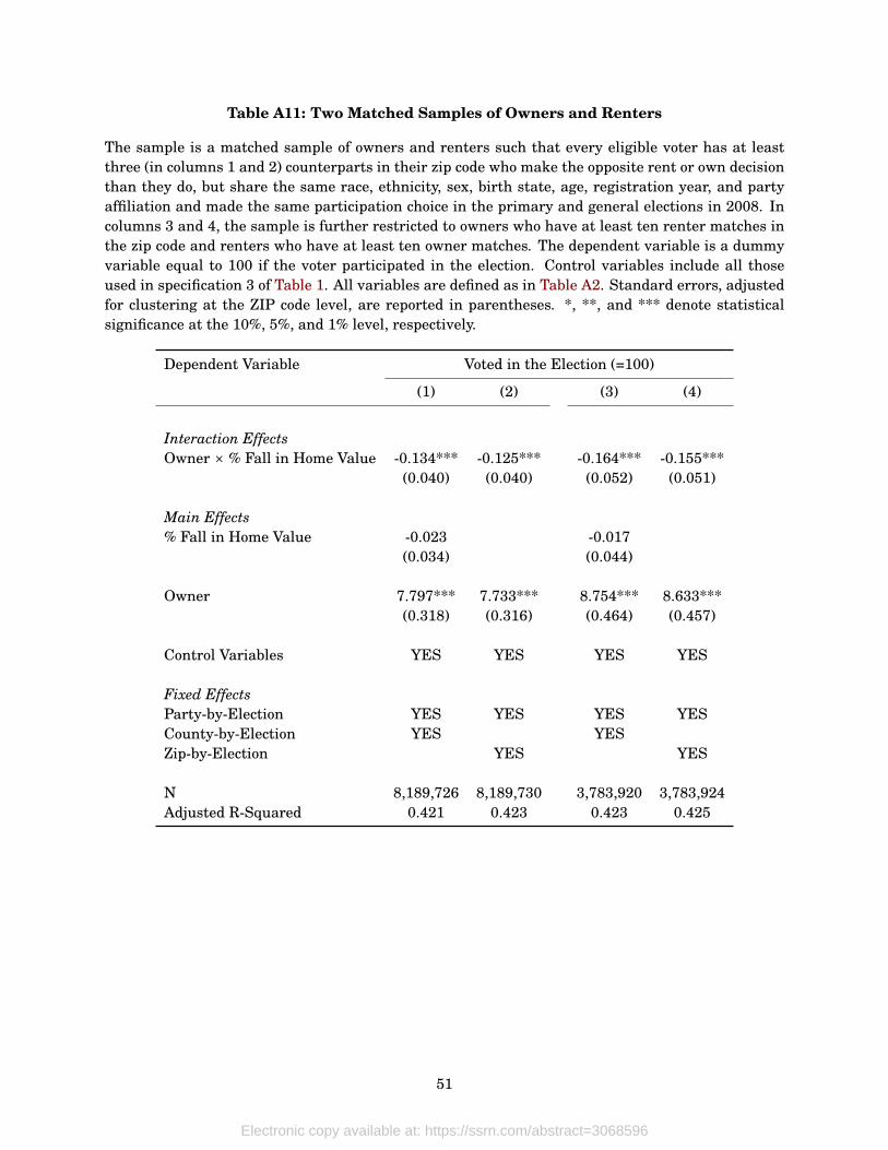
Table A11: Two Matched Samples of Owners and Renters

The sample is a matched sample of owners and renters such that every eligible voter has at leastthree (in columns 1 and 2) counterparts in their zip code who make the opposite rent or own decisionthan they do, but share the same race, ethnicity, sex, birth state, age, registration year, and partyaffiliation and made the same participation choice in the primary and general elections in 2008. Incolumns 3 and 4, the sample is further restricted to owners who have at least ten renter matches inthe zip code and renters who have at least ten owner matches. The dependent variable is a dummyvariable equal to 100 if the voter participated in the election. Control variables include all thoseused in specification 3 of Table 1. All variables are defined as in Table A2. Standard errors, adjustedfor clustering at the ZIP code level, are reported in parentheses. *, **, and *** denote statisticalsignificance at the 10%, 5%, and 1% level, respectively.


(1) (2) (3) (4)

Interaction EffectsOwner × % Fall in Home Value -0.134*** -0.125*** -0.164*** -0.155***

(0.040) (0.040) (0.052) (0.051)

Main Effects% Fall in Home Value -0.023 -0.017

(0.034) (0.044)

Owner 7.797*** 7.733*** 8.754*** 8.633***(0.318) (0.316) (0.464) (0.457)


Fixed EffectsParty-by-Election YES YES YES YESCounty-by-Election YES YESZip-by-Election YES YES


51


Table A12: Two Matched Samples of Underwater and Non-Underwater Homeowners

The sample in the first two specifications is a matched sample of underwater homeowners and home-owners with positive equity in their homes such that every eligible voter with a mortgage has atleast three (in columns 1 and 2) counterparts in their zip code who are non-underwater (underwater)if they are underwater (non-underwater), and also share the same race, ethnicity, sex, birth state,age, registration year, and party affiliation and made the same participation choice in the primaryand general elections in 2008. In columns 3 and 4, the sample is a one-to-one match of underwaterand non-underwater homeowners, matched on the same variables as above. The dependent variableis a dummy variable equal to 100 if the voter participated in the election. Control variables includeall those used in specification 3 of Table 1. All variables are defined as in Table A2. Standard er-rors, adjusted for clustering at the ZIP code level, are reported in parentheses. *, **, and *** denotestatistical significance at the 10%, 5%, and 1% level, respectively.


(1) (2) (3) (4)

Underwater (=1) -0.290** -1.592*** -0.413*** -0.739**(0.146) (0.406) (0.136) (0.315)


Fixed EffectsCounty-by-Election YES YESParty-by-Election YES YESIndividual YES YESElection YES YES

N 1,162,886 1,167,900 689,975 694,602Adjusted R-Squared 0.407 0.504 0.408 0.507

52


Table A13: Demographics of the Registered NC Voters in the Full Sample

This table presents summary statistics on the sample of all registered voters in each of the threegeneral elections in the sample. It is analogous to Table A2, but while Table A2 summarizes onlythose voters who were registered to vote and active at the same address over all elections between2008 and 2012, this table describes all voters.

Election

2008 General 2010 General 2012 General


Regsitration Year1983 or Prior 15.76% 14.79% 13.01%1984 - 1991 11.08% 10.53% 9.44%1992 - 1999 20.80% 19.16% 16.71%2000 - 2008 52.36% 47.16% 37.67%2009 or Later 0.00% 8.37% 23.18%

Birth Year1942 or Prior 16.73% 15.28% 13.15%1943 - 1958 26.71% 26.70% 25.74%1959 - 1974 30.47% 30.30% 29.33%1975 - 1990 26.09% 25.84% 25.47%1991 or Later 0.00% 1.88% 6.32%


HomeownershipRenter 39.82% 37.47% 38.08%Homeowner without Mortgage 24.27% 24.57% 23.47%Homeowner with Mortgage 35.91% 37.96% 38.44%


Among Homeowners0% ≤ Current CLTV ≤ 80% 63.45% 53.60% 51.01%80% < Current CLTV ≤ 100% 28.47% 29.35% 29.28%100% < Current CLTV 8.08% 17.05% 19.71%

N 5,847,334 5,761,055 5,980,277

53


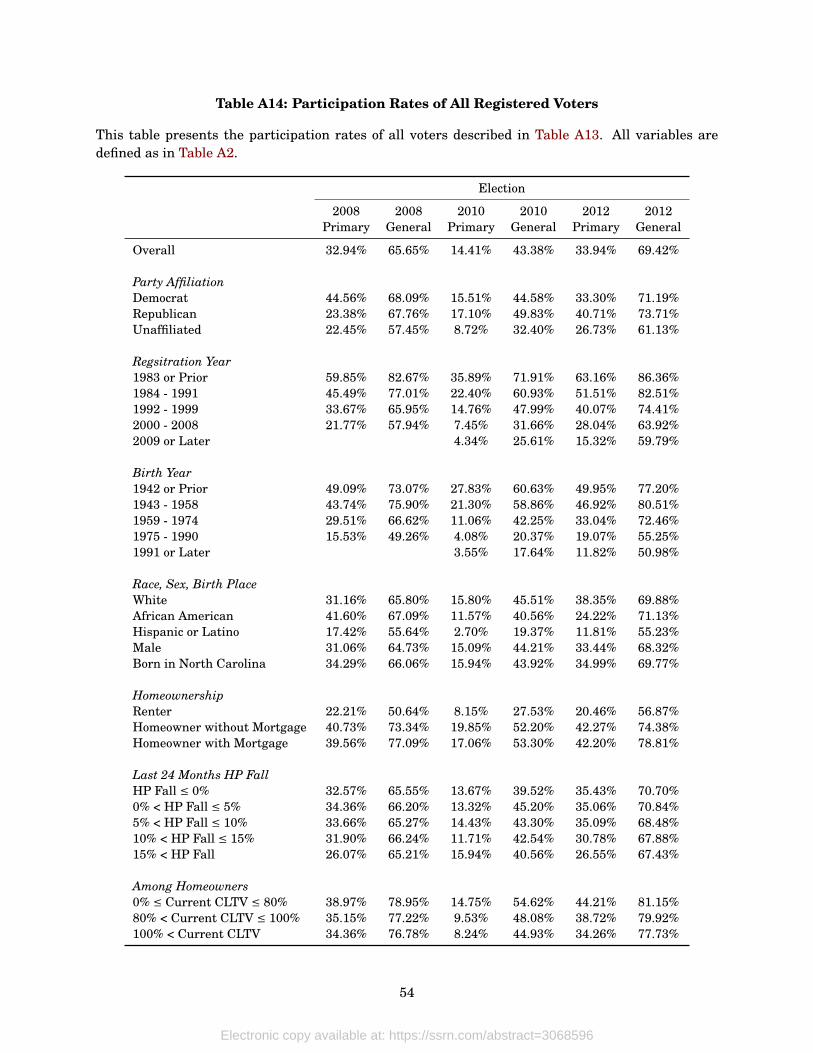
Table A14: Participation Rates of All Registered Voters

This table presents the participation rates of all voters described in Table A13. All variables aredefined as in Table A2.

Election

2008 2008 2010 2010 2012 2012Primary General Primary General Primary General

Overall 32.94% 65.65% 14.41% 43.38% 33.94% 69.42%

Party AffiliationDemocrat 44.56% 68.09% 15.51% 44.58% 33.30% 71.19%Republican 23.38% 67.76% 17.10% 49.83% 40.71% 73.71%Unaffiliated 22.45% 57.45% 8.72% 32.40% 26.73% 61.13%

Regsitration Year1983 or Prior 59.85% 82.67% 35.89% 71.91% 63.16% 86.36%1984 - 1991 45.49% 77.01% 22.40% 60.93% 51.51% 82.51%1992 - 1999 33.67% 65.95% 14.76% 47.99% 40.07% 74.41%2000 - 2008 21.77% 57.94% 7.45% 31.66% 28.04% 63.92%2009 or Later 4.34% 25.61% 15.32% 59.79%

Birth Year1942 or Prior 49.09% 73.07% 27.83% 60.63% 49.95% 77.20%1943 - 1958 43.74% 75.90% 21.30% 58.86% 46.92% 80.51%1959 - 1974 29.51% 66.62% 11.06% 42.25% 33.04% 72.46%1975 - 1990 15.53% 49.26% 4.08% 20.37% 19.07% 55.25%1991 or Later 3.55% 17.64% 11.82% 50.98%

Race, Sex, Birth PlaceWhite 31.16% 65.80% 15.80% 45.51% 38.35% 69.88%African American 41.60% 67.09% 11.57% 40.56% 24.22% 71.13%Hispanic or Latino 17.42% 55.64% 2.70% 19.37% 11.81% 55.23%Male 31.06% 64.73% 15.09% 44.21% 33.44% 68.32%Born in North Carolina 34.29% 66.06% 15.94% 43.92% 34.99% 69.77%

HomeownershipRenter 22.21% 50.64% 8.15% 27.53% 20.46% 56.87%Homeowner without Mortgage 40.73% 73.34% 19.85% 52.20% 42.27% 74.38%Homeowner with Mortgage 39.56% 77.09% 17.06% 53.30% 42.20% 78.81%

Last 24 Months HP FallHP Fall ≤ 0% 32.57% 65.55% 13.67% 39.52% 35.43% 70.70%0% < HP Fall ≤ 5% 34.36% 66.20% 13.32% 45.20% 35.06% 70.84%5% < HP Fall ≤ 10% 33.66% 65.27% 14.43% 43.30% 35.09% 68.48%10% < HP Fall ≤ 15% 31.90% 66.24% 11.71% 42.54% 30.78% 67.88%15% < HP Fall 26.07% 65.21% 15.94% 40.56% 26.55% 67.43%

Among Homeowners0% ≤ Current CLTV ≤ 80% 38.97% 78.95% 14.75% 54.62% 44.21% 81.15%80% < Current CLTV ≤ 100% 35.15% 77.22% 9.53% 48.08% 38.72% 79.92%100% < Current CLTV 34.36% 76.78% 8.24% 44.93% 34.26% 77.73%

54


Table A15: Local House Price Declines on Voter Participation, Full Sample

The dependent variable is a dummy variable equal to 100 if the voter participated in the election. All variables are defined as in Table A2.The sample includes all voters registered to vote in at least one election between 2008 and 2012. Consequently, the control variables do notinclude participation in the 2008 primary and 2008 general elections, since many of the voters were not registered to vote in those elections.Specification 1 corresponds to specification 3 from Table 1. Specification 3 corresponds to specification 3 of Table 3 and specification 5 tospecification 1 from Table 5. Standard errors, adjusted for clustering at the ZIP code level, are reported in parentheses. *, **, and ***denote statistical significance at the 10%, 5%, and 1% level, respectively.


(1) (2) (3) (4) (5) (6)

% Fall in Home Value -0.125*** -0.111*** -0.0941*** 0.027(0.027) (0.040) (0.025) (0.058)

Owner without Mortgage 8.916***0.000

Owner with Mortgage 15.23***0.000

Without Mortgage × % Fall in Home Value 0.0076 -0.0982(0.030) (0.063)

With Mortgage × % Fall in Home Value -0.0716** -0.153*(0.031) (0.078)

Underwater (=1) -0.652*** -1.378***(0.138) (0.254)

Control Variables YES YES YES YES YES YES

Fixed EffectsCounty-by-Election YES YES YESParty-by-Election YES YES YESIndividual YES YES YESElection YES YES YES

N 7,973,066 8,097,564 19,924,086 20,305,564 4,191,995 4,193,321Adjusted R-Squared 0.271 0.511 0.278 0.514 0.295 0.504

55


/abstract=3068596

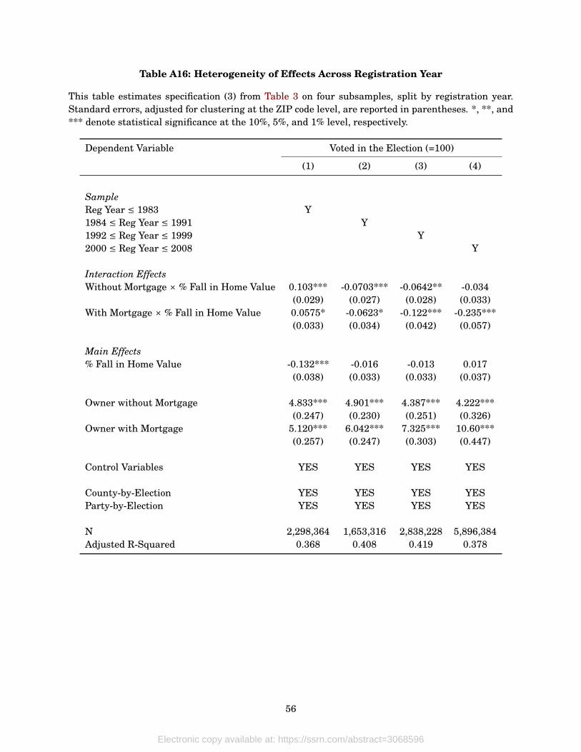
Table A16: Heterogeneity of Effects Across Registration Year

This table estimates specification (3) from Table 3 on four subsamples, split by registration year.Standard errors, adjusted for clustering at the ZIP code level, are reported in parentheses. *, **, and*** denote statistical significance at the 10%, 5%, and 1% level, respectively.


(1) (2) (3) (4)

SampleReg Year ≤ 1983 Y1984 ≤ Reg Year ≤ 1991 Y1992 ≤ Reg Year ≤ 1999 Y2000 ≤ Reg Year ≤ 2008 Y

Interaction EffectsWithout Mortgage × % Fall in Home Value 0.103*** -0.0703*** -0.0642** -0.034

(0.029) (0.027) (0.028) (0.033)With Mortgage × % Fall in Home Value 0.0575* -0.0623* -0.122*** -0.235***

(0.033) (0.034) (0.042) (0.057)

Main Effects% Fall in Home Value -0.132*** -0.016 -0.013 0.017

(0.038) (0.033) (0.033) (0.037)




County-by-Election YES YES YES YESParty-by-Election YES YES YES YES


56


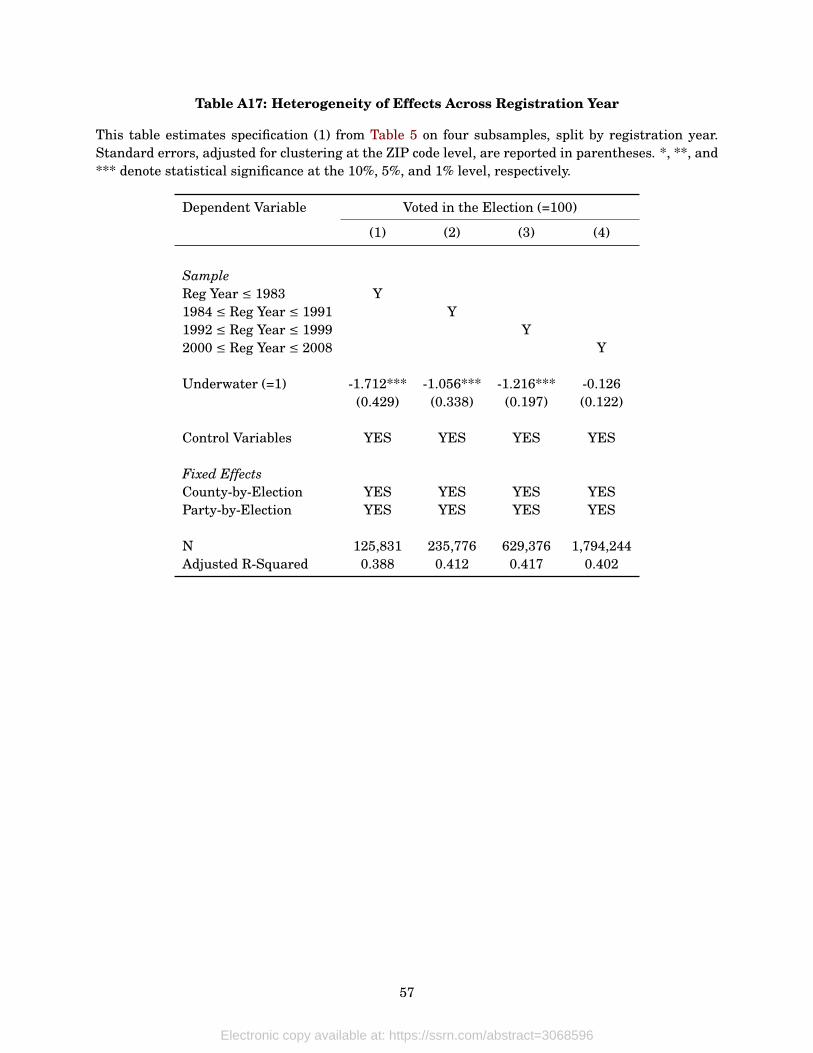
Table A17: Heterogeneity of Effects Across Registration Year

This table estimates specification (1) from Table 5 on four subsamples, split by registration year.Standard errors, adjusted for clustering at the ZIP code level, are reported in parentheses. *, **, and*** denote statistical significance at the 10%, 5%, and 1% level, respectively.


(1) (2) (3) (4)

SampleReg Year ≤ 1983 Y1984 ≤ Reg Year ≤ 1991 Y1992 ≤ Reg Year ≤ 1999 Y2000 ≤ Reg Year ≤ 2008 Y

Underwater (=1) -1.712*** -1.056*** -1.216*** -0.126(0.429) (0.338) (0.197) (0.122)


Fixed EffectsCounty-by-Election YES YES YES YESParty-by-Election YES YES YES YES

N 125,831 235,776 629,376 1,794,244Adjusted R-Squared 0.388 0.412 0.417 0.402

57


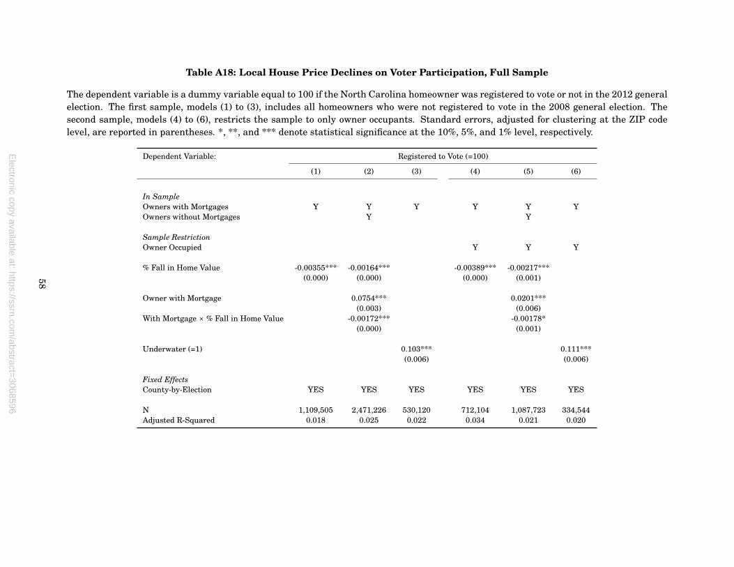
Table A18: Local House Price Declines on Voter Participation, Full Sample

The dependent variable is a dummy variable equal to 100 if the North Carolina homeowner was registered to vote or not in the 2012 generalelection. The first sample, models (1) to (3), includes all homeowners who were not registered to vote in the 2008 general election. Thesecond sample, models (4) to (6), restricts the sample to only owner occupants. Standard errors, adjusted for clustering at the ZIP codelevel, are reported in parentheses. *, **, and *** denote statistical significance at the 10%, 5%, and 1% level, respectively.

Dependent Variable: Registered to Vote (=100)

(1) (2) (3) (4) (5) (6)

In SampleOwners with Mortgages Y Y Y Y Y YOwners without Mortgages Y Y

Sample RestrictionOwner Occupied Y Y Y

% Fall in Home Value -0.00355*** -0.00164*** -0.00389*** -0.00217***(0.000) (0.000) (0.000) (0.001)

Owner with Mortgage 0.0754*** 0.0201***(0.003) (0.006)

With Mortgage × % Fall in Home Value -0.00172*** -0.00178*(0.000) (0.001)

Underwater (=1) 0.103*** 0.111***(0.006) (0.006)

Fixed EffectsCounty-by-Election YES YES YES YES YES YES

N 1,109,505 2,471,226 530,120 712,104 1,087,723 334,544Adjusted R-Squared 0.018 0.025 0.022 0.034 0.021 0.020

58


/abstract=3068596

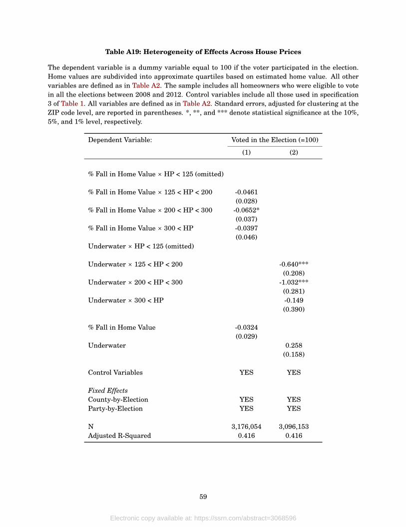
Table A19: Heterogeneity of Effects Across House Prices

The dependent variable is a dummy variable equal to 100 if the voter participated in the election.Home values are subdivided into approximate quartiles based on estimated home value. All othervariables are defined as in Table A2. The sample includes all homeowners who were eligible to votein all the elections between 2008 and 2012. Control variables include all those used in specification3 of Table 1. All variables are defined as in Table A2. Standard errors, adjusted for clustering at theZIP code level, are reported in parentheses. *, **, and *** denote statistical significance at the 10%,5%, and 1% level, respectively.


(1) (2)

% Fall in Home Value × HP < 125 (omitted)

% Fall in Home Value × 125 < HP < 200 -0.0461(0.028)

% Fall in Home Value × 200 < HP < 300 -0.0652*(0.037)

% Fall in Home Value × 300 < HP -0.0397(0.046)

Underwater × HP < 125 (omitted)

Underwater × 125 < HP < 200 -0.640***(0.208)

Underwater × 200 < HP < 300 -1.032***(0.281)

Underwater × 300 < HP -0.149(0.390)

% Fall in Home Value -0.0324(0.029)

Underwater 0.258(0.158)


Fixed EffectsCounty-by-Election YES YESParty-by-Election YES YES

N 3,176,054 3,096,153Adjusted R-Squared 0.416 0.416

59


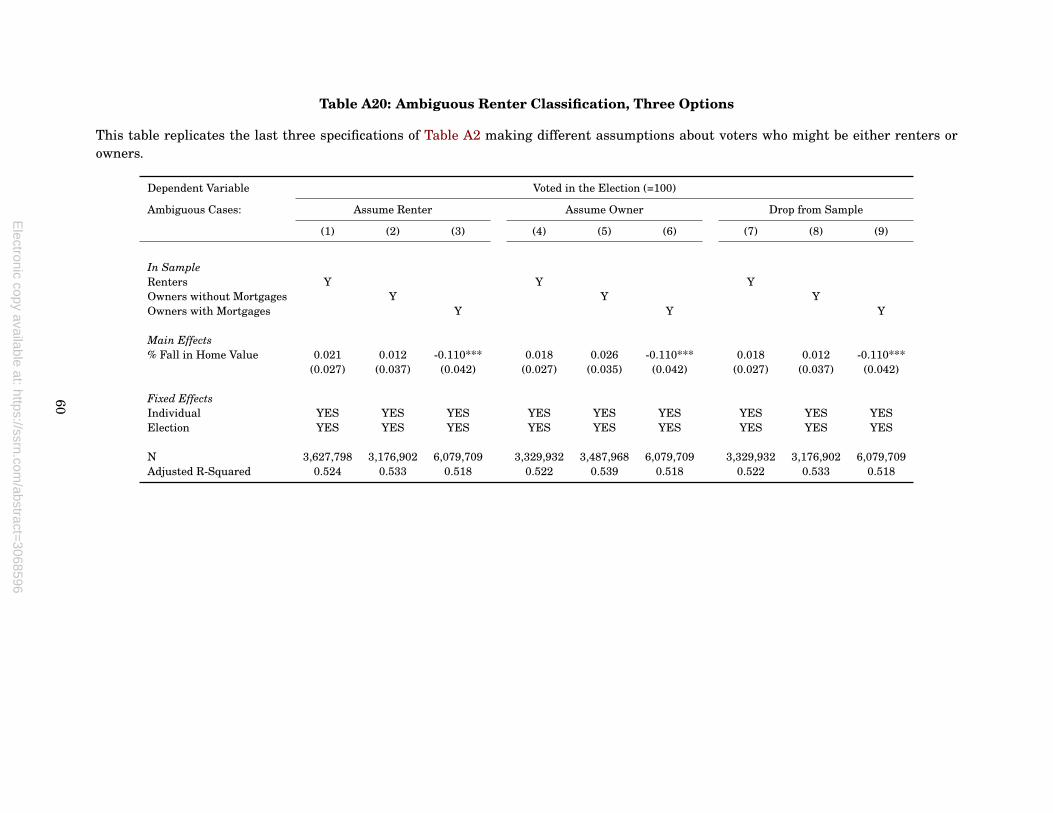
Table A20: Ambiguous Renter Classification, Three Options

This table replicates the last three specifications of Table A2 making different assumptions about voters who might be either renters orowners.


Ambiguous Cases: Assume Renter Assume Owner Drop from Sample

(1) (2) (3) (4) (5) (6) (7) (8) (9)

In SampleRenters Y Y YOwners without Mortgages Y Y YOwners with Mortgages Y Y Y

Main Effects% Fall in Home Value 0.021 0.012 -0.110*** 0.018 0.026 -0.110*** 0.018 0.012 -0.110***

(0.027) (0.037) (0.042) (0.027) (0.035) (0.042) (0.027) (0.037) (0.042)

Fixed EffectsIndividual YES YES YES YES YES YES YES YES YESElection YES YES YES YES YES YES YES YES YES

N 3,627,798 3,176,902 6,079,709 3,329,932 3,487,968 6,079,709 3,329,932 3,176,902 6,079,709Adjusted R-Squared 0.524 0.533 0.518 0.522 0.539 0.518 0.522 0.533 0.518

60


/abstract=3068596

B Dataset Construction and Description

To calculate current CLTV, I first calculate the outstanding loan balance by assuming that the house-

hold repays following a standard 30 year fixed-rate mortgage amortization schedule and is being

charged the interest rate that was prevailing in North Carolina the month the loan was originated.24

I further assume that refinance loans replace the outstanding loan and that home equity loans and

home equity lines of credit are immediately drawn down, added to the outstanding balance, and paid

back over ten years. To calculate the home’s value I take the most recent purchase price and appre-

ciate it by the same amount as the median house price in its zip code. I then divide the outstanding

mortgage balance by the current value of the home to calculate the current CLTV. Table A2 shows

that the share of households underwater, with CLTVs above 100%, increased from 7% in 2008 to 14%

in 2010 and then again to 16% in 2012.

To merge the voter rolls data with the deeds data, I begin by requiring first name, middle initial,

last name, house number, street name, and zip code to be identical. I then take the unmatched

voters and look for a match by slightly relaxing the matching criteria. For example, I allow matches

between observations where the voter has a middle initial and the property owner does not (this

captures slight discrepancies in what each data source is recording), observations where the last

name or street name are very close (this solves for both typos and ambiguous street names, e.g.

Highway 131 vs HWY 131), and matching first name and exact address (which captures spouses). I

call the unmatched voters renters unless they are at some other point identified as owners at that

same address in the deeds data. I do this to capture spouses that are sometimes included on the deed

and other times not.

The primary limitation of my algorithm is that owner-occupants who are never on the deed are

incorrectly classified as renters when, in reality, they are homeowners. I do observe them, but I

cannot be sure if they are significant others who informally share ownership with the deedholder

(informal since they are not on the deed), or if they are roommates or children who have no ownership

stake in the property. A related limitation is that if legal ownership of the same voter living at the

same address really does change I will incorrectly call them owners the whole time. This might

happen if the voter stays at the same address but ownership is transferred to a family member, if

24See https://www.fhfa.gov/DataTools/Downloads/Pages/Monthly-Interest-Rate-Data.aspx for this data.

61


https://www.fhfa.gov/DataTools/Downloads/Pages/Monthly-Interest-Rate-Data.aspx for this data

the voter sells the property to a landlord but continues to live there, or if the voter purchases the

property from their landlord. This ambiguity arises in approximately 2.5% of observations. Table

A20 replicates the main results assuming these ambiguous voters are renters, are owners, or are

dropped from the sample. The main result that households with mortgages are especially affected is

unchanged. Specification (3), (6), and (9) are identical by construction since this ambiguity does not

affect voters with mortgages.

A second limitation is that individuals living in North Carolina who are not registered to vote do

not appear in the sample, even if they own property in North Carolina. It is tempting to include all

CoreLogic homeowners in the final sample, but I cannot be sure that they are allowed to register to

vote in North Carolina. There are two reasons this might be the case. First, homeowners who are not

owner-occupants are not eligible to vote at that address. These could be investors / vacation home

owners who live in another state and are registered there or live somewhere else in North Carolina

and are registered at that address. Second, even if I could be sure about occupancy, homeowners who

are not US citizens are also not eligible to vote. I omit these homeowners from the sample which

means I cannot answer questions about the choice to register, since I cannot observe the set of people

eligible to register. In Section 5.5, I explore this sample of North Carolina homeowners not registered

to vote and the effects house price drops have on registration.

C Other Implied Aggregate Effects

A first, naive back-of-the-envelope calculation uses the estimated effect of house price falls on par-

ticipation from Table 1 and multiplies that estimate by the average fall in house prices in North

Carolina. Using this strategy, I estimate that house price declines caused approximately 35,000

abstentions in each of the 2010 elections, 37,000 abstentions in the 2012 primary, and 25,000 ab-

stentions in the 2012 general for a total of 132,000 abstentions.25 This translates to turnout being

between 4 percent lower (in the 2010 primary) and 0.6 percent lower (in the 2012 general) than it

would have been in the counter-factual world where house prices did not go down. Overall, house

price declines decreased participation by 1.5 percent.26 This naive strategy assumes both a linear

25For example, in 2010 there were 6,000,000 registered voters and the average average fall in house prices was 7%leading to 6m × 7 × .000835 abstentions.

26860,000 voters participated in the 2010 primary, 4,165,000 in the 2012 general, and 9,669,000 over all four elections.

62


relationship between house price falls and abstention and that effect sizes are the same for home-

owners and renters.

My results from Table 2 allow me to be more precise. Households experiencing drops in local

house prices of more than 15% were 1.9 percentage points less likely to vote, those experiencing drops

of between 10 and 15 percent were 1.1 percentage points less likely to vote, and those experiencing

falls of less than 10% were not significantly affected. Using these estimates I calculate that, in North

Carolina, house price falls during the recession caused 17,650 abstentions in the 2010 elections

and 9,200 abstentions in the 2012 elections for a total of 53,700 abstentions over the four recession

elections.27 This strategy, though more refined than the previous one, still assumes that effect sizes

were common to all registered voters, something Table 3 clearly refutes.

Households with mortgages, households without mortgages, and renters are differentially af-

fected by a common fall in house prices, and the back-of-the-envelope strategy should reflect this.

Specifically, it is only homeowners with mortgages whose participation is affected when house prices

decline. This group experienced house price falls of 7.1, 6.7, 6.9, and 4.6 percent leading into the

four national elections in the sample. Using these observed falls along with the effects estimated

in Table 3, I conclude that house price falls explain 25,000 abstentions in the 2010 primary, and

24,000, 25,500, and 17,000 abstentions in the next three elections, for a total of 91,500 abstentions.28

In short, voter turnout was no lower among renters and equity rich homeowners than it would have

been in the absence of collapsing house prices, but 2.1 percent lower among leveraged homeowners.29

This matters because officials are elected by those who vote and elected officials are inclined to push

policies their voters prefer (Cascio and Washington, 2013; Fujiwara, 2015). The implication, then, is

that the policy landscape changed in favor of renters and equity-rich homeowners – as compared to

leveraged homeowners – more than it might have had house prices not collapsed.

271,107,000 voters experiencing falls between 10% and 15% × .011 + 288,000 over 15% × .019 in 2010 and, in 2012,471,000 × .011 + 210,500 × .019.

28For example, in the 2010 primary there were 2,200,000 homeowners with mortgages registered to vote and the averagefall in house prices for them was 7.1% leading to 2.2m × 7.1 × (.00143+.00018) abstentions.

2991,500 abstentions among homeowners with mortgages compared to the 4,313,000 eligible voters with mortgages whoparticipated in the 2010 and 2012 midterm and general elections and the 8,948,320 mortgaged homeowners who couldhave.

63


Documents

Does Household Finance Affect the Political Process