Does Inequality Benefit Growth? New EvidenceUsing A Panel VAR Approach

Marcelo Eduardo Alves da Silva∗,a

aDepartment of Economics and PIMES, Universidade Federal de Pernambuco, Brazil

July, 2017

AbstractIn this paper, we investigate the dynamic relationship between economic growth and in-come inequality, an issue that has not found yet a clear consensus in the literature. Inparticular, we implement a panel VAR approach, using state-level data for Brazil, to as-sess the dynamic effects of inequality on growth and vice versa. We show that inequalityshocks lead to higher economic growth, therefore supporting the view that, in poor coun-tries, higher inequality does benefit economic growth. We also present evidence that highergrowth leads to lower income inequality, consequently pursuing growth enhancing policiesshould be translated not only in higher growth, but also in better income distribution. Ourresults are robust to different inequality measures and also when we include a measure ofhuman capital accumulation.

Keywords: Income inequality; economic growth; panel var.JEL Classification: O43, C33.

ResumoNeste trabalho, investigamos a relação dinâmica entre crescimento econômico e desigual-dade de renda, uma questão que ainda não encontrou um consenso claro na literatura.Em particular, implementamos uma abordagem VAR Painel, usando dados estaduais parao Brasil, para avaliar os efeitos dinâmicos da desigualdade no crescimento e vice-versa.Mostramos que os choques de desigualdade levam ao crescimento econômico mais ele-vado, sustentando, portanto, a opinião de que, nos países pobres, uma maior desigualdadebeneficia o crescimento econômico. Também apresentamos evidências de que um maiorcrescimento leva a uma menor desigualdade de renda, consequentemente, ao se buscarpolíticas que beneficiem o crescimento, os resultados devem ser traduzidos não apenas emmaior crescimento, mas também em uma melhor distribuição de renda. Nossos resultadossão robustos para diferentes medidas de desigualdade e também quando incluímos umamedida de acumulação de capital humano.

Palavras-chave: Desigualdade de Renda; crescimento econômico; VAR em painel.Classificação JEL: O43, C33.

Área ANPEC: 6 - Crescimento, Desenvolvimento Econômico e Instituições

∗Corresponding author: Departamento de Economia, CCSA, Universidade Federal de Pernambuco, Avenidados Economistas, S/N, 50740-580, Recife, Brazil. � marcelo.easilva@ufpe.br. We thank..... The usualdisclaimer applies.

1 Introduction

The relationship between income inequality and economic growth is a long standing issue inMacroeconomics. On the one hand, some authors have found that higher income inequality isbeneficial to growth (Partridge, 1997; Galor & Tsiddon, 1997; Li & Zou, 1998; Forbes, 2000) andmore recently Brueckner & Lederman (2015) and Cavalcanti & Giannitsarou (2016). On theother hand, there is evidence of a negative relationship with higher inequality being associatedwith lower growth (Alesina & Perotti, 1996; Persson & Tabellini, 1994; Atems & Jones, 2015).In this paper, we explore the dynamic relationship between income inequality and economicgrowth, using state-level data for Brazil, a country known by its high level of income disparities.In particular, we investigate what are the effects of shocks to income inequality on growth andvice versa.

In order to investigate this issue, we employ a Panel Vector Autoregression (PVAR) approachand estimate a bivariate PVAR using a measure of income inequality (Gini coefficient) andincome data (real GDP per capita). As in traditional Vector Auto-Regressive (VAR) models,the PVAR model is quite flexible and allow us to treat both variables as endogenous. However,PVAR models have an additional advantage over traditional VARs, the possibility to accountfor time invariant characteristics intrinsic to each unit in our sample. Moreover, given the shorttime length of our data set, this methodology exploits the panel structure of the data (short Tand large N) that is not reliable in a traditional VAR estimation. Orthogonal impulse-responsefunctions (IRFs) are obtained by means of a triangular identification scheme by assuming thatreal output per capita does not respond contemporaneously to inequality shocks.1

Our results show that after an inequality shock the growth rate of real GDP per capitaimproves and hence higher inequality is beneficial to growth.The effects on the growth rate lastfor at least 3 years after the initial shock, changing real GDP per capita permanently (leveleffect).2 On the other hand, an income shock (i.e. higher GDP growth) is followed by betterincome distribution (i.e. after a GDP shock income inequality declines). These results arerobust when we use a different inequality measure (e.g. Theil Index).

We extend our analysis by estimating a three-variable PVAR to include a measure of humancapital. We do this for two purposes. First, to capture the idea that higher economic growthmay lower income inequality through higher human capital accumulation (Brueckner et al.,2015).3 Second, adding a measure of human capital allows us to investigate whether the effectsof inequality shocks are indeed a result of a third factor, in our case, shocks to human capital.Our results are robust to introducing human capital.

This paper is related, more directly, to the branch of the literature that investigates theempirical relationship between income inequality and economic growth (Atems & Jones, 2015;Brueckner et al., 2015; Brueckner & Lederman, 2015). Atems & Jones (2015) also employ aPVAR model and show that higher inequality reduces income level and growth in US states.Brueckner et al. (2015), using a panel of 154 countries spanning 1960-2007, show that highereconomic growth is associated with lower inequality. Brueckner & Lederman (2015) estimatesthe effect of income inequality on real gross domestic product per capita using a panel of 104countries during the period 1970–2010. They find that, on average, income inequality has a1 We will discuss the validity of this restriction in section 3.2 Galor & Zeira (1993) propose a model where under credit market imperfections and indivisibilities in invest-ment in human capital, higher inequality affects real GDP per capita positively in the short run as well as inthe long run.

3For instance, Galor & Zeira (1993) argues that, when credit markets are imperfect, higher aggregate incomeare associated with lower inequality. However, the channel through which the effects of higher income aretransmitted to inequality is through higher physical capital accumulation.

2

significant negative effect on gross domestic product per capita growth and the long-run levelof gross domestic product per capita. However, they show that the impact differ by the levelof economic development. In particular, in poor countries, income inequality has a significantpositive effect on gross domestic product per capita.

The results that higher income inequality can be beneficial to economic growth are inline with the theoretical work by Galor & Zeira (1993). They show that the relationshipbetween inequality and aggregate output in the presence of credit market imperfections andindivisibilities in human capital investment varies across countries initial income levels. While,in rich economies, we should expect a negative relationship between inequality and growth, inpoor countries, higher income inequality may be associated with higher economic growth andhigher real GDP per capita.4 This is the result presented in Brueckner & Lederman (2015)and also showed in this paper. Cavalcanti & Giannitsarou (2016), using a concept of network,show that the relationship between growth and inequality is also positive for a given networkstructure. They show that when the network cohesion is low, the more likely it is to have highgrowth and inequality in the long run.5

The remainder of the paper is organized as follows. In section 2 we give the details onthe dataset used. In section 3 we present our empirical methodology. Section 4 discusses theresults. Finally, conclusions are presented in section 5.

2 Data

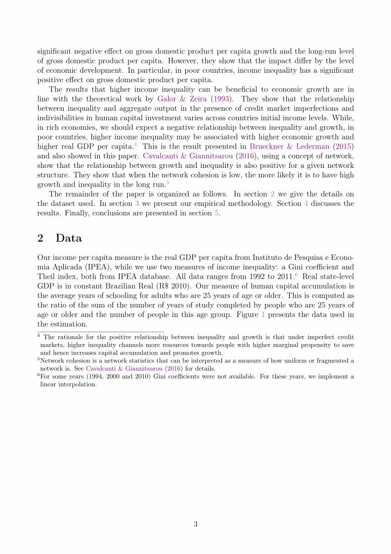
Our income per capita measure is the real GDP per capita from Instituto de Pesquisa e Econo-mia Aplicada (IPEA), while we use two measures of income inequality: a Gini coefficient andTheil index, both from IPEA database. All data ranges from 1992 to 2011.6 Real state-levelGDP is in constant Brazilian Real (R$ 2010). Our measure of human capital accumulation isthe average years of schooling for adults who are 25 years of age or older. This is computed asthe ratio of the sum of the number of years of study completed by people who are 25 years ofage or older and the number of people in this age group. Figure 1 presents the data used inthe estimation.4 The rationale for the positive relationship between inequality and growth is that under imperfect creditmarkets, higher inequality channels more resources towards people with higher marginal propensity to saveand hence increases capital accumulation and promotes growth.

5Network cohesion is a network statistics that can be interpreted as a measure of how uniform or fragmented anetwork is. See Cavalcanti & Giannitsarou (2016) for details.

6For some years (1994, 2000 and 2010) Gini coefficients were not available. For these years, we implement alinear interpolation.

3

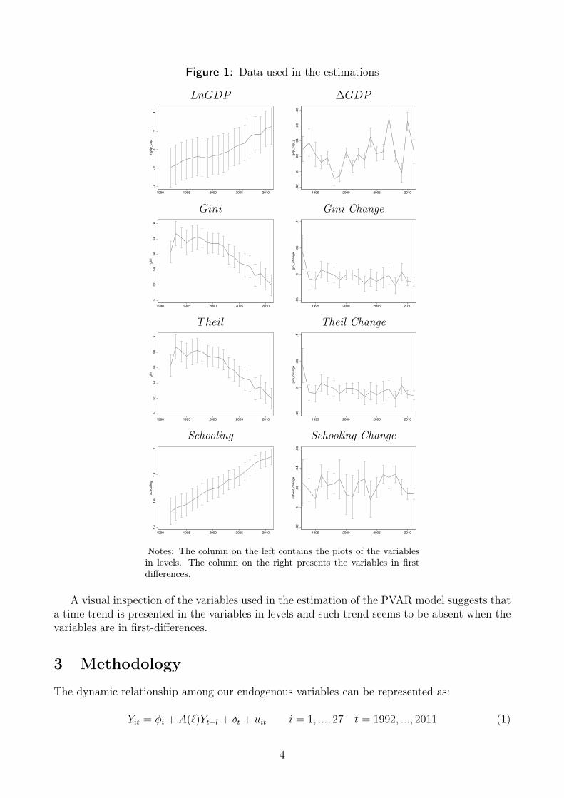
Figure 1: Data used in the estimations

LnGDP ∆GDP

-.4-.2

0.2

.4lngdp_cap

1990 1995 2000 2005 2010

-.02

0.02

.04

.06

.08

gdp_cap_g

1995 2000 2005 2010

Gini Gini Change

.5.52

.54

.56

.58

.6gini

1990 1995 2000 2005 2010

-.05

0.05

.1gini_change

1995 2000 2005 2010

Theil Theil Change

.5.52

.54

.56

.58

.6gini

1990 1995 2000 2005 2010

-.05

0.05

.1gini_change

1995 2000 2005 2010

Schooling Schooling Change

1.4

1.6

1.8

2schooling

1990 1995 2000 2005 2010

-.02

0.02

.04

.06

school_change

1995 2000 2005 2010

Notes: The column on the left contains the plots of the variablesin levels. The column on the right presents the variables in firstdifferences.

A visual inspection of the variables used in the estimation of the PVAR model suggests thata time trend is presented in the variables in levels and such trend seems to be absent when thevariables are in first-differences.

3 Methodology

The dynamic relationship among our endogenous variables can be represented as:

Yit = φi + A(`)Yt−l + δt + uit i = 1, ..., 27 t = 1992, ..., 2011 (1)

4

where Yit = [∆GDPit, Giniit]′ is a κ×1 vector of endogenous variables for unit (state) i at time

t, φi is a κ×1 vector of time-invariant state fixed effects, δt represents unobservable time effects,A(`) are κ × κ matrices of lagged coefficients. The fixed effects capture any differences acrossstates that are time invariant (e.g. cost of living, climate, etc.). Finally, uit ∼ iid(0,Σu) is aκ× 1 vector of reduced form idiosyncratic disturbances with a nonsingular variance-covariancematrix, Σu.

Pooled fixed effects estimation is one possible way to estimate the parameters of the model(1). However, even when N is large, but T is fixed, the pooled estimator is biased. Weimplement a "Helmet procedure" and employ a GMM approach of Arellano & Bover (1995),which is consistent even when T is small.7. The procedure implements a transformation toeliminate the individual fixed-effects. Therefore, before estimation, we rewrite equation (1) interms of forward orthogonal deviations denoted by:

¯̄yit = (yit − yit)

√Tit

Tit + 1(2)

where Tit is the number of available future observations for state i at time t and yit is its average.Applying this transformation to our endogenous variables, allow us to rewrite the system (1)as:

¯̄Yit = A(`) ¯̄Yt−1 + δt + uit i = 1, ..., 27 t = 1992, ..., 2011 (3)

The transformed variables in Equation (3) are orthogonal to the original variables and hencethe latter can be used as instruments.

To achieve identification, we assume real GDP per capita (or its growth rate) does notrespond contemporaneously to an inequality shock within the year. Therefore the variance-covariance matrix of the residuals, Σu, takes the form of a lower-triangular matrix with ∆GDPentering first in the Yi,t vector. This identifying restriction is justified based on the fact thatreal income is used in the computation of the Gini coefficients, so we would expect that anychange in real income will be translated to the Gini coefficient contemporaneously, but not thereverse. That is, changes in Gini coefficient will take at least one year to affect real income(Atems & Jones, 2015).

For the purpose of recovering impulse response functions, equation (3) can be rewritten asB(`) ¯̄Yit = uit, where B(`) = (Ik − A(`)). As long as all eingenvalues of A(`) have modulus lessthan 1, B(`) satisfies the stability condition and hence is invertible. Therefore, we can obtaina MA representation of the PVAR model

¯̄Yi,t = Θ(`)uit, (4)

where Θ(`) =∑∞

j=0 Θjlj ≡ B(`)−1. The disturbances uit are correlated contemporaneously and

hence we implement a Cholesky decomposition on Σu = P ′P , where P is a lower-triangularmatrix, such that it is possible to orthogonalize disturbances as P−1uit ≡ eit. The vector eit willbe the orthogonalized disturbances, which it will give us the orthogonalized impulse-responsefunctions.7The bias is due to the fact that unit specific intercepts, φi, are correlated with the error term.

5

4 Results

First, we present the results for a variety of panel unit tests.8 Second, we present the ImpulseResponse Functions (IRFs) from our baseline bivariate PVAR specification. Finally, we extendour analysis by introducing a measure of human capital. We do this for two purposes. First,to capture the idea that higher economic growth may lower income inequality through higherhuman capital accumulation (Brueckner et al., 2015). Second, to investigate whether the effectsof inequality shocks are indeed a result of a third factor, in our case, shocks to human capital.

4.1 Panel Unit Root Tests

Table 1 presents the results of different panel unit root tests. Testing unit roots in context ofpanel data is not as straightforward as in usual time series analysis, but the idea is similar.9Consider a variable that can be represented by a single panel-data model with a first-orderautoregressive representation such as:

xit = ρixi,t−1 +W ′itγi + εit (5)

where xit is the variable being tested, the term Wit can represent panel-specific means and/ora time trend. Typically, most tests evaluates the null H0 : ρi = 1. However, a more commonapproach is to rewrite the test equation 5 as:

∆xit = ρixi,t−1 +W ′itγi + εit (6)

and to test, alternatively, H0 : ρi = 0, where ∆xit is the variable being tested in first differences.The specific form of the null hypothesis varies across test, while in Levin-Lin-Chu (LLC) test,Harris-Tzavalis (HT) test, Im-Pesaran-Shin (IPS) test and Fisher (ADF type) test the null isof nonstationarity, in Hadri’s test, the null is that all panels are stationary.

We perform each test on the level and on the first difference of each variable in our sample.Therefore, in deciding whether the variable will enter the PVAR model in level or in firstdifferences we take into account the panel unit root test results. Additionally, we also computethe eigenvalues of the A(`) matrix to check whether the PVAR model has a stable movingaverage representation.

A visual inspection of Figure 1 suggests a time trend is present in all variables in levels, soin performing unit root tests we allow for a time trend, while the lag length choices are basedon the Akaike Information Criterion when possible. Table 1 presents the results of the panelunit root tests.8 We also check the stability condition, i.e., whether the eingenvalues of the matrix of estimated coefficients arestrictly less than one. Figure 9 in appendix presents a graphical representation of this condition.

9 For a recent survey about panel unit root tests and how to interpret these tests in context of panel data seePesaran (2012).

6

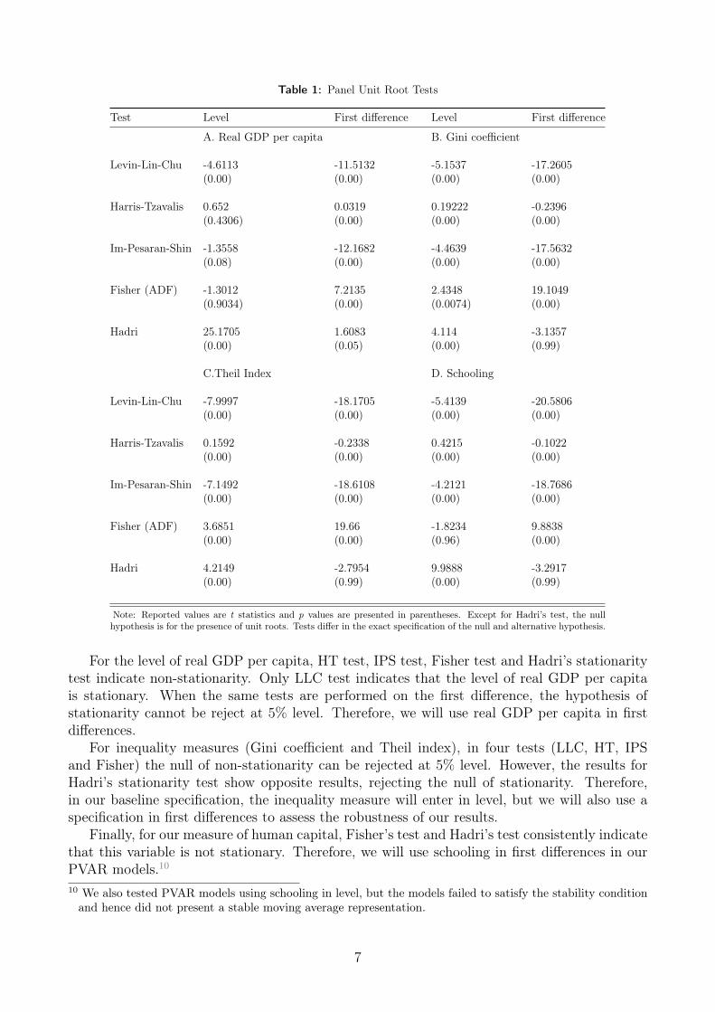
Table 1: Panel Unit Root Tests

Test Level First difference Level First difference

A. Real GDP per capita B. Gini coefficient

Levin-Lin-Chu -4.6113 -11.5132 -5.1537 -17.2605(0.00) (0.00) (0.00) (0.00)

Harris-Tzavalis 0.652 0.0319 0.19222 -0.2396(0.4306) (0.00) (0.00) (0.00)

Im-Pesaran-Shin -1.3558 -12.1682 -4.4639 -17.5632(0.08) (0.00) (0.00) (0.00)

Fisher (ADF) -1.3012 7.2135 2.4348 19.1049(0.9034) (0.00) (0.0074) (0.00)

Hadri 25.1705 1.6083 4.114 -3.1357(0.00) (0.05) (0.00) (0.99)

C.Theil Index D. Schooling

Levin-Lin-Chu -7.9997 -18.1705 -5.4139 -20.5806(0.00) (0.00) (0.00) (0.00)

Harris-Tzavalis 0.1592 -0.2338 0.4215 -0.1022(0.00) (0.00) (0.00) (0.00)

Im-Pesaran-Shin -7.1492 -18.6108 -4.2121 -18.7686(0.00) (0.00) (0.00) (0.00)

Fisher (ADF) 3.6851 19.66 -1.8234 9.8838(0.00) (0.00) (0.96) (0.00)

Hadri 4.2149 -2.7954 9.9888 -3.2917(0.00) (0.99) (0.00) (0.99)

Note: Reported values are t statistics and p values are presented in parentheses. Except for Hadri’s test, the nullhypothesis is for the presence of unit roots. Tests differ in the exact specification of the null and alternative hypothesis.

For the level of real GDP per capita, HT test, IPS test, Fisher test and Hadri’s stationaritytest indicate non-stationarity. Only LLC test indicates that the level of real GDP per capitais stationary. When the same tests are performed on the first difference, the hypothesis ofstationarity cannot be reject at 5% level. Therefore, we will use real GDP per capita in firstdifferences.

For inequality measures (Gini coefficient and Theil index), in four tests (LLC, HT, IPSand Fisher) the null of non-stationarity can be rejected at 5% level. However, the results forHadri’s stationarity test show opposite results, rejecting the null of stationarity. Therefore,in our baseline specification, the inequality measure will enter in level, but we will also use aspecification in first differences to assess the robustness of our results.

Finally, for our measure of human capital, Fisher’s test and Hadri’s test consistently indicatethat this variable is not stationary. Therefore, we will use schooling in first differences in ourPVAR models.10

10 We also tested PVAR models using schooling in level, but the models failed to satisfy the stability conditionand hence did not present a stable moving average representation.

7

4.2 Impulse Responses

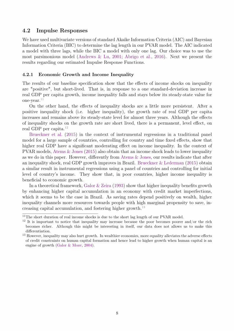
We have used multivariate versions of standard Akaike Information Criteria (AIC) and BayesianInformation Criteria (BIC) to determine the lag length in our PVAR model. The AIC indicateda model with three lags, while the BIC a model with only one lag. Our choice was to use themost parsimonious model (Andrews & Lu, 2001; Abrigo et al., 2016). Next we present theresults regarding our estimated Impulse Response Functions.

4.2.1 Economic Growth and Income Inequality

The results of our baseline specification show that the effects of income shocks on inequalityare "positive", but short-lived. That is, in response to a one standard-deviation increase inreal GDP per capita growth, income inequality falls and stays below its steady-state value forone-year.11

On the other hand, the effects of inequality shocks are a little more persistent. After apositive inequality shock (i.e. higher inequality), the growth rate of real GDP per capitaincreases and remains above its steady-state level for almost three years. Although the effectsof inequality shocks on the growth rate are short lived, there is a permanent, level effect, onreal GDP per capita.12

Brueckner et al. (2015) in the context of instrumental regressions in a traditional panelmodel for a large sample of countries, controlling for country and time fixed effects, show thathigher real GDP have a significant moderating effect on income inequality. In the context ofPVAR models, Atems & Jones (2015) also obtain that an income shock leads to lower inequalityas we do in this paper. However, differently from Atems & Jones, our results indicate that afteran inequality shock, real GDP growth improves in Brazil. Brueckner & Lederman (2015) obtaina similar result in instrumental regressions using a panel of countries and controlling for initiallevel of country’s income. They show that, in poor countries, higher income inequality isbeneficial to economic growth.

In a theoretical framework, Galor & Zeira (1993) show that higher inequality benefits growthby enhancing higher capital accumulation in an economy with credit market imperfections,which it seems to be the case in Brazil. As saving rates depend positively on wealth, higherinequality channels more resources towards people with high marginal propensity to save, in-creasing capital accumulation, and fostering higher growth.13

11The short duration of real income shocks is due to the short lag length of our PVAR model.12 It is important to notice that inequality may increase because the poor becomes poorer and/or the richbecomes richer. Although this might be interesting in itself, our data does not allows us to make thisdifferentiation.

13 However, inequality may also hurt growth. In wealthier economies, more equality alleviates the adverse effectsof credit constraints on human capital formation and hence lead to higher growth when human capital is anengine of growth (Galor & Moav, 2004).

8

Figure 2: Growth and Inequality: Impulse-Responses

Response of Response of∆GDP Gini

Impu

lseon

∆GDP

0

.01

.02

.03

0 5-.003

-.002

-.001

0

.001

0 5

Impu

lseon

Gini

0

.005

.01

0 50

.005

.01

.015

.02

0 5

Notes: The column on the left contains the plots of the responses from∆GDP to a one standard deviation shock in each indicated variable. Thecolumn on the right are the responses from Gini to a shock of one standarddeviation in each indicated variable. The shadowed area represent the 68%confidence interval using a Monte Carlo procedure with 500 replications.

Using our inequality measure in first differences does not alter the results. In response toan inequality shock (a shock to its growth rate), the growth rate of real GDP per capita stillincreases. Similarly, in response to an income shock, the growth rate of the Gini coefficientfalls. Figure 3 presents these results.

9

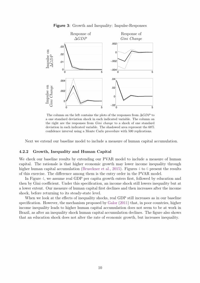
Figure 3: Growth and Inequality: Impulse-Responses

Response of Response of∆GDP Gini Change

Impu

lseon

∆GDP

0

.01

.02

.03

0 5-.004

-.002

0

.002

0 5

Impu

lseon

Gin

iC

hang

e

0

.002

.004

0 5-.02

0

.02

.04

0 5

The column on the left contains the plots of the responses from ∆GDP toa one standard deviation shock in each indicated variable. The column onthe right are the responses from Gini change to a shock of one standarddeviation in each indicated variable. The shadowed area represent the 68%confidence interval using a Monte Carlo procedure with 500 replications.

Next we extend our baseline model to include a measure of human capital accumulation.

4.2.2 Growth, Inequality and Human Capital

We check our baseline results by extending our PVAR model to include a measure of humancapital. The rationale is that higher economic growth may lower income inequality throughhigher human capital accumulation (Brueckner et al., 2015). Figures 4 to 6 present the resultsof this exercise. The difference among them is the entry order in the PVAR model.

In Figure 4, we assume real GDP per capita growth enters first, followed by education andthen by Gini coefficient. Under this specification, an income shock still lowers inequality but ata lower extent. Our measure of human capital first declines and then increases after the incomeshock, before returning to its steady-state level.

When we look at the effects of inequality shocks, real GDP still increases as in our baselinespecification. However, the mechanism proposed by Galor (2011) that, in poor countries, higherincome inequality leads to higher human capital accumulation does not seem to be at work inBrazil, as after an inequality shock human capital accumulation declines. The figure also showsthat an education shock does not alter the rate of economic growth, but increases inequality.

10

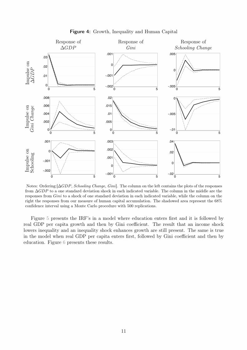
Figure 4: Growth, Inequality and Human Capital

Response of Response of Response of∆GDP Gini Schooling Change

Impu

lseon

∆GDP

0

.01

.02

.03

0 5-.002

-.001

0

.001

0 5-.005

0

.005

0 5

Impu

lseon

Gin

iC

hang

e

0

.002

.004

.006

.008

0 50

.005

.01

.015

.02

0 5-.01

-.005

0

0 5

Impu

lseon

Scho

oling

-.002

-.001

0

.001

0 5-.001

0

.001

.002

.003

0 5-.02

0

.02

.04

0 5

Notes: Ordering:[∆GDP , Schooling Change, Gini ]. The column on the left contains the plots of the responsesfrom ∆GDP to a one standard deviation shock in each indicated variable. The column in the middle are theresponses from Gini to a shock of one standard deviation in each indicated variable, while the column on theright the responses from our measure of human capital accumulation. The shadowed area represent the 68%confidence interval using a Monte Carlo procedure with 500 replications.

Figure 5 presents the IRF’s in a model where education enters first and it is followed byreal GDP per capita growth and then by Gini coefficient. The result that an income shocklowers inequality and an inequality shock enhances growth are still present. The same is truein the model when real GDP per capita enters first, followed by Gini coefficient and then byeducation. Figure 6 presents these results.

11

Figure 5: Growth, Inequality and Human Capital

Response of Response of Response of∆GDP Gini Schooling Change

Impu

lseon

∆GDP

0

.01

.02

.03

0 5-.002

-.001

0

.001

0 5

0

.002

.004

0 5

Impu

lseon

Gin

iC

hang

e

0

.002

.004

.006

.008

0 50

.005

.01

.015

.02

0 5-.01

-.005

0

0 5

Impu

lseon

Scho

oling

-.004

-.002

0

.002

0 5-.001

0

.001

.002

.003

0 5-.02

0

.02

.04

0 5

Notes: Ordering:[Schooling Change, ∆GDP , Gini ]. The column on the left contains the plots of the responsesfrom ∆GDP to a shock of one standard deviation in each indicated variable. The column on the right arethe responses from Theil to a shock of one standard deviation in each indicated variable. The solid linescorrespond to the median responses to the shocks in a ten period horizon and the dashed lines are 68%confidence interval.

12

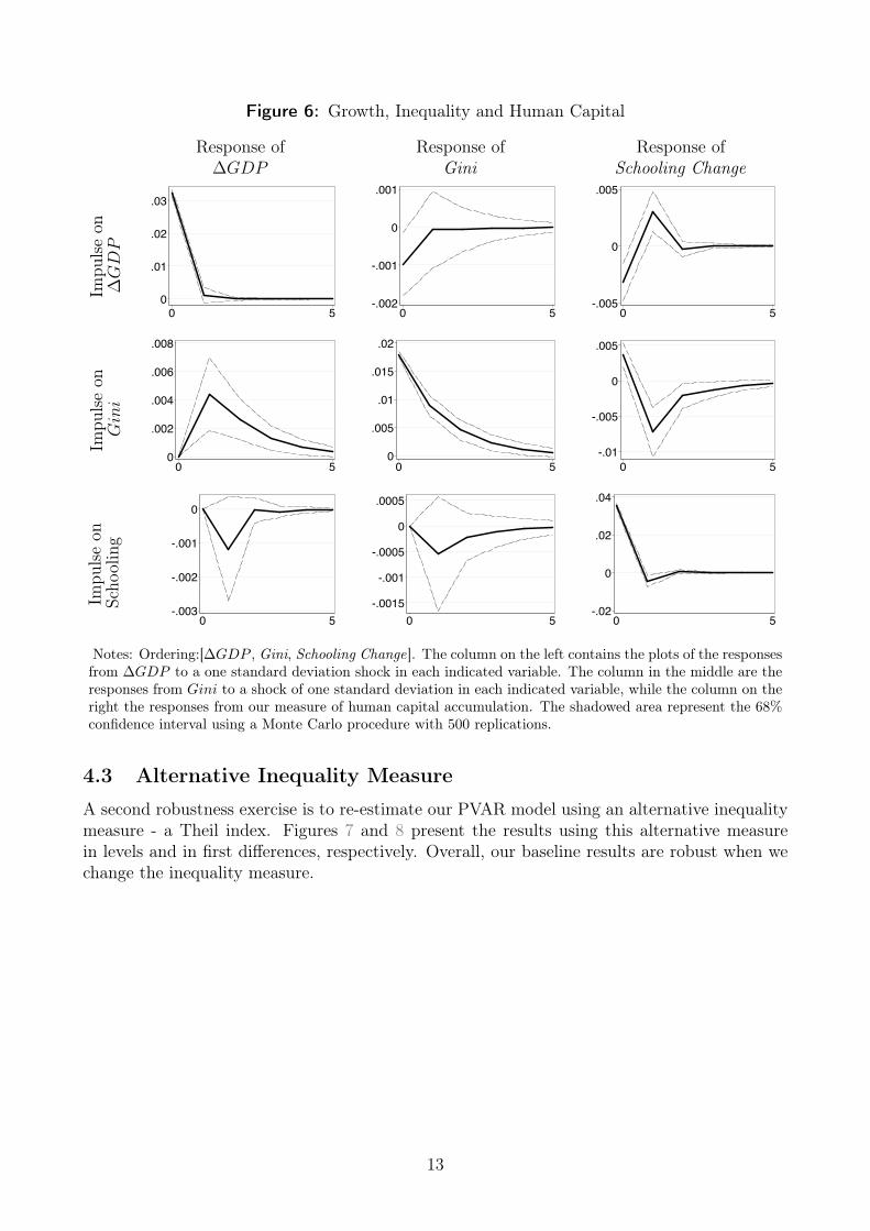
Figure 6: Growth, Inequality and Human Capital

Response of Response of Response of∆GDP Gini Schooling Change

Impu

lseon

∆GDP

0

.01

.02

.03

0 5-.002

-.001

0

.001

0 5-.005

0

.005

0 5

Impu

lseon

Gini

0

.002

.004

.006

.008

0 50

.005

.01

.015

.02

0 5-.01

-.005

0

.005

0 5

Impu

lseon

Scho

oling

-.003

-.002

-.001

0

0 5-.0015

-.001

-.0005

0

.0005

0 5-.02

0

.02

.04

0 5

Notes: Ordering:[∆GDP , Gini, Schooling Change]. The column on the left contains the plots of the responsesfrom ∆GDP to a one standard deviation shock in each indicated variable. The column in the middle are theresponses from Gini to a shock of one standard deviation in each indicated variable, while the column on theright the responses from our measure of human capital accumulation. The shadowed area represent the 68%confidence interval using a Monte Carlo procedure with 500 replications.

4.3 Alternative Inequality Measure

A second robustness exercise is to re-estimate our PVAR model using an alternative inequalitymeasure - a Theil index. Figures 7 and 8 present the results using this alternative measurein levels and in first differences, respectively. Overall, our baseline results are robust when wechange the inequality measure.

13

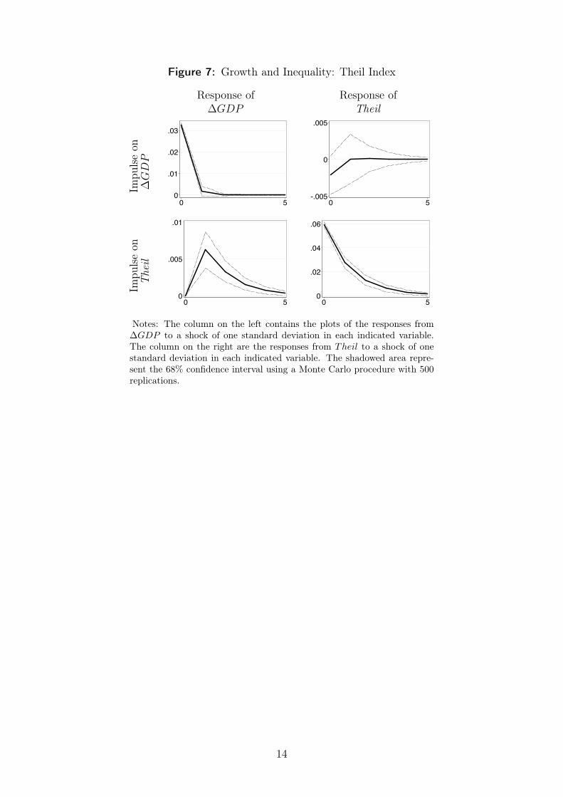
Figure 7: Growth and Inequality: Theil Index

Response of Response of∆GDP Theil

Impu

lseon

∆GDP

0

.01

.02

.03

0 5-.005

0

.005

0 5

Impu

lseon

The

il

0

.005

.01

0 50

.02

.04

.06

0 5

Notes: The column on the left contains the plots of the responses from∆GDP to a shock of one standard deviation in each indicated variable.The column on the right are the responses from Theil to a shock of onestandard deviation in each indicated variable. The shadowed area repre-sent the 68% confidence interval using a Monte Carlo procedure with 500replications.

14

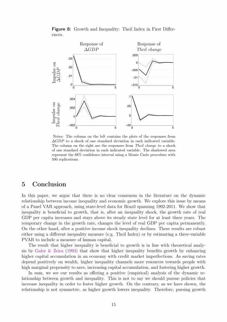
Figure 8: Growth and Inequality: Theil Index in First Differ-ences.

Response of Response of∆GDP Theil change

Impu

lseon

∆GDP

0

.01

.02

.03

0 5-.015

-.01

-.005

0

.005

0 5

Impu

lseon

The

ilch

ange

-.002

0

.002

.004

0 5-.05

0

.05

.1

0 5

Notes: The column on the left contains the plots of the responses from∆GDP to a shock of one standard deviation in each indicated variable.The column on the right are the responses from Theil change to a shockof one standard deviation in each indicated variable. The shadowed arearepresent the 68% confidence interval using a Monte Carlo procedure with500 replications.

5 Conclusion

In this paper, we argue that there is no clear consensus in the literature on the dynamicrelationship between income inequality and economic growth. We explore this issue by meansof a Panel VAR approach, using state-level data for Brazil spanning 1992-2011. We show thatinequality is beneficial to growth, that is, after an inequality shock, the growth rate of realGDP per capita increases and stays above its steady state level for at least three years. Thetemporary change in the growth rate, changes the level of real GDP per capita permanently.On the other hand, after a positive income shock inequality declines. These results are robusteither using a different inequality measure (e.g. Theil Index) or by estimating a three-variablePVAR to include a measure of human capital.

The result that higher inequality is beneficial to growth is in line with theoretical analy-sis by Galor & Zeira (1993) that show that higher inequality benefits growth by enhancinghigher capital accumulation in an economy with credit market imperfections. As saving ratesdepend positively on wealth, higher inequality channels more resources towards people withhigh marginal propensity to save, increasing capital accumulation, and fostering higher growth.

In sum, we see our results as offering a positive (empirical) analysis of the dynamic re-lationship between growth and inequality. This is not to say we should pursue policies thatincrease inequality in order to foster higher growth. On the contrary, as we have shown, therelationship is not symmetric, as higher growth lowers inequality. Therefore, pursing growth

15

enhancing policies should be translated not only in higher growth, but also in better incomedistribution.

16

ReferencesAbrigo, M. R., Love, I., et al. (2016). Estimation of panel vector autoregression in stata. Stata

Journal, 16 (3), 778–804.

Alesina, A. & Perotti, R. (1996). Income distribution, political instability, and investment.European economic review, 40 (6), 1203–1228.

Andrews, D. & Lu, B. (2001). Consistent model and moment selection procedures for gmmestimation with application to dynamic panel data models. Journal of Econometrics, 101 (1),123–164.

Arellano, M. & Bover, O. (1995). Another look at the instrumental variable estimation oferror-components models. Journal of econometrics, 68 (1), 29–51.

Atems, B. & Jones, J. (2015). Income inequality and economic growth: a panel var approach.Empirical Economics, 48 (4), 1541–1561.

Brueckner, M. & Lederman, D. (2015). Effects of income inequality on aggregate output. Policyresearch working paper; no. wps 7317, World Bank Group.

Brueckner, M., Norris, E., & Gradstein, M. (2015). National income and its distribution.Journal of Economic Growth, 20 (2), 149–175.

Cavalcanti, T. V. V. & Giannitsarou, C. (2016). Growth and human capital: A networkapproach. The Economic Journal, 1–39.

Forbes, K. J. (2000). A reassessment of the relationship between inequality and growth. Amer-ican economic review, 869–887.

Galor, O. (2011). Inequality, human capital formation, and the process of development. Hand-book of the Economics of Education, 4, 441.

Galor, O. & Moav, O. (2004). From physical to human capital accumulation: Inequality andthe process of development. The Review of Economic Studies, 71 (4), 1001–1026.

Galor, O. & Tsiddon, D. (1997). The distribution of human capital and economic growth.Journal of Economic Growth, 2 (1), 93–124.

Galor, O. & Zeira, J. (1993). Income distribution and macroeconomics. The Review of EconomicStudies, 60 (1), 35–52.

Li, H. & Zou, H.-f. (1998). Income inequality is not harmful for growth: theory and evidence.Review of development economics, 2 (3), 318–334.

Partridge, M. D. (1997). Is inequality harmful for growth? comment. The American EconomicReview, 87 (5), 1019–1032.

Persson, T. & Tabellini, G. (1994). Is inequality harmful for growth? The American EconomicReview, 600–621.

Pesaran, M. H. (2012). On the interpretation of panel unit root tests. Economics Letters,116 (3), 545–546.

17

Appendices

A Additional Figures

Figure 9: Roots of the compan-ion matrix

-1-.5

0.5

1Imaginary

-1 -.5 0 .5 1Real

18