NBER WORKING PAPER SERIES

DOES MARCH MADNESS LEAD TO IRRATIONAL EXUBERANCE IN THE NBADRAFT? HIGH-VALUE EMPLOYEE SELECTION DECISIONS AND DECISION-MAKING

BIAS

Casey IchniowskiAnne E. Preston

Working Paper 17928http://www.nber.org/papers/w17928

NATIONAL BUREAU OF ECONOMIC RESEARCH1050 Massachusetts Avenue

Cambridge, MA 02138March 2012

The authors thank Michael Egley, Damien Fenske-Corbiere, Kazunari Inoki, Amy Johnson, Jack Koehler,Raymond Lim, and Frankie Pavia for expert and dedicated research assistance on this project. Theyalso want to acknowledge Chaz Thomas and his dedication to his research on March Madness thatmotivated the current study. The views expressed herein are those of the authors and do not necessarilyreflect the views of the National Bureau of Economic Research.

NBER working papers are circulated for discussion and comment purposes. They have not been peer-reviewed or been subject to the review by the NBER Board of Directors that accompanies officialNBER publications.

© 2012 by Casey Ichniowski and Anne E. Preston. All rights reserved. Short sections of text, not toexceed two paragraphs, may be quoted without explicit permission provided that full credit, including© notice, is given to the source.

Does March Madness Lead to Irrational Exuberance in the NBA Draft? High-Value EmployeeSelection Decisions and Decision-Making BiasCasey Ichniowski and Anne E. PrestonNBER Working Paper No. 17928March 2012JEL No. J61

ABSTRACT

Using a detailed personally-assembled data set on the performance of collegiate and professional basketballplayers over the 1997-2010 period, we conduct a very direct test of two questions. Does performancein the NCAA “March Madness” college basketball tournament affect NBA teams’ draft decisions?If so, is this effect the result of decision making biases which overweight player performance in thesehigh-visibility college basketball games or rational judgments of how the players later perform in theNBA? The data provide very clear answers to these two questions. First, unexpected March Madnessperformance, in terms of unexpected team wins and unexpected player scoring, affects draft decisions.This result persists even when models control for a direct measure of the drafted players’ unobservedcounterfactual – various mock draft rankings of where the players were likely to be drafted just priorto any participation in the March Madness tournament. Second, NBA personnel who are making thesedraft decisions are certainly not irrationally overweighting this MM information. If anything, the unexpectedperformance in the March Madness tournament deserves more weight than it gets in the draft decisions.Finally, there is no evidence that players who played in the March Madness tournament comprisea pool of players with a lower variance in future NBA performance and who are therefore less likelyto become NBA superstars than are players who do not play in MM. Players with positive draft bumpsdue to unexpectedly good performance in the March Madness tournament are in fact more likely thanthose without bumps from March Madness participation to become one of the rare NBA superstarsin the league.

Casey IchniowskiGraduate School of Business3022 Broadway Street, 713 Uris HallColumbia UniversityNew York, NY 10027and NBERbei1@columbia.edu

Anne E. PrestonDepartment of Economics203 Stokes HallHaverford College Haverford, PA 19041apreston@haverford.edu

2 

 

I. Introduction

This paper examines the rationality of decision making of NBA scouts and executives by

addressing the question of whether a player’s performance in the NCAA “March Madness”

college championship basketball tournament unduly impacts how he fares in the NBA draft.

There are three possible answers to this question. Performance in the March Madness (MM)

tournament may provide no new independent information to NBA teams when they make their

draft day decisions and have no impact on NBA draft decisions. With half the MM tournament

teams only playing one game, and the average number of games per team approximately just two

games, this answer seems very plausible. Second, performance in the MM tournament may

impact NBA draft decisions in ways that lead the NBA teams to draft inferior players. While

scouts and executives have voluminous data on potential players they could draft, information on

performance in the high-profile MM tournament may receive undue weighting in their decision

making calculations. The expansive experimental literature on heuristics involved in decision

making under uncertainty suggests several reasons why this might in fact be the case. Finally, it

may be rational for NBA scouts and executives to pay special attention to performance in the

college championship tournament. Performance in this pressure-filled widely-watched

competition among the top teams in the country may offer a unique opportunity to learn about

how a college player will fare in the NBA.

To address this question and test which of these three answers is correct, we first model

whether performance in the NCAA March Madness tournament impacts draft position. For the

sample of college basketball seasons from 1997 to 2010, we examine the performance of players

and teams that qualified for the NCAA college championship tournament. We measure the

“unexpected” performance of each team in the tournament as the difference between expected

3 

 

wins given its tournament seeding and actual wins, and the “unexpected” performance of each

player as the difference between his season-long average performance and his performance in his

March Madness games. We then estimate models that test whether these measures of

unexpected team and player performance predict NBA teams’ draft decisions in a number of

different samples of potential draft picks. Second, we estimate the magnitude of any effects of

unexpectedly good or bad MM performance on each player’s draft outcomes, and thus the

difference between where a player was drafted and where he would have been drafted had he not

participated in the MM tournament. Third, any positive or negative MM-induced “bumps” in

draft position are then considered as potential predictors of several measures of the players’

future success in the NBA, including whether or not the player made an NBA team, games

played, standard performance measures like points or rebounds per game, and several advanced

performance metrics for both regular and post season games. To the extent that the MM

tournament does induce bumps in draft position, and that any such bumps change the accuracy of

the predictions that players are successful in the NBA, we offer information on whether NBA

teams are on average overemphasizing MM performance in their draft day decisions.

II. The NCAA March Madness Basketball Tournament and the NBA Draft

The NCAA Division 1 Basketball Championship Tournament

Division 1 of the National Collegiate Athletic Association (NCAA) now has 344

basketball teams. Each year, the winner of the end-of-season national championship tournament

in March is crowned the NCAA division 1 champion. During the 1997 to 2010 sample period for

this study, the field of college teams competing in this tournament was 64 teams through 2000,

4 

 

and 65 from 2001 when one play-in game was added through 2010.1 A selection committee

picks and seeds the teams. Teams that win their conferences, usually through a conference

tournament but occasionally through the regular season championships, receive automatic berths.

In today’s tournament with 68 teams, there are 31 automatic seeds and 37 at-large seeds.

Excluding the possibility that a team in a play-in game would win the tournament, the national

champion is the team that wins six consecutive games in this tournament in which a loss

eliminates a team.

The selection committee not only picks the at-large teams, but they also seed the teams.

These decisions are made based on team records, strength of team schedule, end-of-year

improvements or declines in team performance, number of wins against the very top teams in the

country, and more. There are four regional tournaments and the top four teams according to the

seeding committee receive the number one seeds in the four regions. Each region has teams

seeded 1 through 16, with a play-in game for one of the 16th seeds in the years the tournament

had 65 teams. Regional tournament winners play a semi-final game, with semi-final winners

meeting in the national championship game. The selection committee rankings have proven

accurate. The lowest seeded team to win the national tournament in our sample period was the

University of Arizona – a number four seed – in the 1997 tournament. Number 1 seeds are

commonly the tournament winner and no number 16 seed has ever won a tournament game. As

described below in the description of the data, the difference between a tournament team’s actual

wins and it’s expected wins given its seeding is an important measure of “unexpected success” in

the tournament.

                                                            1 The field expanded from 65 to 68 teams for the 2011 tournament with the addition of a “first four” set of play-in games rather than just one play-in game.

5 

 

The NBA Draft

The National Basketball Association (NBA) draft occurs each year usually in late June –

after the NBA league’s playoffs and championship series have concluded. While the NBA draft

has had as many as 19 rounds historically, it is a two round draft during the 1997-2010 sample

period. With 30 NBA teams, 60 players are selected.2 While our sample described below is

largely confined to players whose teams played in the NCAA tournament in a given year, drafted

players will also include college players on teams that did not qualify for the tournament, foreign

players not enrolled in U.S. colleges, and in many years in our sample period, high school

prodigies.

Current NBA draft rules state that all college seniors are automatically draft eligible, and

underclassmen can declare for the draft as “early entry” players in a written statement to the

NBA. The deadline for these applications is in late April, well after the NCAA tournament.

These same players can then withdraw from the NBA draft in a written statement received at

least 10 days prior to the draft which is held in late June. A player who has withdrawn from the

draft can return to college as long as he has not contacted an agent. Over the course of our

sample, the main change in draft eligibility occurs in the 2006 NBA draft when a minimum age

requirement of 19 was instituted for all drafted players as well as a requirement for US players to

be one year removed from their high school graduation. Prior to 2006, there was neither a

minimum age nor a post-high school time requirement of one year.

Since NBA rosters consist of only 12 active players with playing time largely given to a

rotation of the top 8 or 9 players on a team, NBA teams’ draft decisions are high value decisions

                                                            2 Until the 2004 draft, there were only 29 NBA teams before the Charlotte Bobcats were added as an expansion team. In some years, there is one less first round pick than second picks due to picks that were forfeited without replacement due to violations of the terms NBA’s collective bargaining agreement concerning salary caps. 

6 

 

with important impacts on the success of the team. For example, of all the first round draft picks

in the 1997 draft, the first year in this study’s sample, the minimum, average, and maximum

playing careers of the drafted players who made an NBA team were 15 games, 387 games, and

1053 games respectively. Making the most accurate prediction on a player’s future success is

clearly important.

III. Decision Making Bias and the NBA Draft

In deciding on draft picks, NBA teams are making high-stakes bets on the future

professional success of a collegiate player. A vast literature on the biases and heuristics that

people rely on when making decisions under uncertainty now exists, and ideas from this largely

experimental literature suggests a number of ways that performance in the collegiate MM

tournament might affect NBA decision makers. Some ideas from this literature suggest that NBA

scouts and executives may “irrationally overemphasize” information from the MM tournament

when they make their draft picks, while other ideas in this literature suggest that careful

deliberation will limit any such systematic irrational biases.

The Availability Heuristic

Some of the concepts in the research on decision making biases suggest that player and

team performance in the MM tournament may unduly, and irrationally, affect NBA draft

decisions. One category of decision making biases is referred to as the “availability heuristic.”

Under this heuristic, people judge the likelihood of an event – in the current study, the likelihood

that certain characteristics of a college player’s history and performance predict his future

success in the NBA -- by “the ease with which instances [of those characteristics] come to

mind.” (Kahneman, 2011, 129). Many studies on the nature of the availability bias indicate that

7 

 

characteristics that activate this bias by making it easier for confirming examples to come to

mind are when the prior examples are recent, vivid and dramatic, and personally observed and

experienced.

Each of these descriptions would seem to apply closely to the highly visible, much

watched, and extensively covered March Madness tournament. Perhaps most obvious,

information on performance in this tournament will be especially “available” because NBA

scouting of this tournament is very extensive due to the large number of top teams and players

involved. Performance in the tournament is also the most recent competitive basketball

experience for all college players before the draft, and it is a dramatic and vivid set of

experiences. Finally, the extent of exposure and coverage of this tournament far outpaces the

coverage of even the highest profile regular season games.3

Factors Limiting Decision-Making Biases: “Slow Thinking”

At the same time, decision making biases are most pronounced in spur of the moment

decisions. When people do not have to make quick decisions and instead have the time to

evaluate evidence analytically, thoughtful calculations and rational decision making come to the

fore. Kahneman (2011) summarizes decades of research that lead to a conclusion that decision

making biases, such as a reliance on the availability heuristic, commonly occur when we must

“think fast,” but when we have the chance to “think slow,” decision biases impact final decisions

much less. There are several months between the NCAA championship game and the NBA draft

with ample opportunities for the staffs of NBA teams to evaluate the wealth of data they have

                                                            3 In the 2011 NCAA tournament, telecasts averaged a 6.4 rating across all telecasted games, including four play-in games, or 10.2 million viewers on average. The largest regular season audience for a collegiate game in the same season occurred in the game between #9 Duke and #5 North Carolina which earned a 2.2 rating for approximately 3.1 million viewers. Visits to NCAA online and mobile platforms for the MM tournament total in the tens of millions and far outpace visits for regular season games. 

8 

 

collected on prospects including their physical and athletic abilities, interviews, historical data

and all game performance statistics and video evidence. Teams also conduct individual

workouts for a number of likely prospects in the time between the end of the MM tournament

and the NBA draft. Even if examples of performance from the MM tournament are relatively

more recent, dramatic, and impactful, NBA teams have ample opportunity to put the experiences

of heroes from Cinderella teams or goats from highly-ranked teams that lose first-round games in

the NCAA tournament into a fuller context when they are making these high value decisions.

There are of course hybrid versions of these competing ideas. For example, while the

typical cognitive mechanisms behind the availability heuristic – quick recall of the most easily

retrievable examples and evidence relevant for a decision – may not apply due to the time that

elapses between the NCAA tournament and the draft and to the high price tag and large

economic consequences of these picks, draft decisions remain highly uncertain. The NBA

decision makers may still convince themselves that dramatic clutch performances by players on

underdog teams in the MM tournament deserve to be weighted heavily when, in fact, the

memorable plays from the small sample of observations is no more revealing of ability than any

other game or two in the player’s history. Thus, the availability heuristic may still bias NBA

draft decisions despite the lengthy deliberations teams go through in making these decisions.

Conversely, NBA executives may pay attention to performance in the MM tournament

when they make their draft picks, not because of any heuristics or biases, but because it provides

truly unique and valuable insights about how draft prospects might fare in the NBA. There is

only one national collegiate championship, and unlike any other games in the year, a loss ends

the team’s season. For many teams from smaller conferences, the games are played in the largest

arenas they have ever played in with bigger in-person and television audiences than have

9 

 

watched any other games during the regular season, replicating the NBA game environment

better than most any other collegiate games. The level of competition is comprised of what an

expert panel believes to be the top teams in the country. Perhaps it is rational to weight

unexpectedly good or bad performance in the MM tournament as especially important. While

theoretical arguments can be marshaled on all sides of these questions, whether or not NBA

teams place significant weight on unexpected performances in the MM tournament and whether

any such MM-related changes in draft decisions reflect a rational weighting of this evidence are

ultimately empirical questions.4

Prior Studies of Professional Sports Draft Decisions

A number of studies have been conducted on factors that impact the draft decisions of

professional sports teams. Most studies do not explicitly invoke the idea of decision making

biases in professional sports draft decisions, but several studies do examine factors that predict

draft decisions and some also compare whether factors that predict draft pick order also predict

subsequent success as a professional. In studies that examine the impact of draft outcomes on

future success in a professional league, the most common question considered is whether earlier

draft picks have more success as a professional that later picks.

With regard to NBA draft decisions, the analysis by Thomas (2009), which motivates the

current study, finds a positive correlation between scoring more points and being on a team that

wins more MM games and being picked earlier in the draft during the 2004-2008 seasons. While

                                                            4 In the empirical work, we will judge the “rationality” of any change in draft rankings due to unexpected performance differences in the MM tournament by whether any such MM-induced changes in draft positions improve the predictions of future NBA career success. One could argue that it may be economically rational to pick a higher profile collegian, even if an NBA team is confident that a less well-known player will be a better NBA player, because such players would be bigger gate and television attractions. While we suspect that this mechanism would be at best very short-lived and dwarfed by the effects that more talented players would have on television and gate receipts from improving team winning percentages and numbers of appearances in NBA playoff games, we do acknowledge the limitation of the empirical work below that focuses on the players’ NBA game and career performances rather than on a direct measure of team profitability.

10 

 

this study does not consider how various NBA draft picks later fare in the NBA, Berri et. al.

(2011) examine a sample of college players between 1995 and 2009 to identify the

characteristics that determine draft position and whether the actual draft position predicts

performance in the NBA. In addition to the importance of points per NCAA game as a predictor

of draft position, they find that a final four appearance in the NCAA tournament is correlated

with an improvement in draft position of team members by 12 slots while winning the

championship is correlated with an improvement in draft position by another 8 slots. In this

study, the only other team-level variables in the draft order models are dummies for conference,

so the final four appearance and the national championship victory may be proxies for the quality

of the player’s college team, rather than the effect of new information gleaned from tournament

performance. They also find that the draft position is a significant determinant of subsequent

NBA career performance. Coates and Oguntimien (2008) present slightly conflicting results.

Examining players drafted between 1987 and 1989, they find that the effect of college scoring

(points per game) on draft position is insignificant while field goal and free throw percentages

also impact draft position. In predicting NBA performance, draft position and college scoring

help predict NBA scoring.

Some studies on draft decisions in other sports consider whether decision-making biases

may be affecting draft pick decisions. Massey and Thaler (2006) examine the NFL draft which

is similar to the NBA draft in that it chooses predominantly from college players. They argue

that managers overvalue high picks, both in terms of the salaries high picks receive and how

many lower draft choices are traded for higher draft picks, given the subsequent NFL

performance of the higher and lower draft picks. They interpret the evidence as suggestive of

systematic biases in decision making due to overconfidence and non-regressive predictions on

11 

 

the part of scouts and managers. Berri and Simmons (2009) also examine the NFL draft but

focus exclusively on quarterbacks. They find that the factors which predict draft selection order

of quarterbacks, particularly individual physical characteristics such as height, 40 yard dash time,

and score on the Wonderlic cognitive ability test, have little effect on NFL performance. They

conclude by questioning the ability of managers and scouts to evaluate these players whose

future performance is necessarily uncertain. Hendricks, DeBrock, and Koenker (2003) also focus

on the uncertainty of future performance of players drafted into the NFL. They show that teams

tend to use their early, more expensive, draft picks on college players from groups which send

out a more reliable signal of performance, i.e. division I college players. They use later picks to

choose from less reliable groups in hopes of getting a star.5

IV. Data Description: Samples and Variable Descriptions

The two main components of the empirical analysis are: first, estimates of the effects of

MM performance on position in the NBA draft; and second, estimates of the effects of any MM-

induced “bumps” in draft position on future NBA success. We create two data sets for the two

main portions of the empirical analysis. The first data set combines data on player and team

performance in regular season and MM college games during the 1997-2010 years with data on

NBA draft outcomes in those years. The second data set combines data on the performance of

the collegiate players in their NBA careers (if any) with the data on whether a given player had

been drafted, and if so, what his draft position was.

                                                            5 With respect to the NBA team’s decisions about playing time after draft picks have joined a team, Staw & Hoang (1995) and Camerer & Weber (1998) find evidence of a “sunk cost effect,” in which managers play earlier round draft picks more than is predicted by their performance statistics. They rule out rational explanations in favor of the idea that managers cannot separate their playing decisions from the large costs that they have put behind certain players, resulting in an escalation of commitment.

 

12 

 

Collegiate Players, Performance in College Games, and the NBA Draft

Sample. For this portion of the analysis, the maximum sample will have data on the top

five players, as measured by minutes per game in regular season games, from each college

basketball team that qualified for the NCAA tournament in each year between 1997 and 2000.

Because some of the elite NCAA teams have more than five potential NBA players on their

college rosters, we also augment this sample of five players per MM team to include data on all

players who were drafted or were identified as NBA prospects using the Heisler mock draft

(1997-2010), the NBA mock draft (2001-2010) or the Draft Express mock draft (2005-2010).

Across all 14 years and prospect surveys, thirty collegiate players in the sample, coming from 25

different teams, make up this category of NBA prospects who were not one of the top five

players in terms of minutes played per game on their college team. Therefore these 25 MM-

qualifying teams have more than five players included in the analysis of MM performance and

draft decisions. The effects of MM performance on draft outcomes are also examined in a

number of more restrictive subsamples.

Dependent Variable: NBA Draft Outcomes. For all players drafted in the 1997-2010

draft, whether the players played in the MM tournament or not, we have information on draft

number (if drafted), and draft number in mock drafts. Merging this information with the sample

of players who played on MM teams in each year between 1997 and 2010 allows us to identify

whether collegiate players with different levels of performance in the MM tournament were

drafted high, low, or not at all. (Sources for all variables described in this section are reported in

the Data Appendix Table.)

Mock Draft Outcomes. An important feature of the empirical analyses, as described

further in the model section below, is that the close scrutiny that professional sports receives

13 

 

offers a unique and separate measure of the unobserved counterfactual. In this part of the

empirical analysis, the unobserved counterfactual is where the various players would have been

drafted had they not played in the MM tournament. We have collected data from three separate

sources on “mock drafts” that were published just prior to the MM tournament. In models that

include this information, we often rely on the Heisler mock draft since it is the one mock draft

covering the entire 1997-2010 period.

The main drawback of the Heisler mock draft is that it is a first round mock draft and

covers only 30 players (or 29 prior to NBA expansion in the sample period). Because of this

limitation, and because of the importance of the mock draft information in making the empirical

tests of the effects of MM performance on NBA draft day outcomes more convincing, we also

collected data on pre-MM mock drafts available from NBA.com and Draftexpress.com. The

NBA.com mock draft covers years from 2001 to 2010 and is a two-round mock NBA draft. The

draftexpress.com mock draft is a two-round mock draft covering only the years since 2004.

Models of actual NBA draft day outcomes that control for mock draft positions consider each of

the mock drafts as predictors of draft outcomes to test whether any estimated effects of MM

performance on draft outcomes is sensitive to the choice of which mock draft is used as a

control.

Characteristics of MM Players and Teams. For each player in this sample, we collect

information on height, weight, age, college class, and position. We also collect statistics on

games played, points, rebounds, assists, steals, blocks and turnovers, for the players’ full seasons

prior to any MM games. For ease of reference, we refer to these season-long statistics that

exclude performance in MM games, as the players’ “regular season” statistics, even though for

many of these players, these “regular season” statistics also include data on performance in

14 

 

conference tournament games. Finally, for this analysis, we also assemble MM tournament

statistics on these same performance measures as well as each team’s tournament seeding and its

actual record in the tournament.

Unexpected Team and Player Performance in the MM Tournament. Of principal interest

in the first stage of our empirical analysis is whether performance in the MM tournament impacts

the dependent variable measuring NBA draft outcomes. MM tournament performance should

only affect draft position if it is unexpected, and we measure “unexpected MM performance” at

both the team and player levels.

Expected team performance is determined by the seeding of the team. As described in

Section II, seeds range from 1 to 16 in each of four regions as determined after deliberations and

analyses by the seeding committee of the NCAA. To measure unexpected team performance, we

create a variable, PASE, or a given team’s performance against seed expectations, which is the

difference between actual wins and expected wins. Expected wins are generated empirically

based on historical performance of seeded teams; e.g., how many games have teams ranked 16 or

15 etc. won in the NCAA tournament since the time the tournament has had a format of 64 or 65

games. In addition, we have collected individual player performance measures for the MM

tournament games. We create “unexpected” individual performance statistics by subtracting per

game performance measures for the regular season from the same statistics for the tournament.

NBA Game and Career Performance

The second part of this study’s empirical analysis builds on the first. Once we test for

any effects of unexpectedly good or bad MM performance on NBA draft outcomes and measure

any MM-induced bumps in the draft outcomes, we test whether those bumps in draft order end

15 

 

up, on average, improving or harming the accuracy of the draft order’s prediction on future NBA

success. This second-stage analysis requires data on players’ performance in the NBA.

Sample. The sample for the analysis in this second stage includes all players who were

drafted in the NBA draft between 1997 and 2010 and any player who began their NBA careers in

these same years, even if they had not been selected in the draft. Most models in the second part

of the empirical analyses only examine this sample of NBA players, sometimes restricting the

sample to only drafted players or to only drafted players who played in MM. In certain analyses

that examine which players ever made an NBA team, we also expand the sample to include

various groups of collegiate players from the first-stage analysis who never made the NBA,

either because the collegiate player was drafted (in the second round of the NBA draft) but never

made an NBA team, or because he was a former MM participant who was never drafted and

never made the NBA. For these players, all NBA statistics (such as games played) will be zero or

missing. This sample will allow us to compare the NBA careers (if any) of players who were

drafted early in the draft to those who were drafted later in the draft to those who were not

drafted. The effects of MM-induced bumps in draft status on future NBA career success during

the 1997-2010 period will be the central focus on this analysis.

Dependent Variables: NBA performance. For all players who joined the NBA in this

time period, we collected measures of performance in the NBA. We have both career and yearly

performance statistics that cover traditional performance statistics, such as games played, points

per game, assists, rebounds, and the like, as well as several “advanced” statistics on offensive

and defensive performance on regular and post season play. Some drafted players and many MM

participants do not make an NBA team, and when these collegiate players are included in the

analyses, the number of NBA games ever played will be zero.

16 

 

Descriptive Statistics: Collegiate Performance of Drafted and Undrafted Players

Table 1 gives personal and collegiate performance statistics on all collegiate players who

played in the NCAA tournament between 1997 and 2010 and the subsets of drafted and

undrafted players. According to the first column, on average, these players played roughly 30

games in their season (not including any MM games), and 29 minutes per regular season game.

9.3 percent of this sample of MM participants was drafted. However, as described above in

Section II, while all MM participants could theoretically become eligible for the NBA draft, not

all of these players are eligible at the time of the NBA draft since most underclassmen do not

declare for early entry. In these years, 33.0 percent of the players in this sample of NCAA-

tournament participants were eligible for the draft because they were seniors or because they

were underclassmen who had declared for the draft in accordance with the CBA’s rules for the

given season. 5.2 percent of the sample are early entrants in their given draft year. As expected, a

very high percent of all early entrants (86%) are in fact drafted, since no player would declare for

the draft early unless he believed he would be drafted.

A comparison of the performance statistics in columns 2 and 3 reveals that drafted

players’ performance statistics are superior to the statistics for undrafted players. These

differences in performance measures between drafted and undrafted players in lines 7-13 of

Table 1 are all significant at the 0.01 level.

--------------- Table 1 here ---------------

Table 2 reports descriptive statistics on the various team- and player-level measures of

“unexpected MM performance.” The average value of the team-level performance against

seed’s expectation, PASE, for the full sample is essentially zero, as expected. The two largest

17 

 

positive value of PASE in the sample exceed four games: 4.48 unexpected wins for National

Champion Arizona in 1997 (seeded 4th), and 4.21 unexpected wins for National Champion

Syracuse in 2003 (seeded 3rd). The largest negative value for PASE in the sample is -2.43 games

for Iowa State in 2001 (seeded 2nd). Also shown in column 1, average values for all player-level

statistics that measure the difference in performance between regular season games and the MM

tournament are negative. Players’ performance statistics on average decline from the regular

season to the tournament, again as one would expect, since the average level of competition is

higher in the tournament than in the regular season.

--------------- Table 2 here ---------------

A comparison of columns 2 and 3 of Table 2 reveals that drafted players have

significantly higher PASE than non-drafted players. A drafted player who participated in the

MM tournament, on average, comes from an MM team that did better than their seed would have

predicted. Drafted players still have on average fewer points, assists, steals, and blocks as well

as higher turnovers in the tournament than in the regular seasons. However, with respect to

points, assists, and rebounds, the reductions that drafted players experience in going from regular

season games to MM games are significantly smaller than the reductions observed for the non-

drafted players. Drafted players are doing relatively better in the tournament, in terms of

relatively smaller drop offs in key performance statistics from the regular season to the MM

tournament, than non-drafted players.

18 

 

V. Modeling the Effect of Unexpected MM Performance on NBA Draft Position

Assume that player quality is represented by a latent unmeasured player quality variable

*iQ where iiiii NPXQ

* . iX

is a vector of individual characteristics including

height, weight, class, position, and conference of team. iP

is a vector of individual performance

measures for the regular season including number of regular season games played, per game

averages of points, rebounds, assists, steals, blocks and turnovers, and the team’s March

Madness seed, a general indicator of team performance and quality in the regular season. iN

is a

vector of team- and player-level variables measuring unexpected performance in the NCAA

tournament, and i is a normally distributed error term with mean zero and variance 2 . We do

not observe the latent variable, *iQ , but a censored proxy iQ , the draft position of the player.

Some players with MM game experience are drafted high, some low, and most not at all.

Therefore, one can represent the analysis of the determinants of this inverted draft order variable

as a two-limit tobit estimation:

iQ = 0 if *iQ LL

iiiii NPXQ

if LL > *iQ < UL

iQ = 60 if *iQ UL

LL represents the lower bound below which a player will not be drafted and UL represents the

upper bound, above which the player will be drafted first.

In most tobit models we estimate, the dependent variable is the inverted draft order with

the top pick receiving a value of 60, the second pick 59, and so on, down to the last pick which

19 

 

receives a 1. Values of zero are assigned to all undrafted players.6 The independent variables of

principal interest are the MM performance variables in the vector iN

. As described in Section

III, it is “unexpected” performance in the MM tournament that might lead MM performance to

impact draft position. We include PASE, team performance against seed expectations, in iN

.

We also include the differences between tournament performance statistics and the

corresponding statistic for the player’s regular season games, for example, the difference

between average points per game in the MM tournament and in regular season games.

VI. Empirical Results on the Effects of MM Performance on NBA Draft Outcomes

We estimate tobit models described in Section V to examine the effects of unexpectedly

good or bad performance in the MM tournament on the inverted draft position variable, where 60

is the value for the first player selected (and at the upper limit of the tobit), 1 is the value of the

dependent variable for the last player selected, and players who are not selected receiving a value

of zero (and below the lower limit of the tobit). Control variables are those described in the

preceding section including measures of players’ regular season performance and team quality

measures. The models also include year fixed effects to allow the pool of players to have more

or less talented players in the different years. The key variables of interest are ones that test

whether NBA teams pay attention to differentially good or bad performance in the MM

tournament – the team-level PASE variable and the vector of variables measuring the difference

                                                            6 Because higher quality individuals earn a lower (earlier) draft position, we suspect confusion in interpretation of the empirical results might arise and therefore reverse draft position numbers so that earlier (later) draft picks are assigned higher (lower) values for the dependent draft order variable. Thus, variables in these tobit models that have positive coefficients will be variables that predict the more highly rated and valued players.  

20 

 

between a player’s MM performance (points, rebounds, assists, steals, blocks and turnovers) and

his regular season performance.

Broad Samples of Collegians versus Highly Selective Samples of Top NBA Prospects

In the empirical analyses of determinants of the NBA draft outcomes to follow, we

estimate the effects of MM performance and other variables in both very large samples of

collegiate players and much more restricted samples of only the top NBA prospects. Draft order

models estimated in the two types of samples address somewhat different questions given the

different degrees of selectivity imposed on the samples. In the broadest samples, most of the

college players truly have no chance of ever being among the top 60 players drafted; while in the

more narrowly defined samples of potential top draft picks, some or all players get drafted. This

study may well be one setting where the impact of practical interest is the impact of the various

MM performance variables in the more selective samples. For example, unexpectedly strong

performance by the third or fourth best player on a 16th-ranked MM team may substantially

improve an NBA scout’s opinion of that player, but the evaluation of that player will still fall

well below the talent levels of the pool of NBA draftees. Still, with the broader samples, the

tobit models attempt to estimate the effect of the independent variables across a broad range of

talent levels. We begin our analyses by estimating the effects of variables measuring unexpected

MM performance on the broadest possible sample of collegiate players that we have collected

and then replicate the models for more and more selective samples of the most talented

basketball players, eventually estimating the impact of the MM performance variables on

potential top 10 NBA draft picks.

Full MM Sample Estimates

21 

 

Table 3 reports results for different specifications of the tobit model for the broadest

possible sample of college players in our data – those collegiate players on MM teams who had

the top five values for their team on minutes played per game, plus for a few teams, additional

players if other players had been identified as NBA prospects in the various NBA draft ranking

websites described in the data section above. While many of these players are not in any way

serious NBA prospects, they are all theoretically candidates for the draft but simply fall too far

below the cutoff of the Q* talent variable to be drafted. Such a sample that examines close to the

universe of MM players (or at least those with large amounts of MM playing time) imposes the

least selectivity on the players being considered, and therefore attempts to estimate the effects of

the various MM performance variables among typical players on strong collegiate teams. For

example, a player may in some sense receive a positive “bump” in the eyes of NBA scouts

watching his MM games, but that bump can still leave the player well below the level for any

consideration of being drafted by an NBA team.

--------------- Table 3 here ---------------

The tobit model in column 1 of Table 3 only includes PASE to describe team-level

unexpected performance, and is estimated for this broad sample of 4,335 MM participants. The

estimated coefficient is 5.6 and significant at the 0.01 level. The estimated marginal effect of a

one game change in PASE, when the marginal effect is estimated for uncensored observations at

the mean of the independent variables, is .504 draft spots.7 The standard deviation of PASE is

                                                            7 Throughout this section, we translate estimated tobit coefficients into the marginal effects among uncensored observations. Essentially we are looking at the change in the mean of the draft position conditional on latent quality

22 

 

1.015 so 0.5045 is also the expected change in draft order from a one standard deviation change

in PASE. In the column 2 model, we allow for separate effects of positive values of PASE

versus negative values of PASE to determine whether unexpected good performance has a

different impact on draft position than unexpected bad performance. Both the PASE positive

(row2) and the PASE negative (row 3) variables have significant coefficients with similar

magnitudes (within 0.013 of each other), and an F test reveals that we cannot reject the

hypothesis that the two coefficients are equal. Therefore subsequent models do not separate the

effects of the PASE variable into the effects of PASE when it is positive versus negative.

Because PASE is a team-level variable, the estimated model is constraining the effect of PASE

to be the same for all players on the team. It may well be that the effect of PASE may vary

across more and less talented players. Rather than interact PASE with player-specific measures

of talent in the models here in Table 3, this issue is addressed in later models when we estimate

similar models to the ones in Table 3 but for more and more selective samples.

In column 3 we add the player-level measures of unexpectedly good or bad performance,

the difference between the average points (rebounds, assists, steals, blocks, and turnovers) per

MM game and the average points (rebounds, assists, steals, blocks, and turnovers) per regular

season game (rows 4-9) The difference in points (row 4) and the difference in assists (row 6)

are both significant at the .10-level. The coefficient on PASE remains essentially unchanged.

                                                                                                                                                                                                being above the lower limit and below the upper limit. The marginal is given by:

2

*

)(

)(

)(

)(1

0,|[

i

i

i

i

ik

k

iii

X

X

X

XX

X

QXQE

The extent to which the marginal effect will be less than the estimated coefficient βk, depends on the value of the estimated variance and mean of draft position at which we are evaluating the marginal, and these values differ across the different samples. Thus, the magnitude of the tobit coefficients on a given variable across different samples does not immediately indicate differences in the magnitudes of marginal effects among uncensored observations.

23 

 

According to these results, team-level and certain individual-level measures of unexpected MM

performance impact draft outcomes.

Finally, the estimates from the tobit models in columns 4-6 reveal that the effects of

variables measuring a player’s unexpected MM performance are concentrated among players on

certain teams. In particular, the tobit models in columns 4 and 5 display estimated coefficients

when the same model is estimated for the samples of players on MM teams that had better than

expected MM performance (PASE is positive, in column 4) and those players on MM teams that

had worse than expected MM performance (PASE is negative, in column 5). The column 6

model displays similar results, and shows coefficients for interaction variables that measure

player-level unexpected MM performance separately for positive PASE teams and negative

PASE teams.

In both the column 4-5 models for the PASE positive and PASE negative subsamples and

in the column 6 model with interaction terms between the unexpected player performance

variables and the PASE positive vs. negative dummy, the results show a similar pattern. Players

whose team has a negative PASE will not get further penalized (or helped) by their personal

performance. Players whose teams do better than expected are helped (or hurt) by personal

performance that deviates from their regular season level. One very plausible explanation for

this pattern is that when PASE is negative, NBA scouts are usually getting data on players in

only one or two games. When PASE is positive, and a team is on a run of wins, the performance

differences are being sustained over a larger sample of highly competitive games. Further the

hype following the surprising team often transfers to its players who are having a great (better

than expected) tournament. In all of these models, the coefficient on the team-level PASE

variable remains positive and significant.

24 

 

The effects of the player-level MM performance variables playing on teams that had a

positive PASE are effects above and beyond the effects of the team-level PASE variable.

Among PASE positive teams, the mean for the ∆ in Points variable is -.106 with a standard

deviation of 3.713. The coefficient on this variable among PASE positive teams from the

column 6 specification implies a marginal effect of .09 draft spots for a one point change, and .33

draft spots for a one standard deviation change in player points. Among PASE positive teams,

the mean for the ∆ in Assists variable is -.155 with a standard deviation of 1.071. The coefficient

on this variable among PASE positive teams from the column 6 specification implies a marginal

effect of .39 draft spots for a one assist change, and .42 draft spots for a one standard deviation

change in player assists. The estimated marginal impact of a one game increase (or decrease) in

the PASE variable shown in line 1 of table 6 is .481 draft spots. Thus, the estimates in the

column 6 model imply that a player, whose MM team wins one more game than expected and

who helps win the game with 4 more points and one more assist in the MM tournament than in

his typical regular season game, will improve his draft position by about 1.2 spots.

Controls for the Unobserved Counterfactual: Mock Drafts Prior to MM

The Table 3 results suggest that both unexpected team and individual performance impact

the draft position of players who participate in the NCAA MM tournament. The significant

effects of the team-level PASE variable and the player-level variables of unexpected points and

assists imply that unexpectedly good (bad) performance in the MM tournament gives a MM

participant a positive (negative) bump in his draft outcome. The preceding Table 3 models

generate their estimates of where a player would have been taken without their MM participation

from a wide array of control variables for the players’ physical characteristics, regular season

performance statistics, and measures of the quality of the team and collegiate conference. While

25 

 

these controls are extensive, omitted measures of player talent correlated with the MM variables

and draft outcomes will bias the estimated coefficients on the MM variables. Opportunities for

player fixed effects models do not exist in this setting because a player is only eligible for the

draft in one year. However, unique to this setting, there exist singular measures of the

unobserved counterfactual of where the player would have been drafted had he not played in

MM – mock draft rankings conducted just prior to the MM tournament. Because the mock drafts

are published just before the MM tournament, and because the time from the start of the MM

tournament to the NBA draft is roughly three months, we expect this ranking to be a uniquely

accurate control for omitted variables and the actual unobserved counterfactual.

In Table 4, we re-estimate the Table 3 column 6 model but include pre-MM mock draft

rankings as additional predictors of actual NBA draft outcomes. Column 1 reproduces the Table

3 column 6 model for comparison. In column 2, we enter the Heisler mock draft value as a

control. This is the one pre-MM mock draft that covers the entire 1997-2010 period (though it

only predicts the 29 to 30 draft choices since it is a one-round mock draft). We consider other

pre-MM drafts as controls in columns 3 and 4 as robustness checks to make sure estimates in

these models are not affected by possible differences in the accuracy of different mock drafts. In

column 3, we include the NBA.com mock draft values as a control. This mock draft is only

available since 2001, but has the advantage of predicting two rounds of draft picks. Finally, the

column 4 model includes an alternative two-round pre-MM mock draft from Draftexpress.com,

which is only available for the last six of the fourteen seasons in the MM sample of years.8

                                                            8 Mock draft values exist for only a small portion of all college players in our sample since they are predictions of who will be the top 30 (Heisler) or top 60 (NBA mock draft and Draftexpress) players drafted, and some of those predicted will be foreign players, high school players for some years, or collegians who did not play in the MM tournament. Mock draft rankings are inverted (eg, in the NBA mock draft control, the first pick receives a value of

26 

 

--------------- Table 4 here ---------------

The results in Table 4 show a very consistent pattern, despite any differences in which

mock draft is used as a control or differences in the years that are included in the sample.

Focusing on the column 2 model where the sample is identical to the column 1 model (because

the Heisler mock draft covers the entire 1997-2010 sample period), one observes that as expected

the coefficient on the Heisler rank (row 15) is positive and significant and close to 1.0. Higher

ranked players in the pre-MM mock draft are significantly more likely to be taken earlier in the

draft. However, the inclusion of the Heisler rank variable has minimal impact on the estimated

effects of the unexpected MM performance variables. The effect of PASE (row 1) declines

slightly as the marginal impact of a one game difference in PASE is .481 draft slots in the

column 1 model and .421 draft slots in the column 2 model. The coefficients on unexpected

points (row 2) and assists (row 4) interacted with PASE positive also remain significant in the

column 2 model that includes the Hesiler mock draft controls, with slightly larger estimated

effects on the points variable in the column 2 model relative to column 1, and slightly smaller

effects of the assists variable in the column 2 model. The coefficients on the personal

performance statistics interacted with the PASE negative variable continue to be insignificant.

With regard to the magnitude of these effects, a player who scores 4 more points with 1 more

assist than expected in MM and who plays for a team with one more MM win than expected is

predicted to move up in the NBA draft by 1.23 slots in the column 1model and 1.10 slots in the

column 2 model, with the slight reduction in change in draft spots in column 2 due largely to a

reduction in the size of the marginal effect of the team-level PASE variable.

                                                                                                                                                                                                60 and unranked players receive a value of zero). In each model we include a dummy variable equal to one for players not included in the given mock draft. 

27 

 

The samples in columns 3 and especially column 4 are smaller than the sample for the

column 1 and 2 models as these models are estimated for fewer years. This complicates the

comparison of the magnitudes of coefficients across models somewhat;9 however, the basic

patterns remain. Mock rankings (row 17 in column 3 and row 19 in column 4) are highly

significant predictors of actual draft outcomes. In column 3, PASE (row 1), and unexpected

points (row 2) and unexpected assists (row 4) among players on PASE positive teams again are

significant predictors of NBA draft outcomes. In the column 4 model which considers only the

six draft years for which the Draftexpress.com mock draft is available, PASE remains a

significant predictor of the draft outcomes. The significance levels of the effects of unexpected

points and assists interacted with PASE positive fall to the 0.15 level and the 0.16 level in the

column 4 sample for the 2005-2010 period.

Samples of Draft Eligible Players and NBA Prospects All of the players in this sample of MM participants are theoretically eligible for the

NBA draft, either because they are seniors or because they could declare for the draft. Of course,

most of these players have no chance of being drafted, and these unlikely-to-be-drafted players

comprise the large number of observations in the Table 3 sample for whom the dependent

variable is truncated below the lower limit in the tobit model. While it is valuable to examine

estimates of the effects of the MM performance variables in this broad sample with relatively

limited selectivity on the college players considered, one also would like to know how the

unexpected March Madness performance variables impact draft order within much more

selective samples, including samples of only the top prospects. For example, if you really are

talented enough to be under consideration by NBA teams as one of the 60 draft picks, will your                                                             9 See note 6 supra for the formula relating marginal effects among uncensored observations to estimated tobit coefficients.

28 

 

March Madness performance matter? Will unexpectedly good (poor) MM performance move a

top 10 NBA prospect up (down) in the actual draft? Do the estimates of the effects of MM

variables continue to be significant effects on draft order when we exclude less talented players

from consideration in the sample? Models in the next two tables consider increasingly selective

samples of collegiate players, moving from samples of only the players who were draft eligible

on the day of the draft to samples of only the very top NBA prospects.

The first column of Table 5 reproduces the Table 4 column 2 model (with a sample of all

MM participants in a tobit model that includes a control for the Heisler mock draft) for

comparison. The tobit models in subsequent columns then consider increasingly more restrictive

samples of draft eligible players. Column 2 of Table 5 replicates the column 1 model but only

for the sample of MM players who were actually eligible on the day of the NBA draft. This

sample includes seniors and declared underclassmen; but unlike the column 1 sample, it omits

underclassmen who did not declare for the draft. Columns 3 and 4 separate the column 2 sample

into samples of seniors (column 3) and the much smaller sample of declared underclassmen

(column 4).

--------------- Table 5 here ---------------

 

In all three models, PASE (row 1) remains positive and significant, as do the player-level

points (row 2) and assists (row 4) variables among players on teams with a positive value of

PASE. The lone exception to this pattern is an insignificant coefficient on the assists variables

for positive PASE teams in the column 4 sample of 232 early draft entrants. Other player-level

MM performance metrics continue to have insignificant effects with the exceptions of the

positive effect of unexpected MM blocked shots for PASE positive teams (row 6) and the

29 

 

negative effect of unexpected MM rebounds among PASE positive teams in the seniors sample

(row 3), and the negative effect of unexpected steals among PASE positive teams (row 5) in the

early entrants sample.

Because of the changes in the samples and changes in the mean draft ranking of the

uncensored players in these different subsamples, the relative values of the estimated tobit

coefficients do not directly indicate the relative size of the marginal effects of these variables

given the non-linear estimation method. A player whose team wins one more MM game than

expected and who scores 4 more points with one more assist than expected increases their draft

outcome by: 1.1 slots, 2.1 slots, 1.8 slots, and a very large 5.1 slots10 in the column 1 through 4

models respectively. Note too, that in the column 4 model (as in the tobit models to follow

estimated on samples of true NBA prospects), the effect of PASE essentially becomes an

individual-level effect rather than a team effect since there is typically only one such early

entrant (or prospect in later models) per team. While the estimated marginal effect of MM

performance measures on actual draft outcomes is relatively large among the sample of early

entrants, MM performance should be especially important for this group of younger players who

may have as little as one season’s worth of NCAA game experience before their MM

participation.11

In column 5 of Table 5, we report tobit model estimates for our first sample that consists

exclusively of true “NBA prospects.” In the column 5 sample, we define prospects to be any

                                                            10 This estimate includes the marginal effect of a one assist increase for a PASE positive team member even though the point estimate on the tobit coefficient in this model (-1.152) is insignificantly different from zero. 11 We also estimate a Heckman model for underclassmen where the first stage explains the decision to declare for the draft and the second stage explains draft order. In these models we use the number of seniors in the top 5 players on the current team and the number of years in the last five that the team has been in March Madness to identify the first stage equation (under the assumptions that teams with a lot of seniors will not be as successful next year while they are rebuilding, or will generally offer less of a showcase for a player’s talent). The results for draft rank look similar to the tobit of column 4, however the coefficients on PASE and the interaction of PASE positive and points are smaller in magnitude since these variables are also influencing the decision to declare.  

30 

 

player who was ranked in either the Heisler, NBA.com or Draftexpress mock drafts. The model

in column 5 controls for the mock draft rank.12 Unlike the previous models in Table 5 (and

those in Table 4), all players in this model’s sample have a mock ranking and thus there is no

dummy variable for “no mock ranking” included.

In the column 5 model for this sample of prospects for the years 1997-2010, the

coefficients on unexpected MM team wins (row 1) and unexpected MM points scored for both

PASE positive (row 2) and PASE negative (row 8) teams are significant and positive. Again,

note that the effect of the PASE variable in samples of prospects is now an individual player

effect since there is rarely more than one player per team in this sample, whereas in prior

samples the PASE effect applied to five or more players per team. The results in this column’s

model suggest that NBA teams are valuing players who help their teams win games that the team

was not expected to win. The marginal effects of a one game increase in PASE, a one point

increase above regular season point average for players on PASE positive teams, and a one point

increase above regular season point average for players on PASE negative teams are

respectively: 1.96 slots, .68 slots, and .34 slots. A one game increase in PASE and a one

standard deviation increase in unexpected points and assists corresponds to a change in predicted

draft order of approximately 5 full spots in the column 5 sample of NBA prospects.

Samples Only with NBA Draft Prospects

Table 6 reports additional models that continue to focus on NBA prospects only. Column

1 replicates the estimates from the Table 5 column 5 model for comparison, where the sample is                                                             12 The mock draft control in this model uses the NBA.com value if the NBA mock draft ranked the player, then the Heisler where this mock draft ranks a player but NBA.com does not, and then finally the Draftexpress ranking if this mock draft is the only one to rank the player. This rule for creating the sample of prospects in the column 5 model gives us the broadest possible definition of true NBA draft prospects. There is some inconsistency across years especially in the fact that for 1997-1999 we only have first round draft prospects as defined by Heisler. Table 6 examines a number of other definitions of prospects where the inclusion criteria are consistent across all years in the various samples.

31 

 

defined using the broadest possible definition of NBA prospects. Column 2 uses only the Heisler

mock draft to identify the sample of prospects. One can consider this to be a sample across all of

the years from 1997 to 2010 of potential first round draft picks (who also played in the MM

tournament). Column 3 uses the NBA.com mock draft to identify prospects, a pool of potential

first or second round draft picks, but only for the years 2000 to 2010.

--------------- Table 6 here ---------------

 

In all of the models in columns 1 through 3, PASE and unexpected points among PASE

positive teams are significant determinants of the NBA’s draft day outcomes. The positive

significant effects of unexpected MM assists among PASE positive teams estimated in the

broadest possible samples in Tables 3 and 4 are no longer observed among these samples of true

NBA draft prospects. Unexpected MM performance in terms of steals is found to be a

significant determinant of draft outcomes among the pool of potential first and second round

draft picks considered in the column 3 specification.

Across all models in Tables 3 through 6, two consistent results emerge – unexpected MM

wins and unexpected MM points, especially on teams with unexpected MM wins, impact NBA

teams’ draft decisions. The significant effect of PASE in the more restrictive samples of

prospects (for which the PASE effect typically applies to only one player team), combined with

the significant effect of unexpected MM points scored by prospects on those teams suggests the

following conclusion documented in all models in all tables. A prospect who scores more points

in MM games than one would have expected given his regular season scoring average and who

helps his team unexpectedly win MM games moves up significantly in the NBA draft. The

calculated marginal effects of having one more win than expected, together with 4 more points

32 

 

on a PASE positive team, in the column 1 through 3 models and samples are, respectively: 4.7

slots, 2.8 slots, and 5.0 slots.

Finally, does unexpected MM performance change the draft prospects of potential top ten

NBA draft picks? The model in column 4 of Table 6 addresses this question by restricting the

sample for consideration to those players among our set of MM participants who were also

ranked in positions 1 though 15 in the Heisler pre-MM mock draft. This is an especially

selective sample with some of the most talented collegians in each of the fourteen years we

consider, and is therefore the smallest sample considered in any of the tobit models estimated

thus far (N=115 MM participants). The mock draft ranking is, as expected, a significant

determinant of draft order. Players predicted to go earlier in the draft in a March mock draft are

still selected earlier in the actual NBA draft in June. The PASE variable in this smaller sample

of especially elite NBA prospects will again be an effect applying, almost without exception

across the 14 years in the sample, to only one player per team. In this highly selective sample,

PASE is no longer significant. However, unexpected MM points do matter for both players on

PASE positive teams (row 2) and players on PASE negative teams (row 8). Coefficients on

unexpected increases in assists (row10) and unexpected increases in turnovers (row 13) are

significantly negative for players on PASE negative teams. Among players on PASE positive

teams, all else equal, a player who makes 4 more points than expected in MM given a player’s

regular season scoring average increases the draft position of a top 10 ranked player by 2.4 slots,

a dramatic change for players at this level of the draft.13

                                                            13 Given that three coefficients are significant in the PASE negative interaction terms, with unexpected good performance on assists having a negative impact on draft outcomes, we suspect that one can obtain the most meaningful estimates of MM effects on draft position for players on PASE negative teams by evaluating the column 4 model using each player’s combined set of MM performance statistics.

33 

 

Effects of MM Performance In Models with an Alternative Measure of Draft Outcomes

In all of the preceding tobit models, the dependent variable is the draft order of the player

in the NBA draft. These are ordinal rankings of the players for those who are drafted. If all

drafted players were included in our sample (rather than just drafted players with MM

experience), we would have a uniform distribution of rankings with 14 years worth of number

one picks, 14 number 2 picks, and so on. Because of the non-linear functional form of the tobit

estimating model, one might be concerned that results are sensitive to the scaling of the

dependent variable. We have therefore re-estimated all models replacing the dependent variable

with a different dependent variable with an alternative scaling – the first year salary, scaled to

2009 values. We use actual salary levels, adjusted to 2009 levels, for any players who were paid

first year salaries. These players include first round draft picks and a subset of second round draft

picks who signed contracts. From the existing salary data we impute what salaries would have

been for other second round picks who never signed NBA contracts.14

All tobit models in the preceding tables have been re-estimated using this alternative

dependent variable. The sign and significance levels of the regressors for PASE and PASE

positive * unexpected MM points in the preceding table’s models are essentially unchanged.

Draft outcomes are affected by unexpected wins and unexpected MM points, especially among

the PASE positive teams. Table 7 shows the replicated regressions for the models previously

                                                            14 A first year salary scale exists for the 29 or 30 first round picks. Each player picked at these positions in the draft earns a salary between .8 and 1.2 times the suggested salary, and we assign these players a 2009 year first year salary equal to the percentage of the suggested salary in their draft year that they actually earned times the suggested salary in 2009. For players drafted in the second round, numbers 31-60 (or 30-58 in earlier years), we take the actual salaries of all players who were eventually signed, and adjust these actual values to 2009 values according to the percentage difference in first round salary scales. For second round picks who did not sign with the NBA, we impute an estimated 2009-equivalent salary using predicted values from a regression of average 2009 salary on the natural logarithm of draft number for the last 30 picked. When samples include undrafted players, these undrafted players are assigned a value of zero for 2009 first year salary.

 

34 

 

shown in Table 5 for a wide variety of samples. The coefficients on PASE and PASE Positive *

∆ in Points are positive and significant in all Table 7 models and samples. Unlike the prior

results in Table 5, there are no significant positive effects of PASE Positive * ∆ in Assists in

Table 7 models. The Heisler mock draft control is again a strong and significant predictor of

actual draft (salary) outcomes.

--------------- Table 7 here ---------------

VII. Modeling the Predictive Ability of College Performance on NBA Performance

A full analysis of whether NBA teams are systematically overvaluing or undervaluing

MM performance requires information on a large number of factors not included in our data set

and is therefore beyond the scope of this study. While the data describe in Section IV is both

very extensive and very detailed, the measures of NBA success we analyze include items like

number of games played, per-game points and rebounds statistics, some advanced metrics like

points conceded per 100 possessions and even win shares per 48 minutes. However, we have no

information that allows us to calculate the relationship of these statistics to making the post-

season or winning a championship, much less to marginal revenue effects of differences in these

statistics through their effects on gate receipts or television contracts.

However, we can compare NBA performance statistics of various types of drafted and

undrafted players, including collegians who were drafted with and without the aid of “MM

bumps.” How the results from these empirical comparisons should and should not be interpreted

must be guided by a theoretical model of the economics of player (employee) selection. This

section draws attention to one particularly important theoretical issue that should inform how

35 

 

results from empirical models of the effects of MM performance on future NBA success are

interpreted. In particular, the economic rationality of NBA draft choices of two different

categories of players (e.g., foreign or high school players with no MM experience vs. collegians

with unexpectedly good MM performance) cannot be judged solely by average differences of the

two groups, but also by the variance in performance of the two groups of drafted players.

We suspect that this theoretical point is especially important in this setting. NBA teams

may receive especially large economic payoffs from identifying “franchise players” around

whom they can build championship caliber teams. For professional sports teams, it may make

sense to make riskier draft picks, and select players who have a bit more potential to become

superstars than to pick a player (with different observable pre-NBA characteristics) who will be a

safe bet to make an NBA team but is a bit less likely to become a superstar.15 In this section, we

consider exactly this question. We first present the basic estimating equation that relates the

variables for draft order and MM-bumps in draft order to NBA performance statistics.

Coefficients on the MM-bump variable in this model are the focus of this analysis. We then

consider other aspects of the comparison between draft picks who are MM players and draft

picks who are not MM players not captured by the basic estimating equation. We then develop

additional empirical models that provide insights about whether draftees with MM experience

have larger or smaller chances than other pools of draftees of becoming very top NBA stars.

                                                            15 Lazear (1998) makes precisely this point. This study argues that selection of high risk potential employees (e.g., those with lower expected mean performance but with a higher probability of being a stellar performer) makes considerable sense when the employer has a probationary period for evaluating the employee. While first-round draft picks do have guaranteed contracts, these contracts are for a fixed duration (2-3 years for the period we are studying) and some value for “misses” on first round draft picks can be reclaimed through player trades.

36 

 

Estimating Equation

The results in Section VI consistently show that unexpected MM performance – in terms

of games won and points scored per game, especially for teams that won more MM games than

expected – changes where a collegiate player is drafted by NBA teams. Do these MM-induced

“bumps” in the NBA draft improve the NBA teams’ predictions about who would have more

success in the NBA? Or would the NBA draft order without these bumps have been more

accurate?

To address this question, we begin by estimating the following simple regression model

for a number of different NBA performance statistics and samples:

NBA Performancei= α + β(draft #)i + δ(bumpi ) + εi (1)

where NBA Performance represents various performance statistics for player i; draft # is the

player’s inverted draft order; and bump is the value of MM-induced bump calculated from

models in the preceding Section VI models (and described below).

What signs should one expect for β and δ in this model? If earlier draft picks have more

success in the NBA, then β will be positive in regressions predicting outcomes like games played

or points scored. As for expected values of δ, it is important to consider the comparison being

made in equation (1). The equation controls for actual draft pick, so the model compares players

with a given draft pick but who got to that draft pick level with positive MM bumps versus

negative bumps versus no bumps at all. For example, the model allows us to compare two #10

draft picks – one with no bump versus another #10 draft pick with a big MM-bump of 5 draft

slots. The latter player in this hypothetical example would have been picked in the #15 draft

position were it not for his unexpectedly good MM performance. The coefficient δ provides a

way to compare these kinds of cases. Three possibilities exist.

37 

 

First, in the cases where higher levels of the performance statistic imply better

performance16, δ < 0 means that players who got to their given draft pick level with the aid of a

positive MM bump, on average, perform worse in the NBA than other players drafted at the

same spot. The draft order would have been more accurate, on average, by putting some lower

weighting on the unexpected MM performance. Second, δ = 0 implies that the bump reflects

useful information. A player who became a #10 pick with a bump, on average, has no different

levels of NBA success than does another college player who became a #10 pick without a bump.

Finally, δ > 0 implies that unexpected MM tournament performance is, again on average,

“underweighted” and deserves even more attention than it in fact received. Players who became

#10 picks due to unexpectedly good MM performance are tending to outperform other #10 picks

who had no MM experience and no MM bump.

But can we really conclude that an estimated value of δ > 0 implies that MM performance

was economically “undervalued” by NBA teams making the selections and scouts were not

subject to irrational exuberance? Even putting aside a lack of information on the economic value

of a given NBA statistic like points-per-game or even win-shares per 48 minutes, one additional

theoretical consideration behind these comparisons is critical – the variance of future

performance across different categories of prospective NBA draftees.

To illustrate this point, consider two different categories of potential NBA draftees –

Category C1 and Category C2. C1 players might be players who did not (or could not)

participate in the MM tournament, such as foreign players or (before 2006) high school

prodigies. C2 players might be players with unexpected performance in the MM tournament.

                                                            16 The performance statistics we use are primarily indicate positive performance with one exception: defensive rating. The statistic is the number of points allowed per 100 possessions. As a result, higher levels imply worse performance. For this measure the discussion above would refer to opposite signs on the coefficients on β and . 

38 

 

NBA scouts therefore cannot collect the same information on the C1 players that they have on

C2. To keep this illustration consistent with the structure of estimating equation in (1) above, let

the distribution of performance for these categories of players be adjusted for draft pick level, so

as an example, we are comparing distributions of NBA ability for #10 draft picks from the C1

pool vs. #10 draft picks from the C2 pool.

C1 players for whom NBA scouts have less information may then show higher variance

in future performance than C2 players. This makes sense for the particular case of players

drafted right out of high school. These are riskier draft picks. Even in the case where one

observes an estimate of δ > 0 when equation (1) is estimated (so that the draft picks of a certain

level from the C2 pool are on average performing better than similar level draft picks from the

C1 pool), one is not able to conclude that the C1 players are “overvalued.” Rather, it could be

that, even when the average performance of C1 players is below those of C2 players, C1 draft

picks may offer the NBA teams a better chance of selecting a player in the far right hand tail of

the NBA talent distribution because of the higher variance among C1 draft picks. As an

example, Kwame Brown was drafted directly out of high school with the very first pick in the

2001 draft, but his career fell far short of expectations.17 The ex-ante (pre-NBA) decision was

based on the idea that Kwame Brown offered the chance of being a franchise player like Kobe

Bryant who, drafted directly out of Lower Merion High School, became the centerpiece of

multiple NBA championship teams for the Los Angeles Lakers who drafted him. Thus, the ex-

ante decision could still be economically rational, rather than evidence that the information from

MM was undervalued.

                                                            17 Brown is still active as of the 2011-12 NBA season. Since being the first draft pick in 2001, he has started only 267 games with career scoring, assist, and rebound per game averages of 6.83 points, .94 assists, and 5.56 rebounds respectively.

39 

 

In the empirical work in the next section, we present two additional kinds of information

related to this concern. This issue about different degrees of variation for different categories of

draft picks can be restated as follows: under a finding of δ > 0 (δ < 0), which implies that

unexpected MM performance is undervalued (overvalued), is this average effect of unexpected

MM performance measured by δ counterbalanced by MM players having lower (higher)

probabilities than non MM players of becoming franchise players in the NBA? Are players with

MM experience who move up in the draft due to unexpectedly good MM performance less likely

to be in the right-hand tail of the NBA talent distribution?

First, we address this question by estimating the following model:

Pr (NBA All-Star)i= α + β(draft #)i + δbumpi + εi (2)

The NBA All-Star variable is measured two ways: first as a dummy for whether the

player was ever an NBA All-Star in his career, and second as a dummy for whether the player

was an NBA All-Star three or more years. There are a relatively larger number of players who

are NBA All-Stars one or two years, but the group of players who were All-Stars three or more

times is exceptionally select.18 The model also includes a year counter as players drafted in 1997

have more years in which they can be All-Stars than do players who are drafted later in the

sample period. Equation (2) controls for the actual draft position of a player. We expect this

variable to predict the probability that a drafted player becomes an all-star. The model then tests

whether unexpected MM performance provides additional information that helps to predict

which players in a draft will later on become NBA players in the far right-hand tail of the NBA

talent distribution.

                                                            18 In the sample of players who start their NBA careers between 1997 and 2010, 55 were all-stars at least once. Of this group, 33 were all-stars for one or two years only, leaving only 22 players who were all-stars in three or more years.

40 

 

As an additional piece of information on the question about the variation in NBA talent

among different categories of draft picks, we examine residuals from a number of different

versions of the equation (1) NBA performance model. For example, we examine residuals from

the equation (1) model for win-shares of players among the sample of all drafted players to

determine whether residuals for MM participants exhibit more variance (or have more extreme

right-hand tail observations) than do the residuals associated with groups of players who did not

participate in the MM tournament.

VIII. Empirical Results on the Effects MM Draft Bumps on Future NBA Performance

The previous empirical results reported in Section VI document that unexpected MM

performance in terms of games won and points scored per game, especially for teams that won

more MM games than expected, change where a collegiate player is drafted by NBA teams. In

this section, we analyze whether these MM-induced changes in the NBA draft order improve the

accuracy of the NBA teams’ predictions about who would have more success in the NBA. We

do this in three stages. First, we calculate MM-induced draft order “bumps.” Second, we

estimate equation (1) for a number of different NBA regular-season and post-season statistics,

and for a number of different samples of NBA players. These models yield estimates of the

parameter δ which provide evidence on whether NBA teams on average overweight or

underweight the information on unexpected MM performance. Finally, we estimate equation (2)

and analyze whether draft order and MM bump variables are more or less likely to be able to

predict who the true NBA superstars are likely to be, and thus address whether different

categories of potential draft picks have higher variance in their future NBA performance.

41 

 

Estimating MM-Induced Bumps

Each model in Tables 3 through 6 can potentially be used to calculate MM bumps. We

calculate MM bumps in two different ways and for a wide variety of samples. In one method for

calculating a MM bump, we simply evaluate the coefficients on PASE and the entire vector of

unexpected MM performance variables in a given tobit model using the values of those MM

variables for the i-th player to yield player i’s bump. Players who have large positive (negative)

values of PASE and unexpected MM points scored will have larger positive (negative) bumps. In

a second method for calculating MM bumps, we estimate the predicted draft outcome using a

given tobit, and then re-estimate the predicted draft outcome for the same player using the same

tobit model but without any of the PASE or MM performance variables included. The difference

between the two predicted values is the estimate of that player’s MM-induced bump. Bumps

calculated under the two methods yield highly correlated estimated bumps, and results below are

unaffected by which method for calculating bumps is used. While we estimate MM-bumps using

these two methods using several of the models (and samples) shown in the Tables 3-6 above, we

report results from models below when the MM bumps are calculated using the first of the two

methods based on the Table 5 column 5 tobit model (i.e., estimated on the sample of legitimate

NBA prospects as identified in any mock draft).

Table 8 presents some examples of several MM participants who had very high and very

low MM bumps, along with data on their MM performance as illustrations. Matt Carroll, for

example, slipped from a pre-MM mock draft ranking of 41 due to his lower than expected

scoring output in his MM games and was not drafted. Carroll has had a long and relatively

successful NBA career, possibly suggesting that MM bumps should be ignored. Carroll of

course is one of hundreds of cases, and only the estimating equations can determine whether

42 

 

MM-induced bumps, on average, do or do not improve the accuracy of making these high value

but highly uncertain employee selection decisions.

--------------- Table 8 here ---------------

 

We present estimates from equation (1) for a series of different measures of NBA

success. In turn, we examine the effects of MM-induced draft bumps (controlling for the actual

draft pick position) on: making an NBA team and NBA games played conditional on ever

making a team (Table 9); first-year regular season and post-season statistics of per game

minutes, points and assists (Table 10); regular-season career statistics which also include a richer

set of metrics such as win shares per 48 minutes and the defensive measure of points allowed in

100 possessions (Table 11); and post-season career statistics (Table 12).

For the analyses in each of these tables, we examine the effects of the MM bump

variables in three separate samples. First, we examine the sample of players who were drafted

between 1997 and 2010 and who played in the MM tournament in the year they were drafted.

This sample allows a comparison of the NBA success among those MM participants who had

different levels of unexpected performance in the college tournament. Second, we estimate the

models for the sample of all drafted players, regardless of whether or not the player played in the

MM tournament. This sample contains all drafted players including collegians whose teams did

not qualify for the MM tournament as well as any non-collegians.19 Finally, we estimate the

NBA performance models for the sample of players who started NBA careers between 1997 and

                                                            19 These models assign non-MM participants a value of zero for their MM-bumps, and these models have been estimated with dummy variables to indicate MM participation.

43 

 

2010, or who were drafted between 1997 and 2010 but did not make an NBA team.20 This

sample expands on the second sample by adding players who were never drafted but made an

NBA team as free agents after spending time in foreign leagues, the NBA Developmental

League, or via other routes to the NBA.

Effect of MM Draft Bumps on Playing in the NBA

Table 9 reports estimated coefficients on the MM-induced bump variable in models

where the dependent variables are measures of playing in the NBA. The column 1, 3 and 5

models are probit models predicting whether a player made an NBA team. These models also

include controls for whether the player is a first-round draft pick,21 the number of years the NBA

CBA guarantees in a contract,22 and a year counter.23 The column 2, 4 and 6 models are linear

regressions in which the dependent variable is number of NBA games played, for the sample of

players who did play in the NBA.

Regardless of the dependent variable or sample, one observes that the draft pick order has

a strong significant and positive effect on both the probability of making an NBA team (columns

1, 3 and 5) and on the number of games a player plays given that he made an NBA team

(columns 2, 4 and 6). While drafting my not be an exact science, higher draft picks do on

average have significantly higher probabilities of making an NBA team and of accumulating                                                             20 These models include the following controls: a first round draft dummy, number of years of guaranteed salary for the given draft slot, and a year counter. The models in columns 3-6 also include a dummy equal to one if the player did not participate in MM, while there is also a dummy in the column 6 model for whether the player was drafted or not. See note a in Table 9. 21 Some first round draft picks, especially foreign players, never play on an NBA team. Even in the column 1 and 2 models that consider a sample of MM participants only, there are some rare cases of first round collegian draft picks who do not play on an NBA team because of injury or because the player received his guaranteed payments but while playing in the developmental league. 22 The CBA guarantees a certain number of years of a player’s contract but for first round picks only. The length of this guarantee to first round picks varies by year in our sample period. Guaranteed contracts will clearly increase the probability of making an NBA team. 23 We cannot include year dummies due to colinearity with other variables in the model. However, in the games played model, the year counter adjusts for the fact that when the counter takes on values for later years, players will have less time to accumulate NBA games in their careers.

44 

 

more games in their careers. The lone exception to this pattern is in the column 5 “Ever Played”

probit model, where we include undrafted players (who play in the NBA) in the sample, giving

them a 0 for inverted draft order, but cannot add an undrafted dummy since it predicts success

perfectly.24

With regard to this study’s central focus, these models all show positive and mostly

significant effects (in columns 1 and 3) of MM-induced bumps on making an NBA team. The

point estimates on the bump variable in the games played models are all positive and

insignificant. These models provide no evidence of negative coefficients on the bump variable

and thus no support for the idea that the MM-induced draft bump is, on average, overvalued in

NBA draft pick decisions. Players who got to a given draft spot with the aid of some positive

bump are not faring worse than other players who got to the same draft spot with no bump. If

anything, these results consistently show that, on average, the MM bump is undervalued as a

predictor of whether a player will be good enough to make an NBA team.

Effect of MM Draft Bumps on First Year NBA Performance

Table 10 continues the empirical analysis of MM-induced draft bumps as a predictor of

future NBA performance by examining the effects of the bumps on three first-year NBA regular-

season performance statistics among players who made an NBA team, and on three first-year

post-season performance statistics for the smaller sample of players whose first-year NBA teams

qualified for the NBA playoffs. Given the large number of factors that impact a player’s long-

term NBA career success over many years, an examination of how well a player does in his first-

                                                            24 The sample includes a large number of undrafted players all of whom, by the very definition of the sample, made the NBA; and the inclusion of these players who were never drafted but always had some time on an NBA team affects the magnitude of the estimated effect of the draft order variable. 

45 

 

year may be especially relevant to a test of how accurate a draft ordering was as a predictor of

NBA talent.

Again, the three panels from top to bottom in Table 10 show results for the following

three samples: drafted players who played in MM in the prior year; all drafted players; and all

players who entered the NBA during the sample period whether they were drafted or not. The

pattern of results is completely consistent across all three samples. The results consistently point

to significant positive effects of both the draft order variable and of the MM-induced bump

variable. With regard to the first-year regular season performance statistics, players picked

earlier in the draft play significantly more minutes per game during the first year, and have more

points and assists per game than do players drafted later. Players who get to their given draft

spot as a result of a positive (negative) MM- bump perform significantly better (worse) than

other players in the same draft spot but without any MM bump. As in the Table 9 results, there

is no evidence in these results that NBA teams on average overweight MM performance, and if

anything, unexpected MM performance deserves even greater weight than it is given.

Depending on the sample, we have from 113 to 207 players whose teams were in the

NBA playoffs in their first year. Since the MM tournament is itself a post-season tournament,

perhaps unexpectedly good performance in that tournament may reflect an ability to perform in

exactly those kinds of settings. The results in columns 4-6 of Table 10 support that conclusion.

Draft position again is a significant determinant of success in NBA playoffs during the player’s

first season for all three performance measures. The MM-bump variable is also a positive

significant determinant of first-year NBA playoff playing time, scoring and assists. Perhaps

most notable, one observes that the magnitude of the MM bump variable on post-season minutes,

scoring and assists is substantially larger than its effects on the same statistics in regular-season

46 

 

games. For example, based on the point estimates in Panel C of Table 10, a one standard

deviation (4.06) increase in the bump variable implies an increase of 2.42 minutes per game,

0.93 points per game, and 0.31 assists per game in the post-season. In the regular season, while

the effects of the MM bump are still significant, the effects of the bump variable are much

smaller: 0.75 minutes, 0.41 points, and 0.10 assists per regular season game. An F-test rejects

the hypothesis of equality of the coefficient on the bump variable in the post-season and

corresponding regular season NBA performance regression. As in Table 9, the positive

(negative) bump that a college player receives for unexpectedly good (bad) MM performance

does not reflect an overweighting of high-visibility examples of a given player’s performance. If

anything, on average, this information, despite coming from a small sample of games, is

underweighted.

Effect of MM Draft Bumps on NBA Career Performance

The results in Table 10 indicate that unexpected MM performance is a legitimate

predictor of future NBA performance in a player’s first year during the regular season and, for

those players whose teams earn spots in the NBA play-offs, during the post-season games as

well. There is no evidence that NBA teams overemphasize information on the performance in

these high-visibility games, and if anything the evidence thus far suggests that this information

may deserve even greater emphasis. Are MM bumps also valid predictors of future NBA

performance over a career?

Table 11 examines the effects of MM bumps on career performance measures in the

NBA regular season, while Table 12 examines effects of the bumps on career performance

measures in post-season games. A richer set of statistics is available for careers. Because the

sample period extends through 2010 with many players in the sample still active NBA players,

47 

 

all performance statistics are per-game or per-possession statistics. We estimate separate models

for points per game, assists per game, points made and allowed per 100 possessions, and win

shares per 48 minutes. We again estimate all models for the three samples: players drafted

between 1997 and 2010 and who played in MM prior to their draft year; all players drafted

between 1997 and 2010; and, all players who started an NBA career between 1997 and 2010.

In the Table 11 models that consider the effects of MM bumps on regular season career

performance statistics, one again observes that (inverted) actual draft order is a significant

(positive) predictor of superior per-game and per-possession performance over the players’ full

career. The lone exception to the significance of the draft order effect is in the models for the

defensive statistic, points allowed. Because this statistic implies worse performance at higher

levels, we expected a negative coefficient on draft order, and a positive coefficient on bump

would imply a possible overemphasis on unexpected MM performance. Draft order is not a

significant predictor of defensive performance (even with a positive point estimate in panel A).

While the coefficient on bump is always positive in the column 4 models, it is insignificantly

different from zero.

With regard to the effects of the MM bump variable on the other NBA career

performance statistics, the point estimate of every coefficient across the other 4 models and

samples, where higher performance statistics imply better performance, is positive. There is no

evidence of overweighting of the bump signal in trying to predict future NBA success when draft

choices are made. In fact, in the points per game models (but not the points per 100 possessions

model), the coefficient on the bump variable is positive and significant, indicative of

underweighting of the bump data. Since the bump is determined more by points-per-MM-game

than any other individual MM performance statistic, this result is a logical one.

48 

 

In Table 12 where we consider the effects of MM bumps on post-season NBA career

performance, the results are very similar to the patterns observed in the Table 11 regular season

performance models. Fewer statistics are available for the post-season career analyses. We are

able to estimate models for post-season career measures of minutes per game, points per game,

and assists per game. Just as in Table 11, three patterns are consistent. First, draft order is a

significant predictor of per-game success over a player’s entire career in terms of points, assists

and minutes. Second, the point estimates of the coefficients on all bump variables in all models

are positive, indicating no support for the idea that unexpected MM performance is being

overvalued by NBA personnel. And third, the coefficient on the MM bump variable is

significantly positive in the points-per-game models, suggesting that a player who is drafted at a

given spot in the draft but got that spot with the aid of a positive MM bump will score even more

points-per-game over his entire career than does another player drafted at the same spot without

any MM-induced draft bump. Clearly, the evidence in Tables 9 through 12 is telling a very

consistent story. Unexpected MM performance is a legitimate, and even undervalued, predictor

of future NBA performance in a player’s first-year and over his entire career, both in the regular

season and in the post-season.

MM Draft Bumps as Predictors of NBA Superstars

The estimates of the coefficients on the MM bump variable in the preceding analyses are

uniformly positive and often significant across a wide range of samples and regular-season and

post-season performance measures. These estimates indicate that, in a comparison of two

categories of draft picks at the same spot in the NBA draft – one set that reaches a given spot in

the draft with the aid of a positive MM bump and a second set at the same draft spot but with no

MM bump – the first category of players on average has if anything more NBA success. As

49 

 

discussed in Section VII, this pattern may not necessarily reflect an “undervaluation” of the

unexpected performance information by NBA personnel. Rather, NBA draftees who did not

participate in MM may on average perform worse than draftees chosen from among players with

positive MM bumps, but at the same time be players who are more likely to become NBA

superstars. The pool of players without MM experience may have greater variance in their future

NBA talent levels. We now estimate models that offer evidence on this question.

Table 13 reports results from estimation of equation (2) where the dependent variable

measures whether or not a player becomes an all-star. In columns 1 and 3, the dependent

variable is a dummy equal to 1 if the player ever was an NBA all-star. More than half of the

players who were NBA all-stars in this sample were all-stars in only one or two seasons.

Therefore, in the column 2 and 4 models, the dependent variable is whether or not a player is

among the truly elite players in this sample who were NBA all-stars three or more times.25

The results in Table 13 tell a consistent story. The column 1 and 2 models are estimated

for the sample of players who were drafted in the 1997 to 2010 period, while the column 3 and 4

models are estimated for the sample of all players who start their NBA careers between 1997 and

2010.26 In both samples, the pattern of results is the same. Draft position is a significant

predictor of becoming an elite NBA player who makes the all-star team one or more times.

According to the estimates in the column 1 and 2 models of Table 13, moving earlier in the draft

order by one place increases the probability of ever being an all star by .2 percentage points

(relative to a mean probability of 7.9%) and of being an all star more than twice by .01

                                                            25 As in previous models of NBA career performance, these models include a year counter to reflect the fact that players drafted early in the sample period have more years to accumulate all-star appearances than do players drafted later in the sample period. 26 As reported in the Table note, these models do not include a dummy for undrafted because it predicts failure perfectly for the column 4 model.

50 

 

percentage points (relative to a mean probability of 3.2%). Moreover, the coefficient on the

bump statistic is positive, and these coefficients are also significant in the models that predict

whether players become an all-star three or more times. The results here in Table 13 further

demonstrate that players with positive MM bumps (controlling for actual draft position) are also

more likely to become players from the far right-hand tail of the NBA talent distribution. Not

only does bump information seem to be, on average, undervalued in NBA draft decisions, but if

teams relied more on this information they would be more likely to uncover a star player, not less

likely.

Table 14 offers additional information on the variance in future NBA performance among

different categories of draft picks. In this table, we consider the residuals from NBA career

performance models (for points, assists, and win-shares per game) similar to those reported in

Table 11 above within the sample of all players entering the NBA during the time period from

1997 to 2010. These three career performance models are estimated with controls for draft

position and a dummy for undrafted NBA players who got to the league through less

conventional paths. We then compare the distribution of residuals for three different categories

of players: players who participated in the MM tournament in the year they were drafted and

will therefore have “bump data”; other drafted players with no MM participation; and undrafted

players who made the NBA who also have no MM participation. Of particular interest is

whether the MM participants have a distribution of residuals that exhibits less variance than the

other two distributions, and whether the values of the residuals from the right-hand tail of the

distribution for MM players have more or less extreme positive values.

The results in Table 14 support the same conclusion reached from the results presented in

Table 13. The distribution of future NBA performance is more varied in the sample of MM

51 

 

participants than it is in the other two distributions, and the right hand tail for the MM

participants is larger and farther to the right than the tails of the other samples. The standard

deviation of the distribution of residuals is consistently larger among MM participants than it is

in the other two categories of NBA players. The lone exception here is the distribution of

residuals from the win-share equation which exhibit more variation among undrafted NBA

players (in column 3) than among the NBA players with MM experience (column 1). However,

this pattern is strictly a result of the greater variation in the former distribution in the left-hand

tail of the distribution of performance residuals. The maximum value and the 90th percentile

value of the distribution of residuals are always greater in column 1 for the MM participants than

it is in either of the other columns.

The conclusion from the analysis in this section is consistent and clear. Players who

receive positive MM bumps in their NBA draft order outperform other players selected at the

same point in the draft but without a bump. While one could argue that this pattern might be

explained by NBA teams being more likely to draft players without MM experience earlier in the

draft because they might be giving the NBA teams a better chance to find future NBA superstars,

the evidence does not support this explanation. In fact, the players with MM experience and

those with unexpectedly good performance in that tournament are in fact more, not less, likely to

be the draftees whom NBA teams build their teams around. While our empirical analysis in this

section cannot examine the revenue impacts that results from different levels of performance

from players, all evidence in this section supports the same conclusion. If anything, NBA teams

undervalue the signal provided by unexpected performance in the NCAA March Madness

tournament as a predictor of future NBA success and future NBA stardom. There is no evidence

52 

 

in any analysis that NBA teams are impacted by decision biases that would cause them to

overvalue evidence from these high-visibility college basketball games.

VIII. Conclusion

In this study, we personally assemble an extensive and very detailed data set on the

performance of collegiate and professional basketball players over the 1997-2010 period to

conduct a very direct test of two questions. Does performance in the NCAA “March Madness”

college basketball tournament affect NBA teams’ draft decisions? If March Madness

performance does affect draft decisions, is it the result of overweighting player performance in

these high-visibility extensively-covered games, or are adjustments to the draft order due to MM

performance justified by how the players later perform in the NBA? Across a wide array of

different samples and different model specifications, the data provide very clear answers to these

two questions.

First, unexpected MM performance affects draft decisions. Models consistently show

that draft decisions are affected by unexpected team wins and unexpected player scoring. In

models estimated on a sample of potential draft picks using mock draft rankings, the estimated

effect of having one more MM win for your team and contributing to that win by scoring 4 more

points in MM than in the regular season (all else equal) will improve a player’s draft position by

4.7 slots.

Second, NBA personnel who are making these draft decisions are certainly not

irrationally overweighting this MM information. There is no evidence in any model of player

performance in regular season or post-season NBA games that players whose draft position is

improved (harmed) by unexpectedly good (bad) MM performance perform worse (better) than

53 

 

another player drafted at the same spot in an NBA draft without any MM-induced change in their

draft order. If anything, the unexpected performance in the MM tournament deserves more

weight than it gets in the draft decisions. How collegians perform under the glare of intense

media attention and large arena crowds in a lose-and-go-home championship tournament

provides important information about the true potential of these players as professional NBA

players. Finally, there is no evidence that players who played in the MM tournament comprise a

pool of players with a lower variance in future NBA performance and who are therefore less

likely to become an NBA superstar for the team that drafts them than players who did not play in

the MM tournament. Players with positive draft bumps due to unexpectedly good performance

in the March Madness tournament are in fact more likely to become one of the rare NBA

superstars in the league.

54 

 

References

Berri, David J.; Brook Stacey L; and Fenn,Aju J. “From College to the Pros: Predicting the NBA Amateur Player Draft.” Journal of Productivity Analysis 35(2011): 25-35.

Berri, David J.; and Simmons, Rob. “Catching a Draft: On the Process of Selecting Quarterbacks in the National Football League Amateur Draft.” Journal of Productivity Analysis 35(2011): 37-49.

Camerer, Collin; and Weber, Robert. “The Econometrics and Behavioral Economics of Escalation of Commitment: A Re-Examination of Staw & Hoang’s NBA Data.” Journal of Economic Behavior and Organization 39, no.1(1999): 59-82.

Coates, Dennis and Oguntimein, Babatunde. “The Length and Success of NBA Careers: Does College Production Predict Professional Outcomes?” North American Association of Sports Economists Working Paper Series, 08-06(2008).

Hendricks, Wallace; DeBrock, Lawrence; and Koenker, Roger. “Uncertainty, Hiring, and Subsequent Performance: The NFL Draft.” Journal of Labor Economics 21, no.4 (2003): 857-886.

Kahneman, Daniel. Thinking, Fast and Slow. New York, NY: Farrar, Strauss, and Giroux, 2011.

Lazear, Edward P. “Hiring Risky Workers.” in Internal Labour Markets, Incentives and Employment. edited by Isao Ohashi and Toshiaki Tachibanaki. New York, NY: St. Martins, 1998.

Massey, Cade; and Thaler, Richard H. “The Loser’s Curse: Over-Confidence vs. Market Efficiency in the National Football League Draft.” Social Science Research Network no. 697121(2010).

Staw, Barry; and Hoang, Ha. “Sunk Costs in the NBA: Why Draft Order Affects Playing Time and Survival in Professional Basketball.” Administrative Science Quarterly 40, no. 3 (1995): 474-494.

Thomas, Chaz. “March Madness in June: An Analysis of the NCAA Tournament and its Impact on the NBA Draft from 2004-2008.” Haverford College thesis: (2009).

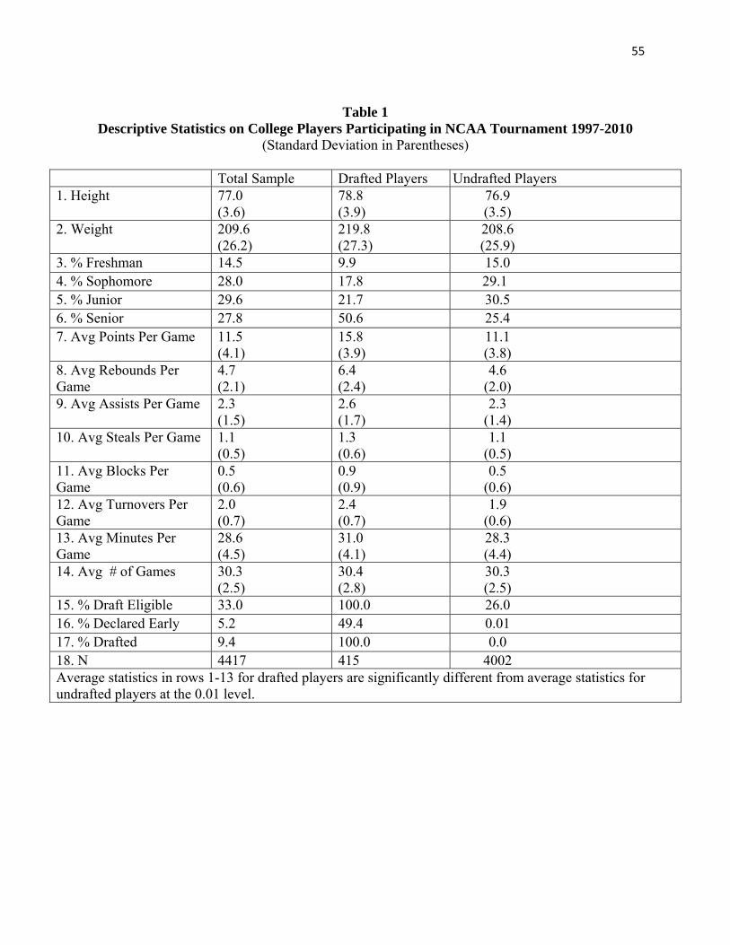
55 

 

Table 1 Descriptive Statistics on College Players Participating in NCAA Tournament 1997-2010

(Standard Deviation in Parentheses)

Total Sample Drafted Players Undrafted Players 1. Height 77.0

(3.6) 78.8 (3.9)

76.9 (3.5)

2. Weight 209.6 (26.2)

219.8 (27.3)

208.6 (25.9)

3. % Freshman 14.5 9.9 15.0 4. % Sophomore 28.0 17.8 29.1 5. % Junior 29.6 21.7 30.5 6. % Senior 27.8 50.6 25.4 7. Avg Points Per Game 11.5

(4.1) 15.8 (3.9)

11.1 (3.8)

8. Avg Rebounds Per Game

4.7 (2.1)

6.4 (2.4)

4.6 (2.0)

9. Avg Assists Per Game 2.3 (1.5)

2.6 (1.7)

2.3 (1.4)

10. Avg Steals Per Game 1.1 (0.5)

1.3 (0.6)

1.1 (0.5)

11. Avg Blocks Per Game

0.5 (0.6)

0.9 (0.9)

0.5 (0.6)

12. Avg Turnovers Per Game

2.0 (0.7)

2.4 (0.7)

1.9 (0.6)

13. Avg Minutes Per Game

28.6 (4.5)

31.0 (4.1)

28.3 (4.4)

14. Avg # of Games 30.3 (2.5)

30.4 (2.8)

30.3 (2.5)

15. % Draft Eligible 33.0 100.0 26.0 16. % Declared Early 5.2 49.4 0.01 17. % Drafted 9.4 100.0 0.0 18. N 4417 415 4002 Average statistics in rows 1-13 for drafted players are significantly different from average statistics for undrafted players at the 0.01 level.

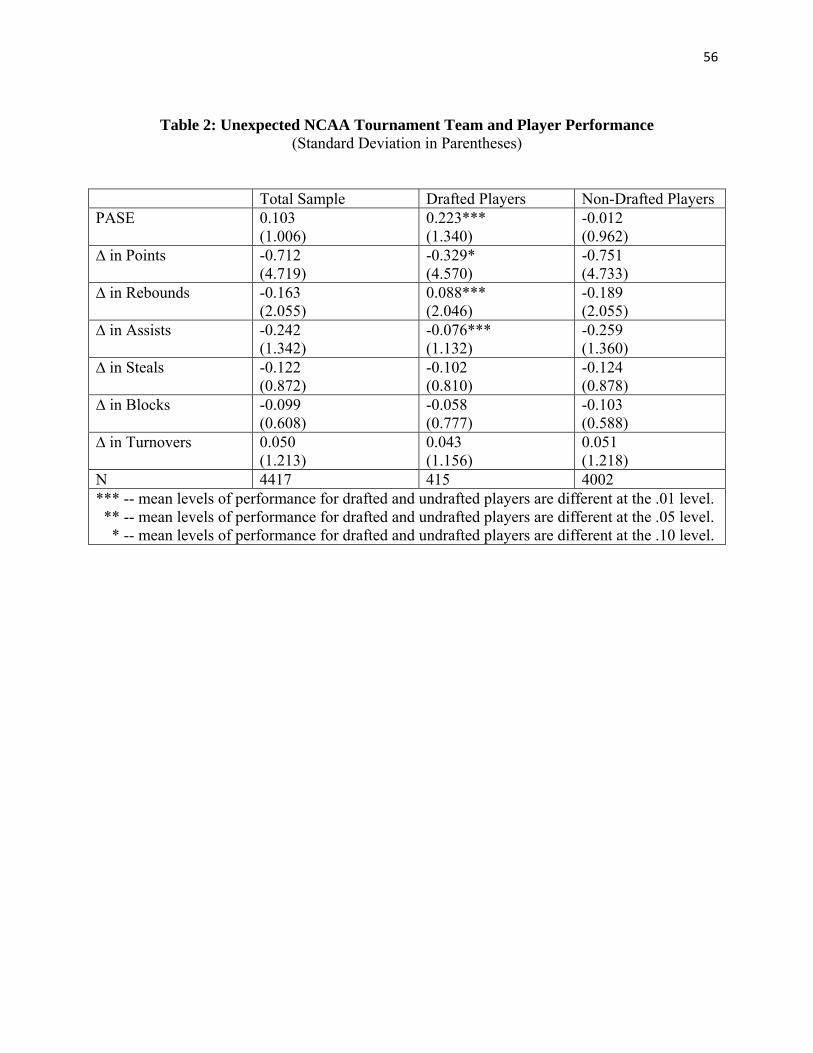
56 

 

Table 2: Unexpected NCAA Tournament Team and Player Performance (Standard Deviation in Parentheses)

Total Sample Drafted Players Non-Drafted Players PASE 0.103

(1.006) 0.223*** (1.340)

-0.012 (0.962)

∆ in Points -0.712 (4.719)

-0.329* (4.570)

-0.751 (4.733)

∆ in Rebounds -0.163 (2.055)

0.088*** (2.046)

-0.189 (2.055)

∆ in Assists -0.242 (1.342)

-0.076*** (1.132)

-0.259 (1.360)

∆ in Steals -0.122 (0.872)

-0.102 (0.810)

-0.124 (0.878)

∆ in Blocks -0.099 (0.608)

-0.058 (0.777)

-0.103 (0.588)

∆ in Turnovers 0.050 (1.213)

0.043 (1.156)

0.051 (1.218)

N 4417 415 4002 *** -- mean levels of performance for drafted and undrafted players are different at the .01 level. ** -- mean levels of performance for drafted and undrafted players are different at the .05 level. * -- mean levels of performance for drafted and undrafted players are different at the .10 level.

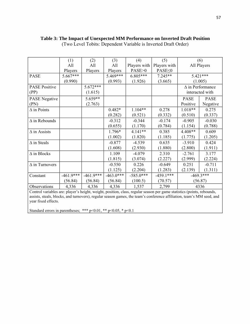
57 

 

Table 3: The Impact of Unexpected MM Performance on Inverted Draft Position (Two Level Tobits: Dependent Variable is Inverted Draft Order)

 

(1) All

Players

(2) All

Players

(3) All

Players

(4) Players with

PASE>0

(5) Players with

PASE≤0

(6) All Players

PASE 5.667*** (0.990)

5.469*** (0.993)

6.805*** (1.926)

7.245** (3.665)

5.421*** (1.005)

PASE Positive (PP)

5.672*** (1.615)

∆ in Performance interacted with

PASE Negative (PN)

5.659** (2.763)

PASE Positive

PASE Negative

∆ in Points 0.482* (0.282)

1.104** (0.521)

0.278 (0.332)

1.018** (0.510)

0.275 (0.337)

∆ in Rebounds -0.312 (0.655)

-0.344 (1.170)

-0.174 (0.784)

-0.905 (1.154)

-0.030 (0.788)

∆ in Assists 1.796* (1.002)

4.141** (1.820)

0.385 (1.185)

4.408** (1.775)

0.609 (1.205)

∆ in Steals -0.877 (1.608)

-4.539 (2.930)

0.635 (1.880)

-3.910 (2.800)

0.424 (1.911)

∆ in Blocks 1.109 (1.815)

-4.079 (3.074)

2.310 (2.227)

-2.761 (2.999)

3.177 (2.224)

∆ in Turnovers -0.550 (1.125)

0.226 (2.204)

-0.649 (1.283)

0.251 (2.139)

-0.711 (1.311)

Constant -461.9*** (56.84)

-461.9***(56.84)

-463.0***(56.84)

-585.0*** (100.5)

-459.1*** (70.57)

-469.3*** (56.87)

Observations 4,336 4,336 4,336 1,537 2,799 4336 Control variables are: player’s height, weight, position, class, regular season per game statistics (points, rebounds, assists, steals, blocks, and turnovers), regular season games, the team’s conference affiliation, team’s MM seed, and year fixed effects. Standard errors in parentheses; *** p<0.01, ** p<0.05, * p<0.1

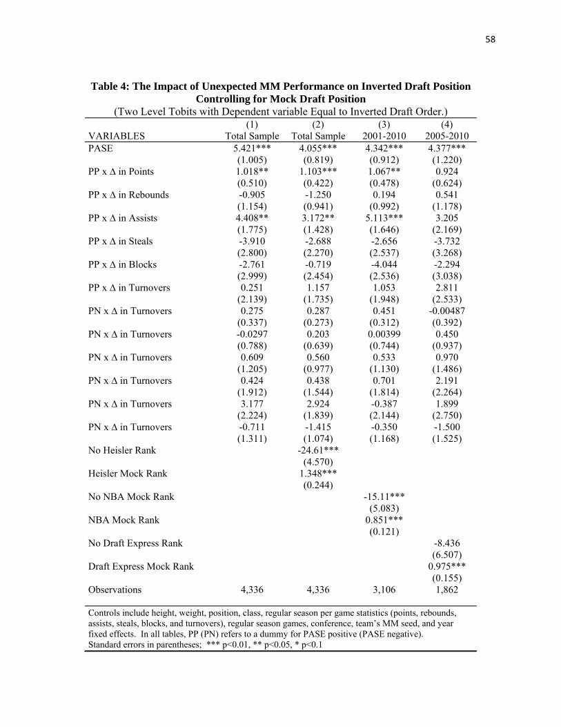
58 

 

Table 4: The Impact of Unexpected MM Performance on Inverted Draft Position Controlling for Mock Draft Position

(Two Level Tobits with Dependent variable Equal to Inverted Draft Order.) (1) (2) (3) (4) VARIABLES Total Sample Total Sample 2001-2010 2005-2010 PASE 5.421*** 4.055*** 4.342*** 4.377*** (1.005) (0.819) (0.912) (1.220) PP x ∆ in Points 1.018** 1.103*** 1.067** 0.924 (0.510) (0.422) (0.478) (0.624) PP x ∆ in Rebounds -0.905 -1.250 0.194 0.541 (1.154) (0.941) (0.992) (1.178) PP x ∆ in Assists 4.408** 3.172** 5.113*** 3.205 (1.775) (1.428) (1.646) (2.169) PP x ∆ in Steals -3.910 -2.688 -2.656 -3.732 (2.800) (2.270) (2.537) (3.268) PP x ∆ in Blocks -2.761 -0.719 -4.044 -2.294 (2.999) (2.454) (2.536) (3.038) PP x ∆ in Turnovers 0.251 1.157 1.053 2.811 (2.139) (1.735) (1.948) (2.533) PN x ∆ in Turnovers 0.275 0.287 0.451 -0.00487 (0.337) (0.273) (0.312) (0.392) PN x ∆ in Turnovers -0.0297 0.203 0.00399 0.450 (0.788) (0.639) (0.744) (0.937) PN x ∆ in Turnovers 0.609 0.560 0.533 0.970 (1.205) (0.977) (1.130) (1.486) PN x ∆ in Turnovers 0.424 0.438 0.701 2.191 (1.912) (1.544) (1.814) (2.264) PN x ∆ in Turnovers 3.177 2.924 -0.387 1.899 (2.224) (1.839) (2.144) (2.750) PN x ∆ in Turnovers -0.711 -1.415 -0.350 -1.500 (1.311) (1.074) (1.168) (1.525) No Heisler Rank -24.61*** (4.570) Heisler Mock Rank 1.348*** (0.244) No NBA Mock Rank -15.11*** (5.083) NBA Mock Rank 0.851*** (0.121) No Draft Express Rank -8.436 (6.507) Draft Express Mock Rank 0.975*** (0.155) Observations 4,336 4,336 3,106 1,862

Controls include height, weight, position, class, regular season per game statistics (points, rebounds, assists, steals, blocks, and turnovers), regular season games, conference, team’s MM seed, and year fixed effects. In all tables, PP (PN) refers to a dummy for PASE positive (PASE negative). Standard errors in parentheses; *** p<0.01, ** p<0.05, * p<0.1

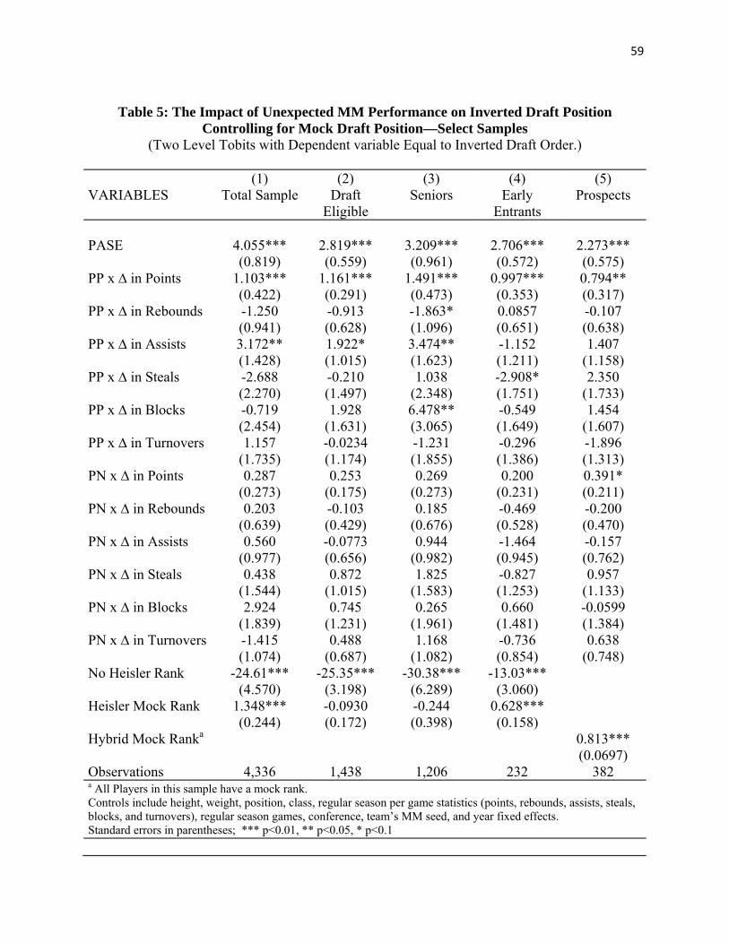
59 

 

Table 5: The Impact of Unexpected MM Performance on Inverted Draft Position Controlling for Mock Draft Position—Select Samples

(Two Level Tobits with Dependent variable Equal to Inverted Draft Order.)

(1) (2) (3) (4) (5) VARIABLES Total Sample Draft

Eligible Seniors Early

Entrants Prospects

PASE 4.055*** 2.819*** 3.209*** 2.706*** 2.273*** (0.819) (0.559) (0.961) (0.572) (0.575) PP x ∆ in Points 1.103*** 1.161*** 1.491*** 0.997*** 0.794** (0.422) (0.291) (0.473) (0.353) (0.317) PP x ∆ in Rebounds -1.250 -0.913 -1.863* 0.0857 -0.107 (0.941) (0.628) (1.096) (0.651) (0.638) PP x ∆ in Assists 3.172** 1.922* 3.474** -1.152 1.407 (1.428) (1.015) (1.623) (1.211) (1.158) PP x ∆ in Steals -2.688 -0.210 1.038 -2.908* 2.350 (2.270) (1.497) (2.348) (1.751) (1.733) PP x ∆ in Blocks -0.719 1.928 6.478** -0.549 1.454 (2.454) (1.631) (3.065) (1.649) (1.607) PP x ∆ in Turnovers 1.157 -0.0234 -1.231 -0.296 -1.896 (1.735) (1.174) (1.855) (1.386) (1.313) PN x ∆ in Points 0.287 0.253 0.269 0.200 0.391* (0.273) (0.175) (0.273) (0.231) (0.211) PN x ∆ in Rebounds 0.203 -0.103 0.185 -0.469 -0.200 (0.639) (0.429) (0.676) (0.528) (0.470) PN x ∆ in Assists 0.560 -0.0773 0.944 -1.464 -0.157 (0.977) (0.656) (0.982) (0.945) (0.762) PN x ∆ in Steals 0.438 0.872 1.825 -0.827 0.957 (1.544) (1.015) (1.583) (1.253) (1.133) PN x ∆ in Blocks 2.924 0.745 0.265 0.660 -0.0599 (1.839) (1.231) (1.961) (1.481) (1.384) PN x ∆ in Turnovers -1.415 0.488 1.168 -0.736 0.638 (1.074) (0.687) (1.082) (0.854) (0.748) No Heisler Rank -24.61*** -25.35*** -30.38*** -13.03*** (4.570) (3.198) (6.289) (3.060) Heisler Mock Rank 1.348*** -0.0930 -0.244 0.628*** (0.244) (0.172) (0.398) (0.158) Hybrid Mock Ranka 0.813*** (0.0697) Observations 4,336 1,438 1,206 232 382 a All Players in this sample have a mock rank. Controls include height, weight, position, class, regular season per game statistics (points, rebounds, assists, steals, blocks, and turnovers), regular season games, conference, team’s MM seed, and year fixed effects. Standard errors in parentheses; *** p<0.01, ** p<0.05, * p<0.1

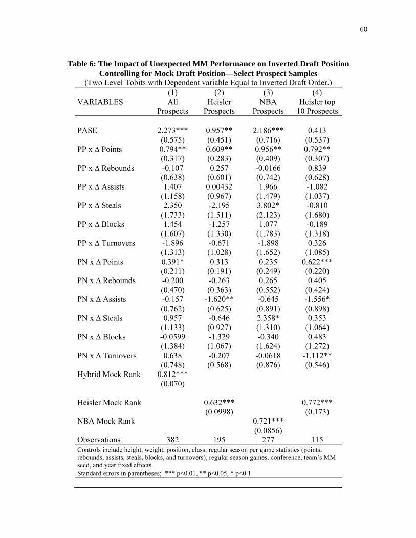
60 

 

Table 6: The Impact of Unexpected MM Performance on Inverted Draft Position Controlling for Mock Draft Position—Select Prospect Samples

(Two Level Tobits with Dependent variable Equal to Inverted Draft Order.) (1) (2) (3) (4)

VARIABLES All Prospects

Heisler Prospects

NBA Prospects

Heisler top 10 Prospects

PASE 2.273*** 0.957** 2.186*** 0.413 (0.575) (0.451) (0.716) (0.537) PP x ∆ Points 0.794** 0.609** 0.956** 0.792** (0.317) (0.283) (0.409) (0.307) PP x ∆ Rebounds -0.107 0.257 -0.0166 0.839 (0.638) (0.601) (0.742) (0.628) PP x ∆ Assists 1.407 0.00432 1.966 -1.082 (1.158) (0.967) (1.479) (1.037) PP x ∆ Steals 2.350 -2.195 3.802* -0.810 (1.733) (1.511) (2.123) (1.680) PP x ∆ Blocks 1.454 -1.257 1.077 -0.189 (1.607) (1.330) (1.783) (1.318) PP x ∆ Turnovers -1.896 -0.671 -1.898 0.326 (1.313) (1.028) (1.652) (1.085) PN x ∆ Points 0.391* 0.313 0.235 0.622*** (0.211) (0.191) (0.249) (0.220) PN x ∆ Rebounds -0.200 -0.263 0.265 0.405 (0.470) (0.363) (0.552) (0.424) PN x ∆ Assists -0.157 -1.620** -0.645 -1.556* (0.762) (0.625) (0.891) (0.898) PN x ∆ Steals 0.957 -0.646 2.358* 0.353 (1.133) (0.927) (1.310) (1.064) PN x ∆ Blocks -0.0599 -1.329 -0.340 0.483 (1.384) (1.067) (1.624) (1.272) PN x ∆ Turnovers 0.638 -0.207 -0.0618 -1.112** (0.748) (0.568) (0.876) (0.546) Hybrid Mock Rank 0.812***

(0.070)

Heisler Mock Rank 0.632*** 0.772*** (0.0998) (0.173) NBA Mock Rank 0.721*** (0.0856) Observations 382 195 277 115 Controls include height, weight, position, class, regular season per game statistics (points, rebounds, assists, steals, blocks, and turnovers), regular season games, conference, team’s MM seed, and year fixed effects. Standard errors in parentheses; *** p<0.01, ** p<0.05, * p<0.1

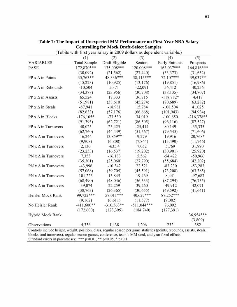
61 

 

 

Table 7: The Impact of Unexpected MM Performance on First Year NBA Salary Controlling for Mock Draft-Select Samples

(Tobits with first year salary in 2009 dollars as dependent variable.) (1) (2) (3) (4) (5) VARIABLES Total Sample Draft Eligible Seniors Early Entrants Prospects PASE 172,870*** 135,008*** 120,008*** 163,037*** 164,816*** (30,092) (21,562) (27,440) (33,373) (31,652) PP x ∆ in Points 35,763** 48,336*** 38,115*** 72,107*** 39,037** (15,223) (10,925) (13,176) (19,851) (16,986) PP x ∆ in Rebounds -10,504 5,371 -22,091 56,412 40,256 (34,388) (23,956) (30,708) (38,135) (34,807) PP x ∆ in Assists 65,524 17,333 36,715 -118,782* 4,417 (51,981) (38,610) (45,274) (70,689) (63,282) PP x ∆ in Steals -87,941 -18,981 15,784 -108,504 41,025 (82,633) (57,176) (66,668) (101,943) (94,934) PP x ∆ in Blocks -176,105* -73,530 34,019 -100,650 -216,378** (91,393) (62,721) (86,505) (96,116) (87,527) PP x ∆ in Turnovers 40,025 25,425 -25,414 80,149 -35,335 (62,760) (44,449) (51,567) (79,545) (71,606) PN x ∆ in Turnovers 16,244 13,859** 9,279 19,916 20,768* (9,908) (6,808) (7,844) (13,490) (11,746) PN x ∆ in Turnovers 2,130 -635.4 7,052 5,769 31,990 (23,253) (16,537) (19,202) (30,901) (25,920) PN x ∆ in Turnovers 7,353 -16,183 5,562 -54,422 -50,966 (35,301) (25,060) (27,790) (55,684) (42,202) PN x ∆ in Turnovers -43,996 -10,342 22,521 -83,230 -53,283 (57,068) (39,705) (45,591) (73,208) (63,385) PN x ∆ in Turnovers 101,223 13,845 19,469 8,441 -97,687 (68,490) (48,046) (56,333) (87,294) (76,735) PN x ∆ in Turnovers -39,074 22,259 39,260 -49,912 42,071 (38,763) (26,365) (30,655) (49,592) (41,641) Heisler Mock Rank 99,722*** 57,011*** 40,627*** 87,252*** (9,162) (6,611) (11,577) (9,082) No Heisler Rank -411,600** -310,563** -511,044*** 76,092 (172,600) (123,395) (184,740) (177,391) Hybrid Mock Rank 36,954*** (3,809) Observations 4,336 1,438 1,206 232 382 Controls include height, weight, position, class, regular season per game statistics (points, rebounds, assists, steals, blocks, and turnovers), regular season games, conference, team’s MM seed, and year fixed effects. Standard errors in parentheses; *** p<0.01, ** p<0.05, * p<0.1

 

 

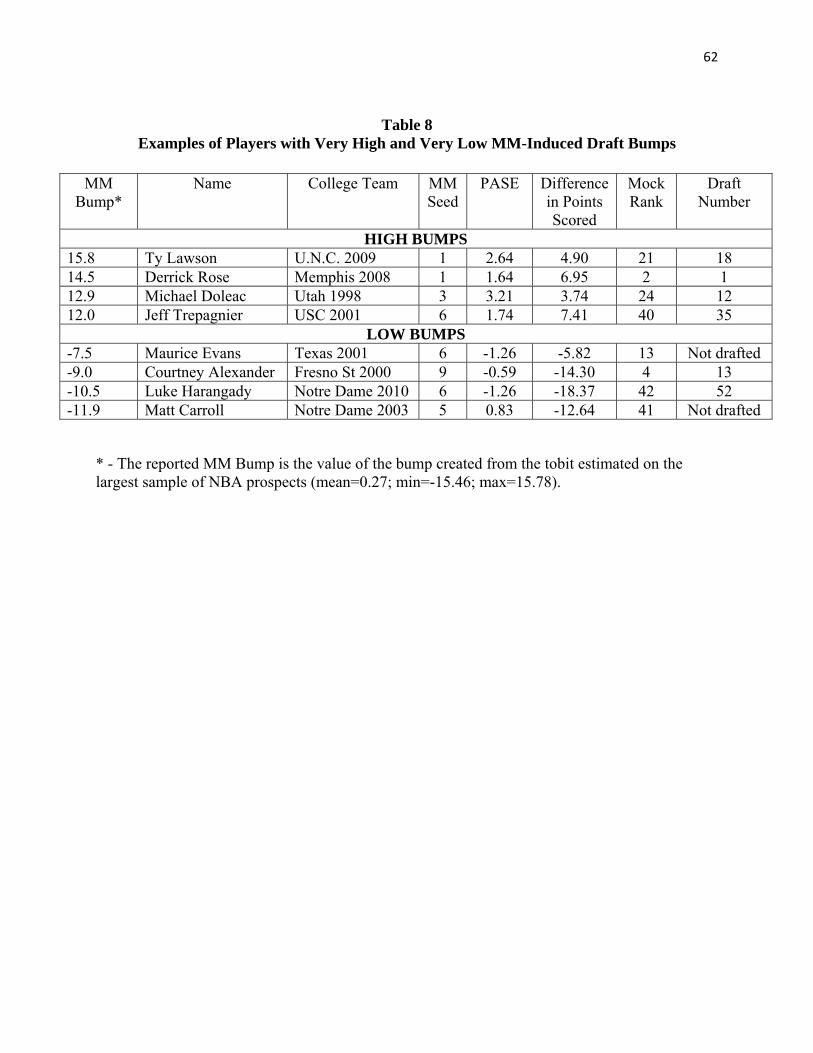
62 

 

Table 8 Examples of Players with Very High and Very Low MM-Induced Draft Bumps

MM

Bump* Name College Team MM

Seed PASE Difference

in Points Scored

Mock Rank

Draft Number

HIGH BUMPS 15.8 Ty Lawson U.N.C. 2009 1 2.64 4.90 21 18 14.5 Derrick Rose Memphis 2008 1 1.64 6.95 2 1 12.9 Michael Doleac Utah 1998 3 3.21 3.74 24 12 12.0 Jeff Trepagnier USC 2001 6 1.74 7.41 40 35

LOW BUMPS -7.5 Maurice Evans Texas 2001 6 -1.26 -5.82 13 Not drafted -9.0 Courtney Alexander Fresno St 2000 9 -0.59 -14.30 4 13 -10.5 Luke Harangady Notre Dame 2010 6 -1.26 -18.37 42 52 -11.9 Matt Carroll Notre Dame 2003 5 0.83 -12.64 41 Not drafted

* - The reported MM Bump is the value of the bump created from the tobit estimated on the largest sample of NBA prospects (mean=0.27; min=-15.46; max=15.78).  

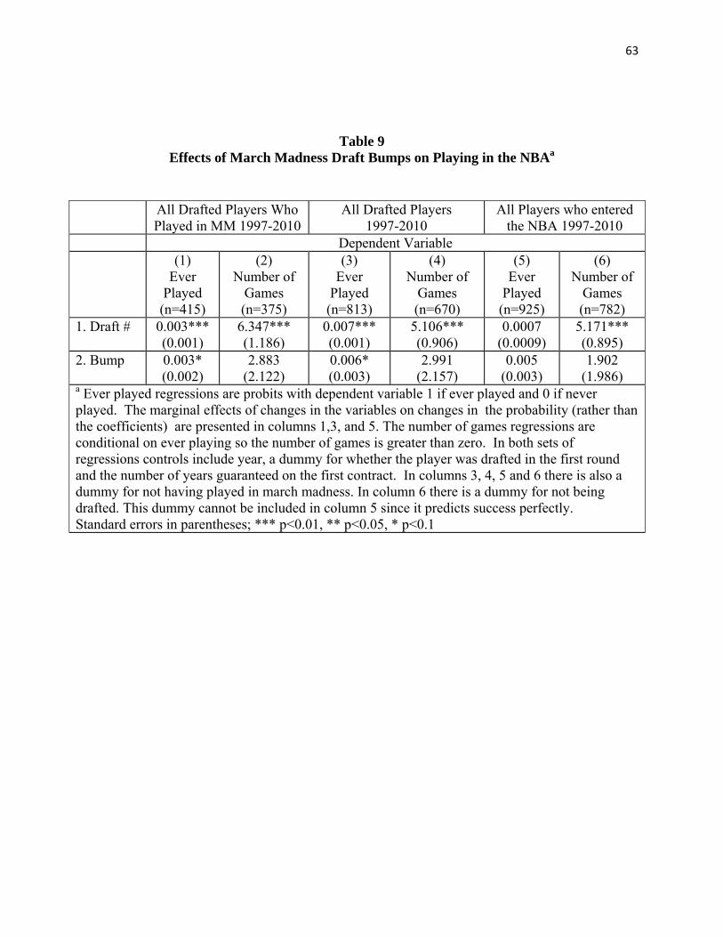
63 

 

 

Table 9 Effects of March Madness Draft Bumps on Playing in the NBAa

All Drafted Players Who Played in MM 1997-2010

All Drafted Players 1997-2010

All Players who entered the NBA 1997-2010

Dependent Variable (1)

Ever Played

(n=415)

(2) Number of

Games (n=375)

(3) Ever

Played (n=813)

(4) Number of

Games (n=670)

(5) Ever

Played (n=925)

(6) Number of

Games (n=782)

1. Draft # 0.003*** (0.001)

6.347*** (1.186)

0.007*** (0.001)

5.106*** (0.906)

0.0007 (0.0009)

5.171*** (0.895)

2. Bump 0.003* (0.002)

2.883 (2.122)

0.006* (0.003)

2.991 (2.157)

0.005 (0.003)

1.902 (1.986)

a Ever played regressions are probits with dependent variable 1 if ever played and 0 if never played. The marginal effects of changes in the variables on changes in the probability (rather than the coefficients) are presented in columns 1,3, and 5. The number of games regressions are conditional on ever playing so the number of games is greater than zero. In both sets of regressions controls include year, a dummy for whether the player was drafted in the first round and the number of years guaranteed on the first contract. In columns 3, 4, 5 and 6 there is also a dummy for not having played in march madness. In column 6 there is a dummy for not being drafted. This dummy cannot be included in column 5 since it predicts success perfectly. Standard errors in parentheses; *** p<0.01, ** p<0.05, * p<0.1

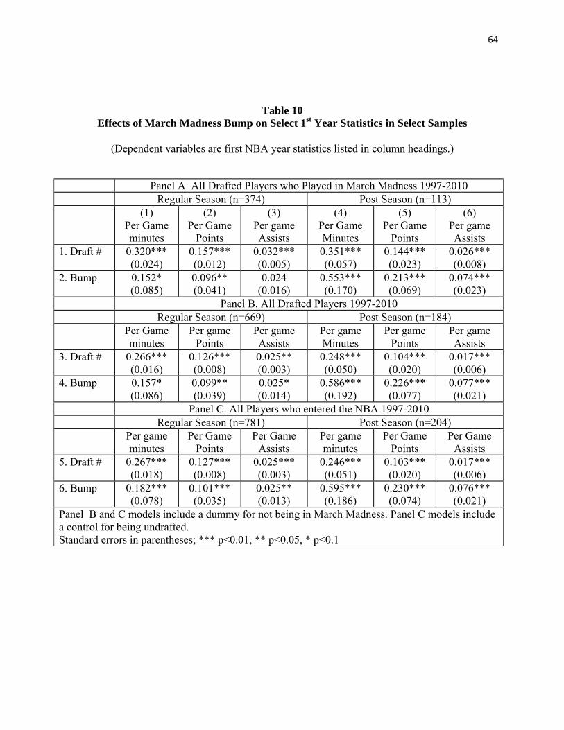
64 

 

Table 10 Effects of March Madness Bump on Select 1st Year Statistics in Select Samples

(Dependent variables are first NBA year statistics listed in column headings.)

Panel A. All Drafted Players who Played in March Madness 1997-2010 Regular Season (n=374) Post Season (n=113)

(1) Per Game minutes

(2) Per Game

Points

(3) Per game Assists

(4) Per Game Minutes

(5) Per Game

Points

(6) Per game Assists

1. Draft # 0.320*** (0.024)

0.157*** (0.012)

0.032*** (0.005)

0.351*** (0.057)

0.144*** (0.023)

0.026*** (0.008)

2. Bump 0.152* (0.085)

0.096** (0.041)

0.024 (0.016)

0.553*** (0.170)

0.213*** (0.069)

0.074*** (0.023)

Panel B. All Drafted Players 1997-2010 Regular Season (n=669) Post Season (n=184)

Per Game minutes

Per game Points

Per game Assists

Per game Minutes

Per game Points

Per game Assists

3. Draft # 0.266*** (0.016)

0.126*** (0.008)

0.025** (0.003)

0.248*** (0.050)

0.104*** (0.020)

0.017*** (0.006)

4. Bump 0.157* (0.086)

0.099** (0.039)

0.025* (0.014)

0.586*** (0.192)

0.226*** (0.077)

0.077*** (0.021)

Panel C. All Players who entered the NBA 1997-2010 Regular Season (n=781) Post Season (n=204)

Per game minutes

Per Game Points

Per Game Assists

Per game minutes

Per Game Points

Per Game Assists

5. Draft # 0.267*** (0.018)

0.127*** (0.008)

0.025*** (0.003)

0.246*** (0.051)

0.103*** (0.020)

0.017*** (0.006)

6. Bump 0.182*** (0.078)

0.101*** (0.035)

0.025** (0.013)

0.595*** (0.186)

0.230*** (0.074)

0.076*** (0.021)

Panel B and C models include a dummy for not being in March Madness. Panel C models include a control for being undrafted. Standard errors in parentheses; *** p<0.01, ** p<0.05, * p<0.1

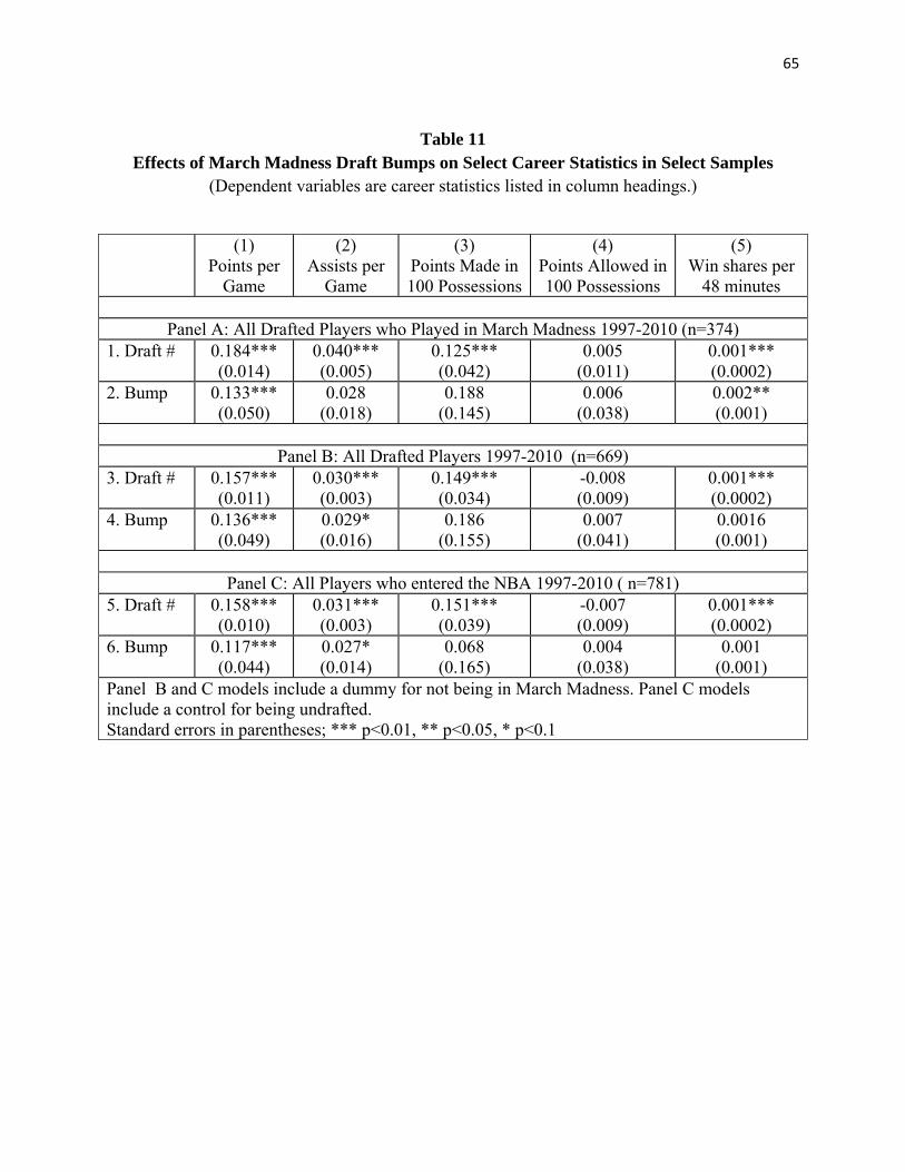
65 

 

Table 11 Effects of March Madness Draft Bumps on Select Career Statistics in Select Samples

(Dependent variables are career statistics listed in column headings.)

(1) Points per

Game

(2) Assists per

Game

(3) Points Made in 100 Possessions

(4) Points Allowed in 100 Possessions

(5) Win shares per

48 minutes

Panel A: All Drafted Players who Played in March Madness 1997-2010 (n=374) 1. Draft # 0.184***

(0.014) 0.040*** (0.005)

0.125*** (0.042)

0.005 (0.011)

0.001*** (0.0002)

2. Bump 0.133*** (0.050)

0.028 (0.018)

0.188 (0.145)

0.006 (0.038)

0.002** (0.001)

Panel B: All Drafted Players 1997-2010 (n=669)

3. Draft # 0.157*** (0.011)

0.030*** (0.003)

0.149*** (0.034)

-0.008 (0.009)

0.001*** (0.0002)

4. Bump 0.136*** (0.049)

0.029* (0.016)

0.186 (0.155)

0.007 (0.041)

0.0016 (0.001)

Panel C: All Players who entered the NBA 1997-2010 ( n=781)

5. Draft # 0.158*** (0.010)

0.031*** (0.003)

0.151*** (0.039)

-0.007 (0.009)

0.001*** (0.0002)

6. Bump 0.117*** (0.044)

0.027* (0.014)

0.068 (0.165)

0.004 (0.038)

0.001 (0.001)

Panel B and C models include a dummy for not being in March Madness. Panel C models include a control for being undrafted. Standard errors in parentheses; *** p<0.01, ** p<0.05, * p<0.1

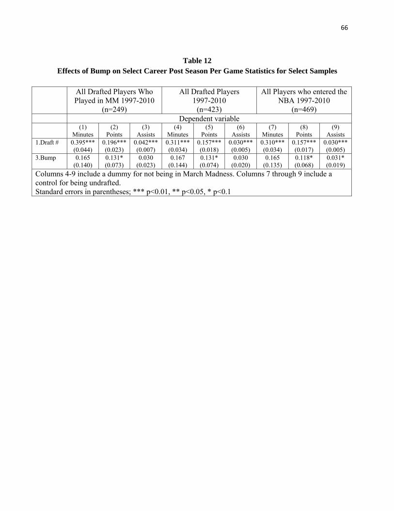
66 

 

Table 12 Effects of Bump on Select Career Post Season Per Game Statistics for Select Samples

All Drafted Players Who

Played in MM 1997-2010 (n=249)

All Drafted Players 1997-2010

(n=423)

All Players who entered the NBA 1997-2010

(n=469) Dependent variable

(1) Minutes

(2) Points

(3) Assists

(4) Minutes

(5) Points

(6) Assists

(7) Minutes

(8) Points

(9) Assists

1.Draft # 0.395*** (0.044)

0.196*** (0.023)

0.042*** (0.007)

0.311*** (0.034)

0.157*** (0.018)

0.030*** (0.005)

0.310*** (0.034)

0.157*** (0.017)

0.030*** (0.005)

3.Bump 0.165 (0.140)

0.131* (0.073)

0.030 (0.023)

0.167 (0.144)

0.131* (0.074)

0.030 (0.020)

0.165 (0.135)

0.118* (0.068)

0.031* (0.019)

Columns 4-9 include a dummy for not being in March Madness. Columns 7 through 9 include a control for being undrafted. Standard errors in parentheses; *** p<0.01, ** p<0.05, * p<0.1

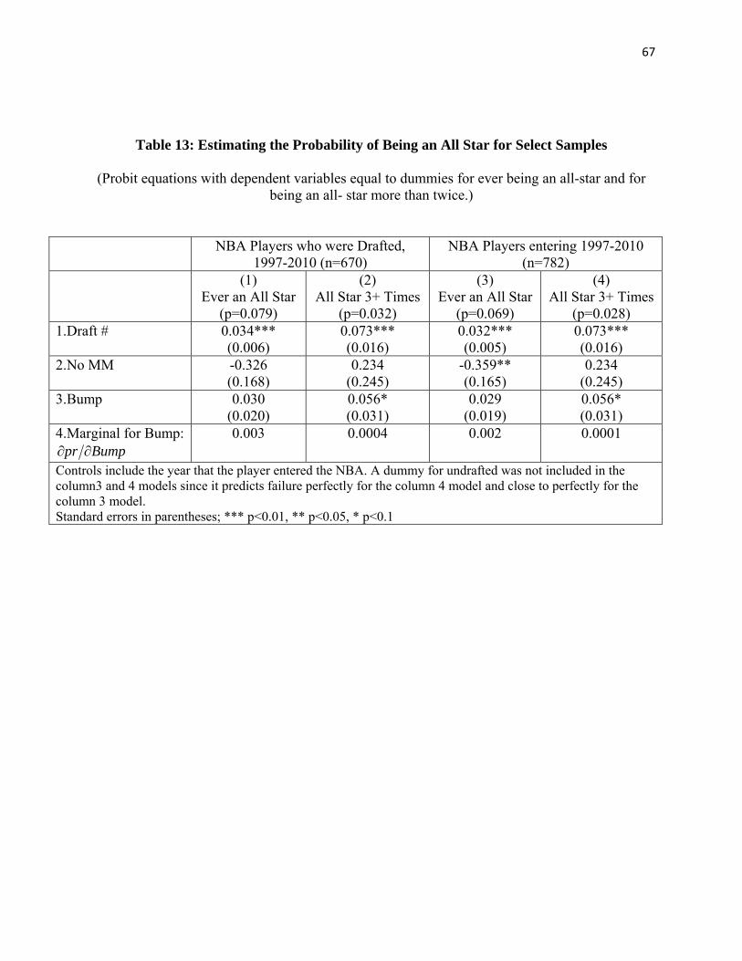
67 

 

 

Table 13: Estimating the Probability of Being an All Star for Select Samples

(Probit equations with dependent variables equal to dummies for ever being an all-star and for being an all- star more than twice.)

NBA Players who were Drafted, 1997-2010 (n=670)

NBA Players entering 1997-2010 (n=782)

(1) Ever an All Star

(p=0.079)

(2) All Star 3+ Times

(p=0.032)

(3) Ever an All Star

(p=0.069)

(4) All Star 3+ Times

(p=0.028) 1.Draft # 0.034***

(0.006) 0.073*** (0.016)

0.032*** (0.005)

0.073*** (0.016)

2.No MM -0.326 (0.168)

0.234 (0.245)

-0.359** (0.165)

0.234 (0.245)

3.Bump 0.030 (0.020)

0.056* (0.031)

0.029 (0.019)

0.056* (0.031)

4.Marginal for Bump: Bumppr

0.003 0.0004 0.002 0.0001

Controls include the year that the player entered the NBA. A dummy for undrafted was not included in the column3 and 4 models since it predicts failure perfectly for the column 4 model and close to perfectly for the column 3 model. Standard errors in parentheses; *** p<0.01, ** p<0.05, * p<0.1

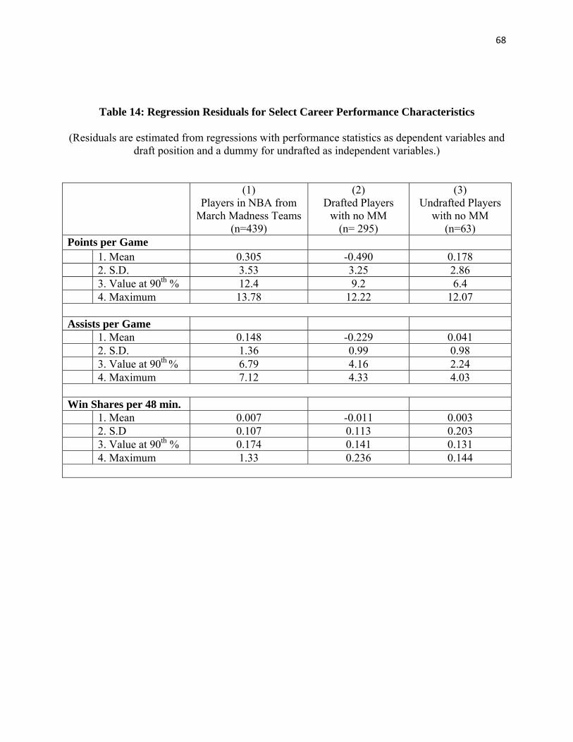
68 

 

 

Table 14: Regression Residuals for Select Career Performance Characteristics

(Residuals are estimated from regressions with performance statistics as dependent variables and draft position and a dummy for undrafted as independent variables.)

(1) Players in NBA from

March Madness Teams (n=439)

(2) Drafted Players

with no MM (n= 295)

(3) Undrafted Players

with no MM (n=63)

Points per Game 1. Mean 0.305 -0.490 0.178 2. S.D. 3.53 3.25 2.86 3. Value at 90th % 12.4 9.2 6.4 4. Maximum 13.78 12.22 12.07 Assists per Game 1. Mean 0.148 -0.229 0.041 2. S.D. 1.36 0.99 0.98 3. Value at 90th % 6.79 4.16 2.24 4. Maximum 7.12 4.33 4.03 Win Shares per 48 min. 1. Mean 0.007 -0.011 0.003 2. S.D 0.107 0.113 0.203 3. Value at 90th % 0.174 0.141 0.131 4. Maximum 1.33 0.236 0.144

69 

 

Appendix Table

Data Sources on NCAA Basketball Tournament, Collegiate Players and NBA Players

StatSheet o http://statsheet.com/ o College player/team game statistics

LA Times

o http://articles.latimes.com/2010/mar/21/sports/la-sp-heisler-20100321 o 1996-2010 Heisler Mock Drafts

DraftExpress

o http://www.draftexpress.com o List of prospects 2006-2008, additional mock draft data for limited years

NBA.com

o http://www.nba.com o List of prospects 2001-2010, additional mock draft data for limited years

DatabaseSports.com

o http://www.databasesports.com/ncaab/index.htm o NCAA March Madness Results, and NBA Drafts

Basketball-Reference

o http://www.basketball-reference.com/ o NBA player game statistics, salaries, and career stastistics