Embed Size (px)
Citation preview
Brigham Young University Brigham Young University
BYU ScholarsArchive BYU ScholarsArchive
Theses and Dissertations
2017-07-01
Does Marijuana Decriminalization Make the Roads More Does Marijuana Decriminalization Make the Roads More
Dangerous? Dangerous?
Daehyeon Kim Brigham Young University
Follow this and additional works at: https://scholarsarchive.byu.edu/etd
Part of the Sociology Commons
BYU ScholarsArchive Citation BYU ScholarsArchive Citation Kim, Daehyeon, "Does Marijuana Decriminalization Make the Roads More Dangerous?" (2017). Theses and Dissertations. 6490. https://scholarsarchive.byu.edu/etd/6490
This Thesis is brought to you for free and open access by BYU ScholarsArchive. It has been accepted for inclusion in Theses and Dissertations by an authorized administrator of BYU ScholarsArchive. For more information, please contact [email protected], [email protected].
Does Marijuana Decriminalization Make the Roads More Dangerous?
Daehyeon Kim
A thesis submitted to the faculty of Brigham Young University
in partial fulfillment of the requirements for the degree of
Master of Science
John P. Hoffmann, Chair Eric C. Dahlin
Lance D. Erickson
Department of Sociology
Brigham Young University
Copyright © 2017 Daehyeon Kim
All Rights Reserved

ABSTRACT
Does Marijuana Decriminalization Make the Roads More Dangerous?
Daehyeon Kim Department of Sociology, BYU
Master of Science
As the movement to decriminalize marijuana has gained more support throughout the United States, as of early 2017, 21 states have decriminalized the possession of a small amount of marijuana for personal recreational use, and more states are expected to decriminalize marijuana (GOVERNING 2017). Despite this strong move toward decriminalizing marijuana, however, the consequences of implementing such a policy are still very much unknown. One of the concerns regarding this movement to decriminalize marijuana is its potential impact on road safety (Schrader 2015; Roberts 2017; Halsey 2016). Although there are a few studies that have examined the association between marijuana use and availability and traffic fatalities, these studies are correlational in nature and show divergent outcomes (Anderson et al. 2011; Anderson and Ree 2014). Furthermore, these studies do not examine the impact of decriminalizing marijuana on road safety. In order to fill this gap, my research investigates the causal association between marijuana decriminalization and traffic fatalities by using the synthetic control method, pioneered by Abadie et al. (2010). This study estimates the causal effects of 2009 Massachusetts’s marijuana decriminalization on Massachusetts’ total traffic fatalities by comparing Massachusetts’s trends in total traffic fatalities and its synthetic counterpart. The results of this study show a temporary increase in the number of total traffic fatalities in Massachusetts compared to its synthetic counterpart between 2009 and 2012, suggesting marijuana decriminalization’s detrimental effect on road safety. Future studies should consider investigating the heterogeneous effects of marijuana decriminalization on traffic fatalities based on age groups, gender, and residential density and the causal mechanism between marijuana decriminalization and traffic fatalities.
Keywords: marijuana, marijuana decriminalization, traffic fatalities, road safety, policy

ACKNOWLEDGEMENTS
Without the tremendous help and support from Professor Hoffmann, I would have not
even dreamed of writing a thesis using the synthetic control method. Thank you so much for
always challenging me to learn more and to dream big and believing in me. Furthermore, without
the help of my committee and many others, I would have not been able to improve and complete
my thesis. I express my gratitude to Professor Dahlin, Professor Erickson, Professor Dufur, and
Ms. McCabe, who is the department secretary of the sociology department.
Without the encouragement and support from Professor Forste, I would have not joined
the sociology master’s program at Brigham Young University two years ago. If I had not met
you, I am not sure where I would be now. Thank you so much for everything that you have done
for me.
Margaret, thank you so much for always reminding me of all the deadlines and making
sure that I am on top of everything. Without your help, I am sure that I would have missed many
deadlines.
The past two years has been a great learning experience for me both professionally and
personally. Thank you every professor who has inspired me to become an academic who has a
desire to serve others who walk into my life. To my friends in the sociology graduate program,
thank you for your encouragement, support, and friendship. I am so grateful that I have become
friends and colleagues with you all. You guys are great.
Thank you everyone who has helped me continue my education. I owe a lot to you all. I
will try my best to become an individual who helps others to reach their full potential as you
have helped me.
iv
TABLE OF CONTENTS ABSTRACT .................................................................................................................................... ii ACKNOWLEDGEMENTS ........................................................................................................... iii LIST OF TABLES .......................................................................................................................... v
LIST OF FIGURES ....................................................................................................................... vi INTRODUCTION .......................................................................................................................... 1 LITERATURE REVIEW ............................................................................................................... 2
The History of Marijuana Decriminalization in the United States ............................................. 2
The 2009 Massachusetts Marijuana Decriminalization Initiative .............................................. 3 Marijuana Decriminalization and Marijuana Consumption ....................................................... 5
Marijuana Use and Availability and Traffic Fatalities ............................................................... 6
HYPOTHESES ............................................................................................................................... 8 DATA & METHODS ..................................................................................................................... 8
Sample and Data ......................................................................................................................... 8
Treatment Condition and Outcome Variable .............................................................................. 9 Predictors of the Outcome of Interest ......................................................................................... 9
Identifying Strategy and Analyses ............................................................................................ 13
RESULTS ..................................................................................................................................... 18 Constructing Synthetic Control and Analysis ........................................................................... 18
Placebo Tests ............................................................................................................................ 21 DISCUSSION ............................................................................................................................... 25
REFERENCES ............................................................................................................................. 28
TABLES ....................................................................................................................................... 32 FIGURES ...................................................................................................................................... 34
APPENDIX ................................................................................................................................... 39

v
LIST OF TABLES
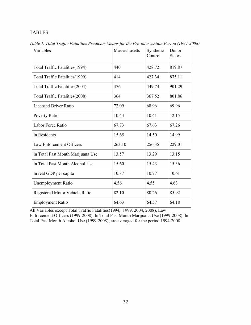
Table 1. Total Traffic Fatalities Predictor Means for the Pre-intervention Period (1994-2008) .. 32
Table 2. Synthetic Control Weights .............................................................................................. 33
vi
LIST OF FIGURES Figure 1. Trends in Total Traffic Fatalities in Massachusetts, the Donor States Average, and the USA Average ................................................................................................................................ 34 Figure 2. Trends in Total Traffic Fatalities in Massachusetts ...................................................... 35 Figure 3. The Gap in Total Traffic Fatalities in All Donor States and Massachusetts ................. 36 Figure 4. The Gap in Total Traffic Fatalities in Selected Donor States and Massachusetts......... 37 Figure 5. Ratio of Post-Marijuana Decriminalization RMSPE to Pre-Marijuana Decriminalization: Massachusetts and Control States .................................................................. 38
1
Does Marijuana Decriminalization Make the Roads More Dangerous?
According to a recent survey by Pew Research Center (2016), the average American’s
attitude towards marijuana use has become more tolerant over the past three decades. Compared
to 1990, when only about 16% of Americans ages 18 or older supported marijuana legalization,
in 2015 this had increased to about 53% (Pew Research Center 2016). As views toward
marijuana use have softened, the movement to decriminalize marijuana has also gained more
support throughout the United States, and, as of early 2017, 21 states have decriminalized the
possession of a small amount of marijuana for personal recreational use. In addition, eight states
have legalized recreational marijuana and 28 states have legalized medical marijuana
(GOVERNING 2017).
Although support for relaxing marijuana laws has been increasing in recent years, the
potential ramifications of decreasing or eliminating penalties for possession and use of marijuana
through medical marijuana availability, decriminalization, or legalization are not clear. For
example, as the laws about marijuana use among adults are relaxed or eliminated, will marijuana
use among youth increase? Will there be more problems with marijuana dependence and abuse?
Will crimes associated with intoxication–such as public nuisance offenses–increase?
Additionally, whereas driving offenses associated with alcohol, such as driving under the
influence (DUI) and driving while intoxicated (DWI), are a concern of many, there is also the
related issue of driving under the influence of marijuana, which, in turn, is likely to make the
roads more dangerous, leading to an increase in traffic fatalities (Schrader 2015; Roberts 2017;
Halsey 2016). Thus, one of the potential ramifications that should be investigated is whether
relaxing marijuana laws has an influence on the number of traffic fatalities. This will help us
understand whether relaxing marijuana laws makes the roads more hazardous.
2
Recently, several media stories about DUI cases in which drivers were detected to be
under the influence of marijuana have raised the public’s concern about the effect of relaxing
marijuana laws on road safety (Schrader 2015; Roberts 2017; Halsey 2016). The research
literature to date generally does not support the argument that changing marijuana laws affects
traffic fatalities, however (Anderson et al. 2011; Anderson and Ree 2014). Nevertheless, this
research has been correlational in nature. As a result, the association between medical marijuana
availiability and road saftey found from this research is likely spurious. Furthermore, this
research has focused on the availability of medical marijuana rather than marijuana
decriminalization. Thus, it is important to consider whether marijuana decriminalization has any
effect on traffic fatalities. To date, no study has considered this issue.
In this study, I examine the impact of the 2009 Massachusetts marijuana
decriminalization legislation on traffic fatalities to investigate the causal effect of marijuana
decriminalization on traffic fatalities. Using a synthetic control method (SCM) (Abadie et al.
2010), I compare the trend in traffic fatalities in Massachusetts (the treated unit) to the traffic
fatalities in a synthetic control – based on characteristics of similar states that did not
decriminalize marijuana – to determine if there are differences in these trends. If there are
differences in trends in traffic fatalities in Massachusetts relative to those in the synthetic control,
this suggests that marijuana decriminalization caused a shift in this outcome of interest.
LITERATURE REVIEW
The History of Marijuana Decriminalization in the United States
The history of marijuana decriminalization in the United States traces back to the 1960s.
In this decade, recreational marijuana use increased throughout the United States. Consequently,
the public’s view of marijuana use became more tolerant. Although marijuana possession
3
remained illegal at the federal level, this more tolerant view led several states to experiment with
marijuana decriminalization in the 1970s. For example, in 1973 Oregon became the first state to
decriminalize marijuana possession (Hardaway 2003). By the end of the 1970s, eight other
states—Alaska, California, Colorado, Mississippi, New York, Nebraska, North Carolina, and
Ohio—passed similar legislation (Davis 2015).
However, by the early 1980s, this movement stalled, partly because several scientific
studies showed that there were various health risks associated with marijuana use. This period
also hailed a rise in the conservative movement in the U.S., with a concomitant emphasis on
deprecating marijuana use. Thus, generally there was little political desire to change marijuana
laws at the state or federal level. In fact, some states, such as Alaska, recriminalized marijuana
use in the 1990s (Davis 2015).
It was not until 2001 that Nevada broke this trend by decriminalizing marijuana (Davis
2015). Since 2001, more states have joined this movement. As of early 2017, 21 states have
decriminalized possession of a small amount of marijuana, and 28 states allow some forms of
medical marijuana based on a physician’s “legal recommendation” since they cannot legally
“prescribe” marijuana under federal law (GOVERNING 2017). Furthermore, eight states and the
District of Columbia have legalized recreational marijuana use for individuals who are 21 years
or older (GOVERNING 2017).
The 2009 Massachusetts Marijuana Decriminalization Initiative
On January 2, 2009, Massachusetts implemented the Massachusetts Sensible Marijuana
Policy initiative, also known as the 2009 Massachusetts marijuana decriminalization law. This
new law reduced the legal penalty for possessing equal to or less than one ounce of marijuana to
a civil infraction with a $100 fine. Previous to this, possession of this amount was deemed a
4
misdemeanor, which could put offenders in jail for up to 6 months with a $500 fine, including a
citation in the CORI criminal records database. However, the new law requires minors to have
their parents informed if they are found in possession of marijuana, with a penalty of community
service and enrollment in drug awareness counseling. If they do not fulfill these requirements,
the law requires them to pay up to a $1,000 fine.
To my knowledge, there have been no studies evaluating the impact of the 2009
Massachusetts marijuana decriminalization law on various social outcomes, such as marijuana
use or road safety. This signifies the need for studies examining the ramifications of this policy.
Massachusetts also legalized medical marijuana on January 1, 2013, and legalized recreational
marijuana on December 15, 2016 (Salsberg 2016). However, given that Massachusetts’s first
medical marijuana dispensary opened on June 24, 2015 and that the data utilized herein are from
1994 to 2014, it is unlikely that these shifts in marijuana policies influence my research
(Marijuana Policy Project 2017). Moreover, the infrastructure for distributing and selling legal
marijuana in Massachusetts is not yet in place.
Massachusetts is an ideal state to study the impact of marijuana decriminalization on
trends in total traffic fatalities. The data used herein range from 1994 to 2014. In order to create a
sound synthetic control, it is generally expected that the data include a sufficient number of
observations during the pre-intervention periods. Furthermore, in order to examine the effect of
the intervention, there should also be a sufficient number of observations during the post-
intervention period. Since Massachusetts implemented its decriminalization policy in the
beginning of 2009, it provides an adequate number of both pre-intervention and post-intervention
periods. Furthermore, in order to examine the effect of marijuana decriminalization, the unit of
interest should be from other similar treatment conditions such as medical marijuana laws or
5
recreational marijuana legalization during the period of years that this study examines, which is
from 1994 to 2014. Massachusetts is the only state that meets this qualification. For these
reasons, this study uses Massachusetts to examine the impact of marijuana decriminalization on
road safety.
Marijuana Decriminalization and Marijuana Consumption
Although two correlational studies conducted in the 1990s found no significant
association between marijuana use and marijuana decriminalization (Thies and Register 1993;
Pacula 1998), numerous studies conducted afterwards consistently show that decriminalizing
marijuana is positively associated with marijuana consumption. For example, Staffer and
Chalopka’s (1999) analysis of the 1988, 1990, and 1991 National Household Surveys on Drug
Abuse (NHSDA) found that implementing marijuana decriminalization was associated with
about an 8.4% increase in marijuana use in the past month and a 7.6% increase in marijuana use
in the past year. Pacula et al. (2003) also determined that marijuana decriminalization was
positively correlated with marijuana use in their study of states that had decriminalized
marijuana. Similarly, Miech et al. (2015) found from their analysis of Monitoring the Future
(MTF) data that, following marijuana decriminalization in California in 2010, there was an
increase in high school students’ marijuana consumption compared to their counterparts in other
states that had not decriminalized. In addition, several studies that analyzed the Australian
National Drug Strategy Household Surveys data found that marijuana decriminalization had a
positive effect on marijuana use (Cameron and William 2001; Zhao and Harris 2004; Hisao and
Zhao 2010).
Even though Thies and Register (1993) and Pacula (1998) found no significant
association between marijuana decriminalization and marijuana use, it is safe to conclude that
6
marijuana decriminalization generally increases marijuana use among individuals, given that
both studies are correlational in nature and that Pacula’s other study in 2003 found a positive
association between marijuana decriminalization and its consumption (Pacula et al. 2003).
Increased marijuana use may presage an increase in driving while under the influence of
marijuana and thus increase the risk of traffic fatalities.
Marijuana Use and Availability and Traffic Fatalities
The studies discussed in the previous section indicated that marijuana decriminalization
generally leads to an increase in marijuana use. However, this does not necessarily indicate that
marijuana decriminalization affects traffic fatalities. Yet, at least one study implicates marijuana
use in the prevalence of traffic fatalities. Using data from the U.S. Fatality Analysis Reporting
System (1999–2010), Brady and Li (2014) determined that marijuana was the most commonly
detected illicit drug among drivers involved in traffic fatalities. They also discovered that the
prevalence of cannabinol—the main psychoactive ingredient in marijuana—detected among
drivers involved in traffic fatalities tripled from 1999 to 2010, increasing from 4.2% in 1999 to
12.2% in 2010 (Brady and Li 2014). Not surprisingly, however, the most common psychoactive
substance found in these drivers was alcohol (39%). The authors warned, though, that the
increase in the marijuana detection rate does not necessarily imply that marijuana use is a direct
cause of traffic fatalities because cannabinol can be detected through blood tests up to one week
after marijuana use. This suggests that the increase in marijuana detected in cases of traffic
fatalities could have simply been over-reported (Brady and Li 2014).
In contrast, studies have shown that making medical marijuana available is associated
with a reduction in traffic fatalities. In a study that utilized longitudinal data, Anderson et al.
(2011) controlled for state-level alcohol and traffic laws, as well as conditions in neighboring

7
states, and determined that the availability of medical marijuana had a statistically significant
negative relationship with the rate of traffic fatalities. A similar study conducted in 2013 also
discovered a negative association between medical marijuana and traffic fatalities (Anderson and
Ree 2014). Moreover, Santaella-Tenorio et al. (2017) found from their analysis of the Fatality
Analysis Reporting System’s data between 1985 and 2014 that passing medical marijuana laws
was strongly associated with a reduction in traffic fatalities among individuals ages 15 to 24, and
particularly among those ages 25 to 44.
The results from these studies suggest that implementing policies that make available one
form of marijuana, albeit only with the involvement of medical experts, lowers the prevalence of
traffic fatalities. However, all three studies of marijuana and traffic fatalities were correlational
in nature. Thus, there is a strong likelihood that the association between medical marijuana
availability and traffic fatalities is spurious since many other unobserved factors were not
accounted for. Furthermore, given that marijuana decriminalization is likely to influence a larger
population than medical marijuana availbility, it is risky to assume that the impact of marijuana
decriminalization on the prevalence of traffic fatalities is similar to the impact of medical
marijuana availability. For these reasons, alternative models able to adjust for observed and
unobserved differences across states are needed in order to understand the causal association
between marijuana decriminalization and the prevalence of traffic fatalities.
Based on the evidence to date it is not clear whether or in what manner marijuana
decriminalization affects the prevalence of traffic fatalities. On the one hand, assuming that
marijuana use increases following decriminalization, and that impairment due to marijuana use
may lead to more risky driving and thus an increased risk in traffic fatalities, we might expect a
positive effect of marijuana decriminalization on traffic fatalities. On the other hand, assuming
8
that marijuana decriminalization is similar in many respects to medical marijuana availability,
the studies described earlier suggest that decriminalization may have no effect or lead to fewer
traffic fatalities. To date no study has examined the effects of marijuana decriminalization on
traffic fatalities. Not surprisingly, this area of study is currently devoid of theories that can guide
researchers to hypothesize the potential asscociation between marijuana decriminalization and
traffic fatalities.
HYPOTHESES
This study aims to uncover the causal relationship between the 2009 marijuana
decriminalization legislation in Massachusetts and the subsequent number of total traffic
fatalities using a synthetic control model. Specifically, this study tests two competing
hypotheses: 1) the implementation of the 2009 marijuana decriminalization policy increased the
number of traffic fatalities of Massachusetts compared to the number of traffic fatalities in the
synthetic control state; and 2) the implementation of the 2009 marijuana decriminalization policy
decreased or did not change the number of traffic fatalities of Massachusetts compared to the
number of traffic fatalities in the synthetic control state.
DATA & METHODS
Sample and Data
The population from which the sample is drawn includes the 50 states in the United
States between the years 1994 to 2014. Since the observations of this study’s outcome
variable—the number of total traffic fatalities—are only available from 1994 to 2014, we use
observations from other variables between 1994 and 2014 only. The data utilized in this study
are from a merged dataset of information from multiple sources that are identified in the
appendix of this paper. All variables are longitudinal and provide state-level information.
9
Treatment Condition and Outcome Variable
In order to measure the effect of the 2009 Massachusetts marijuana decriminalization
policy on the prevalence of traffic fatalities in the state, this study uses the following two
variables.
The 2009 Massachusetts marijuana decriminalization policy implementation. The
treatment variable used in this study is identified by the year that Massachusetts implemented its
decriminalization policy. Thus, it takes on a value of 0 for the years before 2009 and 1 for the
years 2009 through 2014.
Number of total traffic fatalities. The data for this variable are from the Fatality Analysis
Reporting System (FARS), which is collected by the National Highway Traffic Safety
Administration Investigation (NHTSA). The FARS system provides the annual census of the
number of individuals who died within 30 days of the motor vehicle traffic accidents on public
roads in the USA. This study uses the number of total traffic fatalities instead of the prevalence
of total traffic fatalities for two reasons. The first reason is to improve the fit between
Massachusetts and it synthetic counterpart. Since the average observation of the prevalence of
total traffic fatalities is such a small number, it does not produce a synthetic control unit that fits
to Massachusetts as well as when using the number of total traffic fatalities. Second, since the
synthetic control method adjusts for the differences in the population size across the states
utilized in creating a synthetic control, this study uses the number of total traffic fatalities rather
than the prevalence of total traffic fatalities.
Predictors of the Outcome of Interest
The variables utilized to construct a synthetic control include the following variables.
Unless otherwise noted, each variable is measured for each relevant year, 1994-2014. The
10
sources of each variable are provided in the appendix.
Log state per capita real gross domestic product (GDP). Oksanen et al.’s (2014) study
found an association between traffic fatalities and income-level. Thus, it is important to adjust
for state per capita real GDP in constructing a synthetic control. GDP measures the total U.S.
dollar value of all services and goods produced in a specific geographic location during a
particular period of time. In order to adjust for differences in the overall size of the states’
economies and to improve its fit with the synthetic control, I created a per capita GDP measure,
and then I logged the variable as Abadie et al. (2010) did in their study of the tobacco control to
replicate California. Taking the natural log of per capita real GDP improves the fit between
Massachusetts and its synthetic counterpart.
Poverty ratio. Oksanen et al. (2014) discovered that DUI offenders were more likely to
be poorer than non-DUI offenders. Since engaging in DUI is directly associated with traffic
fatalities, this study includes the states’ poverty ratio as one of the predictors of total traffic
fatalities. The ratio is calculated by dividing the number of people under the federal poverty line
by the population of the state.
Log marijuana use in past 30 days. As discussed earlier, there is an association between
marijuana use and the prevalence of traffic fatalities (Kelly et al. 2004, O’Malley and Johnston
2007, Brady and Li 2014). Thus, this study uses the state-level prevalence of marijuana use in
the past 30 days as one of the predictors of the prevalence of traffic fatalities. Although these
data are available only from 1999 to 2014, given that Massachusetts’s marijuana
decriminalization was in effect in 2009, including this variable as a predictor in constructing a
synthetic control is likely to improve the resemblance of the synthetic control to Massachusetts.

11
The variable is calculated by taking the natural log of the number of Marijuana use in past 30
days in a state.
Unemployment rate. Nghiem et al. (2016) discovered a positive association between the
unemployment rate and road traffic casualties. For this reason, this study includes the state-level
unemployment ratio as one of the predictors of the prevalence of total traffic fatalities. The ratio
is calculated by dividing the number of people under the federal poverty line by the population of
the state.
Log alcohol use in past 30 days. As discussed earlier, numerous studies suggest that
alcohol use is strongly associated with traffic fatalities. Therefore, this study includes log state-
level alcohol use per capita as one of the predictors of prevalence of total traffic fatalities. The
variable is calculated by taking the natural log of the number of Alcohol use in past 30 days in a
state.
Labor force ratio. Both Pratt (2003) and Walters et al. (2013) found that traffic fatalities
are the leading cause of death occurring at workplaces. Therefore, I expect that a state with a
higher number of labor force is likely to experience more traffic fatalities than a state with a
relatively lower number of labor force. For this reason, this study includes labor force ratio as
one of the predictors of total traffic fatalities. The variable is calculated by dividing the total
civilian labor force by civilian non-institutional population provided by the Bureau of Labor
Statistics (BLS).
Law enforcement officers. DeAngelo and Hansen (2014) found from their study on the
effect of Oregon State Police’s mass lay off that there is a strong negative association between
the number of traffic law enforcement officers and the number of total traffic fatalities.

12
Therefore, this study includes the number of law enforcement officers as a predictor variable of
total traffic fatalities.
Registered motor vehicle ratio. It is typical to include the number of registered motor
vehicles in studies investigating road safety because there is a positive correlation between the
number of registered motor vehicles and the number of traffic fatalities (Neigheim et al. 2016;
and Bijleveld et al. 2008). For this reason, this study includes the registered motor vehicle ratio
as one of the predictors of the number of traffic fatalities. The variable is calculated by dividing
the number of total registered motor vehicles by the number of total residents in a state.
Licensed driver ratio. Similar studies investigating the association between traffic
fatalities and marijuana laws also utilized the number of licensed drivers in their studies, due to a
positive correlation between the number of licensed drivers and the number of traffic fatalities
(Santaella-Tenorio et al. 2017; Anderson and Ree 2014). Therefore, this study also includes
Licensed Drivers Ratio in estimating the number of total traffic fatalities. This variable is
calculated by dividing the number of total licensed drivers by the number of total residents in a
state.
Employment ratio. One of the leading causes of death at workplaces is traffic accidents
(Pratt 2003; Walters et al. 2013). Therefore, it is likely that a particular state’s employment ratio
is associated with the total traffic fatalities in the state. For this reason, this study uses
employment ratio as one of the predictors of the number of total traffic fatalities.
Log resident. Similar studies investigating the association between traffic fatalities and
marijuana laws also utilized the number of residents in their studies because of the positive
association between the number of residents and the number of traffic fatalities (Santaella-
Tenorio et al. 2017; Anderson and Ree 2014). Therefore, this study includes the log state-level
13
resident variable as one of the predictors of the number of total traffic fatalities. This variable is
calculated by taking the natural log of the number of resdients in a state.
Identifying Strategy and Analyses
This study utilizes the synthetic control method (SCM) in order to identify the causal
impact of Massachusetts’s 2009 marijuana decriminalization policy on the number of total traffic
fatalities in Massachusetts.
The SCM is appropriate for studies aiming to measure the causal effect of a policy or a
natural disaster because the method resolves the issue of not having an assigned control group.
For example, it is difficult to measure the causal effect of the implementation of Massachusetts’s
marijuana decriminalization policy on the number of traffic fatalities in the state since there is no
counterfactual “Massachusetts” that did not decriminalize marijuana that can be compared with
the actual Massachusetts that did decriminalize marijuana.
Traditionally, to study the causal effect of a policy researchers have used a difference-in-
differences method by comparing their unit of interest with a similar unit that has not been
treated with the policy, assuming that these two units are the same based on multiple observable
characteristics. However, this method is vulnerable to bias because, even though one might be
able to find a comparison unit that is similar to the unit of interest based on multiple observable
characteristics, it is likely that they will be different due to unobservable characteristics,
including those that affect trends in outcomes of interest. Similarly, researchers also have used a
fixed effects method to study the causal effect of a policy because of its advantage in eliminating
time-constant unobserved covariates across the comparison units. By removing the time-
invariant differences in unobserved covariates that affect the outcome of interest between the
treatment and control groups, the fixed effects model allows researchers to obtain unbiased

14
estimates of the treatment condition’s effect on the outcome of interest. However, it is rather
unrealistic to assume that the unobserved characteristics between the treatment and the control
groups are time-invariant in many policy studies since many variables are time-vairant in
general, just as the variables utilized in this study are also time-variant. Thus, in the event of a
case where the unobserved characteristics in both control and treatment units are not time-
constant, it is likely to lead researchers to obtain biased estimators of the treatment effect.
In contrast to the fixed effects method, the SCM relaxes this assumption—that the
unobserved characteristics between the treatment and the control groups are time-invariant—by
allowing both the observed and unobserved characteristics in both the treatment and control units
to vary over time (Abadie et al. 2010). Therefore, it ameliorates the chance of obtaining biased
estimates Furthermore, the SCM ameliorates the issue of not having a counterfactual and the
issue of having a comparison unit that is too divergent in unobservable characteristics with the
unit of interest. It utilizes a donor pool—a set of potential comparison units that did not
experience the “intervention” that the unit of interest experienced—in creating a synthetic
counterfactual (Abadie et al. 2010). The SCM creates a synthetic counterfactual by using a
weighted average of the potential units in the donor pool in which W (the weight) is the value
that the characteristics of the synthetic counterfactual that are best resembled by the
characteristics of the treated unit (Abadie et al. 2015). Afterwards, by comparing the difference
in the outcome variable between the unit of interest and the synthetic control unit, the causal
effect of the intervention can be measured. Since more than one unit is utilized in creating the
synthetic control, the chance of having statistically significant differences in the observable
characteristics between the unit of interest and the control unit can be minimized compared to
methods that have been traditionally used for similar studies.
15
The intuition behind this model is that only units that are similar in both observed and
unobserved characteristics can exhibit similar trajectories of the outcome variable over an
extensive duration of time. Therefore, only the intervention condition is accountable for a
difference in the outcome variable between the unit of interest and the synthetic control unit
(Abadie et al. 2015).
In order to utilize the SCM, the following assumptions should be met: 1) The sample is a
longitudinal dataset in which the observations of all the units are made during the same time
periods; 2) the sample has observations for both the pre-intervention periods and the post-
intervention periods; 3) the units that are used to create a synthetic control should not experience
a similar “intervention” of interest. In this study, for example, states that have had some form of
medical marijuana or recreational marijuana law should not be used in creating a synthetic
control.
I now provide a brief mathematical exposition about how to construct a synthetic control
and how to find an intervention’s effect using this method. The equations and notation are
derived from Abadie et al. (2015).
The model supposes that there are J + 1 units where the first unit j = 1 is the unit of
interest, which is exposed to the intervention of interest, and the rest of units j = 2 to j = J +1 are
comparison units that are utilized to create a synthetic control. Suppose that there are pre-
intervention periods T0 and post-intervention periods T1, and both T0 and T1 are positive
numbers, while T = T0 + T1.
Abadie et al. (2015, 5) defines that a synthetic control as “a weighted average of the units
in the donor pool” and the sum of weights equal 1 while all the weights are greater than or equal
16
to 0 and lesser or equal to 1; thus, a synthetic control is a (Jx1) vector of weights that can be
represented as W=(w2, · · · , wJ+1)t ,while (w2+· · · + wJ+1) = 1 and 0 ≤ wj ≤ 1 for j = (2, . . . J).
In order to construct a synthetic control that can be compared with the unit of interest to
measure the effect of the intervention of interest as a counterfactual, the value of W needs to be
selected as a value that makes the features of the pre-intervention synthetic control and the
features of the pre-intervention unit of interest resemble one another the most.
Suppose that X1 is a (k × 1) vector of the values of the pre-intervention features of the unit
of interest and that X0 is a k × J matrix of the values of the pre-intervention features of the donor
pool’s units. Thus, the differences between the features of the pre-intervention unit of interest
and the features of the pre-intervention unit of a synthetic control are represented as a vector X1
−X0W. Therefore, in order to build a synthetic control that best resembles the features of the unit
of interest, the selected value W should minimize the differences given by the vector X1 −X0W.
In other words, if we suppose that X1m represents the mth variable’s value for the unit of interest
and that X0m represents the mth variable’s value for the synthetic control, which is a weighted
average of the units in the donor pool, then W should be selected so that minimizes
∑ 𝑣𝑣𝑣𝑣𝑘𝑘𝑚𝑚=1 (𝑋𝑋1m − 𝑋𝑋0𝑣𝑣𝑊𝑊 )2, where 𝑣𝑣m is a weight representing the mth variable’s assigned
relative importance when measuring the differences given by X1−X0W (Abadie et al. 2015). In
order to build a synthetic control that best resembles the features of the pre-intervention periods
of the unit of interest, it is important to assign large values to those variables having a large
predictive power on the outcome variable of the unit of interest.
After constructing a synthetic control as discussed earlier, the intervention’s effect on the
outcome variable can be measured in the following way. Suppose that Yjt is the value of unit j’s
17
outcome variable at time t and that Y1 is a (T1 × 1) vector containing the outcome variable’s
values during the post-intervention periods for the unit of interest. This may be written as
(Y1T0+1, . . . , Y1T)t while Y0 is a (T1 × J) matrix where the column j collects the outcome
variable’s values during the post-intervention periods for unit j + 1. Thus, the effect of the
intervention can be measured by comparing the post-intervention values of the outcome variable
between the unit of interest and the synthetic control, which can be written as Y1 − Y0W∗.
Therefore, the estimator of the intervention’s effect for the post-intervention periods t , where t ≥
T0 can be written as 𝑌𝑌1t − ∑ 𝑤𝑤𝑗𝑗∗𝑌𝑌jt𝐽𝐽+1
𝑗𝑗=2 .
This study aims to construct a synthetic Massachusetts by utilizing a combination of
states that had not decriminalized marijuana until at least 2014, using the process of creating a
synthetic control explained earlier. In doing so, the study utilizes the ten variables that were
listed earlier and are described in the appendix and 28 donor pool states that have not
implemented any type of marijuana associated policies, such as marijuana decriminalization,
medical marijuana laws, and recreational marijuana legalization during the period between 1994
and 2014. The donor pool includes the following states: Alabama, Arkansas, Delaware, Florida,
Georgia, Hawaii, Iowa, Idaho, Illinois, Indiana, Kansas, Kentucky, Louisiana, Missouri, North
Dakota, New Hampshire, Nevada, Oklahoma, Pennsylvania, South Carolina, South Dakota,
Tennessee, Texas, Utah, Virginia, Wisconsin, West Virginia, and Wyoming. The synthetic
Massachusetts is designed to replicate the trend in the number of total traffic fatalities that
Massachusetts would have experienced had it not decriminalized marijuana in 2009. Afterwards,
the study estimates the casual effect of Massachusetts’s 2009 marijuana decriminalization by
comparing the actual Massachusetts’s and the synthetic Massachusetts’s trends in the number of
18
total traffic fatalities. Finally, the study checks the robustness of the results from the comparison
between actual Massachusetts and the synthetic Massachusetts by conducting placebo tests
where each state in the donor pool is iteratively treated as the unit of interest instead of
Massachusetts. If the placebo tests exhibit a similar treatment effect with the tests estimated for
the actual Massachusetts as the unit of interest, the study concludes that there is no statistical
evidence of a treatment effect between Massachusetts’s 2009 marijuana decriminalization and
the number of total traffic fatalities (Abadie et al. 2010).
RESULTS
Constructing Synthetic Control and Analysis
[Figure 1 about here]
Figure 1 displays the trends in total traffic fatalities in Massachusetts, the states in the
donor pool, and United States during the period between 1994 and 2014. As Figure 1 exhibits,
the trends in total traffic fatalities between the donor states and the United States are similar,
whereas the trend in total traffic fatalities in Massachusetts is substantially lower. Although the
total traffic fatalities began to diminish from 2005 until 2011 in both the donor states and the
United States, the total traffic fatalities began to decrease in 2004 until 2009 in Massachusetts.
Instead of diminishing like the trends in traffic fatalities in both the donor states and the United
States, the trend in total traffic fatalities in Massachusetts begins to increase in Massachusetts in
2009. This coincides with the implementation of the 2009 marijuana decriminalization in
Massachusetts. In addition, Massachusetts’ trend in total traffic fatalities is more variable
compared to both the donor states’ and the United States’ trends in total traffic fatalities. This
suggests that it is likely to generate unreliable estimations of the effect of the 2009 marijuana
decriminalization in Massachusetts if the researcher compares Massachusetts to another state in
19
the donor pool or the rest of the USA, because of the divergence in their trends in the total traffic
fatalities. Therefore, in order to measure more accurately the effect of the 2009 marijuana
decriminalization in Massachusetts, it is necessary to create a synthetic Massachusetts that not
only resembles the features of the pre-marijuana decriminalization Massachusetts but also the
trends in total traffic fatalities in Massachusetts prior to the implementation of the policy.
I construct a synthetic Massachusetts that reflects the features of the pre-marijuana
decriminalization condition using the synthetic control techniques described earlier. And then I
perform placebo tests to ensure that the estimated effects of the marijuana decriminalization on
total traffic fatalities are not a merely coincidental but are due to the 2009 marijuana
decriminalization policy.
[Table 1 about here]
Table 1 summarizes the characteristics of Massachusetts, Synthetic Massachusetts, and
the donor states based on the mean values of those predictor variables utilized in creating a
synthetic control unit in this study. As discussed in earlier, a synthetic control is created by
choosing the value of W that makes the features of the pre-intervention synthetic control and
the features of the pre-intervention unit of interest resemble each other the most. Table 1
suggests that the created synthetic version of Massachusetts resembles Massachusetts fairly
well based on the mean values of the predictors utilized in creating this synthetic control.
Compared to the mean predictor values of the average of those donor states, the synthetic
control unit resembles the real Massachusetts much better.
[Table 2 about here]
Table 2 shows the weights assigned to each donor state in creating the synthetic
Massachusetts. Those states that make the synthetic Massachusetts’s trend in total traffic
20
fatalities closer to Massachusetts’ pre-2009 trend in total traffic fatalities received more weights
than other states as discussed in the previous section. Based on the values in Table 2, a
combination of Delaware, Hawaii, Illinois, Louisiana, New Hampshire, and Pennsylvania best
reproduce the trend in total traffic fatalities of the real Massachusetts prior to the implementation
of the 2009 marijuana decriminalization.
[Figure 2 about here]
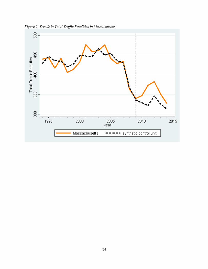
Figure 2 exhibits the trends in total traffic fatalities for Massachusetts and its synthetic
control counterpart from 1994 to 2014. Although there are minor discrepancies, both trends
resemble each other well during the pre-2009 marijuana decriminalization period. In tandem
with the balanced predictor mean values shown in Table 1, Figure 2’s trend line of the synthetic
Massachusetts provides a plausible approximation of the number of total traffic fatalities in
Massachusetts that would have occurred between 2009 and 2014 in the real Massachusetts in the
absence of the 2009 marijuana decriminalization.
The estimation of the effect of 2009 marijuana decriminalization on Massachusetts’ total
traffic fatalities displayed by Figure 2 reveals a noticeable difference right after the
implementation of this policy. Although the number of total traffic fatalities began to rise in
Massachusetts in 2009 until 2013, its synthetic counterpart’s number of total traffic fatalities
continued to decline until 2012. This noticeable discrepancy in total traffic fatalities between the
real Massachusetts and its synthetic counterpart after 2009 suggests a substantial positive effect
of the 2009 marijuana decriminalization policy on the number of total traffic fatalities in
Massachusetts, implying that the policy contributed to an increase in the number of traffic
fatalities in Massachusetts. According to this synthetic control model, Massachusetts’ number of
total traffic fatalities during the period between 2009 and 2014 increased by 150 individuals, or
21
approximately 7.58%, due to the 2009 Massachusetts’ marijuana decriminalization policy.
Although the total number of traffic fatalities in Massachusetts is greater than the total number of
traffic fatalities in the synthetic Massachusetts since 2009, the two trend lines converged by
2014. This suggests that the positive effect of marijuana decriminalization on total traffic
fatalities is likely to be temporary and dissipates after several years.
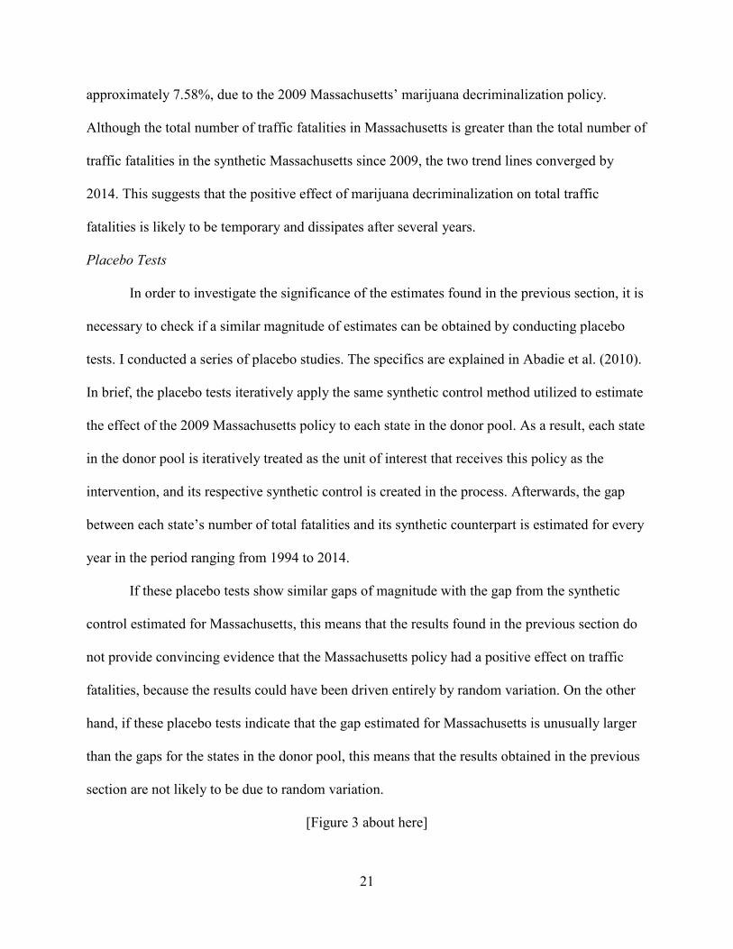
Placebo Tests
In order to investigate the significance of the estimates found in the previous section, it is
necessary to check if a similar magnitude of estimates can be obtained by conducting placebo
tests. I conducted a series of placebo studies. The specifics are explained in Abadie et al. (2010).
In brief, the placebo tests iteratively apply the same synthetic control method utilized to estimate
the effect of the 2009 Massachusetts policy to each state in the donor pool. As a result, each state
in the donor pool is iteratively treated as the unit of interest that receives this policy as the
intervention, and its respective synthetic control is created in the process. Afterwards, the gap
between each state’s number of total fatalities and its synthetic counterpart is estimated for every
year in the period ranging from 1994 to 2014.
If these placebo tests show similar gaps of magnitude with the gap from the synthetic
control estimated for Massachusetts, this means that the results found in the previous section do
not provide convincing evidence that the Massachusetts policy had a positive effect on traffic
fatalities, because the results could have been driven entirely by random variation. On the other
hand, if these placebo tests indicate that the gap estimated for Massachusetts is unusually larger
than the gaps for the states in the donor pool, this means that the results obtained in the previous
section are not likely to be due to random variation.
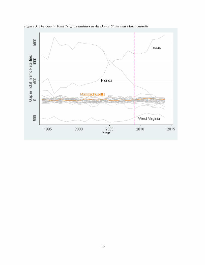
[Figure 3 about here]

22
In total, there are 28 states in the donor pool—Alabama, Arkansas, Delaware, Florida,
Georgia, Hawaii, Iowa, Idaho, Illinois, Indiana, Kansas, Kentucky, Louisiana, Missouri, North
Dakota, New Hampshire, Nevada, Oklahoma, Pennsylvania, South Carolina, South Dakota,
Tennessee, Texas, Utah, Virginia, Wisconsin, West Virginia, and Wyoming. I applied the
synthetic control method to each state to conduct 28 placebo tests. Figure 3 exhibits the results of
these placebo tests. The gray lines denote the gaps in the trends in total traffic fatalities between
each state in the donor pool and its respective synthetic counterpart, while the orange line
represents the gap in total traffic fatalities between Massachusetts and its synthetic counterpart.
As Figure 3 shows, the synthetic Massachusetts has a good fit for total traffic fatalities
prior to the implementation of the 2009 policy along with many other states. For example,
Massachusetts and many donor pool states have lines that stay close to 0 during the pre-
intervention preiod. Although the pre-2009 condition has a mean squared prediction error
(MSPE)—average of the squared differences between traffic fatalities in the real Massachusetts
and its synthetic counterpart from 1994 to 2014—in Massachusetts of 14.67, the pre-2009 policy
median MSPE among the 28 donor states is 43.32, and the mean MSPE is 171.08. This suggests
that a good number of the donor pool states can also produce their synthetic counterpart that has
a relatively good fit for total traffic fatalities prior to the 2009 marijuana decriminalization.
Figure 3 also suggests that the synthetic control method is unable to reproduce the trends in total
traffic fatalities during the period 1994-2008 for some states.
For example, Texas’ pre-2009 MSPE is 1324.44, while Florida’s is 571.37. However,
given that both states’ average total traffic fatalities between 1994 and 2008 are over 3000,
which is far greater than the donor pool’s average 816.77, this does not come as a surprise since
there is no combination of states within the donor pool that can reproduce these states’ trends in
23
total traffic fatalities. Because of the difficulty in visually examining the fit of each state with its
respective synthetic control due to the extreme ouliers—Texas, Florida, and West Virginia in
Figure 3, it is necessary to examine the fit of these other states more closely by dropping these
extreme outliers.
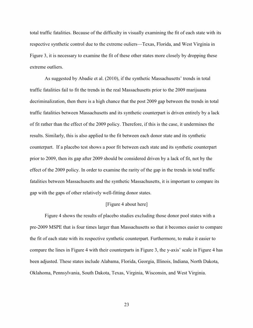
As suggested by Abadie et al. (2010), if the synthetic Massachusetts’ trends in total
traffic fatalities fail to fit the trends in the real Massachusetts prior to the 2009 marijuana
decriminalization, then there is a high chance that the post 2009 gap between the trends in total
traffic fatalities between Massachusetts and its synthetic counterpart is driven entirely by a lack
of fit rather than the effect of the 2009 policy. Therefore, if this is the case, it undermines the
results. Similarly, this is also applied to the fit between each donor state and its synthetic
counterpart. If a placebo test shows a poor fit between each state and its synthetic counterpart
prior to 2009, then its gap after 2009 should be considered driven by a lack of fit, not by the
effect of the 2009 policy. In order to examine the rarity of the gap in the trends in total traffic
fatalities between Massachusetts and the synthetic Massachusetts, it is important to compare its
gap with the gaps of other relatively well-fitting donor states.
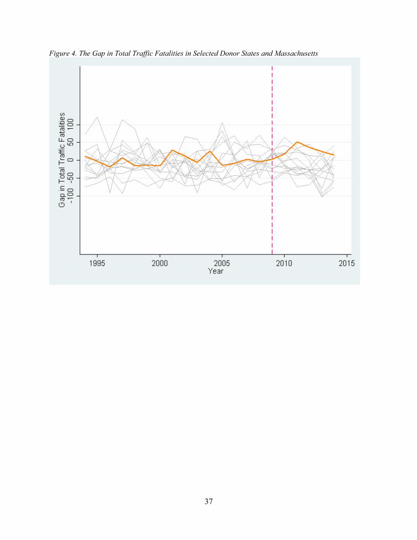
[Figure 4 about here]
Figure 4 shows the results of placebo studies excluding those donor pool states with a
pre-2009 MSPE that is four times larger than Massachusetts so that it becomes easier to compare
the fit of each state with its respective synthetic counterpart. Furthermore, to make it easier to
compare the lines in Figure 4 with their counterparts in Figure 3, the y-axis’ scale in Figure 4 has
been adjusted. These states include Alabama, Florida, Georgia, Illinois, Indiana, North Dakota,
Oklahoma, Pennsylvania, South Dakota, Texas, Virginia, Wisconsin, and West Virginia.
24
Figure 4 includes 14 donor pool state (gray) and Massachusetts (orange). According to
Figure 4, Massachusetts’ post-2009 line is the most unusual line relative to other states; whereas
Massachusetts’ gap line prior to 2009 remains close to 0, it diverges quickly after 2009, making
the gap in the trends in total traffic fatalities between Massachusetts and its synthetic counterpart
the largest relative to other donor pool states during the post-2009 decriminalization period. On
the other hand, a majority of the donor states do not show such a pattern, indicating a poor fit
with their respective synthetic counterpart. Therefore, it is highly likely that the gap for
Massachusetts in the post-2009 condition period is not obtained due to a lack of fit; rather, it is
an evidence of the positive effect of the 2009 policy on total traffic fatalities in Massachusetts.
However, it is still necessary to conduct one more placebo test in order to make sure that the
results for Masscahusetts are not driven entirely by random variation.
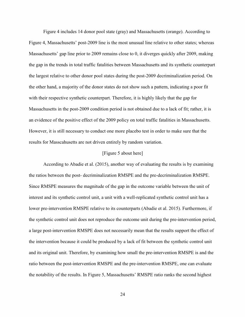
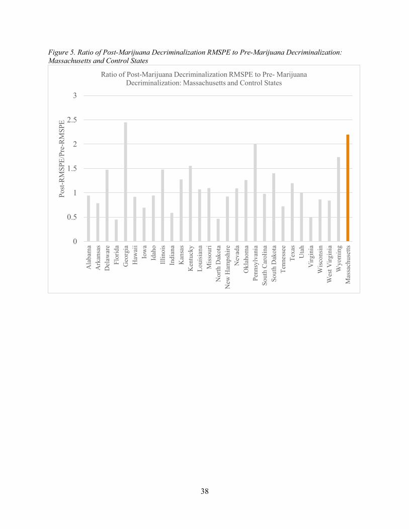
[Figure 5 about here]
According to Abadie et al. (2015), another way of evaluating the results is by examining
the ratios between the post- decriminalization RMSPE and the pre-decriminalization RMSPE.
Since RMSPE measures the magnitude of the gap in the outcome variable between the unit of
interest and its synthetic control unit, a unit with a well-replicated synthetic control unit has a
lower pre-intervention RMSPE relative to its counterparts (Abadie et al. 2015). Furthermore, if
the synthetic control unit does not reproduce the outcome unit during the pre-intervention period,
a large post-intervention RMSPE does not necessarily mean that the results support the effect of
the intervention because it could be produced by a lack of fit between the synthetic control unit
and its original unit. Therefore, by examining how small the pre-intervention RMSPE is and the
ratio between the post-intervention RMSPE and the pre-intervention RMSPE, one can evaluate
the notability of the results. In Figure 5, Massachusetts’ RMSPE ratio ranks the second highest
25
after Georgia. However, given that Massachusetts’s pre-intervention RMSPE is 14.67 while
Georgia’s pre-intervention RMSPE is 63.30, it is clear that Massachusetts’ synthetic control has
a much better fit with the trends in total traffic fatalities of its original unit prior to the 2009
policy compared to Georgia.
DISCUSSION
Recently, the trend of relaxing the restrictions on marijuana possession, and its use, by
decriminalizing marijuana has been gaining strong momentum across the United States.
Currently, it is possible to possess a small amount of marijuana for personal recreational use
without a criminal charge in 21 states (Governing 2017). Despite this strong move toward
decriminalizing marijuana, however, the consequences of this policy are still very much
unknown. For example, what are the implications of implementing this policy on the general
public’s health, on criminal behavior that might be influenced by marijuana use, and on road
safety?
In order to better understand the ramifications of implementing these policies, this study
investigated marijuana decriminalization’s impact on road safety by examining its impact on
traffic fatalities. To my knowledge, there have been no studies investigating the causal effect of
marijuana decriminalization, which affects a larger proportion of the population than medical
marijuana policies, on traffic fatalities. By utilizing the synthetic control method, this study
overcomes the difficulty in finding an appropriate counterfactual. As a result, this research
contributes to the literature by examining the causal impact of marijuana decriminalization
policy on traffic fatalities.
The results of this study provide evidence of a temporary positive effect of the 2009
Massachusetts’ marijuana decriminalization policy on the trend of total traffic fatalities in
26
Massachusetts. In addition, the placebo tests affirm these results by finding that it is highly
unlikely that these effects are due to random variability. Although the impact of the 2009
Massachusetts policy appeared to increase fatalities from 2009 until 2012, the effect has begun to
dissipate since 2012, and the gap between the trends in total fatalities between Massachusetts and
its synthetic counterpart became almost non-existent by 2014.
The results of this study may help explain why previous studies on marijuana policy
changes have found divergent outcomes. Brady and Li (2014) found that marijuana was the most
commonly detected illicit drug among drivers involved in traffic fatalities from their study of the
U.S. FARS data, suggesting that an increase in marijuana use and its availability is likely to
increase the number of traffic fatalities. On the other hand, both Anderson et al.’s (2011) study
and Anderson and Ree’s (2014) study discovered a statistically significant negative association
between medical marijuana availability and traffic fatalities. As discussed, the results from this
study show an increase in the number of total traffic fatalities in Massachusetts compared to its
synthetic counterpart in 2009 but a decline in the total traffic fatalities in Massachusetts since
2012, with the gap in the traffic fatalities in both units almost non-existent in 2014. This provides
a potential explanation of these variable findings: the effect of changes in marijuana policy may
be temporary and dissipate once the norms surrounding licit marijuana develop.
However, the findings from this study need to be taken with caution. Although the
results indicate a temporary positive effect of marijuana decriminalization on traffic fatalities,
this may not be the case in other states or countries that are highly divergent with Massachusetts
in both their observable and unobservable characteristics. However, given that Massachusetts is
a relatively mid-sized state that is not too divergent from a majority of the states within the U.S.,
I argue that this relationship is likely to be generalizable to a majority of states within the U.S.
27
This paper signifies the need for future studies investigating the causal association
between marijuana decriminalization and traffic fatalities to see if the relationship found in
Massachusetts still holds to be true in other parts of the U.S. or the world. Furthermore, in order
to deepen the understanding of the impact of marijuana decriminalization, future studies should
consider investigating the heterogenous effects of marijuana decriminalization on traffic fatalities
based on age groups, gender, and residential density since this study does not investigate the
potential heterogeneous effects of marijuana decriminalization on traffic fatalities. Moreover,
researchers should investigate whether the decline in the total traffic fatalities since 2012 in
Massachusetts compared to its synthetic counterpart was caused by any events or policies in
Massachusetts that I failed to account for in the synthetic control model used in this study, in
order to understand the causes of this phenomenon. Finally, studies investigating why marijuana
decriminalization is associated with an increase in traffic fatalities are needed in order to better
understand the causal mechanism between marijuana decriminalization and traffic fatalities.
The findings from this study suggest that states considering decriminalizing marijuana
should be prepared for the increased danger on their roads before implementing such policies.
This study suggests that there is a causal association between marijuana decriminalization and
traffic fatalities, albeit temporary. Preparing for this initial increase in the roads danger by
implementing specific policies, such as increasing the number of traffic patrols, enacting strict
laws punishing drivers driving under the influence of marijuana, and educating residents about
the danger of driving under the influence of marijuana, is likely to prevent potential traffic
accidents that would otherwise be likely to occur.
28
REFERENCES
Abadie, Alberto, Alexis Diamond, and Jens Hainmueller. 2010. “Synthetic Control Methods for
Comparative Case Studies: Estimating the Effect of California’s Tobacco Control
Program.” Journal of the American Statistical Association 105(490):493-505.
Abadie, Alberto, Alexis Diamond, and Jens Hainmueller. 2015. “Comparative Politics and the
Synthetic Control Method.” American Journal of Political Science 59(2):495-510.
Anderson, Mark D., Benjamin Hansen, and Daniel I. Rees. 2011. “Medical Marijuana Laws,
Traffic Fatalities, and Alcohol Consumption.” Journal of Law and Economics 56(2):333-
369.
Anderson, Mark D., and Daniel I. Rees. 2014. “The Legalization of Recreational Marijuana:
How Likely Is the Worst‐Case Scenario?” Journal of Policy Analysis and
Management 33(1):221-232.
Bijleveld, Frits, Jacques Commandeur, Phillip Gould, and Siem Jan Koopman. 2008. “Model-
Based Measurement of Latent Risk in Time Series with Applications. Journal of the
Royal Statistical Society 171(1):265-277.
Brady, Joanne E., and Guohua Li. 2014. “Trends in Alcohol and Other Drugs Detected in Fatally
Injured Drivers in the United States, 1999–2010.” American Journal of Epidemiology
179(6):692-699.
Cameron, Lisa, and Jenny Williams. 2001. “Cannabis, Alcohol and Cigarettes: Substitutes or
Complements?” Economic Record 77(236):19-34.
DeAngelo, Gregory, and Benjamin Hansen. 2014. "Life and Death in the Fast Lane: Police
Enforcement and Traffic Fatalities." American Economic Journal: Economic
Policy 6(2):231-257.
29
Hardaway, Robert. M. 2003. No Price Too High: Victimless Crimes and the Ninth Amendment.
Westport, CT: Greenwood Publishing Group.
GOVERNING. 2017. “State Marijuana Laws in 2017 Map.” Retrieved April 12, 2017
(http://www.governing.com/gov-data/state-marijuana-laws-map-medical-
recreational.html).
Halsey, Ashley. 2016. “Unlike Alcohol, It’s Tough to Set DUI Limits for Marijuana.” The
Washington Post, May 10.
Davis, Joshua C. 2015. “The business of Getting High: Head Shops, Countercultural Capitalism,
and the Marijuana Legalization Movement.” The Sixties 8(1):27-49.
Nghiem, Son, Jacques Commandeur, and Luke B. Connelly. 2016. “Determinants of Road
Traffic Safety: New Evidence from Australia Using State-Space Analysis.” Accident
Analysis and Prevention 94(1):65-72.
Marijuana Policy Project. 2017. “Massachusetts: Defending Question 4.” Retrieved April 23,
2017 (https://www.mpp.org/states/massachusetts/).
Miech, Richard A., Lloyd Johnston, Patrick M. O’Malley, Jerald G. Bachman, John
Schulenberg, and Megan E. Patrick. 2015. “Trends in Use of Marijuana and Attitudes
Toward Marijuana among Youth Before and After Decriminalization: The Case of
California 2007–2013.” International Journal of Drug Policy 26(4):336-344.
NORML. 2017. “States That Have Decriminalized.” Retrieved April 24, 2017
(http://norml.org/aboutmarijuana/item/states-that-have-decriminalized).
Oksanen, Atte, Mikko Aaltonen, and Janne Kivivuori. 2014. “Driving Under the Influence as a
Turning Point? A Register‐Based Study on Financial and Social Consequences among
First‐Time Male Offenders.” Addiction 110(3):471-478.
30
O’Malley, Patrick M., and Lloyd Johnston. 2007. “Drugs and Driving by American High School
Seniors, 2001–2006.” American Journal of Public Health 68(6):834-842.
Pacula, Rosalie L., Jamie F. Chriqui, and Joanna King. 2003. “Marijuana Decriminalization:
What Does It Mean in the United States?” National Bureau of Economic Research.
Retrieved April 24, 2017 (http://www.nber.org/papers/w9690).
Pacula, Rosalie L. 1998. “Does Increasing the Beer Tax Reduce Marijuana Consumption?”
Journal of Health Economics 17(5):557-585.
Pew Research Center. 2016. “Support for Marijuana Legalization Continues to Rise.” Retrieved
April 12, 2017 (http://www.pewresearch.org/fact-tank/2016/10/12/support-for-marijuana-
legalization-continues-to-rise/).
Pratt, Stephanie. 2003. "Work-Related Roadway Crashes: Challenges and Opportunities for
Prevention.” NIOSH Hazard Review. Retrieved April 24, 2017
(https://www.cdc.gov/niosh/docs/2003-119/pdfs/2003-119.pdf).
Roberts, Chris. 2017. “How to Beat a Marijuana DUI.” High Times, January 4.
Salsberg, Bob. 2016. “Voters in Massachusetts Approve Legalizing Recreational Marijuana.”
The Boston Globe, November 9.
Santaella-Tenorio, Julian, Christine M. Mauro, Melanie M. Wall, June H. Kim, Magdalena
Cerdá, Katherine M. Keyes, Deborah S. Hasin, Sandro Galea, and Silvia S. Martins.
2017. “US Traffic Fatalities, 1985–2014, and Their Relationship to Medical Marijuana
Laws.” American Journal of Public Health 107(2):336-342.
Schrader, Megan. 2015. “Colorado Legislators Working to Draft Drugged Driving Bill.” The
Gazette, July 25.
31
Thies, Clifford F., and Charles A. Register. 1993. “Decriminalization of Marijuana and the
Demand for Alcohol, Marijuana and Cocaine.” The Social Science Journal 30(4):385-
399.
Zhao, Xueyan, and Mark N. Harris. 2004. “Demand for Marijuana, Alcohol and Tobacco:
Participation, Levels of Consumption and Cross-equation Correlations.” Economic
Record 80(251):394-410.
32
TABLES
Table 1. Total Traffic Fatalities Predictor Means for the Pre-intervention Period (1994-2008) Variables Massachusetts Synthetic
Control Donor States
Total Traffic Fatalities(1994) 440 428.72 819.87
Total Traffic Fatalities(1999) 414 427.34 875.11
Total Traffic Fatalities(2004) 476 449.74 901.29
Total Traffic Fatalities(2008) 364 367.52 801.86
Licensed Driver Ratio 72.09 68.96 69.96
Poverty Ratio 10.43 10.41 12.15
Labor Force Ratio 67.73 67.63 67.26
ln Residents 15.65 14.50 14.99
Law Enforcement Officers 263.10 256.35 229.01
ln Total Past Month Marijuana Use 13.57 13.29 13.15
ln Total Past Month Alcohol Use 15.60 15.43 15.36
ln real GDP per capita 10.87 10.77 10.61
Unemployment Ratio 4.56 4.55 4.63
Registered Motor Vehicle Ratio 82.10 80.26 85.92
Employment Ratio 64.63 64.57 64.18
All Variables except Total Traffic Fatalities(1994, 1999, 2004, 2008), Law Enforcement Officers (1999-2008), ln Total Past Month Marijuana Use (1999-2008), ln Total Past Month Alcohol Use (1999-2008), are averaged for the period 1994-2008.

33
Table 2. Synthetic Control Weights State Weight State Weight
Alabama Montana
Alaska Nebraska
Arizona Nevada
Arkansas New Hampshire .067
California New Jersey
Colorado New Mexico
Connecticut New York
Delaware .273 North Carolina
Florida North Dakota
Georgia Ohio
Hawaii .25 Oklahoma
Idaho Oregon
Illinois .091 Pennsylvania .001
Indiana Rhode Island
Iowa South Carolina
Kansas South Dakota
Kentucky Tennessee
Louisiana .069 Texas
Maine Utah
Maryland Vermont
Massachusetts Virginia .001
Michigan Washington
Minnesota West Virginia .05
Mississippi Wisconsin .197
Missouri Wyoming

34
FIGURES
Figure 1. Trends in Total Traffic Fatalities in Massachusetts, the Donor States Average, and the USA Average
35
Figure 2. Trends in Total Traffic Fatalities in Massachusetts
36
Figure 3. The Gap in Total Traffic Fatalities in All Donor States and Massachusetts
37
Figure 4. The Gap in Total Traffic Fatalities in Selected Donor States and Massachusetts
38
Figure 5. Ratio of Post-Marijuana Decriminalization RMSPE to Pre-Marijuana Decriminalization: Massachusetts and Control States
0
0.5
1
1.5
2
2.5
3A
laba
ma
Ark
ansa
sD
elaw
are
Flor
ida
Geo
rgia
Haw
aii
Iow
aId
aho
Illin
ois
Indi
ana
Kan
sas
Ken
tuck
yLo
uisi
ana
Mis
sour
iN
orth
Dak
ota
New
Ham
pshi
reN
evad
aO
klah
oma
Penn
sylv
ania
Sout
h C
arol
ina
Sout
h D
akot
aTe
nnes
see
Texa
sU
tah
Virg
inia
Wis
cons
inW
est V
irgin
iaW
yom
ing
Mas
sach
uset
ts
Post
-RM
SPE/
Pre-
RM
SPE
Ratio of Post-Marijuana Decriminalization RMSPE to Pre- Marijuana Decriminalization: Massachusetts and Control States
39
APPENDIX
In this appendix, I describe the specific sources of the data used in this study. All the data
used for the analysis are state-level, longitudinal data ranging from 1994 to 2014 unless they are
specified.
• The number of total traffic fatalities. Source: The Fatality Analysis Reporting System
(FARS).
• Licensed Drivers Ratio: Highway Statistics maintained by the Federal Highway Association.
• Registered Motor Vehicle Ratio: The Fatality Analysis Reporting System (FARS).
• Log Residents: The Fatality Analysis Reporting System (FARS).
• Law Enforcement Officers: The Federal Bureau of Investigation’s the Uniform Crime
Reports data.
• Log Marijuana use in the past 30 days. Source: The National Household Survey on Drug
Abuse (NHSDA) and the National Survey of Drug Use and Health (NSDUH). These data
were available from 1999 through 2014.
• Log Real per capita GDP. Source: Bureau of Economic Analysis
• Poverty ratio. Source: U.S. Bureau of the Census.
• Unemployment rate. Source: Bureau of Labor Statistics.
• Employment rate: Source: Bureau of Labor Statistics.
• Marijuana decriminalization. Source: the data were gathered by examining each state’s
legislature’s website and by comparing with the information on norml.org.
• Medical marijuana decriminalization: the data were gathered by examining each state’s
legislature’s website and by comparing with the information on norml.org.
40
• Recreational marijuana legalization: the data were gathered by examining each state’s
legislature’s website and by comparing with the information on norml.org.
• Log Alcohol consumption per capita: The National Household Survey on Drug Abuse
(NHSDA) and the National Survey of Drug Use and Health (NSDUH). These data were
available from 1999 through 2014.


![+ 2 (,1 1/,1(...2015/07/01 · 2016] DECRIMINALIZATION AND PRIVATIZATION 5 enforcement patterns for traffic violations and marijuana offenses as well as the hotly contested benefits](https://img.pdfslide.net/doc/110x75/5fe73e81ef4aaf7ee233530d/-2-1-11-20150701-2016-decriminalization-and-privatization-5-enforcement.jpg)