Does Money Impede Convergence? - Luiss Guido Carlistatic.luiss.it/RePEc/pdf/cesare/1501.pdf · comparable. _ Lucas (1980), like Barro and Grossman (1971), models an economy with two

1

Does Money Impede Convergence?

John D Hey1 and Daniela Di Cagno2

Abstract Inspired by Clower’s conjecture that the necessity of trading through money in monetised economies might hinder convergence to competitive equilibrium, and hence, for example, cause unemployment, we experimentally investigate behaviour in markets where trading has to be done through money. In order to evaluate the properties of these markets, we compare their behaviour to behaviour in markets without money, where money cannot intervene. As the trading mechanism might be a compounding factor, we investigate two kinds of market mechanism: the double auction, where bids, asks and trades take place in continuous time throughout a trading period; and the clearing house, where bids and asks are placed once in a trading period, and which are then cleared by an aggregating device. We thus have four treatments, the pairwise combinations of non-monetised/monetised trading with double auction/clearing house. We find that: convergence is faster under non-monetised trading, implying that the necessity of using money to facilitate trade hinders convergence; that monetised trading is noisier than non-monetised trading; and that the volume of trade and realised surpluses are higher with the double auction than the clearing house. As far as efficiency is concerned, monetised trading lowers both informational and allocational efficiency, and while the double auction outperforms the clearing house in terms of allocational efficiency, the clearing house is marginally better than the double auction in terms of informational efficiency when trade is through money. Crucially we confirm the conjecture that inspired these experiments: that the necessity to use money in trading hinders convergence to competitive equilibrium, lowers realised trades and surpluses, and hence may cause unemployment. JEL Classifications: C92, D40, E24 Keywords: clearing house mechanism, double auction mechanism, experimental markets, money, monetised trading, non-monetised trading. Acknowledgements: The authors would like to express their gratitude to Andrea Lombardo for writing the software in Visual Studio for these experiments. We also thank LUISS for use of their purpose-built laboratory, run under the auspices of CESARE. Finally we would like to thank the Editor and three referees for invaluable comments which led to significant changes in the paper. Corresponding author: Hey, Department of Economics and Related Studies, University of York, Heslington, York YO10 5DD, UK, [email protected]

1 University of York, UK

2 LUISS, Rome, Italy

mailto:[email protected]

2

1. Introduction

As Clower famously said in 1967, as part of the then on-going ‘Keynesian Revolution’ (partly initiated

by Leijonhufvud, 1968): “Money buys goods and goods buy money; but goods do not buy goods”.

This aphorism seemed to have been forgotten as part of the demise of Keynes’ ideas, but is now

coming back into economists’ thoughts as a consequence of recent events. The key idea is that, in

money-based economies, goods cannot be bartered directly for each other; instead money has to be

used as a go-between. This may interfere with convergence to equilibrium, particularly, as Clower

thought, in the labour market: firms do not employ workers as they cannot see the extra sales

generated by them doing so. Involuntary unemployment may result.

In Hey and Di Cagno (1998) we reported on an experiment to test Clower’s conjecture, using a

monetised trading market with the double auction trading mechanism. We did indeed see a

departure from convergence to the competitive equilibrium, but that experiment was partial in that

it did not compare the monetised trading outcome with the non-monetised trading outcome. Other

factors may have been influencing our results.

One possibility is that the results may have been the consequence of the objective function imposed

on our subjects (that of a utility function rather than through the use of reservation prices). Indeed

our objective function (maximising a function of two variables, rather than simply maximising

surplus as is usually the case) may be perceived as being more complicated for subjects to

understand, and it may have been that, rather than having to trade through money, that caused the

lack of convergence.

Moreover we felt that the lack of convergence might have resulted from the trading mechanism that

we used, rather than from the trading through money. While, as we note later, there is a general

acceptance that the double auction mechanism is robustly efficient, there are studies that show

greater efficiency with other mechanisms. For example, Goeree and Lindsay (2012b) show that with

what they call a ‘schedule market’ – in which subjects enter effectively a demand schedule –

efficiency reaches 95% while with a parallel double auction market it reaches only 77%. So we

3

implemented additional treatments with a second mechanism – that of the clearing house3 – in

which subjects enter effectively a (price,quantity) pair which are then aggregated to clear the market

by the experimenter. Hence the present experiment, in which we have four treatments, with each of

non-monetised trading and monetised trading paired with each of two trading mechanisms – double

auction and clearing house. We shall see that our conjecture about the two market mechanisms is

not confirmed by the evidence; on the other hand Clower’s conjecture is – for both mechanisms.

The paper is organised as follows: in section 2, we outline Clower’s conjecture and the theoretical

literature that explored his conjecture; in section 3, we discuss the issues of efficiency in markets; in

section 4, we describe our experimental design; in section 5, we describe our results. Section 6

concludes.

2. Clower’s conjecture and subsequent theoretical literature

Clower’s conjecture was simple and intuitively appealing – the necessity of monetised trading might

cause a lack of convergence to the competitive equilibrium. The publication of his paper sparked off

a flurry of theoretical work aimed at investigating his conjecture. There is one clear and repeated

conclusion from this literature: that convergence to the competitive equilibrium might not be

attained. Moreover, there might be several possible equilibria, and expectations might be important.

The various theoretical contributions differ in their assumptions about the market and about

trading. We cannot cover all the contributions, and so concentrate on those that are relevant for our

experimental design. This was as follows (we give more detail later): we had two goods in our

experiment and two kinds of agents, both of which started trading with stocks of just one of the two

goods. They are motivated to trade through a payoff function, which is a Cobb-Douglas function

defined over the amounts of the two goods that they hold at the end of trading. In the monetised

treatments they had to trade through money – which is worthless at the end of the experiment.

3 We note that this is not the same as Goeree and Lindsay’s (2102b) schedule market, though it does have

some features in common.

4

Because of this feature, and to facilitate trade, we implemented a random stopping mechanism, for

otherwise subjects might backwardly induct with, as a consequence, no trade resulting.

One of the earlier papers that followed up Clower’s conjecture was that of Barro and Grossman

(1971) which adopted a framework similar to ours, in that there are two goods (‘labor services’ and

‘consumable commodities’) and money. However for most of the analysis prices are fixed and the

process of adjustment is not considered. They use the expression ‘disequilibrium’, though this

should be considered as equilibrium with fixed prices. Similarly Benassy (1975) talks about Neo-

Keynesian Equilibrium (or K-equilibrium) – though once again prices are fixed – finding the existence

of some equilibria where the level of trade and economic activity are depressed because of the

wrong exchange rate. Both these papers have centralised trading. In contrast, Kiyotaki and Wright

(1989) talk about equilibria with random matching and conclude that the “equilibria are not

generally Pareto optimal and that when multiple equilibria coexist they are not generally Pareto

comparable.” Lucas (1980), like Barro and Grossman (1971), models an economy with two goods

and money, but with uncertainty (here about preferences). He concludes that “the monetary

equilibrium … will not be efficient.” Ostroy and Starr (1974) start with a barter economy and then

introduce money. They conclude that “in the absence of double coincidence such a trading rule [one

essentially satisfying double coincidence of wants] will achieve an inefficient allocation far from

competitive equilibrium”. Moreover, they assert that in barter settings there exist no “plausible”

trading rules (that is, rules which place limits on the ingenuity or computational capacity of traders).

Shapley and Shubik (1977) adopt a game-theoretic analysis and consider the various possible non-

cooperative equilibria. They conclude that “a striking feature of this kind of equilibrium is its non-

optimality”. This result is echoed throughout this literature.

Some recent papers consider the adjustment process of prices in this kind of framework; so their

analyses are dynamic. Of particular relevance are the papers by Crockett et al (2011), Gjerstad

(2013) and Goeree and Lindsay (2012a and 2012b). We are primarily interested in the differences

between the four treatments, but dynamics obviously play a role since trading is repeated over a

5

random number of trading days. If the price adjustment process is unstable, then we have to be

careful about interpreting our results. We will have more to say about this later.

3. Efficiency and market mechanisms

We implement two different market mechanisms: the double auction and the clearing house. We

wanted to see if the deterioration moving from non-monetised trading to monetised trading was a

special feature of the double auction. But first we must define what we mean by ‘deterioration’.

Here we are referring to efficiency. There are several definitions of market efficiency, but we

concentrate on two: informational efficiency and allocational efficiency. The former concerns

convergence to the competitive price, and the latter refers to the realised gains from trade.

Friedman (1993) provides an early experimental study comparing the double auction and the

clearing house, though in the context of non-monetised trading. He concludes that “clearinghouse

markets are as informationally efficient as double auction markets and almost as allocationally

efficient”, while Cason and Friedman (2008) summarise a wealth of experimental evidence by

saying that “price deviations from competitive equilibrium tend to be the smallest with the SCM

[clearing house], while volume is highest in CDA [double auction]”. As we have already noted these

results pertain to non-monetised trading. We are interested in seeing whether they carry over to

monetised trading.

Our focus on different market mechanisms and trading rules is also relevant for policy concerns

since actual financial markets are organized in such a way that can be interpreted as that both non-

monetised trading and monetised trading may occur (that is, the Tokyo Stock Exchange opens when

New York closes). Moreover, we can find examples of markets which use a clearing house

mechanism – such as the MTS Electronic Government Bond market – whereas Stock Exchanges

generally implement a double auction mechanism.

6

4. The Experiment

We now give more detail on the experimental design. The environment is as simple as possible, yet

staying faithful to Clower’s insight. There are two goods, X and Y. There are two types of traders:

Type X and Type Y and there are n of each type4. Trading is divided up into trading days. In each day,

Type X traders are endowed with a quantity x of Good X, but none of Good Y; mutatis mutandis Type

Y traders are endowed with none of Good X but a quantity y of Good Y. Trade takes place through

the day and the payment to each subject depends upon the amounts of the two goods they end up

with at the end of the day. To be specific if a trader of either type ends the day with x of Good X and

y of Good Y their payment for that day will be 10√(xy) in euro cents5. Clearly if either type of agent

does not trade in any day, they end up with zero payment for that day. Goods cannot be carried over

from day to day.

We had four treatments, namely each of non-monetised trading and monetised trading paired with

each of double auction and clearing house. We had three sessions of each treatment (with different

parameters – see later), each duplicated – giving a total of 24 sessions. We use the following

notation (where the i = 1,2,3 refers to a particular session of that treatment):

double auction (D) clearing house (C)

non-monetised trading (N) NDi NCi

monetised trading (M) MDi MCi

In the non-monetised treatments, each trading day is independent of all the others and there is no

money. In the monetised treatments, however, there is (experimental) money and trade must be

carried out using this (experimental) money. Accordingly, in the monetised treatments, we divided

up each trading day into a morning, an afternoon and an evening: in the morning the market for

Good X was open and agents could buy and sell Good X using (experimental) money; in the

afternoon the market for Good Y was open and agents could buy and sell Good Y using

4 In the experiment we put n equal to 5. We deliberately made the numbers of each type the same, and made

the total number of subjects in each session sufficiently high to avoid any monopolistic possibilities. 5 The experiment was conducted in Italy and subjects were paid in euros. There are 100 centesimi in a euro. A

euro is currently worth about £0.74 or $1.13.

7

(experimental) money; in the evening accounting was done and the agents informed as to how much

real money they had earned for that day. The experimental money used in the trading process had

no value, however; all agents were endowed with a stock of experimental money at the beginning of

the experimental session but it was worthless at the end.

There is a potential problem here however: if the subjects knew the number of trading days that the

experiment would last, and if they could perform backward induction, no trade would ever take

place. Since experimental money is worthless at the end of the experiment, no Type Y would want to

accept any experimental money on the afternoon of the final day; as a consequence no Type X

would accept any money in the morning of the final day, and so on backwards. To solve this

problem, we made the number of days that the experiment lasted random. Ideally we would have

preferred to have had a stationary mechanism so that the probability of any day being the final day,

given that the experiment had lasted to that day, would be a fixed number, but there are two

problems with this: first, subjects seem to have difficulty in understanding the mechanism (if we say

the probability of the experiment finishing at the end of any day is 0.1, they get increasingly nervous

at and after day 10, even though there is no need to be); second if we implement it honestly, we

could end up with a session having very few days, thus giving us very few observations. We adopted

a compromise: we said that the experiment would last at least 18 days, and that then and thereafter

the probability would be one-half that the experiment would finish at the end of any day. In practice,

13 of the 24 sessions lasted 18 periods, 9 lasted 19 periods and 2 lasted 20 periods.

As we have already noted, we ran three different sessions of each treatment, each duplicated. These

differed in terms of the x and y. Specifically, in sessions i = 1, x = y = 40; in sessions i = 2, x = 60 and y

= 30; and in sessions i = 3, x = 30 and y = 60. In some of the data analysis that follows we aggregate

the data for the duplicated three sessions for each treatment.

Now let us investigate the stationary equilibrium implied by this setup. We consider each day as a

whole. Let us denote by p and q the (absolute) prices of Good X and Good Y. Type X subjects want to

maximise 10√(xy) subject to px = px + qy; the solution to this is x* = x/2 and y* = (px)/(2q). Type Y

8

subjects want to maximise 10√(xy) subject to qy = px + qy; the solution to this is x* = (qy)/(2p) and y*

= y/2. Given that there are equal numbers of each type, equilibrium implies that, (px)/(2q) = y/2, and

x/2 = (qy)/(2p), and hence that the relative price of Good Y in the stationary equilibrium, q/p, is

equal to x/y. Thus the good relatively lower in supply is relatively higher priced. In our three

sessions, this stationary equilibrium relative price of Good Y is 1 in sessions 1, 2 in sessions 2, and 0.5

in sessions 3. Our experiment is partly to see if actual relative prices converge to these. We note that

in this static competitive equilibrium, the payment to any subject on any given day is given by 5√(x

y).

One might also be interested in a dynamic equilibrium, if the experiment is considered as dynamic6.

Clearly, in such an equilibrium, both types of agent have to end each day with the same amount of

money as they started (for otherwise one Type would be increasing their stock at the expense of the

other). Now consider a subject of Type X, starting each day with an amount x of Good X (the same

analysis, mutatis mutandis, applies to the Type Y). Let us denote by Vt(x) the total expected earnings

for such a subject over the lifetime of the experiment as viewed from period t. Then we have that

Vt(x) = max{10√(xy) + (1-p)Vt+1(x) + p0} subject to px = px + qy (since when the experiment finishes no

further earnings are possible). It follows that if Vt(x) = V(x) for all t, then V(x) = max{10√(xy)/p}

subject to px = px + qy, and hence we get the same objective function as in the one-shot problem –

and the solution is identical. The random stopping mechanism makes no difference to this

equilibrium, though there may well be others.

We now give some practical detail. The experiment was carried out in the purpose-built CESARE7

laboratory at LUISS in Rome. It was run using software written in Visual Studio by Andrea Lombardo.

Subjects were recruited from a register using ORSEE (Greiner 2004). Instructions were in Italian; an

English translation can be found in the Appendix (not to be published) and online where there is

further detail. The software included a calculator which enables subjects to see the real money

6 In a sense it is a repeated, rather than a dynamic, problem, except for the existence of – ultimately worthless

– experimental money. 7 CEntro Sperimentale A Roma Est.

http://www.york.ac.uk/economics/research/centres/experimental-economics/research/unpublishedpapers/#tab-2

http://static.luiss.it/hey/cesare/index.htm

9

earnings for any end-of-day holdings of the two goods. There were a total of 24 sessions, 6 of each

treatment, with 10 subjects in each session. In any one treatment, all parameters were fixed. No

communication was allowed between the subjects. After subjects arrived they were given written

instructions and any questions were answered. Subjects were aware only of their endowments of

the two goods and not the endowments of the other subjects in the experimental session. The

experiment then started and continued until the computer randomly determined when it was over.

Subjects were paid in cash and, after signing a receipt, were free to go. No subject participated in

more than one session. Subjects earned on average €31.03. Different treatments lasted different

amounts of time, with the monetised treatments taking longer.

A brief comment should be made about the calculation of the clearing price in the non-monetised

clearing house treatment, as it differs from the usual case where trading is with money. In the usual

context all buyers state a (price, quantity) pair; sellers likewise. These are aggregated into step

functions in (price, quantity) space and a market-clearing price found where the step functions

intersect. However, in our setup, where we have two goods, the mechanism is somewhat different:

buyers state a (quantity of X, quantity of Y) pair and sellers’ do likewise. The meaning is as follows. If

a buyer’s pair is (x,y) this means that he/she is willing to exchange up to x units of X in exchange for

at least y units of Y. The same applies, mutatis mutandis, for the sellers. How do we find the

equilibrium relative price? We cannot use step functions as neither good is money and we want to

find an equilibrium relative price of Y (or of X – which is the inverse). For example if 2 units of X are

exchanged for 3 units of Y, then the relative price of Y is 2/3 or the relative price of X is 3/2. How do

we find this? There are two ways – which give the same answer. The first is to draw a graph with the

quantity of X along the horizontal axis and the relative price of X on the vertical axis. In this space the

supply curve is the usual kind of step function, but the demand function is different: between the

horizontal steps the demand curve takes the form of a rectangular hyperbola. The same is true,

mutatis mutandis, if one does the analysis with the quantity of Y on the horizontal axis and the

relative price of Y on the vertical axis. With either analysis one finds the relative price of X (or of Y –

10

its inverse) and the quantities of the two goods exchanged in equilibrium. Of course, we did not

explain, or need to explain, this to the subjects, though we did show them a graph of the implied

demand and supply functions.

5. Results

5.1 Prices and Volumes

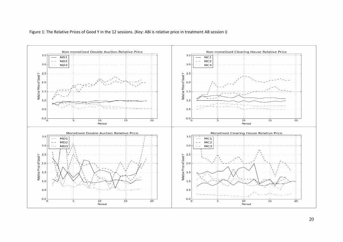
The key results concerning the pattern of prices during the periods of the experiment can be found

in Figure 1. We should note that for each treatment and each session, there are two lines,

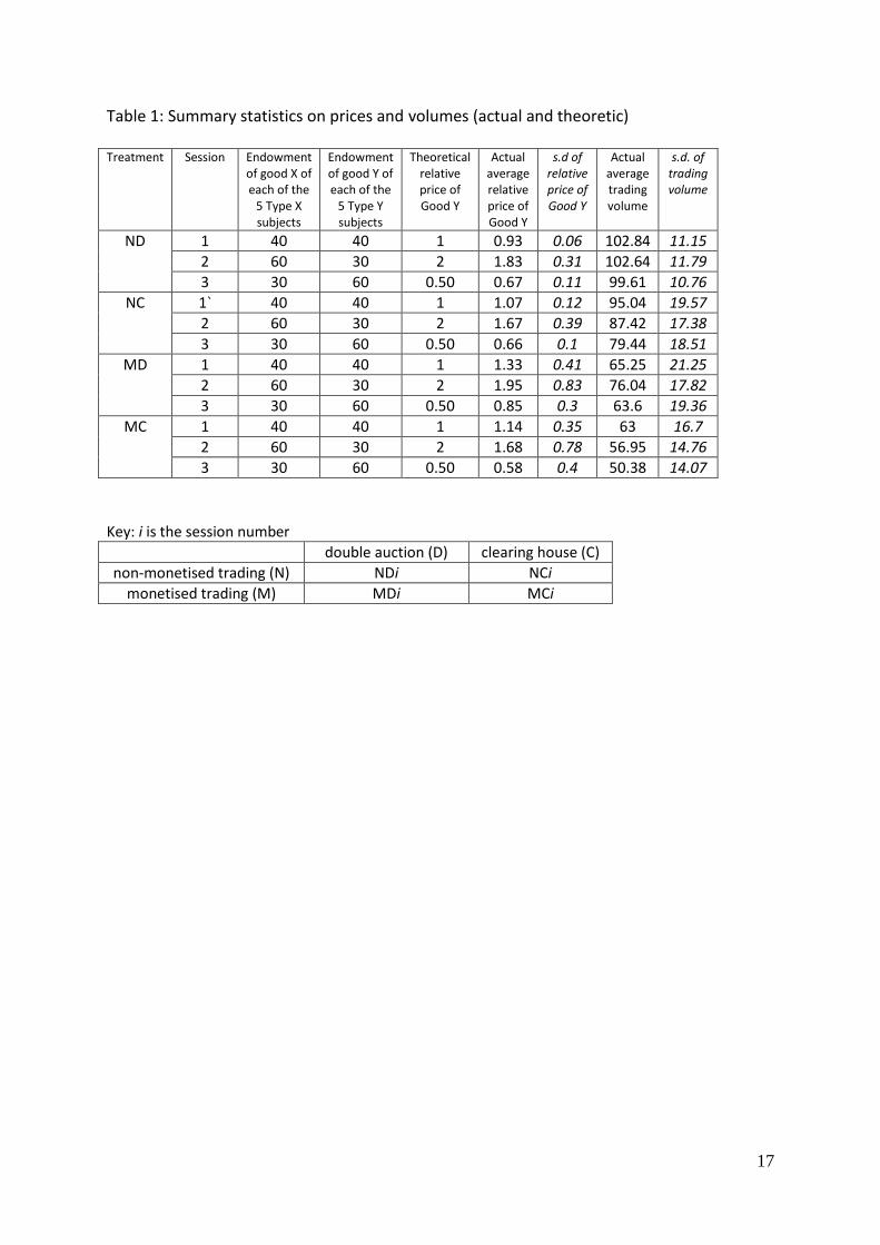
corresponding to the duplicated sessions. Overall means and standard deviations can be found in

Table 1. If we start with the conventional treatment – the non-monetised double auction, ND – we

see from the top left hand graph that the relative price of Good Y converges rapidly to the

theoretical predictions (1 for ND1, 2 for ND2 and 0.5 for ND3). The first of these is particularly rapid,

but this may be because of some kind of focal point effect (equality of prices). This may also account

for the initial stages of ND2 and ND3 – starting off around 1 before almost converging to their

theoretical values; ND3 is slightly high at the end. The non-monetised clearing house, NC, in the top-

right, is almost as good, though here one of the NC2 sessions is slightly above and one slightly below

its theoretical value, while one of the NC3 is also above its theoretical value.

When we get on to the monetised sessions, things change. The bottom-lower graph in Figure 1

shows that prices are erratic, particularly for MD1. The mean price in MD1 is in between the mean

price in MD2 and MD3, as it should be, but the mean prices in MD2 and MD3 are somewhat away

from their theoretical values, and the variances are high – indicating that the trading through money

is hindering convergence to equilibrium. Interestingly the monetised clearing house (in the bottom-

right) is somewhat less erratic and the average price in MC1 is close to its theoretical value, while in

MC2 the relative price of Good Y is below what it should be and in MC3 it is slightly above.

We suspect that the sharp upturn in the relative price of Good Y in the monetised double auction

may have been a consequence of subjects getting apprehensive about the end of the experiment,

11

and, in particular, with Type Y subjects getting increasingly reluctant to sell (in exchange for probably

worthless experimental money).

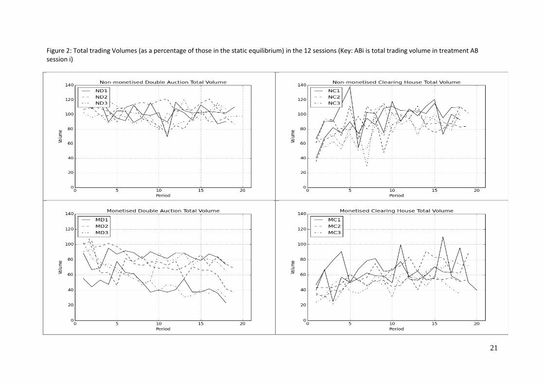
One feature that we would expect from prices being away from equilibrium is that trading volumes

are different from those that we would expect. Figure 2 shows total trading volumes, expressed as a

percentage of the volume in the static competitive equilibrium. Means and standard deviations are,

once again, shown in Table 1. We should note that there is no reason why this measure might not be

above 100% - if there is ‘too much’ trade.

Looking at Figure 2, we see that in the non-monetised double auction treatment, volumes are

generally close to 100%. The same is true for the non-monetised clearing house, though it takes

somewhat longer to get close to 100%. Things change dramatically, though, with the monetised

treatments, where trading volumes are well below 100%, both for the double auction and the

clearing house, though the latter is more erratic.

5.2 Dynamics

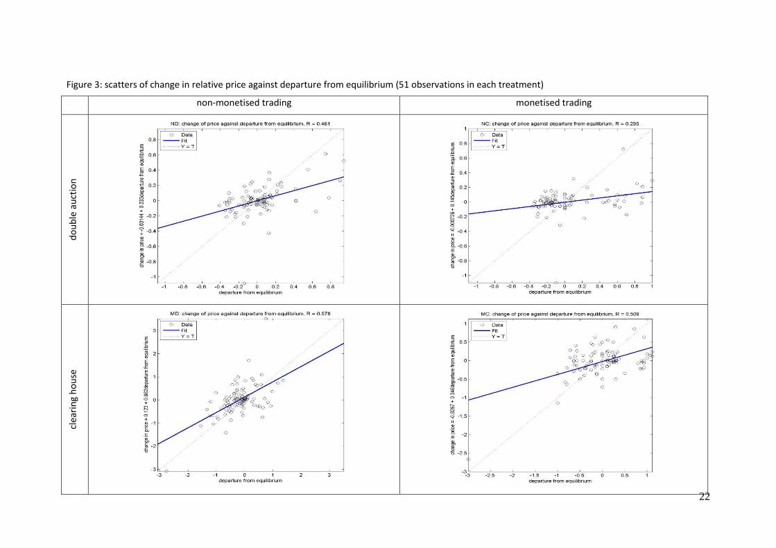
In order to shed some light on the dynamics of the price adjustment process, we present in Figure 3,

scatters of the change in the relative price of Good Y (pt-pt-1) against the departure in the previous

period of the relative price from the equilibrium relative price (p*-pt-1) for all three sessions of each

treatment. We have 102 observations for each treatment. The fitted relationships are as follows:

non-monetised double auction: (pt-pt-1) = -0.0014 + .3334(p*-pt-1) R=.461 monetised double auction: (pt-pt-1) = 0.1231 + .6616(p*-pt-1) R=.578 non-monetised clearing house: (pt-pt-1) = 0.0000 + .1452(p*-pt-1) R=.295 monetised clearing house: (pt-pt-1) = -0.297 + .3461(p*-pt-1) R=.3461 All these indicate stability in the adjustment process for all treatments.

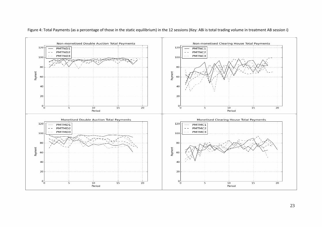
5.3 Payments

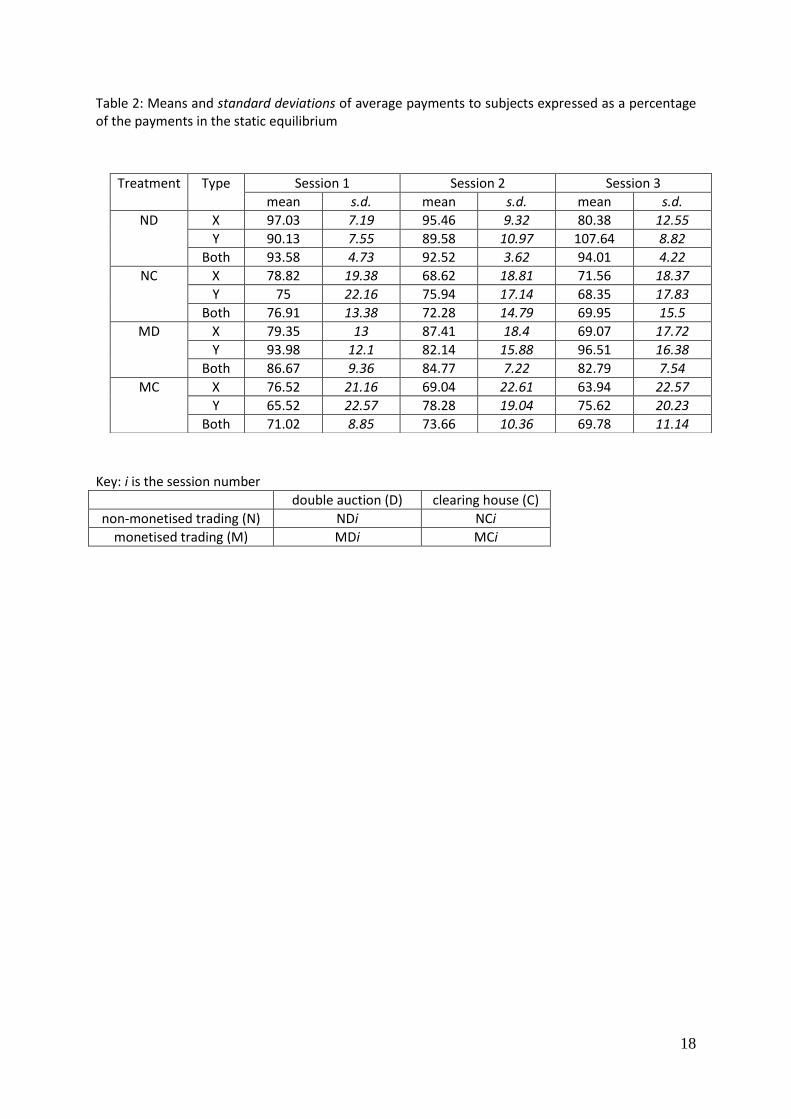
Average payments to subjects per period are shown in Figure 4. Summaries are also presented in

Table 2. In both the Figure and the Table, we present actual payments as a percentage of the

12

payments in the static competitive equilibrium: these latter are €2.00 in sessions 1 and €2.128 in

sessions 2 and 3. It follows from the definition of these variables that the maximum the average can

be in all cases is 100.

In Figure 4 it is clear that in the non-monetised double auction sessions payments to subjects are

around what they should be in the static competitive equilibrium. In the non-monetised clearing

house sessions payments in general were a lot lower than in the non-monetised double auction,

though they were approaching the latter at the end. The same is true in the monetised treatments,

where payments on average to the subjects in the clearing house treatment were lower than in the

double auction. We note that payments were also slightly more erratic in the monetised double

auction as compared with the non-monetised double auction. Going from non-monetised trading to

monetised trading with the double auction sees a decrease in average payments to subjects, while

there was only a small decrease in the average payments to subjects with the clearing house.

However this analysis ignores a trend effect: with the non-monetised clearing house the trend is

upwards throughout the periods of trading, almost reaching 100 by the end, while the monetised

clearing house starts higher but ends up below 100 at the end.

5.4 Efficiency

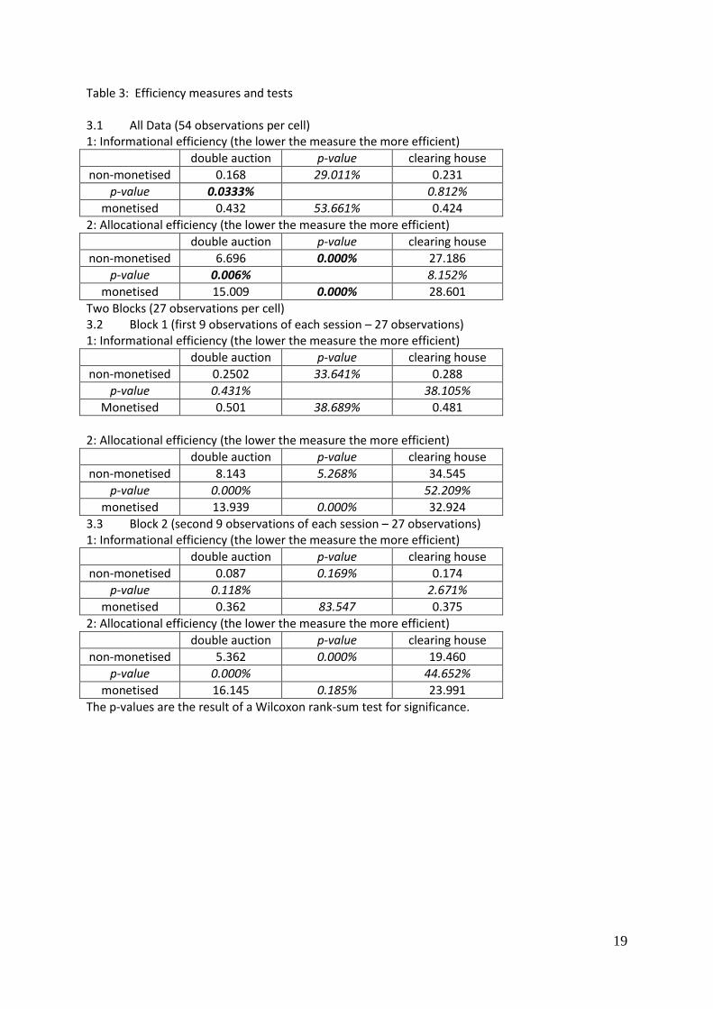
Finally we present some results on efficiency in the four treatments. As we remarked in section 3,

we use two measures – informational efficiency and allocational efficiency. Table 3 shows the

results: 3.1 presents the results on all the data – over the first 189 periods of all six sessions (where

we have 108 observations in each treatment); 3.2 and 3.3 disaggregate the results into the first half

and the second half of each data set (54 observations in each treatment). If we concentrate on all

the data10 – 3.1 – we see that monetised trading lowers the informational and allocational efficiency

8 It should be noted that we chose the various endowments to make these as nearly equal across sessions to

make it fair to the subjects. 9 Different sessions had different lengths and the shortest length was 18.

10 The p-values report the significance levels of the Wilcoxon rank-sum test, between the figures in the

adjacent rows or columns.

13

for both market mechanisms, with the difference being particularly significant for allocational

efficiency for the double auction. Interestingly the clearing house is marginally but not significantly

more informationally efficient than the double auction in the monetised treatment. The breakdown

of the data into the two halves – tables 3.2 and 3.3 – shows that informational efficiency increases

for both trading types as time passes, as one would hope, but allocational efficiency falls for the

double auction.

6. Conclusions

One clear message emerges from these experiments: money hinders convergence to equilibrium. As

a consequence, realised trading volumes in the monetised treatments are lower than they would be

in the static competitive equilibrium, and, of necessity, realised payments/surpluses are lower.

Moreover, switching to a clearing house mechanism does not remove the inefficiencies resulting

from monetised trading. However, we should note that the reduction in payments in the clearing

house is much smaller than the reduction for the double auction, but mainly because the clearing

house starts from a lower base. Indeed, we see markedly lower payments in the clearing house

treatment than in the double auction treatment – a result different from that reported by Friedman

(1993). It is not clear what caused these differences, though it should be noted that in Friedman’s

experiments, trading was always between a good (with a stated value) and real money; in contrast

we have trading between two goods (either directly or indirectly) the value of which depended upon

the combinations of the two goods. Moreover in Friedman’s experiments, which used non-

monetised trading, the price of the trade was always explicit, while in ours the price was implicit in

terms of the ratio of the quantities.

One difficulty facing the subjects in the monetised treatments, and one which is highlighted in the

theoretical literature to which we have referred in section 2, is the question of expectations, crucially

about the value of money. It has a zero value at the (random) end of the experiment, but while the

experiment is continuing, it has a value in that it facilitates the implementation of future trades. All

14

bidding and asking in the monetised treatments had to be done in money terms, and the whole issue

of absolute prices for the two goods is crucial. So far, we have avoided any discussion of absolute

prices – framing all our analyses in terms of relative prices of the two goods – but clearly this is a

factor that would have influenced subjects’ decisions. As the perceived end of the experiment draws

nearer both sides of the market would get increasingly nervous about holding money. However, the

effect of this is not clear, though it may be the case that buyers would be increasingly happy to pay

more, and the sellers would be increasingly happy to ask more. Indeed we notice an increase in the

absolute prices of the two goods as periods pass. But the key issue is on expectations – and these

may be driven by the past behaviour of absolute prices. Thus the results that we have found may

just be consequence of the subjects’ response to the uncertainty about future prices. But this in turn

is linked to the uncertainty about future trades – and this is the whole essence of Clower’s

conjecture.

The bottom line of our experiment is the finding that trading volumes, and payments, in the

monetised treatments are lower than in the non-monetised treatments, and hence lower than they

could/should be in the competitive equilibrium. This finding confirms Clower’s conjecture: that the

necessity of monetised trading may cause lack of trade, and hence, in particular, create involuntary

unemployment. Money does indeed impede convergence.

15

References

Barro, R. J. and Grossman, H. I. (1971), “A General Disequilibrium Model of Income and

Employment”, American Economic Review, 61, 82-93.

Benassy, J.-P. (1975), “Neo-Keynesian Disequilibrium Theory in a Monetary Economy”, Review of

Economic Studies, 42, 203-220.

Cason, T.M. and Friedman, D. (2008), “A Comparison of Market Institutions”, Handbook of

Experimental Economics Results, volume 1, Elsevier.

Clower, R.W. (1967), “A Reconsideration of the Microfoundations of Monetary Theory”, Economic

Inquiry, 6, 1–8.

Crockett, S., Oprea, R. and Plott, C. R. (2011), “Extreme Walrasian Dynamics: The Gale Example in the

Lab”, American Economic Review, 101, 3196-3220.

Friedman, D. (1993), “How Trading Institutions Affect Financial Market Performance: Some

Laboratory Experiments”, Economic Inquiry, 31, 410-435.

Gjerstad, S. (2013), "Price dynamics in an exchange economy", Economic Theory, 52, 461-500.

Goeree, J.K. and Lindsay, L. (2012a), “Designing Package Markets to Eliminate Exposure Risk”,

University of Zurich Working Paper 71.

Goeree, J.K. and Lindsay, L. (2012b), “Stabilizing the Economy: Market Design and General

Equilibrium”, University of Zurich Working Paper.

Greiner, B. (2004), “The Online Recruitment System ORSEE 2.0 - A Guide for the Organization of

Experiments in Economics”. University of Cologne, Working Paper Series in Economics 10.

Hey, J. D. and Di Cagno, D. (1998), “Sequential Markets: An Experimental Investigation of Clower’s

Dual Decision Hypothesis”, Experimental Economics, 1, 63-87.

Kiyotaki N. and Wright R. (1989), “On Money as a Medium of Exchange”. Journal of Political

Economy, 97, 927-954.

Leijonhufvud, A. (1968), On Keynesian Economics and the Economics of Keynes. Oxford: Oxford

University Press.

16

Lucas Jr. R. E. (1980),”Equilibrium in a Pure Monetary Economy”, Economic Inquiry, 18, 203-220.

Ostroy and Starr (1974), “Money and the Decentralization of Exchange”, Econometrica, 42, 1093-

1113.

Shapley, L. and Shubik, M. (1977), “Trade Using One Commodity as a Means of Payment”, Journal of

Political Economy, 85, 937-968.

17

Table 1: Summary statistics on prices and volumes (actual and theoretic)

Treatment Session Endowment of good X of each of the

5 Type X subjects

Endowment of good Y of each of the

5 Type Y subjects

Theoretical relative price of Good Y

Actual average relative price of Good Y

s.d of relative price of Good Y

Actual average trading volume

s.d. of trading volume

ND 1 40 40 1 0.93 0.06 102.84 11.15

2 60 30 2 1.83 0.31 102.64 11.79

3 30 60 0.50 0.67 0.11 99.61 10.76

NC 1` 40 40 1 1.07 0.12 95.04 19.57

2 60 30 2 1.67 0.39 87.42 17.38

3 30 60 0.50 0.66 0.1 79.44 18.51

MD 1 40 40 1 1.33 0.41 65.25 21.25

2 60 30 2 1.95 0.83 76.04 17.82

3 30 60 0.50 0.85 0.3 63.6 19.36

MC 1 40 40 1 1.14 0.35 63 16.7

2 60 30 2 1.68 0.78 56.95 14.76

3 30 60 0.50 0.58 0.4 50.38 14.07

Key: i is the session number




18

Table 2: Means and standard deviations of average payments to subjects expressed as a percentage of the payments in the static equilibrium

Key: i is the session number




Treatment Type Session 1 Session 2 Session 3

mean s.d. mean s.d. mean s.d.

ND X 97.03 7.19 95.46 9.32 80.38 12.55

Y 90.13 7.55 89.58 10.97 107.64 8.82

Both 93.58 4.73 92.52 3.62 94.01 4.22

NC X 78.82 19.38 68.62 18.81 71.56 18.37

Y 75 22.16 75.94 17.14 68.35 17.83

Both 76.91 13.38 72.28 14.79 69.95 15.5

MD X 79.35 13 87.41 18.4 69.07 17.72

Y 93.98 12.1 82.14 15.88 96.51 16.38

Both 86.67 9.36 84.77 7.22 82.79 7.54

MC X 76.52 21.16 69.04 22.61 63.94 22.57

Y 65.52 22.57 78.28 19.04 75.62 20.23

Both 71.02 8.85 73.66 10.36 69.78 11.14

19

Table 3: Efficiency measures and tests 3.1 All Data (54 observations per cell) 1: Informational efficiency (the lower the measure the more efficient)

double auction p-value clearing house

non-monetised 0.168 29.011% 0.231

p-value 0.0333% 0.812%

monetised 0.432 53.661% 0.424

2: Allocational efficiency (the lower the measure the more efficient)


non-monetised 6.696 0.000% 27.186

p-value 0.006% 8.152%

monetised 15.009 0.000% 28.601

Two Blocks (27 observations per cell) 3.2 Block 1 (first 9 observations of each session – 27 observations) 1: Informational efficiency (the lower the measure the more efficient)


non-monetised 0.2502 33.641% 0.288

p-value 0.431% 38.105%

Monetised 0.501 38.689% 0.481



non-monetised 8.143 5.268% 34.545

p-value 0.000% 52.209%

monetised 13.939 0.000% 32.924

3.3 Block 2 (second 9 observations of each session – 27 observations) 1: Informational efficiency (the lower the measure the more efficient)


non-monetised 0.087 0.169% 0.174

p-value 0.118% 2.671%

monetised 0.362 83.547 0.375



non-monetised 5.362 0.000% 19.460

p-value 0.000% 44.652%

monetised 16.145 0.185% 23.991

The p-values are the result of a Wilcoxon rank-sum test for significance.

20

Figure 1: The Relative Prices of Good Y in the 12 sessions. (Key: ABi is relative price in treatment AB session i)

21

Figure 2: Total trading Volumes (as a percentage of those in the static equilibrium) in the 12 sessions (Key: ABi is total trading volume in treatment AB session i)

22

Figure 3: scatters of change in relative price against departure from equilibrium (51 observations in each treatment)

non-monetised trading monetised trading

do

ub

le a

uct

ion

clea

rin

g h

ou

se

23

Figure 4: Total Payments (as a percentage of those in the static equilibrium) in the 12 sessions (Key: ABi is total trading volume in treatment AB session i)

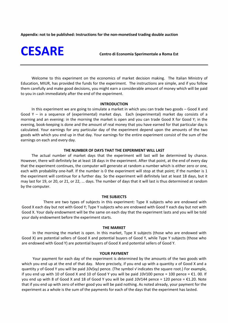
Appendix: not to be published: Instructions for the non-monetised trading double auction

CESARE Centro di Economia Sperimentale a Roma Est

Welcome to this experiment on the economics of market decision making. The Italian Ministry of Education, MIUR, has provided the funds for the experiment. The instructions are simple, and if you follow them carefully and make good decisions, you might earn a considerable amount of money which will be paid to you in cash immediately after the end of the experiment.

INTRODUCTION In this experiment we are going to simulate a market in which you can trade two goods – Good X and Good Y – in a sequence of (experimental) market days. Each (experimental) market day consists of a morning and an evening: in the morning the market is open and you can trade Good X for Good Y; in the evening, book-keeping is done and the amount of real money that you have earned for that particular day is calculated. Your earnings for any particular day of the experiment depend upon the amounts of the two goods with which you end up in that day. Your earnings for the entire experiment consist of the sum of the earnings on each and every day.

THE NUMBER OF DAYS THAT THE EXPERIMENT WILL LAST The actual number of market days that the experiment will last will be determined by chance. However, there will definitely be at least 18 days in the experiment. After that point, at the end of every day that the experiment continues, the computer will generate at random a number which is either zero or one, each with probability one-half. If the number is 0 the experiment will stop at that point; if the number is 1 the experiment will continue for a further day. So the experiment will definitely last at least 18 days, but it may last for 19, or 20, or 21, or 22, ... days. The number of days that it will last is thus determined at random by the computer.

THE SUBJECTS There are two types of subjects in this experiment: Type X subjects who are endowed with

Good X each day but not with Good Y; Type Y subjects who are endowed with Good Y each day but not with Good X. Your daily endowment will be the same on each day that the experiment lasts and you will be told your daily endowment before the experiment starts.

THE MARKET In the morning the market is open. In this market, Type X subjects (those who are endowed with Good X) are potential sellers of Good X and potential buyers of Good Y, while Type Y subjects (those who are endowed with Good Y) are potential buyers of Good X and potential sellers of Good Y.

YOUR PAYMENT Your payment for each day of the experiment is determined by the amounts of the two goods with which you end up at the end of that day. More precisely, if you end up with a quantity x of Good X and a quantity y of Good Y you will be paid 10√(xy) pence. (The symbol √ indicates the square root.) For example, if you end up with 10 of Good X and 10 of Good Y you will be paid 10√100 pence = 100 pence = €1. 00. If you end up with 8 of Good X and 18 of Good Y you will be paid 10√144 pence = 120 pence = €1.20. Note that if you end up with zero of either good you will be paid nothing. As noted already, your payment for the experiment as a whole is the sum of the payments for each of the days that the experiment has lasted.

Please note that you cannot carry stocks of the goods over from one day to the next. THE TRADING MECHANISM

The trading mechanism used in this experiment is what is called the double auction mechanism. Do not worry if you have not encountered this before – it is easy to understand. It is a continuous process, with trading taking place continuously throughout the trading period. At any time during the trading period Type X subjects (those endowed with Good X) can make a bid consisting of a quantity of Good X and a quantity of Good Y – (qX,qY), while Type Y subjects (those endowed with Good Y) can similarly make a bid consisting of a quantity of Good X and a quantity of Good Y – (qX,qY). While these look the same, the interpretation is different. For a Type X subject a bid (qX,qY) means that that subject is willing to offer up to qX units of Good X in exchange for at least qY units of Good Y. For a Type Y subject a bid (qX,qY) means that that subject is willing to offer up to qY units of Good Y in exchange for at least qX units of Good X. We note that only integer values are allowed for the quantities in the bids. Obviously sellers must hold the number of units that they wish to sell. Any such bids will be posted on all screens for all subjects to see. At any time, subjects can accept all or part of any posted bid. Partial acceptance by a Type Y subject of a bid (qX,qY) posted by a Type X subject means that the Type Y subject is willing to supply up to qY units of Good Y accepting in exchange units of Good X at the rate qX/qY. Similarly, partial acceptance by a Type X subject of a bid (qX,qY) posted by a Type Y subject means that the Type X subject is willing to supply up to qX units of Good X accepting in exchange units of Good Y at the rate qY/qX. After acceptance or partial acceptance, the good is traded and accounts adjusted by the computer. This bidding, asking and acceptance process continues throughout the trading period, which lasts for 4 minutes each day.

ACCOUNTING As we have already noted: each subject will be told how many units of the two goods that they have traded; the computer will carry out the appropriate book-keeping. At the end of each day you will be told how many units of the two goods you have ended up with and the earnings implied by these amounts.

PRACTICE SESSIONS In order that you fully understand the experiment, you will be allowed two practice days before the experiment proper starts. The earnings you get in these practice days will not count towards your earnings. TIMEKEEPING

Each market session will last four minutes. A clock on all subjects' screens in the top right hand corner of the screen will display the time left (in minutes and seconds) to the end of that particular session. You will always know how much time is left at any point. OTHER

If you are unsure about any aspect of this experiment please ask one of the experimenters. We hope you find it fruitful.

Appendix: not to be published: Instructions for the non-monetised trading clearing house



INTRODUCTION In this experiment we are going to simulate a market in which you can trade two goods – Good X and Good Y – in a sequence of (experimental) market days. Each (experimental) market day consists of a morning and an evening: in the morning the market is open and you can trade Good X for Good Y; in the afternoon, book-keeping is done and the amount of real money that you have earned for that particular day is calculated. Your earnings for any particular day of the experiment depend upon the amounts of the two goods with which you end up in that day. Your earnings for the entire experiment consist of the sum of the earnings on each and every day.



Good X each day but not with Good Y; Type Y subjects who are endowed with Good Y each day but not with Good X. Your daily endowment will be the same on each day that the experiment lasts. You will be told your Type and your daily endowment before the experiment starts.

THE MARKET In the morning the market is open. In this morning market, Type X subjects (those who are endowed with Good X) are potential sellers of Good X and potential buyers of Good Y, while Type Y subjects (those who are endowed with Good Y) are potential buyers of Good X and potential sellers of Good Y.

YOUR PAYMENT Your payment for each day of the experiment is determined by the amounts of the two goods with which you end up at the end of that day. More precisely, if you end up with a quantity x of Good X and a quantity y of Good Y you will be paid 10√xy pence. (The symbol √ indicates the square root.) For example, if you end up with 10 of Good X and 10 of Good Y you will be paid 10√100 pence = 100 pence = €1. 00. If you end up with 8 of Good X and 18 of Good Y you will be paid 10√144 pence = 120 pence = €1.20. Note that if you end up with zero of either good you will be paid nothing. As noted already, your payment for the experiment as a whole is the sum of the payments for each of the days that the experiment has lasted.

Please note that you cannot carry stocks of the goods over from one day to the next. THE TRADING MECHANISM

The trading mechanism used in this experiment is what is called the clearing house mechanism. Do not worry if you have not encountered this before – it is easy to understand. Type X subjects – those who are endowed with Good X – are asked to make a bid consisting of a quantity of Good X and a quantity of Good Y – (qX ,qY). Similarly Type Y subjects – those who are endowed with Good Y – are asked to make a bid consisting of a quantity of Good X and a quantity of Good Y – (qX ,qY).The Type X’s bid will be interpreted to mean that this subject is willing to trade at most qX units of Good X in exchange for at least qY units of Good Y; if a Type X subject does not want to trade, then no bid should be entered. The Type Y’s bid will be interpreted to mean that this subject is willing to trade at most qY units of Good Y in exchange for at least qX units of Good X; if a Type Y subject does not want to trade, then no bid should be entered. We note that only integer values are allowed for the quantities in the bids. Of course, sellers must actually have the units of the good they are intending to sell. There is a pre-determined time for entering bids and asks, and the computer will display the remaining time. If a subject does not enter a bid, the computer will interpret this as the subject not wanting to trade. When the time has elapsed, the computer will calculate the equilibrium exchange rate between the two goods and the traded quantities in the market. The equilibrium exchange rate will be determined as the exchange rate at which the quantities offered for sale are equal to the quantities demanded for purchase, for both goods. The computer will then inform each subject of the amounts they have bought and the amounts of the other good that they have sold. It is important to note: (1) that a buyer may not be able to buy all the quantity he or she bid for if the implicit exchange rate in the bid is lower than the equilibrium exchange rate or the quantity offered by the sellers is not sufficiently high; (2) that a buyer may pay less than the number of units offered if the equilibrium exchange rate is lower than the exchange rate in the bid; (3) that a seller may not be able to sell all the quantity he or she offered if the exchange rate implicit in the bid is higher than the equilibrium exchange rate or if the quantity demanded by the buyers is not sufficiently high; (4) that a seller may get more than the number of units asked for if the equilibrium exchange rate is higher than the exchange rate implicit in the bid. We note that the equilibrium prices and quantities will be integers.

ACCOUNTING As we have already noted: each subject will be told how many units of the two goods that they have traded. The computer will carry out the appropriate book-keeping. At the end of each day you will be told how many units of the two goods you have ended up with and the earnings implied by these amounts.

PRACTICE SESSIONS

In order that you fully understand the experiment, you will be allowed two practice days before the experiment proper starts. The earnings you get in these practice days will not count towards your earnings. TIMEKEEPING

Each market session will last four minutes. A clock on all subjects' screens in the top right hand corner of the screen will display the time left (in minutes and seconds) to the end of that particular session. You will always know how much time is left at any point. If you do not enter a bid during the time allowed, your bid will be taken to be zero. OTHER


Appendix: not to be published: Instructions for the monetised trading double auction



INTRODUCTION In this experiment we are going to simulate two markets in which you can buy or sell two goods – Good X and Good Y – in a sequence of (experimental) market days. Each (experimental) market day consists of a morning, an afternoon and an evening: in the morning the market for Good X is open and you can buy or sell Good X using (experimental) money; in the afternoon the market for Good Y is open and you may buy or sell Good Y using (experimental) money; in the evening, book-keeping is done and the amount of real money that you have earned for that particular day is calculated. Your earnings for any particular (experimental) day of the experiment depend upon the amounts of the two goods with which you end up in that day. Your earnings for the entire experiment consist of the sum of the earnings on each and every day. The actual experimental money used to facilitate trade during the experiment becomes worthless at the end of it.



Good X each day but not with Good Y; Type Y subjects who are endowed with Good Y each day but not with Good X. Your daily endowment will be the same on each day that the experiment lasts and you will be told your daily endowment before the experiment starts. In addition all subjects are endowed at the beginning of the experiment with some experimental money: this is to facilitate trade only and becomes worthless at the end of the experiment.

THE MARKETS In the morning the market for Good X is open. In this morning market, Type X subjects (those who are endowed with Good X) are potential sellers of the good while Type Y subjects (those who are endowed with Good Y) are potential buyers of the good. In the afternoon the market for Good Y is open. In this afternoon market, Type X subjects (those who are endowed with Good X) are potential buyers of the good while Type Y subjects (those who are endowed with Good Y) are potential sellers of the good. The trading rules are described below.

YOUR PAYMENT

Your payment for each day of the experiment is determined by the amounts of the two goods with which you end up at the end of that day. More precisely, if you end up with a quantity x of Good X and a quantity y of Good Y you will be paid 10√(xy) pence. (The symbol √ indicates the square root.) For example, if you end up with 10 of Good X and 10 of Good Y you will be paid 10√100 pence = 100 pence = €1. 00. If you end up with 8 of Good X and 18 of Good Y you will be paid 10√144 pence = 120 pence = €1.20. Note that if you end up with zero of either good you will be paid nothing. As noted already, your payment for the experiment as a whole is the sum of the payments for each of the days that the experiment has lasted. Please note that you cannot carry stocks of the goods over from one day to the next - experimental money alone can be held from one day to the next. THE TRADING MECHANISM

The trading mechanism used in this experiment is what is called the double auction mechanism. Do not worry if you have not encountered this before – it is easy to understand. It is a continuous process, with trading taking place continuously throughout the trading period. At any time during the trading period potential buyers can make a bid consisting of a price and a quantity – (p,q) – and potential sellers can make an ask consisting also of a price and a quantity – (p,q). A bid (p,q) means that that buyer is willing to pay up to a price p for up to q units of the good. Likewise, an ask (p,q) means that the seller is willing to accept any price down to p for up to q units of the good. We note that only integer values are allowed for the prices and quantities in the bids and asks. Obviously sellers must hold the number of units that they wish to sell and buyers must have the experimental money necessary to pay for the bid (namely pq). Any such bids and asks will be posted on all screens for all traders to see. At any time, buyers can accept all or part of any posted ask and sellers can accept all or part of any posted bid. Partial acceptance of a bid (p,q) by some seller means that the seller will sell up to q units of the good at the price p. Similarly partial acceptance of an ask (p,q) by some buyer means that the buyer will buy up to q units of the good at the price p. After acceptance or partial acceptance, the good is traded and accounts adjusted by the computer. This bidding, asking and acceptance process continues throughout the trading period.

ACCOUNTING As we have already noted: each buyer will be told how many units they have bought and the prices that they paid at the end of each market; each seller will be told how many units they have sold and the prices that they received at the end of each market; The computer will carry out the appropriate book-keeping. At the end of each day you will be told how many units of the two goods you have ended up with and the earnings implied by these amounts, and the amount of experimental money with which you end up the day.

PRACTICE SESSIONS In order that you fully understand the experiment, you will be allowed two practice days before the experiment proper starts. The earnings you get in these practice days will not count towards your earnings. Your endowment of experimental money will be put back to its original amount at the end of the practice days and before the experiment proper starts. TIMEKEEPING

Each market session (morning and afternoon) will last four minutes. A clock on all subjects' screens in the top right hand corner of the screen will display the time left (in minutes and seconds) to the end of that particular session. You will always know how much time is left at any point. OTHER


Appendix: not to be published: Instructions for the monetised trading clearing house



INTRODUCTION In this experiment we are going to simulate two markets in which you can buy or sell two goods – Good X and Good Y – in a sequence of market days. Each market day consists of a morning, an afternoon and an evening: in the morning the market for Good X is open and you can buy or sell Good X using (experimental) money; in the afternoon the market for Good Y is open and you may buy or sell Good Y using (experimental) money; in the evening, book-keeping is done and the amount of real money that you have earned for that particular day is calculated. Your earnings for any particular day of the experiment depend upon the amounts of the two goods with which you end up in that day. Your earnings for the entire experiment consist of the sum of the earnings on each and every day. The actual experimental money used to facilitate trade during the experiment becomes worthless at the end of it.



Good X each day but not with Good Y; Type Y subjects who are endowed with Good Y each day but not with Good X. Your daily endowment will be the same on each day that the experiment lasts. You will be told your Type and your daily endowment before the experiment starts. In addition all subjects are endowed at the beginning of the experiment with some experimental money: this is to facilitate trade only and becomes worthless at the end of the experiment.

THE MARKETS In the morning the market for Good X is open. In this morning market, Type X subjects (those who are endowed with Good X) are potential sellers of the good while Type Y subjects (those who are endowed with Good Y) are potential buyers of the good. In the afternoon the market for Good Y is open. In this afternoon market, Type X subjects (those who are endowed with Good X) are potential buyers of the good while Type Y subjects (those who are endowed with Good Y) are potential sellers of the good. The trading rules are described below.

YOUR PAYMENT

Your payment for each day of the experiment is determined by the amounts of the two goods with which you end up at the end of that day. More precisely, if you end up with a quantity x of Good X and a quantity y of Good Y you will be paid 10√(xy) pence. (The symbol √ indicates the square root.) For example, if you end up with 10 of Good X and 10 of Good Y you will be paid 10√100 pence = 100 pence = €1.00. If you end up with 8 of Good X and 18 of Good Y you will be paid 10√144 pence = 120 pence = €1.20. Note that if you end up with zero of either good you will be paid nothing. As noted already, your payment for the experiment as a whole is the sum of the payments for each of the days that the experiment has lasted.

Please note that you cannot carry stocks of the goods over from one day to the next - experimental money alone can be held from one day to the next. THE TRADING MECHANISM

The trading mechanism used in this experiment is what is called the clearing house mechanism. Do not worry if you have not encountered this before – it is easy to understand. Buyers are asked to make a bid consisting of a price and a quantity – (p,q). Sellers are asked to make an ask consisting also of a price and a quantity – (p,q). The buyer’s bid will be interpreted to mean that the buyer is willing to buy up to the stated quantity at no more than the stated price; if a buyer does not want to buy at any price, then no bid should be entered. The seller’s ask will be interpreted to mean that the seller is willing to sell up to the stated quantity at no less than the stated price; if a seller does not want to sell at any price, no ask should be entered. We note that only integer values are allowed for the prices and quantities in the bids and asks. Of course, buyers must have the (experimental) money with which to finance the purchase; likewise sellers must actually have the units of the good they are intending to sell. There is a pre-determined time for entering bids and asks, and the computer will display the remaining time. If a buyer does not enter a bid, the computer will interpret this as the buyer being unwilling to buy at any price. If a seller does not enter an ask, the computer will interpret this as the seller being unwilling to sell at any price. When the time has elapsed, the computer will calculate the equilibrium price and the traded quantity in the market. The equilibrium price will be determined as the price at which the quantities offered for sale are equal to the quantities demanded for purchase. The computer will then inform each buyer of the amounts they have bought and the price which they paid and will inform each seller of the amounts they have sold and the price which they received. It is important to note: (1) that a buyer may not be able to buy all the quantity he or she bid for if the price in the bid is lower than the equilibrium price or the quantity offered by the sellers is not sufficient; (2) that a buyer may pay less than the price in the bid if the equilibrium price is lower than the price in the bid; (3) that a seller may not be able to sell all the quantity he or she asked for if the price in the ask is higher than the equilibrium price or the quantity demanded by the buyers is not sufficient; (4) that a seller may get more than the price in the ask if the equilibrium price is higher than the price in the ask. We note that the equilibrium prices and quantities will be integers. Occasionally there will be more than one equilibrium price; in such cases the computer will chose one of these at random. ACCOUNTING As we have already noted: each buyer will be told how many units they have bought and the price that they paid at the end of each market; each seller will be told how many units they have sold and the price that they received at the end of each market. The computer will carry out the appropriate book-keeping. At the end of each day you will be told how many units of the two goods you have ended up with and the earnings implied by these amounts, and the amount of experimental money with which you end up the day.

PRACTICE SESSIONS In order that you fully understand the experiment, you will be allowed two practice days before the experiment proper starts. The earnings you get in these practice days will not count towards your earnings.

Your endowment of experimental money will be put back to its original amount at the end of the practice days. TIMEKEEPING

Each market session (morning and afternoon) will last four minutes. A clock on all subjects' screens in the top right hand corner of the screen will display the time left (in minutes and seconds) to the end of that particular session. You will always know how much time is left at any point. If you do not enter a bid or ask during the time allowed, your bid or ask will be taken to be zero OTHER


Documents

Does Money Impede Convergence? - Luiss Guido Carlistatic.luiss.it/RePEc/pdf/cesare/1501.pdf · comparable. _ Lucas (1980), like Barro and Grossman (1971), models an economy with two