Does Parametric fMRI Analysis with SPM

Yield Valid Results? - An Empirical Study of

1484 Rest Datasets

Anders Eklund, Mats Andersson, Camilla Josephson,

Magnus Johannesson and Hans Knutsson

Linköping University Post Print

N.B.: When citing this work, cite the original article.

Original Publication:

Anders Eklund, Mats Andersson, Camilla Josephson, Magnus Johannesson and Hans

Knutsson, Does Parametric fMRI Analysis with SPM Yield Valid Results? - An Empirical

Study of 1484 Rest Datasets, 2012, NeuroImage.

http://dx.doi.org/10.1016/j.neuroimage.2012.03.093

Copyright: Elsevier

http://www.elsevier.com/

Postprint available at: Linköping University Electronic Press

http://urn.kb.se/resolve?urn=urn:nbn:se:liu:diva-76118

Does Parametric fMRI Analysis with SPM Yield Valid Results?-

An Empirical Study of 1484 Rest Datasets

Anders Eklunda,b,∗, Mats Anderssona,b, Camilla Josephsonb,c, Magnus Johannessonc,d, Hans Knutssona,b

aDivision of Medical Informatics, Department of Biomedical Engineering, Linkoping University, Linkoping, SwedenbCenter for Medical Image Science and Visualization (CMIV), Linkoping University, Linkoping, Sweden

cDepartment of Management and Engineering, Linkoping University, Linkoping, SwedendDepartment of Economics, Stockholm School of Economics, Stockholm, Sweden

Abstract

The validity of parametric functional magnetic resonance imaging (fMRI) analysis has only been reported for simulated data.Recent advances in computer science and data sharing make it possible to analyze large amounts of real fMRI data. In this study,1484 rest datasets have been analyzed in SPM8, to estimate true familywise error rates. For a familywise significance threshold of5%, significant activity was found in 1% - 70% of the 1484 rest datasets, depending on repetition time, paradigm and parametersettings. This means that parametric significance thresholds in SPM both can be conservative or very liberal. The main reason forthe high familywise error rates seems to be that the global AR(1) auto correlation correction in SPM fails to model the spectra ofthe residuals, especially for short repetition times. The findings that are reported in this study cannot be generalized to parametricfMRI analysis in general, other software packages may give different results. By using the computational power of the graphicsprocessing unit (GPU), the 1484 rest datasets were also analyzed with a random permutation test. Significant activity was thenfound in 1% - 19% of the datasets. These findings speak to the need for a better model of temporal correlations in fMRI timeseries.

Keywords:Functional magnetic resonance imaging (fMRI), Familywise error rate, Random field theory, Non-parametric statistics, Randompermutation test, Graphics processing unit (GPU)

1. Introduction

It has been debated for a long time if the assumptions that arerequired for standard parametric approaches really are appro-priate for functional magnetic resonance imaging (fMRI) data.It has also been debated how the problem of multiple testingshould be solved. This debate gained new momentum whensignificant brain activity was found in a dead salmon (Bennettet al., 2010). The recent advances in computer science, e.g.graphics processing units (GPUs), make it possible to performconventional fMRI analysis in a few seconds (Eklund et al.,2011a, 2012). This permits using thousands of studies in theevaluation of analysis and inference procedures in fMRI dataanalysis, which was not previously possible. In this study,a large number of rest datasets have been analyzed to showthat temporal correlations in resting state fMRI timeseries mayshow a more complicated structure, than previously assumed inconventional statistical models. Specifically, the autoregressionmodels used by SPM are shown to fail to accommodate a pre-ponderance of low frequencies in resting fMRI timeseries. The

∗Corresponding author at: Division of Medical Informatics, Department ofBiomedical Engineering, Linkoping University, University Hospital, 581 85Linkoping, Sweden, Tel: +46 (0)13 - 28 67 25, Fax: +46 (0)13 - 10 19 02

Email address: anders.eklund@liu.se (Anders Eklund)

result of this is familywise error rates that are higher than theexpected ones, especially for short repetition times.

There have been some studies that show that parametric sig-nificance thresholds from random field theory are conservative,mainly for multi subject fMRI (Poline et al., 1997; Nicholsand Holmes, 2001; Nichols and Hayasaka, 2003; Hayasaka andNichols, 2003a) but also for single subject fMRI (Friston et al.,1994; Hayasaka and Nichols, 2003b). These studies are mainlybased on simulated data, which never can capture all propertiesof real data. The only study that used real data to estimate fami-lywise error rates (Zarahn et al., 1997) merely used 17 datasets,which is inadequate for a good estimate.

The idea of the empirical study is to analyze a large numberof rest (Null) datasets and simply count the number of datasetswith significant activity. If a familywise significance thresholdof 5% is used, activity should be found in 5 out of 100 restdatasets. The empirical study is thus a way to investigate ifthe assumptions about the null distribution hold. An importantnote is that the null hypothesis does not state that there is notany brain activity in rest data (there is always activity in thebrain), but that the rest data do not contain any brain activitythat is correlated with a randomly selected regressor. The maindifficulty of doing such a study is how to get hold of a largenumber of rest datasets.

Preprint submitted to NeuroImage March 29, 2012

2. Data

Resting state fMRI data is commonly collected to study func-tional connectivity (Biswal et al., 1995). As the aim of thisstudy is to investigate Null distributions, resting state fMRI datais what we need. For these reasons, the freely available rest-ing state fMRI datasets in the Neuroimaging Informatics Toolsand Resources Clearinghouse (NITRC) 1000 functional con-nectomes project (Biswal et al., 2010) have been used. The datais fully anonymized and is released under a license that allowsunrestricted non-commercial use, researchers are free to pub-lish any portion of the data set. The enthusiastic researcher canthus repeat the study by using the same data. More informationabout the project can be found at

http://fcon_1000.projects.nitrc.org/ .

A total of 1484 resting state fMRI datasets were downloadedfrom the website, see Table 1 for more information about thedatasets, requiring about 85 GB of storage. For each subjectthere is also a high resolution anatomical volume. The numberof subjects is not 1484, but 1253. For the New Haven data thereare 2 or 4 rest datasets per subject and for the ICBM data thereare 3 rest datasets per subject. We believe that these datasetsare a good representation of different subjects, MR scannersand MR settings.

3. Methods

The 1484 rest datasets were analyzed in SPM81 (updated toversion 4290), by using a Matlab batch script. We chose to usethe SPM software as it, to our knowledge, is the most commonsoftware for fMRI analysis. The findings that are reported inthis study cannot be generalized to parametric fMRI analysis ingeneral, as other fMRI software packages (e.g. FSL2, AFNI3,fmristat4), for example, use other models of the auto correla-tion.

3.1. Preprocessing

Each dataset was first motion corrected and then sevenamounts of smoothing (4, 6, 8, 10, 12, 14, 16 mm FWHM) wereapplied to the motion corrected volumes. Slice timing correc-tion was not applied to the volumes since information about theslice order (i.e. continuous or interleaved) is not available.

The analysis was performed both with and without estimatedmotion parameters as additional regressors in the design ma-trix. The additional regressors will reduce the variance of theresiduals, and can thereby increase the test values. At the sametime, the residual energy at low frequencies can be reduced, asestimated motion parameters often are dominated by low fre-quencies. The spectrum of the residuals can thereby become

1http://www.fil.ion.ucl.ac.uk/spm/2http://www.fmrib.ox.ac.uk/fsl/3http://afni.nimh.nih.gov/afni/4http://www.math.mcgill.ca/keith/fmristat/

more flat (white), resulting in a decrease of the test values. Mo-tion regressors can also reduce spikes and jumps in the data,resulting in a better estimate of the non-sphericity.

The high resolution anatomical volume could have been usedto segment the brain into gray and white matter, but in a numberof cases the registration between the functional dataset and theanatomical dataset failed. The reason for this seems to be thatthe functional and the anatomical data are stored in differentcoordinate systems. Due to this, only the functional datasetswere used in the analysis. As this study is about single subjectfMRI analysis, the datasets were not warped into a standardbrain space.

3.2. Statistical analysis with SPM

The statistical analysis was performed in eight differentways, four block based designs (B1, B2, B3, B4) and four eventrelated designs (E1, E2, E3, E4) were used. The length of ac-tivity and rest periods are given in Table 2. For data that con-forms to Gaussian white noise, the choice of regressors does notmatter. The significance threshold will always be the same, aswhite noise has the same energy for all frequencies and phases.This is, however, not necessarily true for resting state fMRIdata. Two regressors were used for all designs, the stimulusparadigm convolved with the hemodynamic response function(canonical) and its temporal derivative.

Table 2: Length of activity and rest periods, for the block based (B) and theevent related (E) designs, R stands for randomized.

Paradigm Activity periods (s) Rest periods (s)B1 10 10B2 15 15B3 20 20B4 30 30E1 2 6E2 4 8E3 1-4 (R) 3-6 (R)E4 3-6 (R) 4-8 (R)

A t-test value was calculated in each voxel, then a voxel-wise as well as a cluster based threshold, for a familywise errorrate of 5%, was applied. For the cluster based threshold, theactivity map was first thresholded at p = 0.001 (uncorrected).The size of the largest cluster was then compared to the randomfield theory cluster extent threshold (Friston et al., 1994). Thenumber of datasets with significant activity was finally dividedby the number of analyzed datasets, to obtain the familywiseerror rate.

3.3. SPM settings

Except for the small modification of adding time derivatives,the default SPM settings were used in all processing steps (e.g.global AR(1) auto correlation correction, high pass filteringwith a cutoff period of 128 seconds). The variable

defaults.stats.fmri.ufp

2

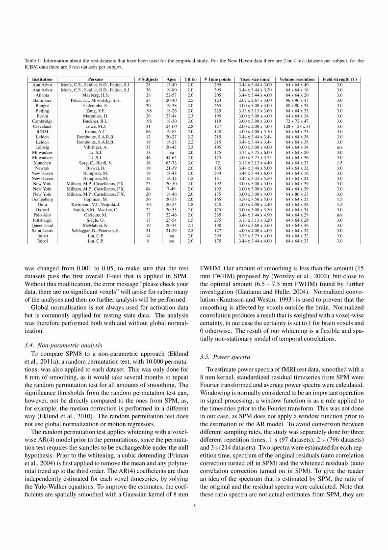
Table 1: Information about the rest datasets that have been used for the empirical study. For the New Haven data there are 2 or 4 rest datasets per subject, for theICBM data there are 3 rest datasets per subject.

Institution Persons # Subjects Ages TR (s) # Time points Voxel size (mm) Volume resolution Field strength (T)Ann Arbor Monk, C.S., Seidler, R.D., Peltier, S.J. 25 13-40 1.0 295 3.44 x 3.44 x 3.00 64 x 64 x 40 3.0Ann Arbor Monk, C.S., Seidler, R.D., Peltier, S.J. 36 19-80 1.0 395 3.44 x 3.44 x 3.20 64 x 64 x 16 3.0

Atlanta Mayberg, H.S. 28 22-57 2.0 205 3.44 x 3.44 x 4.00 64 x 64 x 20 3.0Baltimore Pekar, J.J., Mostofsky, S.H. 23 20-40 2.5 123 2.67 x 2.67 x 3.00 96 x 96 x 47 3.0

Bangor Colcombe, S. 20 19-38 2.0 265 3.00 x 3.00 x 3.00 80 x 80 x 34 3.0Beijing Zang, Y.F. 198 18-26 2.0 225 3.13 x 3.13 x 3.60 64 x 64 x 33 3.0Berlin Margulies, D. 26 23-44 2.3 195 3.00 x 3.00 x 4.00 64 x 64 x 34 3.0

Cambridge Buckner, R.L. 198 18-30 3.0 119 3.00 x 3.00 x 3.00 72 x 72 x 47 3.0Cleveland Lowe, M.J. 31 24-60 2.8 127 2.00 x 2.00 x 4.00 128 x 128 x 31 3.0

ICBM Evans, A.C. 86 19-85 2.0 128 4.00 x 4.00 x 5.50 64 x 64 x 23 3.0Leiden Rombouts, S.A.R.B. 12 20-27 2.2 215 3.44 x 3.44 x 3.44 64 x 64 x 38 3.0Leiden Rombouts, S.A.R.B. 19 18-28 2.2 215 3.44 x 3.44 x 3.44 64 x 64 x 38 3.0Leipzig Villringer, A. 37 20-42 2.3 195 3.00 x 3.00 x 4.00 64 x 64 x 34 n/a

Milwaukee Li, S.J. 18 n/a 2.0 175 3.75 x 3.75 x 6.00 64 x 64 x 20 3.0Milwaukee Li, S.J. 46 44-65 2.0 175 4.00 x 3.75 x 3.75 64 x 64 x 36 3.0Munchen Sorg, C., Riedl, V. 16 63-73 3.0 72 3.13 x 3.13 x 4.40 64 x 64 x 33 1.5Newark Biswal, B. 19 21-39 2.0 135 3.44 x 3.44 x 5.00 64 x 64 x 32 3.0

New Haven Hampson, M. 19 18-48 1.0 249 3.44 x 3.44 x 6.00 64 x 64 x 16 3.0New Haven Hampson, M. 16 18-42 1.5 181 3.44 x 3.44 x 5.50 64 x 64 x 22 3.0New York Milham, M.P., Castellanos, F.X. 25 20-50 2.0 192 3.00 x 3.00 x 3.00 64 x 64 x 39 3.0New York Milham, M.P., Castellanos, F.X. 84 7-49 2.0 192 3.00 x 3.00 x 3.00 64 x 64 x 39 3.0New York Milham, M.P., Castellanos, F.X. 20 18-46 2.0 175 3.00 x 3.00 x 4.00 64 x 80 x 33 3.0

Orangeburg Hoptman, M. 20 20-55 2.0 165 3.50 x 3.50 x 5.00 64 x 64 x 22 1.5Oulu Kiviniemi, V.J., Veijiola, J. 103 20-23 1.8 245 4.00 x 4.00 x 4.40 64 x 64 x 28 1.5

Oxford Smith, S.M., Mackay, C. 22 20-35 2.0 175 3.00 x 3.00 x 3.50 64 x 64 x 34 3.0Palo Alto Greicius, M. 17 22-46 2.0 235 3.44 x 3.44 x 4.90 64 x 64 x 29 n/aPittsburgh Siegle, G. 17 25-54 1.5 275 3.13 x 3.13 x 3.20 64 x 64 x 29 3.0

Queensland McMahon, K. 19 20-34 2.1 190 3.60 x 3.60 x 3.60 64 x 64 x 36 3.0Saint Louis Schlaggar, B., Petersen, S. 31 21-29 2.5 127 4.00 x 4.00 x 4.00 64 x 64 x 32 3.0

Taipei Lin, C.P. 14 n/a 2.0 295 3.75 x 3.75 x 4.00 64 x 64 x 32 3.0Taipei Lin, C.P. 8 n/a 2.0 175 3.44 x 3.44 x 4.00 64 x 64 x 33 3.0

was changed from 0.001 to 0.05, to make sure that the restdatasets pass the first overall F-test that is applied in SPM.Without this modification, the error message ”please check yourdata, there are no significant voxels” will arrise for rather manyof the analyses and then no further analysis will be performed.

Global normalisation is not always used for activation databut is commonly applied for resting state data. The analysiswas therefore performed both with and without global normal-ization.

3.4. Non-parametric analysisTo compare SPM8 to a non-parametric approach (Eklund

et al., 2011a), a random permutation test, with 10 000 permuta-tions, was also applied to each dataset. This was only done for8 mm of smoothing, as it would take several months to repeatthe random permutation test for all amounts of smoothing. Thesignificance thresholds from the random permutation test can,however, not be directly compared to the ones from SPM, as,for example, the motion correction is performed in a differentway (Eklund et al., 2010). The random permutation test doesnot use global normalization or motion regressors.

The random permutation test applies whitening with a voxel-wise AR(4) model prior to the permutations, since the permuta-tion test requires the samples to be exchangeable under the nullhypothesis. Prior to the whitening, a cubic detrending (Frimanet al., 2004) is first applied to remove the mean and any polyno-mial trend up to the third order. The AR(4) coefficients are thenindependently estimated for each voxel timeseries, by solvingthe Yule-Walker equations. To improve the estimates, the coef-ficients are spatially smoothed with a Gaussian kernel of 8 mm

FWHM. Our amount of smoothing is less than the amount (15mm FWHM) proposed by (Worsley et al., 2002), but close tothe optimal amount (6.5 - 7.5 mm FWHM) found by furtherinvestigation (Gautama and Hulle, 2004). Normalized convo-lution (Knutsson and Westin, 1993) is used to prevent that thesmoothing is affected by voxels outside the brain. Normalizedconvolution produces a result that is weighted with a voxel-wisecertainty, in our case the certainty is set to 1 for brain voxels and0 otherwise. The result of our whitening is a flexible and spa-tially non-stationary model of temporal correlations.

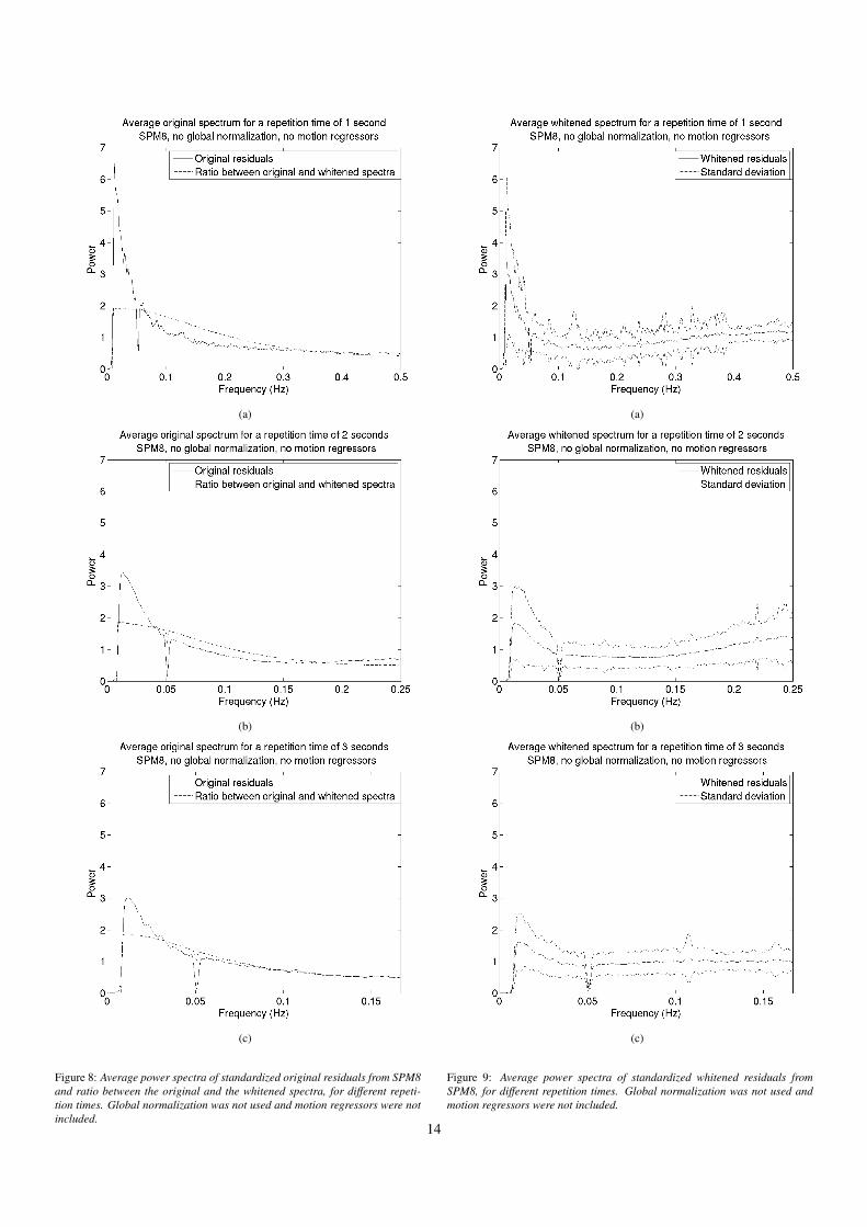
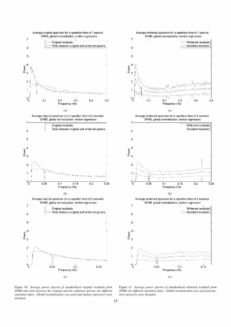
3.5. Power spectra

To estimate power spectra of fMRI rest data, smoothed with a8 mm kernel, standardized residual timeseries from SPM wereFourier transformed and average power spectra were calculated.Windowing is normally considered to be an important operationin signal processing, a window function is as a rule applied tothe timeseries prior to the Fourier transform. This was not donein our case, as SPM does not apply a window function prior tothe estimation of the AR model. To avoid conversion betweendifferent sampling rates, the study was separately done for threedifferent repetition times, 1 s (97 datasets), 2 s (796 datasets)and 3 s (214 datasets). Two spectra were estimated for each rep-etition time, spectrum of the original residuals (auto correlationcorrection turned off in SPM) and the whitened residuals (autocorrelation correction turned on in SPM). To give the readeran idea of the spectrum that is estimated by SPM, the ratio ofthe original and the residual spectra were calculated. Note thatthese ratio spectra are not actual estimates from SPM, they are

3

only used to increase the understanding of SPM’s whitening fordifferent repetition times.

Power spectra were also calculated for the random permuta-tion test, to see the result of the voxel-wise AR(4) whiteningprior to the permutations. All the timeseries were, as standard-ized residuals from SPM8, normalized to have a variance of 1.

3.6. Which parameters affect the familywise error rate?

The GLM framework is based on several assumptions aboutthe residuals. One important assumption is that residuals arewhite (sphericity). This assumption is, for example, related tothe repetition time and if motion regressors are used or not. Thewhitening that is used in SPM assumes that the temporal corre-lations of the residuals are stationary over voxels. This assump-tion could be tested indirectly, by changing the F-test threshold(defaults.stats.fmri.ufp) that determines which voxelsthat are used to estimate the non-sphericity. In our opinion,it is however clear that this assumption is violated. EstimatedAR(1) parameters often yield a spatial pattern that is similar tothe default mode network (Worsley et al., 2002). The whiteningperformance is not likely to be affected by the number of voxelsthat are used to estimate the non-sphericity, as long as the samewhitening is applied to all timeseries.

Random field theory requires the activity map to be smooth,to be a good lattice approximation to random fields. This is re-lated to the amount of smoothing that is applied to the volumes.The smoothing also affects the assumption that the residualsare normally distributed, as smoothing, by the central limit the-orem, will make the data more Gaussian.

A good fMRI software should, for example, be invariant tothe repetition time and the paradigm design and always givevalid results. To determine the analysis parameters that havethe greatest effect on the familywise error rate, we used a binarylogistic regression analysis looking at the effects of smooth-ing, paradigm, repetition time, inference level and the appli-cation of motion regressors and global normalisation (see Ta-ble 3). We repeated a similar analysis for both the SPM8 re-sults and the non-parametric results (omitting the smoothing,motion regressors and global normalisation parameters for thenon-parametric results). The number of analyses (trials) andfalse positives (events) for each level combination were ana-lyzed in Minitab. A significance level of 5% was used to testthe significance of each parameter.

To get independent measurements, it would be necessary touse different datasets for each level combination. The reportedresults are not corrected for dependence between the measure-ments, the significance of each parameter may therefore beoverestimated.

4. Results

Two of the datasets (number 905 and 1310) were removedfrom the study, due to empty brain masks. For some of the82 992 analyses (1482 datasets × 7 amounts of smoothing ×8 paradigms) the error message ”please check your data, thereare no significant voxels” appeared in the SPM software and no

Table 3: Parameters used in the binary logistic regression analysis, and theirlevels.

Parameter LevelsSmoothing Low (4-8 mm), High (10-16 mm)Paradigm Block, Event

Repetition time 1, 3 sInference level Voxel level, Cluster level

Motion regressors No, YesGlobal normalization No, Yes

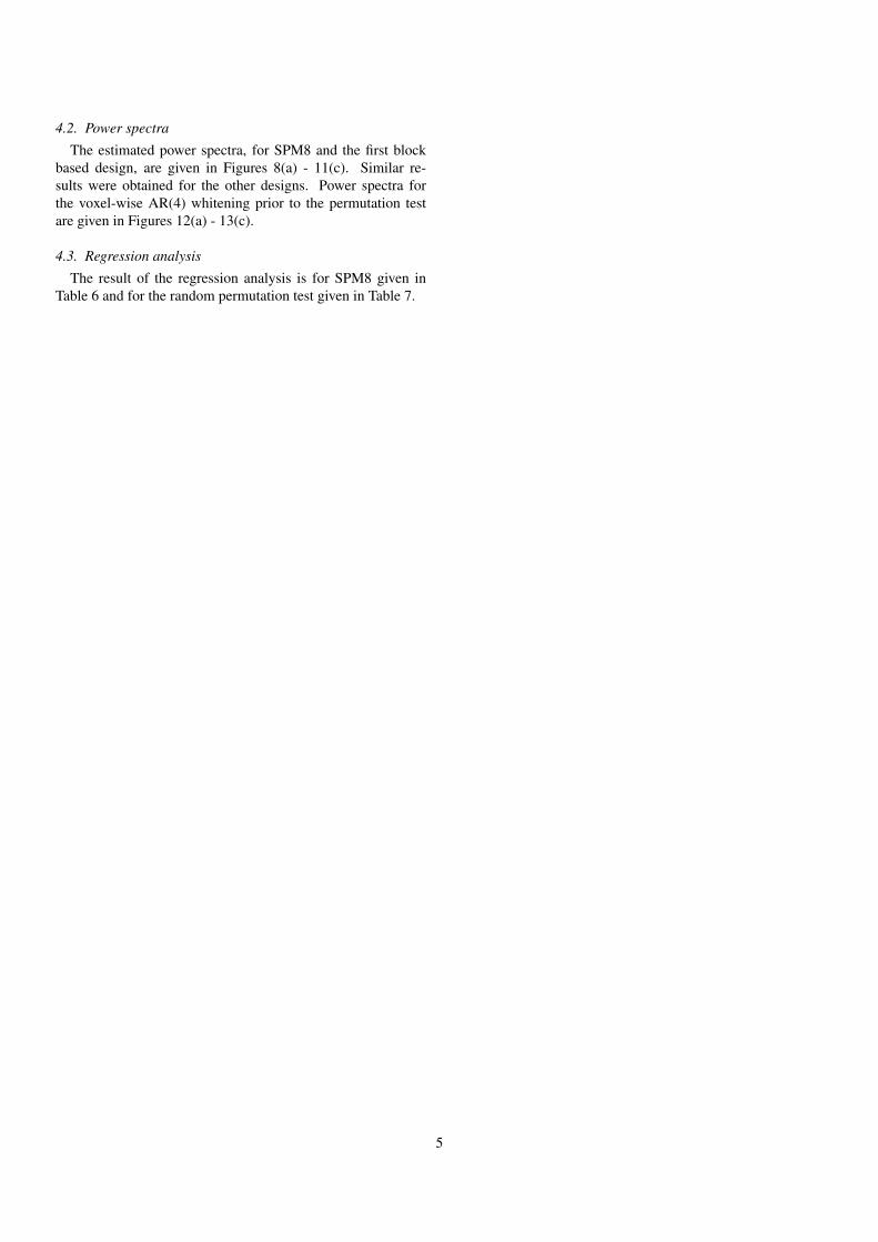
further analysis was performed. The number of occurances fordifferent parameter settings are given in Table 4. The error mes-sage especially appeared for high amounts of smoothing. Forthese cases, the datasets were classified as inactive, i.e. countedas true negatives. The thresholds for these cases are thereforeplotted as zeros.

Table 4: Number of error messages for different parameter settings, out of 82992 analyses per parameter setting, GN = global normalization, MR = motionregressors.

Parameter setting Number of error messagesNo GN, no MR 186

No GN, MR 0GN, no MR 503

GN, MR 20

4.1. Familywise error rates and thresholdsFamilywise error rates for SPM8, without global normaliza-

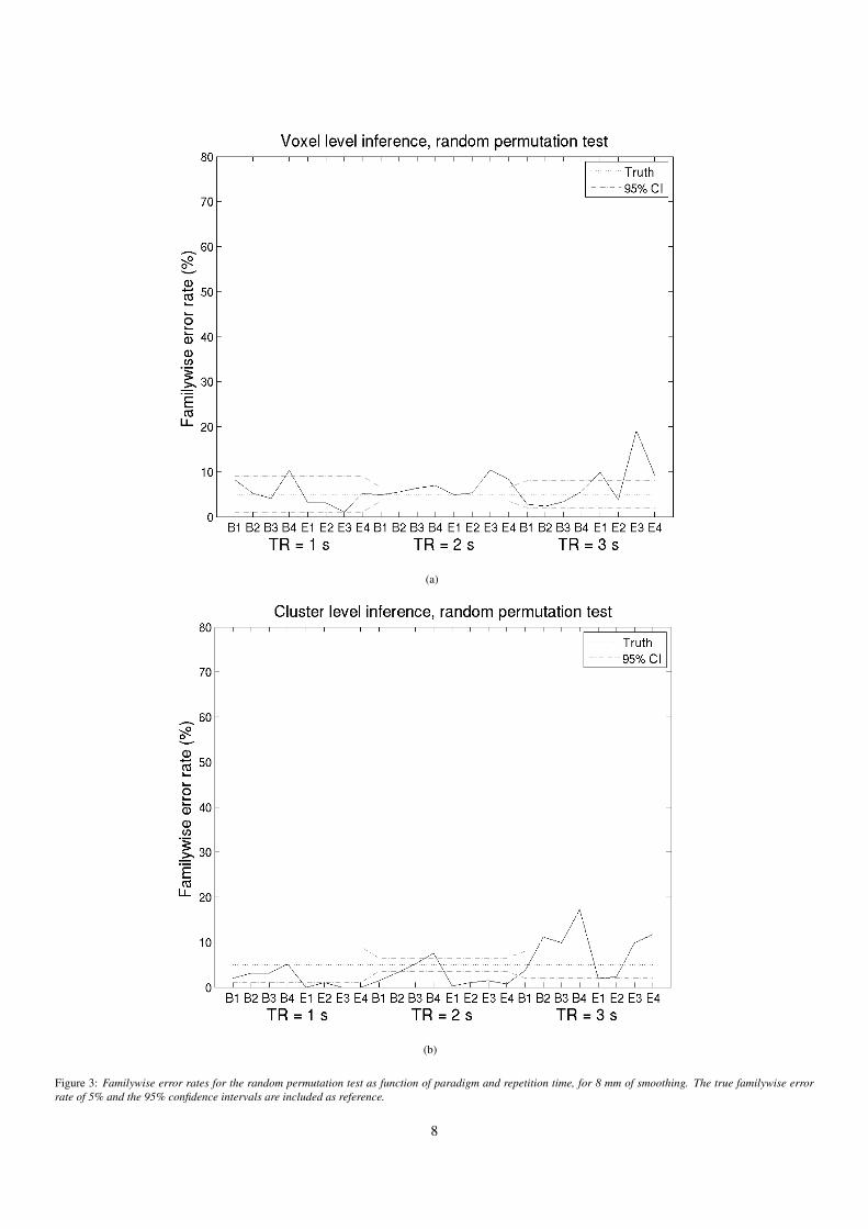
tion and motion regressors, are given in Figures 1(a) - 1(b).Familywise error rates for SPM8, with global normalizationand motion regressors, are given in Figures 2(a) - 2(b). A par-allel coordinate approach (Inselberg, 1985) was used to plot thefamilywise error rate as function of paradigm, smoothing andrepetition time in a 2D plot. Familywise error rates for the ran-dom permutation test are given in Figures 3(a) - 3(b). The es-timated familywise error rates follow a binomial distribution.Approximate 95% confidence intervals for a familywise errorrate of 5%, for different repetition times, are included in thefigures. The confidence intervals are also given in Table 5.

Table 5: Approximate 95% confidence intervals for a familywise error rate of5%, for different repetition times.

Repetition time 95% Confidence interval1 s (97 datasets) 1.0% - 9.0%

2 s (796 datasets) 3.5% - 6.5%3 s (214 datasets) 2.0% - 8.0%

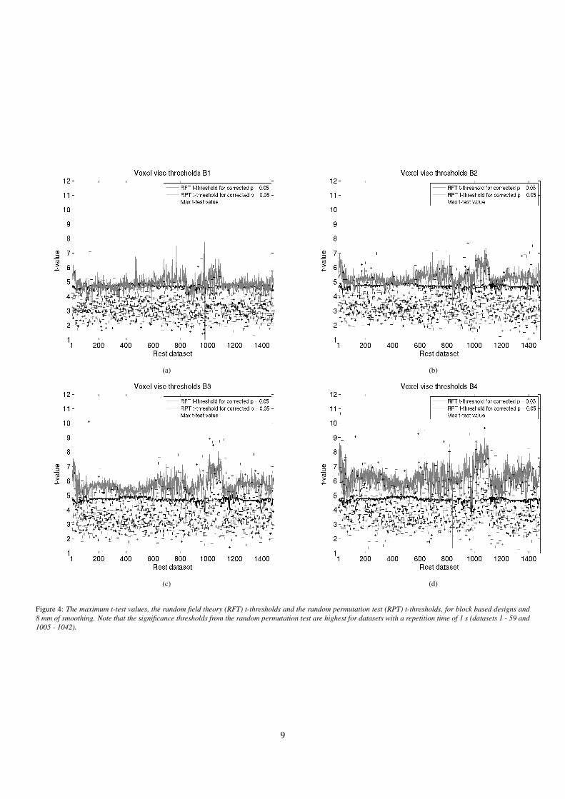
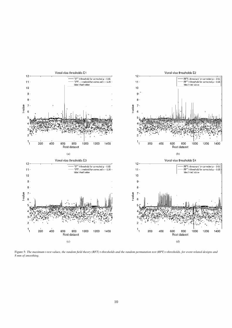
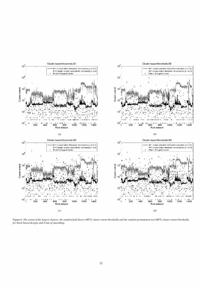
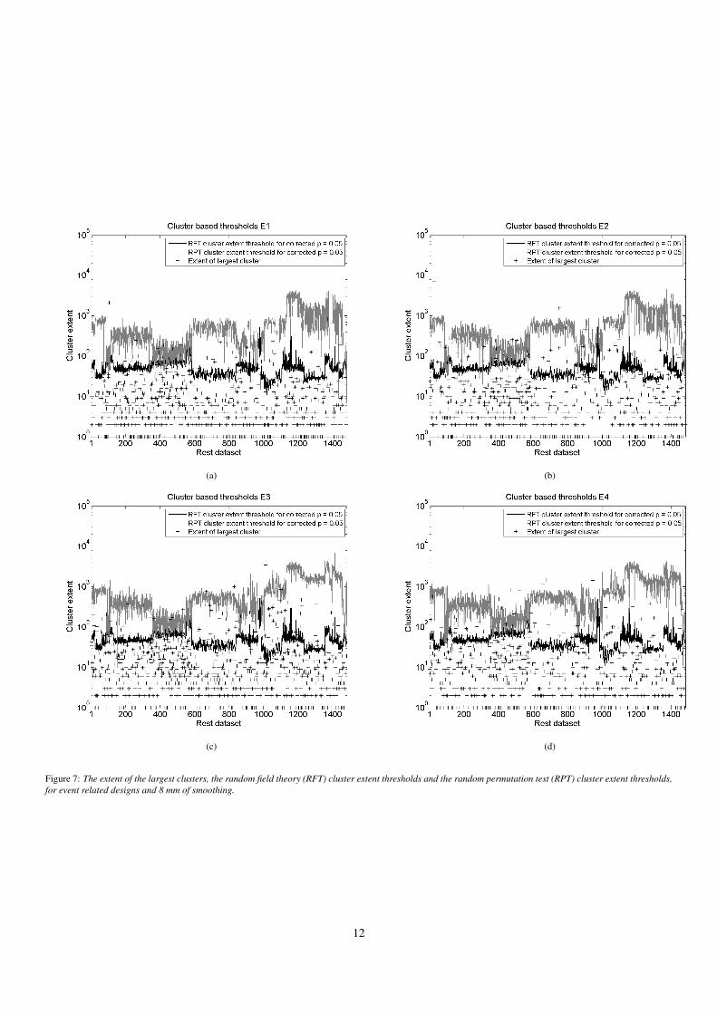
The maximum test values/cluster sizes, the random field the-ory significance thresholds and the random permutation testsignificance thresholds, for 8 mm smoothing, are given in Fig-ures 4(a) - 7(d). The data for these plots were generated withoutglobal normalization and without motion regressors in the de-sign matrix, as the random permutation test does not use thesesettings.

4

4.2. Power spectra

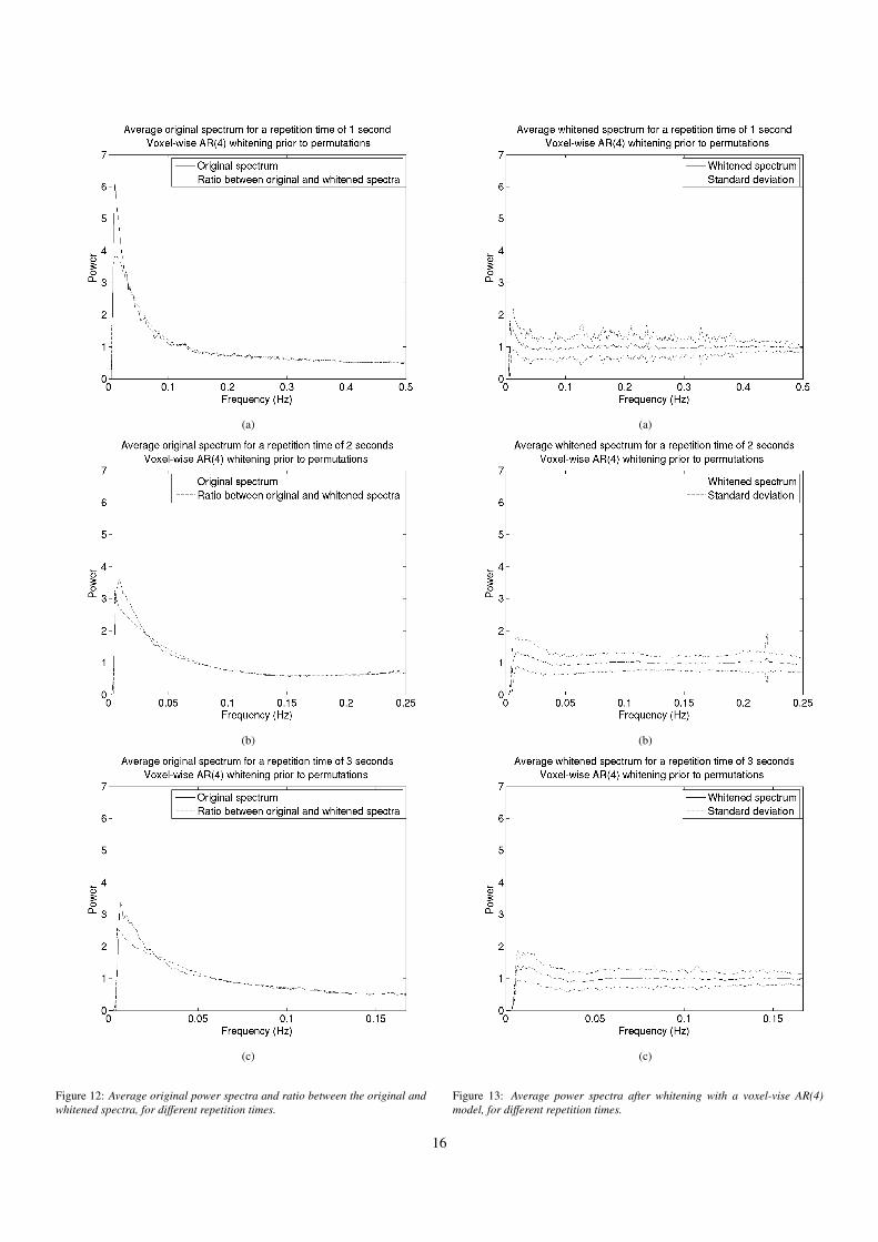
The estimated power spectra, for SPM8 and the first blockbased design, are given in Figures 8(a) - 11(c). Similar re-sults were obtained for the other designs. Power spectra forthe voxel-wise AR(4) whitening prior to the permutation testare given in Figures 12(a) - 13(c).

4.3. Regression analysis

The result of the regression analysis is for SPM8 given inTable 6 and for the random permutation test given in Table 7.

5

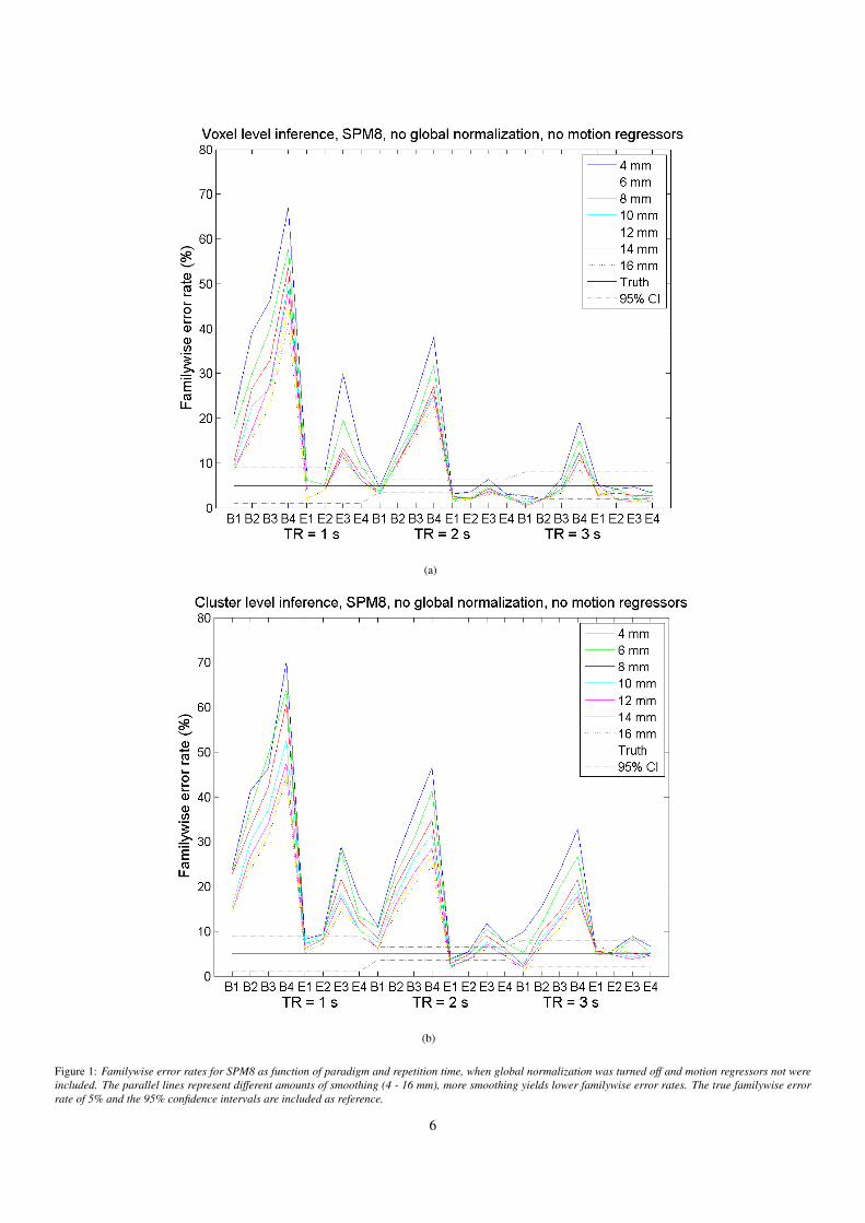
(a)

(b)

Figure 1: Familywise error rates for SPM8 as function of paradigm and repetition time, when global normalization was turned off and motion regressors not wereincluded. The parallel lines represent different amounts of smoothing (4 - 16 mm), more smoothing yields lower familywise error rates. The true familywise errorrate of 5% and the 95% confidence intervals are included as reference.

6

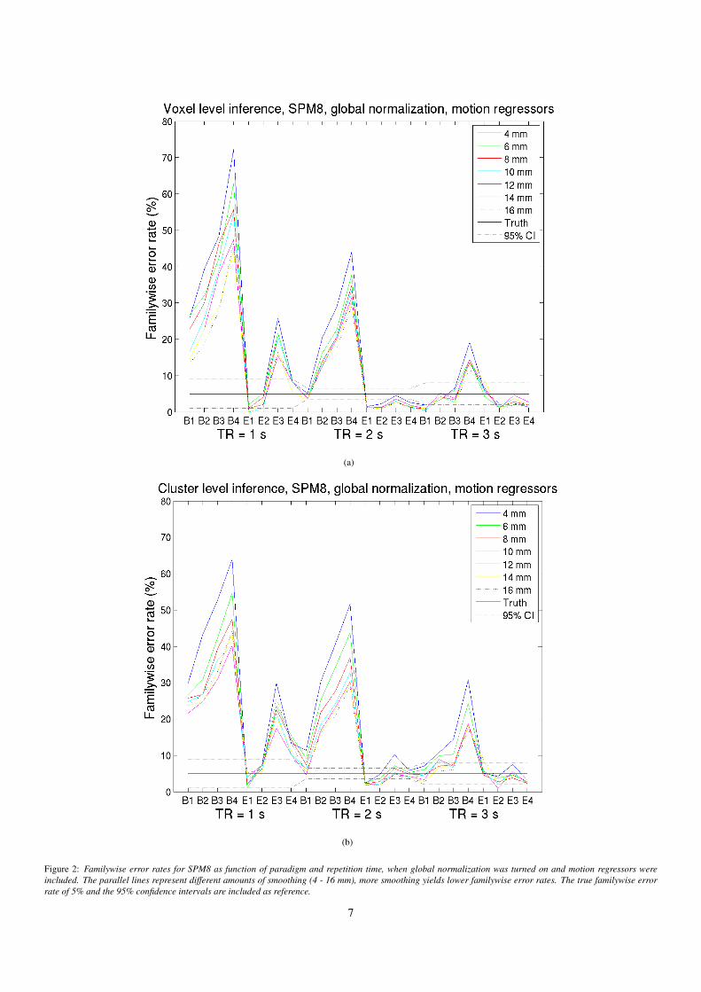
(a)

(b)

Figure 2: Familywise error rates for SPM8 as function of paradigm and repetition time, when global normalization was turned on and motion regressors wereincluded. The parallel lines represent different amounts of smoothing (4 - 16 mm), more smoothing yields lower familywise error rates. The true familywise errorrate of 5% and the 95% confidence intervals are included as reference.

7

(a)

(b)

Figure 3: Familywise error rates for the random permutation test as function of paradigm and repetition time, for 8 mm of smoothing. The true familywise errorrate of 5% and the 95% confidence intervals are included as reference.

8

(a) (b)

(c) (d)

Figure 4: The maximum t-test values, the random field theory (RFT) t-thresholds and the random permutation test (RPT) t-thresholds, for block based designs and8 mm of smoothing. Note that the significance thresholds from the random permutation test are highest for datasets with a repetition time of 1 s (datasets 1 - 59 and1005 - 1042).

9

(a) (b)

(c) (d)

Figure 5: The maximum t-test values, the random field theory (RFT) t-thresholds and the random permutation test (RPT) t-thresholds, for event related designs and8 mm of smoothing.

10

(a) (b)

(c) (d)

Figure 6: The extent of the largest clusters, the random field theory (RFT) cluster extent thresholds and the random permutation test (RPT) cluster extent thresholds,for block based designs and 8 mm of smoothing.

11

(a) (b)

(c) (d)

Figure 7: The extent of the largest clusters, the random field theory (RFT) cluster extent thresholds and the random permutation test (RPT) cluster extent thresholds,for event related designs and 8 mm of smoothing.

12

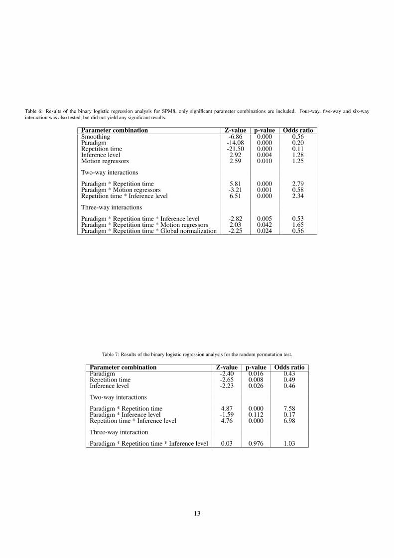
Table 6: Results of the binary logistic regression analysis for SPM8, only significant parameter combinations are included. Four-way, five-way and six-wayinteraction was also tested, but did not yield any significant results.

Parameter combination Z-value p-value Odds ratioSmoothing -6.86 0.000 0.56Paradigm -14.08 0.000 0.20Repetition time -21.50 0.000 0.11Inference level 2.92 0.004 1.28Motion regressors 2.59 0.010 1.25

Two-way interactions

Paradigm * Repetition time 5.81 0.000 2.79Paradigm * Motion regressors -3.21 0.001 0.58Repetition time * Inference level 6.51 0.000 2.34

Three-way interactions

Paradigm * Repetition time * Inference level -2.82 0.005 0.53Paradigm * Repetition time * Motion regressors 2.03 0.042 1.65Paradigm * Repetition time * Global normalization -2.25 0.024 0.56

Table 7: Results of the binary logistic regression analysis for the random permutation test.

Parameter combination Z-value p-value Odds ratioParadigm -2.40 0.016 0.43Repetition time -2.65 0.008 0.49Inference level -2.23 0.026 0.46

Two-way interactions

Paradigm * Repetition time 4.87 0.000 7.58Paradigm * Inference level -1.59 0.112 0.17Repetition time * Inference level 4.76 0.000 6.98

Three-way interaction

Paradigm * Repetition time * Inference level 0.03 0.976 1.03

13

(a)

(b)

(c)

Figure 8: Average power spectra of standardized original residuals from SPM8and ratio between the original and the whitened spectra, for different repeti-tion times. Global normalization was not used and motion regressors were notincluded.

(a)

(b)

(c)

Figure 9: Average power spectra of standardized whitened residuals fromSPM8, for different repetition times. Global normalization was not used andmotion regressors were not included.

14

(a)

(b)

(c)

Figure 10: Average power spectra of standardized original residuals fromSPM8 and ratio between the original and the whitened spectra, for differentrepetition times. Global normalization was used and motion regressors wereincluded.

(a)

(b)

(c)

Figure 11: Average power spectra of standardized whitened residuals fromSPM8, for different repetition times. Global normalization was used and mo-tion regressors were included.

15

(a)

(b)

(c)

Figure 12: Average original power spectra and ratio between the original andwhitened spectra, for different repetition times.

(a)

(b)

(c)

Figure 13: Average power spectra after whitening with a voxel-vise AR(4)model, for different repetition times.

16

5. Discussion

In brief, our analysis of false positive rates reveals some strik-ing and intuitive effects. Overall, a simple AR(1) model fortemporal correlations appears to be adequate for fast designs(E1 and E2) at all three TRs. However, there is a massive in-flation of false positive rates at short TRs that is particularlypronounced for slower (block) designs. At a TR of 1 s, the falsepositive rate can reach up to 70% for block designs. The ef-fect of smoothing is consistent and universal - increasing thesmoothing reduces number of false positives. Furthermore, thiseffect is more pronounced at a shorter TR.

The results are intuitive if we look at the modelling of tem-poral correlations in the frequency domain. The spectra show afailure of the AR(1) model used in SPM to accommodate lowfrequencies, a failure that is exacerbated by short TRs. In otherwords, the AR(1) model fails to account for slow fluctuations inthe residuals that appear to be more prevalent at short TRs. Ourresults are intuitive, because regressors (designs) with lowerfrequency components are clearly more sensitive to the failureof non-sphericity modelling in the low frequency range. In whatfollows we unpack these results and discuss their implicationsfor future modelling work.

5.1. Related studies

We have only found one previous study that estimates fam-ilywise error rates using real data (Zarahn et al., 1997). Therest datasets were analyzed with a block based design withblocks of 40 seconds and the activity maps were thresholdedat p = 0.05 (Bonferroni corrected for multiple testing). Whenindependence was assumed between the time samples, activ-ity was found in 10 out of 17 subjects. For a 1/ f auto corre-lation model, activity was found in 5 subjects. When the se-quences were smoothed with an estimated BOLD impulse re-sponse function, and the 1/ f model of intrinsic auto correlationwas included, activity was found in 1 subject. The same testwithout the auto correlation model resulted in activity in 3 sub-jects.

Another study on rest data from 8 subjects (Smith et al.,2007) used a block based design with blocks of 20 seconds andestimated voxel-wise error rates. When not performing whiten-ing, an uncorrected threshold of p = 0.001 resulted in 862 falsepositives, compared to the expected 58 for 58 000 brain vox-els. When a global AR(1) whitening was applied (as in SPM8),the number of false positives dropped to 109. Similar resultswere found in another study (Purdon and Weisskoff, 1998) andthe problem was found to be more severe for low frequencyblock based designs and short repetition times. A final exampleis a semi-parametric approach to calculate significance thresh-olds (Nandy and Cordes, 2007) which includes a discussionabout the problems with low frequencies in resting state fMRIdata. When rest data were analyzed with a gamma-convolvedboxcar function with blocks of 30 s (B4), activity was foundeven after correcting for multiple testing. The random field the-ory t-threshold was 4.70 and the semi-parametric approach re-sulted in a t-threshold of 6.61.

The results of these studies are consistent with the results ofthe present study, but it is hard to draw strong conclusions asonly a few datasets were used.

5.2. Which parameters affect the familywise error rate?

As can be seen in the plots and in the logistic regressionanalysis, the familywise error rate for SPM8 is significantly af-fected by the amount of smoothing (p < 0.0001, z = -6.86),the paradigm used (p < 0.0001, z = -14.08), the repetition time(p < 0.0001, z = -21.50), the inference level (p = 0.004) andif motion regressors are used or not (p = 0.01). There is alsotwo-way interactions between paradigm and repetition time (p< 0.0001, z = 5.81), between paradigm and motion regressors(p = 0.001) and between repetition time and inference level(p < 0.0001, z = 6.51). Three-way interaction was found be-tween paradigm, repetition time and inference level (p = 0.005),between paradigm, repetition time and motion regressors (p =0.042) and between paradigm, repetition time and global nor-malization (p = 0.024). If multiple testing is considered, andeach test is seen as independent (i.e. Bonferroni adjustment),smoothing, paradigm and repetition time are still significant.The two-way interactions between paradigm and repetition timeand between repetition time and inference level are also stillsignificant.

The random permutation test is also significantly affected bythe repetition time (p = 0.008), the paradigm (p = 0.016) and theinference level (p = 0.026). The z-values for these parametersare, however, lower than for SPM8.

5.3. Non-white noise

The familywise error rates are higher for block based designswith longer periods; this is consistent with the 1/ f model thatis often used for fMRI noise (Zarahn et al., 1997; Smith et al.,1999; Friston et al., 2000). One problem in fMRI is that thesampling rate normally is too low to accurately represent phys-iological noise, such as breathing and heartbeats (Mitra and Pe-saran, 1999; Dagli et al., 1999; Lund et al., 2006). Temporalaliasing is thereby introduced, which invalidates the 1/ f model.Aliasing is probably the reason why the residuals have rela-tively high energy for high frequencies. The familywise errorrates are higher for short repetition times, which previously hasbeen reported for voxel-vise error rates (Purdon and Weisskoff,1998). This is explained by the fact that the auto correlation ofa signal, as function of the sample distance, increases with thesampling frequency (Purdon and Weisskoff, 1998) (but the autocorrelation as function of the time distance is constant). As sub-second repetition times are becoming possible in fMRI (Fein-berg et al., 2010), it is rather alarming that results from SPMare less valid for short repetition times.

The non-white noise (Friman et al., 2005; Lund et al., 2006)can yield p-values that are too low (Purdon and Weisskoff,1998; Lund et al., 2006; Smith et al., 2007). SPM uses high passfiltering as a first remedy. One could remove more of the lowfrequencies, by increasing the cutoff frequency of the high passfilter. This can, however, increase the number of false positiveseven further (Smith et al., 2007). After the high pass filtering,

17

a global AR(1) auto correlation correction is applied (Fristonet al., 2000). The reason why the same AR parameter is usedfor all the brain voxels, is that the effective degrees of freedomvaries between the voxels if an individual whitening is used.As can be seen in Figures 9(a) - 9(c) and 11(a) - 11(c), theglobal AR(1) model used in SPM fails to whiten the residualsfor short repetition times. An explanation for this can be thatthe SPM software was designed when it was common to usevery long repetition times, for which the global AR(1) whiten-ing works rather well. Other software packages for fMRI analy-sis (e.g. FSL, AFNI, fmristat) use more sophisticated modellingof the auto correlation and may potentially yield familywise er-ror rates that are closer to the expected ones.

Our work suggests a need to improve, or extend, the modelsof temporal correlations or stationary dependencies in singlesubject fMRI timeseries. This is a non-trivial problem, sinceone cannot simply estimate the auto correlation function of theresiduals. This follows from the fact that one needs to estimatethe non-sphericity of the underlying random errors, as opposedto the residuals of a general linear model. However, one can-not simply measure the auto correlations in the raw data, be-cause these include dependencies due to signal. This is whyone has to use estimates (for example restricted maximum like-lihood estimators) of the underlying smoothness by making par-ticular assumptions about the form of the unobserved correla-tions among the real errors. Here, the assumption is tempo-ral stationarity, which allows us to represent the non-sphericityin terms of an auto correlation function or spectral density.The problem of non-sphericity is made more acute by the factthat estimating auto correlation functions, from single voxeltimeseries, can lead to inefficient (variable) estimates. Thisis why we smoothed the estimated AR(4) coefficients in thenon-parametric analyses, as for example proposed by (Worsleyet al., 2002). In summary, the advent of very short TR capabili-ties (Feinberg et al., 2010) may call for a re-appraisal of existingassumptions about the form and stationarity of temporal corre-lations in fMRI.

5.4. Non-parametric fMRI analysis

If the exact noise structure was known, a lot of problems infMRI would be solved, but not all of them. Non-parametricfMRI analysis (Siegel, 1957; Dwass, 1957; Holmes et al., 1996;Brammer et al., 1997; Bullmore et al., 2001; Nichols andHolmes, 2001; Nichols and Hayasaka, 2003; Tillikainen et al.,2006; Eklund et al., 2011a) can be required in order to calcu-late significance thresholds and p-values for detection statisticsthat are more advanced than the GLM, for example multi-voxelapproaches, which do not necessarily have a known parametricnull distribution (Friman et al., 2001, 2003; Nandy and Cordes,2003; Mourao-Miranda et al., 2005; Kriegeskorte et al., 2006;Norman et al., 2006; Martino et al., 2008; Bjornsdotter et al.,2011). The beauty of the random permutation test is that it canbe used to calculate significance thresholds and p-values for anytest statistics, for example fMRI analysis by restricted canoni-cal correlation analysis (Das and Sen, 1994; Friman et al., 2003;Eklund et al., 2011a, 2012).

As previously mentioned, the thresholds from the randompermutation test cannot directly be compared to the RFT thresh-olds, as the preprocessing and the statistical analysis is not per-formed exactly as in SPM8. It is, however, clear that the randompermutation test, for voxel level inference, gives higher thresh-olds for the block based designs and slightly lower thresholdsfor the event related designs. Note that the significance thresh-olds from the random permutation test, are highest for datasetswith a repetition time of 1 s (datasets 1 - 59 and 1005 - 1042).The reason why the random permutation test works better forblock based designs, than for event related designs, is probablythat the regressors for the randomized event related designs (E3and E4) have a wider spectra than the other regressors. Thesedesigns are thereby more sensitive to that the whitening prior tothe permutations is correct.

For cluster level inference, the thresholds from the randompermutation test are in general too high. A possible explanationfor this is that cluster based thresholds are more sensitive to aperfect whitening, than voxel-wise thresholds. The whitenedspectra, Figures 13(a) - 13(c), are rather flat, but this does notnecessarily mean that the whitening works for all datasets (andtimeseries). It only means that the whitening works well onaverage. The standard deviation of the whitened spectra fromthe voxel-vise AR(4) whitening is clearly smaller than for thewhitened spectra from SPM.

5.5. Rest vs activity data

It is not straight forward to generalize our findings to stan-dard analyses of activation studies with SPM8. This is becauseresting state data was analyzed, which deliberately promotesslow fluctuations in activity (to estimate functional connectiv-ity or coherence at low temporal frequencies). This means thatthe residuals may be dominated by low frequencies that con-found standard (simple AR) models of serial correlations. Asolution to this problem could be to analyse activity data witha regressor that is orthogonal to the used paradigm. To give anexample, if fMRI activity data has been collected with a blockbased design, analyse the data with an event related design andcount the number of ”false positives”. Data from the OpenfMRIproject,

http://www.openfmri.org,

can be used for this purpose.

5.6. Computational complexity

To analyze an fMRI dataset with 7 amounts of smoothing and8 statistical designs on average takes 10 minutes with SPM8,on an Intel Core i7 3,4 GHz with 16 GB of memory. For 1482datasets this gives a total of 82 992 analyses and a processingtime of about 10 days. The analysis was done with and withoutglobal normalization and motion regressors, yielding a total of331 968 analyses. By instead using the computational powerof the graphics processing unit (GPU) (Gembris et al., 2011; A.R. Ferreira da Silva, 2011, 2010; Eklund et al., 2011a, 2012,2011b) the processing time can be reduced to 5 - 10 secondsper dataset, giving a total processing time of 2 - 4 hours.

18

The main drawback of non-parametric statistical approachesis their computational complexity, which so far has limited theiruse in fMRI. Thresholding techniques for single subject fMRIare more complicated than for multi subject fMRI, as the fMRItime series contain auto correlation (Woolrich et al., 2001). Tobe able to perform a permutation test on single subject fMRIdata, the auto correlations have to be removed prior to the re-sampling (Locascio et al., 1997; Bullmore et al., 2001; Frimanand Westin, 2005), in order to not violate the exchangeabilitycriterion. Single subject fMRI is further complicated by the factthat the spatial smoothing changes the auto correlation struc-ture of the data. This problem is more obvious for CCA basedfMRI analysis, where several filters are applied to the fMRI vol-umes (Friman et al., 2003). The only solution to always havenull data with the same properties, is to perform the spatialsmoothing in each permutation, which significantly increasesthe processing time. This problem was recently solved, by do-ing random permutation tests on the GPU (Eklund et al., 2011a,2012). A random permutation test with 10 000 permutations,for the 8 statistical designs, takes 5-15 minutes per dataset witha multi-GPU implementation, giving a total processing time ofabout 10 days. Note that 10 000 permutations of 85 GB of datais equivalent to analyse 850 TB of data. To perform 11 856 per-mutation tests (1482 datasets × 8 paradigms) with SPM8 wouldtake something like 100 years. We believe that the GPU willbecome an important tool for fMRI analysis.

5.7. Future work

This study has only considered single subject fMRI analysis,but the problems of non-white noise can also affect the resultsof a second-level analysis (Bianciardi et al., 2004). We there-fore intend to repeat the empirical study for multi-subject fMRI.It would also be interesting to repeat the study with other pro-grams for fMRI analysis, such as FSL, AFNI and fmristat, tosee if the more advanced auto correlation modelling results inmore accurate familywise error rates.

To improve the random permutation test, it is possible to usenoise models that are temporally non-stationary (Milosavlje-vic et al., 1995; Long et al., 2005; Luo and Puthusserypady,2007). The important aspect is that there now exists an objec-tive way to compare the correctness of different parametric andnon-parametric approaches.

6. Conclusions

We have presented the results of an empirical study, based on1484 rest datasets, which shows that parametric fMRI analysiswith SPM can give invalid results. The results that are reportedin this paper can, however, not be generalized to parametricfMRI analysis in general, other fMRI software packages maygive different results. The random permutation test works wellin some cases, but indicates that more advanced whitening isnecessary. We challenge other researchers to get better results,and encourage them to repeat the study to verify our findings.To facilitate this, we have put all the datasets, the Matlab scriptsand the results at

http://people.imt.liu.se/andek/rest_fMRI/ .

Acknowledgement

This work was supported by the Linnaeus center CADICS,funded by the Swedish research council, and by the Neuroeco-nomic research group at Linkoping University. NovaMedTechis acknowledged for financial support of the GPU hardware.

The authors would like to thank the Neuroimaging Informat-ics Tools and Resources Clearinghouse (NITRC) and all the in-stitutions that have contributed with data to the 1000 functionalconnectomes project. Without their efforts this empirical studywould not have been possible.

References

A. R. Ferreira da Silva, 2010. cudaBayesreg: Bayesian Computation in CUDA.The R Journal 2/2, 48–55.

A. R. Ferreira da Silva, 2011. A Bayesian multilevel model for fMRI dataanalysis. Computer Methods and Programs in Biomedicine 102, 238–252.

Bennett, C.M., Baird, A.A., Miller, M.B., Wolford, G.L., 2010. Neural corre-lates of interspecies perspective taking in the post-mortem atlantic salmon:An argument for multiple comparisons correction. Journal of Serendipitousand Unexpected Results 1, 1–5.

Bianciardi, M., Cerasa, A., Patria, F., Hagberg, G., 2004. Evaluation of mixedeffects in event-related fMRI studies: Impact of first-level design and filter-ing. NeuroImage 22, 1351–1370.

Biswal, B., Mennes, M., Zuo, X.N., Gohel, S., Kelly, C., Smith, S.M., Beck-mann, C.F., Adelstein, J.S., Buckner, R.L., Colcombe, S., Dogonowski,A.M., Ernst, M., Fair, D., Hampson, M., Hoptman, M.J., Hyde, J.S.,Kiviniemi, V.J., Kotter, R., Li, S.J., Lin, C.P., Lowe, M.J., Mackay, C., Mad-den, D.J., Madsen, K.H., Margulies, D.S., Mayberg, H.S., McMahon, K.,Monk, C.S., Mostofsky, S.H., Nagel, B.J., Pekar, J.J., Peltier, S.J., Petersen,S.E., Riedl, V., Rombouts, S.A., Rypma, B., Schlaggar, B.L., Schmidt, S.,Seidler, R.D., Siegle, G.J., Sorg, C., Teng, G.J., Veijola, J., Villringer, A.,Walter, M., Wang, L., Weng, X.C., Whitfield-Gabrieli, S., Williamson, P.,Windischberger, C., Zang, Y.F., Zhang, H.Y., Castellanos, F.X., Milham,M.P., 2010. Toward discovery science of human brain function. PNAS 107,4734–4739.

Biswal, B., Yetkin, F., Haughton, V., Hyde, J., 1995. Functional connectivityin the motor cortex of resting state human brain using echo-planar MRI.Magnetic Resonance in Medicine 34, 537–541.

Bjornsdotter, M., Rylander, K., Wessberg, J., 2011. A Monte Carlo method forlocally multivariate brain mapping. NeuroImage 56, 508–516.

Brammer, M.J., Bullmore, E.T., Simmons, A., Williams, S.C.R., Grasby, P.M.,Howard, R.J., R.Woodruff, P., Rabe-Hesketh, S., 1997. Generic brain activa-tion mapping in functional magnetic resonance imaging: A nonparametricapproach. Magnetic Resonance Imaging 15, 763–770.

Bullmore, E., Long, C., Suckling, J., Fadili, J., Calvert, G., Zelaya, F., Carpen-ter, T., Brammer, M., 2001. Colored noise and computational inference inneurophysiological fMRI time series analysis: resampling methods in timeand wavelet domains. Human Brain Mapping 12, 61–78.

Dagli, M., Ingeholm, J., Haxby, J., 1999. Localization of cardiac induced signalchange in fMRI. NeuroImage 9, 407–415.

Das, S., Sen, P., 1994. Restricted canonical correlations. Linear Algebra andits Applications 210, 29–47.

Dwass, M., 1957. Modified randomization tests for nonparametric hypotheses.The Annals of Mathematical Statistics 28, 181–187.

Eklund, A., Andersson, M., Knutsson, H., 2010. Phase based volume registra-tion using CUDA, in: IEEE International Conference on Acoustics, Speechand Signal Processing (ICASSP), 2010, pp. 658–661.

Eklund, A., Andersson, M., Knutsson, H., 2011a. Fast random permutationtests enable objective evaluation of methods for single subject fMRI analy-sis. International Journal of Biomedical Imaging, Article ID 627947 .

Eklund, A., Andersson, M., Knutsson, H., 2012. fMRI analysis on theGPU - possibilities and challenges. Computer Methods and Programs inBiomedicine 105, 145–161.

19

Eklund, A., Friman, O., Andersson, M., Knutsson, H., 2011b. A GPU acceler-ated interactive interface for exploratory functional connectivity analysis offMRI data, in: IEEE International Conference on Image Processing (ICIP),pp. 1621–1624.

Feinberg, D.A., Moeller, S., Smith, S.M., Auerbach, E., Ramanna, S., Glasser,M.F., Miller, K.L., Ugurbil, K., Yacoub, E., 2010. Multiplexed echo planarimaging for sub-second whole brain FMRI and fast diffusion imaging. PloSONE 5, e15710.

Friman, O., Borga, M., Lundberg, P., Knutsson, H., 2003. Adaptive analysis offMRI data. NeuroImage 19, 837–845.

Friman, O., Borga, M., Lundberg, P., Knutsson, H., 2004. Detection and de-trending in fMRI data analysis. NeuroImage 22, 645–655.

Friman, O., Carlsson, J., Lundberg, P., Borga, M., Knutsson, H., 2001. Detec-tion of neural activity in functional MRI using canonical correlation analy-sis. Magnetic Resonance in Medicine 45, 323–330.

Friman, O., Morocz, I., Westin, C.F., 2005. Examining the whiteness of fMRInoise, in: Proceedings of the Annual Meeting of the International Society ofMagnetic Resonance in Medicine (ISMRM), p. 699.

Friman, O., Westin, C.F., 2005. Resampling fMRI time series. NeuroImage 25,859–867.

Friston, K., Josephs, O., Zarahn, E., Holmes, A., Rouquette, S., Poline, J.,2000. To smooth or not to smooth - bias and efficiency in fMRI time-seriesanalysis. Neuroimage 12, 196–208.

Friston, K., Worsley, K., Frackowiak, R., Mazziotta, J., Evans, A., 1994. As-sessing the significance of focal activations using their spatial extent. HumanBrain Mapping 1, 210–220.

Gautama, T., Hulle, M.V., 2004. Optimal spatial regularization of autocorrela-tion estimates in fMRI analysis. NeuroImage 23, 1203–1216.

Gembris, D., Neeb, M., Gipp, M., Kugel, A., Manner, R., 2011. Correlationanalysis on GPU systems using NVIDIA’s CUDA. Journal of real-time im-age processing 6, 275–280.

Hayasaka, S., Nichols, T., 2003a. Validating cluster size inference: randomfield and permutation methods. NeuroImage 20, 2343–2356.

Hayasaka, S., Nichols, T., 2003b. Validation of the random field theory-basedcluster size test in single-subject fMRI analyses, in: Proceedings of Interna-tional Society of Magnetic Resonance in Medicine (ISMRM), p. 493.

Holmes, A., Blair, R., Watson, J., Ford, I., 1996. Nonparametric analysis ofstatistic images from functional mapping experiments. Journal of CerebralBlood Flow & Metabolism 16, 7–22.

Inselberg, A., 1985. The plane with parallel coordinates. Visual Computer 1,69–91.

Knutsson, H., Westin, C.F., 1993. Normalized and differential convolution:Methods for interpolation and filtering of incomplete and uncertain data, in:Proceedings of Computer Vision and Pattern Recognition, pp. 515–523.

Kriegeskorte, N., Goebel, R., Bandettini, P., 2006. Information-based func-tional brain mapping. PNAS 103, 3863–3868.

Locascio, J.J., Jennings, P.J., Moore, C.I., Corkin, S., 1997. Time series anal-ysis in the time domain and resampling methods for studies of functionalmagnetic resonance brain imaging. Human Brain Mapping 5, 168–193.

Long, C., Brown, E., Triantafyllou, C., Aharon, I., Wald, L., Solo, V., 2005.Nonstationary noise estimation in functional MRI. NeuroImage 28, 890–903.

Lund, T.E., Madsen, K.H., Sidaros, K., Luo, W.L., Nichols, T.E., 2006. Non-white noise in fMRI: Does modelling have an impact? NeuroImage 29,54–66.

Luo, H., Puthusserypady, S., 2007. fMRI data analysis with nonstationary noisemodels: A bayesian approach. IEEE Transactions on Biomedical Engineer-ing 54, 1621–1630.

Martino, F.D., Valente, G., Staeren, N., Ashburner, J., Goebel, R., Formisano,E., 2008. Combining multivariate voxel selection and support vector ma-chines for mapping and classification of fMRI spatial patterns. NeuroImage43, 44–58.

Milosavljevic, M.M., Veinovic, M.D., Kovacevic, B.D., 1995. Estimation ofnonstationary AR model using the weighted recursive least square algo-rithm, in: IEEE International Conference on Acoustics, Speech and SignalProcessing (ICASSP), 1995, pp. 1432–1435.

Mitra, P.P., Pesaran, B., 1999. Analysis of dynamic brain imaging data. Bio-physical Journal Volume 76, 691–708.

Mourao-Miranda, J., Bokde, A.L., Born, C., Hampel, H., Stetter, M., 2005.Classifying brain states and determining the discriminating activation pat-terns: Support vector machine on functional MRI data. NeuroImage 28,

980–995.Nandy, R., Cordes, D., 2003. A novel nonparametric approach to canonical cor-

relation analysis with applications to low CNR functional MRI data. Mag-netic Resonance in Medicine 49, 1152–1162.

Nandy, R., Cordes, D., 2007. A semi-parametric approach to estimate thefamily-wise error rate in fMRI using resting-state data. NeuroImage 34,1562–1576.

Nichols, T.E., Hayasaka, S., 2003. Controlling the familywise error rate in func-tional neuroimaging: a comparative review. Statistical Methods in MedicalResearch 12, 419–446.

Nichols, T.E., Holmes, A.P., 2001. Nonparametric permutation tests for func-tional neuroimaging: A primer with examples. Human Brain Mapping 15,1–25.

Norman, K.A., Polyn, S.M., Detre, G.J., Haxby, J.V., 2006. Beyond mind-reading: multi-voxel pattern analysis of fMRI data. Trends in CognitiveSciences 10, 424–430.

Poline, J., Worsley, K., Evans, A., Friston, K., 1997. Combining spatial extentand peak intensity to test for activations in functional imaging. NeuroImage5, 83–96.

Purdon, P.L., Weisskoff, R.M., 1998. Effect of temporal autocorrelation dueto physiological noise and stimulus paradigm on voxel-level false-positiverates in fMRI. Human Brain Mapping 6, 239–249.

Siegel, S., 1957. Nonparametric statistics. The American Statistician 11, 13–19.

Smith, A., Lewis, B., Ruttimann, U., Ye, F., Sinnwell, T., Yang, Y., Duyn,J., Frank, J., 1999. Investigation of low frequency drift in fMRI signal.NeuroImage 9, 526–533.

Smith, A.T., Singh, K.D., Balsters, J.H., 2007. A comment on the severity of theeffects of non-white noise in fMRI time-series. NeuroImage 36, 282–288.

Tillikainen, L., Salli, E., Korvenoja, A., Aronen, H., 2006. A cluster masspermutation test with contextual enhancement for fMRI activation detection.Neuroimage 32, 654–664.

Woolrich, M.W., Ripley, B.D., Brady, M., Smith, S.M., 2001. Temporal au-tocorrelation in univariate linear modeling of FMRI data. NeuroImage 14,1370–1386.

Worsley, K., Liao, C., Aston, J., Petre, V., Duncan, G., Morales, F., Evans, A.,2002. A general statistics analysis for fMRI data. NeuroImage 15, 1–15.

Zarahn, E., Aguirre, G., D’Esposito, M., 1997. Empirical analyses of BOLDfMRI statistics I. Spatially unsmoothed data collected under null-hypothesisconditions. NeuroImage 5, 179–197.

20