Does the Diversity of Human Capital Increase GDP?:A Comparison of Education Systems

Katsuya Takii (Osaka U.)and

Ryuichi Tanaka (Titech)

Presentation at GRIPSFebruary 17, 2009

Question 1: What is the relationship between the variance of human capital and GDP?

Japan and Germany

Relatively homogenous labor force (low variance of human capital)

Advantage in production of automobile, consumer electronics, chemical products

Italy and U.S.

high variance of human capital, but many “talented” workers

Advantage in Software industries, financial services, movies

? GDP (h.k.) variance)h.k., averagegiven (For ↑↓⇒↑

Question 2: Which type of education policy is desirable?

Efficiency vs. Equity

• Efficiency: private education, ability tracking => variance (h.k.)

• Equity: public education, no tracking => variance (h.k.)

This paper

Dynamic model of human capital formation (OLG)

(1) Relationship between the variance of h.k. and GDP

(2) Comparison of education systems

The relationship between the variance of h.k. and GDP depends on production technology

Key parameters in production

Complementarity in final good production：

If the production of final good is complement in each individual’s production, the variance of h.k. decreases GDP

ex. Leontief production function

Increasing-returns-to-scale at individual level：

If the production of each individual’s good is IRS, the variance of h.k increases GDP (for given average h.k.)

ex. Superstar (Rosen 1981), Span of control (Lucas 1978)

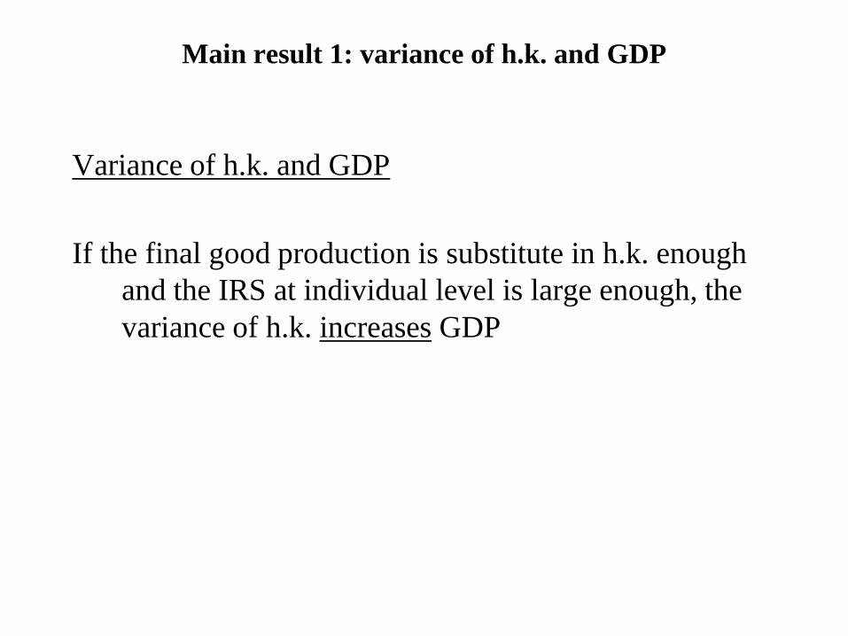
Main result 1: variance of h.k. and GDP

Variance of h.k. and GDP

If the final good production is substitute in h.k. enough and the IRS at individual level is large enough, the variance of h.k. increases GDP

The determinants of the variance of h.k. and educational policy

Determinants of h.k. formation：education investment, individual ability and the quality of peers

Education Finance

• Private education (tuition-financed) => educational investment depends on household income

• Public education (tax-financed) => reduces variance of h.k.

Education program (ability tracking)

• Mixing: decreases the variance of h.k. (equalizing the quality of classmates)• Tracking: increases the variance

Main result 2: comparison of education systems

Program tracking mixing

Finance private A Dpublic C B

1. Under the same education program, public education generates higher GDP than private education (A<C, D<B)

2. Under the same education finance, the effects of tracking on GDP depend on the production parameters (A vs. D, B vs. C)

3. If tracking is available only in private school, private education can generate higher GDP than public education (A vs. B)

Related literatureComparison of Education Finance System

Public education generates higher steady-state GDP than private education if the production function of h.k. is concave and households are credit-constrained (ex. Loury 1981,, Fernandez and Rogerson 1998)

Private generates higher growth rate (Glomm and Ravikumar 1991)

Local vs. Global Complementarities

A stratified economy grows faster than an integrated economy if the local complementarity in education is stronger than the global complementarity in the final good production (ex. Benabou 1996)

Ability Tracking

Ability tracking affects H.K. formation through peer group effect (e.g., Epple and Romano 1998, Epple, Newlon and Romano 2002, Brunello, Giannini and Ariga 2007)

Model：final good production

[ ] )1,0(,)( :function Production/1

∈= ∫ ρρρ dixY i

tt

(GDP)output total:tY tdateat good teintermediath -i :itx

on substituti of elasticity :1)1/(1 >− ρ

[ ] dixpdix it

it

it ∫∫ −

ρρ /1)(max

:producer good final theof problemmax Profit

good teintermediath -i of price :itp

11 )( F.O.C. −−= ρρ itt

it xYp

Intermediate good production

The larger is the h.k., the larger is the use of physical capital (complementarity between h.k. and the size of the project she can manage)

)1,0(,)( :function Production ∈= λλit

it

it khx

i of capitalhuman :ith

good teintermediath -i of production for the used capital physical :itk

1978) (Lucas control ofspan theof degree :λ

itt

it

it krxp −max :problemmax profit si'

)1/(11 )( F.O.C.

λρρρλρ

−

−

= i

ttt

it hY

rk

rateinterest :tr

λρρ

λρρ

λρλρ

λρλρπ −−−

−

−= 11

11

)()1( :profit si' itt

t

it hYr

λ largefor strong is tendency This

GDP and total profit

ρλρ

λρρ

λλλ

λρ−

−−−

=

= ∫

1

1111

)(, GDP dihHHr

Y ittt

tt

GDP increases H.K. of variance the),1

1(11 If

λρ

λρρ

+>⇔>

−

λρρ

λρρλ

λρ

λρλρπ −−−−

−==Π ∫ 11

11)1( Profit Total tt

t

itt HY

rdi

tt Y)1( GDP andprofit talbetween to ipRelationsh λρ−=Π

Human capital formation

11 1

Pub Pri,1 1 1 1

Production function of h.k.

( ) ( ) ( ) , {0,1}, (0,1), 0

( ) , ( ) , : . . . with E( ) 1

i i it t t t

i i i i it t t t t t t t

h U R

U g R e i i d

αφ θ θ

υ υ

ξ θ α φ

ξ ξ ξ ξ

−+ +

+ + + +

= ∈ ∈ > = = =

it

itt 1

,Pri1

Pub1 ,1 :schools privatein only occurs ackingAbility tr 2.

0)(input effective for the negatively-non matters grouppeer ofquality The 1.

sAssumption

+++ ==

≥

ξξξ

υ

[ ]αθθαθυφξ )()()( :form Reduced 111

itt

it

it egh −+

++ =

Preferences3-period-lived OLG:

Continuum of households (normalized to 1) , Each household consists of child, young, and old

– Child receives education – Young earns profit by producing i-th intermediate good, and allocates the

after-tax income to consumption, child’s private education and saving– Old consumes her saving

, ,1 1

11 1

. . (1 ) , (budget constraint)( ) (( ) ( ) ) , (0,1), {0,1} (h.k. production function)

y i i i i o i it t t t t t t t

i i it t t t

s t c e s c r sh e gφ αθυ θ θ α

τ πξ α θ

+ ++ −

+ +

+ + = − == ∈ ∈

iot

it

iyt chc ,

11, lnlnlnmax :problemmax utility si' Young ++ ++ γβ

itt

it

itt

it se πτ

αβθγγπτ

αβθγαβθ )1(

1,)1(

1 F.O.C. −

++=−

++=

Physical capital market

Supply of physical capital at date t+1

Demand for physical capital at date t+1

Market clearing

tti

t dis Π++−

=∫ αβθγτγ

1)1(

∫ ++

+ = 11

1 tt

it Y

rdik λρ

111 )1(1 −

++ Π−++

= tt

tt Yrτγαβθγλρ

Tax choice (majority vote)

Voting

Young votes sincerely for the tax rate that maximizes her own utility for given future interest rate

Equilibrium policy

A policy supported by at lease 50 percent of voters in any pair-wise comparison

Equilibrium Tax rateγαβθαβτ++−

=1

)1(*t

Dynamics of income distribution

Dynamics of household income：

Income distribution),(~ln),2/(~ln),,(~ln 2

11122

12

++++ ∆⇒−∆ ttit

ittt

it mNNmN πσσξπ

BY ttit

it

it

λρθαλρ

λρλρ

λραθυφρ

λραθρ

πξπ −−+

−+−

+−+

++ Π=− 1

)]1([1

)1(1

11

)(

111

)()(

22

22

2

222

1

2

2

2

2

2

2

1

)1()(

)1()(

~2

1)1(

)()1(1)(

2)1(

)1()()1(1)(

tt

ttt

B

mm

∆−

+−+

=∆

+

−

−++−

++

∆

−++

−+−

++=

+

+

λραθρσ

λραθυφρ

σλραθυφρ

ρλραθυφ

θαλλρ

αθρρ

λρλα

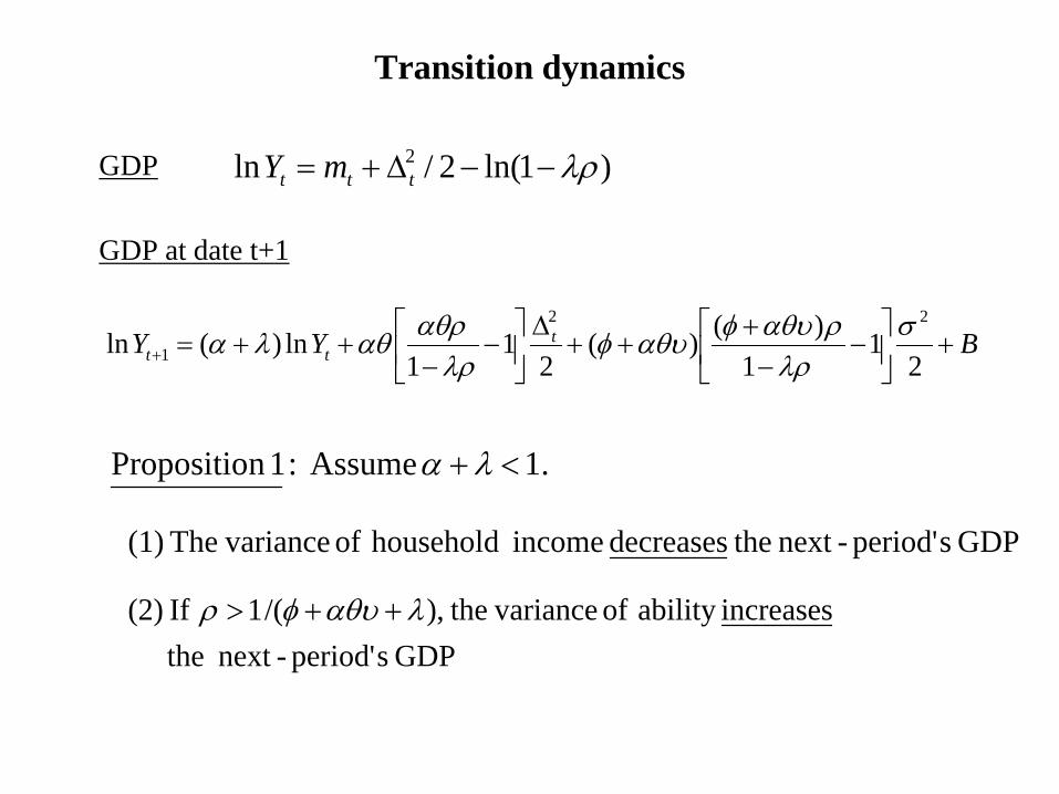
Transition dynamics

GDP

GDP at date t+1

BYY ttt +

−

−+

++∆

−

−++=+ 2

11

)()(2

11

ln)(ln22

1σ

λρραθυφαθυφ

λραθραθλα

)1ln(2/ln 2 λρ−−∆+= ttt mY

.1 Assume :1n Propositio <+ λα

GDP speriod'-next the increasesability of variance the,)/(1 If (2) λαθυφρ ++>

GDP speriod'-next thedecreases income household of varianceThe (1)

Steady-state GDP

Implication: When the elasticity of substitution is larger than the threshold, the association between the steady-state variance of H.K. and steady-state GDP is positive

+

∆+−−

= ∞∞ BDY ~ln

2)(),,,,;(

11ln statesteady in GDP

2

2 αθυφρφυθλαρ

λα

.)1(1 and 1 Suppose :2n Propositio αθυφλλα −+−><+

.1))1(/(1 where)1,(iff0),,,,;( <+−+=∈> λυαθφρρρφυθλαρD

1)2( ))()((),,,,;( 2

−+++++−−−=

λαθυφρλαθυφλαθυφαθαθρφυθλαρD

Public ( ) vs. Private ( ) during transition

IntuitionThe negative effect of the variance of household income on GDP is absent

in public education system

If the variance of ability increases GDP, private education with ability tracking may generate higher GDP than public education

0=θ 1=θ

21

1)2(

21

1lnln

2

?

2Pri

1Pub

1σ

λρραυφαυ

λραρα

−

−+

−∆

−

−−=−

+

++t

tt YY

22Pri1

Pub1

Pri1

Pub1

)(1]1)2([ iff ),2/(1 When (2)

),2/(1 When (1)

3n Propositio

σλαρλαυφρυλαυφρ

λαυφρ

+−−++

>∆>++>

>++≤

++

++

ttt

tt

YY

YY

Public vs. Private in steady state

Implication: When the elasticity of peer group effects is large enough, the private system generates higher steady-state GDP than the public system

−

−+

−∆

−

−−

−−=− ∞

+

∞∞ 21

1)2(

21

111lnln

2

?

Pri,2PriPub σ

λρραυφαυ

λραρα

λα

YY

),,,( iff such that 0),,,( unique a exists there),,,,(each for (2), of case in the Moreover,

)(1]1)2([ iff ),2/(1 When (2)

),2/(1 When (1)

4n Propositio

*PriPub

*

2Pri,2PriPub

PriPub

φρλαυυ

φρλαυφρλα

σλαρλαυφρυλαυφρ

λαυφρ

<>

>

+−−++

>∆>++>

>++≤

∞∞

∞∞∞

∞∞

YY

YY

YY

Ability Tracking in Public School

Public vs. Private

If ability tracking is available both in public and private schools, the public system always generates higher GDP than the private system

Intuition：the negative effect of the variance of household income is absent in the public system

Tracking vs. Mixing in Public School

Whether tracking raises GDP depends on the production parameters

)2/(1 if GDPhigher generates Tracking λαυφρ ++>

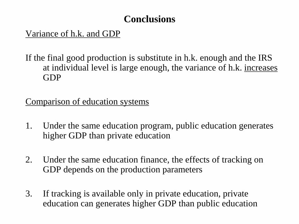
ConclusionsVariance of h.k. and GDP

If the final good production is substitute in h.k. enough and the IRS at individual level is large enough, the variance of h.k. increasesGDP

Comparison of education systems

1. Under the same education program, public education generates higher GDP than private education

2. Under the same education finance, the effects of tracking on GDP depends on the production parameters

3. If tracking is available only in private education, private education can generates higher GDP than public education

DiscussionsDependence of child’s ability on parent’s ability

All results are qualitatively unchanged

Steady-state welfare comparisonNot only GDP but also income inequality matter for the comparisonIf tracking is given, public is better than private in terms of welfare

On the relevance of trade off between income inequality and diversity The elasticity of substitution of intermediate goods: ρ=5/6

(20 per cent markup as in Christiano, Eichenbaum and Evans, 2005)Labor share: 1−λρ = 2/3 => λ = 0.4 => ρ>1/(1+ λ)α <1−λ =0.6φ =1 (as in Benabou 1996)If αθν <φ=1, then Yt+1 is strictly increasing in σ2 .