Embed Size (px)
Citation preview

Does the Fairness of the Distribution of Wealth
Affect Individual Labour Supply?
Maureen Paul
University of Warwick
Coventry
CV4 7AL
April 1, 2004
Abstract
Expanding on the theory put forward by Akerlof (1980) on the role of social custom in
economic behaviour, this paper develops a simple theoretical model that explains how
an individual’s labour supply decision may be affected by the fairness of the wealth
distribution. The accompanying empirical analysis supports the theoretical conclusion
that individual labour supply and the fairness of the wealth distribution may be pos-
itively related. Specifically, using panel data, the within-group estimates reveal that
for the average male employee, labour supply tends to fall as fairness perceptions of
the wealth distribution becomes more unfavourable. Where productivity is concerned,
this study may help understand the differences between egalitarian and less egalitarian
societies.
Key words : Social norms; Labour supply; Fairness; Wealth distribution
JEL Classification: C23; C25; D11; D12; D31; D63; J22
1 Introduction
Wealth inequality and its effects are a matter of huge concern for the global body
politic. In fact, it has remained a preoccupation of both economists and politicians.
Notwithstanding, wealth inequality has continued to increase within countries (see
Korzeniewicz and Moran (1997), Foster and Pearson (2002) and Milanovic (2002)
inter alia) and between countries (see Goodman (2001) and Sala-i-Martin (2002) inter
alia). In response, many individuals engage in protests1. Some of these protests are
vocal and often take the form of visible demonstrations. Others are less visible as
in the case of individuals engaging in non-paid voluntary activities aimed at helping
the disadvantaged or refusing to support governments or companies thought to be
purveyors of inequality.
The prevalence of voluntary activities in the UK is revealed from surveys commis-
sioned by the Institute for Volunteering Research (IVR) in 1991 and 19972. It was found
that in both years, approximately 50 percent of the UK adult population engaged in
formally organised voluntary activities (which is defined as work arranged through an
organisation) whilst well over 70 percent was involved in informal voluntary activities
(that is, work done on an individual basis). What is more substantive and salient is
the finding that the number of hours that the existing volunteers spent per week on
voluntary work increased by 50 percent – up from an average of 2.70 hours in 1991 to
4.05 hours in 19973. Much of this increase was due to a growth in activities aimed at
1Some might argue that an unequal wealth distribution has been the catalyst for much of the
recent conflict within and across nations and the ensuing protests.
2The first survey was carried out in 1981. The reports are available via the web site at
www.ivr.org.uk.
3The total number of hours volunteered increased from 62 million in 1991 to 88 million in 1997.
1
helping the disadvantaged.
The increase in the number of hours spent on voluntary work coincides with an
increase in wealth inequality in the UK. From 1991 to 1997, the percentage of wealth
owned by the top 10 percent of the wealthiest individuals, increased from 47 percent
to 54 percent4. Evidence from the IVR surveys suggest that these two may indeed
be correlated. It was discovered that a large proportion of individuals who undertake
voluntary work do so for purely altruistic reasons and many believe that there would
be no need for volunteers if the government met all its obligations such as, one would
imagine, achieving a more equitable wealth distribution.
Individuals’ volition to take action that are clearly costly to them (for example, lost
labour income or more broadly lost consumption) can be rationalised by the existence
of social norms. Social norms are a pervasive part of economic life and thus, can
exercise decisive influence over individuals’ decision process. Their violation by self or
by others may lead to a loss of “psychic income” and the underprovision of a public
good.
The survival of norms depends on the willingness of individuals to act in ways that
enforces and preserves them. Ergo, it can be argued, if there is a general concern
for fairness and the norm of fairness is violated, as in the case of an unfair wealth
distribution, individuals will seek to reduce the consequent loss of psychic income and
maintain this public good by devoting time and effort towards activities aimed at
restoring a fair state. In this way, wealth inequality may be negatively correlated with
the time dedicated to labour market work. At this juncture, it is interesting to note
that it is employed individuals who are most likely to do voluntary work5.
4Data are obtained from the Office of National Statistics, which are available at
http://www.statistics.gov.uk.
5This is based on the findings of the 1991 and 1997 surveys on voluntary work commissioned by
2

However, it is not possible to rule out a priori a positive relationship between
wealth inequality and hours of work. For instance, it is possible that greater inequality
in society may serve to undermine or erode social norms and encourage more individu-
alistic and competitive behaviour. As a result individuals would be motivated to work
harder6.
Yet, though there exists broad awareness of the impact of wealth inequality at the
macro level, particularly in the case of productivity7, little is known of its influence
on the micro level choices of individuals, which one might expect to lie behind the
macro outcomes. Certainly, it does not appear that there are any studies which have
sought to discover whether individual labour supply responds in a meaningful way to
changes in the equality or fairness of the wealth distribution. On the other hand, whilst
there are microeconomic analyses of the impact of fairness violations by one agent on
the effort choice of the individual who is directly affected (see Adams and Rosenbaum
(1962) and Fehr et al (1993) inter alia), the importance of individuals concern for
distributional fairness, that is whether they are directly affected by unfairness or not,
is often overlooked.
This paper thus seeks to investigate whether an unfair wealth distribution has a
deleterious impact on labour supply. It finds that, for male individuals, labour supply
decisions are not based solely on pecuniary concerns. Indeed, concern for a fair wealth
distribution matters.
the Institute for Volunteering Research.
6That is, individuals might seek to keep up with the Joneses and ahead of the Smiths by working
harder in order to increase income.
7See for example the influential works of Galor and Zeira (1993) and Persson and Tabellini (1994)
inter alia.
3
The rest of the paper is organised as follows. In Section 2 a brief overview of
the related literature is provided. Section 3 develops a simple theoretical model to
explain how an unfair wealth distribution may impact on the labour supply decision
of the individual. The theoretical predictions of the model then form the basis of the
empirical analysis which is presented in Section 4. Section 5 concludes.
2 A brief overview of related studies
The labour supply of individuals represents perhaps the most productive resource of
an economy. Hence, understanding what determines individual labour supply is of
paramount importance and indeed much effort has been dedicated to the study of the
determinants of labour supply. A systematic analysis of some of the major studies
can be found in Ashenfelter and Layard (1986). Nonetheless, there remains a paucity
of studies that explore the importance of factors that reflect individuals’ values and
opinions.
As with other aspects of life, an individual’s labour market behaviour is shaped in
part by social norms. For instance, in some societies male members are expected to be
in full-time employment and to be the main bread winners whereas the same level of
attachment to the labour market is not expected from female members. Instead, women
are expected to devote more time to the care of the home and community. Therefore,
social norms that prescribe the societal roles of men and women may influence the
amount of time the individual commits to labour market work (see for example Stutzer
and Lalive (2001), Feldman(2002), and Cornwell et al (2000)) and even how much effort
he expends (see Levine (1992)). Whilst these studies provide implicit reasons why social
norms may affect labour market behaviour they do not provide a formal framework
within which the effect of social norms on marginal choices might be established.
The theoretical model of Akerlof (1980) offers a more formal conceptualisation of
4

this implicit proposition that social norms affect marginal choices. Extending the
standard utility function, Akerlof (1980) demonstrates how social customs may enter
non-additively in the utility function and in so doing affect labour market behaviour.
His approach rests on the premise that when there is a common willingness to punish
those who deviate from accepted behaviour, the desire to pursue pecuniary gains is
tempered by the costs of deviation. Building further on this idea while narrowing the
focus, de Neubourg and Vendrik (1994) illustrate how some social norms can influence
the labour supply decision of the individual and how these norms may account for the
differences between male and female labour supply behaviour. However, these studies
only concentrate on what may be described as local violations of norms in that they
restrict consideration to how an individual’s behaviour is affected if he violates a social
norm. Neither study has explicitly considered how an individual’s economic behaviour
is influenced by the violation of social norms at the global level. Likewise, it appears
that most studies focusing on specific norms prefer to concentrate on local violations,
be it by the individual in concern or by some other agent.
A particular norm, which has attracted considerable attention of late, is the norm of
fairness. Where work is concerned, fairness considerations appear to play a role in effort
choice determination. This is persuasively corroborated by theoretical arguments such
as that of Akerlof (1982) and Akerlof and Yellen (1990) and supported by experimental
evidence both in the social psychology and economics literature. Studies such as those
by Adams and Rosenbaum (1962), Andrews (1967), and Fehr et al (1993) inter alia
conclude that effort is positively related to the (perceived) fairness of the pay received.
They typically found that fairness concerns affect individuals’ effective labour supply.
Specifically, it was found that when individuals are treated unfairly with regard to pay,
they respond by reducing their effort level and when they believe they are generously
remunerated, they appear to increase their effort levels above the minimum required.
In other words, individuals appear to abide by the ethos ‘a fair day’s work for a fair
5
day’s pay’.
Of course, it is not only the fear of retribution for violating the norm of fairness
nor when unfairness is directed towards them that individuals care about fairness.
Individuals have a preference for fairness which is seen, for example, through their
wish to support redistributive measures (see Carlsson et al (2001), Fong (2001) and
Corneo and Gruner (2002) inter alia)8 and their desire to punish those who are reputed
to behave unfairly regardless of the object of the unfairness (see for example, Thaler
(1985) and Kahneman et al (1986a, 1986b)). Indeed, when the norm of fairness is
violated, individuals suffer a loss of psychic income. That is, unfairness is a bad
that leads to ‘cognitive dissonance’. This means that preference for fairness would be
in conflict with the experience of unfairness. Moreover, individuals feel displeasure
because of associated emotions such as guilt, pity and anger. As a result, they may
take remedial action, which includes changing their beliefs to achieve consonance, in
an attempt to reduce this loss. Coupled with the proposition that social norms affect
marginal choices, this implies that concerns for distributional fairness can instruct
much of the individual’s decision-making not least his labour supply choice.
On the whole, it can be said that, through theoretical arguments and experimental
evidence, the literature has succeeded in showing that economic behaviour may be
informed by social norms and, of importance here, that an individual’s effective labour
supply may respond to unfairness particularly when the individual is directly affected
by the unfair outcome. Hitherto however, it does not appear that there are any studies
that endeavour to discover whether and how global concerns for fairness might affect
microeconomic choices. This present study addresses this gap in the literature by
8This is lucidly conveyed by the statement ”People might not support the redistributive program
which maximizes their private benefit, but the one which conforms with their vision of what constitutes
a good policy for society as a whole” (Corneo and Gruner (2002)).
6
providing an analysis of the possible effects that concerns for distributional fairness
may have on labour market behaviour. It also complements existing experimental
studies by providing a non-experimental analysis of the role of fairness perceptions in
shaping individual labour supply behaviour.
3 How might the fairness of the wealth distribution
affect labour supply?
3.1 A basic framework
The canonical model of labour supply often presented in textbooks postulates that an
individual’s labour supply decision rests upon the maximisation of the following utility
function:
U(X, L) (1)
subject to:
PX ≤ Y = Yn + wH (income budget constraint) (2)
T = H + L (time budget constraint) (3)
where T is the total time available, H is the number of hours out of T spent working and
L is the total time out of T spent on leisure, which is taken here to represent time spent
engaged in activities other than labour market activities. Total disposable income, Y ,
consists of non-labour income, Yn, and labour income, wH, with w being the hourly
wage rate. All the goods and services consumed by the individual is represented by X
and P is the price of this composite commodity.
7
The role of non-pecuniary preferences, such as fairness considerations, in shaping
individual’s labour supply choice is largely ignored in this model. Instead emphasis is
essentially placed on pecuniary preferences. This is however, an inadequate represen-
tation of the reality. As is now widely accepted by economists, non-pecuniary concerns
can and do have decisive bearing on microeconomic outcomes9. Of particular relevance
here is the model of de Neubourg and Vendrik (1994). Following the model of Akerlof
(1980), they argue that social norms enter non-additively in the utility function and
can therefore shape labour market behaviour.
Maintaining the assumption that social norms affect marginal choices, the canonical
model is reformulated in this study to explicitly take into account the norm of fairness
a propos the wealth distribution. For the sake of simplicity, it is assumed that the
societal norm of fairness is both well-established and accepted by all, though agents
care to different extents about the fairness of the wealth distribution. Hence, individ-
uals are believed to be both altruistic in that they care that others are treated fairly,
feeling discomfort when they are not and self-centred, that is to say they care that
they as individuals are treated fairly, feeling resentful when they are not (for reason-
ing, see Adams (1965), Kahneman et al (1986b), and Fehr and Schmidt (1999) inter
alia). Stated differently, individuals can be said to be inequality averse (Carlsson et
al (2003)). This implies that any activity geared towards reducing unfairness will be
utility increasing and more so the higher the existing level of unfairness10. The intu-
ition for this rests on the law of diminishing marginal returns – the marginal benefit of
extra fairness-increasing work to a fair society is less than the marginal benefit of extra
9Elster (1998) contains a survey of studies that consider the impact of non-pecuniary concerns on
economic behaviour.
10It seems reasonable to suggest that when things in society are unfair, there is a heightened sense
that voluntary work is important.
8
fairness-increasing work to a society with a lower level of fairness. For that reason, it
is assumed here that individuals devote time to fairness-increasing activities, which is
more rewarding the higher the level of unfairness11.
So then, the individual chooses his optimal labour supply by maximising the utility
function:
U = U(X, L, V, F ; θ) (4)
The function U is assumed to be concave and strictly increasing in X and L. As
before, X represents a composite good, which includes ‘consumption’ such as charitable
donations. The amount of time the individual devotes to fairness-increasing activities,
such as helping in the vocational training of individuals in need and fundraising to
help supplement the incomes of the poor, is given by V and the leisure time enjoyed
by the individual is denoted by L. In this case, L is the time spent on activities other
than labour market and fairness-increasing activities12. In line with Romer (1984),
the assumption is made that the norm of fairness can be violated to various degrees
ranging from an wholly unequal distribution of wealth to a completely fair distribution
of wealth. This is captured by the parameter F ∈ [0, 1] with increasing values of F
symbolising an increasingly fair distribution. The extent to which the individual cares
about fairness is represented by θ13. The canonical model obtains when θ = 0, in which
11This can also be rationalised in terms of a demand framework. The greater the demand for
fairness, the higher is the ‘shadow price’ or value of fairness-increasing activities.
12This is similar to the assumption in the allocation of time model by Becker (1965), later formalised
by Gronau (1977), that individuals maximise utility by dividing their time optimally between leisure,
labour market work, and home production.
13Whilst an individual’s preferred way of solving the problem of unfairness might depend on income
9
case utility is independent of the wealth distribution.
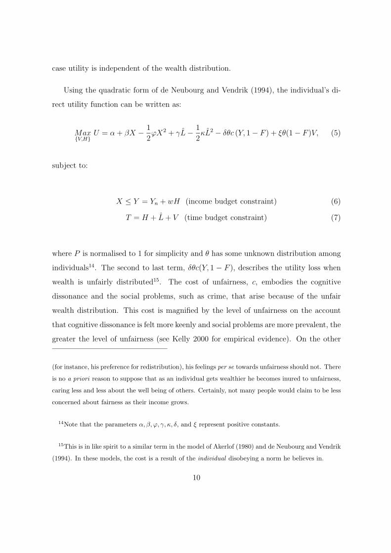
Using the quadratic form of de Neubourg and Vendrik (1994), the individual’s di-
rect utility function can be written as:
Max{V,H}
U = α + βX − 1
2ϕX2 + γL− 1
2κL2 − δθc (Y, 1− F ) + ξθ(1− F )V, (5)
subject to:
X ≤ Y = Yn + wH (income budget constraint) (6)
T = H + L + V (time budget constraint) (7)
where P is normalised to 1 for simplicity and θ has some unknown distribution among
individuals14. The second to last term, δθc(Y, 1 − F ), describes the utility loss when
wealth is unfairly distributed15. The cost of unfairness, c, embodies the cognitive
dissonance and the social problems, such as crime, that arise because of the unfair
wealth distribution. This cost is magnified by the level of unfairness on the account
that cognitive dissonance is felt more keenly and social problems are more prevalent, the
greater the level of unfairness (see Kelly 2000 for empirical evidence). On the other
(for instance, his preference for redistribution), his feelings per se towards unfairness should not. There
is no a priori reason to suppose that as an individual gets wealthier he becomes inured to unfairness,
caring less and less about the well being of others. Certainly, not many people would claim to be less
concerned about fairness as their income grows.
14Note that the parameters α, β, ϕ, γ, κ, δ, and ξ represent positive constants.
15This is in like spirit to a similar term in the model of Akerlof (1980) and de Neubourg and Vendrik
(1994). In these models, the cost is a result of the individual disobeying a norm he believes in.
10
hand, the cost of unfairness is moderated as income rises insofar as the individual
is able to reduce cognitive dissonance by making charitable donations or living in
neighbourhoods where reminders of inequality are fewer. The individual can also limit
exposure to social problems by purchasing insurance for instance, or by investing in
a safer neighbourhood. Therefore, ∂c∂Y
< 0 and ∂c∂F
< 0. The final term represents
the gain in utility from addressing unfairness, which is greater the higher the level of
unfairness16.
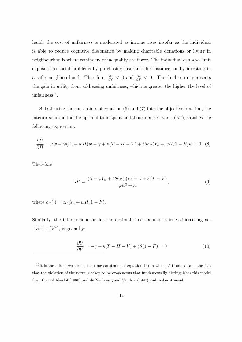
Substituting the constraints of equation (6) and (7) into the objective function, the
interior solution for the optimal time spent on labour market work, (H∗), satisfies the
following expression:
∂U
∂H= βw − ϕ(Yn + wH)w − γ + κ(T −H − V ) + δθcH(Yn + wH, 1− F )w = 0 (8)
Therefore:
H∗ =(β − ϕYn + δθcH(.))w − γ + κ(T − V )
ϕw2 + κ, (9)
where cH(.) = cH(Yn + wH, 1− F ).
Similarly, the interior solution for the optimal time spent on fairness-increasing ac-
tivities, (V ∗), is given by:
∂U
∂V= −γ + κ[T −H − V ] + ξθ(1− F ) = 0 (10)
16It is these last two terms, the time constraint of equation (6) in which V is added, and the fact
that the violation of the norm is taken to be exogeneous that fundamentally distinguishes this model
from that of Akerlof (1980) and de Neubourg and Vendrik (1994) and makes it novel.
11
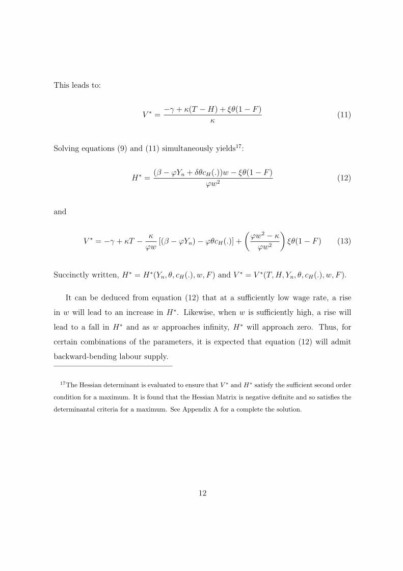
This leads to:
V ∗ =−γ + κ(T −H) + ξθ(1− F )
κ(11)
Solving equations (9) and (11) simultaneously yields17:
H∗ =(β − ϕYn + δθcH(.))w − ξθ(1− F )
ϕw2(12)
and
V ∗ = −γ + κT − κ
ϕw[(β − ϕYn)− ϕθcH(.)] +
(ϕw2 − κ
ϕw2
)ξθ(1− F ) (13)
Succinctly written, H∗ = H∗(Yn, θ, cH(.), w, F ) and V ∗ = V ∗(T, H, Yn, θ, cH(.), w, F ).
It can be deduced from equation (12) that at a sufficiently low wage rate, a rise
in w will lead to an increase in H∗. Likewise, when w is sufficiently high, a rise will
lead to a fall in H∗ and as w approaches infinity, H∗ will approach zero. Thus, for
certain combinations of the parameters, it is expected that equation (12) will admit
backward-bending labour supply.
17The Hessian determinant is evaluated to ensure that V ∗ and H∗ satisfy the sufficient second order
condition for a maximum. It is found that the Hessian Matrix is negative definite and so satisfies the
determinantal criteria for a maximum. See Appendix A for a complete the solution.
12
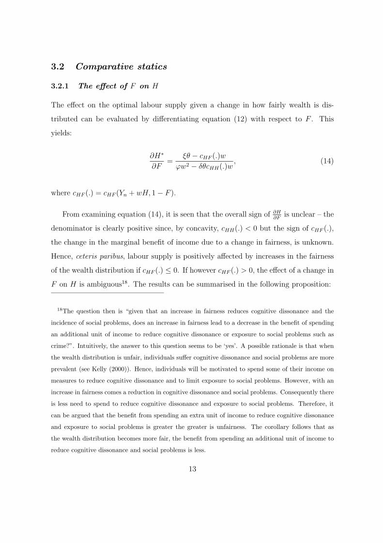
3.2 Comparative statics
3.2.1 The effect of F on H
The effect on the optimal labour supply given a change in how fairly wealth is dis-
tributed can be evaluated by differentiating equation (12) with respect to F . This
yields:
∂H∗
∂F=
ξθ − cHF (.)w
ϕw2 − δθcHH(.)w, (14)
where cHF (.) = cHF (Yn + wH, 1− F ).
From examining equation (14), it is seen that the overall sign of ∂H∂F
is unclear – the
denominator is clearly positive since, by concavity, cHH(.) < 0 but the sign of cHF (.),
the change in the marginal benefit of income due to a change in fairness, is unknown.
Hence, ceteris paribus, labour supply is positively affected by increases in the fairness
of the wealth distribution if cHF (.) ≤ 0. If however cHF (.) > 0, the effect of a change in
F on H is ambiguous18. The results can be summarised in the following proposition:
18The question then is “given that an increase in fairness reduces cognitive dissonance and the
incidence of social problems, does an increase in fairness lead to a decrease in the benefit of spending
an additional unit of income to reduce cognitive dissonance or exposure to social problems such as
crime?”. Intuitively, the answer to this question seems to be ‘yes’. A possible rationale is that when
the wealth distribution is unfair, individuals suffer cognitive dissonance and social problems are more
prevalent (see Kelly (2000)). Hence, individuals will be motivated to spend some of their income on
measures to reduce cognitive dissonance and to limit exposure to social problems. However, with an
increase in fairness comes a reduction in cognitive dissonance and social problems. Consequently there
is less need to spend to reduce cognitive dissonance and exposure to social problems. Therefore, it
can be argued that the benefit from spending an extra unit of income to reduce cognitive dissonance
and exposure to social problems is greater the greater is unfairness. The corollary follows that as
the wealth distribution becomes more fair, the benefit from spending an additional unit of income to
reduce cognitive dissonance and social problems is less.
13
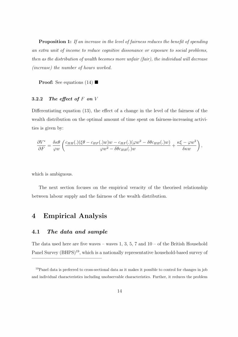
Proposition 1: If an increase in the level of fairness reduces the benefit of spending
an extra unit of income to reduce cognitive dissonance or exposure to social problems,
then as the distribution of wealth becomes more unfair (fair), the individual will decrease
(increase) the number of hours worked.
Proof: See equations (14) �
3.2.2 The effect of F on V
Differentiating equation (13), the effect of a change in the level of the fairness of the
wealth distribution on the optimal amount of time spent on fairness-increasing activi-
ties is given by:
∂V ∗
∂F=
δκθ
ϕw
(cHH(.)(ξθ − cHF (.)w)w − cHF (.)(ϕw2 − δθcHH(.)w)
ϕw2 − δθcHH(.)w+
κξ − ϕw2
δκw
),
which is ambiguous.
The next section focuses on the empirical veracity of the theorised relationship
between labour supply and the fairness of the wealth distribution.
4 Empirical Analysis
4.1 The data and sample
The data used here are five waves – waves 1, 3, 5, 7 and 10 – of the British Household
Panel Survey (BHPS)19, which is a nationally representative household-based survey of
19Panel data is preferred to cross-sectional data as it makes it possible to control for changes in job
and individual characteristics including unobservable characteristics. Further, it reduces the problem
14
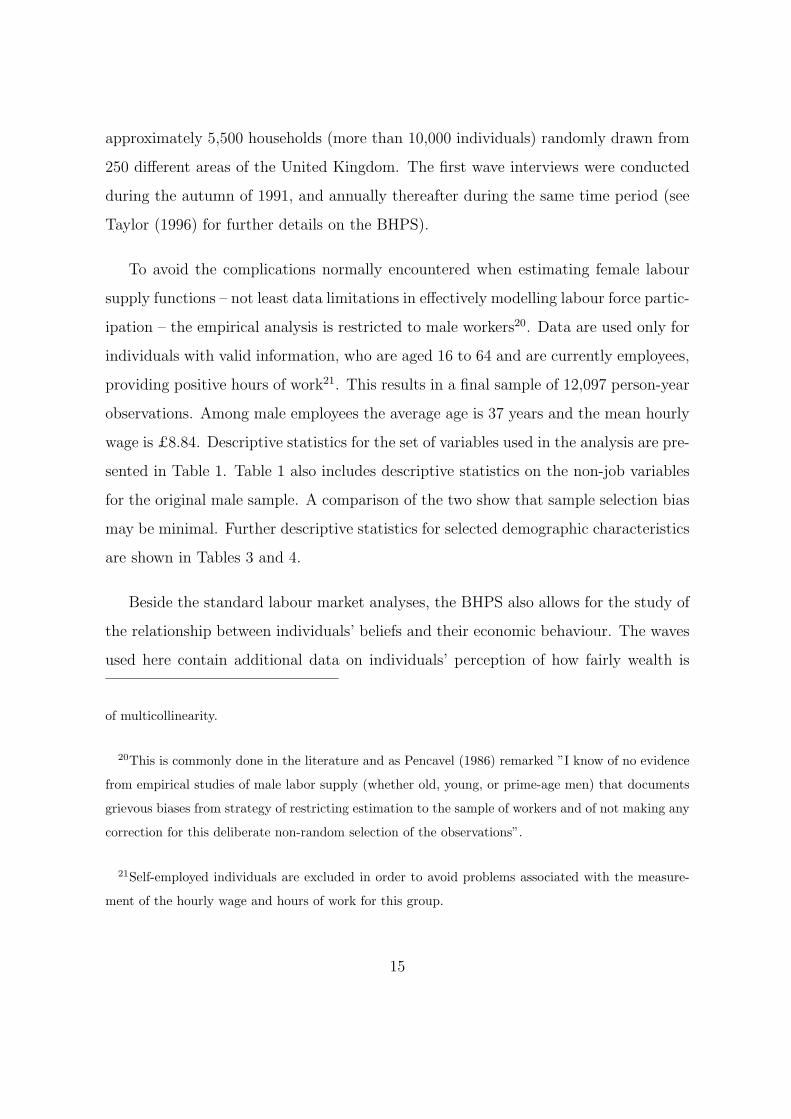
approximately 5,500 households (more than 10,000 individuals) randomly drawn from
250 different areas of the United Kingdom. The first wave interviews were conducted
during the autumn of 1991, and annually thereafter during the same time period (see
Taylor (1996) for further details on the BHPS).
To avoid the complications normally encountered when estimating female labour
supply functions – not least data limitations in effectively modelling labour force partic-
ipation – the empirical analysis is restricted to male workers20. Data are used only for
individuals with valid information, who are aged 16 to 64 and are currently employees,
providing positive hours of work21. This results in a final sample of 12,097 person-year
observations. Among male employees the average age is 37 years and the mean hourly
wage is £8.84. Descriptive statistics for the set of variables used in the analysis are pre-
sented in Table 1. Table 1 also includes descriptive statistics on the non-job variables
for the original male sample. A comparison of the two show that sample selection bias
may be minimal. Further descriptive statistics for selected demographic characteristics
are shown in Tables 3 and 4.
Beside the standard labour market analyses, the BHPS also allows for the study of
the relationship between individuals’ beliefs and their economic behaviour. The waves
used here contain additional data on individuals’ perception of how fairly wealth is
of multicollinearity.
20This is commonly done in the literature and as Pencavel (1986) remarked ”I know of no evidence
from empirical studies of male labor supply (whether old, young, or prime-age men) that documents
grievous biases from strategy of restricting estimation to the sample of workers and of not making any
correction for this deliberate non-random selection of the observations”.
21Self-employed individuals are excluded in order to avoid problems associated with the measure-
ment of the hourly wage and hours of work for this group.
15
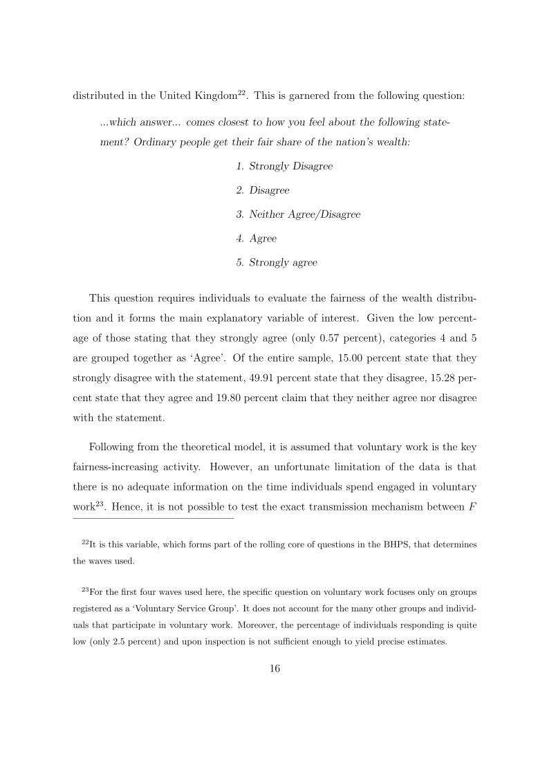
distributed in the United Kingdom22. This is garnered from the following question:
...which answer... comes closest to how you feel about the following state-
ment? Ordinary people get their fair share of the nation’s wealth:
1. Strongly Disagree
2. Disagree
3. Neither Agree/Disagree
4. Agree
5. Strongly agree
This question requires individuals to evaluate the fairness of the wealth distribu-
tion and it forms the main explanatory variable of interest. Given the low percent-
age of those stating that they strongly agree (only 0.57 percent), categories 4 and 5
are grouped together as ‘Agree’. Of the entire sample, 15.00 percent state that they
strongly disagree with the statement, 49.91 percent state that they disagree, 15.28 per-
cent state that they agree and 19.80 percent claim that they neither agree nor disagree
with the statement.
Following from the theoretical model, it is assumed that voluntary work is the key
fairness-increasing activity. However, an unfortunate limitation of the data is that
there is no adequate information on the time individuals spend engaged in voluntary
work23. Hence, it is not possible to test the exact transmission mechanism between F
22It is this variable, which forms part of the rolling core of questions in the BHPS, that determines
the waves used.
23For the first four waves used here, the specific question on voluntary work focuses only on groups
registered as a ‘Voluntary Service Group’. It does not account for the many other groups and individ-
uals that participate in voluntary work. Moreover, the percentage of individuals responding is quite
low (only 2.5 percent) and upon inspection is not sufficient enough to yield precise estimates.
16
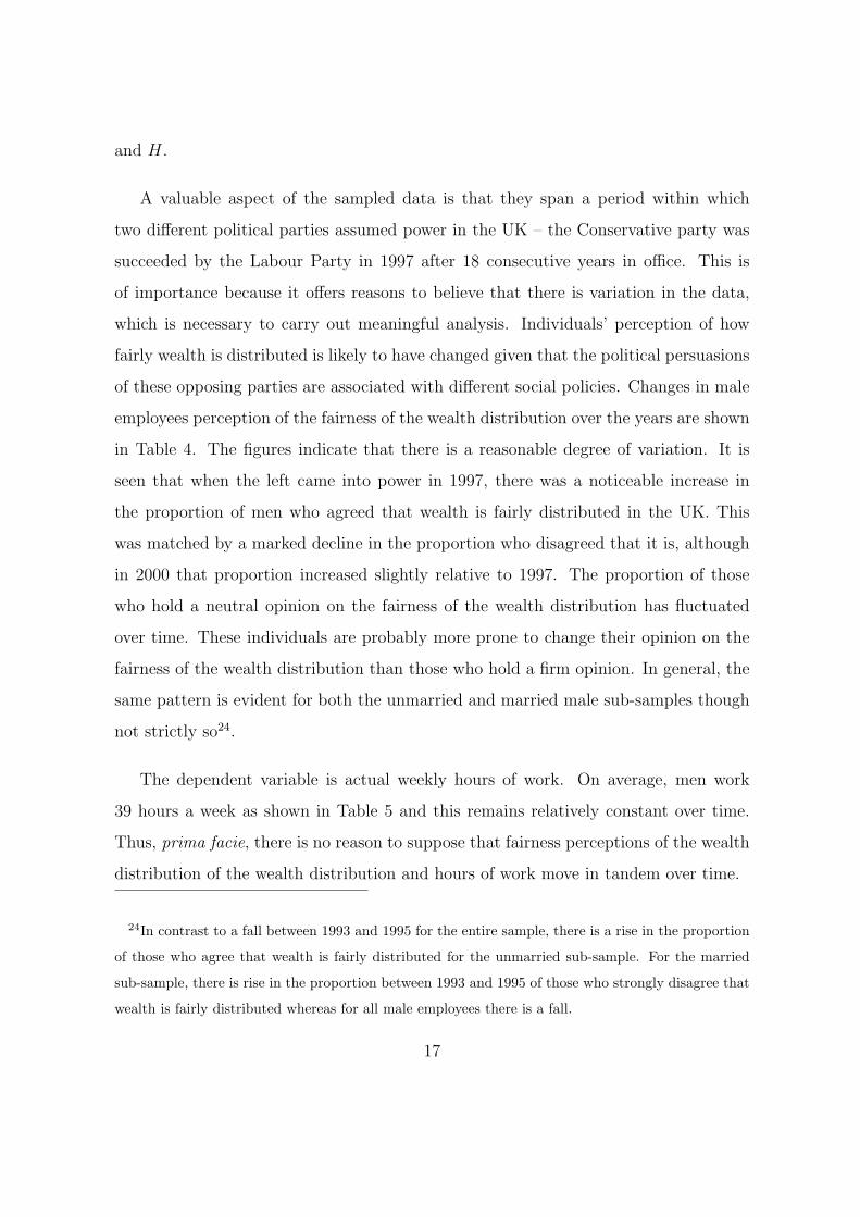
and H.
A valuable aspect of the sampled data is that they span a period within which
two different political parties assumed power in the UK – the Conservative party was
succeeded by the Labour Party in 1997 after 18 consecutive years in office. This is
of importance because it offers reasons to believe that there is variation in the data,
which is necessary to carry out meaningful analysis. Individuals’ perception of how
fairly wealth is distributed is likely to have changed given that the political persuasions
of these opposing parties are associated with different social policies. Changes in male
employees perception of the fairness of the wealth distribution over the years are shown
in Table 4. The figures indicate that there is a reasonable degree of variation. It is
seen that when the left came into power in 1997, there was a noticeable increase in
the proportion of men who agreed that wealth is fairly distributed in the UK. This
was matched by a marked decline in the proportion who disagreed that it is, although
in 2000 that proportion increased slightly relative to 1997. The proportion of those
who hold a neutral opinion on the fairness of the wealth distribution has fluctuated
over time. These individuals are probably more prone to change their opinion on the
fairness of the wealth distribution than those who hold a firm opinion. In general, the
same pattern is evident for both the unmarried and married male sub-samples though
not strictly so24.
The dependent variable is actual weekly hours of work. On average, men work
39 hours a week as shown in Table 5 and this remains relatively constant over time.
Thus, prima facie, there is no reason to suppose that fairness perceptions of the wealth
distribution of the wealth distribution and hours of work move in tandem over time.
24In contrast to a fall between 1993 and 1995 for the entire sample, there is a rise in the proportion
of those who agree that wealth is fairly distributed for the unmarried sub-sample. For the married
sub-sample, there is rise in the proportion between 1993 and 1995 of those who strongly disagree that
wealth is fairly distributed whereas for all male employees there is a fall.
17
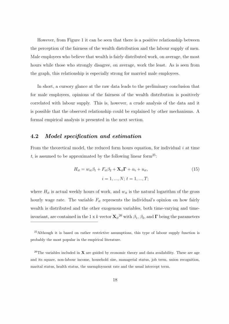
However, from Figure 1 it can be seen that there is a positive relationship between
the perception of the fairness of the wealth distribution and the labour supply of men.
Male employees who believe that wealth is fairly distributed work, on average, the most
hours while those who strongly disagree, on average, work the least. As is seen from
the graph, this relationship is especially strong for married male employees.
In short, a cursory glance at the raw data leads to the preliminary conclusion that
for male employees, opinions of the fairness of the wealth distribution is positively
correlated with labour supply. This is, however, a crude analysis of the data and it
is possible that the observed relationship could be explained by other mechanisms. A
formal empirical analysis is presented in the next section.
4.2 Model specification and estimation
From the theoretical model, the reduced form hours equation, for individual i at time
t, is assumed to be approximated by the following linear form25:
Hit = witβ1 + Fitβ2 + XitΓ + αi + uit, (15)
i = 1, ..., N ; t = 1, ..., T ;
where Hit is actual weekly hours of work, and wit is the natural logarithm of the gross
hourly wage rate. The variable Fit represents the individual’s opinion on how fairly
wealth is distributed and the other exogenous variables, both time-varying and time-
invariant, are contained in the 1 x k vector Xit26 with β1, β2, and Γ being the parameters
25Although it is based on rather restrictive assumptions, this type of labour supply function is
probably the most popular in the empirical literature.
26The variables included in X are guided by economic theory and data availability. These are age
and its square, non-labour income, household size, managerial status, job term, union recognition,
marital status, health status, the unemployment rate and the usual intercept term.
18
to be estimated. The time-invariant random error term, αi, captures the effects of
unobservable individual-specific heterogenous characteristics. The idiosyncratic error
term, given by uit, is assumed to be independently identically distributed (i.i.d) with
mean zero and variance σ2. As is customarily assumed, (u|Zi1, ...,ZiT, αi) = 0, where
Z = [w,F,X].
4.2.1 Unobserved Heterogeneity
An important issue that must be addressed to ensure consistent and efficient parame-
ter estimates is the relationship between the unobserved individual heterogeneity term
and the observed explanatory variables. If αi is arbitrarily correlated with the observed
explanatory variables, a fixed effects estimation approach will yield consistent and ef-
ficient estimates but the GLS (random effects) estimator would be inconsistent. On
the other hand, if E(αi|Z) = E(αi) = 0, that means αi is orthogonal to the observed
explanatory variables, both a random effects estimation and a fixed effects estima-
tion would give consistent and efficient estimates but the within-group (fixed effects)
estimator would be inefficient. Therefore, under the null hypothesis that αi is uncor-
related with the observable explanatory variables, the two estimators should not differ
systematically.
Hausman (1978) proposed a test based on the difference between the two estimators
to determine which of the methods of estimation is most appropriate. To illustrate, let
δFE be the 1 x m vector of within-group estimates on the time-varying observables and
likewise let δRE be the 1 x m vector of GLS estimates on the time-varying observables.
Then, the H statistic is given by
H =[δFE − δRE
]′ [ˆcov(δFE)− ˆcov(δRE)
]−1 [δFE − δRE
](16)
and is distributed χ2(m) where m denotes the degrees of freedom. The terms ˆcov(δFE)
19
and ˆcov(δRE) are consistent estimates of the asymptotic covariance matrices of δFE and
δRE respectively. The implementation of this tests yields χ2(22) = 154.48, which against
the 10 percent critical value of 30.81 leads to a rejection of the random effects model27.
Hence, the analysis employs a fixed effects model.
For the case of the linear fixed effects specification28 this requires transforming
equation (13) by first averaging all variables over t = 1, ..., T to get the cross-section
equation:
Hi = wiβ1 + Fiβ3 + XiΓ + α1i + ui (17)
i = 1, ..., N ; t = 1, ..., T ;
where Hi =1
T
T∑t=1
Hit,
wi =1
T
T∑t=1
wit, Fi =1
T
T∑t=1
Fit,
Xi =1
T
T∑t=1
Xit, and ui =1
T
T∑t=1
uit
Equation (15) is then subtracted from equation (13). This gets rid of the heterogeneity
and gives the fixed effects estimating equation:
27The random effects model is also rejected at the 1 percent and 5 percent significance level.
28It is should borne in mind that as in the random effects specification, the αis are still regarded
as random in the fixed effects linear model (see Mundlak (1978)) but in contrast, they are treated as
parameters to be estimated.
20
Hit − Hi = (wit − wi)β1 + (Fit − Fi)β3 + (Xit − Xi)Γ + (uit − ui) (18)
i = 1, ..., N ; t = 1, ..., T
By using fixed effects estimation, it is possible for the necessary orthogonality condi-
tion to hold (that is, E(αi|Zit) = 0) while still being able to allow for E(αi|Zi1, ...,ZiT )
to be any function of the Zs. This ability to provide a more robust answer to the omit-
ted variables problem vis-a-vis random effects estimation is a very attractive advantage
of fixed effects estimation. Moreover, the problem of sample selection bias is gener-
ally presumed to be less of a concern since αi is removed from the estimating equation
thereby eliminating the drawback of any correlation with uit (see Vella (1998))29. Given
this and the information in Table 1, which shows a very close similarity between the
descriptive statistics for the sample of male employees and the original male sample,
it will be assumed that sample selection bias is not a cause for concern here.
4.2.2 The endogeneity of wages
It is widely acknowledged that wages may be endogenous in an hours equation. Conse-
quently, the ordinary least squares (OLS) estimate will be biased and the consistency
of the other estimators may be affected. Here, two reasons for this possible endogeneity
are that: (1) hourly wages is not reported directly and must be derived by dividing
labour income by hours worked. Therefore, any measurement errors in hours may give
rise to what is referred to by Borjas (1980) as a ‘division bias’. In other words, a
downward bias to the estimated wage coefficient as a result of spurious correlation be-
tween hourly wage, wit and the error term, uit, in the hours equation may emerge. (2)
unobservable characteristics that influence wages may be correlated with unobservable
29Nonetheless, if the idiosyncratic error term in a labour force participation equation is correlated
with uit, selectivity bias will not necessarily be mitigated by fixed effects estimation.
21
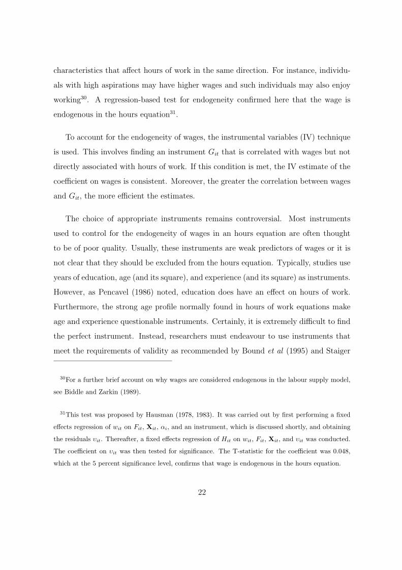
characteristics that affect hours of work in the same direction. For instance, individu-
als with high aspirations may have higher wages and such individuals may also enjoy
working30. A regression-based test for endogeneity confirmed here that the wage is
endogenous in the hours equation31.
To account for the endogeneity of wages, the instrumental variables (IV) technique
is used. This involves finding an instrument Git that is correlated with wages but not
directly associated with hours of work. If this condition is met, the IV estimate of the
coefficient on wages is consistent. Moreover, the greater the correlation between wages
and Git, the more efficient the estimates.
The choice of appropriate instruments remains controversial. Most instruments
used to control for the endogeneity of wages in an hours equation are often thought
to be of poor quality. Usually, these instruments are weak predictors of wages or it is
not clear that they should be excluded from the hours equation. Typically, studies use
years of education, age (and its square), and experience (and its square) as instruments.
However, as Pencavel (1986) noted, education does have an effect on hours of work.
Furthermore, the strong age profile normally found in hours of work equations make
age and experience questionable instruments. Certainly, it is extremely difficult to find
the perfect instrument. Instead, researchers must endeavour to use instruments that
meet the requirements of validity as recommended by Bound et al (1995) and Staiger
30For a further brief account on why wages are considered endogenous in the labour supply model,
see Biddle and Zarkin (1989).
31This test was proposed by Hausman (1978, 1983). It was carried out by first performing a fixed
effects regression of wit on Fit, Xit, αi, and an instrument, which is discussed shortly, and obtaining
the residuals υit. Thereafter, a fixed effects regression of Hit on wit, Fit, Xit, and υit was conducted.
The coefficient on υit was then tested for significance. The T-statistic for the coefficient was 0.048,
which at the 5 percent significance level, confirms that wage is endogenous in the hours equation.
22
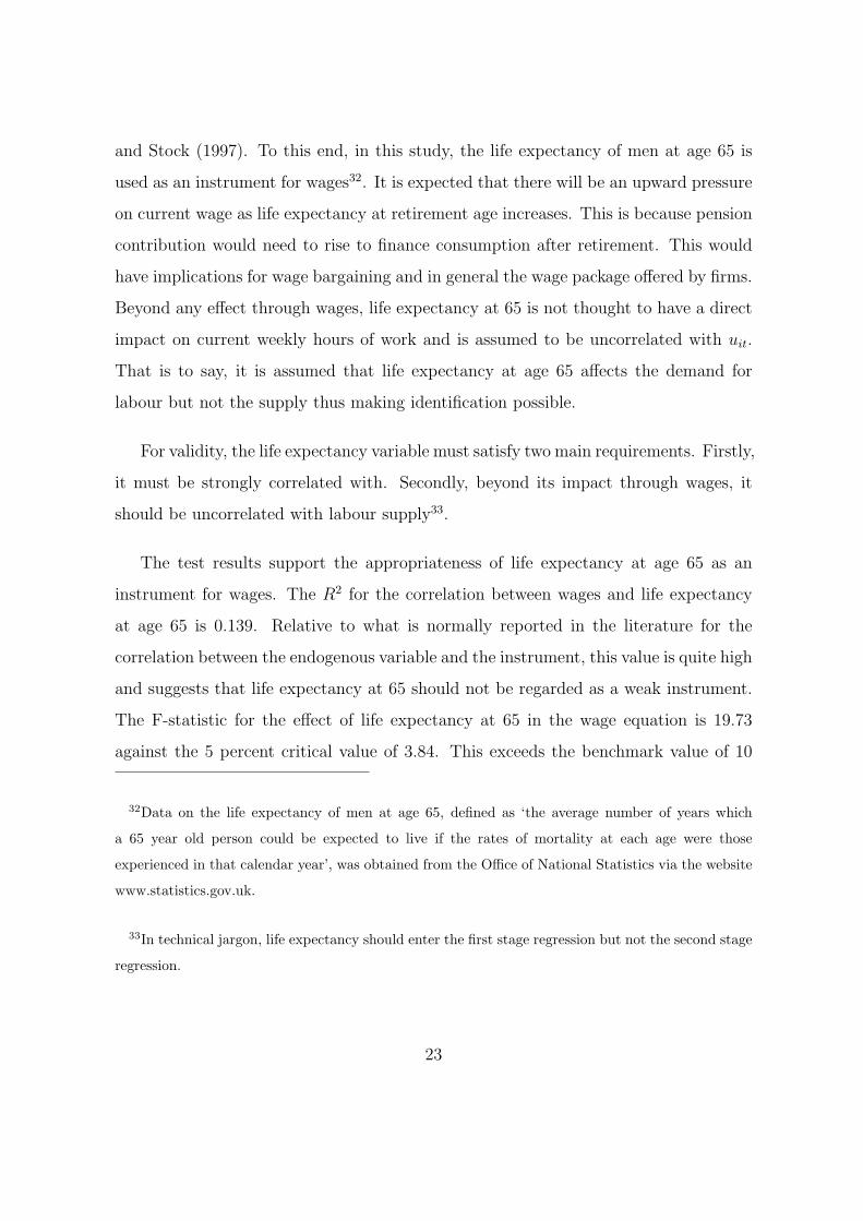
and Stock (1997). To this end, in this study, the life expectancy of men at age 65 is
used as an instrument for wages32. It is expected that there will be an upward pressure
on current wage as life expectancy at retirement age increases. This is because pension
contribution would need to rise to finance consumption after retirement. This would
have implications for wage bargaining and in general the wage package offered by firms.
Beyond any effect through wages, life expectancy at 65 is not thought to have a direct
impact on current weekly hours of work and is assumed to be uncorrelated with uit.
That is to say, it is assumed that life expectancy at age 65 affects the demand for
labour but not the supply thus making identification possible.
For validity, the life expectancy variable must satisfy two main requirements. Firstly,
it must be strongly correlated with. Secondly, beyond its impact through wages, it
should be uncorrelated with labour supply33.
The test results support the appropriateness of life expectancy at age 65 as an
instrument for wages. The R2 for the correlation between wages and life expectancy
at age 65 is 0.139. Relative to what is normally reported in the literature for the
correlation between the endogenous variable and the instrument, this value is quite high
and suggests that life expectancy at 65 should not be regarded as a weak instrument.
The F-statistic for the effect of life expectancy at 65 in the wage equation is 19.73
against the 5 percent critical value of 3.84. This exceeds the benchmark value of 10
32Data on the life expectancy of men at age 65, defined as ‘the average number of years which
a 65 year old person could be expected to live if the rates of mortality at each age were those
experienced in that calendar year’, was obtained from the Office of National Statistics via the website
www.statistics.gov.uk.
33In technical jargon, life expectancy should enter the first stage regression but not the second stage
regression.
23
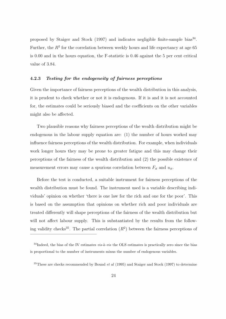
proposed by Staiger and Stock (1997) and indicates negligible finite-sample bias34.
Further, the R2 for the correlation between weekly hours and life expectancy at age 65
is 0.00 and in the hours equation, the F-statistic is 0.46 against the 5 per cent critical
value of 3.84.
4.2.3 Testing for the endogeneity of fairness perceptions
Given the importance of fairness perceptions of the wealth distribution in this analysis,
it is prudent to check whether or not it is endogenous. If it is and it is not accounted
for, the estimates could be seriously biased and the coefficients on the other variables
might also be affected.
Two plausible reasons why fairness perceptions of the wealth distribution might be
endogenous in the labour supply equation are: (1) the number of hours worked may
influence fairness perceptions of the wealth distribution. For example, when individuals
work longer hours they may be prone to greater fatigue and this may change their
perceptions of the fairness of the wealth distribution and (2) the possible existence of
measurement errors may cause a spurious correlation between Fit and uit.
Before the test is conducted, a suitable instrument for fairness perceptions of the
wealth distribution must be found. The instrument used is a variable describing indi-
viduals’ opinion on whether ‘there is one law for the rich and one for the poor’. This
is based on the assumption that opinions on whether rich and poor individuals are
treated differently will shape perceptions of the fairness of the wealth distribution but
will not affect labour supply. This is substantiated by the results from the follow-
ing validity checks35. The partial correlation (R2) between the fairness perceptions of
34Indeed, the bias of the IV estimates vis-a-vis the OLS estimates is practically zero since the bias
is proportional to the number of instruments minus the number of endogenous variables.
35These are checks recommended by Bound et al (1995) and Staiger and Stock (1997) to determine
24
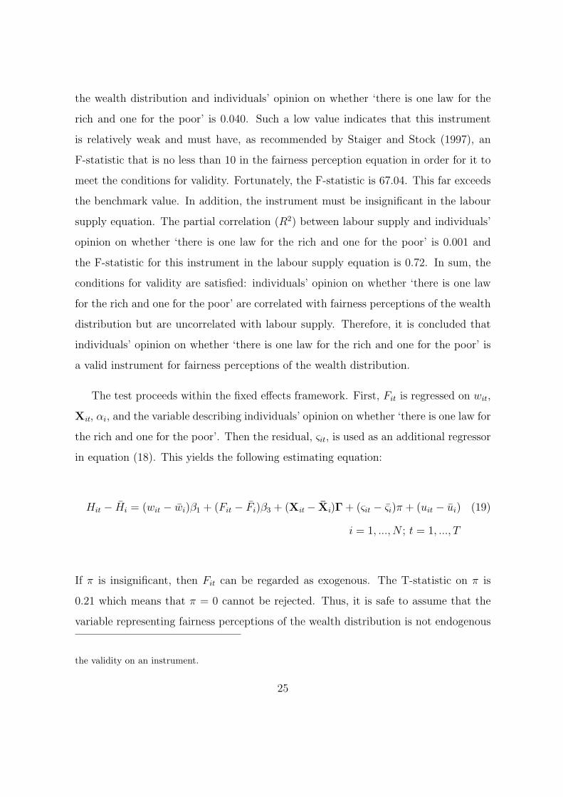
the wealth distribution and individuals’ opinion on whether ‘there is one law for the
rich and one for the poor’ is 0.040. Such a low value indicates that this instrument
is relatively weak and must have, as recommended by Staiger and Stock (1997), an
F-statistic that is no less than 10 in the fairness perception equation in order for it to
meet the conditions for validity. Fortunately, the F-statistic is 67.04. This far exceeds
the benchmark value. In addition, the instrument must be insignificant in the labour
supply equation. The partial correlation (R2) between labour supply and individuals’
opinion on whether ‘there is one law for the rich and one for the poor’ is 0.001 and
the F-statistic for this instrument in the labour supply equation is 0.72. In sum, the
conditions for validity are satisfied: individuals’ opinion on whether ‘there is one law
for the rich and one for the poor’ are correlated with fairness perceptions of the wealth
distribution but are uncorrelated with labour supply. Therefore, it is concluded that
individuals’ opinion on whether ‘there is one law for the rich and one for the poor’ is
a valid instrument for fairness perceptions of the wealth distribution.
The test proceeds within the fixed effects framework. First, Fit is regressed on wit,
Xit, αi, and the variable describing individuals’ opinion on whether ‘there is one law for
the rich and one for the poor’. Then the residual, ςit, is used as an additional regressor
in equation (18). This yields the following estimating equation:
Hit − Hi = (wit − wi)β1 + (Fit − Fi)β3 + (Xit − Xi)Γ + (ςit − ςi)π + (uit − ui) (19)
i = 1, ..., N ; t = 1, ..., T
If π is insignificant, then Fit can be regarded as exogenous. The T-statistic on π is
0.21 which means that π = 0 cannot be rejected. Thus, it is safe to assume that the
variable representing fairness perceptions of the wealth distribution is not endogenous
the validity on an instrument.
25
in the hours equation and that the possible problems of time-varying unobservables
and measurement error are not cause for concern.
4.3 Results
4.3.1 Main Results
For comparative purposes, the OLS results for equation (16) are presented along with
the IV estimates.
OLS within-group Estimates
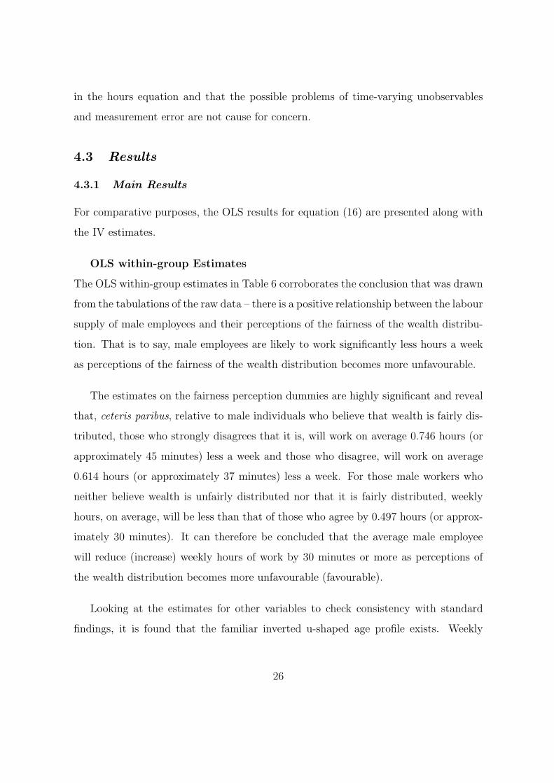
The OLS within-group estimates in Table 6 corroborates the conclusion that was drawn
from the tabulations of the raw data – there is a positive relationship between the labour
supply of male employees and their perceptions of the fairness of the wealth distribu-
tion. That is to say, male employees are likely to work significantly less hours a week
as perceptions of the fairness of the wealth distribution becomes more unfavourable.
The estimates on the fairness perception dummies are highly significant and reveal
that, ceteris paribus, relative to male individuals who believe that wealth is fairly dis-
tributed, those who strongly disagrees that it is, will work on average 0.746 hours (or
approximately 45 minutes) less a week and those who disagree, will work on average
0.614 hours (or approximately 37 minutes) less a week. For those male workers who
neither believe wealth is unfairly distributed nor that it is fairly distributed, weekly
hours, on average, will be less than that of those who agree by 0.497 hours (or approx-
imately 30 minutes). It can therefore be concluded that the average male employee
will reduce (increase) weekly hours of work by 30 minutes or more as perceptions of
the wealth distribution becomes more unfavourable (favourable).
Looking at the estimates for other variables to check consistency with standard
findings, it is found that the familiar inverted u-shaped age profile exists. Weekly
26
hours of work rise with age at about one hour and a quarter a week but at a decreasing
rate reaching a peak at age 44 and then declining thereafter36.
For both wages and non-labour income there is a negative relationship with hours
of work. Intuitively, as non-labour income increases, the need for working diminishes
insofar as the individual is able to maintain consumption by working less hours and
will wish to do so since working tends to reduce utility. On the contrary, wages would
normally be expected to be positively related to hours of work. However, it is not
unusual in empirical studies of labour supply to find that log wage enters the hours
equation negatively as it does here. One explanation is that individuals are on the
backward bending portion of their labour supply curve. Another could be that the
endogeneity of wages in the hours equation may be the cause of this downward bias in
the estimate. This possibility is addressed by looking at the IV results.
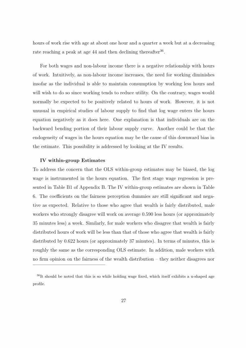
IV within-group Estimates
To address the concern that the OLS within-group estimates may be biased, the log
wage is instrumented in the hours equation. The first stage wage regression is pre-
sented in Table B1 of Appendix B. The IV within-group estimates are shown in Table
6. The coefficients on the fairness perception dummies are still significant and nega-
tive as expected. Relative to those who agree that wealth is fairly distributed, male
workers who strongly disagree will work on average 0.590 less hours (or approximately
35 minutes less) a week. Similarly, for male workers who disagree that wealth is fairly
distributed hours of work will be less than that of those who agree that wealth is fairly
distributed by 0.622 hours (or approximately 37 minutes). In terms of minutes, this is
roughly the same as the corresponding OLS estimate. In addition, male workers with
no firm opinion on the fairness of the wealth distribution – they neither disagrees nor
36It should be noted that this is so while holding wage fixed, which itself exhibits a u-shaped age
profile.
27
agrees that wealth is fairly distributed – can be expected to work, on average, 0.521
hours (31 minutes) less a week than those who believe that wealth is fairly distributed.
This too, in terms of minutes, is very close to the corresponding OLS estimate.
There is a slight suggestion from the IV estimates that weekly hours of work do
not decline continuously as perceptions of the wealth distribution becomes successively
unfavourable. It can be seen that compared to those who agree that wealth is fairly
distributed, male employees who disagree will reduce weekly hours by 2 minutes more
than those who strongly disagree. However, this difference is quite small and possibly
insignificant.
In sum, the IV within-group estimates lead to the same conclusion as the OLS
within-group estimates, which is that the average male employee will decrease (in-
crease) his weekly hours of work as the wealth distribution becomes more unfair (fair)
by as much as 30 minutes or more.
In the case of the other variables, it is found that the coefficient on age and age
squared have the same sign as those in the OLS estimation but they are insignificant.
Non-labour income on the other hand still has a negative and significant influence on
weekly hours of work. Not surprising, the IV estimate of log hourly wage is greater
than the OLS estimate and has the expected positive sign but it is insignificant.
In general, the IV standard errors are much greater than the OLS standard errors.
This is not uncommon with IV estimation. Nonetheless, the estimates are still highly
precise and are consistent whereas, despite being more precise, the OLS estimates are
inconsistent.
28
4.3.2 Additional Results
The sample is split into unmarried37 and married male employees to determine whether
there are marked differences between the two38. Arguably, unmarried individuals may
have less home commitments and hence more flexibility with respect to their weekly
hours of work. Therefore, hours of work of unmarried individuals may be more respon-
sive to perceptions of how fairly wealth is distributed. IV estimates are presented in
Table 7 and the first stage wage regressions are shown in Table B2 of Appendix B.
To begin, it is important to check that life expectancy at age 65 remains a valid
instrument for wages in each subsample. The R2 for the correlation between wages and
life expectancy at age 65 is 0.216 for unmarried male employees and 0.077 for married
employees. Based on this, it appears that life expectancy may be a weak instrument
in the case of married male employees but not so for unmarried male employees.
Given the weak correlation between life expectancy at age 65 and log hourly wage in
the subsample of married male employees, a small correlation between life expectancy
at age 65 and weekly hours can give rise to a larger inconsistency in the IV estimates
compared to the OLS estimates for this group. Consequently, unlike for unmarried
male employees, it is necessary to check that the F-statistic on life expectancy at
37Unmarried individuals are those who are either separated, divorced, widowed, or have never
married.
38Age subsamples were also considered (<25, 25–34, 35–44, 45–54, ≥55) and no strong evidence
that age moderates the impact of fairness perceptions on labour supply behaviour was found. The
subsamples were quite small but this was again supported by the insignificance of the interactions
between age and fairness perceptions for the entire sample. Interactions between wage and the fairness
perception dummies were also tested for significance. The results revealed that the impact of fairness
perceptions on labour supply is not dependent on wages. Given the insignificance of these results,
they are not reported here.
29
age 65 in the hourly wage equation for married male employees is no less than the
benchmark value of 10 suggested by Staiger and Stock (1997). For the subsample of
married male employees, the F-statistic is 15.48. This implies negligible finite sample
bias39. In the case of unmarried male employees, the F-statistic is 1.95. Since the
correlation between life expectancy at age 65 and log hourly wage is relatively high,
finite sample bias may not be a significant problem40. It can therefore be concluded
that it is possible for reliable conclusion to be drawn from the IV estimates in both
the subsamples of unmarried and married male employees.
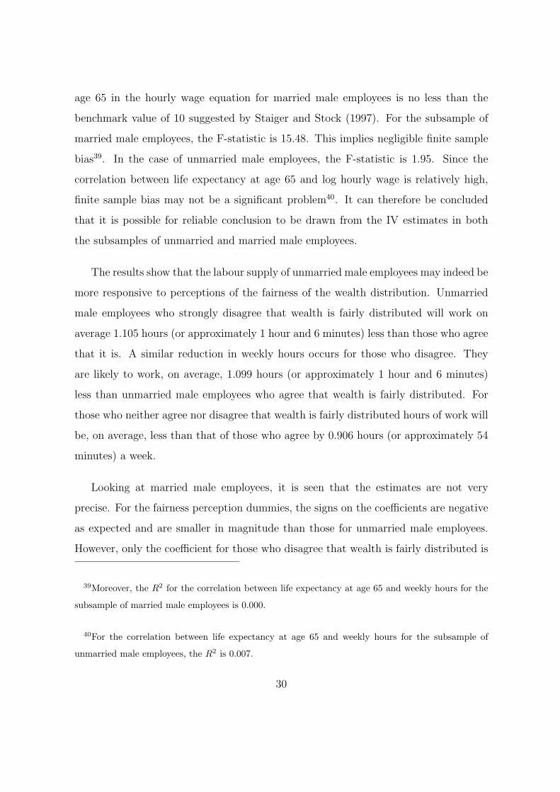
The results show that the labour supply of unmarried male employees may indeed be
more responsive to perceptions of the fairness of the wealth distribution. Unmarried
male employees who strongly disagree that wealth is fairly distributed will work on
average 1.105 hours (or approximately 1 hour and 6 minutes) less than those who agree
that it is. A similar reduction in weekly hours occurs for those who disagree. They
are likely to work, on average, 1.099 hours (or approximately 1 hour and 6 minutes)
less than unmarried male employees who agree that wealth is fairly distributed. For
those who neither agree nor disagree that wealth is fairly distributed hours of work will
be, on average, less than that of those who agree by 0.906 hours (or approximately 54
minutes) a week.
Looking at married male employees, it is seen that the estimates are not very
precise. For the fairness perception dummies, the signs on the coefficients are negative
as expected and are smaller in magnitude than those for unmarried male employees.
However, only the coefficient for those who disagree that wealth is fairly distributed is
39Moreover, the R2 for the correlation between life expectancy at age 65 and weekly hours for the
subsample of married male employees is 0.000.
40For the correlation between life expectancy at age 65 and weekly hours for the subsample of
unmarried male employees, the R2 is 0.007.
30
significant and this is so only at the 10 percent level. According to the estimate, when
compared to those who agree that wealth is fairly distributed, married male employees
who disagree, work on average, 0.566 hours (or approximately 34 minutes) less a week.
Taken together, the findings show that there are important regularities in the data
that are consistent with a positive relationship between labour supply and fairness
perceptions of the wealth distribution.
5 Conclusions
The literature has focused primarily on how the violation of a social norm affects the
economic behaviour of the individual when the individual is the one in violation of the
norm or the target of the violation. Little is known of how the behaviour of individuals
respond to a more global violation of a social norm. That is, the violation of a norm
in cases where the individual is not necessarily directly affected.
Insofar as individuals wish to maintain the norm of fairness in society and suffer
a loss of psychic income whenever the norm of fairness is violated, it is likely that an
unfair wealth distribution will motivate them to engage in fairness-increasing activities
even though they are not themselves directly affected. The prevalence of altruistic
behaviour such as donations and voluntary work attests to individual’s concern for the
well-being of others. Interestingly, survey evidence indicate that voluntary work has
increased alongside increasing wealth inequality.
This paper sets out to determine whether individuals overall concern for fairness
in society influences their labour market behaviour. To this end, a theoretical model
was developed to explain how the fairness of the wealth distribution may affect the
labour supply decision of individuals. It is argued that unfairness in society motivates
individuals to engage in voluntary activities, which draw time away from labour market
31
work. Consequently, it is proposed that labour supply will fall as the wealth distribution
becomes more unfair.
This hypothesis is supported by the empirical findings. It is found that individual
labour supply is positively related to the fairness of the wealth distribution. Using
a fixed effects estimation method and controlling for the endogeneity of wages, the
results reveal that, on average, male employees who believe that wealth is not fairly
distributed or who hold no firm opinion as to whether or not wealth is fairly distributed
work about half an hour less a week than those who believe that it is.
Looking only at unmarried male employees, it is found that, on average, the re-
duction in hours is almost double that for the entire sample of male employees. When
married male employees are considered, it is found that only those who disagree that
wealth is fairly distributed relative to those who agree, that have a statistically signif-
icant reduction in weekly hours. In this case, the reduction is similar to that found for
the entire sample of male employees.
One implication of the results is that, ceteris paribus, if wealth becomes more
unfairly distributed, productivity, as measured by the number of hours spent on labour
market work, will be adversely affected. In this way, the results are suggestive as to
why more egalitarian societies may enjoy higher productivity levels than less egalitarian
societies.
From a policy point of view, the recommendation is simple. To increase productivity
levels the government should seek to achieve a fair distribution of wealth.
32

Figure 1: Average weekly hours and fairness perceptions of the wealth distribution.
33
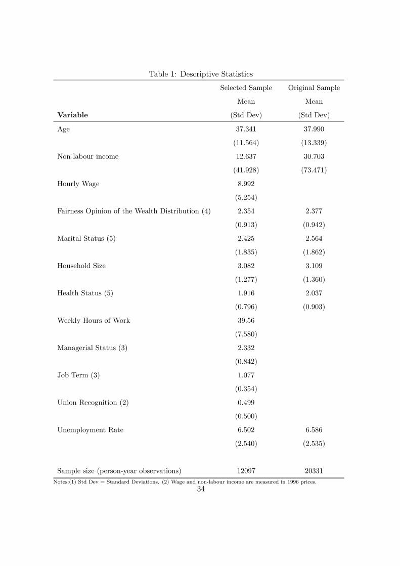
Table 1: Descriptive Statistics
Selected Sample Original Sample
Mean Mean
Variable (Std Dev) (Std Dev)
Age 37.341 37.990
(11.564) (13.339)
Non-labour income 12.637 30.703
(41.928) (73.471)
Hourly Wage 8.992
(5.254)
Fairness Opinion of the Wealth Distribution (4) 2.354 2.377
(0.913) (0.942)
Marital Status (5) 2.425 2.564
(1.835) (1.862)
Household Size 3.082 3.109
(1.277) (1.360)
Health Status (5) 1.916 2.037
(0.796) (0.903)
Weekly Hours of Work 39.56
(7.580)
Managerial Status (3) 2.332
(0.842)
Job Term (3) 1.077
(0.354)
Union Recognition (2) 0.499
(0.500)
Unemployment Rate 6.502 6.586
(2.540) (2.535)
Sample size (person-year observations) 12097 20331Notes:(1) Std Dev = Standard Deviations. (2) Wage and non-labour income are measured in 1996 prices.
34
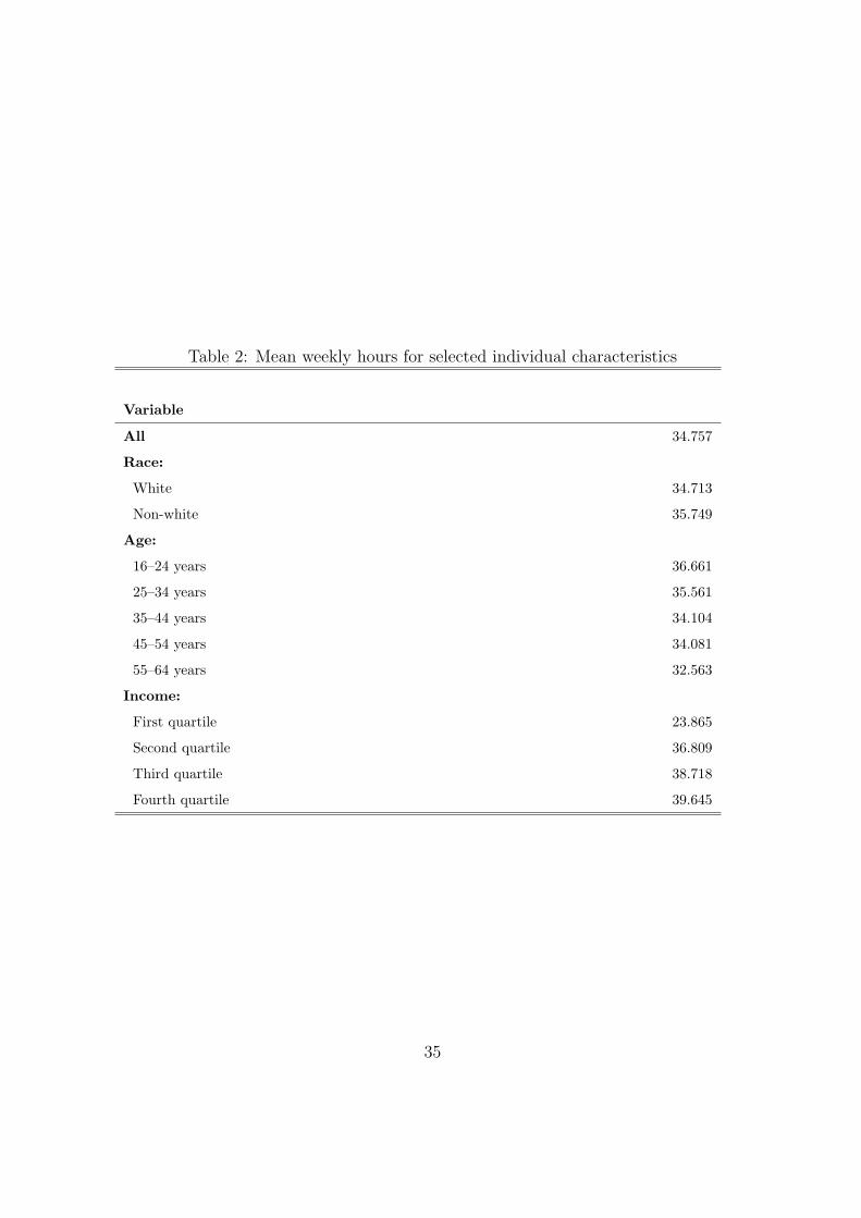
Table 2: Mean weekly hours for selected individual characteristics
Variable
All 34.757
Race:
White 34.713
Non-white 35.749
Age:
16–24 years 36.661
25–34 years 35.561
35–44 years 34.104
45–54 years 34.081
55–64 years 32.563
Income:
First quartile 23.865
Second quartile 36.809
Third quartile 38.718
Fourth quartile 39.645
35

Table 3: Mean weekly hours by fairness perceptions of the wealth distribution
Variable Strongly disagree Disagree Neither Disagree/Agree Agree
All 35.085 34.551 34.573 35.496
Race:
White 35.045 34.517 34.520 35.433
Non-white 36.476 35.395 35.392 36.363
Age:
16–24 years 37.003 36.475 36.588 37.135
25–34 years 35.693 35.396 35.331 36.527
35–44 years 34.546 33.920 33.202 35.763
45–54 years 34.577 33.945 33.602 34.626
55–64 years 34.240 32.504 32.055 31.578
Income:
First quartile 24.450 23.716 23.766 24.011
Second quartile 37.292 36.588 36.612 37.461
Third quartile 38.880 38.585 38.418 39.602
Fourth quartile 39.116 39.556 39.527 40.497
36
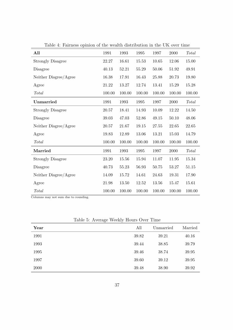
Table 4: Fairness opinion of the wealth distribution in the UK over time
All 1991 1993 1995 1997 2000 Total
Strongly Disagree 22.27 16.61 15.53 10.65 12.06 15.00
Disagree 40.13 52.21 55.29 50.06 51.92 49.91
Neither Disgree/Agree 16.38 17.91 16.43 25.88 20.73 19.80
Agree 21.22 13.27 12.74 13.41 15.29 15.28
Total 100.00 100.00 100.00 100.00 100.00 100.00
Unmarried 1991 1993 1995 1997 2000 Total
Strongly Disagree 20.57 18.41 14.93 10.09 12.22 14.50
Disagree 39.03 47.03 52.86 49.15 50.10 48.06
Neither Disgree/Agree 20.57 21.67 19.15 27.55 22.65 22.65
Agree 19.83 12.89 13.06 13.21 15.03 14.79
Total 100.00 100.00 100.00 100.00 100.00 100.00
Married 1991 1993 1995 1997 2000 Total
Strongly Disagree 23.20 15.56 15.94 11.07 11.95 15.34
Disagree 40.73 55.23 56.93 50.75 53.27 51.15
Neither Disgree/Agree 14.09 15.72 14.61 24.63 19.31 17.90
Agree 21.98 13.50 12.52 13.56 15.47 15.61
Total 100.00 100.00 100.00 100.00 100.00 100.00Columns may not sum due to rounding.
Table 5: Average Weekly Hours Over Time
Year All Unmarried Married
1991 39.82 39.21 40.16
1993 39.44 38.85 39.79
1995 39.46 38.74 39.95
1997 39.60 39.12 39.95
2000 39.48 38.90 39.92
37
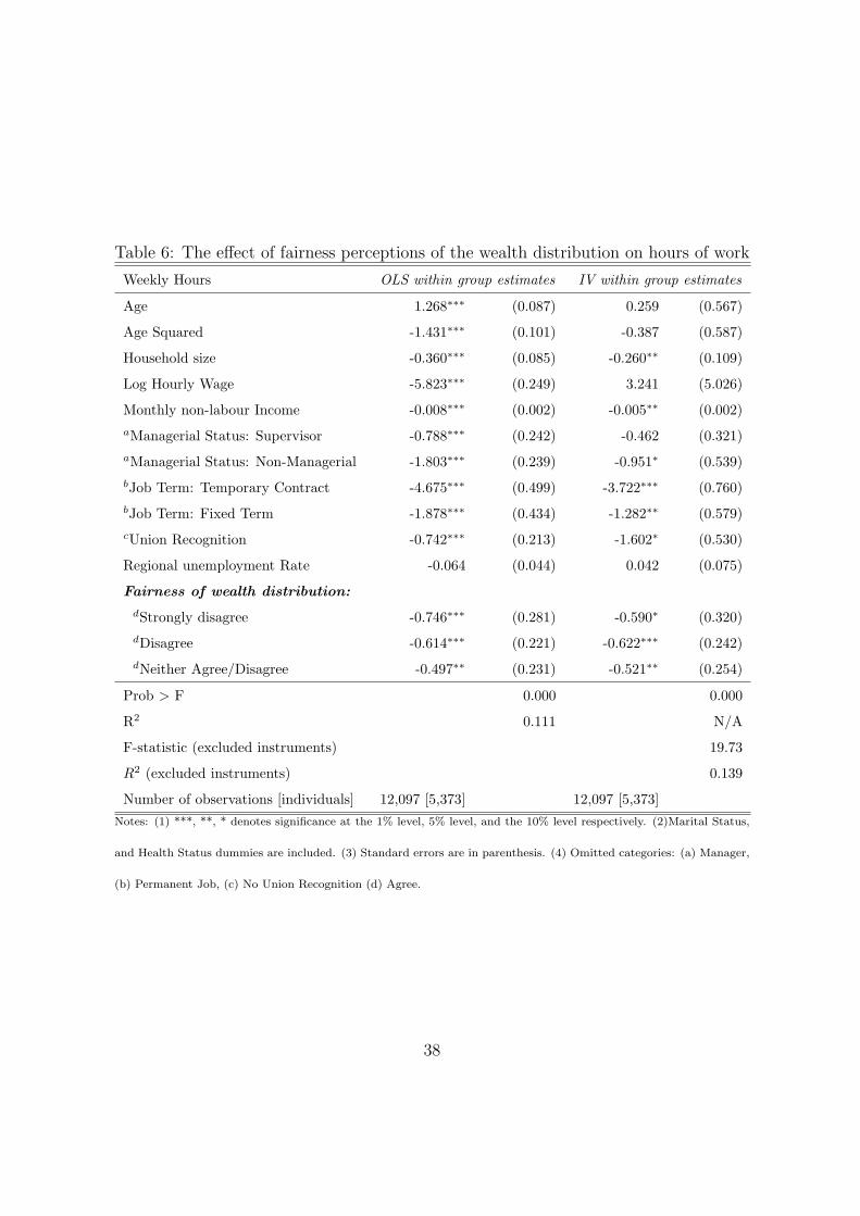
Table 6: The effect of fairness perceptions of the wealth distribution on hours of work
Weekly Hours OLS within group estimates IV within group estimates
Age 1.268∗∗∗ (0.087) 0.259 (0.567)
Age Squared -1.431∗∗∗ (0.101) -0.387 (0.587)
Household size -0.360∗∗∗ (0.085) -0.260∗∗ (0.109)
Log Hourly Wage -5.823∗∗∗ (0.249) 3.241 (5.026)
Monthly non-labour Income -0.008∗∗∗ (0.002) -0.005∗∗ (0.002)aManagerial Status: Supervisor -0.788∗∗∗ (0.242) -0.462 (0.321)aManagerial Status: Non-Managerial -1.803∗∗∗ (0.239) -0.951∗ (0.539)bJob Term: Temporary Contract -4.675∗∗∗ (0.499) -3.722∗∗∗ (0.760)bJob Term: Fixed Term -1.878∗∗∗ (0.434) -1.282∗∗ (0.579)cUnion Recognition -0.742∗∗∗ (0.213) -1.602∗ (0.530)
Regional unemployment Rate -0.064 (0.044) 0.042 (0.075)
Fairness of wealth distribution:
dStrongly disagree -0.746∗∗∗ (0.281) -0.590∗ (0.320)dDisagree -0.614∗∗∗ (0.221) -0.622∗∗∗ (0.242)dNeither Agree/Disagree -0.497∗∗ (0.231) -0.521∗∗ (0.254)
Prob > F 0.000 0.000
R2 0.111 N/A
F-statistic (excluded instruments) 19.73
R2 (excluded instruments) 0.139
Number of observations [individuals] 12,097 [5,373] 12,097 [5,373]Notes: (1) ***, **, * denotes significance at the 1% level, 5% level, and the 10% level respectively. (2)Marital Status,
and Health Status dummies are included. (3) Standard errors are in parenthesis. (4) Omitted categories: (a) Manager,
(b) Permanent Job, (c) No Union Recognition (d) Agree.
38
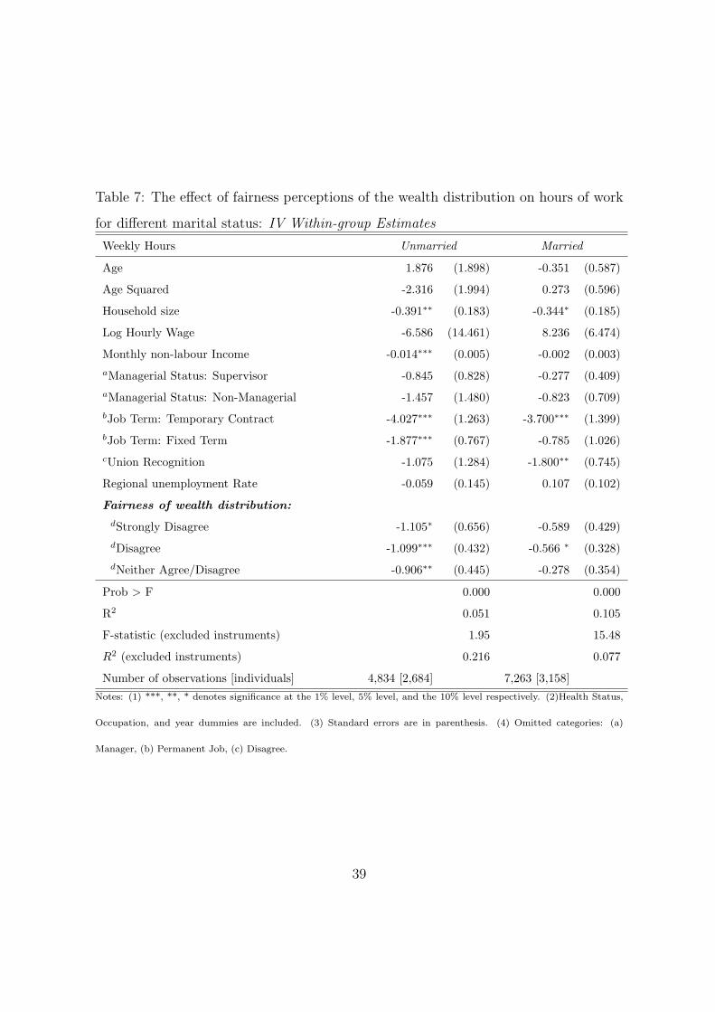
Table 7: The effect of fairness perceptions of the wealth distribution on hours of work
for different marital status: IV Within-group Estimates
Weekly Hours Unmarried Married
Age 1.876 (1.898) -0.351 (0.587)
Age Squared -2.316 (1.994) 0.273 (0.596)
Household size -0.391∗∗ (0.183) -0.344∗ (0.185)
Log Hourly Wage -6.586 (14.461) 8.236 (6.474)
Monthly non-labour Income -0.014∗∗∗ (0.005) -0.002 (0.003)aManagerial Status: Supervisor -0.845 (0.828) -0.277 (0.409)aManagerial Status: Non-Managerial -1.457 (1.480) -0.823 (0.709)bJob Term: Temporary Contract -4.027∗∗∗ (1.263) -3.700∗∗∗ (1.399)bJob Term: Fixed Term -1.877∗∗∗ (0.767) -0.785 (1.026)cUnion Recognition -1.075 (1.284) -1.800∗∗ (0.745)
Regional unemployment Rate -0.059 (0.145) 0.107 (0.102)
Fairness of wealth distribution:
dStrongly Disagree -1.105∗ (0.656) -0.589 (0.429)dDisagree -1.099∗∗∗ (0.432) -0.566 ∗ (0.328)dNeither Agree/Disagree -0.906∗∗ (0.445) -0.278 (0.354)
Prob > F 0.000 0.000
R2 0.051 0.105
F-statistic (excluded instruments) 1.95 15.48
R2 (excluded instruments) 0.216 0.077
Number of observations [individuals] 4,834 [2,684] 7,263 [3,158]Notes: (1) ***, **, * denotes significance at the 1% level, 5% level, and the 10% level respectively. (2)Health Status,
Occupation, and year dummies are included. (3) Standard errors are in parenthesis. (4) Omitted categories: (a)
Manager, (b) Permanent Job, (c) Disagree.
39
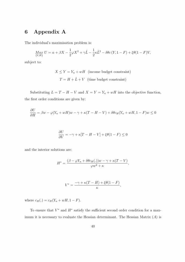
6 Appendix A
The individual’s maximisation problem is:
Max{V,H}
U = α + βX − 1
2ϕX2 + γL− 1
2κL2 − δθc (Y, 1− F ) + ξθ(1− F )V,
subject to:
X ≤ Y = Yn + wH (income budget constraint)
T = H + L + V (time budget constraint)
Substituting L = T −H − V and X = Y = Yn + wH into the objective function,
the first order conditions are given by:
∂U
∂H= βw − ϕ(Yn + wH)w − γ + κ(T −H − V ) + δθcH(Yn + wH, 1− F )w ≤ 0
∂U
∂V= −γ + κ[T −H − V ] + ξθ(1− F ) ≤ 0
and the interior solutions are:
H∗ =(β − ϕYn + δθcH(.))w − γ + κ(T − V )
ϕw2 + κ,
V ∗ =−γ + κ(T −H) + ξθ(1− F )
κ,
where cH(.) = cH(Yn + wH, 1− F ).
To ensure that V ∗ and H∗ satisfy the sufficient second order condition for a max-
imum it is necessary to evaluate the Hessian determinant. The Hessian Matrix (A) is
40
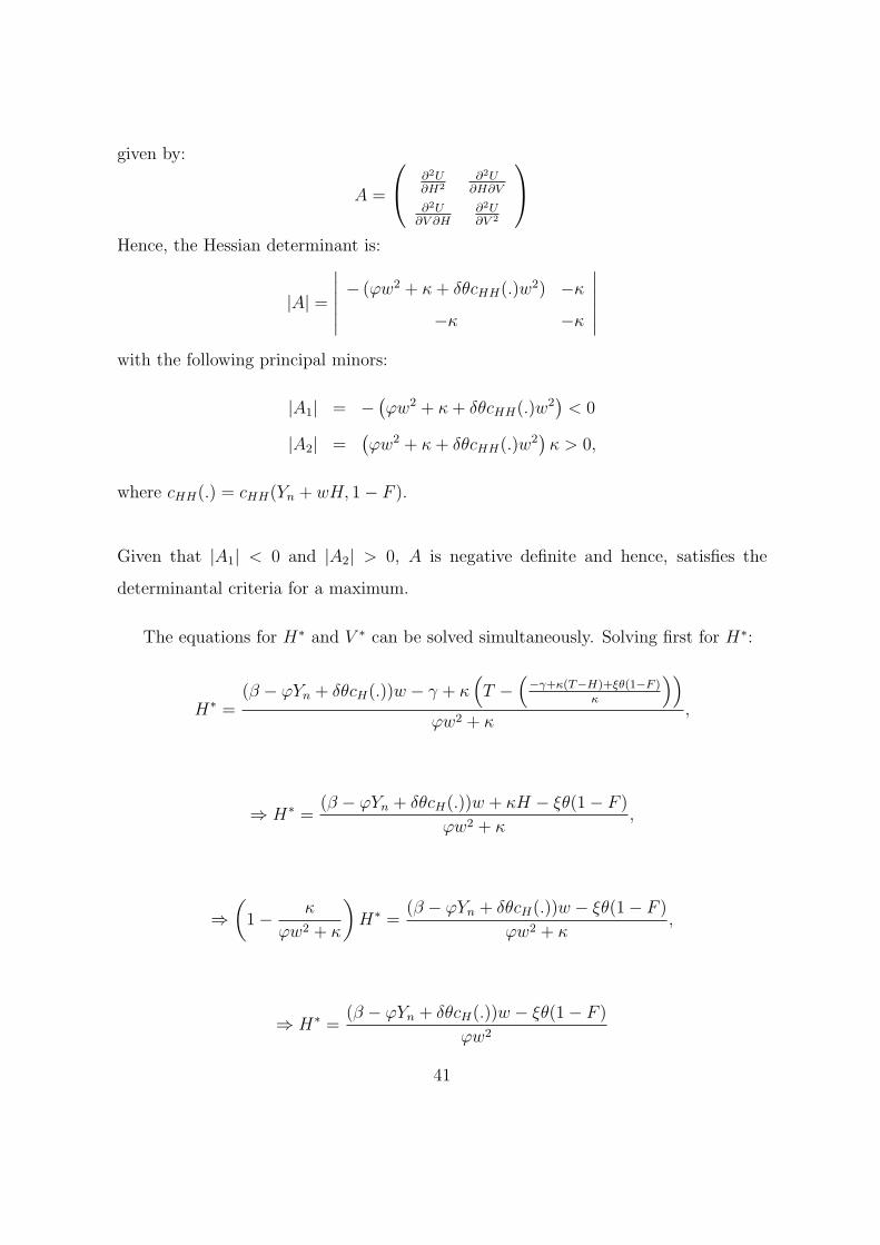
given by:
A =
∂2U∂H2
∂2U∂H∂V
∂2U∂V ∂H
∂2U∂V 2
Hence, the Hessian determinant is:
|A| =
∣∣∣∣∣∣ − (ϕw2 + κ + δθcHH(.)w2) −κ
−κ −κ
∣∣∣∣∣∣with the following principal minors:
|A1| = −(ϕw2 + κ + δθcHH(.)w2
)< 0
|A2| =(ϕw2 + κ + δθcHH(.)w2
)κ > 0,
where cHH(.) = cHH(Yn + wH, 1− F ).
Given that |A1| < 0 and |A2| > 0, A is negative definite and hence, satisfies the
determinantal criteria for a maximum.
The equations for H∗ and V ∗ can be solved simultaneously. Solving first for H∗:
H∗ =(β − ϕYn + δθcH(.))w − γ + κ
(T −
(−γ+κ(T−H)+ξθ(1−F )
κ
))ϕw2 + κ
,
⇒ H∗ =(β − ϕYn + δθcH(.))w + κH − ξθ(1− F )
ϕw2 + κ,
⇒(
1− κ
ϕw2 + κ
)H∗ =
(β − ϕYn + δθcH(.))w − ξθ(1− F )
ϕw2 + κ,
⇒ H∗ =(β − ϕYn + δθcH(.))w − ξθ(1− F )
ϕw2
41
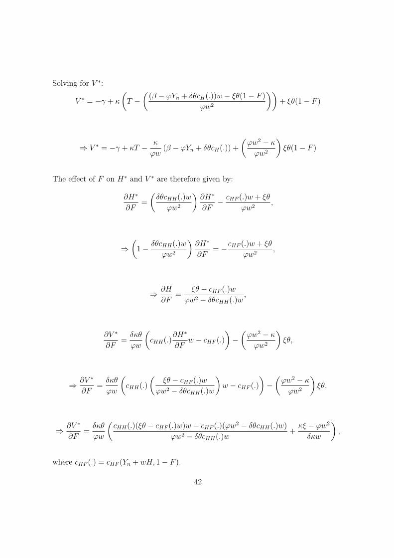
Solving for V ∗:
V ∗ = −γ + κ
(T −
((β − ϕYn + δθcH(.))w − ξθ(1− F )
ϕw2
))+ ξθ(1− F )
⇒ V ∗ = −γ + κT − κ
ϕw(β − ϕYn + δθcH(.)) +
(ϕw2 − κ
ϕw2
)ξθ(1− F )
The effect of F on H∗ and V ∗ are therefore given by:
∂H∗
∂F=
(δθcHH(.)w
ϕw2
)∂H∗
∂F− cHF (.)w + ξθ
ϕw2,
⇒(
1− δθcHH(.)w
ϕw2
)∂H∗
∂F= −cHF (.)w + ξθ
ϕw2,
⇒ ∂H
∂F=
ξθ − cHF (.)w
ϕw2 − δθcHH(.)w,
∂V ∗
∂F=
δκθ
ϕw
(cHH(.)
∂H∗
∂Fw − cHF (.)
)−
(ϕw2 − κ
ϕw2
)ξθ,
⇒ ∂V ∗
∂F=
δκθ
ϕw
(cHH(.)
(ξθ − cHF (.)w
ϕw2 − δθcHH(.)w
)w − cHF (.)
)−
(ϕw2 − κ
ϕw2
)ξθ,
⇒ ∂V ∗
∂F=
δκθ
ϕw
(cHH(.)(ξθ − cHF (.)w)w − cHF (.)(ϕw2 − δθcHH(.)w)
ϕw2 − δθcHH(.)w+
κξ − ϕw2
δκw
),
where cHF (.) = cHF (Yn + wH, 1− F ).
42

7 Appendix B
43
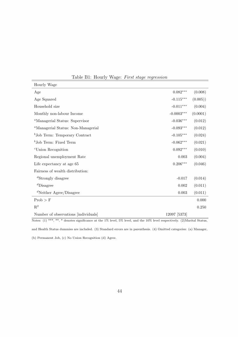
Table B1: Hourly Wage: First stage regression
Hourly Wage
Age 0.082∗∗∗ (0.008)
Age Squared -0.115∗∗∗ (0.005))
Household size -0.011∗∗∗ (0.004)
Monthly non-labour Income -0.0003∗∗∗ (0.0001)aManagerial Status: Supervisor -0.036∗∗∗ (0.012)aManagerial Status: Non-Managerial -0.093∗∗∗ (0.012)bJob Term: Temporary Contract -0.105∗∗∗ (0.024)bJob Term: Fixed Term -0.062∗∗∗ (0.021)cUnion Recognition 0.092∗∗∗ (0.010)
Regional unemployment Rate 0.003 (0.004)
Life expectancy at age 65 0.206∗∗∗ (0.046)
Fairness of wealth distribution:dStrongly disagree -0.017 (0.014)dDisagree 0.002 (0.011)dNeither Agree/Disagree 0.003 (0.011)
Prob > F 0.000
R2 0.250
Number of observations [individuals] 12097 [5373]Notes: (1) ***, **, * denotes significance at the 1% level, 5% level, and the 10% level respectively. (2)Marital Status,
and Health Status dummies are included. (3) Standard errors are in parenthesis. (4) Omitted categories: (a) Manager,
(b) Permanent Job, (c) No Union Recognition (d) Agree.
44
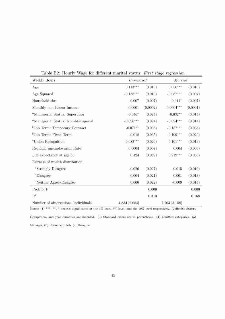
Table B2: Hourly Wage for different marital status: First stage regression
Weekly Hours Unmarried Married
Age 0.113∗∗∗ (0.015) 0.056∗∗∗ (0.010)
Age Squared -0.138∗∗∗ (0.010) -0.087∗∗∗ (0.007)
Household size -0.007 (0.007) 0.011∗ (0.007)
Monthly non-labour Income -0.0001 (0.0002) -0.0004∗∗∗ (0.0001)aManagerial Status: Supervisor -0.046∗ (0.024) -0.032∗∗ (0.014)aManagerial Status: Non-Managerial -0.096∗∗∗ (0.024) -0.094∗∗∗ (0.014)bJob Term: Temporary Contract -0.071∗∗ (0.036) -0.157∗∗∗ (0.038)bJob Term: Fixed Term -0.018 (0.035) -0.109∗∗∗ (0.029)cUnion Recognition 0.083∗∗∗ (0.020) 0.101∗∗∗ (0.013)
Regional unemployment Rate 0.0004 (0.007) 0.004 (0.005)
Life expectancy at age 65 0.124 (0.089) 0.219∗∗∗ (0.056)
Fairness of wealth distribution:dStrongly Disagree -0.026 (0.027) -0.015 (0.016)dDisagree -0.004 (0.021) 0.001 (0.013)dNeither Agree/Disagree 0.006 (0.022) -0.009 (0.014)
Prob > F 0.000 0.000
R2 0.313 0.168
Number of observations [individuals] 4,834 [2,684] 7,263 [3,158]Notes: (1) ***, **, * denotes significance at the 1% level, 5% level, and the 10% level respectively. (2)Health Status,
Occupation, and year dummies are included. (3) Standard errors are in parenthesis. (4) Omitted categories: (a)
Manager, (b) Permanent Job, (c) Disagree.
45
References
[1] Adams, Stacy J., and William B. Rosenbaum (1962), ”The Relationship of Worker
Productivity to Cognitive Dissonance About Wage Inequities”, Journal of Applied
Psychology, 46(3):161–164.
[2] Adams, Stacy J. (1965), ”Inequity in Social Exchange”, Advances in Experimental
Social Psychology, in L. Berkowitz (ed), pp. 267–299, New York: Academic press.
[3] Akerlof, George A. (1980), ”A Theory of Social Custom, of Which Unemployment
May be One Consequence”, The Quarterly Journal of Economics, 94(4):749–775.
[4] Akerlof, George A. (1982), ”Labor Contracts as Partial Gift Exchange”, The Quar-
terly Journal of Economics, 97(4):543–569.
[5] Akerlof, George A., and Janet Yellen (1990), ”The Fair Wage-Effort Hypothesis
and Unemployment”, The Quarterly Journal of Economics, 101(1):83–96.
[6] Amiel, Yoram, John Creedy, and Stan Hurn (1999), ”Measuring Attitudes Towards
Inequality”, Scandinavian Journal of Economics, 105(2):255–283.
[7] Andrews, I.R. (1967), ”Wage Inequity and Job Performance”, Journal of Applied
Psychology, 51(1):39–45.
[8] Ashenfelter, Orley, Richard Layard (1986), Handbook of Labor Economics, Vol 1,
Amsterdam: North Holland.
[9] Becker, Gary S. (1965), ”A Theory of the Allocation of Time”, The Economic
Journal, 75(299):493–517.
[10] Biddle, Jeff E., and Gary A. Zarkin (1989), ” Choice Among Wage-Hours Packages:
An Empirical Investigation of Male labor Supply”, Journal of Labor Economics,
7(4):415–437.
46
[11] Borjas, George J., (1980), ”The Relationship Between Wages and Weekly Hours
of Work: The Role of Division Bias”, Journal of Human Resources, 15(3):409–423.
[12] Bound, John, David A. Jaeger, and Regina M. Baker (1995), ”Problems with
Instrumental Variables Estimation When the Correlation Between the Instruments
and the Endogenous Explanatory Variable is Weak”, Journal of the American
Statistical Association, 90(430):443–450.
[13] Carlsson, Fredrik, Dinky Daruvala, and Olof Johansson-Stenman (2003), ”Are
People Inequality Averse or Just Risk Averse?”, Unpublished.
[14] Conway, Karen Smith, and Thomas J. Kniesner (1994), ”Estimating Labor Supply
with Panel Data”, Economics Letters, 44:27–33.
[15] Corneo, Giacom and Hans Peter Gruner (2002), ”Individual Preferences for Po-
litical Redistribution”, Journal of Public Economics, 83:83–107.
[16] Cornwell, Christopher, Peter Schmidt, and Donald Wyhowski (1992), ”Simulta-
neous Equations and Panel Data”, Journal of Econometrics, 51:151–181.
[17] Cornwell, Christopher, Karen L. Tinsley, and Ronald S. Warren Jr. (2000), ”Re-
ligious Background and the Labor Supply and Wages of Young Women”, Unpub-
lished.
[18] de Neubourg, Chris, and Maarten Vendrik (1994), ”An extended Rationality
Model of Social Norms in Labour Supply”, Journal of Economic Psychology,
15:93–126.
[19] Elster, John (1998), ”Emotions and Economic Theory”, Journal of Economic
Literature, 34:47–74.
[20] Epstein Gil S. and Uriel Spiegel (2001),”Natural Inequality, Production and Eco-
nomic Growth”, Labour Economics, 8:463–473.
47
[21] Fehr, Ernst, Georg Kirchsteiger, and Arno Riedl (1993), ”Does Fairness Prevent
Market Clearing? An Experimental Investigation”, Quarterly Journal of Eco-
nomics, 108(2):437–459.
[22] Fehr, Ernst, and Klaus Schmidt (1999), ”A Theory of Fairness, Competition and
Cooperation”, Quarterly Journal of Economics, 114(3):817–868.
[23] Feldman, Daniel C. (2002), ”Managers’ Propensity to Work Longer Hours – A
multilevel Analysis”, Human Resource Management Review, 12:339–357.
[24] Fong, Christina (2001), ”Social Preferences, Self-interest, and the Demand for
Redistribution”, Journal of Public Economics, 82:225–246.
[25] Fong, Christina, Samuel Bowles, and Herbert Gintis (2002), ”Behavioral Founda-
tions of Egalitarianism, Reciprocity, and Altruism”, Unpublished.
[26] Foster, Michael, and Mark Pearson (2002), ”Income Distribution and Poverty in
the OECD Area: Trends and Driving Forces” OECD Economic Studies, No. 34,
2002/I.
[27] Galor, Oded, and Joseph Zeira (1993), ”Income Distribution and Macroeco-
nomics”, The Review of Economic Studies, 60(1):35–52.
[28] Goodman, Alissa (2001), ”Inequality and Living Standards in Great Britain: Some
Facts”, The Institute for Fiscal Studies, Briefing Note No.19.
[29] Greene, William H. (2000), Econometric Analysis, 4th Edition, New Jersey: Pren-
tice Hall International, Inc.
[30] Gronau, Rueben (1977), ”Leisure, Home Production, and Work – The Theory of
the Allocation of Time Revisted”, The Journal of Political Economy, 85(6):1099–
1124.
48
[31] Gronau, Rueben (1997), ”The Theory of Home Production: The Past Ten Years”,
Journal of Labor Economics, 15(2):197–205.
[32] Hausman, Jerry A. (1978),”Specification Tests in Econometrics”, Econometrica,
46:1251-1271.
[33] Hausman, Jerry A. (1983), ”Specification and Estimation of Simultaneous Equa-
tion Models”, Handbook of Econometrics, pg 391–448, Z. Griliches and M.D. In-
triligator (ed), Volume 1 Amsterdam: North Holland.
[34] Heckman, James (1993), ”What Has Been Learned About Labor Supply in the
Past Twenty Years”, The American Economic Review, 83(2):116–121.
[35] Kahneman, Daniel, Jack Knetsch, and Richard Thaler (1986a), ”Fairness as a
Constraint on Profit Seeking: Entitlements in the Market”, The American Eco-
nomic Review, 76(4):728–741.
[36] Kahneman, Daniel, Jack Knetsch, and Richard Thaler (1986b), ”Journal of Busi-
ness”, The American Economic Review, 59(4):S285–S300.
[37] Kelly, Morgan (2000), ”Inequality and Crime”, The Review of Economics and
Statistics, 82(4):530–539.
[38] Korzeniewicz, Roberto Patricio, and Timothy Patrick Moran (1997), ”World-
Economic Trends in the Distribution of Income”, American Journal of Sociology,
102(4):1000–1039.
[39] Lee, Woojin and John E. Roemer (1998), ”Income Distribution, Redistributive
Politics, and Economic Growth”, Journal of Economic Growth, 3:217–240.
[40] Levine, David I. (1992), ”Piece Rates, Output Restriction, and Conformism”,
Journal of Economic Psychology, 13:473–489.
49
[41] Milanovic, Brian (2002), ”True World Income Distribution, 1988 and 1993: First
Calculation Based on Household Surveys Alone”, The Economic Journal, 112:51–
92.
[42] Mundlak, Yair (1978), ”On The Pooling of Time Series and Cross Section Data”,
Econometrica, 46(1):69–85.
[43] Pencavel, John (1986), ”Labour Supply of Men: A Survey”, In Handbook of Labour
Economics, (ed. O. Ashenfelter and R. Layard), Amsterdam: North-Holland.
[44] Persson, Torsten, and Guido Tabellini (1994), ”Is Inequality Harmful for Growth”,
The American Economic Review, 84(3):600–621.
[45] Romer, David (1984), ”The Theory of Social Custom: A Modification and Some
Extensions”, The Quarterly Journal of Economics, 99(4):717–727.
[46] Roy, Kakoli, and Susanne Ziemek (2000), ”On The Economic of Volunteering”,
ZEF Discussion Papers on Development Policy, No. 31.
[47] Rutstrom, Elisabet E. and Melonie B. Williams (2000), ”Entitlements and fair-
ness: An Experimental Study of Distributive Preferences”, Journal of Economic
Behavior and Organization, 43:75–89.
[48] Sala-i-Martin, Xavier (2002), ”The World Distribution of Income (Estimated From
Individual Country Distributions)”, unpublished.
[49] Staiger, Douglas, and James H. Stock (1997), ”Instrumental Variables Regression
with Weak Instruments”, Econometrica, 65(3):557–586.
[50] Stutzer, Alois, and Rafael Lalive (2001), ”The Role of Social Work Norms in Job
Searching and Subjective well-Being”, IZA Discussion Paper, No. 300.
[51] Taylor, M.F (ed. with J. Brice et al) (1996), British Household Panel Survey User
Manual Volumes A and B, University of Essex, Colchester.
50
[52] Thaler, Richard H. (1985), ”Mental Accounting and Consumer Choice”, Marketing
Science, 4(3):199–214.
[53] Thurow, Lester (1971), ”The Income Distribution as a Pure Public Good”, The
Quarterly Journal of Economics, 85(2):327–336.
[54] Vella, Francis, (1998), ”Estimating Models With Sample Selection Bias: A Sur-
vey”, Journal of Human Resources, 33(1):127–169.
[55] Wooldridge, Jeffrey M. (2002), Econometric Analysis of Cross Section and Panel
Data, United States: MIT.
51