Does the growth of structure affect our dynamical models of the Universe? The averaging,

backreaction, and fitting problems in cosmology

This article has been downloaded from IOPscience. Please scroll down to see the full text article.

2011 Rep. Prog. Phys. 74 112901

(http://iopscience.iop.org/0034-4885/74/11/112901)

Download details:

IP Address: 129.25.131.235

The article was downloaded on 17/03/2013 at 09:10

Please note that terms and conditions apply.

View the table of contents for this issue, or go to the journal homepage for more

Home Search Collections Journals About Contact us My IOPscience

IOP PUBLISHING REPORTS ON PROGRESS IN PHYSICS

Rep. Prog. Phys. 74 (2011) 112901 (17pp) doi:10.1088/0034-4885/74/11/112901

Does the growth of structure affect ourdynamical models of the Universe?The averaging, backreaction, and fittingproblems in cosmologyChris Clarkson1, George Ellis1, Julien Larena1,2 and Obinna Umeh1

1 Astrophysics, Cosmology and Gravity Centre, and Department of Mathematics and Applied Mathematics,University of Cape Town, Rondebosch 7701, South Africa2 Department of Mathematics, Rhodes University, 6140 Grahamstown, South Africa

Received 24 February 2011, in final form 29 July 2011Published 27 October 2011Online at stacks.iop.org/RoPP/74/112901

AbstractStructure occurs over a vast range of scales in the Universe. Our large-scale cosmological modelsare coarse-grained representations of what exists, which have much less structure than there reallyis. An important problem for cosmology is determining the influence the small-scale structure inthe Universe has on its large-scale dynamics and observations. Is there a significant, generalrelativistic, backreaction effect from averaging over structure? One issue is whether the process ofsmoothing over structure can contribute to an acceleration term and so alter the apparent value ofthe cosmological constant. If this is not the case, are there other aspects of concordance cosmologythat are affected by backreaction effects? Despite much progress, this ‘averaging problem’ is stillunanswered, but it cannot be ignored in an era of precision cosmology, for instance it may affectaspects of baryon acoustic oscillation observations.

(Some figures in this article are in colour only in the electronic version)

This article was invited by F Bernardeau.

Contents

1. Introduction 12. Averaging, backreaction and fitting 2

2.1. The lumpy Universe and the background 22.2. Averaging and backreaction 32.3. Fitting and observations 4

3. Non-perturbative backreaction 53.1. Averaging formalisms 53.2. Other approaches 63.3. Model building approaches 7

4. Perturbative backreaction 84.1. Backreaction in the standard model 8

4.2. Short wavelength approximation 124.3. Effective fluid approach 124.4. Discussion 13

5. The alternatives 145.1. The skeptic 145.2. The enthusiast 145.3. The fence-sitter 145.4. Open issues and future directions 14

6. Conclusion 15Acknowledgments 15References 15

1. Introduction

A crucial feature of the real Universe is that structure occurson many scales. Large-scale models of the Universe, such

as the standard models of cosmology, are coarse-grainedrepresentations of what is actually there, which has much morestructure than is represented by those models. An importantissue for cosmology is the question of whether the smaller scale

0034-4885/11/112901+17$88.00 1 © 2011 IOP Publishing Ltd Printed in the UK & the USA

Rep. Prog. Phys. 74 (2011) 112901 C Clarkson et al

structures influence the dynamics of the Universe on largerscales: is there a significant backreaction effect from the smallscales to the large scales?

The standard Friedmann–Lemaıtre–Robertson–Walker(FLRW) models of cosmology are a resounding success.They can account for all observations to date with just ahandful of parameters. These are the simplest reasonablyrealistic Universe models possible within general relativity:homogeneous, isotropic, and flat to a first approximation,with a scale-invariant spectrum of Gaussian perturbations frominflation added on top to account for structures down to thescale of clusters of galaxies. Only the physical motivationfor the value of the cosmological constant and the associatedcoincidence problem is required for a complete understandingat late times. Cosmology in the future will be refining thispicture.

But is it as simple as this? The Universe may wellbe statistically homogeneous and isotropic above a certainscale, but on smaller scales it is highly inhomogeneous, quiteunlike an FLRW Universe. General relativity is a theoryin which spacetime itself is the dynamical field with noexternal reference space. Yet it is ubiquitous in cosmologyto talk of a ‘background’ which is exactly homogeneousand isotropic, on which galaxies and structure exist asperturbations. Is this the same as starting with a more detailedtruly inhomogeneous metric of spacetime, and progressivelysmoothing it—probably by a non-covariant process—until weget to this background?

It is commonly assumed that whichever way one goesabout it the results of these two processes must be the same;but the non-linearity of the field equations ensures that they arenot. The problem for cosmologists is whether this differenceis important. This has been the subject of controversy, withopinions ranging from the suggestion it could completelyexplain the recently observed accelerating expansion of theUniverse without a need for any dark energy [1–7] to the claimthat it is completely negligible [8–19], with a middle-ground ofpapers claiming it is enough to disturb the cosmic concordanceof the standard model [20–28].

Averaging has kinematic, dynamical and observationalaspects. One estimate of the importance of this effect wouldbe to note that within the standard model, variations in theexpansion rate of around a few per cent occur on scales oforder 100 Mpc [20, 22, 23, 25, 28–31]. At the very least, then,the averaging problem may be important for observations inprecision cosmology; indeed it is obviously built into standardobservational practice.

But does it have dynamic consequences? Green and Wald[19] claim to derive in a rigorous and systematic way the effectsof small-scale inhomogeneities on large-scale dynamics, andthereby prove that matter inhomogeneities produce no neweffects on the dynamics of the background metric: they canonly mimic radiation. However, others reach an oppositeconclusion: Buchert’s approach [1, 2] shows backreactionfrom inhomogeneity can potentially mimic dark energy;Kolb and colleagues concur [32], and even have suggestedinhomogeneity effects can fully explain the acceleration ofthe Universe [5, 33], as has Wiltshire [34, 35]. Recently

Baumann et al [18], using second-order perturbation theory,have claimed that virialized structures freeze out of the cosmicexpansion and only affect the background dynamics througha renormalized mass. Clearly there is no agreement, buteven from a conservative viewpoint there is evidence thatbackreaction might have an impact on precision cosmology:Baumann et al [18] conclude that inter alia it significantlyaffects the baryon acoustic oscillations (BAO).

This review. Our aim in this paper is to present the differentapproaches to the dynamical aspects of backreaction effectsin recent eras in cosmology, highlighting open questions andfuture research agendas. While we will briefly touch on them,we will not deal comprehensively with observational aspectsof the fitting problem: this raises a number of further issues wedo not have space to deal with here [36]. We will also not dealwith possible backreaction effects in the very early Universe,which raise a rather different set of issues (see, e.g., [37, 38]).

There have been quite a number of attempts to estimatethe backreaction effect. One set is based on starting withan inhomogeneous model and using some averaging processto produce an approximately FLRW model. This has beendeveloped both in terms of general formalisms, and in termsof detailed model building. Alternatively, by averaging overstructure in the standard model, the backreaction effect canbe calculated perturbatively; this should then provide anestimate of its size, and, in principle, allows us to evaluatethe fluctuations which become of the order of the mean, andthe background one starts with no longer correctly describesthe averages.

We first discuss non-perturbative attempts to estimatebackreaction. Then we provide an overview of backreaction inthe standard model, where it appears that the effect is small—atleast to second order in perturbation theory—but neverthelessis at least sufficient to affect precision cosmology results.

2. Averaging, backreaction and fitting

2.1. The lumpy Universe and the background

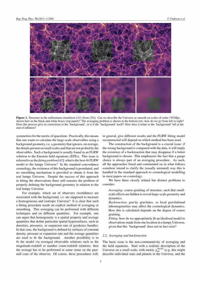
Any description of physical reality embodies a scale ofaveraging that is usually not made explicit. The world lookscompletely different depending on the scale of descriptionchosen; for example, a fluid looks wholly different on aneveryday scale (say 1 m) as opposed to atomic scale (say10−11 m). The same is true for astronomy and cosmology.The background models in standard cosmology are the FLRWmodels, which ignore all local structural details. More realisticmodels include linearized perturbations about this background,in principle representing the largest scale growing structuresdown to the scale of clusters of galaxies (tens of Mpc) fromearly times to today; but they do not represent the non-linearsmaller scale structures, such as our galaxy or the solar system,at later times. The Universe looks far from homogeneous whenviewed on any scale from 1 AU to 1 Mpc, and only approachesstatistical homogeneity past 100 Mpc (though even this is indispute [39, 40])—see figure 1.

To describe the Universe on its largest scales, one has tomake approximations that postulate or derive a high degree of

2

Rep. Prog. Phys. 74 (2011) 112901 C Clarkson et al

Figure 1. Structure in the millennium simulation [41] (from [26]). Can we describe the Universe as smooth on scales of order 150 Mpc,shown here in the black and white boxes (top panel)? The averaging problem is shown in the bottom row: how do we go from left to right?Does this process give us corrections to the ‘background’, or is it the ‘background’ itself? How does it relate to the ‘background’ left at theend of inflation?

symmetries for the metric of spacetime. Practically, this meansthat one wants to calculate the large-scale observables using abackground geometry, i.e. a geometry that ignores, on average,the details present on small scales and that are not probed by theobservables. Such a background is usually found in an FLRWsolution to the Einstein field equations (EFEs). This issue isreferred to as the fitting problem [42]: what is the best-fit FLRWmodel to the lumpy Universe? In the standard concordancecosmology, the existence of this background is postulated, andno smoothing mechanism is provided to obtain it from thereal lumpy Universe. Despite the success of this approachin fitting the observations there still remains the problem ofproperly defining the background geometry in relation to thereal lumpy Universe.

For example, which set of observers (worldlines) areassociated with the background, i.e. are supposed to measurea homogeneous and isotropic Universe? It is clear that sucha fitting procedure needs an explicit method of averaging orsmoothing. This averaging can be performed with differenttechniques and on different quantities. For example, onecan argue that homogeneity is a spatial property and averagequantities that define particular spatial hypersurfaces, such asdensities, pressures, or expansion rate of geodesics bundles.In that case, the background is defined by surfaces of constantdensity, pressure or expansion rate and the average quantitiesare used to fit the background. Another possibility is tofit the model via averaged observable relations such as themagnitude-redshift or number count-redshift relations; thenthe average has to be performed in some sense on the past-null cone of the observer. Of course, these procedures will,

in general, give different results and the FLRW fitting modelreconstructed will depend on which method has been used.

The construction of the background is a crucial issue: ifthe wrong background is compared with the data, it will implythe existence of a backreaction that may disappear if a betterbackground is chosen. This emphasizes the fact that a gaugechoice is always part of an averaging procedure. As such,all the approaches listed and commented on in what followssomehow intend to clarify the (usually unstated) way this ishandled in the standard approach to cosmological modellingin most papers on cosmology.

We have three closely related but distinct problems toconsider:

Averaging: coarse-graining of structure, such that small-scale effects are hidden to reveal large-scale geometry anddynamics.Backreaction: gravity gravitates, so local gravitationalinhomogeneities may affect the cosmological dynamics.How this is calculated depends on the degree of coarsegraining.Fitting: how do we appropriately fit an idealized model toobservations made from one location in a lumpy Universe,given that this ‘background’ does not in fact exist?

2.2. Averaging and backreaction

The basic issue is the non-commutativity of averaging andthe field equations. Start with a realistic description of theUniverse on a small scale, with metric g

(local)ab (e.g. this might

describe individual stars and planets in the Universe, and the

3

Rep. Prog. Phys. 74 (2011) 112901 C Clarkson et al

vacuum between them). Average it by a smoothing procedureto a metric g

(gal)ab with an averaging scale where galaxies are

well represented but individual stars are invisible. Average thisin turn to a metric g

(lss)ab with an averaging scale where large-

scale structures are well represented but individual galaxiesare invisible (there are many possible scales that are omittedin this description). The largest scale (completely smoothed)model will have an FLRW metric g

(cos)ab , where all traces of

inhomogeneity have been removed. There will similarly beaveraged stress energy tensors T

(local)ab , T

(gal)ab , T

(lss)ab , T

(cos)ab

representing the matter present at each of these scales.Now the Einstein equations may be assumed to hold at the

‘local’ scale: after all, this is the scale where they have beenexquisitely checked, so

R(local)ab − 1

2R(local)g(local)ab + �g

(local)ab = κT

(local)ab . (1)

But the averaging process,

g(local)ab → g

(gal)ab → g

(lss)ab , T

(local)ab → T

(gal)ab → T

(lss)ab ,

(2)

does not commute with evaluating the inverse metric,connection coefficients, Ricci tensor and Ricci scalar, forexample

g(local)ab → g(local)ab → �(local)c

ab → R(local)ab → R(local), (3)

g(gal)ab → g(gal)ab → �(gal)c

ab → R(gal)ab → R(gal). (4)

Hence if the EFEs hold at ‘local’ scale (i.e. equation (1) istrue), they will not hold at scales ‘gal’ or ‘lss’; for example,one will find

R(gal)ab − 1

2R(gal)g(gal)ab + �g

(gal)ab = κT

(gal)ab + E

(gal)ab , (5)

where the extra term E(gal)ab �= 0 is due to this non-

commutativity. It is the effective matter source termrepresenting the effect of averaging out smaller scalestructures, which is then an effective source term for averagedEFE at scale ‘gal’. Similarly there will be such an effectivesource term E

(lss)ab at that scale—the scale usually represented

by perturbed FLRW models—and E(cos)ab at the cosmological

scale. This is the backreaction from the small scales to thelarger scales.

In essence, it is an assumption that Einstein’s equationsalso hold for an averaged geometry, as well as a local one. Infact, it is not clear that the whole machinery of general relativityholds after averaging—e.g. concepts such as spacetime andobjects such as tensors need to be assumed to make sense aftercoarse graining.

The classic example of this effect is Isaacson’s calculationof the effective backreaction of small-scale gravitationalradiation on an averaged large-scale metric [43, 44]. Now thisaffect applies to cosmology: if there is significant gravitationalradiation at early times, this will affect the dynamics at latertimes, according to Isaacson’s calculation (which can alsobe derived from a variational principle, see [45]). However,that effect will be exceedingly small at late times (it may besignificant at early times, see [37, 38]).

We are concerned, however, with the dynamic effectsof non-linear structure on cosmology at late times (i.e. after

decoupling of matter and radiation). In principle, the sameeffect will occur in this context [46]; the question is whetherthis is a significant effect or not. We will look at generalformalisms and specific models in the next section.

2.3. Fitting and observations

One can do a spacetime fitting, asking which FLRW model isbest if we average invariant quantities in a spatial or spacetimevolume: e.g. the energy density of particles and their velocities(when the matter averaging may be represented by kinetictheory); one may choose to smooth the metric or scalarinvariants on the geometry side. Alternatively, one can do a nullfitting, where one in effect averages astronomical observations.

2.3.1. Fitting and the past-null cone. As we determineour best-fit model by null cone observations, this is inthe end what we would like to do (in effect the standardobservational cosmology approach is this type, but is notusually phrased this way). So a key issue is how this allrelates to cosmological observations. Here we have to takeinto account not only the effect of averaging on the geometryand dynamics (as represented by (5)) but also the effect oflumps on null geodesics and on observational relations.

The basic question is: What are observables in theseapproaches? What do observations of averaged quantitiesreally tell us about our Universe? Cosmological observationsprobe quantities such as the redshift, the angular-diameterdistance, the luminosity distance, and the image distortion,i.e. quantities related to light emitted by a distance source andpropagating on the past-null cone. The general way this workswas described in a perturbative framework in the pioneeringwork of Kristian and Sachs [47] (extended to more generalcases in [48–50]). This involves expanding the geodesicdeviation vector in orders of the affine parameter along thepast-null cone. Here one relates the geometric quantities tothe observational quantities using the relation between theredshift and the four-velocity of the observer ua: 1+z = uak

a |eubkb|o ,

and the relation between the intrinsic cross-sectional area dA

of a distant source and the measured solid angle subtendedby the observer d�: dA = r2

A d�, where r2A is the angular-

diameter distance. This expansion as given by [48, 49] isexactly covariant and can be applied to any spacetime. In thepresent context one would like to compare the general resultwith that of the FLRW background. This is done by matchingthe background FLRW results with that from the spacetimeindicated by observations [9, 51].

However, there are complications. In the real Universe,as pointed out in [47, 49, 52, 53], observations take place vianull geodesics lying in the empty spacetime between galaxies,which are focused only by the curvature actually inside thebeam, not the matter that would be there in a completelyuniform model. The effect on the observational relationsof introducing inhomogeneities into a given backgroundspacetime is twofold: it alters the redshift, and it changes areadistances. This should also be taken into account in any fittingprocedure.

4

Rep. Prog. Phys. 74 (2011) 112901 C Clarkson et al

Others have emphasized the importance of smoothing thepast lightcone. A sketch of how the averaged Raychauhduriequation on the past-null cone would look like was givenin [54], while Rasanen in [55, 56] gave the past-nullcone averaged equations for the scalars in a statisticallyhomogeneous and isotropic spacetime. Work in this importantarea is still at its infant stage with no concrete quantifiablephysical result that can be directly fitted to observations.

2.3.2. Averaging on the past light cone. Averaging is in somerespects a fitting process, but does not necessarily correspondto any actual observational procedure. Can one propose anaverage model of the Universe based on the past-null cone? Avery recent attempt at a comprehensive approach was made byGasperini et al [57]. However, this should be approached withcaution: observations to cosmological distances mix spatialand time variation, and it does not make sense to simplyaverage today’s state of the Universe with what it was likein the past. One would expect any averaging operation toleave the background invariant, and it is not obvious that thiscan happen for FLRW somehow averaged on its light cones.So averaging based on observations would need to involvecomparing the Universe today with earlier times by the use ofdynamical equations relating variables at these different times:a very model dependent procedure, and not ‘averaging’ in anormal sense.

What is clear is that backreaction will not be importantalong the light cone, because the key causal effects incosmology propagate in a timelike fashion [58]. Neverthelessit is obviously important to relate the results of averagingand backreaction effects to observations. The exact andperturbation approaches that follow attempt to do this.

3. Non-perturbative backreaction

One approach is to build a model of the Universe ‘bottomup’. Advocated by Buchert [1, 2, 59], Zalaletdinov [60, 61],Wiltshire [34, 35, 62], Rasanen [6, 55, 56], among others[63–67], these approaches dispute the idea that one needs abackground to work from: rather the background model andits dynamics should emerge as a large-scale approximation to amore detailed inhomogeneous model, which can be comparedwith an FLRW model for the Universe assumed ab initio asin the standard approach. As explained in previous sections,the field equations for such a model may be expected to bedifferent from those in a standard FLRW model: we want tounderstand that difference.

Non-perturbative approaches fall into two main cate-gories. One are generic averaging formalisms, which aim tounderstand the nature of the backreaction terms in general, abit like deriving and understanding the macroscopic Maxwellequations. The other approach is to create fully relativisticinhomogeneous or even N -body models by the use of simpli-fying assumptions; then, by comparing observables in thesemodels with their averaged FLRW counterparts one can hopeto quantify non-perturbatively the backreaction effect and themagnitude of the fitting problem. Let us consider each ap-proach in turn, with some of the main attempts in the literature.

3.1. Averaging formalisms

3.1.1. Buchert’s approach. Alongside early attempts[20, 68–71], Buchert [1, 2] builds on the Newtonian averagingby Buchert and Ehlers [72, 73] to provide a bare-bonesapproach to the problem, concentrating on averaging scalarson spatial hypersurfaces. The kinematic scalar equations forvorticity-free perfect fluid are averaged, to give evolutionequations for the averaged expansion and shear scalars.Several authors [2, 14, 25, 55, 74, 75] have generalized thisapproach to any arbitrary spacetime, but we will illustrate theapproach with the original Buchert proposal.

Let us assume a dust spacetime, and observers andcoordinates at rest with respect to the dust. The average ofa scalar quantity S may be (non-covariantly) defined as simplyits integral over a region of a spatial hypersurface D of constantproper time divided by the Riemannian volume:

〈S(t, x)〉D = 1

VD

∫D

√det h d3x S(t, x). (6)

Taking the time derivative of equation (6) yields thecommutation relation

[∂t ·, 〈·〉D]S = 〈�S〉D − 〈�〉D〈S〉D, (7)

where � is the expansion of the dust, and we assume thedomain is comoving with the dust. The dimensionless volumescale factor is defined as aD ∝ VD

1/3, which ensures 〈�〉D =3∂t ln aD . Then, the second derivative of the scale factor isgiven by the averaged Raychaudhuri equation:

3aD

aD+ 4πG〈ρ〉D = � + QD, (8)

where QD = 23 [〈�2〉D − 〈�〉2

D] − 2〈σ 2〉D is the kinematicbackreaction term and σ 2 = 1

2σabσab is the magnitude of the

shear tensor. The non-local variance of the local expansionrate can act in the same way as the cosmological constant,causing the average expansion rate to speed up, even if the localexpansion rate is slowing down. Even more tantalizingly, if thiswere the cause of the observed acceleration, the coincidenceproblem would be solved in the most natural way: as structureforms the variance in the expansion rate grows, as mattercoalesces and virializes [3]. This is a truly remarkablepossibility in moving from local to non-local quantities on anon-trivial geometry, and is the reason for the recent excitementin the averaging problem.

One can see how this counter-intuitive idea works asfollows [76]: if the average scale factor of a universal domain,aD, can be written as a union of locally homogeneous andisotropic regions, each with its scale factor ai , then theacceleration of the universal domain D is given by [6, 77, 78]

a2DaD = a2

1 a1 + a22 a2

+ · · · +2

a3D

∑i �=j

a3i a

3j

(ai

ai

− aj

aj

)2

, (9)

where ai represents the locally defined scale factor in the ithsub-region, and, aD ≡ (a3

1 + a32 + · · ·)1/3. Acceleration of the

5

Rep. Prog. Phys. 74 (2011) 112901 C Clarkson et al

universal domain, aD > 0, can easily be achieved, for example,for a two disjointed dust filled FLRW sub-region in which onemight be expanding while the other is contracting at a time t ,i.e. a1 = −a2 (assuming same sized sub-regions a ≡ a1 = a2),one obtains a2

DaD = 2a3{ aa

+ 4( aa)2} = 7

3κ2a3ρ > 0. Hereone easily obtains an acceleration for the universal domain,aD > 0, even when the two sub-regions are deceleratinga1 < 0, a2 < 0; i.e. all observers see only deceleration.However, it has been argued [8] that acceleration found in thistoy model does not necessary imply that the physical Universeis accelerating, since this model has not been shown to satisfyother rigorous observational tests. It also ignores problemsdue to matching/junction conditions for any two regions.

In Buchert’s scheme, all tensor contributions appear asscalars in these equations, and are collected into unknownsource terms. Of course, the system of scalar equations isnot closed, so one has to make an ansatz about the effect ofaveraging the shear terms; so it is very difficult to say how bigthe backreaction effect is. One can derive an evolution equationfor the averaged shear scalar; but that would be sourced byproducts of Weyl curvature tensors, amongst other things, andone quickly sees that the system of equations can never close.So the method of averaging only scalars reaches this limitationquickly. This feature can further be understood by consideringthe integrability condition:

1

a6D

∂t (QDa6D) +

1

a2D

∂t (〈R〉Da2D) = 0 (10)

where 〈R〉D is the average local curvature. This couplingbetween the curvature and the volume scale factor impliesthat if 〈R〉D ∼ a−2

D as in FLRW cosmology, the kinematicbackreaction term will scale as QD ∼ a−6

D , which mimics thebehaviour of some kind of dark fluid.

Having said that, the author of [79] suggested that,if the scalar curvature invariants can uniquely characterizeany spacetime, a scalar averaging scheme can work ingeneral by averaging these invariants. He thus arrives ata complete, closed way of averaging spacetime using onlyscalars. Whether it is practical remains to be seen.

The averaged quantities in Buchert’s formalism do nothave a clear observational meaning. Nevertheless, it is worthnoting that Rasanen [55, 56] argues that in a statisticallyhomogeneous and isotropic Universe, these average quantitiesare exactly the ones that describe observations along the pastlightcone. It will be interesting to see if such an argument canbe made rigorous.

3.1.2. Zalaletdinov’s macroscopic gravity. A comprehensiveapproach to covariantly averaging tensors was initiated andexplored by Zalaletdinov [60, 61, 80–82] and later by others[66, 67, 83, 84]. It is a foundational attempt to averagethe complete set of Cartan structure equations, in order todefine EFEs for the averaged quantities. This approachis directly inspired by the way in which a macroscopictheory of electromagnetism can be obtained from themicroscopic Lorentz–Maxwell theory [61]. Once averaged,the ‘macroscopic field equations’ resemble Einstein’s, but

with a source term—analogously to the polarization term inmacroscopic Maxwell equations [85].

The core issue of averaging tensors covariantly is managedusing bi-local extensions of tensors, so that they transformas tensors at some point of interest, x, but as scalars in aneighbourhood of the point. Because of that, they can beaveraged over that region . The covariant spacetime averageis defined as [60]

Tab(x) =

∫

Aa′a (x, x ′)Ab′

b (x, x ′)Ta′b′(x ′)√

−g(x ′) d4x ′

∫

√−g(x ′) d4x ′ ,

(11)

where Aa′a (x, x ′) is the bi-local transport operator. The

backreaction generated by the smoothing procedure takes theform of a correlation tensor for the gravitational degrees offreedom which appears as an effective source in the EFEs.Alternatives to this definition, and the resulting averagingscheme were initiated in [67].

Implementing this operation results in a completelycovariant smoothing procedure provided the transportoperators satisfy certain conditions. The result is formallyindependent of the averaging scale and as such can be seen asgenerating a universal description of the collective behaviourof local gravitational degrees of freedom when only theirvery large-scale properties matter (much the same way asthermodynamics encompasses the collective behaviour ofparticles on very large scales compared with the particlesthemselves).

This approach makes an extensive use of transport oftensorial quantities along geodesics, but using the naturalparallel transport bitensor the metric is invariant so that nosmoothed metric is obtained. Hence, it relies on a specificchoice of bitensor that satisfies a set of differential equationsand conditions, in order to imply the correct properties of theaverage. This bitensor is used to evaluate integrals on finitedomains, and it is not clear how the formalism is affected by thechoice of this bitensor [66]. Additionally the averaged Einsteinequations rely on some ‘splitting rules’ (see equations (45)and (48) of [80]) which can be questioned (although they areconsistent with an analysis of high frequency gravitationalwaves, see equation (68) of the same paper).

In [83, 86–88] it is shown that in a flat FLRW macroscopicbackground, the correlation tensor is of the form of a spatialcurvature, while [89] showed that Zalaletdinov’s macroscopicgravity reduces to Buchert’s equations with corrections in anappropriate limit. It has further been employed to evaluatethe backreaction effect in a perturbed FLRW model [90, 91],but the requirement that an FLRW background exists makesthis attempt fall under the category described in section 4.1.While the amplitude of backreaction is similar to that obtainedby simpler means, the details of using such a covariantapproach will be important for an effective fluid descriptionof perturbations at second order, such as in [18].

3.2. Other approaches

Another rigorous approach is based on the deformation of thespatial metric of initial data sets along its Ricci flow [92, 93].

6

Rep. Prog. Phys. 74 (2011) 112901 C Clarkson et al

In principle, this method is a nice, natural way of smoothinga spacetime that can be linked to the standard renormalizationgroup approach of effective field theories [68], but the non-linearity of the Ricci flow equations is a serious complicationthat can lead to the development of singularities along theflow; that makes its use in a cosmological context particularlydifficult. A renormalization group approach to coarse grainingin the very early Universe is given in [38]. A promisingmethod to covariantly coarse-grain inhomogeneous dust flowwas presented in [94] as an extension of Buchert’s approach toinclude tensorial quantities.

3.3. Model building approaches

3.3.1. Timescape cosmology. Another very originalviewpoint called the timescape cosmology has been proposedand investigated by Wiltshire [34, 35, 95]. It is a brave butcontentious attempt to seriously look at the status of boundregions and their interaction with an expanding cosmologicalmodel.

The idea is to separate the Universe into expanding,underdense regions whose boundaries are overdense regionsenclosing virialized regions such as the one we, as observers,live in. An average is then performed spatially (using Buchert’sformalism [59]) to define a reference cosmic background.Interestingly, the amount of backreaction in these modelsis at most of order a few per cent (when normalized as afraction of the energy density) and is not solely responsible forexplaining the apparent cosmic acceleration: the non-standardeffects principally come from the desynchronization of localclocks (in the virialized regions) with respect to cosmic clocksdefined via the average background. Indeed, the gravitationalredshift effects imply different ticking rates for clocks insidethe voids and in the virialized regions. Wiltshire argues thatthe effect is cumulative when an average is performed to definethe background clocks. A possible interpretation of the modelis that the extra redshift effects change the observable relationin the effective FLRW background. As such, the model isnot actually accelerating, but the extra redshift accounts fullyfor the dimming of supernovae because they appear to be ata higher redshift than expected. A detailed discussion of theobservational consequences of the timescape cosmology canbe found in [96, 97].

Wiltshire’s proposal is more original than simply viewingthe problem as one of backreaction of structures on the overallglobal dynamics. It also recognizes that the position of theobserver (in virialized structures as opposed to voids) may beimportant to the fitting problem when the variance in localgeometries becomes large. Nevertheless, it suffers from itsown problems, among which one is the use of a pure two-zones model to describe the Universe, without proper junctionconditions between the zones (this problem is emphasizedin [98, 99]).

3.3.2. Swiss-cheese models. The Swiss-cheese modelconsists of one or more spherically symmetric vacuum regions,each described by a Schwarzchild metric, joined acrossspherical boundaries to an FLRW model [100–104]. This

set-up represents a very natural way to model the part of theUniverse that we see, for example the boundary of a galaxyand intergalactic space, the lack of effect of the expansion ofthe Universe on the motion of planets, etc.

The Swiss-cheese type construction can be adoptedto study the effect of inhomogeneities on cosmologicalobservations in a fully non-linear and relativistic manner. Thealgorithm commonly in use is to start with FLRW metric andcut out comoving holes and fill them with a Schwarzschildmetric, while making sure through the matching conditionsthat the mass in the holes equals the mass that was removed.Hence, Swiss-cheese models do not affect the global dynamicsof a lumpy Universe, i.e there is no dynamical backreactioneffect.

Another more interesting construction is to modify thehomogeneous FLRW metric by the introduction of sphericalregions of the spherically symmetric Lemaıtre–Tolman–Bondi(LTB) dust spacetime [105–113]; a quasi-spherical Szekeresmodel can also be introduced [114]. One has to ensurethrough the matching conditions that the spherical regionof inhomogeneities is comoving and mass compensating, toensure that the LTB and FLRW regions evolve independently.Thus again there are no dynamical backreaction effects.

There are, however, significant observational differencesfrom standard cosmology. These spacetimes model preciselythe difference between Weyl and Ricci focussing of nullgeodesics. The null geodesics in the void regions are focussedonly by shear induced by the Weyl tensor. One of the criticalproblems in this area is the relation between Ricci curvature andWeyl curvature, and Swiss-cheese models are a very interestingway to study this. We refer to other papers for a discussionof these observational effects; see [105–111, 113] for differingviewpoints.

3.3.3. Lindquist–Wheeler type models. All the precedingmodels relied on the hypothesis that a cosmological fluidcan be employed to model the distribution of matter in theUniverse. In contrast, Lindquist–Wheeler type models area genuine approach at constructing an expanding Universemodel out of locally static domains. It consists in modelling theUniverse by approximately paving its compact spatial sections3

(topologically homomorphic to S3) with Schwarzchilddomains that stand for the static regions constituting the‘particles’ of cosmology (such as galaxies) [115]. Of course,the matching cannot be exact, and shells have to be introducedat the boundaries between the cells. These boundaries thenobey equations of motion that produce an overall expandingand recollapsing model that closely mimics a k = 1 FLRWUniverse.

This approach fundamentally differs from a Swiss-cheesemodel in that no reference to an FLRW metric is neededin addition to the static regions: the dynamical propertiesreally emerge from the interaction between the static cellsencoded in the motion of their boundaries. As such, the fluidapproximation is not required and fluid-like behaviour onlyappears when the dynamics is coarse-grained over the detailed,

3 It could be topologically spherical, flat or hyperbolic, but the approximationis better in the case of spherical sections.

7

Rep. Prog. Phys. 74 (2011) 112901 C Clarkson et al

local, structure. An interesting point is that it leads to a solutionthat is similar to the equivalent FLRW k = 1 solution, butdifferent in the details (for example, the relation between thetotal mass and the maximum radius is modified).

It has recently been extended interestingly by Cliftonand Ferreira [116, 117] in their archipelagian cosmology.They showed that the optical properties of such a modelare different from those of the ‘equivalent’ FLRW modeland can lead to a correction in the fitted value of �� oforder 10%. However, the solution is not, as such, self-consistent: it is an approximation that neglects the interactionbetween neighbouring cells, interaction that would result inthe deformation of the geometry around each vertex and theappearance of anisotropies. But the approximation is plausibleand is worth exploring because it is a neat way to explorethe emergence of a collective expanding Universe formed bylocally static regions.

4. Perturbative backreaction

All these approaches are enlightening, but do not yet result indetailed models that can be directly compared with precisioncosmology observations. For that we need to turn tothe standard perturbed FLRW models, which enable us tocomprehensively investigate backreaction effects in the linearand weak non-linear regime.

Whether this adequately reflects the dynamics of full non-linear models can be debated. Paranjape [118] emphasizesthat the background scale factor, needed to compute thebackreaction, is affected by the backreaction itself, hencemaking it impossible to calculate the backreaction preciselyas circularity occurs. We assume that structure formation canbe described by perturbing a well behaved background (since itseems to give the right power spectrum and indeed everythingthat has to do with observations of structure formation). Thebackground that has to be fitted to observations, however, isnot the one we first thought of with scale factor a(t), but theone with coarse-grained scale factor aD(t). Thus fluctuationschange the background that has to be compared with large-scale observables, such as the luminosity distances. We returnto the issue of the adequacy of these approaches below.

4.1. Backreaction in the standard model

The standard model of cosmology ignores all the complexityof smoothing the spacetime and assumes that on ‘large’ scales(say larger than a few Mpc) we can model the Universe ashomogeneous and isotropic, with linear fluctuations describingstructure propagating as smooth fields on this background. Onsmaller scales we can jump to Newtonian gravity, and modelthe Universe as discrete particles in simulations. Because itis the only model we have where we can calculate anythingrealistically at all, it is the perfect arena to study backreactionin detail. We shall give a rough overview of the issuesinvolved, which illustrate more about the backreaction problemin cosmology.

The fields that are propagating on the background alterits dynamics through the non-linearity of the field equations.

Could the gravity of the gravitational potential be important?According to observers at rest with the gravitational field, thepotential itself is small everywhere outside objects less densethan neutron stars, and so if we write g = g0 + h whereh 1, how might the backreaction of this perturbation h

add up to something large? The affine connection or Riccirotation coefficients determine the dynamics of the spacetime,and are generically O(∂h); the field equations are O(∂2h).A perturbation of wavelength λ = a/k, where k is thecomoving wavenumber and a is the scale factor, much lessthan the Hubble scale can give rise to large fluctuationsin the field equations, O(k2h), even though the changefrom the background metric is small. Such terms describedensity fluctuations, and these can be large even though themetric potentials are small. Can this change the backgroundsignificantly?

Let us consider this in some detail, in the simplestcosmology which agrees with observations: a flat LCDM(�-cold dark matter) model with Gaussian scalar pertur-bations. Averaging FLRW perturbations has been dis-cussed in different guises in the literature (mostly for anEinstein–de Sitter model): some authors investigate specif-ically the modification to the Hubble expansion rate orother variables [3, 20–25, 28, 65, 70, 108, 119, 120]; others re-formulate the average of the backreaction into an effec-tive fluid [14, 18, 27, 84, 89, 121–125], while one of the firstattempts considered the important problem of how to calcu-late the averaged metric [71]. Rather than summarize theseapproaches, let us discuss what happens in a general way.

In the Poisson gauge to second order in scalarperturbations the metric reads [18, 126]

ds2 = −(1 + 2� + �(2))dt2 + 2Vidxidt

+ a2[(1 − 2 − (2))δij + hij ] dxidxj , (12)

where ∂iVi = 0, hi

i = 0, ∂ihij = 0 (because scalar, vector,

and tensor modes interact at second order, it is inconsistent toinclude scalar modes alone). The background evolution of thescale factor a(t) at late times is determined by the Friedmannequation

H(a)2 =(

a

a

)2

= H 20 [�ma−3 + 1 − �m], (13)

where the Hubble constant H0 is the present day expansionrate, and �m the normalized matter content today. The first-order scalar perturbations are given by �, (and are all thatis required for observations at the moment), and the secondorder by �(2), (2) (which are needed for a consistent analysisof backreaction). In this gauge we have the metric in itsNewtonian-like form, which we may think of as the local rest-frame of the gravitational field because it is the frame in whichthe magnetic part of the Weyl tensor vanishes for vanishingvector and tensor perturbations [25].

For a single fluid with zero pressure and no anisotropicstress = �, and � obeys the ‘master’ equation

� + 4H� + �� = 0. (14)

For an LCDM Universe the solution in time to this isequation has � constant until � becomes important, and then

8

Rep. Prog. Phys. 74 (2011) 112901 C Clarkson et al

starts to decay as � suppresses the growth of structure on allscales by about a factor of 2. There is no scale dependence inthe equation, which all comes from the initial conditions—usually a nearly scale-invariant Gaussian spectrum fromfrozen quantum fluctuations during inflation—and subsequentevolution during the radiation era. In Fourier space, assumingscale-invariant initial conditions from inflation, the powerspectrum of �, P�, is independent of scale for modeslarger than the equality scale, keq ≈ 0.07�mh2 Mpc−1, and∼k−4(ln k)2 for modes much smaller than it, up to some non-linear scale kNL keq. The change in behaviour at the equalityscale, arising from modes which enter the Hubble radiusbefore matter-radiation equality, is important for backreactionbecause it is the modes larger than the equality scale which areprimarily responsible for any backreaction at all. In essence,the equality scale determines the size of the backreaction effect.

All first-order quantities can be derived from �; forexample,

v(1)i = − 2

3a2H 2�m

∂i(� + H�) (15)

is the first-order velocity perturbation, which governs thepeculiar velocity between the matter flow and the rest-frame ofthe gravitational field. Meanwhile, the gauge-invariant densityperturbation is

δ = δρ

ρ= 2

3H 2�m

[a−2∂2� − 3H(� + H�)]. (16)

The second-order solutions for (2) and �(2) are givenby [126]. These are complicated expressions involvingtime integrals over products of � and its derivatives. Forbackreaction, however, the important thing is that these containterms of the form ∂i� ∂i�, as well as non-local terms such as∂−2(∂i� ∂i�).

What is the backreaction of perturbations onto theexpansion rate? At second order, after substituting forv

(1)i from equation (15), the expansion rate looks something

like [3, 14, 21–23, 25, 28, 84, 89, 119, 120, 123, 124]

H = H + 1st-order terms like � and ∂2�

+ 2nd-order terms like �2, �∂2�, �2, 2, ∂ivi2

and time derivatives thereof. (17)

Provided the domain is small, this quantity can also correspondto the sky-averaged Hubble rate, measured from observationson the past-null cone [4, 120]. In principle, then, theperturbative terms give the backreaction to the local expansionrate. To evaluate H we can use a realization of � given aninflationary model. Alternatively, we can assume a spectrumfor � and evaluate the statistics of H. This allows us tocalculate the expectation value of H, H, as well as its variance,in terms of integrals over the power spectrum of � multipliedby powers of k. The reason we must go to second order nowbecomes clear when we calculate the expectation value: forGaussian perturbations from inflation, the ensemble averageof � is zero, which implies—assuming ergodicity—that whenaveraged on the background over a large (strictly, infinite)domain they are zero too. Thus, the second-order terms providethe main backreaction effect; the first-order terms give thevariance.

4.1.1. Averages used. Before going further, it is worthsummarizing the different types of averaging that are used inthis kind of analysis:

Riemannian averaging: this is the ‘correct’ way toaverage scalars in a non-homogeneous and non-isotropicspacetime. In perturbation theory it can be expanded interms of the Euclidean average, introducing products ofaveraged quantities. It does not commute with the timederivative, implying more non-connected terms. Actingon a second-order quantity, this is the same as Euclideanaveraging at that order.Euclidean averaging or smoothing: this is spatialaveraging on the background. When thinking ofperturbations in the metric as fields on the backgroundthis is the natural averaging to use. When thinking of theperturbed metric as an approximate spacetime in its ownright, quantities should be smoothed intrinsically usingthe Riemannian averaging. Smoothing is the same, butoften applied directly to � to remove structure below agiven scale. It was used in [18] to integrate out smallscales, where it was applied to tensor components as wellas scalars.Ensemble averaging: the key tool for statistical evaluation,assuming Gaussian perturbations from inflation. AEuclidean average over an infinite domain is the same asensemble averaging, assuming ergodicity.

It is often assumed that these are interchangeable, but theyare not. In particular, the scale dependence of averaging isvery different depending on the procedure used, and this couldhave an impact observationally [22, 25, 28]. Furthermore,Euclidean averaging—or often even Riemannian—is oftenreplaced with an ensemble average, losing the non-connectedterms which are responsible for scale dependence. This givesonly the super-Hubble contribution to backreaction. Theexact relation between ensemble averaging and Riemanningaveraging is another open important question.

4.1.2. Averaging. Consider now the average of H over aspatial domain D, where the spatial surfaces are defined in thecoordinate frame. The Riemannian average of a quantity ϒ ,

〈ϒ〉D = 1

VD

∫D

√det h d3xϒ, (18)

can be expanded in terms of the Euclidean average defined onthe background space slices, 〈ϒ〉 = ∫

D d3x ϒ/∫

D d3x, as

〈ϒ〉D = ϒ(0) + 〈ϒ(1)〉 + 〈ϒ(2)〉 + 3[〈ϒ(1)〉〈 〉 − 〈ϒ(1) 〉],(19)

where ϒ(0), ϒ(1) and ϒ(2) denote, respectively, thebackground, first-order and second-order parts of the scalarfunction ϒ = ϒ(0) + ϒ(1) + ϒ(2). Note the important term insquare brackets, which encapsulates the relativistic part of theaveraging procedure. Distinct types of terms now appear inthe averaged expansion rate:

〈H〉D ∼

1st-order terms 〈�〉 〈∂2�〉2nd-order ‘connected’ 〈�2〉 〈�∂2�〉2nd-order ‘non-connected′ 〈�〉〈�〉〈�〉〈∂2�〉.

(20)

9

Rep. Prog. Phys. 74 (2011) 112901 C Clarkson et al

This smoothed Hubble parameter may be the closest variable towhat is measured in practice [22–24], at least for small domainswhere the linear Hubble law applies. Again, the expectationvalue (ensemble average) and variance can be calculated usingthe statistics of �. Once the ensemble average is taken, thefirst-order terms drop out, the second-order connected termsbecome independent of scale (as is the case for all terms in H),while only the non-connected terms retain scale dependence.Ensemble averages of pure divergence terms, such as ∂iv

i2

(which actually contains (∂2�)2 terms—see below), also dropout [25]; these are usually dropped in backreaction studiesbecause they are boundary terms, so by statistical homogeneitymust be small [119].

A similar analysis has been carried out for average of thedeceleration parameter q = −(1 + H /H 2), which quantifiesthe rate of change of the local Hubble rate; it can be extendedby replacing H �→ 〈H〉D to measure the deceleration ofthe average Hubble rate. These are different things, andhave either 〈∂2�∂2�〉 or 〈∂2�〉〈∂2�〉 terms. Such termsalso appear in the deceleration parameter defined via a seriesexpansion of the distance-redshift relation, which is a physicalobservable [4, 120].

The relations for determining the scaling behaviour for thebackreaction terms are

〈∂m�∂n�〉 ∼∫ ∞

0dk km+n−1P�(k),

〈∂m�〉〈∂n�〉 ∼∫ ∞

0dk km+n−1W(kRD)2P�(k),

where W is an appropriate window function specifying thedomain. Note that the connected terms have no dependenceon the domain size at all. Given the approximate behaviourof P� ∼ �2

R ∼ 10−9 for k keq, and P� ∼�2

R(keq/k)4 ln(k/keq)2 for k � keq, the scaling of the

backreaction terms may be estimated. For this we need toreplace

∫ ∞0 �→ ∫ kUV

kIR. Then, the key scalings for backreaction

become

〈�2〉 ∼ �2R ln

keq

kIR

,

〈�∂2�〉 ∼ �2Rk2

eq.

Terms like these appear in the average of the Hubble rate, aswell as its ensemble average.

The second type of term, 〈�∂2�〉 ∼ k2eq, arising from

peculiar velocity terms, is the term primarily responsible forsetting the fundamental amplitude of the backreaction in theHubble rate. It is quite small,

〈�∂2�〉/(�mH 20 ) ∼ �2

Rk2eq/�mk2

H ∼ �2RTeq/T0 ∼ 10−5,

(21)

for the concordance model. (The overall effect is somewhatlarger than this due to the contribution of several such terms.)So, we are looking at sub-per cent changes to the Hubble ratefrom backreaction, though non-connected terms make it largeron small scales. Yet, we can observe that the backreactionis small because the equality scale is large in our Universe,which is because the temperature of matter-radiation equalityis very low. Modes which enter the Hubble radius during the

radiation era are significantly damped compared with thosewhich remain outside until after equality; so, the longer theradiation era, the less power there is on small scales to cause asignificant backreaction effect. For a scale-invariant spectrum,then, it may be considered that the long-lived radiation erais the reason that the dynamical backreaction is small. Thetemperature will have to drop by several orders of magnitudebefore backreaction in the Hubble rate becomes significant.

The first type of term, �2, is nominally muchsmaller, O(10−10). However, it also tells us that the IRdivergence in �2 must be cut off by hand. This is interestingbecause it implies that a scale invariant spectrum cannot go onforever, and so in this sense the Universe cannot be infinite.This implies that backreaction could in principle be used toplace limits on the start on inflation, which governs the largestmode kIR, which is the first mode to leave the Hubble radiusduring inflation [4, 21, 33, 127]. There has been speculationthat this might lead to very important effects and even mimicdark energy [4, 5, 21], though this has been criticized [9–11].However, for this to be significant we require kIR/keq ∼ 10∼104

(where �2 would compete with the other terms), which isquite large. Alternatively, given that we only measure theprimordial power spectrum to be nearly scale-invariant overa comparatively narrow range of scales, the appearance of〈�2〉 implies that it cannot be too tilted to the red on super-Hubble scales. A red spectrum would convert the logarithmicdivergence into a power-law one, and constraints on the largestmode would be much stronger (e.g. kIR/kH � 10∼80 forns = 0.95).

In both the variance of the Hubble rate, and thebackreaction on q, much larger terms appear: ∂2�∂2�,which are of order the density fluctuation squared. (Whilethey appear in the Hubble rate through the second-ordervelocity perturbation, the ensemble average conspires to cancelthem out.) This now behaves as ∂2�∂2� ∼ �2

Rk4eq ×

[divergent integral], and so

〈∂2�∂2�〉(�mH 2

0 )2∼ �2

R�2

m

k4eq

k4H

F

(kUV

keq

)

∼ �2R

(Teq

T0

)2

︸ ︷︷ ︸∼10−2

F

(kUV

keq

)(22)

which is pretty significant in size, and diverges as kUV → ∞.The function F is roughly F(x) ∼ 0.5x2.1 for 1 � x � 10,∼70x−0.1(log10 x)4.75 for x � 1, and approaches ∼53 ln3 x

as x → ∞. Importantly, F overcomes the pre-factor aroundkUV ∼ 10keq, so these terms are big, and difficult to knowwhat to do with: here, the UV cut-off is really a measure of ourignorance. Within linear perturbation theory it should be setby the end of inflation and the reheating temperature, as well asthe small-scale physics of dark matter, both of which are sub-pc scales today. Replacing the UV cut-off with a smoothingfunction in � implies that we might do better to smooth order-by-order, and calculate second-order terms from smoothedfirst-order ones, rather than average directly at a given order.Even for domains much larger than the non-linear scale, wherelinear perturbation theory breaks down (somewhere around a

10

Rep. Prog. Phys. 74 (2011) 112901 C Clarkson et al

few Mpc), F is quite sizeable, and so we have backreactionterms of O(1). From this, we also recover that the variance inthe Hubble rate is O(1) on scales of Mpc.

The divergences arise not only because of the highderivative terms which appear at second-order but alsobecause of the scale-invariant initial conditions and power-law suppression of modes below the equality scale. Withoutthis suppression, even the �2 terms would lead to significantbackreaction, as modes all the way up to the inflationarycut-off would contribute. In such a scenario it is clearthat the canonical approach to perturbation theory wouldfail completely. As we discuss below, a reformulation ofperturbation theory might avoid these type of problems [18].

Would higher-order perturbation theory affect theseconclusions? On the one hand it seems clear that higher-order perturbations should be suppressed. Provided � isGaussian, only even orders will be important, once ensembleaverages are taken. We might expect the largest terms at anyorder n to behave like �(n) ∼ (∂�)n (e.g. from relativisticcorrections to the peculiar velocity), the ensemble average ofwhich goes like �n

Rkneq. Terms which appear in the Hubble rate

at order n of the form ∂2�(n) do not have enough derivativesto overcome the suppression from (∂�)(n−2) terms. By thisargument, second order should be as large as it gets, andbackreaction from structure is irrelevant. On the other hand,others [6, 119, 128] have argued that at higher-order termssuch as (∂�)2(∂2�)n−2 are the norm; in this case, fromfourth-order on perturbation theory formally diverges—at leastas far as calculating averages is concerned. Even if notdivergent, if (∂2�)n−2 ∼ 1 then higher-order terms are atleast as large as at second order and must be included toevaluate backreaction properly, and so correctly identify thebackground [120]. But do these terms cancel out? This isdefinitely an open important problem. It is likely that anextension of the successful methods of [129], which haveworked so well for Newtonian perturbation theory, will beimportant, but they must be extended to include vector andtensor degrees of freedom—a significant challenge.

It is intriguing that the amplitude of backreaction can bedominated by the UV cut-off, and so difficult to quantify.In some ways this seems rather unphysical: we know thatspherical systems cannot alter the expansion rate, whichfollows from Birkhoff’s theorem. Recent work by Kolb [32]argues that this in fact sets the cut-off and so backreactionis dominated by that scale. Alternate work by Baumannet al [18], which we discuss further in a following subsection,has argued that when a system is smoothed over a scale largerthan its size the virial theorem holds, in a pseudo-Newtonianlimit. This holds in the Newtonian case where sources canbe thought of as ‘localized’, in equilibrium, and so freeze outof the cosmic expansion. Of course, such a general theoremcannot exist in general relativity because energy is radiated toinfinity, and only the stationary part of a system virializes [130].Nevertheless, in the same way as for spherical structures thissuggests the Newtonian virial scale is reasonable for the cut-off, as scales below this are shielded from the expansion.However, even a conservative cut-off at a few Mpc givesbackreaction effects of order unity (see figure 2), the precise

Figure 2. The averaged Hubble rate/H0 and the decelerationparameter, after averaging, as a function of scale, for theconcordance model with �m = 0.26, fb = 0.17, h = 0.7,�2

R = 2.49 × 10−9. The heavy black lines show the deviation fromthe background, and the shaded region the ensemble variance as afunction of averaging scale (that is, it is the variance one getsrandomly throwing down Gaussian averaging balls of radius R). Forthe deceleration parameter there is some subtlety in thedefinition [120], which give different variances and scales: fromoutside to in we have the deceleration of the averaged scale factor(Buchert’s definition, dashed), the spatially averaged decelerationparameter, and the ensemble average of the local decelerationparameter, now as a function of the UV cut-off (here evaluated usinga smoothing function on �). The UV cut-off completely dominatesthe amplitude.

amplitude of which is completely dominated by how the cut-off is performed (a UV cut-off, versus a formal smoothingprocedure, say). It is an open problem as to how this shouldbe achieved in practise in a precise way: the cut-off is there toprovide an ad hoc adjustment to the linear spectrum to simulatethe non-linear, which has not been calculated.

One can argue that such arguments are in fact irrelevant.As a referee has commented to us: ‘As voids form they occupya larger and larger fraction of the volume, since they expandfaster than the mean expansion. The increase with timeof the fraction of volume in which the expansion is fasterthan average means a decreasing average deceleration, and

11

Rep. Prog. Phys. 74 (2011) 112901 C Clarkson et al

with smaller smoothing volumes fully developed voids canoccupy larger fractions of the smoothing volume, increasingthe variance. However, voids cannot expand faster thanthe average expansion indefinitely, since they collide withneighbouring voids. Calculations [. . . ] which fail to take voidcollisions into account, cannot hope to give a correct account ofthe large-scale average deceleration once voids on any scale arefully developed. Since most of the matter ends up in the walls,filaments, and clusters between voids, which contain almostall the galaxies, what is relevant for the observed averagedeceleration on large scales is the deceleration of these wallsand filaments with respect to each other, which has nothingto do with a volume-averaged expansion rate dominated byvoid interiors. The large scale deceleration is not a questionwhich can be addressed by perturbation theory to the extent thatbackreaction coupling small-scale nonlinearities to the largescale dynamics has any importance.’ Although it is not clearhow one envisages the wall/void interaction, the void dynamicswill clearly be important. This alternative view highlights thekinds of interesting issues that remain unresolved.

We now discuss two recent approaches which may providemotivation around some of the problems we have discussed.

4.2. Short wavelength approximation

The problem associated with the ill-definition of an average fortensors was examined by Green and Wald [19], generalizingearlier work by Burnett [131]. They replaced averages bythe notion of weak limits in the weak field approximation,and thereby obtained strong restrictions on backreactioneffects (in this context) through a mathematically precisepoint limit process. In this approximation, they show thatif the small-scale motions of matter inhomogeneities arenon-relativistic, the effect of small-scale inhomogeneities onlarge-scale dynamics can be written as an effective trace-free (radiation) stress energy tensor, and hence cannot leadto acceleration via a negative active gravitational mass.

However, the degree to which this analysis captures thephysically relevant degrees of freedom is debatable becauseof the nature of the ultra-local limiting process, which ignoresall details of the actual clustering of matter; but we shall seebelow that whether backreaction effects are significant or notdepends crucially on the nature of that clustering. Furthermore,this analysis is based on the work in [131], which centres onhandling a singular limit at the origin (a vanishing energymomentum tensor at all points away from the origin has anon-zero limit at the origin) arising through behaviour ofthe ‘x sin(1/x)’ variety. But does that realistically representany real physical matter distribution in cosmology? Indeedit seems likely that the crucial quantity representing thisdiscontinuity (µmnabcs in [131], µabcdef in [19]) will vanishfor any realistic matter distribution: does the kind of ultra-local backreaction mechanism envisaged in these papers occurin physical reality? It is not generically the same as thebackreaction due to averaging over finite volumes that is theconcern of this paper, although it might be a limit of such amechanism in specific singular geometric circumstances.

4.3. Effective fluid approach

In order to avoid the divergence problems caused whenδ exceeds unity, Baumann et al [18] have considereda reorganization of the perturbative expansion, using acoordinate-based Euclidean smoothing to separate long andshort wavelength modes. Further, as we have discussed,v2 ∼ (∂�)2 ∼ � in magnitude, and on small scales whenδ ∼ 1 a natural expansion variable is v2, provided each spatialderivative reduces the order by v. The field equations arelinear in the matter variables, so there is no need to expandδ. Using this, averaging over suitable scales, one can deriveeffective pressure and densities which, when averaged, obeyNewtonian-like equations [125] for the kinetic and potentialenergies on small scales and proving a viral theorem forlocal systems imbedded in the expanding Universe. Fromthis they argue that backreaction is always small, even in amodel with no radiation era, and (in agreement with Greenand Wald) cannot generate a negative active gravitational mass(ρ + 3p � 0 always). In effect, the potential for a negativegravitational mass to be generated by Buchert’s averagingprocess is vitiated because of the existence of local equilibriumstates characterized by their virial theorem.

The main idea behind the effective fluid approachproposed in [18] is to re-write the Einstein equations into thebackground, forms linear in X, and those non-linear in X:

Gab + (Gab)L[X] + (Gab)

NL[X2] = Tab, (23)

and to assume that the background equations, Gab = Tab,and the linearized Einstein equations, (Gab)

L = (Tab)L, are

defined in the standard way. Then the Einstein equations maybe written in a form that is very similar to the linear equations,(Gab)

L = (τab − Tab), where the effective stress–energypseudo-tensor τab may then be defined as τab ≡ Tab−(Gab)

NL.

The second part in this process requires that the perturbationon the right-hand side of the field equation be performed inorders of the peculiar velocity instead of density, since thedensity contrast is ill defined at non-linear scales. Then atsome scale �−1 each linear term is split into short wavelengthmodes and the long wavelength modes as X = X� + Xs, andthe non-linear terms split as

〈fg〉� = f�g� + 〈fsgs〉� +1

�2∇f� · ∇g� + . . . . (24)

After smoothing, the effective energy momentum pseudo-tensor becomes

〈τab〉� = 〈τab〉� + 〈τab〉s + 〈τab〉∂2. (25)

The superscripts s, � and ∂2 denote the short wavelength, thelong wavelength and suppressed higher derivative parts, and� is the cut-off for the effective theory. The tensor τ a

b isconserved by virtue of the linearized Bianchi identity, and canbe re-written into the form of a fluid with density, pressure andanisotropic stress,

ρeff = 〈τab〉s ua� u

b�, 3peff = 〈τab〉sγ ab

� ,

eff〈ij〉 ≈ τ 〈ij〉,

(26)

12

Rep. Prog. Phys. 74 (2011) 112901 C Clarkson et al

where ua� is the renormalized matter 4-velocity and overline

denotes ensemble average. Non-linear terms in τab may bere-written in the form of the kinetic energy κ and the potentialenergy ω, which evolve as d(κ + ω)/dt + H(2κ + ω) = 0. Theeffective density and pressure are given by ρeff = ρm(1+κ +ω)

and 3peff = ρm(2κ + ω) , and its equation of state becomesweff ≡ peff

ρeff= 1

3 (2κ + ω) . The authors of [18] argue thatstructure below the virial scale decouples from the effectivelong wavelength expansion of the Universe and effectivepressure vanishes: 2κ + ω = 0. The more detailed version ofthis proof in [18] relies on the fact that within the sub-horizonregion, one can safely ignore the expansion of the Universe(so one can set a = 1) and that the smoothing domain is muchlarger than the size of the system. Setting a = 1 and statingthat a system is localized is equivalent to imposing a stationaryorbit condition as was done in [130] for a general relativisticversion of the virial theorem.

The effective theory they develop holds on large scalesk � and contains a set of effective fluid parameters whichmust be determined from N -body simulations or directly fromobservations, or from higher-order perturbation theory.

This paper is a significant and interesting study of thebackreaction issue, calculating some of the effects of averagingand taking the relevant scales into account, to see when itmay be important. It brings together ideas of both Buchertand Zalaletdinov of deriving effective field equations andhence an effective fluid which holds on macroscopic scales.They also take care to motivate how virialized regions are cutoff from the global expansion, as Wiltshire has emphasized.They approach the problem from the point of view of thestandard model, allowing more quantitative predictions, butconsequently suffer from relying on the assumptions of theexistence of a global background geometry.

One of the major differences between [18] and other workslies in the fact that they are unconcerned with the problemsof relativistic averaging, which is emphasized as critical bymany authors discussed in section 3. All their smoothing isperformed on the background, as all fields are considered asfields on that background. Averages of tensors are performedon tensor components. We can see from the general definitionof the Riemannian average of a scalar, equation (18), thatif Riemannian averaging were used instead extra terms suchas �δ ∼ v2δ would appear in their effective fluid whichcould change the nature of the result (though probably not theoverall amplitude). Would this require just a re-definition ofthe effective fluid parameters, or something more significant?Related issues are that their results rely on working in a ‘good’gauge, and the assumption that coordinates exist which coverthe whole spacetime on both small and large scales adequately;this is of course in common with most perturbative approaches.

4.4. Discussion

What can we conclude from this? One could conclude thatdynamical backreaction is small by good fortune: the Universeis so hot and had such a long radiation era that small-scalepower is significantly reduced over its scale-invariant initialconditions. The backreaction terms in the Hubble expansion,

�∂2�, are the largest ones which appear in the left-handside of the EFEs, because the Einstein tensor has at mosttwo derivatives of the metric in it. When backreaction isre-formulated as an effective fluid, these are also the largestterms which appear [18]. In some respects then this settlesit: backreaction is small by virtue of there being a very smallhierarchy of scales between the Hubble scale at equality andthe Hubble scale today (they are only a factor of 50 apart incomoving terms). In this evaluation of backreaction, then,what happens on scales smaller than the equality scale isactually of little relevance. This is perhaps surprising givenhow we normally think of backreaction arising from small-scale structure—it is really power on very large scales whichare responsible for the backreaction effect.

On the other hand, however, we should be able to describethe Universe using an orthonormal tetrad version of thefield equations. This is entirely equivalent to the EFE, butreformulates gravity as a system of first-order PDEs in the Riccirotation coefficients and Weyl curvature tensor. Because ofthis, metric variables occur at up to two derivative levels higherthan in the field equations. As we have seen with H , taking itsderivative in perturbation theory can result in divergent termsappearing. Consequently, terms such as (∂2�)2 will occurfrequently, and as we have seen, in q at least, can appear in boththeir connected and non-connected forms giving rise to largebackreaction terms. That they can appear in purely kinematicalquantities, and not just in a perhaps erroneous expansion of δ,was not addressed in [18]. The non-connected terms appearfrom the commutation relation for the time evolution of thespatial domain, so may be an artefact of the non-covariantaveraging procedure. The connected form, however, is muchmore subtle to interpret as it appears even if we just calculatethe expectation value of q—there is nothing really to do withaveraging here. Where they appear in their connected form,they depend on how we cut off the non-linear scales (assumingergodicity). Rather intriguingly, a cut-off at the virial scaleyields significant changes to the background. In this readingof backreaction, then, backreaction could be very significantindeed, and is large precisely because of the large hierarchyof scales between the non-linear scale and the Hubble scale,and is dominated by the UV cut-off. The large equality scaledampens the effect, but not enough for it to be insignificant.

Observationally, can there be any signature of back-reaction? When measuring the Hubble rate, perturbations aresignificant in the variance of the Hubble rate on sub-equalityscales [22, 24]. Perturbations affect the whole distance-redshift relation which has been calculated to first orderby [4, 12, 13]. Corrections to the luminosity distance includecorrections ∂2�, just like for the Hubble rate. This allows us tosee that the variance includes divergent terms like (∂2�)2—thelensing term—which appear in the variance of the all-sky ave-rage of the luminosity distance—see [12], although this prob-lem was not discussed. It is an important open question to findout what happens if their results are extended to second order,where an overall ensemble averaged offset to the luminositydistance will be present. Terms of the form (∂2�)2 appear inthe series expansion of the distance-redshift relation, whichcan be used to define an observational deceleration parame-ter [4, 120], but is this just an artefact of using a power series?

13

Rep. Prog. Phys. 74 (2011) 112901 C Clarkson et al

Finally, Baumann et al [18] claim that there are significanteffects on the BAO. This means that backreaction effects areof significance to precision cosmology at these scales, even ifthey are not significant on the largest scales.

5. The alternatives

We can observe why the averaging problem is so difficult ingeneral relativity, straight from the definition of the average ofa scalar equation (6): to average or smooth a scalar quantityS it is not sufficient to just know S(t, x) as it would be inother areas of physics which have a spacetime prescribed; wealso need to know hij (t, x) too which requires the solutionto the field equations in the nearby domain of interest. Toprescribe a distribution of matter with mean energy density,say, requires us to know the full solution for the spacetime—before we can state its mean. Many of the problems we havediscussed stem from this simple fact: describing an averagedspacetime accurately is just as difficult as modelling the fulllumpy spacetime. Combined with the fact that averagingtensors covariantly is ill defined, the non-linearity of the fieldequations, and so on, this is all quite a problem. That it isdifficult, everyone agrees; what its effects are, on the otherhand, depend on who is asking and what method they are using.Let us summarise some of the different viewpoints.

5.1. The skeptic

The view that backreaction is negligible has been stronglyargued by Peebles and Ratra [125, 132], Ishibashi and Wald [8],among quite a few others [9–15, 18, 19]. The backbone of theirargument is based on the fact that the gravitational potential �

is small everywhere in the Universe except in the immediatevicinity of black holes, and so the average of �, and allrelevant physical quantities derived from it must consequentlybe small. While the density contrast can fluctuate by many tensof orders of magnitude, it is not this that causes backreactionbecause the field equations are linear in the density. Relativisticbackreaction is not caused by density fluctuations per se;rather, it arises due to peculiar velocity contributions, whichat the order relevant for backreaction are v2 ∼ (∂�)2, andare ∼10−5 in dimensionless form. While density fluctuationsbehave as ∼∂2� on small scales these can only cause a verylarge variance in cosmological parameters, and this is only onscales which are small compared with the Hubble scale, aboutthe non-linear scale of a few Mpc.

Although there are non-linear interactions of thegravitational potential with itself, this general relativistic effectof ‘gravity gravitating’ is tiny, ∼�2 ∼ O(10−10). Sobackreaction and all perturbative effects on the background,while interesting, are essentially irrelevant for cosmology.

5.2. The enthusiast

Some argue that the view of the skeptic misses the pointin its entirety: backreaction is a general relativistic effectarising from the fully non-linear field equations [4, 5, 35, 133].Arguments which claim that backreaction is small rely on

perturbed FLRW which are inherently quasi-Newtonian. Suchmodels miss the main possible backreaction effect bothbecause they are Newtonian, and because they do not takeinhomogeneity seriously. Even though they can be correctedto give some relativistic effects [134], this still only bringsthem into line with linear relativistic perturbation theory, whichdoes not adequately capture the reality of a vast networkof walls and filaments forming structures around expandingvoids. Furthermore, Newtonian N -body simulations removebackreaction from the start because they employ periodicboundary conditions enforced on the background [72]. Whilesuch a condition is enforced, there cannot be a net flow ofparticles into or out of the box—exactly what backreactionlooks for—and the expansion is simply put in by hand. Thedivergent terms from perturbation theory (∂2�)2 cancel neatlyin the backreaction terms because of their Newtonian nature.

Because the averaged field equations do not easily close,the backreaction terms have to be estimated from a realistic,fully non-linear solution of the field equations, which are hardto make realistic—but that must be the aim.

5.3. The fence-sitter

While backreaction is clearly an important mechanism tounderstand, it seems difficult to believe it can really causesignificant effects on the largest cosmological scales, bothbecause of the large-scale differences involved and the smallvalue of the gravitational potential. However, that does not initself imply that backreaction is insignificant in cosmology:perturbations about FLRW do not necessarily give smalleffects on smaller scales. Depending on the definition ofthe deceleration parameter, for example, (∂2�)2 terms eitherappear or cancel. They cancel in the deceleration parameterdefined as the deceleration of the averaged scale factor; butin the average value of the local deceleration parameter, theyappear and give 10% effects even when power is artificiallycut-off at 10 Mpc, and diverge if power on smaller scales isallowed to contribute [25, 120]. This is hardly an unreasonablething to calculate, yet perturbation theory does not give asensible answer. Similar terms may appear at higher orderin perturbation theory. Consequently, it seems too earlyto say that backreaction and the associated fitting problemis negligible purely from perturbative arguments. Even aconservative calculation indicates it is significant on BAOscales [18]. That means it cannot be ignored in precisioncosmology.

5.4. Open issues and future directions

Perhaps we should ask ourselves the following questions,which may be fruitful avenues for further research:

The role of (∂2�)2 at second-order: how should such termsbe dealt with? Do they signify that something unphysicalhas been calculated, or do they signify a breakdown inperturbation theory? Do they appear in the luminositydistance at second order and so give a large effect there?Or is it that the ensemble average of such terms is actuallyirrelevant? Should perturbations be smoothed on a given

14

Rep. Prog. Phys. 74 (2011) 112901 C Clarkson et al

scale at each order before calculating the next, which canthen go to smaller scales?Higher-order perturbation theory: given the uncertaintyin guessing what higher-order perturbation theory mightlook like, it is timely to calculate directly, and to see ifthe perturbative expansion remains small, and effectivelytruncates at second order, or if it does indeed diverge andrequire renormalization methods.The validity of the coordinates: how large a domain canbe covered by the perturbative coordinates in a spacetimewith major voids—which are genuine vacuum and sostatic—combined with a crowd of near-delta-functions forthe density wherever there is any structure? It is crucialto the usual arguments.Description of matter as dust: cosmology does not dealwith many well-defined particles. Smoothing over 10∼70

CDM particles is well defined in kinetic theory to givea fluid description, but once a structure freezes outof the expansion, it becomes our ‘point particle’, inan ill defined sense. Then we have 10∼12 virializedstructures—significantly less than Avagadro’s number—which are large compared with the Hubble volume, andlarge compared with the total mass, compared with normalfluids. Are these correctly modelled as dust? Withinperturbation theory it appears consistent [18]; can this bemade more general [133]? How does this relate to theradiation-reaction problem [135]?Relativistic simulations: is a fully general relativisticsimulation out of the question? This would haveto be attempted very differently from current N -bodysimulations, but could be attempted on the expectation ofimproving computing power. Rather than work with pointparticles, one could start with the ADM (Arnowitt–Deser–Misner) equations with different fluids, plus perturbationslaid down early. A simulation could consist of perturbativemodes up to a maximum wavenumber, rather than N

particles of a given mass. The resolution would bedetermined by the maximum wavenumber, so simulationswould start big and get smaller as computing powerimproved.Averaging observables: the role of observables and thelightcone is still very unclear in the averaging scenario.Observable quantities such as distances are usuallyimplicitly sky-averaged quantities. While it is not clearwhat an averaged lightcone might mean, sky-averagesof observables such as the redshift-distance relationhave a reasonably clear meaning, even in a very non-homogeneous Universe. How does this fit into otherapproaches?Covariant formulation: the present detailed analyses arehighly gauge-dependent. Initial work on a gauge-invariantformalism is interesting [37, 75] but ideally one woulduse a 1 + 3 covariant and gauge-invariant geometricformalism for the purpose, perhaps along the lines of[136]. Alternatively, a tetrad approach may be useful asall the Ricci rotation coefficients, Weyl tensors, and soon, are then scalar invariants. How does one average thetetrad?

6. Conclusion

Averaging, even though it implicitly defines the standardconcordance cosmology, is not understood in general relativity.Because extra terms in the field equations seem inevitable,then it is surely timely to understand how to deal with it—or if we cannot, then decide what limitations that imposes oncosmology.

We have seen in this paper some of the various waysthat this problem is being investigated. Some argue it isutterly irrelevant, suppressed by orders of magnitude below thebackground model which consequently holds genuine physicalsignificance—analogous to being able to say ‘The Earth isapproximately a sphere’. Others take the opposite view andcontend that it holds the key to the whole dark energy issue.More moderate views prevail between these two extremes,pointing out there may be significant effects in intermediatescales of cosmological interest. It is also fair to pointto studies where simplified but fully non-linear spacetimeshave observational properties significantly different from theirspatially averaged counterparts [137, 138]. And it is not clearthat perturbation theory is genuinely convergent, and that itis a well-behaved process. Is it properly converged at secondorder, where claims for tiny backreaction are made? Why arewe so lucky that the equality scale is so large, suppressingwhat could be a huge backreaction effect? Why, in short, iscosmology so easy?

At the very least, then, these considerations surely tellus that it is important to understand the averaging, fitting andbackreaction problems to see what effects there may be oncosmology. There are some scales where backreaction maybe important—probably not the largest scales relevant to thecosmic acceleration, but others where precision cosmologyis significant. In investigating this, we must obtain a clearerdistinction between dynamical and observational effects—thelatter not covered here, but certainly relevant to null fitting,which is the core of observational cosmology.

Acknowledgments

We thank Thomas Buchert, Alan Coley, Ruth Durrer, SyksyRasanen and David Wiltshire for comments and discussions,and an anonymous reviewer for useful comments that havehelped shape the text. This work is funded in part by the NRF(South Africa). OU is funded by the University of Cape Town,the National Institute of Theoretical Physics (NITheP, SouthAfrica) and the Square Kilometre Array (SKA, South Africa).

References

[1] Buchert T 2000 Gen. Rel. Grav. 32 105(arXiv:gr-qc/9906015)

[2] Buchert T 2001 Gen. Rel. Grav. 33 1381(arXiv:gr-qc/0102049)

[3] Rasanen S 2004 J. Cosmol. Astropart. Phys.JCAP02(2004)003 (arXiv:astro-ph/0311257)

[4] Barausse E, Matarrese S and Riotto A 2005 Phys. Rev. D71 063537 (arXiv:astro-ph/0501152)

[5] Kolb E W, Matarrese S and Riotto A 2006 New J. Phys. 8 322(arXiv:astro-ph/0506534)

15

Rep. Prog. Phys. 74 (2011) 112901 C Clarkson et al

[6] Rasanen S 2006 J. Cosmol. Astropart. Phys.JCAP11(2006)003 (arXiv:astro-ph/0607626)

[7] Kasai M 2007 Prog. Theor. Phys. 117 1067(arXiv:astro-ph/0703298)

[8] Ishibashi A and Wald R M 2006 Class. Quantum. Grav.23 235 (arXiv:gr-qc/0509108)

[9] Flanagan E E 2005 Phys. Rev. D 71 103521(arXiv:hep-th/0503202)

[10] Hirata C M and Seljak U 2005 Phys. Rev. D 72 083501(arXiv:astro-ph/0503582)

[11] Geshnizjani G, Chung D J H and Afshordi N 2005 Phys. Rev.D 72 023517 (arXiv:astro-ph/0503553)

[12] Bonvin C, Durrer R and Gasperini M 2006 Phys.Rev. D73 023523 (arXiv:astro-ph/0511183)

[13] Bonvin C, Durrer R and Kunz M 2006 Phys. Rev. Lett.96 191302 (arXiv:astro-ph/0603240)

[14] Behrend J, Brown I A and Robbers G 2008 J. Cosmol.Astropart. Phys. JCAP01(2008)013 (arXiv:0710.4964)

[15] Kumar N and Flanagan E E 2008 Phys. Rev. D 78 063537(arXiv:0808.1043)

[16] Krasinski A, Hellaby C, Celerier M-N and Bolejko K 2010Gen. Rel. Grav. 42 2453 (arXiv:0903.4070)

[17] Tomita K 2009 arXiv:0906.1325[18] Baumann D, Nicolis A, Senatore L and Zaldarriaga M 2010

arXiv:1004.2488[19] Green S R and Wald R M 2010 arXiv:1011.4920[20] Russ H, Soffel M H, Kasai M and Borner G 1997 Phys. Rev.

D 56 2044 (arXiv:astro-ph/9612218)[21] Kolb E W, Matarrese S, Notari A and Riotto A 2005 Phys.

Rev. D 71 023524 (arXiv:hep-ph/0409038)[22] Li N and Schwarz D J 2007 Phys. Rev. D 76 083011

(arXiv:gr-qc/0702043)[23] Li N and Schwarz D J 2008 Phys. Rev. D 78 083531

(arXiv:0710.5073)[24] Li N, Seikel M and Schwarz D J 2008 Fortsch. Phys. 56 465

(arXiv:0801.3420)[25] Clarkson C, Ananda K and Larena J 2009 Phys. Rev. D

80 083525 (arXiv:0907.3377)[26] Clarkson C 2010 AIP Conf. Proc. 1241 784

(arXiv:0911.2601)[27] Chung H 2010 arXiv:1009.1333[28] Umeh O, Larena J and Clarkson C 2010 arXiv:1011.3959[29] Wang Y, Spergel D N and Turner E L 1998 Astrophys. J.

498 1 (arXiv:astro-ph/9708014)[30] Shi X-D and Turner M S 1998 Astrophys. J. 493 519

(arXiv:astro-ph/9707101)[31] Bolejko K 2011 arXiv:1101.3338[32] Kolb E W 2011 Class. Quantum. Grav. 28 164009[33] Kolb E W, Matarrese S, Notari A and Riotto A 2005

arXiv:hep-th/0503117[34] Wiltshire D L 2009 EAS Publ. Ser. 36 91 (arXiv:0912.5234)[35] Wiltshire D L 2007 New J. Phys. 9 377

(arXiv:gr-qc/0702082)[36] Clarkson C, Ellis G, Faltenbacher A, Maartens R, Umeh O

and Uzan J-P 2011 arXiv:1109.2484[37] Abramo L R W, Brandenberger R H and Mukhanov V F 1997

Phys. Rev. D 56 3248 (arXiv:gr-qc/9704037)[38] Calzetta E A, Hu B L and Mazzitelli F D 2001 Phys. Rep.

352 459 (arXiv:hep-th/0102199)[39] Labini F S and Pietronero L 2010 J. Stat. Mech. 2010 11029

(arXiv:1012.5624)[40] Labini F S 2010 Astron. Astrophys. 523 A68

(arXiv:1007.1860)[41] Springel V et al 2005 Nature 435 629

(arXiv:astro-ph/0504097)[42] Ellis G F R and Stoeger W 1987 Class. Quantum. Grav.

4 1697[43] Isaacson R A 1968 Phys. Rev. 166 1272[44] Isaacson R A 1968 Phys. Rev. 166 1263

[45] MacCallum M A H and Taub A H 1973 Commun. Math.Phys. 30 153

[46] Ellis G F R 1984 General Relativity and GravitationConference ed B Bertotti et al (Dordrecht: Reidel)pp 215–88

[47] Kristian J and Sachs R K 1966 Astrophys. J. 143 379[48] Ellis G F R and MacCallum M A H 1969 Commun. Math.

Phys. 12 108[49] MacCallum M A H and Ellis G F R 1970 Commun. Math.

Phys. 19 31[50] Ellis G F R, Nel S D, Maartens R, Stoeger W R and

Whitman A P 1985 Phys. Rep. 124 315[51] Clarkson C A 2000 arXiv:astro-ph/0008089[52] Bertortti B 1966 Proc. R. Soc. Lond. A 294 195[53] Dyer C C and Roeder R C 1974 Astrophys. J. 189 167[54] Coley A A 2009 arXiv:0905.2442[55] Rasanen S 2010 J. Cosmol. Astropart. Phys.

JCAP03(2010)018 (arXiv:0912.3370)[56] Rasanen S 2009 J. Cosmol. Astropart. Phys.

JCAP02(2009)011 (arXiv:0812.2872)[57] Gasperini M, Marozzi G, Nugier F and Veneziano G 2011

arXiv:1104.1167[58] Ellis G F R and Stoeger W R 2009 Mon. Not. R. Astron. Soc.

398 1527 (arXiv:1001.4572)[59] Buchert T 2008 Gen. Rel. Grav. 40 467 (arXiv:0707.2153)[60] Zalaletdinov R M 1997 Bull. Astron. Soc. India 25 401

(arXiv:gr-qc/9703016)[61] Zalaletdinov R 2008 Int. J. Mod. Phys. A 23 1173

(arXiv:0801.3256)[62] Wiltshire D L 2007 Phys. Rev. Lett. 99 251101

(arXiv:0709.0732)[63] Zotov N V and Stoeger W R 1992 Class. Quantum. Grav.

9 1023[64] Zotov N V and Stoeger W R 1992 The effects of averaging

Einstein’s equations over inhomogeneities 180th ASSMeeting (Bulletin of the American Astronomical Societyvol 24) p 822

[65] Zotov N V and Stoeger W R 1995 Astrophys. J. 453 574[66] van den Hoogen R J 2010 arXiv:1003.4020[67] Brannlund J, Hoogen R v d and Coley A 2010 Int. J. Mod.

Phys. D 19 1915 (arXiv:1003.2014)[68] Carfora M and Piotrkowska K 1995 Phys. Rev. D 52 4393

(arXiv:gr-qc/9502021)[69] Futamase T 1996 Phys. Rev. D 53 681[70] Boersma J P 1998 Phys. Rev. D 57 798 (arXiv:gr-qc/9711057)[71] Stoeger S, William R, Helmi A and Torres D F 2007 Int. J.

Mod. Phys. D 16 1001 (arXiv:gr-qc/9904020)[72] Buchert T and Ehlers J 1997 Astron. Astrophys. 320 1

(arXiv:astro-ph/9510056)[73] Buchert T 1996 Mapping, Measuring, and Modelling the

Universe (Astronomical Society of the Pacific ConferenceSeries vol 94) ed P Coles et al pp 349–55(arXiv:astro-ph/9512107)

[74] Larena J 2009 Phys. Rev. D 79 084006 (arXiv:0902.3159)[75] Gasperini M, Marozzi G and Veneziano G 2010 J. Cosmol.

Astropart. Phys. JCAP02(2010)1002 (arXiv:0912.3244)[76] Nambu Y and Tanimoto M 2005 arXiv:gr-qc/0507057[77] Moffat J W 2006 J. Cosmol. Astropart. Phys.

JCAP05(2006)001 (arXiv:astro-ph/0505326)[78] Wiegand A and Buchert T 2010 Phys. Rev. D 82 023523

(arXiv:1002.3912)[79] Coley A 2010 Class. Quantum. Grav. 27 245017

(arXiv:0908.4281)[80] Zalaletdinov R 1993 Gen. Rel. Grav. 25 673[81] Zalaletdinov R M 1992 Gen. Rel. Grav. 24 1015[82] Zalaletdinov R 2004 Ann. Eur. Acad. Sci.

(arXiv:gr-qc/0411004)[83] van den Hoogen R 2009 J. Math. Phys. 50 082503

(arXiv:0909.0070)

16

Rep. Prog. Phys. 74 (2011) 112901 C Clarkson et al

[84] Paranjape A and Singh T P 2008 Gen. Rel. Grav. 40 139(arXiv:astro-ph/0609481)

[85] Montani G and Zalaletdinov R 1999 10th Marcel GrossmannMeeting: On Recent Developments in Theoretical andExperimental General Relativity, Gravitation, andRelativistic Field Theories (Rio de Janeiro, Brazil, 20–26July 2003) ed T Piran and R Ruffini (Singapore: WorldScientific) p 628

[86] Coley A A, Pelavas N and Zalaletdinov R M 2005 Phys. Rev.Lett. 95 151102 (arXiv:gr-qc/0504115)

[87] Coley A and Pelavas N 2006 Phys. Rev. D 74 087301(arXiv:astro-ph/0606535)

[88] Coley A and Pelavas N 2007 Phys. Rev. D 75 043506(arXiv:gr-qc/0607079)

[89] Paranjape A and Singh T 2007 Phys. Rev. D 76 044006(arXiv:gr-qc/0703106)

[90] Paranjape A 2008 Phys. Rev. D 78 063522 (arXiv:0806.2755)[91] Paranjape A and Singh T P 2008 J. Cosmol. Astropart. Phys.

JCAP03(2008)023 (arXiv:0801.1546)[92] Buchert T and Carfora M 2002 Class. Quantum. Grav.

19 6109 (arXiv:gr-qc/0210037)[93] Buchert T and Carfora M 2003 Phys. Rev. Lett. 90 031101

(arXiv:gr-qc/0210045)[94] Korzynski M 2010 Class. Quantum. Grav. 27 105015

(arXiv:0908.4593)[95] Wiltshire D L 2008 Phys. Rev. D 78 084032

(arXiv:0809.1183)[96] Wiltshire D L 2009 Phys. Rev. D 80 123512

(arXiv:0909.0749)[97] Leith B M, Ng S C C and Wiltshire D L 2008 Astrophys. J.

672 L91 (arXiv:0709.2535)[98] Mattsson M and Mattsson T 2010 J. Cosmol. Astropart. Phys.

JCAP10(2010)021 (arXiv:1007.2939)[99] Mattsson M and Mattsson T 2010 arXiv:1012.4008

[100] Einstein A and Straus E G 1945 Rev. Mod. Phys. 17 120[101] Kantowski R 1969 Astrophys. J. 155 89[102] Tomita K 2000 Astrophys. J. 529 38

(arXiv:astro-ph/9906027)[103] Hellaby C and Krasinski A 2006 Phys. Rev. D 73 023518

(arXiv:gr-qc/0510093)[104] Biswas T and Notari A 2007 J. Cosmol. Astropart. Phys.

JCAP06(2008)021 (arXiv:astro-ph/0702555)[105] Vanderveld R, Flanagan E E and Wasserman I 2006 Phys.

Rev. D 74 023506 (arXiv:astro-ph/0602476)[106] Marra V, Kolb E W, Matarrese S and Riotto A 2007 Phys.

Rev. D 76 123004 (arXiv:0708.3622)[107] Marra V, Kolb E W and Matarrese S 2008 Phys.Rev. D

77 023003 (arXiv:0710.5505)[108] Kolb E W, Marra V and Matarrese S 2010 Gen. Rel. Grav.

42 1399 (arXiv:0901.4566)

[109] Vanderveld R, Flanagan E E and Wasserman I 2008 Phys.Rev. D 78 083511 (arXiv:0808.1080)

[110] Sugiura N, Nakao K-i, Ida D, Sakai N and Ishihara H 2000Prog. Theor. Phys. 103 73 (arXiv:astro-ph/9912414)

[111] Clifton T and Zuntz J 2009 Mon. Not. R. Astron. Soc.400 2185 (arXiv:0902.0726)

[112] Bolejko K and Celerier M-N 2010 Phys. Rev. D 82 103510(arXiv:1005.2584)

[113] Szybka S J 2010 arXiv:1012.5239[114] Bolejko K 2009 Gen. Rel. Grav. 41 1737 (arXiv:0804.1846)[115] Linquist R W and Wheeler J A 1957 Rev. Mod. Phys.

29 432[116] Clifton T 2010 arXiv:1005.0788[117] Clifton T and Ferreira P G 2009 Phys. Rev. D 80 103503

(arXiv:0907.4109)[118] Paranjape A 2009 PhD Thesis Tata Institute of Fundamental

Research, Mumbai (arXiv:0906.3165)[119] Rasanen S 2010 Phys. Rev. D 81 103512 (arXiv:1002.4779)[120] Clarkson C and Umeh O 2011 arXiv:1105.1886[121] Noonan T W 1984 Gen. Rel. Grav. 16 1103[122] Noonan T W 1985 Gen. Rel. Grav. 17 535[123] Paranjape A and Singh T 2007 Phys. Rev. D 76 044006

(arXiv:gr-qc/0703106)[124] Brown I A, Robbers G and Behrend J 2009 J. Cosmol.

Astropart. Phys. JCAP04(2009)016 (arXiv:0811.4495)[125] Peebles P 2010 AIP Conf. Proc. 1241 175 (arXiv:0910.5142)[126] Bartolo N, Matarrese S and Riotto A 2006 J. Cosmol.

Astropart. Phys. JCAP05(2006)010(arXiv:astro-ph/0512481)

[127] Noh H, Jeong D and Hwang J-c 2009 Phys. Rev. Lett.103 021301 (arXiv:0902.4285)

[128] Notari A 2006 Mod. Phys. Lett. A 21 2997(arXiv:astro-ph/0503715)

[129] Crocce M and Scoccimarro R 2006 Phys. Rev. D 73 063519(arXiv:astro-ph/0509418)

[130] Gourgoulhon E and Bonazzola S 1994 Class. Quantum.Grav. 11 443

[131] Burnett G A 1989 J. Math. Phys. 30 90[132] Peebles P J E and Ratra B 2003 Rev. Mod. Phys. 75 559

(arXiv:astro-ph/0207347)[133] Wiltshire D L 2011 arXiv:1106.1693[134] Chisari N E and Zaldarriaga M 2011 arXiv:1101.3555[135] Poisson E 2004 Living Rev. Rel. 7 6 (arXiv:gr-qc/0306052)[136] Korzynski M 2010 AIP Conf. Proc. 1241 973

(arXiv:1001.2031)[137] Rasanen S 2004 J. Cosmol. Astropart. Phys.

JCAP11(2004)010 (arXiv:gr-qc/0408097)[138] Paranjape A and Singh T P 2006 Class. Quantum. Grav.

23 6955 (arXiv:astro-ph/0605195)

17