Does the low frequency variability of mesoscale dynamics …marina/PUBLI/levy_klein_rs_04.pdf · Does the low frequency variability of mesoscale dynamics explain a part of the phytoplankton

10.1098/rspa.2003.1219

Does the low frequency variability of mesoscaledynamics explain a part of the phytoplankton

and zooplankton spectral variability?

By Marina L e vy1

and Patrice Klein2

1LODYC/IPSL, Universite Pierre et Marie Curie, 4 place Jussieu,75252 Paris CEDEX 05, France ([email protected])

2LPO, IFREMER, BP 70, 29280 Plouzane,France ([email protected])

Received 1 April 2003; accepted 18 July 2003; published online 16 March 2004

Observational studies of the last 20 years have revealed a spatial distribution ofphytoplankton characterized by a wavenumber spectrum whose slope ranges betweenk−1 and k−3 (with k being the wavenumber), over horizontal scales ranging from 10to 100 km. This strong spectral variability can be due either to the physics and/orto the biology. We show in this note that the low frequency variability (LFV) linkedto the mesoscale dynamics may explain a significant part of the observed variability.Our numerical results also suggest that the difference between the phytoplanktonand zooplankton spectral slopes can depend on the dynamical LFV.

Keywords: plankton patchiness; mesoscale eddies; spectral variability

1. Introduction

The wavenumber spectrum of any dynamical quantity in the upper oceanic layersis known to display a spectral peak at ca. 100 or 200 km (Stammer 1997; Wunsch1997; Smith & Vallis 2001), which corresponds to the scale of the energetic mesoscaleeddies that populate all the oceans. Between this peak and a scale of 10 km, thesespectra are usually characterized by a power law of the form k−n, with n varying,for example, from 4 or 3 for the kinetic energy to 3 or 2 for the sea-surface temper-ature. The value n characterizes the spatial distribution of the quantity examined,since it indicates whether the small-scale structures are energetic (small n) or not(large n) relative to the structures of larger scales. The rationalization of this powerlaw mostly involves the horizontal stirring (or deformation) processes induced byenergetic eddies (Tennekes & Lumley 1972). These stirring processes, intensivelystudied these last ten years in terms of chaotic advection (Lapeyre et al . 1999),are governed principally by the mesoscale velocity field (Klein & Hua 1990). Theresult is the direct cascade that transforms large-scale patterns of any passive tracerinto small-scale filaments. When it comes to a purely passive tracer (i.e. one thathas no feedback on the dynamical field, and that is not submitted to source–sinkprocesses), theoretical arguments of two-dimensional (2D) turbulence show that, atequilibrium, the spectrum of such a tracer has a slope of k−1 (Kraichnan 1974). Thisis not what is observed for phytoplankton. Furthermore, the phytoplankton spectrum

Proc. R. Soc. Lond. A (2004) 460, 1673–16871673

c© 2004 The Royal Society

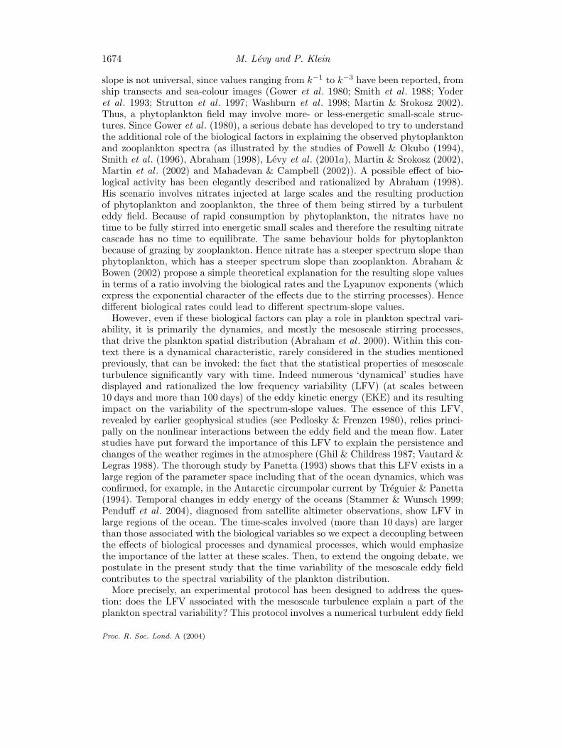
1674 M. Levy and P. Klein

slope is not universal, since values ranging from k−1 to k−3 have been reported, fromship transects and sea-colour images (Gower et al . 1980; Smith et al . 1988; Yoderet al . 1993; Strutton et al . 1997; Washburn et al . 1998; Martin & Srokosz 2002).Thus, a phytoplankton field may involve more- or less-energetic small-scale struc-tures. Since Gower et al . (1980), a serious debate has developed to try to understandthe additional role of the biological factors in explaining the observed phytoplanktonand zooplankton spectra (as illustrated by the studies of Powell & Okubo (1994),Smith et al . (1996), Abraham (1998), Levy et al . (2001a), Martin & Srokosz (2002),Martin et al . (2002) and Mahadevan & Campbell (2002)). A possible effect of bio-logical activity has been elegantly described and rationalized by Abraham (1998).His scenario involves nitrates injected at large scales and the resulting productionof phytoplankton and zooplankton, the three of them being stirred by a turbulenteddy field. Because of rapid consumption by phytoplankton, the nitrates have notime to be fully stirred into energetic small scales and therefore the resulting nitratecascade has no time to equilibrate. The same behaviour holds for phytoplanktonbecause of grazing by zooplankton. Hence nitrate has a steeper spectrum slope thanphytoplankton, which has a steeper spectrum slope than zooplankton. Abraham &Bowen (2002) propose a simple theoretical explanation for the resulting slope valuesin terms of a ratio involving the biological rates and the Lyapunov exponents (whichexpress the exponential character of the effects due to the stirring processes). Hencedifferent biological rates could lead to different spectrum-slope values.

However, even if these biological factors can play a role in plankton spectral vari-ability, it is primarily the dynamics, and mostly the mesoscale stirring processes,that drive the plankton spatial distribution (Abraham et al . 2000). Within this con-text there is a dynamical characteristic, rarely considered in the studies mentionedpreviously, that can be invoked: the fact that the statistical properties of mesoscaleturbulence significantly vary with time. Indeed numerous ‘dynamical’ studies havedisplayed and rationalized the low frequency variability (LFV) (at scales between10 days and more than 100 days) of the eddy kinetic energy (EKE) and its resultingimpact on the variability of the spectrum-slope values. The essence of this LFV,revealed by earlier geophysical studies (see Pedlosky & Frenzen 1980), relies princi-pally on the nonlinear interactions between the eddy field and the mean flow. Laterstudies have put forward the importance of this LFV to explain the persistence andchanges of the weather regimes in the atmosphere (Ghil & Childress 1987; Vautard &Legras 1988). The thorough study by Panetta (1993) shows that this LFV exists in alarge region of the parameter space including that of the ocean dynamics, which wasconfirmed, for example, in the Antarctic circumpolar current by Treguier & Panetta(1994). Temporal changes in eddy energy of the oceans (Stammer & Wunsch 1999;Penduff et al . 2004), diagnosed from satellite altimeter observations, show LFV inlarge regions of the ocean. The time-scales involved (more than 10 days) are largerthan those associated with the biological variables so we expect a decoupling betweenthe effects of biological processes and dynamical processes, which would emphasizethe importance of the latter at these scales. Then, to extend the ongoing debate, wepostulate in the present study that the time variability of the mesoscale eddy fieldcontributes to the spectral variability of the plankton distribution.

More precisely, an experimental protocol has been designed to address the ques-tion: does the LFV associated with the mesoscale turbulence explain a part of theplankton spectral variability? This protocol involves a numerical turbulent eddy field

Proc. R. Soc. Lond. A (2004)

Plankton spectral variability 1675

500 1000 1500 20000days

0

50

100

150

200

250

0 200 400 600 800km

0

100

200

300

400

500

m2

s−2

m2

s−2

(a) (b)

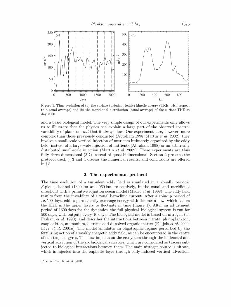
Figure 1. Time evolution of (a) the surface turbulent (eddy) kinetic energy (TKE, with respectto a zonal average) and (b) the meridional distribution (zonal average) of the surface TKE atday 2000.

and a basic biological model. The very simple design of our experiments only allowsus to illustrate that the physics can explain a large part of the observed spectralvariability of plankton, not that it always does. Our experiments are, however, morecomplex than those previously conducted (Abraham 1998; Martin et al . 2002): theyinvolve a small-scale vertical injection of nutrients intimately organized by the eddyfield, instead of a large-scale injection of nutrients (Abraham 1998) or an arbitrarilydistributed small-scale injection (Martin et al . 2002). These experiments are thusfully three dimensional (3D) instead of quasi-bidimensional. Section 2 presents theprotocol used, §§ 3 and 4 discuss the numerical results, and conclusions are offeredin § 5.

2. The experimental protocol

The time evolution of a turbulent eddy field is simulated in a zonally periodicβ-plane channel (1300 km and 960 km, respectively, in the zonal and meridionaldirection) with a primitive equation ocean model (Madec et al . 1998). The eddy fieldresults from the instability of a zonal baroclinic current. After a spin-up period ofca. 500 days, eddies permanently exchange energy with the mean flow, which causesthe EKE in the upper layers to fluctuate in time (figure 1). After an adjustmentperiod of 1600 days for the dynamics, the full physical–biological system is run for500 days, with outputs every 10 days. The biological model is based on nitrogen (cf.Fasham et al . 1990), and describes the interactions between nitrate, phytoplankton,zooplankton, ammonium, detritus and dissolved organic matter (Foujols et al . 2000;Levy et al . 2001a). The model simulates an oligotrophic regime perturbed by thefertilizing action of a weakly energetic eddy field, as can be encountered in the centreof sub-tropical gyres. The flow impacts on the ecosystem through the horizontal andvertical advection of the six biological variables, which are considered as tracers sub-jected to biological interactions between them. The main nitrogen source is nitrate,which is injected into the euphotic layer through eddy-induced vertical advection.



To assess the specific role of the biological interactions, a passive tracer, initializedwith uniform values of zero above and one below 100 m in order to mimic the nitratevertical gradient, was also considered. Therefore, the spatial heterogeneity of thispassive tracer is entirely set up by the dynamical processes, with vertical advectionacting as a source for the upper 100 m, and horizontal advection as a horizontalredistribution. The characteristics of the physical and biological models, as well asthose of the numerical simulations performed, are detailed in the appendix.

As expected, the time evolution of the surface EKE during the spin-up period(figure 1) is significant: after a transitory period of ca. 500 days, EKE fluctuates withtime-scales from 30 to 300 days and amplitude variations of up to 50%. At times,two zonal jets dominate the eddy field (figure 1), whereas eddies strongly dominateat other times. The intermittent appearance of these zonal jets is of course inti-mately related to the amplitude of the EKE relative to the mean-flow kinetic energy.This spatial distribution is a common feature of the nonlinear response of unstablebaroclinic jets (Panetta 1993). The next two paragraphs examine at a given timethe characteristics (in physical and spectral spaces) of the dynamical and biologicalvariables.

(a) Snapshots of the turbulent eddy field

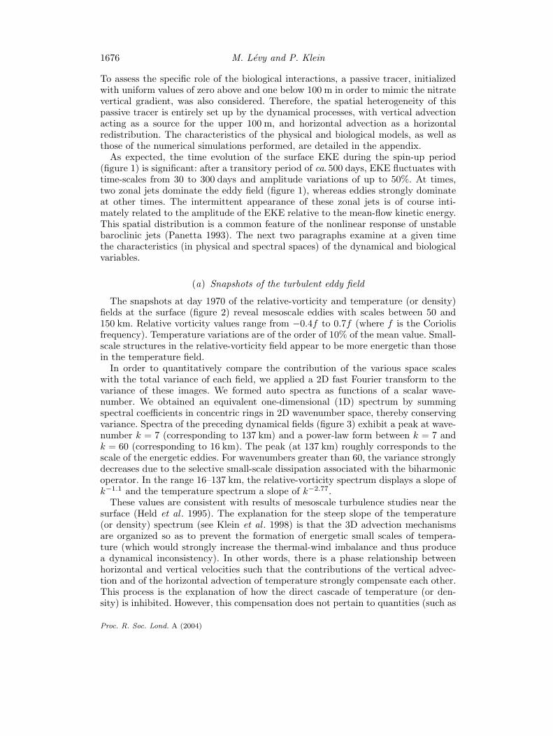
The snapshots at day 1970 of the relative-vorticity and temperature (or density)fields at the surface (figure 2) reveal mesoscale eddies with scales between 50 and150 km. Relative vorticity values range from −0.4f to 0.7f (where f is the Coriolisfrequency). Temperature variations are of the order of 10% of the mean value. Small-scale structures in the relative-vorticity field appear to be more energetic than thosein the temperature field.

In order to quantitatively compare the contribution of the various space scaleswith the total variance of each field, we applied a 2D fast Fourier transform to thevariance of these images. We formed auto spectra as functions of a scalar wave-number. We obtained an equivalent one-dimensional (1D) spectrum by summingspectral coefficients in concentric rings in 2D wavenumber space, thereby conservingvariance. Spectra of the preceding dynamical fields (figure 3) exhibit a peak at wave-number k = 7 (corresponding to 137 km) and a power-law form between k = 7 andk = 60 (corresponding to 16 km). The peak (at 137 km) roughly corresponds to thescale of the energetic eddies. For wavenumbers greater than 60, the variance stronglydecreases due to the selective small-scale dissipation associated with the biharmonicoperator. In the range 16–137 km, the relative-vorticity spectrum displays a slope ofk−1.1 and the temperature spectrum a slope of k−2.77.

These values are consistent with results of mesoscale turbulence studies near thesurface (Held et al . 1995). The explanation for the steep slope of the temperature(or density) spectrum (see Klein et al . 1998) is that the 3D advection mechanismsare organized so as to prevent the formation of energetic small scales of tempera-ture (which would strongly increase the thermal-wind imbalance and thus producea dynamical inconsistency). In other words, there is a phase relationship betweenhorizontal and vertical velocities such that the contributions of the vertical advec-tion and of the horizontal advection of temperature strongly compensate each other.This process is the explanation of how the direct cascade of temperature (or den-sity) is inhibited. However, this compensation does not pertain to quantities (such as



units of f

200 400 600 800 1000 1200km

0

200

400

600

800km

−0.10 −0.06 −0.02 0.02 0.06 0.10

ºC

0 200 400 600 800 1000 1200km

−1.00 −0.60 −0.20 0.20 0.60 1.00

mmole N m−2

200 400 600 800 1000 1200km

0

200

400

600

800

km

5 6 7 8 9 10

mmole N m−2

0 200 400 600 800 1000 1200km

3.0 3.8 4.6 5.4 6.2 7.0

(a) (b)

(c) (d)

Figure 2. Snapshots at day 1970 of (a) surface relative vorticity, (b) surface-temperature anomaly(with respect to the zonal mean), (c) 0–150 m phytoplankton and (d) 0–150 m zooplankton.

relative vorticity or any passive tracer) whose initial conditions (and forcing terms)differ from those of temperature. In that case, the direct cascade from large to smallscales is efficient, and produces energetic small scales.

(b) Snapshots of the plankton fields

Figure 2 displays a snapshot at day 1970 of the phytoplankton and zooplanktonfields, integrated from the surface down to 150 m. Indeed, a characteristic of theoligotrophic regime is that plankton maxima remain at sub-surface, and at a depththat varies with the intensity of the nitrate injection. Therefore, in order to focuson the horizontal patchiness, our analyses are performed on vertically integratedplankton fields over the top 150 m.

The ratio between the minimum and maximum phytoplankton concentrations isof the order of three. The same ratio is found for zooplankton. The plankton fieldshave spatial characteristics much closer to those of relative vorticity than to those



k−1.1 k−2.77

k−1.36

k−1.39

10 100wavenumber k

10−8

10−6

10−4

10−2

log

(var

ianc

e)

k−0.99

10 100wavenumber k

10 100wavenumber k

10−8

10−6

10−4

10−2

log

(var

ianc

e)

(a) (b) (c)

(d) (e)

10 100wavenumber k

10 100wavenumber k

Figure 3. Variance spectra of the fields displayed in figure 2 ((a) surface relative vorticity,(b) temperature, (c) 0–150 m phytoplankton and (d) 0–150 m zooplankton) and of (e) a passivetracer (integrated over 0–150 m). Slopes, estimated from linear regressions between wavenumbers8 and 50, are also drawn.

of temperature. Qualitatively, figure 2 shows that plankton and relative-vorticityfields exhibit energetic sub-mesoscale features at the same locations. A quantitativeanalysis of that correspondence in the next paragraph will also reveal that the phaseof the small-scale structures in plankton and vorticity are coherent, with planktonbeing more abundant in negative-vorticity filamentary structures.

Plankton and passive-tracer spectra (figure 3) exhibit a peak at the same wave-number as that for the dynamical variables (i.e. at k = 7). The passive-tracer field(also integrated between 0 and 150 m) displays a spectrum slope close to the theoret-ical value (k−0.99). The biological spectrum slopes differ slightly from those of therelative vorticity and of the passive-tracer fields: phytoplankton has a k−1.36 slopeand zooplankton a k−1.39 slope. As Abraham’s (1998) experiments suggest, thesevalues are likely to be sensitive to the biological rates. One now has to address thequestion of this study, i.e. whether these plankton spectrum slopes are steady intime and, if not, what makes them vary (since, in our simulation, biological rates areconstant). An examination of the time-series of the different variables over 500 days,given in § 3, will provide an answer to this question.

3. Results over 500 days

The 500 days of the simulation (after the adjustment period of 1600 days) revealthat the preceding spectral characteristics of the dynamical and biological fields are



Table 1. Statistics on spectral slopes

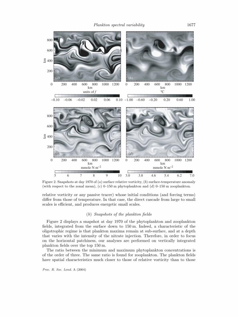
(For relative vorticity and temperature, slopes are computed from surface fields. For phytoplank-ton, zooplankton and the passive tracer, the slopes are computed on the 0–150 m integratedfields. For each field, 50 snapshots are available, and spectral analysis is performed on eachsnapshot. The mean slope is the mean respective to the ensemble of snapshots. The standarddeviation is respective to that of the mean. The minimum and maximum are the extremumslope values obtained among the 50 snapshots.)

standardmean maximum minimum deviation

relative vorticity −1.64 −1.2 −2.1 0.15temperature −3.17 −2.8 −3.5 0.15phytoplankton −1.50 −1.2 −1.7 0.11zooplankton −1.65 −1.2 −2.1 0.18passive tracer −1.42 −1.0 −1.7 0.17

not steady. Instead, they strongly vary with time. Furthermore, they show that thetime variability of plankton spatial distribution is mostly driven by the dynamicalfields. A persistent signature of this dynamical guidance is the strong resemblance, inphysical space, between plankton and relative-vorticity patterns: at any time duringthese 500 days, phytoplankton and zooplankton concentrations are mostly enhancedin negative-vorticity structures.

(a) Spectral characteristics

The time variability of the patchiness of physical and biological variables is assessedby calculating the corresponding spectra for each of the 50 available snapshots (oneevery 10 days for 500 days). Consistent with the results for the EKE (figure 1), spec-trum slopes reveal a significant LFV (figure 4). As before, the spectrum slopes arecomputed by applying linear regressions between wavenumbers 10 and 50. Remark-ably, the standard deviation on the linear regressions never exceeds 5% although thevalues of the spectral slopes show strong temporal variation. Moreover, we evaluatethe absolute error in the computation of the slope due to the choice of the wave-number range (in the larger limit k = 7 to k = 60) to be ±0.1. The relative results(comparison between slopes of different variables) do not depend on the exact choiceof the wavenumber range, provided that the same range is used for all variables.

The mean spectral slope (over 500 days) for surface relative vorticity is −1.64,but the extremum values are −1.2 and −2.1, with a standard deviation of 0.15 (seetable 1). The mean passive tracer spectrum slope (−1.42) is flatter than the meanrelative vorticity spectrum slope. The phytoplankton spectrum slope lies between thetwo: its range is between −1.2 and −1.7 with a mean value of −1.5. The temperaturespectrum slope is of course much steeper and ranges between −2.8 and −3.5 with amean value of −3.17. These values are consistent with observations (see, for example,Martin & Srokosz 2002).

Relative vorticity, temperature, phytoplankton and passive tracer spectral slopesshow LFV (figure 4) on time-scales of the order of 30–100 days (the case for zooplank-ton is discussed later). A very important peculiarity is that the phase of this variabil-ity is about the same for all biological and dynamical fields. Except for zooplankton,



1600 1700 1800 1900 2000 2100days

−4

−3

−2

−1

relative vorticitytemperature

phyto.zoo.passive tracer

−40 −20 0 20 40time lag in days

RV/temp.RV/phyto.RV/zoo.RV/PT

(a) (b)

−0.2

0.0

0.2

0.4

0.6

0.8

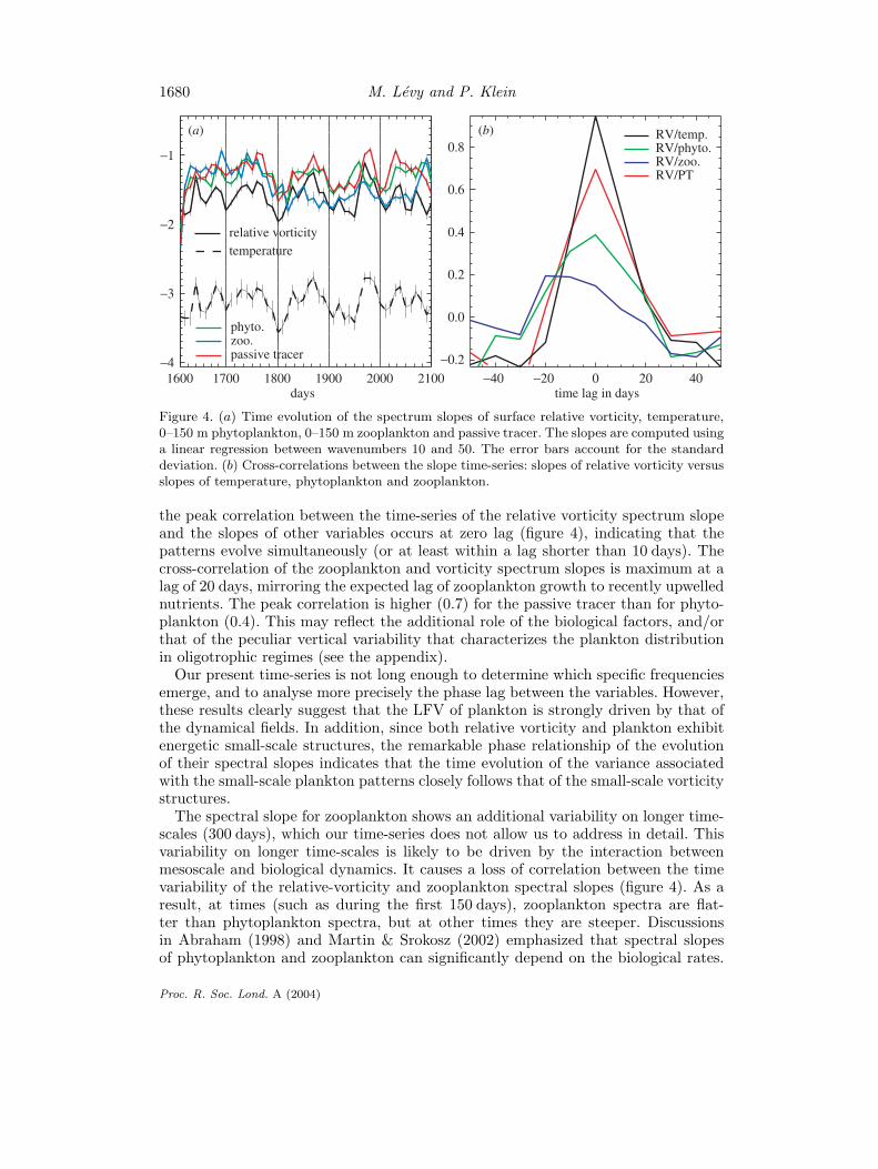
Figure 4. (a) Time evolution of the spectrum slopes of surface relative vorticity, temperature,0–150 m phytoplankton, 0–150 m zooplankton and passive tracer. The slopes are computed usinga linear regression between wavenumbers 10 and 50. The error bars account for the standarddeviation. (b) Cross-correlations between the slope time-series: slopes of relative vorticity versusslopes of temperature, phytoplankton and zooplankton.

the peak correlation between the time-series of the relative vorticity spectrum slopeand the slopes of other variables occurs at zero lag (figure 4), indicating that thepatterns evolve simultaneously (or at least within a lag shorter than 10 days). Thecross-correlation of the zooplankton and vorticity spectrum slopes is maximum at alag of 20 days, mirroring the expected lag of zooplankton growth to recently upwellednutrients. The peak correlation is higher (0.7) for the passive tracer than for phyto-plankton (0.4). This may reflect the additional role of the biological factors, and/orthat of the peculiar vertical variability that characterizes the plankton distributionin oligotrophic regimes (see the appendix).

Our present time-series is not long enough to determine which specific frequenciesemerge, and to analyse more precisely the phase lag between the variables. However,these results clearly suggest that the LFV of plankton is strongly driven by that ofthe dynamical fields. In addition, since both relative vorticity and plankton exhibitenergetic small-scale structures, the remarkable phase relationship of the evolutionof their spectral slopes indicates that the time evolution of the variance associatedwith the small-scale plankton patterns closely follows that of the small-scale vorticitystructures.

The spectral slope for zooplankton shows an additional variability on longer time-scales (300 days), which our time-series does not allow us to address in detail. Thisvariability on longer time-scales is likely to be driven by the interaction betweenmesoscale and biological dynamics. It causes a loss of correlation between the timevariability of the relative-vorticity and zooplankton spectral slopes (figure 4). As aresult, at times (such as during the first 150 days), zooplankton spectra are flat-ter than phytoplankton spectra, but at other times they are steeper. Discussionsin Abraham (1998) and Martin & Srokosz (2002) emphasized that spectral slopesof phytoplankton and zooplankton can significantly depend on the biological rates.



RV, day 2040

200 300 400 500km

300

400

500

600

km

−0.20 −0.12 −0.04 0.04 0.12

units of f

phyto., day 2040

200 300 400 500km

5 6 7 8 9 10

mmole N m−2

zoo., day 2040

200 300 400 500km

3.0 3.6 4.2 4.8 5.4 6.0

mmole N m−2

RV, day 2070

1000 1100 1200km

500

600

700

800

km

phyto., day 2070

1000 1100 1200km

zoo., day 2070

1000 1100 1200km

0.20

(e) ( f )

(a) (b) (c)

(d )

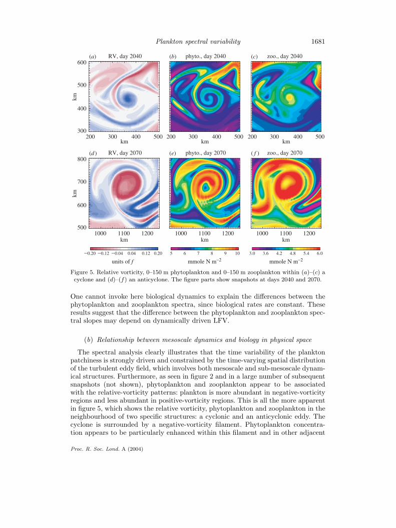
Figure 5. Relative vorticity, 0–150 m phytoplankton and 0–150 m zooplankton within (a)–(c) acyclone and (d)–(f) an anticyclone. The figure parts show snapshots at days 2040 and 2070.

One cannot invoke here biological dynamics to explain the differences between thephytoplankton and zooplankton spectra, since biological rates are constant. Theseresults suggest that the difference between the phytoplankton and zooplankton spec-tral slopes may depend on dynamically driven LFV.

(b) Relationship between mesoscale dynamics and biology in physical space

The spectral analysis clearly illustrates that the time variability of the planktonpatchiness is strongly driven and constrained by the time-varying spatial distributionof the turbulent eddy field, which involves both mesoscale and sub-mesoscale dynam-ical structures. Furthermore, as seen in figure 2 and in a large number of subsequentsnapshots (not shown), phytoplankton and zooplankton appear to be associatedwith the relative-vorticity patterns: plankton is more abundant in negative-vorticityregions and less abundant in positive-vorticity regions. This is all the more apparentin figure 5, which shows the relative vorticity, phytoplankton and zooplankton in theneighbourhood of two specific structures: a cyclonic and an anticyclonic eddy. Thecyclone is surrounded by a negative-vorticity filament. Phytoplankton concentra-tion appears to be particularly enhanced within this filament and in other adjacent



−0.4 −0.2 0 0.2 0.4relative vorticity (units of f )

7.0

7.5

8.0

8.5

9.0

9.5

phyt

opla

nkto

n (m

mol

e N

m−2

)

−0.4 −0.2 0 0.2 0.4relative vorticity (units of f )

−2

0

2

4

vert

ical

vel

ocity

(m

d−1

)(a) (b)

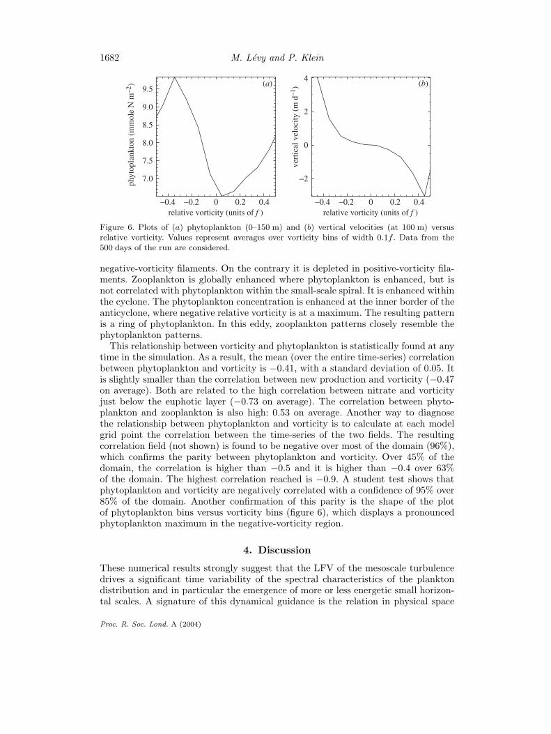
Figure 6. Plots of (a) phytoplankton (0–150 m) and (b) vertical velocities (at 100 m) versusrelative vorticity. Values represent averages over vorticity bins of width 0.1f . Data from the500 days of the run are considered.

negative-vorticity filaments. On the contrary it is depleted in positive-vorticity fila-ments. Zooplankton is globally enhanced where phytoplankton is enhanced, but isnot correlated with phytoplankton within the small-scale spiral. It is enhanced withinthe cyclone. The phytoplankton concentration is enhanced at the inner border of theanticyclone, where negative relative vorticity is at a maximum. The resulting patternis a ring of phytoplankton. In this eddy, zooplankton patterns closely resemble thephytoplankton patterns.

This relationship between vorticity and phytoplankton is statistically found at anytime in the simulation. As a result, the mean (over the entire time-series) correlationbetween phytoplankton and vorticity is −0.41, with a standard deviation of 0.05. Itis slightly smaller than the correlation between new production and vorticity (−0.47on average). Both are related to the high correlation between nitrate and vorticityjust below the euphotic layer (−0.73 on average). The correlation between phyto-plankton and zooplankton is also high: 0.53 on average. Another way to diagnosethe relationship between phytoplankton and vorticity is to calculate at each modelgrid point the correlation between the time-series of the two fields. The resultingcorrelation field (not shown) is found to be negative over most of the domain (96%),which confirms the parity between phytoplankton and vorticity. Over 45% of thedomain, the correlation is higher than −0.5 and it is higher than −0.4 over 63%of the domain. The highest correlation reached is −0.9. A student test shows thatphytoplankton and vorticity are negatively correlated with a confidence of 95% over85% of the domain. Another confirmation of this parity is the shape of the plotof phytoplankton bins versus vorticity bins (figure 6), which displays a pronouncedphytoplankton maximum in the negative-vorticity region.

4. Discussion

These numerical results strongly suggest that the LFV of the mesoscale turbulencedrives a significant time variability of the spectral characteristics of the planktondistribution and in particular the emergence of more or less energetic small horizon-tal scales. A signature of this dynamical guidance is the relation in physical space



between dynamical and biological variables, and particularly the good anticorrela-tion between vorticity and phytoplankton. One may wonder how to explain thisanticorrelation over such a large range of spatial scales.

To answer this question, one key point to take into account is that the whole bio-logical system is forced by the vertical advection. This remark allows us to makeuse of one of the results presented in Klein et al . (1998). Interestingly, Klein et al .(1998) found that a tracer forced by a large-scale negative vertical gradient is stronglyanticorrelated with the potential vorticity. Since the relative vorticity in the surfacelayers is very close to the potential vorticity, and since nitrate distribution is char-acterized by a strong negative vertical gradient, the dynamical arguments developedin Klein et al . (1998) are certainly pertinent in explaining the strong anticorrelation(−0.73) found in this study between vorticity and nitrate below the euphotic zone(which drives the anticorrelation between vorticity and phytoplankton, since nitrateis rapidly transformed into phytoplankton within the euphotic layer). In Klein etal . (1998), the dynamical characteristics of the mesoscale eddy field are set up (ashere) by both a large-scale vertical density gradient (the so-called stratification) anda large-scale horizontal density gradient (which makes the flow to be baroclinicallyunstable). During the nonlinear equilibration period, the physical system, to preventa thermal-wind imbalance (which would produce dynamical inconsistency), locallyorganizes the vertical and horizontal velocity fields such that vertical and horizon-tal advection of densities tend to compensate each other. This phase relationshipbetween vertical and horizontal advection (which also suggests that motions arealmost parallel to the isopycnals) explains that very few small-scale features arepresent in the density field, leading to a steep slope of the density spectrum. Thiscompensation between horizontal and vertical advection holds for any tracer forcedby the same large-scale vertical and horizontal gradients, but not for a tracer forcedby either the horizontal or the vertical gradient. In the last two cases, small scaleswill develop, and the consequence of the phase relationship is that a tracer forcedby a large-scale horizontal gradient will have its small scales strongly anticorrelatedto those of a tracer forced by a large-scale vertical gradient. To restate this argu-ment (see Klein et al . 1998 for details) more simply, motions (almost parallel to theisopycnals) are not an efficient mechanism for increasing density gradients, but areefficient enough to increase the gradients of properties whose isopleths are inclinedto the isopycnals. Vorticity and nitrate have their isopleths almost orthogonal (andtherefore both inclined to the isopycnals), since vorticity is forced by a large-scalehorizontal gradient and nitrate by a large-scale vertical gradient. This explains whysmall scales of vorticity should be strongly anticorrelated to those of nitrate, andultimately to those of phytoplankton, although a more thorough study is requiredto understand the additional contribution of the physics linked to the frontogenesisprocesses (not taken into account in Klein et al . (1998)). The results of Klein etal . (1998) also suggest another situation that is worth mentioning: since a traceronly forced by a large-scale horizontal gradient should be strongly correlated withthe potential vorticity, we can reasonably assume that the findings obtained in thepresent study should be similar (but strongly anticorrelated) to those from a situa-tion where plankton patchiness is forced by a large-scale nutrient injection involving alarge-scale horizontal gradient (i.e. not far from that described by Abraham (1998)).

A simpler (but less-physical and less-accurate) explanation of the strong anticor-relation between vorticity and plankton would invoke the equation for the relative



vorticity integrated in the surface layers: this equation is similar to that of a pas-sive tracer (as nutrients) forced by vertical advection, except for the sign of verticalvelocity. The plots of the ‘averaged values’ of phytoplankton against those of therelative vorticity, as well as those of the vertical velocity against those of the relativevorticity (figure 6), appear to confirm the preceding arguments.

5. Conclusion

The question addressed in this study was: does the LFV inherent to mesoscale tur-bulence explain a part of the spectral variability of plankton patchiness? The answerprovided by the results of our simple experiments is positive. The physics displaysa significant LFV (30–100 days) both in terms of the EKE (including the verticalvelocity variance) and of the spectral characteristics (i.e. the spatial distribution) oftemperature and vorticity. The same LFV characterizes the spatial heterogeneity ofthe biological variables. Furthermore, a significant phase relationship has been foundbetween the plankton spatial distribution and that of the relative vorticity. The spa-tial correlation between the physical and biological variables confirms the dominantrole of the physics in setting up the spatial variability of plankton distribution. Themechanisms in this study are more complex than those of previous studies, since theyinvolve nutrient input by the vertical pumping organized by the eddy field instead ofa large-scale vertical injection (Abraham 1998) or small-scale spots of vertical injec-tion with no precise phase relationship with the eddy field (Martin et al . 2002). Itis expected that the answer given by the results of the present study will still holdin the real world. They do not rule out the role of biological factors on the phyto-plankton and zooplankton spatial distributions. They suggest that this role can beassessed only when the part of LFV of the mesoscale eddy field is well estimated andremoved.

Anne-Marie Treguier is thanked for fruitful discussions. The OPA system team has made thiswork possible by maintenance of the OPA tracer code. Simulations were performed on the NEC-SX5 of the IDRIS centre. SAXO (developed by S. Masson) has been a great help in producingthe graphics. Funding for this study was provided by the French Ministere de la Recherche(through the ACI programme) and the CNRS (through the PROOF programme).

Appendix A. The numerical simulations

The primitive equation model OPA is used together with an embedded-ecosystemmodel (see Levy et al . 2001a) comprising six state variables (phytoplankton, zoo-plankton, nitrate, ammonium, dissolved organic matter and detritus). The domaingeometry is a flat, zonally periodic channel on a β plane, closed at the north andsouth boundaries, 960 × 1300 × 4 km3 centred at 35 ◦N. For the sake of simplicity,a linear equation of state is assumed (see Levy et al . 2001a). The initial state isa uniform meridional density gradient in hydrostatic and geostrophic balance. Thehorizontal density gradient covers a region of ca. 600 km width, and gives rise to aweak eastward flow with maximum velocities of 0.1 m s−1 at the surface. The meandensity profile yields a first baroclinic Rossby radius of deformation (that charac-terizes the scale of the mesoscale structures) of 30 km. The horizontal resolution is6 km. There are 30 z-coordinate vertical layers, whose thicknesses vary from 10 to20 m in the upper 100 m, and increase up to 300 m at the bottom. No wind nor net



surface heat forcing is accounted for. Energy is permanently injected into the systemon a large scale in the form of available potential energy. This is done by restoringdensity towards its initial frontal distribution. This density-forcing term takes theform γ × (ρ(x, y, z, t) − ρ(y, z)), where ρ(x, y, z, t) is the in situ density and ρ(y, z)is the initial density distribution. γ is set equal to 300 days−1, which correspondsto the life time of the longest-lived eddies and is long relative to the time-scales ofplankton. This restoring can be seen as the effect of a large-scale circulation thatwould maintain the large-scale density gradients on long time-scales. Free-slip con-ditions and no heat flux are applied along solid boundaries, except at the bottomwhere a linear friction drag is applied (equal to 4.6 × 10−4 m s−1). Vertical eddycoefficients are computed from an embedded 1.5 turbulent closure model. Horizon-tal mixing of density and momentum is included through biharmonic friction terms,with a dissipation coefficient |K| = 109 m4 s−1. The time-step is 16 min.

We have found in a previous modelling study (Levy et al . 2001a) that increasing thenumerical resolution from 6 km to 2 km significantly modifies the dynamical fields.This previous study investigated a much more energetic regime. The dissipationcoefficients associated with the 2 km and 6 km resolutions were |K2 km| = 0.5 ×109 m4 s−1 and |K6 km| = 35 × 109 m4 s−1. Therefore, in terms of dissipation, theregime of this study is closer (although slightly more dissipative) to the regime ofthe 2 km experiment of Levy et al . (2001a) than to that of the 6 km experiment. Wemay therefore expect to capture some aspects of the sub-mesoscale frontal dynamicswith a horizontal resolution of 6 km, which was not the case for the more energeticexperiments of Levy et al . (2001a). However, better representation of this small-scaledynamics would definitely require higher horizontal resolution. This was affordablein the case of the Levy et al . (2001a) experiments, which lasted for only 25 days andconcerned a much smaller domain. It would require enormous computer resources inthe present case.

The dynamical model is spun-up for 1600 days before the biological model isactivated for another 500 days. The initial conditions for the ecosystem are takenfrom a 1D configuration where only weak vertical diffusion is taken into account.The 1D configuration is run until an equilibrated oligotrophic situation is reached.In this equilibrated solution, the nitracline, phytoplankton and zooplankton sub-surface maxima are located at 110 m depth. This 1D solution is extended to thewhole domain, and is used as the initial condition for the 3D simulation. In the 3Dsolution, plankton maxima remain at the sub-surface, and, as expected for such aregime, at a depth that varies with the intensity of the nitrate injection. Therefore,in order to focus on the horizontal patchiness, we perform our analysis on verticallyintegrated plankton fields over the top 150 m.

Although it is preferable to use advection schemes that are positive and that min-imize dispersion for the transport of biological tracers at mesoscales (Levy et al .2001b), the centred advection scheme is used. This choice is made in order to usethe same numerics for the advection and diffusion of momentum, temperature andbiological tracers. By this we expect to minimize numerical artefacts in the com-parison between temperature, relative vorticity and phytoplankton variance spectra.Centred advection causes the generation of negative tracer values. Negative valuesare left negative, but are seen as zero for the computation of source–sink terms. Thefull dynamical-ecosystem simulation is carried out for 500 days. Model outputs areinstantaneous fields (snapshots) and have been saved every 10 days.



References

Abraham, E. R. 1998 The generation of plankton patchiness by turbulent stirring. Nature 391,577–580.

Abraham, E. R. & Bowen, M. M. 2002 Chaotic stirring by a mesoscale surface oceanic flow.Chaos 12, 373–381.

Abraham, E. R., Law, C. S., Boyd, P. W., Lavender, S. J., Maldonado, M. T. & Bowie, A. R.2000 Importance of stirring in the development of an iron-fertilized phytoplankton bloom.Nature 407, 727–730.

Fasham, M. J. R., Ducklow, H. W. & McKelvie, S. M. 1990 A nitrogen-based model of planktondynamics in the oceanic mixed-layer. J. Mar. Res. 48, 591–639.

Foujols, M.-A., Levy, M., Aumont, O. & Madec, G. 2000 OPA 8.1 Tracer model referencemanual. Note Technique du Pole de Modelisation du Climat. Paris, France: Institut PierreSimone Laplace (IPSL). (Available at http://www.ipsl.jussieu.fr).

Ghil, M. & Childress, S. 1987 Topics in geophysical fluid dynamics: atmospheric dynamics,dynamo theory and climate dynamics, p. 485. Springer.

Gower, J. F. R., Denman, K. L. & Holyer, R. L. 1980 Phytoplankton patchiness indicates theuctuations spectrum of mesoscale oceanic structure. Nature 288, 157–159.

Held, I. M., Pierrehumbert, R. T., Garner, S. T. & Swanson, K. L. 1995 Surface quasi-geostrophicdynamics. J. Fluid Mech. 282, 1–20.

Klein, P. & Hua, L. 1990 The mesoscale variability of the sea-surface temperature. An analyticaland numerical model. J. Mar. Res. 48, 729–763.

Klein, P., Treguier, A.-M. & Hua, B. L. 1998 Three-dimensional stirring of thermohaline fronts.J. Mar. Res. 56, 589–612.

Kraichnan, R. 1974 Convection of a passive scalar by a quasi-uniform random straining field. J.Fluid Mech. 64, 737–756.

Lapeyre, G., Klein, P. & Hua, B. L. 1999 Do tracer gradient vectors align with strain vectors in2D flows? Phys. Fluids 11, 3729–3737.

Levy, M., Klein, P. & Treguier, A.-M. 2001a Impacts of sub-mesoscale physics on phytoplanktonproduction and subduction. J. Mar. Res. 59, 535–565.

Levy, M., Estublier, A. & Madec, G. 2001b Choice of an advection scheme for biogeochemicalmodels. Geophys. Res. Lett. 28, 3725–3728.

Madec, G., Delecluse, P., Imbard, M. & Levy, C. 1998 OPA 8.1 Ocean general circulation modelreference manual. Note du Pole de Modelisation du Climat. Paris, France: Institut PierreSimone Laplace (IPSL). (Available at http://www.ipsl.jussieu.fr).

Mahadevan, A. & Campbell, J. W. 2002 Biogeochemical patchiness at the sea surface. Geophys.Res. Lett. 29, 1926–1929.

Martin, A. P. & Srokosz, M. A. 2002 Plankton distribution spectra: inter-size class variability andthe relative slopes for phytoplankton and zooplankton. Geophys. Res. Lett. 29, 2213–2216.

Martin, A. P., Richards, K. J., Bracco, A. & Provenzale, A. 2002 Patchy productivity in theopen ocean. Global Biogeochem. Cycles 16, No. 2, 10.1029/2001GB001449.

Panetta, R. L. 1993 Zonal jets in wide baroclinically unstable regions: persistence and scaleselection. J. Atmos. Sci. 50, 2073–2106.

Pedlosky, J. & Frenzen, C. 1980 Chaotic and periodic behavior of finite-amplitude baroclinicwaves. J. Atmos. Sci. 37, 1177–1196.

Penduff, T., Barnier, B., Dewar, W. K. & Brien, J. J. O. 2004 Impact of the North AtlanticOscillation on the oceanic eddy flow: dynamical insights from a model-data comparison. J.Phys. Oceanogr. (In the press.)

Powell, T. M. & Okubo, A. 1994 Turbulence, diffusion and patchiness in the sea. Phil. Trans.R. Soc. Lond. B343, 11–18.



Smith, K. S. & Vallis, G. K. 2001 The scales and equilibration of midocean eddies: freely evolvingflow. J. Phys. Oceanogr. 31, 554–571.

Smith, R. C., Zhang, X. & Michaelsen, J. 1988 Variability of pigment biomass in the Californiacurrent system as determined by satellite imagery. 1. Spatial variability. J. Geophys. Res. 93,10 863–10 882.

Smith, C. L., Richards, K. J. & Fasham, M. J. R. 1996 The impact of mesoscale eddies onphytoplankton dynamics in the upper ocean. Deep-Sea Res. I 43, 1807–1832.

Stammer, D. 1997 Global characteristics of ocean variability estimated from regional TOPEX/Poseidon altimeter measurements. J. Phys. Oceanogr. 27, 1743–1769.

Stammer, D. & Wunsch, C. 1999 Temporal changes in eddy energy of the oceans. Deep-Sea Res.II 46, 77–108.

Strutton, P. G., Mitchell, J. G., Parslow, J. S. & Greene, R. M. 1997 Phytoplankton patchiness:quantifying the biological contribution using fast repetition fluorometry. J. Plankton Res. 19,1265–1274.

Tennekes, H. & Lumley, J. L. 1972 A first course in turbulence, p. 300. Cambridge, MA: MITPress.

Treguier, A. M. & Panetta, R. L. 1994 Multiple zonal jets in a quasi-geostrophic model of theantarctic circumpolar current. J. Phys. Oceanogr. 24, 2263–2277.

Vautard, R. & Legras, B. 1988 On the source of mid-latitude low-frequency variability. II.Nonlinear equilibration of weather regimes. J. Atmos. Sci. 45, 2845–2867.

Washburn, L., Emery, B. M., Jones, B. H. & Ondercin, D. G. 1998 Eddy stirring and phyto-plankton patchiness in the subarctic North Atlantic in late summer. Deep-Sea Res. I 45,1411–1439.

Wunsch, C. 1997 The vertical partition of oceanic horizontal kinetic energy. J. Phys. Oceanogr.27, 1770–1794.

Yoder, J. A., Aiken, J., Swift, R. N., Hoge, F. E. & Stegmann, P. M. 1993 Spatial variability innear-surface chlorophyll a fluorescence measured by the airborne oceanographic lidar (AOL).Deep-Sea Res. II 40, 37–53.


Documents

Does the low frequency variability of mesoscale dynamics …marina/PUBLI/levy_klein_rs_04.pdf · Does the low frequency variability of mesoscale dynamics explain a part of the phytoplankton