Does the Sector Experience Affect the Pay Gap for ...doku.iab.de/veranstaltungen/2011/ws_flex2011_jahn_pozzoli.pdf · Does the Sector Experience A ect the Pay Gap for Temporary Agency

Does the Sector Experience Affect the PayGap for Temporary Agency Workers?∗

Elke Jahn∗

Institute for Employment Research and IZA

Dario Pozzoli‡

Aarhus School of Business, Aarhus University

Abstract

Usually temporary agency workers have to accept considerable wage penalties.However, remarkably little is known about the remuneration of workers whoare employed in this sector for a considerable length of time or accept temp jobsfrequently. Based on a rich administrative data set, we estimate the effects of theintensity of agency employment on the temp wage gap and post-temp earningsin Germany. Using a two-stage selection-corrected method in a dynamic paneldata framework, this article shows that the wage gap decreases with the timea workers spend in the sector be it at the same job or at different employers.This may be an indication that workers are able to accumulate human capital inthe sector which pays off in terms of remuneration. On the other hand, workerswho switch temp jobs on a frequent basis have to accept an even higher wagepenalty, which might be explained by stigma effects. Finally, temps who move topermanent jobs do not fully catch up to those who start in regular jobs in termsof remuneration.

Key words: Temporary Agency Employment, Treatment Intensity, Dose Re-sponse Function Approach, Wages, Germany.

JEL Classification: J30, J31, J42, J41.

∗We thank Sylvie Blasco and Boris Hirsch for helpful comments and suggestions. The usualdisclaimer applies.∗Corresponding Author : Institute for Employment Research Nuremberg (IAB), Aarhus School of

Business, Aarhus University and IZA, Regensburger Straße 148, 90478 Nuremberg, Germany. E-mail:[email protected]‡Aarhus School of Business, Department of Economics, Frichshuset, Hermodsvej 22, DK-8230,

Aabyhoj, Denmark, [email protected].

1 Introduction

This paper provides a comprehensive analysis of the remuneration of temporary agency

workers. Using a two-stage selection-corrected method in a dynamic panel data frame-

work, we explicitly take selection based on observable and unobservable characteristics

into account when estimating the pay gap of temporary agency employment. Moreover,

the literature so far concentrates on estimating the temp wage gap omitting that some

workers spend considerable time in agency employment. We show that the earnings

gap of agency workers depends on the experience in this sector or the ’treatment dose’.

Finally, we analyze whether the temp experience and its dose affects the earnings of

workers who move to a job outside the sector.

Investigating the working conditions and particularly the remuneration of agency

workers has become increasingly important as temporary agency employment has

turned out to be a significant employment form in most OECD countries during the

past decades. This trend has been particularly observed in Western Europe (Belgium,

France, Italy, The Netherlands, Spain, UK, Germany) and Japan. Germany, together

with the US and the UK, has become one of the largest markets in the world (CIETT,

2010). As temporary agency jobs are often regarded as ”bad jobs”, the expansion of

agency work raises concerns about labor market segmentation and dualism that trap

particular low-skilled workers in jobs providing little career prospect and poor pay.

The empirical evidence for continental European countries indicates indeed that the

average wage of temporary agency workers lags those of permanent workers by between

2 percent, in Portugal (Boheim and Cardoso, 2009) and 15 percent, in Germany (Jahn,

2

2010), after controlling for both observable and unobservable worker’s characteristics.

However, the temp wage gap is not only a continental European phenomenon. The

results provided by Segal and Sullivan (1998) and Addison et al. (2009) for the US,

Booth et al. (2002), Forde and Slater (2005) for the UK and Cohen and Haberfeld

(1993) for Israel confirm that temps have to accept a considerable pay penalty there

as well.1

As a consequence of the low wages in this sector not only most European govern-

ments but also the European commission feels the need to intervene. For example,

the European Parliament approved a Directive which stipulates equal pay of perma-

nent and agency workers in 2008. Member states can only derogate from the principle

of equal treatment if the workers are paid either by a collective agreement or by an

agreement between the national social partners (Eurofound, 2008).

However, agency employment might also have beneficial effects for the workers in

this sector which might compensate them for the lower pay. It is often argued that

some individuals may prefer to be employed in temp jobs rather than permanent jobs

as a career choice, to obtain or maintain eligibility for unemployment benefits or to

combine work with other activities or family responsibilities. Other individuals may

value temp jobs as a means of entering the labor market, securing an immediate source

of income while gaining work experience and human capital that can help them to

move up the job ladder or may even serve as a bridge into employment outside the

sector (e.g. Houseman et al. 2003). According to this hypothesis, the wage penalty

1To ease readability, we use the terms temp job or agency work interchangeably with temporaryagency employment and temp or agency worker instead of temporary agency worker.

3

temps experience is compensated for by the increased acquisition of human capital and

the development of productive job search networks (e.g. Autor, 2001).

Critics of this view claim that temporary agency work is unlikely to be conducive

to on-the-job training or networks, given its short job duration and low-skilled content

(Segal and Sullivan, 1997). Until today, the empirical evidence is rather mixed. While

some studies find that the experience of temporary agency employment improve sub-

sequent employment or wage outcomes (Ichino et al., 2008; Lane et al., 2003; Jahn and

Rosholm, 2010) others find no strong evidence for the stepping stone function of tempo-

rary agency work (Amuedo-Dorantes et al., 2008; Autor and Houseman, 2011; Garcıa-

Perez and Munoz-Bullon, 2005; Kvasnicka, 2009; Malo and Munoz-Bullon, 2008). An-

dersson et al.(2009), Hamersma and Heinrich (2008) and Heinrich et al. (2009) show

that temps are likely to have long-run earnings that are substantially below those who

transition to work in other sectors.

However, agency employment is rather heterogeneous. While some workers accept

only once an agency job during their employment career, for others it might be a career

choice as they are employed in this sector for a considerable length of time or accept

temp jobs on a frequent basis. If, as Autor (2001) argues, agencies provide workers

with free general skills training or if agency workers are able to improve their human

capital while being on assignment at different employers, one might suspect that the

pay gap for workers with an employment career inside the sector might be lower or

even dissipate. In this case concerns about the quality of agency jobs may be at least

for one part of the flexible staff unfounded.

4

Moreover, a longer employment experience in the agency sector might be valued

equivalently to an employment career outside the sector. The reason is that due to

their training within the sector and various assignments agency workers might be able

to acquire more human capital than workers being employed in other branches for a

given period of time (Autor, 2001). This may result in an increase of wages in post-

temp employment. Alternatively, a temp experience may stigmatize the worker in the

sense that future employers may perceive a previous temporary help job as an indicator

of lower ability and motivation. This negative signal may result in fewer job offers and

job opportunities with lower wages than other workers would receive (Blanchard and

Diamond 1994).

To shed more light on these competing hypotheses, this article gathers new evidence

for Germany, by estimating not only the wage differentials between temps and non-

temp workers as in the previous literature (Jahn, 2010), but also the effects on wages of

the ”intensity” or ”dose” of agency employment. The latter is measured either as the

cumulative number or the duration of past agency jobs. Conceiving temp employment

as a multi-valued treatment, allows us to directly test whether workers experiencing

higher exposures to temporary agency employment can indeed acquire more skills or

establish more productive job search networks which may result in an increase of wages

in the sector or in post-temp employment.

One of the most difficult issues in this literature is to take into account the self-

selection of workers into temporary agency employment (Autor 2009). Therefore the

observed market wages for different doses may still be the result of selection, even

5

after controlling for individual worker and job characteristics. To address the issue of

self-selection this paper applies a two-stage selection-corrected method in a dynamic

panel data framework, using a random sample drawn from the Integrated Employment

Biography (IEB) of the Institute for the Employment Research (IAB) for the period

2000-2008.

The worker’s assignment decision is examined first by either a dichotomous or a

polychotomous ordered probit model, depending on whether the binary or the multi-

value treatment is considered, in a reduced-form quarter by quarter setting. Over-time

variation, afforded by regional shares of temporary agency workers during our obser-

vation window, is exploited to identify an exogenous increase in the dose of temporary

agency employment which is unrelated to wages. The wage equations of different

treatment levels are then estimated by incorporating the possible selection bias terms

obtained in the ordered probit estimation. The treatment effects for different doses

of agency employment are than calculated from the estimation results. To investigate

the dose effect on wages further, we calculate the predicted wage path associated with

each treatment level for workers who move from temp to regular employment. As a

robustness check, we calculate the same effects implementing a matching estimator,

which allows for continuous treatment effect evaluation (Hirano and Imbens, 2004).

This study adds to the literature in this field in several respects. To the best

of our knowledge, this is the first time a dose-response function approach is applied

to a dynamic panel data setting. In this respect, we provide an extension of the

Chamberlain’s (1992) proposal in the spirit of the approach developed by Jimenez-

6

Martin (2006). Second, combined with a suitable IV-type identification strategy, our

econometric model allows us to fill a gap in the literature providing new evidence

about the causal impact of temporary agency employment intensity on wages and post-

temp wages. Third, by implementing an extension of the propensity-score matching

estimator in a setting with a continuous treatment, we are able to evaluate the effects

of intensity of agency employment over all possible values of the treatment levels.

This article shows that the wage gap decreases with the time a worker spend in

the sector be it at the same job or at different employers. Moreover, temps who move

to permanent jobs considerably reduce their gap with those who start in regular jobs

in terms of remuneration if they have spend more time in the agency sector. Both

results may be an indication that workers are able to accumulate human capital in

the agency sector which pays off in terms remuneration. However, workers who switch

temp jobs on a frequent basis have to accept a higher wage penalty and considerably

lower post-temp wages, which might reflect lower specific human capital investment or

might be explained by stigma effects.

The paper is organized as follows. Section 2 highlights key facts about the tem-

porary help sector in Germany. Section 3 introduces the data set and presents main

descriptive statistics. Section 4 provides details on the empirical strategy. Section

5 explains the results of our empirical analysis and section 6 offers some concluding

remarks.

7

2 Institutional background

Generally, temporary agency employment is characterized by a tripartite relationship,

whereby a temp worker is employed by a temp agency which then hires the worker

out under a commercial contract to perform a work assignment at a user firm. The

agency is considered to be the employer, determining issues such as wages and terms

of employment.

In Germany, agency employment is regulated by national legal statutes which ap-

ply only to temporary help agencies. Compared to international standards temporary

agency employment was highly regulated until the end of 2003. The main regulations

were: first, the maximum period of assignment, which determines how long a temp

may be assigned to a user firm without interruption, was 12 months. After this period

the agency had to provide the user firm with a different worker for the same task. Sec-

ond, although temporary help agencies were allowed to conclude fixed-term contracts,

a fixed-term contract could only be prolonged three times until total employment du-

ration added up to 24 months. Third, the agency was only allowed to conclude the

first employment contract for the duration of the first assignment. A second (or pro-

longed) employment contract with the same temp had to exceed the length of the next

assignment by at least 25 percent.2

The most recent reform, which came into effect in 2004 was intended to strengthen

the rights of temporary help workers by applying the principle of equal pay from the

2In 2002 the maximum period of assignment was extended to 24 months. Moreover, the principleof equal treatment from the 13th month of an assignment on was introduced. As workers are rarelyemployed more than six month at an agency, the reform did not have any practical effect (e.g. Antoniand Jahn, 2009).

8

first day of an assignment on. The new law allows deviation from the principle of

equal treatment if the agency applies the conditions stipulated in a sectoral collective

agreement to all its temp workers. As a consequence, wage gaps between temps and

the permanent staff of a user firm are permissible if the wages established in the user

firms collective agreement are higher than those in the temp industrys collective agree-

ment. In addition, by signing a collective agreement, the agency can free itself from all

other regulations. As a consequence, numerous collective agreements were concluded

in anticipation of this legal reform. By the end of 2003, nearly 97 percent of all tem-

porary help agencies paid their temps according to a sectoral collective agreement.

Consequently, the principle of equal treatment and all other regulations have lost any

practical meaning for the temporary help industry.

In contrast to many other countries where temps are exempted from mandated

social benefits, in Germany all workers have access to health insurance, sick, leave, hol-

iday leave, pension plans and work councils and are protected by statutory employment

protection legislation.

About 70 percent of all temps are male. As 90 percent of the temp jobs are full

time jobs, temps rarely are parallel employed in a non-temp job. Blue-collar occupa-

tions such as production jobs, security service, laborers and other low-skilled jobs are

dominant in this sector (Jahn 2010). The concentration of workers in this sector who

are at risk of marginalization in combination with evidence that the German metal

industry (e.g., automobile and aircraft industry) uses temps to circumvent the high

wages agreed upon in collective bargaining is one main reason while the remuneration

9

of agency workers is of key interest in the German policy debate about temporary

agency employment.

During our observation period the number of agency workers increased tremen-

dously from 277 thousand in January 2000 to 823 thousand in July 2008 and dropped

to 674 thousand by the end of 2008. Temporary agency employment constituted three

percent of the total dependent workforce and two percent of the overall workforce in

2008. The labor market flows suggest that the temporary help industry is even larger

than any stock figure or the industrys share would suggest. In 2008 about about 1,050

thousand new temporary agency jobs were concluded and, due to the crisis, 1,170 thou-

sand were terminated. In addition, the temporary help industry played an important

role in job creation in Germany: one out of four new jobs in 2007 was created in this

sector.

3 Data

3.1 Data description

Our empirical analysis is based on a 5 percent random sample of temporary agency

workers and a 0.5 percent sample of remaining workers drawn from the Integrated

Employment Biography (IEB) of the Institute for the Employment Research (IAB)

which covers the period 1975-2008. The IEB combines data from five different admin-

istrative sources (see Dorner et al. 2010 for details). This merged administrative data

set contains daily information about employment periods subject to social security

10

contributions, job seeking periods, participation in active labor market programs, and

periods during which the worker was eligible for unemployment assistance and ben-

efit. The IEB provides information on socio-economic and job characteristics at the

individual level. Being of an administrative nature, the IEB also provides longitudinal

information on the employment and unemployment history of employees. The IEB is

especially useful for analysis that take wages into account since the wage information

is used to calculate social security contributions and is therefore highly reliable.

Nevertheless, the IEB has some minor drawbacks. First, employment spells in tem-

porary help agencies are identified by an industry classification code. Consequently,

temporary agency workers cannot be distinguished from agencies permanent adminis-

trative staff which accounted for about five to seven percent of agency employees in

2003 depending on the size of the agency (Antoni and Jahn, 2009). Note also, as the

legal employer is the agency, we do not observe how often and in which sectors a worker

has been on assignment. Second, wages above the social security contribution ceiling

are top-coded. To address this problem we imputed wages above the social security

contribution ceiling using a heteroscedastic single imputation approach developed by

Buttner and Rassler (2008).3

Third, the IEB reports gross daily wages and does not provide information on hours

worked. We therefore exclude part-time employees, interns, and at-home workers from

the sample since the wage information is not comparable for these groups. For the same

3The regression is run separately by each year, gender and Eastern and Western German employees.In addition, we included the following control variables: age, age squared, nationality, six educationalgroups, industry codes, four variables for the occupational status, and eleven occupational variables,classifying the current position held by the worker, duration at the current job, duration of the currentjob squared, firm size and type of the region (metropolitan, urban, rural).

11

reason we exclude workers with wages below the social security contribution threshold.

Fourth, trainees are excluded as they belong to the agency staff and are not assigned

to user firms.

Fifth, the information on education is provided by employers. This means that

information on educational levels is missing for about 19 percent of the individuals.

We therefore imputed the missing information on education by employing a procedure

developed by Fitzenberger et al. (2005), which allows inconsistent education informa-

tion to be corrected over time as well. After applying this imputation procedure, we

had to drop about 4 percent of the individuals in the final data set due to missing or

inconsistent information on education.

The analysis is restricted to the period 1995 to 2008 and to non-agricultural em-

ployees between the ages of 18 and 60. We use the information for the period 1995

to 1999 to control for the employment career of the workers of the previous five years.

This allows estimating the wage equations for the period 2000 to 2008. To estimate the

wage differentials, we constructed a quarterly panel data set and included all workers

who were employed on June 30 of the respective year, but we took advantage of the

daily spell structure to construct the workers employment history.

3.2 Variables and Descriptive Statistics

The dependent variable is the log gross daily wage of the worker, which has been

deflated to 2005 levels using the CPI deflator. The binary treatment variable is an

indicator which is equal to one if a worker is employed at a temporary help service

12

agency and zero otherwise. The multi-valued treatment is instead measured either as

the cumulative number of weeks in temporary agency employment or the number of

agency jobs over the past 5 years. In a third specification, we also look at the number

of weeks spent in the current temp job.

As socio-demographic controls the following variables are included: gender, age, age

squared, citizenship, and education.4 The employment history is controlled for by the

previous labor force status (unemployed, long-term unemployed, not in the labor force,

employed as a temp and regular employed), whether the worker received previously

unemployment benefits, unemployment assistance or no benefits, the employment ex-

perience in weeks during the past five years, the number of regular and temp jobs

during the past 5 years and the uninterrupted previous employment duration in weeks.

As far as the current job is concerned, we differentiate between six occupational

groups: technical occupations with highly skilled workers, service occupations, clerical

occupations, manufacturing metal occupations, laborer and manufacturing other (see

Jahn 2010, for more details).

To account for the heterogeneity among the agencies, we include the age of the firm,

the firm size (5 classes), the share of female workers in the agency, the percentage of

temp agency employees with a university degree and with no vocational training. Fi-

nally, as macroeconomic variables, we consider the real annual growth rate of GDP, the

regional unemployment rate (based on 413 districts which form a local administrative

4Ethnic Germans are coded as foreigners because their human capital and employment historymay be closer to that of foreigners (Brucker and Jahn, 2011). Education has been classified usingthe following groups: Secondary degree without vocational training, secondary degree with vocationaltraining, high school degree without vocational training, high school degree with vocational training(base category), college, and university degree.

13

unit), a dummy indication whether the worker is employed in east or west Germany,

and three variables indicating whether a worker is employed in a metropolitan, urban,

or rural area.

Table 1 presents the means of basic socio-economic characteristics for temp and non-

temp workers which allows us to control for possible selection effects. In our analysis we

are able to include 5.1 million spells, among them 659 thousand temp work spells, and

278 thousand workers. About 20 percent of the temps and 19 percent of the non-temp

workers are employed in East Germany. On average temporary help workers earn less

than regular workers. The average daily real gross wage of temp workers is 53 Euros

during the observation period, the average wage for regular workers is 90 Euros.

Most temps are male. Compared to the share of foreigners in overall employment,

which on average amounts to 12 percent, foreigners are overrepresented in temps at

22 percent. The average age of temp workers (36 years) is lower than in the compar-

ison group (39 years). Workers with secondary degree and no vocational training are

overrepresented in temp employment (17 percent), compared to their share in regular

employment (9 percent). In contrast to most European countries, service jobs and

clerical occupations do not play an important role. About two thirds of all temps are

employed in manufacturing or as laborers. While about 54 percent of the temps were

previously unemployed, this is only true for 18 percent of the non-temps. More than

62 percent of the regular employed workers had been regularly employed before their

current job, which only holds for about 21 percent of the temp workers.

Table 1 also reveals that the employment career of temp workers is much more

14

fragmented. On average they changed the job about four times and accepted two temp

job five years prior to the present temp job. In contrast, workers which are currently

employed outside the temporary help sector switched their job twice on average and

barely have any temp experience.

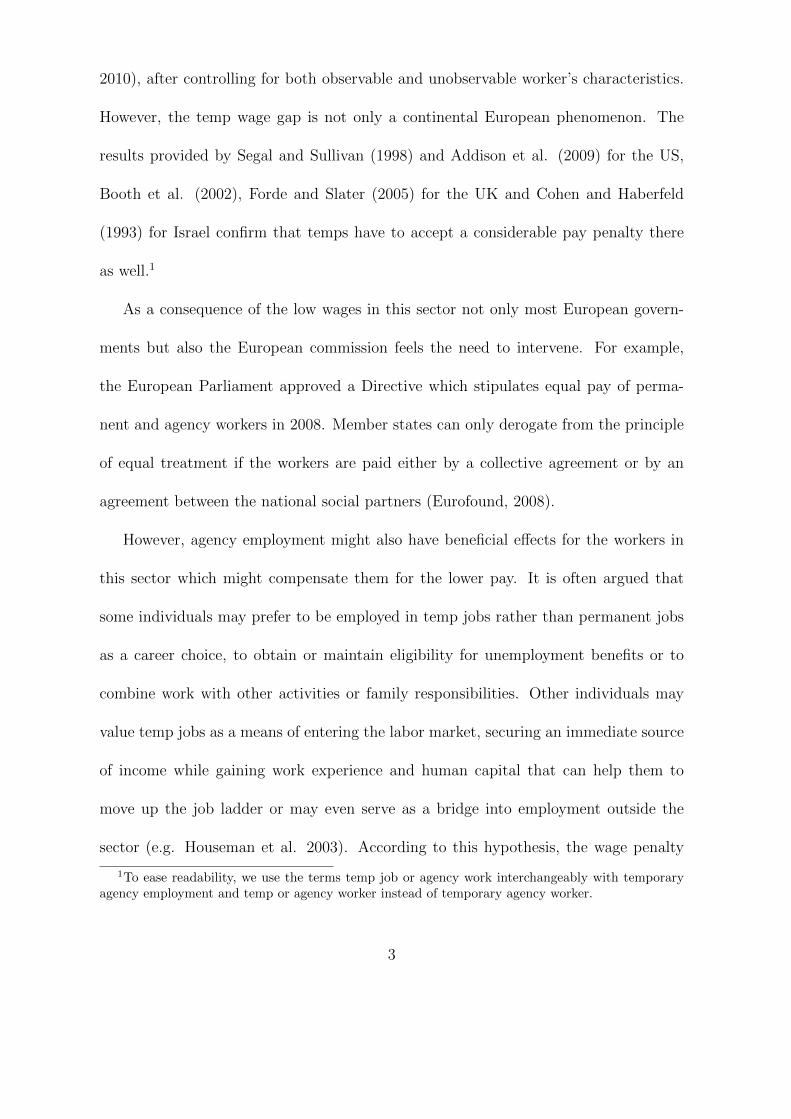
In order to get a first idea for the differences in mean wages between temps and

non-temp workers, we run OLS regressions separately for each year by gender and

region, which include only a dummy for being a temp worker as a control.

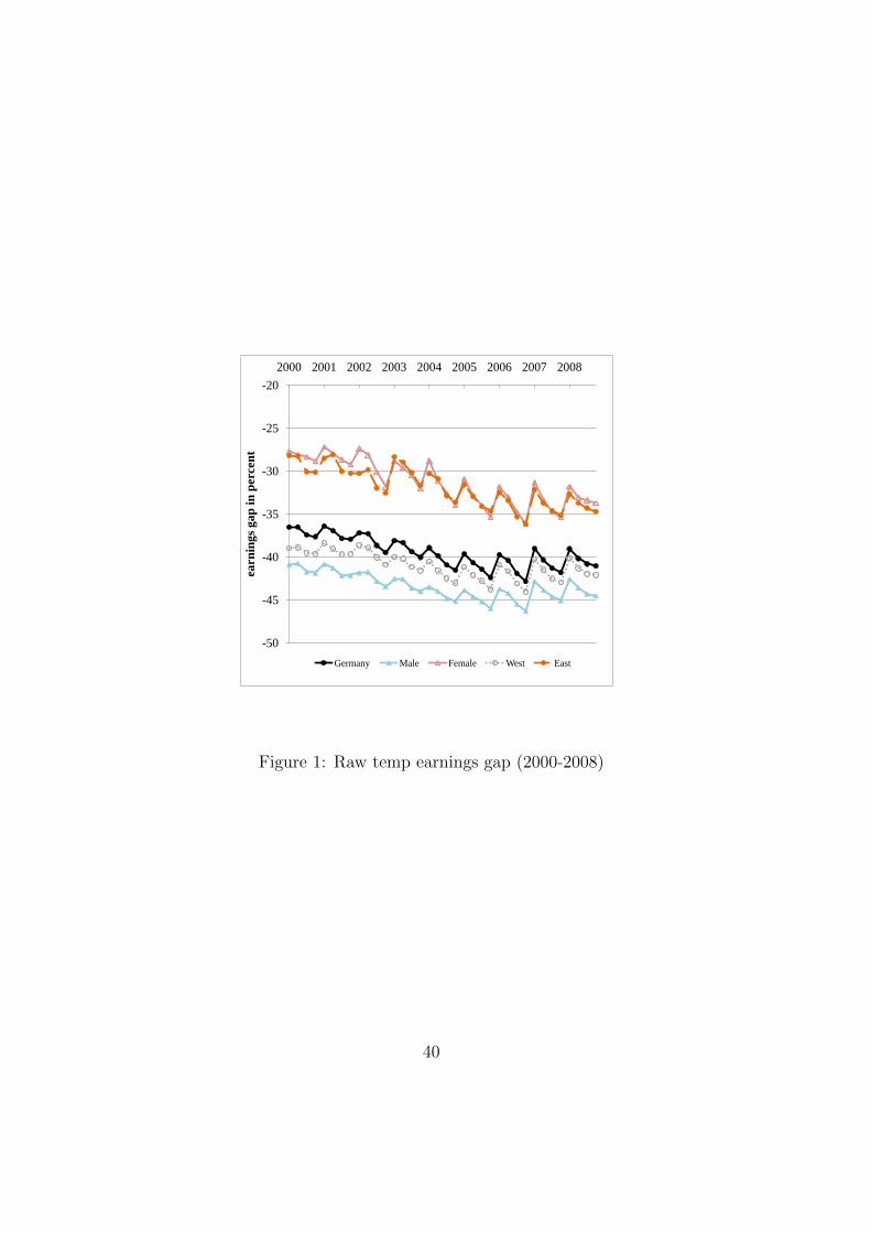
[Figure 1 about here]

The first striking result is that all wage differentials exhibits a downward trend

between 2000 and 2006. This result confirms earlier findings by Jahn (2010) who

found a widening earnings gap for the period 1997-2004 as well. Afterwards, the wage

gap decreases slightly for all groups, which might be a consequence of a tightening

labor market due to the upturn between 2007 and mid 2008. Figure 1 also reveals

that the wage differential for Eastern Germany is considerably lower than for Western

Germany and the wage gap for women is smaller than for man.

4 Empirical strategy

In this section we describe a consistent estimation procedure for the generalized dy-

namic sample selection model with panel data. Our point of departure is the following

two equation model5

5In our empirical analysis, we also consider the single equation version of the model discussed in

15

w0it = α0

0 +X′itα

01 + τt + µ0

i + e0it for t

0i s.t. Dit = 0

w1it = α1

0 +X′itα

11 + τt + µ1

i + e1it for t

1i s.t. Dit = 1

(1)

where wit is the log of the real daily wage for worker i in year t, X is a vector of

the observed worker and job characteristics described in the previous section, µ are

the time invariant individual specific effects and τ includes the GDP growth rate, the

unemployment rate and time dummies.6 The binary indicator D is the endogenous

treatment variable and determines whether the temps wage or the non-temps wage is

observed. The switching regime is driven by the model for D, which is given by:

D∗it = β0 + Z′

itβ2 + vit (2)

where the vector Z includes both a set of worker characteristics, i.e. gender, age,

citizenship, education, the employment history, whether the worker is living in East

Germany, and all the lags and the leads of the shares of temporary agency workers at

district level, which constitute our exclusion restrictions. The districts are clusters of

municipalities, which are grouped based on commuting patterns that can be interpreted

as self-containing labor markets. In total 413 local labor markets are identified. In our

opinion, they represent a more appropriate territorial configuration with respect to

larger administrative areas, like regions, to examine the interaction between workers

this section, which is given by: wit = α0 +X′

itα1 + τt + δdDit + µi + eit; i = 1, ...., N6Time dummies include the starting quarter of the job spell and a full set of quarter and year

dummies.

16

and potential externalities. The share of temporary agency workers at the commuting

area level presents a suitable supply driven instrument for the individual decision to

be a temporary agency worker herself which is not correlated with earnings.

In the equations of interest we should take into account that when cov(ekit, vit) 6= 0,

then neither E(e0it|s∗it ≤ 0) or E(e1

it|s∗it > 0) is expected to be zero. In order to control for

the endogenous selection problem, we estimate the parameters of the indicator equation

(2) and then, under the assumption of normality, which is not a crucial assumption

for the results to hold, we correct the equations of interest with corresponding inverse

Mill’s ratios.7 Adding consistent estimates of the inverse Mill’s ratios, λ0i and λ1

i to

equation (1), we obtain:

w0it = α0

0 +X′itα

01 + τt + ˆσ0λ0

i + µ0i + e0

it for t0i s.t. Dit = 0

w1it = α1

0 +X′itα

11 + τt + ˆσ1λ1

i + µ1i + e1

it for t1i s.t. Dit = 1

(3)

It is interesting to observe that under the structure imposed on the model, the

estimated coefficients of the inverse Mill’s ratios are informative on the presence and

direction of the selection process (σ0 for selection on unobserved ability or productiv-

ity and σ1 for the selection on the basis of their unobserved gain or of an unobserved

component in the treatment effect). Specifically, in the presence of an exclusion restric-

tion, like in our case, then the null of no selection on the unobservables can be tested

directly. In the framework above, this simply amounts to a test of the null hypothesis

7Following Jimenez-Martin’s (2006) we estimate a reduced-form quarter by quarter probit modelfor the agency employment decision.

17

that σ0 and σ1 are zero.

We consistently estimate equations (3) using the fixed effect estimator. Obviously,

the variance and covariance matrix of the two-step estimator needs to be adjusted for

the replacement of λ0i and λ1

i with λ0i and λ1

i by bootstrapping the sequential two-step

estimator.

We then extend the previous model by considering a multi-value treatment setting.

We measure the treatment intensity or dose either as the cumulative number or the

duration of past temp jobs over the last 5 years. In an alternative specification, we

also look at the number of weeks spent in the current temp job. The wage equations

for each level of treatment j are:

wjit = αj0 +X′

itαj1 + τt + µji + ejit for t

ji s.t. Dijt = 1; j = 0, 1, 2....m (4)

To cope with endogeneity issues, a quarter by quarter ordered probit model is

adopted to estimate the treatment choice equation. The dose-response function of the

optimal level of treatment can be expressed as:

DR∗ijt = γj0 + Z′

itγj1 + uijt (5)

The observed treatment dose is represented by a dummy variable Dijt and δ1, ....., δm

are cut-off points for the different treatment levels. Hence the probability of having

treatment level j becomes:

18

prob(Dijt = 1) = Φ(δj − γj0 − Z′

itγj1)− Φ(δj−1 − γj−1

0 − Z ′itγj−11 ) (6)

where Φ is a standard normal cumulative density function. Let ψij = σveσv

be the

covariance matrix of error terms between treatment dose choice and wage equations

and

λijt = E(uσu| δj−1−γj−1

0 −Z′itγj−11

σu< u

σu<

δj−γj0−Z′itγ

j1

σu

)=

φ(δj−1−γ

j−10 −Z

′itγ

j−11

σu)−φ(

δj−1−γj−10 −Z

′itγ

j−11

σu)

Φ(δj−1−γ

j−10 −Z′

itγj−11

σu)−Φ(

δj−1−Z′itγj−11

σu)

, 1 < j < m

(7)

be the expected value of the correction term. Then equation (4) can be rewritten

as:

wjit = αj0 +X′

itαj1 + τt + ψijλijt + µji + ejit for t

ji s.t. Dijt = 1; j = 0, 1, 2....m (8)

As before we estimate equation (7) using a two-stage estimator.

The estimation results obtained from the previous selection-corrected wage equa-

tions are used to calculate the implicit wage differential between different doses of

agency employment. The corrected differentials can generally be expressed as:

cdj =1

N

N∑i=1

T∑t=1

[E(wjit|Dijt = 1)− E(wj−1

it |Dij−1t = 1)]

(9)

where N is the number of individuals, wjit and wj−1it are predictions from the wage

equation (7), including the selection terms.

19

5 Results

5.1 Main Results

This section reports findings for each of the treatment dimensions we look at both

binary and multi-valued. Implementing both the single equation and the endogenous

switching approach helps in understanding the strength of our results.

Table 2 report results for the binary treatment from the single equation approach.

Whether the first row does not control for the selection into temporary agency em-

ployment, the second does. In line with the previous studies and with the descriptive

evidence, a negative effect of temporary agency employment is estimated. Interestingly,

the earnings gap slightly decreases from 19.6 to 18.8 percent, once the selection on un-

observables is taken into account. Separate estimates according to gender, to whether

the individual works in East or West Germany and to whether the period before or

after the 2003 reform is considered, indicate that women and workers in East Germany

suffer from a slightly lower wage penalties. Wage penalties are also reduced after the

2003 reform.8 Table A1 in the Appendix shows that the selection adjustment term

or the standard inverse Mills ratio is statistically significant and suggests a negative

selection bias.9 This implies that the estimated wage penalty is biased upward if the

sample selection bias is not controlled for. For this reason, we proceed presenting only

8The full set of regression coefficients for each group are available on request from the authors.9The control function approach requires an exclusion restriction. As mentioned before, all the

lags and the leads of the shares of temps at the district level where individuals works is used asinstruments. Besides the economic motivation for the instruments presented above, their statisticalvalidity is largely confirmed by the F-statistics reported in the footnotes below tables 2,3 and 4. TheF-statistics are always above 70, which allow us to clearly reject the null of weak instrument (Stockand Yogo, 2005).

20

the results obtained from the control function approach.

Tables 2 also summarizes the estimated effects of the multi-value treatments when

a single equation approach is implemented.10 If the treatment is measured in terms

of the number of weeks spent in temporary agency employment in the current job or

over the last 5 years, we find evidence that the estimated earning gaps are decreasing

with the treatment intensity. A temp worker who accumulates more than 52 weeks of

temporary agency employment in the current job (over the last 5 years) has a negative

wage gap of about 12 (14) percent with respect to a regular worker. The wage penalty

raises to about -20 (-18) percent if a temp worker with less than 8 weeks of agency

employment is considered. 11 Slightly lower temp wage differentials are estimated in

East Germany, after the 2003 reform is implemented and for women. These results

are in line with the hypothesis that temporary agency employment can be viewed as a

means of gaining work experience, human capital and labor market contacts that lead

to better wages. In this sense, we don’t find any evidence that spending more weeks

as a temp worker is interpreted as a negative signal or stigma in the labor market.

When we look at the number of temp jobs as treatment, however, lower and negligible

differences in the wage penalties are found across different number of treatments. To

sum up, it seems that the accumulated duration of temporary agency employment is

more relevant than the number of temp jobs in terms of the human capital that can be

accumulated in temporary agency employment. That the number of previous agency

10The full estimation results can be found in Table A2-A4.11Given that the single equation model is estimated exploiting the within variation through the

Fixed Effects method, the obtained effects are interpreted as the average effect of treatment on thetreated (ATT).

21

jobs has no effect in terms of remuneration might be an indication that accumulated

human capital can not be transfered between jobs. One possible explanation might be

that the human capital is firm or industry specific.

The results presented so far may be still questioned in terms of the assumptions im-

posed. The single equation model assumes in fact that the effects of temporary agency

employment do not vary across individuals. The endogenous switching model relaxes

the former assumption and allows the effect to be heterogeneous in both observable

and unobservable characteristics. To this end, we also estimate the wage equation for

each treatment regime separately and we augment it with the Mills ratios obtained

from the selection model, as described in the methodological section.

Table 3 reports the estimated wage equations for the treated and the non-treated

separately. The coefficients on most of the observable characteristics differ considerably

across temp and non-temp workers. If we look at the education variable, for example,

it is immediately apparent that its regression coefficients implies very different mag-

nitudes according to the employment regime. These findings warn against uncritical

aggregation by sector and indicate the presence of observable heterogeneity, we need

to take into consideration when the relevant treatment effects are estimated. More

importantly, the coefficient of the Mills ratio in the temporary agency wage equation

remains significant, indicating there is unobserved heterogeneity in the treatment effect

left, even after controlling for observed heterogeneity. As in the single equation ap-

proach, the coefficient of the Mills ratio in the temp sector indicates negative selection

in the same way we argued before. The results of Table 3 stress the need to allow

22

for observable heterogeneous returns in addition to selection on unobservables in our

application.12

The estimated ATTs from the endogenous switching model for both the binary and

multi-value treatments are summarized in Table 4. The calculated effects generally

involves greater magnitudes compared to the single equation model. Thus, for example,

a temp worker who accumulates more than 52 weeks of temporary agency employment

in the current job (over the last 5 years) has a negative wage gap of approximately

13 (17) percent with respect to a regular worker. The same wage gap increases to -40

(-35) percent for a temp with less than 8 weeks of agency employment. On the other

hand, the higher is the number of temp jobs, the larger the estimated wage gap with

respect to being in regular employment: having more than 3 distinct temporary agency

jobs over the last 5 years implies a significant negative wage gap of approximately 20

percent with respect to having just one temporary agency job. This again reinforces

the idea that human capital or the professional network can only be accumulated or

transfered if the worker is employed for longer period of time and probably in the same

firm or sector. Qualitatively similar results are obtained when the dose effects are

calculated separately by the relevant groups described before.

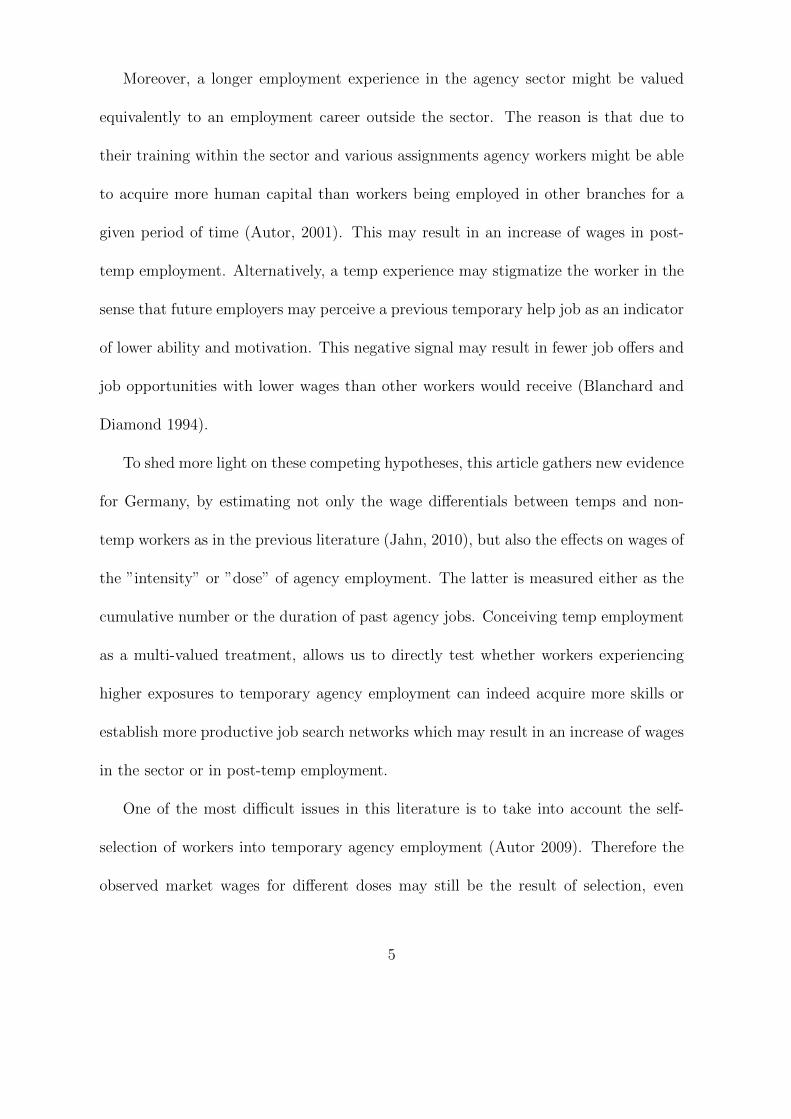
To describe the dose effect on wages further, we simulate alternative predicted wage

path for workers who move to regular employment with different levels of exposure to

the temp sector, either in terms of number or duration of past temp jobs. The patterns

involving workers with different number (duration) of past temp jobs are reported in

12Note, that Table A7 to A9 confirm the presence of observable heterogeneity also when multi-valuetreatment definitions are used.

23

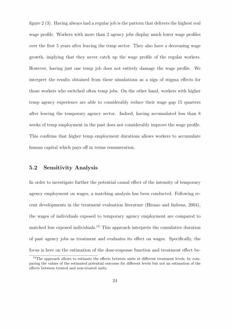
figure 2 (3). Having always had a regular job is the pattern that delivers the highest real

wage profile. Workers with more than 2 agency jobs display much lower wage profiles

over the first 5 years after leaving the temp sector. They also have a decreasing wage

growth, implying that they never catch up the wage profile of the regular workers.

However, having just one temp job does not entirely damage the wage profile. We

interpret the results obtained from these simulations as a sign of stigma effects for

those workers who switched often temp jobs. On the other hand, workers with higher

temp agency experience are able to considerably reduce their wage gap 15 quarters

after leaving the temporary agency sector. Indeed, having accumulated less than 8

weeks of temp employment in the past does not considerably improve the wage profile.

This confirms that higher temp employment durations allows workers to accumulate

human capital which pays off in terms remuneration.

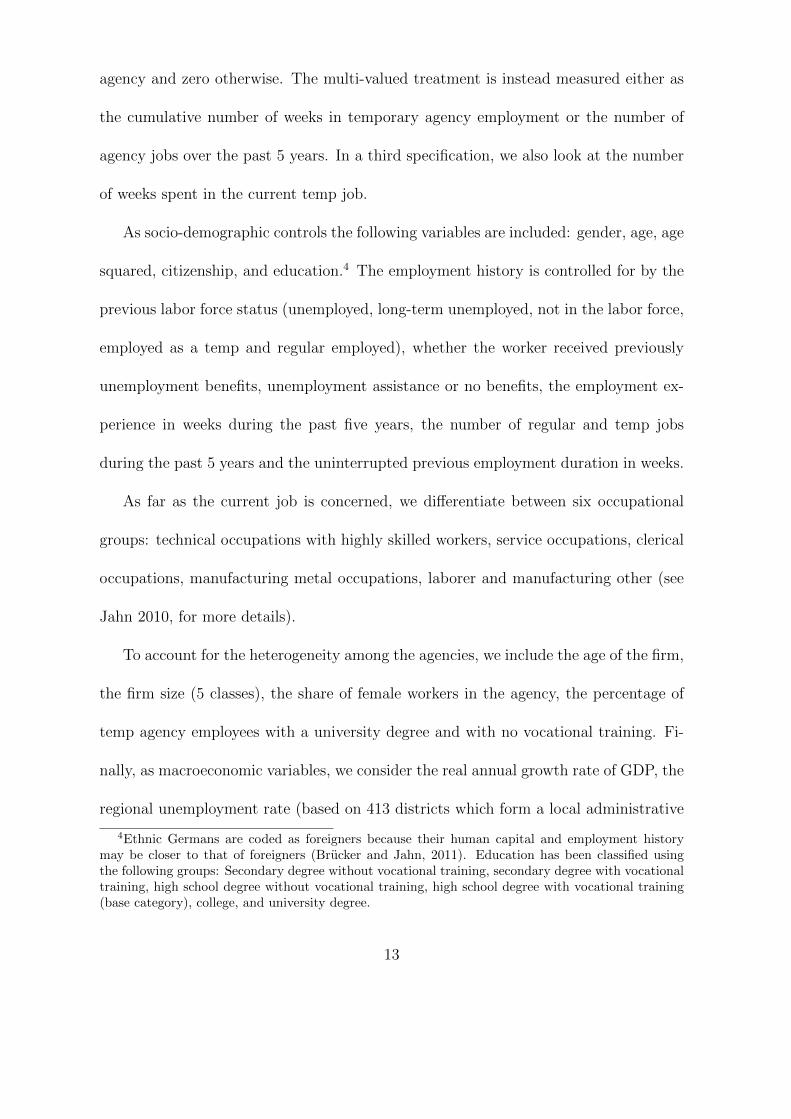
5.2 Sensitivity Analysis

In order to investigate further the potential causal effect of the intensity of temporary

agency employment on wages, a matching analysis has been conducted. Following re-

cent developments in the treatment evaluation literature (Hirano and Imbens, 2004),

the wages of individuals exposed to temporary agency employment are compared to

matched less exposed individuals.13 This approach interprets the cumulative duration

of past agency jobs as treatment and evaluates its effect on wages. Specifically, the

focus is here on the estimation of the dose-response function and treatment effect be-

13The approach allows to estimate the effects between units at different treatment levels, by com-paring the values of the estimated potential outcome for different levels but not an estimation of theeffects between treated and non-treated units.

24

havior. The implementation of such an analysis is also particularly important since it

may provide useful policy suggestions: it allows us to evaluate the impact of temporary

agency employment on wages for different level of exposure. The outcome variable (log

of wages) is taken in levels, the treatment is obviously the temporary agency employ-

ment experience over the last 5 years, measured in weeks. The matching variables

include all the observed worker and job characteristics used in equation (1). We also

add a set of time and quarter dummies to control for common aggregated demand and

supply shocks. Given the number of observations and available counterfactuals, it has

not been possible to estimate the effects for each quarter, so the latter are evaluated in

a pooled regression. To assess the balancing property, we divide the treatment variable

into terciles and test whether the GPS adjusted mean differs in one tercile compared

to the others.14

Figure 2 shows that the average dose-response functions increase with respect to

the level of treatment, confirming therefore the positive contribution of temporary

agency experience on wages. Doses of treatment produce significant responses when

the treatment reaches given levels in its distribution. Therefore, the experience effect

is increasing and statistically significant and it turns even stronger for high doses of

treatment. The average treatment effects are here defined respectively as the variation

in the estimated response function due to a 10 weeks increase (delta) in the treatment

14This is equivalent to testing that the conditional mean and treatment indicator are independent(CIA) where r(d;X) is evaluated at the median value of the treatment within the tercile d*. FollowingHirano and Imbens (2004), we test this hypothesis by blocking. For each tercile we define three blocksand compute the mean difference in X for observations (D=d) and (D>d). Then, we combine thesethree mean differences, weighted by the relative number of observations in each block, and computethe associated t-statistic value.

25

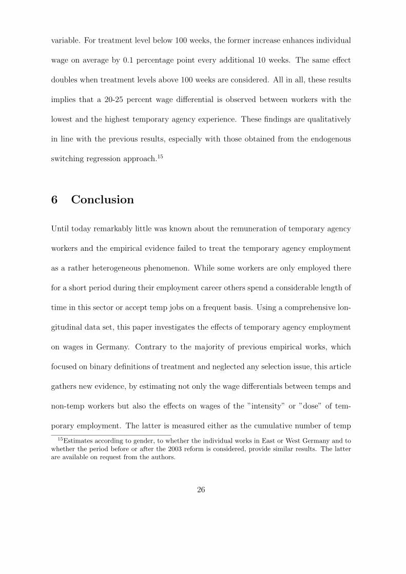
variable. For treatment level below 100 weeks, the former increase enhances individual

wage on average by 0.1 percentage point every additional 10 weeks. The same effect

doubles when treatment levels above 100 weeks are considered. All in all, these results

implies that a 20-25 percent wage differential is observed between workers with the

lowest and the highest temporary agency experience. These findings are qualitatively

in line with the previous results, especially with those obtained from the endogenous

switching regression approach.15

6 Conclusion

Until today remarkably little was known about the remuneration of temporary agency

workers and the empirical evidence failed to treat the temporary agency employment

as a rather heterogeneous phenomenon. While some workers are only employed there

for a short period during their employment career others spend a considerable length of

time in this sector or accept temp jobs on a frequent basis. Using a comprehensive lon-

gitudinal data set, this paper investigates the effects of temporary agency employment

on wages in Germany. Contrary to the majority of previous empirical works, which

focused on binary definitions of treatment and neglected any selection issue, this article

gathers new evidence, by estimating not only the wage differentials between temps and

non-temp workers but also the effects on wages of the ”intensity” or ”dose” of tem-

porary employment. The latter is measured either as the cumulative number of temp

15Estimates according to gender, to whether the individual works in East or West Germany and towhether the period before or after the 2003 reform is considered, provide similar results. The latterare available on request from the authors.

26

jobs or the duration of current or past temp jobs. Conceiving temporary employment

as a multi-valued treatment, allows us to directly test whether workers experiencing

higher exposures to temporary employment can indeed acquire more skills or establish

larger job search networks which may result in an increase of wages. As workers self-

select into different levels of treatment, the observed market wages for different doses

may still be the result of selection, even after controlling for individual worker and job

characteristics. For our analysis, we use a two-stage selection-corrected method in a

dynamic panel data framework. Over-time variation, afforded by regional shares of

temporary agency workers during our observation window, is exploited to identify an

exogenous increase in the dose of temporary agency employment which is unrelated to

wages.

In line with the previous study in this fields, the results show that agency workers

have to accept considerable lower wages. Interestingly, the earnings gap slightly de-

creases, once the selection on unobservables is taken into account. Our findings imply

that the estimated wage penalty is biased upward if the sample selection bias is not

controlled for.

When the treatment is measured in terms of the number of weeks spent in temporary

agency employment in the current job or over the last 5 years, we find evidence that the

estimated earning gaps are decreasing with the treatment intensity. Moreover, temps

who move to permanent jobs considerably reduce their gap with those who start in

regular jobs in terms of remuneration in case they have spend more time in the agency

sector. Both results may be an indication that workers are able to accumulate human

27

capital in the agency sector which pays off in terms remuneration. These results are

in line with the hypothesis that temporary agency employment can be viewed as a

means of gaining work experience or improving human capital that lead to better paid

jobs. This empirical evidence may also suggest that it may be inefficient for temporary

agency workers to invest in firm specific human capital, or for the employers to provide

this training unless the job has a longer term perspective.

This surmise is confirmed, when we look at the number of distinct temp jobs as

treatment. In this case the wage gap increases considerably with the number of treat-

ments, especially in the endogenous switching model. This may be again a consequence

of lower firm specific investment or training. Moreover, workers who frequently switch

between jobs might signal a lower productivity or that they are not wishing to remain

at the firm. Changing jobs too often might therefore be interpreted as a negative signal

that stigmatizes workers. Alternatively, agencies may pay these workers wages below

the productivity as they might lack an outside option. In this case, they are able to ex-

ercise monopsony control over the wages of workers filling the bottom tier of a two-tier

pay structure.

To sum up, this study confirms the popular perception that temporary agency jobs

are generally not desirable when compared to permanent employment, at least in term

of remuneration. This holds also for workers who are employed at the sector for a

considerable length of time, as the wage gap for these workers is still of an alarming

size. In light of the fact that agency employment in Germany is only rarely a pathway

into regular jobs (Kvasnicka 2009), these costs are not transitory. Consequently, the

28

boost of temporary agency employment in Germany during the last decade might not

only have increased labor market flexibility in Germany but has also created a two tier

labor market where a small part of the work force move regularly between unstable

jobs and are not financially compensated for taking that higher risk.

29

References

[1] Addison, J.; Cotti, C. and Surfield, Ch. (2009), Atypical Work: Who Gets It, and

Where Does It Lead? Some U.S. Evidence Using the NLSY79. IZA Discussion

Paper No. 4444, Bonn.

[2] Amuedo-Dorantes, C.; Malo, M. and Muoz-Bulln, F. (2008), ”The Role of Tempo-

rary Help Agency Employment on Temp-to-Perm Transitions,” Journal of Labor

Research 29: 138-161.

[3] Andersson, F.; Holzer, H. and Lane J. (2009), ”Temporary Help Agencies and the

Advancement Prospects of Low Earners.” In David Autor, ed., Studies in Labor

Market Intermediation, Chicago: The University of Chicago Press, 373-398.

[4] Antoni, M. and Jahn, E. (2009), Do Changes in Regulation Affect Employment

Duration in Temporary Work Agencies?. Industrial and Labor Relations Review

62: 226-251.

[5] Autor, D. (2001), Why Do Temporary Help Firms Provide Free General Skills

Training?. The Quarterly Journal of Economics 116: 1409-1448.

[6] Autor, D. and Houseman, S. (2011), Do Temporary Help Jobs Improve Labor

Market Outcomes for Low-Skilled Workers? Evidence from Work First. American

Economic Journal: Applied Economics, forthcoming.

30

[7] Bia, M. and Mattei, A. (2008), A Stata package for the estimation of the dose-

response function through adjustment for the generalized propensity score. The

Stata Journal 8: 354-373.

[8] Blanchard, O. and Diamond, P. (1994), ”Ranking, Unemployment Duration, and

Wages,” Review of Economic Studies 61: 417-434.

[9] Boheim, R. and Cardoso, A. (2009), Temporary help services employment in Por-

tugal. 1995-2000. In David Autor, ed., Studies in Labor Market Intermediation.

Chicago: The University of Chicago Press, 1-23.

[10] Booth, A.; Francesconi, M. and Frank J. (2002), Temporary Jobs: Stepping Stones

or Dead Ends?. Economic Journal, 112, F189-F213.

[11] Brucker, H. and Jahn, E. (2011), Migration and the Wage-Setting Curve: Reassess-

ing the Labor Market Effects of Migration, Journal of Scandinavian Economics,

forthcoming.

[12] Buttner, T. and Rassler, S. (2008), Multiple imputation of right-censored wages in

the German IAB employment register considering heteroscedasticity. In: United

States, Federal Committee on Statistical Methodology, (eds.), Federal Committee

on Statistical Methodology Research Conference 2007, Arlington.

[13] CIETT (2011). Agency work indicators. Online available: http://www.ciett.org.

[14] Chamberlain, G. (1992), Comment: sequential moment restrictions in panel data.

Journal of Business Economic Statistics, 10, 20-26.

31

[15] Cohen, Y. and Haberfeld, Y. (1993), Temporary Help Service Workers: Employ-

ment Characteristics and Wage Determination. Industrial Relations 32: 272-287.

[16] De Graaf-Zijl, M.; Van den Berg, G. and Hemya, A. (2011), ”Stepping Stones for

the Unemployed: The Effect of Temporary Jobs on the Duration until Regular

Work,” Journal of Population Economics 24: 107-139.

[17] Dorner, M.; Heining, J.; Jacobebbinghaus, P. and Seth, S. (2010), Sample of Inte-

grated Labour Market Biographies (SIAB) 1975-2008. FDZ Datenreport 01/2010.

Institute for Employment Research, Nuremberg, Germany.

[18] Eurofound (2008), Temporary agency work di-

rective approved. eiro-online. November 2008.

http://www.eurofound.europa.eu/eiro/2008/11/articles/eu0811029i.html.

[19] Forde, C. and Slater G. (2005), Agency work in Britain: character, consequences

and regulation. British Journal of Industrial Relations 43: 249-271.

[20] Fitzenberger, B.; Osikominu, A. and Volter, R. (2005), Imputation Rules to Im-

prove the Education Variable in the IAB Employment Subsample. ZEW Discussion

Paper No 05-10; Mannheim.

[21] Garcıa-Perez, J. and Munoz-Bullon, F. (2005), ”Are Temporary Help Agencies

Changing Mobility Patterns in the Spanish Labour Market?” Spanish Economic

Review 7: 43-65.

32

[22] Hamersma, S. and Heinrich, C. (2008), ”Temporary Help Service Firms’ Use of

Employer Tax Credits: Implications for Disadvantaged Workers’ Labor Market

Outcomes,” Institute for Research on Poverty, Discussion paper 1335-08, Wiscon-

sin.

[23] Heinrich, C.; Mueser, P. and Troske, K. (2009), ”The Role of Temporary Help

Employment in Low-wage Worker Ad-vancement.” In David Autor, ed., Studies

in Labor Market Intermediation, Chicago: The University of Chicago Press, 399-

436.

[24] Hirano, K. and Imbens, G. W. (2004), The Propensity Score with Continuous

Treatments. Working Paper, Department of Economics, University of California

at Berkeley.

[25] Houseman, S.; Kalleberg, A. and Erickcek, G. (2003), The Role of Temporary

Agency Employment in Tight Labor Markets. Industrial and Labor Relations Re-

view 57: 105-127.

[26] Ichino, A.; Mealli, F. and Nannicini, T. (2008), From Temporary Help Jobs to

Permanent Employment: What can we learn from matching estimators and their

sensitivity?. Journal of Applied Econometrics, 23, 305-327.

[27] Jahn, E. (2010), Reassessing the Pay Gap for Temps in Germany. Journal of

Economics and Statistic 230: 208-233.

33

[28] Jahn, E. and Rosholm, M. (2010), Looking beyond the bridge: How temporary

agency employment affects labor market outcomes. IZA Discussion Paper No.

4973, Bonn.

[29] Jimenez-Martin, S. (2006), Strike Outcomes and Wage Settlements in Spain,

LABOUR 20: 673-698.

[30] Kvasnicka, M. (2009), Does Temporary Agency Work Provide a Stepping Stone

to Regular Employment?. In David Autor, ed., Studies of Labor Market Interme-

diation, Chicago: The University of Chicago Press, 335-372.

[31] Lane, J.; Mikelson, K.; Sharkey, P. and Wissoker, D. (2003), ”Pathways to Work

for Low-Income Workers: The Effect of Work in the Temporary Help Industry,”

Journal of Policy Analysis and Management 22: 581-598.

[32] Malo, M. and Munoz-Bullon, F. (2008), ”Temporary help agencies and partici-

pation histories in the labour market: a sequence-oriented approach,” Estadstica

Espaola 50: 25- 65.

[33] Segal, L. and Sullivan, D. (1997), The Growth of Temporary Services Work. Jour-

nal of Economic Perspectives 11: 117-136.

[34] Segal, L. and Sullivan, D. (1998), Wage Differentials for Temporary Services Work:

Evidence from Administration Data. Federal Reserve Bank of Chicago. Working

Paper Series. No. WP-98-23. Chicago.

34

[35] Stock, J. H. and Yogo M. (2005), Testing for weak instruments in linear IV re-

gression. In D.W.K. Andrews and J.H. Stock (eds.), Identification amd inference

for econometric models: Essays in honour of Thomas Rothenberg, Cambridge:

Cambridge University Press.

35

Tables and Figures

Table 1: Descriptive statistics

Temp Non-tempmean sd mean sd

Average real gross wage 53 29 90 46Personal CharacteristicsAge 36 11 39 10Male 0.751 0.432 0.663 0.473Foreign 0.216 0.411 0.120 0.325East 0.203 0.402 0.191 0.393EducationSecondary degree no vt 0.170 0.376 0.089 0.285Secondary degree with vt 0.688 0.463 0.702 0.458High school degree no vt 0.008 0.091 0.007 0.086High school degree with vt 0.071 0.257 0.081 0.273Politechnics 0.029 0.168 0.046 0.209University 0.033 0.178 0.075 0.263Previous labor force statusUnemployed 0.536 0.499 0.183 0.386Long-term unemployed 0.084 0.278 0.025 0.156Not in the labor force 0.113 0.317 0.124 0.330Temporary employed 0.142 0.349 0.069 0.253Regular employed 0.210 0.407 0.624 0.484Previous benefitsUnemployment benefits 0.254 0.435 0.111 0.314Unemployment assistance 0.156 0.363 0.036 0.185Prev. empl. characteristisCurrent uninterrupted job tenure 82.900 85.800 184.000 95.200No temp jobs (5 years) 1.930 1.460 0.221 0.673No all jobs (5 years) 3.930 2.540 2.490 2.080Weeks in temp jobs (5 years) 85.900 79.800 6.830 24.100Weeks in non-temp jobs (5 years) 82.700 74.300 219.000 64.100OccupationTechnical occupation 0.032 0.176 0.078 0.269Manufacturing other 0.074 0.262 0.166 0.372Manufacturing metal sector 0.267 0.442 0.178 0.382Laborer 0.318 0.466 0.022 0.146Clerical occupation 0.148 0.355 0.352 0.478Service occupation 0.160 0.367 0.205 0.403Firm characteristicsFirmsize 0-10 0.020 0.140 0.153 0.360Firmsize 11-50 0.196 0.397 0.242 0.428Firmsize 51-200 0.519 0.500 0.247 0.431Firmsize 201-500 0.188 0.391 0.147 0.354Firmsize > 501 0.078 0.267 0.212 0.408Age of the firm (years) 10 7 18 11Share low skilled workers 26 27 9 15AgglomerationMetropolitan 0.567 0.495 0.546 0.498Urban 0.337 0.473 0.342 0.474Rural 0.096 0.295 0.112 0.316Regional unempl. rate (quarter) 11.500 4.650 11.000 4.980Observations 659,082 4,416,529

36

Table 2: Single equation approach, binary and multi-value treatments

Binary treatmentAll Men Women West East Before 2004 After 2004

FE –0.196*** –0.198*** –0.185*** –0.209*** –0.196*** –0.198*** –0.188***(0.000) (0.000) (0.001) (0.001) (0.000) (0.001) (0.001)

Control function approach –0.188*** –0.193*** –0.165*** –0.206*** –0.188*** –0.202*** –0.174***(0.001) (0.001) (0.002) (0.001) (0.001) (0.001) (0.001)

Multi value treatmentAll Men Women West East Before 2004 After 2004

Dose response function approach (1)Current temp job < 8 weeks –0.204*** –0.206*** –0.185*** –0.219*** –0.204*** –0.205*** –0.182***

(0.001) (0.001) (0.002) (0.001) (0.001) (0.001) (0.001)Current temp job 8-26 –0.180*** –0.183*** –0.159*** –0.194*** –0.180*** –0.184*** –0.161***

(0.001) (0.001) (0.002) (0.001) (0.001) (0.001) (0.001)Current temp job 26-52 –0.158*** –0.165*** –0.129*** –0.171*** –0.158*** –0.177*** –0.139***

(0.001) (0.001) (0.002) (0.001) (0.001) (0.001) (0.001)Current temp job > 52 –0.119*** –0.135*** –0.071*** –0.135*** –0.119*** –0.159*** –0.107***

(0.001) (0.001) (0.002) (0.001) (0.001) (0.002) (0.001)Dose response function approach (2)Temp experience < 8 weeks –0.214*** –0.212*** –0.210*** –0.231*** –0.214*** –0.205*** –0.190***

(0.001) (0.001) (0.002) (0.001) (0.001) (0.002) (0.001)Temp experience 8-26 –0.194*** –0.193*** –0.190*** –0.211*** –0.194*** –0.193*** –0.174***

(0.001) (0.001) (0.002) (0.001) (0.001) (0.002) (0.001)Temp experience 26-52 –0.176*** –0.179*** –0.162*** –0.192*** –0.176*** –0.187*** –0.158***

(0.001) (0.001) (0.002) (0.001) (0.001) (0.002) (0.001)Temp experience > 52 –0.136*** –0.150*** –0.094*** –0.153*** –0.136*** –0.173*** –0.130***

(0.001) (0.001) (0.002) (0.001) (0.001) (0.002) (0.001)Dose response function approach (3)No of temp jobs=1 –0.179*** –0.184*** –0.159*** –0.195*** –0.179*** –0.190*** –0.166***

(0.001) (0.001) (0.001) (0.001) (0.001) (0.001) (0.001)No of temp jobs=2 –0.179*** –0.187*** –0.144*** –0.196*** –0.179*** –0.202*** –0.168***

(0.001) (0.001) (0.002) (0.001) (0.001) (0.002) (0.001)No of temp jobs=3 –0.170*** –0.180*** –0.125*** –0.187*** –0.170*** –0.205*** –0.159***

(0.001) (0.001) (0.003) (0.001) (0.001) (0.002) (0.001)No of temp jobs > 3 –0.169*** –0.184*** –0.099*** –0.189*** –0.169*** –0.221*** –0.153***

(0.001) (0.001) (0.003) (0.002) (0.001) (0.002) (0.002)

Notes: The reported coefficients are in relative terms and indicate the average treat-ment on the treated effects. For the multi-value treatments, the first (second) columnshows the effects with respect to the treatment intensity equal to 0 (the lowest level).

37

Table 3: Wage equations by treatment status, binary treatment

Temp employment Regular employment

Age 0.031*** 0.038***(0.001) (0.000)

Age squared/1000 –0.381*** –0.446***(0.007) (0.002)

Secondary degree with vt 0.012*** 0.033***(0.003) (0.001)

High school degree no vt –0.027*** –0.094***(0.009) (0.003)

High school degree with vt 0.015*** 0.053***(0.005) (0.002)

College degree 0.070*** 0.107***(0.007) (0.002)

University degree 0.076*** 0.166***(0.008) (0.002)

East –0.086*** –0.147***(0.003) (0.001)

Employment duration 0.001*** 0.000*(0.000) (0.000)

Employment duration squared/1000 –0.001*** 0.000***(0.000) (0.000)

Number of regular jobs over the last 5 years –0.001*** 0.000(0.000) (0.000)

Work experience 0.000** 0.000***(0.000) (0.000)

Work experience squared/1000 –0.000*** 0.000*(0.000) (0.000)

Previously unemployed –0.039*** –0.038***(0.001) (0.001)

Previously long term unemployed –0.008*** –0.023***(0.002) (0.001)

Previously regular employed –0.035*** –0.006***(0.002) (0.000)

Previously out of the labor force 0.067*** 0.049***(0.003) (0.001)

Previously temporary employed –0.020*** 0.020***(0.002) (0.001)

Unemployment benefits/assistance –0.008*** –0.030***(0.001) (0.001)

Mills ratio –0.020*** 0.013***(0.001) (0.001)

N 659,082 4,416,529

Notes: The dependent variable in all estimations is the log gross daily wage. Allregressions are estimated with the FE approach and include in addition and amongothers occupation dummies, firm characteristics, regional unemployment and GDPgrowth rate, agglomeration and time dummies. Significance levels: ***1%, **5%,*10%. Standard errors are bootstrapped using a sequential two step bootstrappingprocedure with 200 replications.

38

Table 4: Endogenous switching approach, binary and multi-value treatments

Binary treatmentAll Men Women West East Before 2004 After 2004

Control function approach –0.286*** –0.328*** -0.207*** -0.303*** -0.254*** -0.262*** -0.267***(0.001) (0.001) (0.000) (0.000) (0.000) (0.000) (0.000)

Multi value treatmentAll Men Women West East Before 2004 After 2004

Dose response function approach (1)Current temp job < 8 weeks –0.403*** –0.442*** –0.369*** –0.372*** –0.353*** –0.268*** –0.323***

(0.001) (0.001) (0.001) (0.001) (0.001) (0.001) (0.001)Current temp job 8-26 –0.352*** –0.390*** –0.273*** –0.379*** –0.325*** –0.233*** –0.328***

(0.001) (0.001) (0.001) (0.001) (0.001) (0.001) (0.001)Current temp job 26-52 –0.299*** –0.322*** –0.230*** –0.306*** –0.297*** –0.250*** –0.252***

(0.001) (0.001) (0.001) (0.001) (0.001) (0.001) (0.001)Current temp job > 52 –0.209*** –0.256*** –0.134*** –0.219*** –0.180*** –0.213*** –0.236***

(0.001) (0.001) (0.001) (0.001) (0.001) (0.001) (0.001)Dose response function approach (2)Temp experience < 8 weeks –0.354*** –0.446*** (*) –0.367*** (*) (*) –0.298***

(0.001) (0.001) (*) (0.001) (*) (*) (0.001)Temp experience 8-26 –0.332*** –0.385*** –0.259*** –0.369*** –0.289*** (*) –0.305***

(0.001) (0.001) (0.001) (0.001) (0.001) (*) (0.001)Temp experience 26-52 –0.324*** –0.377*** –0.228*** –0.337*** –0.340*** (*) –0.258***

(0.001) (0.001) (0.001) (0.001) (0.001) (*) (0.001)Temp experience > 52 –0.254*** –0.296*** –0.170*** –0.265*** –0.226*** –0.231*** –0.263***

(0.001) (0.001) (0.001) (0.001) (0.001) (0.001) (0.001)Dose response function approach (3)No of temp jobs=1 –0.252*** –0.291*** –0.194*** –0.269*** –0.223*** –0.232*** –0.217***

(0.001) (0.001) (0.001) (0.001) (0.001) (0.001) (0.001)No of temp jobs=2 –0.320*** –0.357*** –0.186*** –0.342*** –0.277*** –0.291*** –0.312***

(0.001) (0.001) (0.001) (0.001) (0.001) (0.001) (0.001)No of temp jobs=3 –0.328*** –0.389*** –0.269*** –0.330*** –0.341*** –0.298*** –0.296***

(0.001) (0.001) (0.001) (0.001) (0.001) (0.001) (0.001)No of temp jobs > 3 –0.392*** –0.435*** –0.355*** –0.409*** –0.334*** –0.428*** –0.372***

(0.001) (0.001) (0.001) (0.001) (0.001) (0.001) (0.001)

Notes: The reported coefficients are in relative terms and indicates the average treat-ment on the treated effects. For the multi-value treatments, the first(second) columnshows the effects with respect to the treatment intensity equal to 0 (the lowest level).(*) the corresponding coefficient is not available due to data availability.

39

-50

-45

-40

-35

-30

-25

-20

2000 2001 2002 2003 2004 2005 2006 2007 2008

ea

rn

ing

s g

ap

in

perc

en

t

Germany Male Female West East

Figure 1: Raw temp earnings gap (2000-2008)

40

44.

14.

24.

34.

4

0 5 10 15 20Employment duration (quarters)

No temp exp Temp exp < 8 weeksTemp exp 8-26 weeks Temp exp 26-52Temp exp > 52

Figure 2: Wage predictions of temps moving to regular employment with differenttreatment levels. Temp experience as treatment.

44.

14.

24.

34.

4

0 5 10 15 20Employment duration (quarters)

N temp jobs N temp jobs=1N temp jobs=2 N temp jobs=3N temp jobs>3

Figure 3: Wage predictions of temps moving to regular employment with differenttreatment levels. No of temp jobs as treatment.

41

3.7

3.8

3.9

44.

1

E[ln

wag

e(t)]

0 50 100 150 200 250Temp experience (weeks)

Dose Response Low bound

Upper bound

Confidence Bounds at .95 % levelDose response function = Linear prediction

Dose Response Function

0.0

1.0

2.0

3.0

4.0

5

E[ln

wag

e(t+

10)]

-E[ln

wag

e(t)

]

0 50 100 150 200 250Temp experience (weeks)

Treatment Effect Low bound

Upper bound

Confidence Bounds at .95 % levelDose response function = Linear prediction

Treatment Effect Function

Figure 4: The effects of temporary agency employment experience over the last 5 yearson wages, matching approach.

42

Appendix

Table A1: Binary treatment and single equation approach

Model 1 Model 2

Temporary agency employed –0.196*** –0.188***(0.000) (0.001)

Age 0.039*** 0.039***(0.000) (0.000)

Age squared/1000 –0.454*** –0.454***(0.002) (0.002)




College degree 0.099*** 0.099***(0.002) (0.002)


East –0.130*** –0.129***(0.001) (0.001)

Employment duration 0.000*** 0.000***(0.000) (0.000)

Employment duration squared/1000 –0.001*** –0.001***(0.000) (0.000)

Number of regular jobs over the last 5 years 0.000*** 0.000***(0.000) (0.000)

Work experience 0.000*** 0.000***(0.000) (0.000)

Work experience squared/1000 0.001*** 0.001***(0.000) (0.000)





Previously temporary employed 0.018*** 0.019***(0.001) (0.001)


Mills ratio –0.005***(0.000)

N 5,075,611 5,075,611

Notes: The dependent variable in all estimations is the log gross daily wage. Model 2corrects for the selection equation. All regressions are estimated with the FE approachand include in addition and among others occupation dummies, firm characteristics,regional unemployment and GDP growth rate, agglomeration and time dummies.Column 2, F-stats (p-value) on excluded instruments: 1171.06 (0.000). Significancelevels: ***1%, **5%, *10%. Standard errors clustered at the individual level.

43

Table A2: Duration of the current temp job, single equation approach

Model 1 Model 2

Current temp job < 8 weeks –0.204***(0.001)

Current temp job 8-26 –0.180*** 0.016***(0.001) (0.001)

Current temp job 26-52 –0.158*** 0.031***(0.001) (0.001)

Current temp job >52 –0.119*** 0.057***(0.001) (0.001)

Age 0.038*** 0.029***(0.000) (0.001)

Age squared/1000 –0.447*** –0.371***(0.002) (0.007)




College degree 0.097*** 0.071***(0.002) (0.007)


East –0.128*** –0.085***(0.001) (0.003)



Number of regular jobs over the last 5 years –0.000*** –0.001***(0.000) (0.000)

Work experience 0.000*** 0.000(0.000) (0.000)

Work experience squared/1000 0.000*** 0.000**(0.000) (0.000)





Previously temporary employed 0.027*** –0.010***(0.001) (0.002)


Mills ratio –0.019*** –0.013***(0.000) (0.001)

N 5,075,611 659,082

Notes: The dependent variable in all estimations is the log gross daily wage. Allregressions are estimated with the FE approach and include in addition and amongothers occupation dummies, firm characteristics, regional unemployment and GDPgrowth rate, agglomeration and time dummies. F-stats (p-value) on excluded instru-ments: 676.78 (0.000). Significance levels: ***1%, **5%, *10%. Standard errorsclustered at the individual level.

44

Table A3: Temp experience over the last 5 years, single equation approach

Model 1 Model 2

Temp experience < 8 weeks –0.214***(0.001)

Temp experience 8-26 –0.194*** 0.014***(0.001) (0.001)

Temp experience 26-52 –0.176*** 0.028***(0.001) (0.001)

Temp experience >52 –0.136*** 0.044***(0.001) (0.001)

Age 0.038*** 0.027***(0.000) (0.001)

Age squared/1000 –0.448*** –0.354***(0.002) (0.007)



High school degree with vt 0.043*** 0.012**(0.002) (0.005)

College degree 0.098*** 0.068***(0.002) (0.007)


East –0.128*** –0.086***(0.001) (0.003)



Number of regular jobs over the last 5 years 0.000*** –0.001***(0.000) (0.000)

Number of temp jobs over the last 5 years –0.005*** –0.002***(0.000) (0.001)

Work experience 0.000*** –0.000***(0.000) (0.000)

Work experience squared/1000 0.001*** 0.000***(0.000) (0.000)


Previously long term unemployed –0.025*** –0.003*(0.001) (0.002)





Mills ratio –0.013*** –0.005***(0.000) (0.001)

N 5,075,611 659,082

Notes: The dependent variable in all estimations is the log gross daily wage. Allregressions are estimated with the FE approach and include in addition and amongothers occupation dummies, firm characteristics, regional unemployment and GDPgrowth rate, agglomeration and time dummies. Significance levels: ***1%, **5%,*10%. F-stats (p-value) on excluded instruments: 734.47 (0.000). Standard errorsare bootstrapped using a sequential two step bootstrapping procedure with 200 repli-cations.

45

Table A4: Number of temp jobs over the last 5 years, single equation approach

Model 1 Model 2

No of temporary agency jobs=1 –0.179***(0.001)

No of temporary agency jobs=2 –0.179*** 0.016***(0.001) (0.001)

No of temporary agency jobs=3 –0.170*** 0.021***(0.001) (0.001)

No of temporary agency jobs > 3 –0.169*** 0.021***(0.001) (0.002)

Age 0.038*** 0.030***(0.000) (0.001)

Age squared/1000 –0.453*** –0.371***(0.002) (0.007)



High school degree with vt 0.043*** 0.012**(0.002) (0.005)

College degree 0.098*** 0.067***(0.002) (0.007)


East –0.128*** –0.086***(0.001) (0.003)



Number of regular jobs over the last 5 years 0.000** –0.002***(0.000) (0.000)

Work experience 0.000*** 0.000***(0.000) (0.000)

Work experience squared/1000 0.001*** –0.000***(0.000) (0.000)


Previously long term unemployed –0.026*** –0.003*(0.001) (0.002)





Mills ratio –0.012*** –0.003***(0.000) (0.001)

N 5,075,602 659,082

Notes: The dependent variable in all estimations is the log gross daily wage. Allregressions are estimated with the FE approach and include in addition and amongothers occupation dummies, firm characteristics, regional unemployment and GDPgrowth rate, agglomeration and time dummies. Significance levels: ***1%, **5%,*10%. F-stats (p-value) on excluded instruments: 727.09 (0.000). Standard errorsare bootstrapped using a sequential two step bootstrapping procedure with 200 repli-cations.

46

Table A5: Wage equations by treatment status, duration of the current agency job

Current agency job in weeks< 8 8-26 26-52 > 52

Age 0.019*** 0.025*** 0.030*** 0.031***(0.004) (0.002) (0.002) (0.001)

Age squared/1000 –0.326*** –0.395*** –0.403*** –0.355***(0.039) (0.021) (0.021) (0.009)

Secondary degree with vt 0.030*** 0.019*** –0.000 –0.010*(0.009) (0.006) (0.007) (0.006)

High school degree no vt –0.029 –0.057*** –0.022 0.048***(0.035) (0.021) (0.026) (0.017)

High school degree with vt 0.040** 0.017 0.021* –0.018**(0.019) (0.011) (0.013) (0.009)

College degree 0.050* 0.062*** 0.100*** 0.099***(0.029) (0.017) (0.017) (0.012)

University degree 0.053 0.047** 0.075*** 0.115***(0.035) (0.020) (0.022) (0.014)

East –0.073*** –0.085*** –0.076*** –0.080***(0.011) (0.006) (0.007) (0.005)

Employment duration 0.000* 0.001*** 0.001*** 0.000***(0.000) (0.000) (0.000) (0.000)

Employment duration squared/1000 –0.000 –0.001*** –0.001*** –0.001***(0.001) (0.000) (0.000) (0.000)

Number of regular jobs over the last 5 years –0.001 –0.000 –0.000 0.001***(0.001) (0.001) (0.001) (0.000)

Work experience –0.000 0.000 0.000 –0.000(0.000) (0.000) (0.000) (0.000)

Work experience squared/1000 0.001 0.000 –0.000 0.000(0.000) (0.000) (0.000) (0.000)

Previously unemployed –0.053*** –0.001 –0.010** 0.010***(0.006) (0.004) (0.004) (0.002)

Previously long term unemployed –0.005 –0.003 –0.016*** –0.008***(0.007) (0.004) (0.004) (0.003)

Previously regular employed –0.040*** 0.000 0.000 0.009***(0.007) (.) (.) (0.002)

Previously out of the labor force 0.090*** 0.095*** 0.073*** –0.001(0.013) (0.008) (0.009) (0.004)

Previously temporary employed –0.016** 0.033*** 0.020*** 0.015***(0.007) (0.003) (0.004) (0.002)

Unemployment benefits/assistance –0.002 –0.002 –0.008** 0.003(0.005) (0.003) (0.004) (0.003)

Mills ratio –0.016*** –0.018*** –0.013*** –0.004***(0.002) (0.001) (0.002) (0.001)

N 126,761 169,322 125,180 237,819

Notes: The dependent variable in all estimations is the log gross daily wage. Allregressions are estimated using the FE approach and include in addition firm char-acteristics, regional unemployment and GDP growth rate, agglomeration and yeardummies. Significance levels: ***1%, **5%, *10%.Standard errors are bootstrappedusing a sequential two step bootstrapping procedure with 200 replications.

47

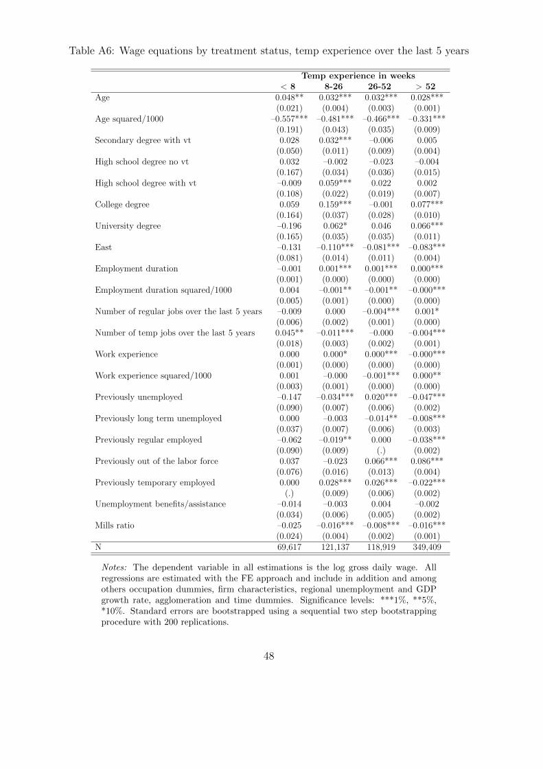
Table A6: Wage equations by treatment status, temp experience over the last 5 years

Temp experience in weeks< 8 8-26 26-52 > 52

Age 0.048** 0.032*** 0.032*** 0.028***(0.021) (0.004) (0.003) (0.001)

Age squared/1000 –0.557*** –0.481*** –0.466*** –0.331***(0.191) (0.043) (0.035) (0.009)

Secondary degree with vt 0.028 0.032*** –0.006 0.005(0.050) (0.011) (0.009) (0.004)

High school degree no vt 0.032 –0.002 –0.023 –0.004(0.167) (0.034) (0.036) (0.015)

High school degree with vt –0.009 0.059*** 0.022 0.002(0.108) (0.022) (0.019) (0.007)

College degree 0.059 0.159*** –0.001 0.077***(0.164) (0.037) (0.028) (0.010)

University degree –0.196 0.062* 0.046 0.066***(0.165) (0.035) (0.035) (0.011)

East –0.131 –0.110*** –0.081*** –0.083***(0.081) (0.014) (0.011) (0.004)

Employment duration –0.001 0.001*** 0.001*** 0.000***(0.001) (0.000) (0.000) (0.000)

Employment duration squared/1000 0.004 –0.001** –0.001** –0.000***(0.005) (0.001) (0.000) (0.000)

Number of regular jobs over the last 5 years –0.009 0.000 –0.004*** 0.001*(0.006) (0.002) (0.001) (0.000)

Number of temp jobs over the last 5 years 0.045** –0.011*** –0.000 –0.004***(0.018) (0.003) (0.002) (0.001)

Work experience 0.000 0.000* 0.000*** –0.000***(0.001) (0.000) (0.000) (0.000)

Work experience squared/1000 0.001 –0.000 –0.001*** 0.000**(0.003) (0.001) (0.000) (0.000)

Previously unemployed –0.147 –0.034*** 0.020*** –0.047***(0.090) (0.007) (0.006) (0.002)

Previously long term unemployed 0.000 –0.003 –0.014** –0.008***(0.037) (0.007) (0.006) (0.003)

Previously regular employed –0.062 –0.019** 0.000 –0.038***(0.090) (0.009) (.) (0.002)

Previously out of the labor force 0.037 –0.023 0.066*** 0.086***(0.076) (0.016) (0.013) (0.004)

Previously temporary employed 0.000 0.028*** 0.026*** –0.022***(.) (0.009) (0.006) (0.002)

Unemployment benefits/assistance –0.014 –0.003 0.004 –0.002(0.034) (0.006) (0.005) (0.002)

Mills ratio –0.025 –0.016*** –0.008*** –0.016***(0.024) (0.004) (0.002) (0.001)

N 69,617 121,137 118,919 349,409

Notes: The dependent variable in all estimations is the log gross daily wage. Allregressions are estimated with the FE approach and include in addition and amongothers occupation dummies, firm characteristics, regional unemployment and GDPgrowth rate, agglomeration and time dummies. Significance levels: ***1%, **5%,*10%. Standard errors are bootstrapped using a sequential two step bootstrappingprocedure with 200 replications.

48

Table A7: Wage equations by treatment status, number of temp jobs over the last 5 years

Number of temp jobs1 2 3 > 3

Age 0.036*** 0.030*** 0.017*** 0.019***(0.001) (0.001) (0.002) (0.003)

Age squared/1000 –0.426*** –0.361*** –0.197*** –0.284***(0.009) (0.016) (0.025) (0.029)

Secondary degree with vt –0.005 0.016* 0.038*** 0.017*(0.006) (0.008) (0.014) (0.010)

High school degree no vt 0.003 0.041 0.239*** 0.019(0.019) (0.027) (0.044) (0.047)

High school degree with vt –0.015 0.030** 0.022 0.026(0.011) (0.013) (0.021) (0.016)

College degree 0.022* 0.223*** –0.140*** 0.057**(0.013) (0.018) (0.040) (0.029)

University degree 0.079*** 0.229*** 0.118*** 0.030(0.014) (0.019) (0.042) (0.036)

East –0.115*** –0.092*** –0.116*** –0.062***(0.008) (0.008) (0.010) (0.008)

Employment duration 0.001*** 0.001*** 0.000*** 0.001***(0.000) (0.000) (0.000) (0.000)

Employment duration squared/1000 –0.002*** –0.001*** –0.001*** –0.002***(0.000) (0.000) (0.000) (0.000)

Number of regular jobs over the last 5 years –0.002*** –0.004*** –0.004*** 0.001**(0.000) (0.001) (0.001) (0.001)

Work experience 0.000*** 0.000*** 0.000*** 0.000(0.000) (0.000) (0.000) (0.000)

Work experience squared/1000 –0.001*** –0.001*** –0.002*** –0.001(0.000) (0.000) (0.000) (0.000)

Previously unemployed 0.003 0.025*** –0.075*** –0.023***(0.003) (0.005) (0.006) (0.005)

Previously long term unemployed –0.007** –0.030*** 0.002 –0.018**(0.004) (0.005) (0.008) (0.008)

Previously regular employed –0.001 0.000 –0.042*** –0.022***(0.002) (.) (0.008) (0.006)

Previously out of the labor force –0.011** –0.005 0.116*** 0.162***(0.005) (0.008) (0.013) (0.014)

Previously temporary employed 0.000 0.041*** –0.062*** –0.020***(.) (0.005) (0.006) (0.005)

Unemployment benefits/assistance –0.043*** –0.002 –0.004 –0.005(0.004) (0.005) (0.006) (0.004)

Mills ratio 0.000 –0.004*** 0.002 –0.002**(0.001) (0.001) (0.002) (0.001)

N 353,764 157,340 74,440 73,538

Notes: The dependent variable in all estimations is the log gross daily wage. Allregressions are estimated with the FE approach and include in addition and amongothers occupation dummies, firm characteristics, regional unemployment and GDPgrowth rate, agglomeration and time dummies. Significance levels: ***1%, **5%,*10%.Standard errors are bootstrapped using a sequential two step bootstrappingprocedure with 200 replications.

49

Documents

Does the Sector Experience Affect the Pay Gap for ...doku.iab.de/veranstaltungen/2011/ws_flex2011_jahn_pozzoli.pdf · Does the Sector Experience A ect the Pay Gap for Temporary Agency