Does Trade Liberalization with China Influence U.S. Elections? · PDF fileYi Che, Yi Lu, Justin R. Pierce, Peter K. Schott, and Zhigang Tao 2016-039 Please cite this paper as: Che,

Finance and Economics Discussion SeriesDivisions of Research & Statistics and Monetary Affairs

Federal Reserve Board, Washington, D.C.

Does Trade Liberalization with China Influence U.S. Elections?

Yi Che, Yi Lu, Justin R. Pierce, Peter K. Schott, and Zhigang Tao

2016-039

Please cite this paper as:Che, Yi, Yi Lu, Justin R. Pierce, Peter K. Schott, and Zhigang Tao (2016). “DoesTrade Liberalization with China Influence U.S. Elections?,” Finance and Economics Dis-cussion Series 2016-039. Washington: Board of Governors of the Federal Reserve System,http://dx.doi.org/10.17016/FEDS.2016.039.

NOTE: Staff working papers in the Finance and Economics Discussion Series (FEDS) are preliminarymaterials circulated to stimulate discussion and critical comment. The analysis and conclusions set forthare those of the authors and do not indicate concurrence by other members of the research staff or theBoard of Governors. References in publications to the Finance and Economics Discussion Series (other thanacknowledgement) should be cleared with the author(s) to protect the tentative character of these papers.

Does Trade Liberalization with China In�uence U.S.

Elections?∗

Yi Che†

Shanghai Jiao Tong University

Yi Lu‡

National University of Singapore

Justin R. Pierce§

Board of Governors of the Federal Reserve System

Peter K. Schott¶

Yale School of Management & NBER

Zhigang Tao‖

University of Hong Kong

First Draft: September 2015This Draft: April 2016

Abstract

This paper examines the impact of trade liberalization on U.S. Congressional

elections. We �nd that U.S. counties subject to greater competition from China

via a change in U.S. trade policy exhibit relative increases in turnout, the share

of votes cast for Democrats and the probability that the county is represented by

a Democrat. We �nd that these changes are consistent with Democrats in o�ce

during the period examined being more likely than Republicans to support legis-

lation limiting import competition or favoring economic assistance. (JEL Codes:

F13; F16; D72) (Keywords: China; Voting; Elections; Import Competition; Nor-

mal Trade Relations; World Trade Organization)

∗We thank participants at the 2015 NBER China meeting for helpful comments. Any opinions andconclusions expressed herein are those of the authors and do not necessarily represent the views ofthe Board of Governors or its research sta�.†[email protected]‡[email protected]§[email protected].¶[email protected].‖[email protected]

1

1 Introduction

International trade has long been a contentious issue in U.S. elections. During the2000s, the U.S. trade de�cit with China emerged as a focus of particular attention,and recent research establishes a link between growing U.S. imports from China andthe sharp loss of U.S. manufacturing jobs after the year 2000. Autor et al. (2013), forexample, �nd that 25 to 50 percent of the manufacturing job loss in the United Statesbetween 2000 and 2007 is due to rising Chinese imports, while Pierce and Schott (2016)show that this relationship is associated with a change in U.S. trade policy � the U.S.granting of permanent normal trade relations (PNTR) to China � which eliminatedthe threat of substantial tari� increases on Chinese imports. This heightened exposureto Chinese import competition may a�ect voters' preferences through several channels,including employment, wages, pro�ts and goods prices.

This paper examines the impact of increased exposure to competition from China onelections for the U.S. House of Representatives as well as the legislative activity of thoseelected to Congress. In the �rst part of our analysis, we show that U.S. counties withgreater exposure to the change in U.S. trade policy exhibit larger increases in turnoutas well as the share of votes cast for Democrats and the probability that a Democratrepresents the county. The second part of our analysis documents a rationale for thischange in voting behavior by showing that Congressional Democrats are, in fact, morelikely to support policies that place restrictions on imports and that provide economicassistance that might mitigate the impact of import competition.

Our measure of exposure to increased competition from China arises from the U.S.granting of PNTR to China in October 2000. Prior to this change in U.S. trade policy,U.S. imports from China faced the risk, each year, that tari�s on a subset of productswould rise from the low NTR tari� rates o�ered to WTO members to the substantiallyhigher non-NTR rates set in the Smoot-Hawley Tari� Act of 1930. These potentialtari� increases created a disincentive for U.S. �rms to take advantage of productionin China and for Chinese �rms to expand into the U.S. market. By eliminating thepossibility of these future tari� increases, PNTR removed these disincentives.

We examine voting in elections for the U.S. House of Representatives because Housemembers serve two-year terms and are expected to maintain close personal contact withconstituents. As a result, House members may be more responsive to the demands ofvoters than elected o�cials with longer terms such as Senators or Presidents.1 Weexamine voting at the county rather than Congressional district level in order to trackchanges within constant geographic areas over time. That approach is not possible atthe district level because the borders of Congressional districts change substantiallyduring the period we examine (1992 to 2010) as a result of redistricting after the 2000

1Karol (2012) �nds that Senators and Presidents are more likely to support policies (like free trade)that are in the long-run interests of the country as a whole, even if they run counter to the short-run passions of voters. Conconi et al. (2014) show that Senators are more likely to support tradeliberalization than Representatives, but that the result does not hold for Senators facing electionswithin the next two years.

2

Census. County borders, by contrast, are stable over this period. One potential ad-ditional bene�t of focusing on counties is that they are smaller than Congressionaldistricts in terms of both area and population, allowing us to capture greater variationin both exposure to Chinese import competition and residents' demographic charac-teristics.

Our di�erence-in-di�erences empirical strategy examines whether counties moreexposed to the change in U.S. policy (�rst di�erence) experience di�erential changesin voting for Democrats after the policy is implemented (second di�erence). Acrossspeci�cations that are either unweighted or weighted by counties' initial population,coe�cient estimates suggest that moving a county from the 25th to the 75th percentilein terms of exposure to the change in U.S. trade policy is associated with a 1 to 2percentage point increase in the share of votes cast for Democrats, representing a 3 to4 percent increase relative to the across-county average share of votes for Democratsin the 2000 Congressional election, the closest Congressional election to the change inU.S. trade policy. Coe�cient estimates from similar speci�cations indicate that theprobability of a switch in representation for a county from a Republican to a DemocratRepresentative increases by 2 to 3 percentage points.

We allow for the potential in�uence of spillovers from nearby areas by controllingfor changes in exposure to China experienced by neighboring counties that are part ofthe same labor market. Results from these speci�cations are qualitatively similar tothe baseline speci�cations but somewhat larger in magnitude: moving a county fromthe 25th to the 75th percentile in terms of both own exposure to the policy change andneighboring counties' exposure is associated with a 4.4 percent increase in the share ofvotes won by the Democrat relative to the average share of votes won by Democratsin the year 2000 election, versus 3.7 percent in the baseline speci�cation.

We also document other related evidence supportive of a role for PNTR in U.S. elec-tion outcomes. First, we �nd that the increase in the share of votes cast for Democratsassociated with PNTR is also present for Presidential and Gubernatorial elections,indicating e�ects for electoral contests besides the U.S. House of Representatives. Sec-ond, we �nd that counties more exposed to PNTR's trade liberalization exhibit largerincreases in voter turnout after the policy change, relating to the political science liter-ature on the e�ect of economic conditions on voter turnout (e.g. Schlozman and Verba1979).

The second part of our analysis examines Representatives' Congressional votes onlegislation during the 1990s and 2000s using a regression discontinuity identi�cationstrategy that compares the voting of Democrats and Republicans who win o�ce bysmall margins. The analysis indicates that Democrats during this period are morelikely to take positions that restrict trade and that o�er economic assistance that maybene�t those adversely a�ected by trade, providing a rationale for the change in votingdocumented in the �rst part of the paper. We �nd that the tendency for Democratsto support such legislation is stronger after implementation of PNTR.

Together, the results in the �rst and second parts of the paper suggest that voterswho perceive themselves as being disadvantaged by trade are more likely to vote for

3

politicians that might restrict imports. An interesting topic for future research is theextent to which PNTR contributes to the strong performance of candidates proposingto restrict trade or alter trade agreements among both Republicans and Democratsduring the 2016 Presidential primaries.

This paper relates to literatures on voting in both political science and economics,and also complements the large literature examining the impact of international tradeon worker outcomes.2 A closely related paper in the voting literature is Feigenbaumand Hall (2015), which examines the e�ect of Congressional-district-level economicshocks from Chinese imports � using the approach in Autor, Dorn and Hanson (2013)� on the roll-call behavior of legislators and electoral outcomes. They �nd that legisla-tors from districts experiencing larger increases in Chinese import competition becomemore protectionist in their voting on trade-related bills, and that incumbents are ableto insulate themselves from electoral competition via this voting behavior. Anotherclosely related paper is Jensen, Quinn and Weymouth (2016), which �nds that votesfor presidential candidates' incumbent parties rise with expanding U.S. exports andfall with rising U.S. imports.

Using data from German labor markets, Dippel, Gold and Heblich (2015) �nd thathigher imports from Eastern Europe and China are associated with an increase in theshare of votes for far right parties.3 And in research examining the relationship betweenimmigration and elections, Mayda, Peri and Steingress (2016) �nd that the share ofvotes cast for Republicans in U.S. elections responds to the level of immigration, withthe e�ect varying based on the share of naturalized migrants and non-citizen migrantsin the population.

This paper also relates to a literature that examines the role of trade on legisla-tors' voting activity. Conconi et al. (2012) examine the impact of district-level tradecompetition on Representatives' votes to grant U.S. Presidents Fast Track Authorityvis a vis the negotiation of trade agreements, and Conconi et al. (2015) examine therole of skilled labor abundance in Representatives' votes on trade and immigrationbills. Blonigen and Figlio (1998) �nd that legislators' votes for bills related to tradeprotection are positively associated with direct foreign investment.

We proceed as follows. Section 2 provides an overview of the growth of U.S.-Chinatrade. Section 3 describes our data sources. Sections 4 and 5 present our empiricalresults. Section 6 concludes.

2A substantial body of research documents a negative relationship between import competitionand U.S. manufacturing employment, e.g., Freeman and Katz (1991), Revenga (1992), Sachs andShatz (1994) and Bernard et al. (2006). More recently, a series of papers link Chinese imports toemployment outcomes in the United States and other developed or developing countries, e.g., Autoret al. (2013), Bloom et al. (2015), Ebenstein et al. (2014), Groizard, Ranjan and Rodriguez-Lopez(2012), Mion and Zhu (2013) and Utar and Torres Ruiz (2013). Increasingly active areas of researchexamine links between international trade and health (McManus and Schaur 2015a,b and Pierce andSchott 2016), crime (Dix-Carneiro et al. 2015 and Che and Xu 2015), and the provision of publicgoods, (Feler and Senses 2015 and Che and Xu 2015).

3Scheve and Slaughter (2001) show that individuals' trade policy preferences are a�ected by skilllevel and homeownership status.

4

2 China's Growth as a U.S. Trade Partner

In the past thirty-�ve years China jumped from being an insigni�cant contributor toworld GDP to the world's second-largest economy and largest trading state. In 2007it became the United States' largest source of imports, accounting for 17 percent of allimports versus just 3 percent in 1990. As illustrated in Figure 1, U.S. imports fromChina accelerated after China's receipt of PNTR in 2000. U.S. exports to China alsogrew substantially over this period, but less rapidly, with the result that by 2007 theUnited States trade de�cit with China exceeded $250 billion U.S. dollars, or 1.7 percentof GDP, up from 0.3 percent of GDP in 1990.

As illustrated in Figure 2, the United States' growing imports from China coincidewith a sharp, 18 percent decline in U.S. manufacturing employment from 2001 to 2007,with more than 80 percent of the decline occurring between 2001 and 2004. Pierceand Schott (2016) show that this decline was steeper in industries more exposed to theU.S. granting of permanent normal trade relations to China, while Autor et al. (2013)show that commuting zones with industrial structures more similar to U.S. importsfrom China experienced greater declines in manufacturing employment. Beyond man-ufacturing employment, Pierce and Schott (2015) show that counties more exposed toPNTR experience both relatively higher levels of unemployment and lower levels oflabor force participation during the 2000s. Related adjustment costs for workers whoswitch industries or occupations as a result of these trends, and which might be in�u-ential in driving voting preferences, are highlighted in Artuc et al. (2010), Ebensteinet al. (2014), Acemoglu et al. (2013) and Caliendo et al. (2015).

Growth in the U.S. trade de�cit with China has motivated U.S. legislators at var-ious levels of government to propose restricting imports from China. As discussed inPierce and Schott (2016), Congress demonstrated substantial resistance to the renewalof normal trade relations for China during the 1990s. Then, after the extension ofPNTR and China's entry into the WTO in 2001, Senators Charles Schumer and Lind-sey Graham repeatedly introduced legislation in the U.S. Senate to impose tari�s onU.S. imports from China based on allegations that China manipulates its exchange raterelative to the U.S. dollar (Lichtblau 2011). Calls for such action generally increaseduring elections. Indeed, in a move the New York Times referred to as �election yearpolitics over a loss of American jobs� (Sanger and Chan 2010), the House of Repre-sentatives in 2010 granted President Obama expanded authority to impose tari�s ona wide range of Chinese goods. The 2012 Presidential election and the lead-up to the2016 election have also featured sharp dialogue relating to trade with China from bothRepublicans and Democrats.4

4For example, Donald Trump has called for a 45 percent tari� on U.S. imports from China(Haberman 2016) and Bernie Sanders proposes �Reversing trade policies like NAFTA, CAFTAand PNTR with China that have driven down wages and caused the loss of millions of jobs�(www.berniesanders.com/issues/income-and-wealth-inequality/). Recent media coverage has focusedon the role of these trade positions in support for Trump and Sanders, e.g. Stromberg (2016). Foradditional examples, see Brower and Lerer (2012) for the 2012 election, and Collinson (2015) for the

5

3 Data

This section describes the data used to measure election outcomes, exposure to compe-tition from China, and other trade-related variables that may a�ect election outcomes.

3.1 Election Results and Demographics

Data on county-level election outcomes from 1992 to 2010 are from Dave Leip's Atlas

of U.S. Presidential Elections.5 These data track the number of votes received byDemocratic and Republican candidates for Congress in each county in each electionyear, as well as the number of registered voters.6

Figure 3 reports the distribution of the Democrat vote share across counties overthe sample period. As indicated in the �gure, the average county experienced a declinein Democrat vote share during the 1990s and early 2000s, followed by a rebound in2006 and 2008, and then a decline in 2010. The mean Democrat vote share in the 2000Congressional election is 40 percent, with a standard deviation of 23 percentage points.

We match the voting data to county-level demographic data from the 1990 Decen-nial Census that have been found to be important correlates of voting behavior in thepolitical science and economics literatures on voting.7 These data are summarized inTable 1.

3.2 Counties' Exposure to PNTR

We make use of the structure of the U.S. tari� schedule to de�ne a measure of eachindustry's � and in turn, each county's � exposure to PNTR. The tari� schedule hastwo basic sets of tari�s: NTR tari�s, which average 4 percent across industries andare applied to goods imported from other members of the World Trade Organization(WTO); and non-NTR tari�s, which were set by the Smoot-Hawley Tari� Act of 1930and are typically substantially higher than the corresponding NTR rates, averaging 37percent across industries. While imports from non-market economies, such as China,generally are subject to the higher non-NTR rates, U.S. tari� law allows the Presidentto grant such countries access to NTR rates on an annually renewable basis, subjectto approval by Congress.

2016 election cycle.5For details on data collection, see www.uselectionatlas.org.6County boundaries are substantially more stable than those of Congressional districts, whose

borders change after each decennial census During our sample period, there are only three changes:South Boston, VA (county code 51780) joined Halifax County (51083) on July 1, 1995; Dade County,FL (12025) was renamed as Miami-Dade FL (12086) on November 13, 1997; and Skagway-Yakutat-Angoon, AK (2231) was changed to Skagway-Hoonah-Angoon Census Area, AK (2232) on September22, 1992, and then to Hoonah-Angoon Census Area, AK on June 20, 2007. In each case, we aggregatethe noted counties for the entire sample period.

7See, for example, Baldwin and Magee (2000), Gilbert and Oladi (2012), Kriner and Reeves (2012),Wright (2012) and Conconi et al. (2012).

6

U.S. Presidents granted China such a waiver every year starting in 1980, but annualre-approval of the waiver became politically contentious following the Chinese govern-ment's crackdown on the Tiananmen Square protests in 1989. Re-approval remainedcontroversial throughout the 1990s, especially during other �ashpoints in U.S.-Chinarelations including China's transfer of missile technology to Pakistan in 1993 and theTaiwan Straits Missile Crisis in 1996. Importantly, if annual renewal of the waiver hadfailed, U.S. tari�s on imports from China generally would have risen substantially fromthe temporary NTR level to the much higher non-NTR rates.

The possibility of tari� increases each year served as a disincentive for �rms con-sidering engaging in U.S.-China trade.8 Pierce and Schott (2016) provide anecdotesindicating that this threat both discouraged U.S. �rms from making investments inChina and suppressed investments by Chinese �rms considering exporting to the UnitedStates, thereby reducing import competition for U.S. producers.

PNTR, which was passed by Congress in October 2000 and took e�ect upon China'sentry to the WTO in December 2001, permanently locked in U.S. tari�s on importsfrom China at the low NTR rates, eliminating these disincentives.9 As documentedin Pierce and Schott (2016), the industries and products most a�ected by the policychange experienced larger declines in U.S. manufacturing employment, as well as largerincreases in imports from China � including related-party imports � and larger increasesin exports to the United States by foreign-owned �rms in China.10

We compute counties' exposure to PNTR in two steps. The �rst step is to calcu-late exposure for U.S. industries. We follow Pierce and Schott (2016) in de�ning theindustry-level impact of PNTR as the increase in U.S. tari�s on Chinese goods thatwould have occurred in the event of a failed annual renewal of China's NTR statusprior to PNTR,

NTR Gapj = Non NTR Ratej −NTR Ratej. (1)

We refer to this di�erence as the NTR gap, and compute it for each four-digit SICindustry j using ad valorem equivalent tari� rates provided by Feenstra et al (2002)for 1999, the year before passage of PNTR. As illustrated in Figure 4, NTR gaps varywidely across industries, with a mean and standard deviation of 33 and 15 percentagepoints, respectively. As noted in Pierce and Schott (2016), 79 percent of the variationin the NTR gap across industries is due to non-NTR rates, set 70 years prior to passage

8Intuition for these incentives can be derived, in part, from the literature on investment underuncertainty (e.g., Pindyck 1993 and Bloom, Bond and Van Reenen 2007), which demonstrates that�rms are more likely to undertake irreversible investments as the ambiguity surrounding their expectedpro�t decreases. Handley (2014) introduces these insights to �rms' decisions to export.

9The passage of PNTR followed the bilateral agreement in 1999 between the U.S. and Chinaregarding China's eventual entry into the WTO.

10Feng, Li and Swenson (2016) discuss the e�ect of PNTR on entry and exit patterns of Chineseexporters, as well as changes in export product characteristics; Heise et al. (2015) describe the e�ectof PNTR on the structure of supply chains; and Handley and Limao (2014) discuss its implicationsfor trade.

7

of PNTR. This feature of non-NTR rates e�ectively rules out reverse causality thatwould arise if non-NTR rates were set to protect industries with declining employmentor surging imports. Furthermore, to the extent that NTR rates were raised to protectindustries with declining employment prior to PNTR, these higher NTR rates wouldresult in lower NTR gaps, biasing our results away from �nding an e�ect of PNTR.11

We compute U.S. counties' exposure to PNTR as the employment-share weightedaverage NTR gap across the sectors in which they are active,

NTR Gapc =∑

j

(Ljcb

Lcb

NTR Gapj

), (2)

where Ljcb is the base-year b employment of SIC industry j in county c and Lcb is theoverall employment in county c in base year b.12

County-industry-year employment data are from the U.S. Census Bureau's CountyBusiness Patterns (CBP). We use b = 1990 for the base year to mitigate a potentialrelationship between counties' industrial structure and the year 2000 change in U.S.trade policy. Given that services comprise a large share of employment, the distri-bution of county-level NTR Gapc is shifted leftwards relative to the distribution ofmanufacturing and other industries for which the NTRGapj is de�ned: the mean andstandard deviation of the county-level NTR gap are 7.3 and 6.5 percentage points, asdisplayed visually in Figure 5. The di�erence between the 25th and 75th percentiles is8.3 (=10.6-2.3) percentage points.

We also compute counties' exposure to PNTR via the average NTR gap of sur-rounding counties in the same commuting zone, a geographic area roughly analogousto a local labor market.13 The correlation of own- and commuting-zone NTR gapsacross counties, 0.58, is displayed visually in Figure 6.

3.3 Other Controls for Exposure to Import Competition

Our analysis includes controls for counties' average NTR rate and their exposure to thephasing out of textile and clothing quotas under the global Multi-Fiber Arrangement(Khandelwal et al. 2013).

We compute counties' exposure to U.S. import tari�s and the MFA phase-outs asthe employment-share weighted average of their tari� rates and exposure to MFA, i.e.,as in equation 2. Following Brambilla et al. (2009) and Pierce and Schott (2016),

11Cross-industry variation in the NTR rate explains less than 1 percent of variation in the NTRgap.

12NTR gaps can only be calculated for products subject to import tari�s, such as manufacturing,agriculture and mining products. NTR gaps for services, which are not subject to import tari�s are,by de�nition, zero.

13We use the U.S. Census Bureau de�nition of commuting zones as of 1990 and the concordance ofcounties to commuting zones provided by Autor et al. (2013). The 3113 counties in our sample aredistributed across 741 commuting zones, with the number of counties per commuting zone rangingfrom 1 to 19 (the Washington DC area).

8

we measure the extent to which industry quotas were binding under the MFA as theimport-weighted average �ll rate of the textile and clothing products that were underquota in that industry, where �ll rates are de�ned as the actual imports divided byallowable imports under the the quota. Industries with higher average �ll rates facedmore binding quotas and are therefore more exposed to the end of the MFA. Productsnot covered by the MFA have a �ll rate of zero.

4 Trade Liberalization with China and Voting in U.S.

Congressional Elections

This section explores the link between the U.S. granting of PNTR to China in 2000and outcomes of U.S. Congressional elections.

4.1 Identi�cation Strategy

Our baseline estimation examines the link between the share of votes cast for theDemocratic candidate for the U.S. House of Representatives in county c in even electionyear t from 1992 to 2010, a period that straddles the year 2000 change in U.S. tradepolicy. We use a di�erence-in-di�erences (DID) speci�cation that asks whether countieswith higher NTR gaps (�rst di�erence) experience di�erential changes in voting afterthe change in U.S. trade policy (second di�erence),

DemV otect = θPost PNTRt × NTRGapc (3)

+Post PNTRt×X′cγ +X′ctβ

+δc + δt + α + εct,

The dependent variable is the percent of votes received by the Democrat in county c inyear t. The �rst term on the right-hand side is the DID term of interest, an interactionof a post-PNTR (i.e., t > 2000) indicator with the (time-invariant) county-level NTRgap, as de�ned in the preceding section.

Xc represents a vector of initial period county demographic attributes taken fromthe 1990 Census that are found to be important in the economics and political sci-ence literatures on voting. These attributes are median household income, share ofpopulation achieving higher education, the share of non-white population, the shareof veterans and the share of voters over 65. Including interactions of these attributeswith the Post PNTRt indicator allows the relationship between these demographiccharacteristics and voting outcomes to di�er before and after passage of PNTR. Xct

represents a matrix of time-varying policy attributes including the average U.S. importtari� rate associated with each county's mix of industries as well as the county's expo-sure to the phasing out of the MFA. δc and δt represent county and year �xed e�ects.

9

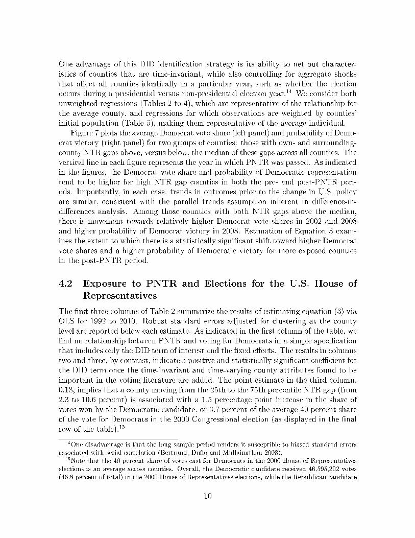
One advantage of this DID identi�cation strategy is its ability to net out character-istics of counties that are time-invariant, while also controlling for aggregate shocksthat a�ect all counties identically in a particular year, such as whether the electionoccurs during a presidential versus non-presidential election year.14 We consider bothunweighted regressions (Tables 2 to 4), which are representative of the relationship forthe average county, and regressions for which observations are weighted by counties'initial population (Table 5), making them representative of the average individual.

Figure 7 plots the average Democrat vote share (left panel) and probability of Demo-crat victory (right panel) for two groups of counties: those with own- and surrounding-county NTR gaps above, versus below, the median of these gaps across all counties. Thevertical line in each �gure represents the year in which PNTR was passed. As indicatedin the �gures, the Democrat vote share and probability of Democratic representationtend to be higher for high NTR gap counties in both the pre- and post-PNTR peri-ods. Importantly, in each case, trends in outcomes prior to the change in U.S. policyare similar, consistent with the parallel trends assumption inherent in di�erence-in-di�erences analysis. Among those counties with both NTR gaps above the median,there is movement towards relatively higher Democrat vote shares in 2002 and 2008and higher probability of Democrat victory in 2008. Estimation of Equation 3 exam-ines the extent to which there is a statistically signi�cant shift toward higher Democratvote shares and a higher probability of Democratic victory for more exposed countiesin the post-PNTR period.

4.2 Exposure to PNTR and Elections for the U.S. House of

Representatives

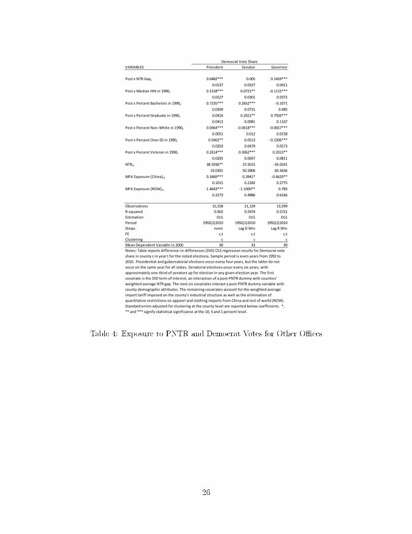
The �rst three columns of Table 2 summarize the results of estimating equation (3) viaOLS for 1992 to 2010. Robust standard errors adjusted for clustering at the countylevel are reported below each estimate. As indicated in the �rst column of the table, we�nd no relationship between PNTR and voting for Democrats in a simple speci�cationthat includes only the DID term of interest and the �xed e�ects. The results in columnstwo and three, by contrast, indicate a positive and statistically signi�cant coe�cient forthe DID term once the time-invariant and time-varying county attributes found to beimportant in the voting literature are added. The point estimate in the third column,0.18, implies that a county moving from the 25th to the 75th percentile NTR gap (from2.3 to 10.6 percent) is associated with a 1.5 percentage point increase in the share ofvotes won by the Democratic candidate, or 3.7 percent of the average 40 percent shareof the vote for Democrats in the 2000 Congressional election (as displayed in the �nalrow of the table).15

14One disadvantage is that the long sample period renders it susceptible to biased standard errorsassociated with serial correlation (Bertrand, Du�o and Mullainathan 2003).

15Note that the 40 percent share of votes cast for Democrats in the 2000 House of Representativeselections is an average across counties. Overall, the Democratic candidate received 46,595,202 votes(46.8 percent of total) in the 2000 House of Representatives elections, while the Republican candidate

10

Columns four through six of Table 2 examine the relationship between PNTR andthree other election outcomes: an indicator variable for whether the Democrat winsthe county, an indicator for whether the election results in a switch to a Democratrepresenting the county, and an indicator for whether the election results in a switchto a Republican representing the county.16 For the latter two regressions the sampleis restricted to observations in which the prior o�ce holder was a Republican, orDemocrat, respectively.

As indicated in the table, we �nd a positive and statistically signi�cant relationshipbetween exposure to PNTR and the probability of both Democrat victory and a switchto a Democratic Representative. By contrast, we �nd a statistically signi�cant declinein the probability of a switch to a Republican Representative. The point estimate forDemocrat victory in column four, 0.2282, indicates that a county moving from the25th to the 75th percentile NTR gap is associated with a 1.9 percentage point increasein the probability of victory, or 5.4 percent of the probability of victory in the year2000. Similar exercises indicate an estimated increase in the probability of switchingto Democrat of 1.9 percentage points, and an estimated decrease in the probability ofswitching to a Republican of -2.2 percentage points. These estimated changes representapproximately 27 and -17 percent of the average probabilities of such switches occurringin the year 2000 (7 and 13 percent, respectively).

Estimates for the remaining covariates included in the regression suggest that voterswith a college degree and at least some graduate education are more likely to supportDemocrats after 2000, while those over 65 are less likely to do so.

The �nal column of Table 2 examines the relationship between exposure to PNTRand voter turnout, de�ned as the number of people voting in the election divided by thenumber of registered voters.17 As indicated in the table, we �nd that higher exposureto PNTR is associated with a statistically and economically signi�cant increase invoter turnout. The point estimate for the DID term, 0.14, suggests that a countymoving from the 25th to the 75th percentile in terms of exposure is associated with a1.18 percentage point increase in turnout, or 1.8 percent of the average turnout acrosscounties in the year 2000 (65 percent).

To the extent that the median voter is injured by increased import competition inthe more heavily-a�ected counties, this result is in line with a political science literaturearguing that economic adversity can increase voter turnout (e.g. Schlozman and Verba1979). This result di�ers from Dippel, Gold and Heblich's (2015) �nding that higherimports have no relationship with election turnout in Germany. The di�erence maystem, in part, from U.S. voters directing votes toward a major party in response to trade

received 46,738,619 votes (47.0 percent of total) and candidates from other parties received 6,125,773votes (6.2 percent of total). See Federal Election Commission (2001).

16Because counties are reallocated to Congressional districts over time, we emphasize that thisanalysis does not directly examine victories in House elections, but rather examines the probabilitythat a Representative from a particular party represents a county.

17Turnout data are missing from Dave Leip's Atlas of U.S. Presidential Elections for 1992, 1994,1998 and 2008.

11

competition, whereas Dippel, Gold and Heblich (2015) show that import competitionin Germany is associated with an increase in votes for far-right parties.

4.3 Exposure to PNTR via Neighboring Counties Within Com-

muting Zones

In this section we examine whether voters in one county might be in�uenced by eco-nomic conditions in neighboring counties that are part of the same labor market. Thespeci�cation we consider is similar to that considered in the previous section but itis augmented with an additional di�erence-in-di�erences term, an interaction of thepost-PNTR indicator variable with the average NTR gap across other counties in thesame commuting zone (z).

As illustrated in Table 3, the estimated coe�cients for both own and externalcommuting zone NTR gaps are positive for all �ve outcome variables: the Democratvote share, the probability of Democrat victory, the probability of a switch towardsa Democrat or away from a Republican, and turnout. Though estimates for the twoDID terms are not individually signi�cant, they are jointly signi�cant in all cases, asindicated by the F-test p-values reported in the third-to-last row of the table.

In terms of economic signi�cance, the coe�cient estimates in the �rst column sug-gest that a county moving from the 25th to the 75th percentile NTR gap (from 2.3 to10.6 percent) is associated with a 1.8 percentage point increase in the share of voteswon by the Democrat candidate, representing 4.4 percent of the average 40 percentshare of the vote for Democrats in the year 2000. Point estimates in the third columnindicate that moving a county from the 25th to the 75th percentile NTR gap boosts theprobability or Democrat victory by 6.3 percent compared to the average probabilityof victory across counties in the year 2000. For switching to a Democrat, switching toa Republican and turnout, the comparable percentages are 28, -32 and 1.25 percent,respectively. These magnitudes are all somewhat larger than those reported in thebaseline results indicating that counties' voting outcomes are also a�ected by spilloversfrom neighboring counties in the same labor market.

4.4 Exposure to PNTR and the Democrat Vote Share for Other

O�ces

In this section we examine the relationship between PNTR and the Democrat voteshare for three other o�ces: Presidential, Senatorial and gubernatorial. Presidentialand gubernatorial elections occur every four years, but unlike Presidential elections,the latter do not all occur in the same year for all states. Senatorial elections occurevery six years, with approximately one third of Senators up for election in any givenelection year.

Results are reported in Table 5. We �nd positive and statistically signi�cant re-lationships between the change in U.S. trade policy and the share of votes won by

12

Democrats in both Presidential and gubernatorial elections. The DID point estimatesfor President and governor suggest that moving a county from the 25th to the 75thpercentile in terms of exposure to PNTR is associated with increases in the Democratvote share of 0.4 and 1.2 percentage points, or 1 and 2.5 percent of the average shareof votes won by Democrats for these o�ces across counties in the year 2000. We also�nd a positive relationship between PNTR and the share of votes won by Democrats inSenatorial elections, but this relationship is not statistically signi�cant at conventionallevels. The observed e�ects on Presidential and gubernatorial outcomes provide furtherevidence consistent with the role of PNTR's trade liberalization on elections.

4.5 Weighting Counties by Population

The coe�cient estimates reported in the previous three sections are based on un-weighted regressions, and therefore are representative of the relationship between PNTRand voting behavior for the average county. In this section we consider the e�ect ofweighting by initial (1990) population, which provides estimates representative of theaverage individual.

As indicated in Table 2, we continue to �nd positive and statistically signi�cant re-lationships between PNTR and the share of votes won by Democrats, the likelihood ofa switch to a Democrat Representative and turnout. We no longer �nd statistically sig-ni�cant relationships between counties' exposure to the change in U.S. trade policy andthe likelihood of either Democrat victory or a switch to a Republican Representative.

The point estimates in the �rst, third and �fth columns indicate that moving acounty from the 25th to the 75th percentile NTR gap increases the Democrat voteshare, the probability of a switch to a Democrat Representative and turnout by 2.8,18.9 and 3.3 percent relative to their levels in the year 2000. The �rst two of thesemagnitudes are somewhat lower than those implied by the estimates in Table 3 (3.7and 27, respectively), while the estimated e�ect for turnout is higher (1.8 in Table 3).

5 Party A�liation and Legislator Voting Behavior

The previous section establishes that voters in counties facing larger increases in compe-tition from China are more likely to vote for Democratic candidates. One explanationfor this result is that workers displaced by Chinese imports sought to elect o�cialsthat would either protect U.S. workers from international trade or soften the e�ectof this competition by promoting economic assistance programs. This section investi-gates whether Congressional Democrats in the U.S. House of Representatives duringthe 1990s and 2000s were more likely to vote for legislation along these lines. We usea regression discontinuity approach to examine whether Republicans' and Democrats'votes di�er on trade-related and economic assistance-related bills. We begin by dis-cussing the classi�cation of bills as being either for or against free trade or economicassistance and then describe our identi�cation strategy before presenting the results.

13

5.1 Classi�cation of �Trade� and �Economic Assistance� Bills

House members' votes from 1993 to 2011 (from the start of the 103rd to part of the112th Congresses) are obtained from the website www.govtrack.us. Data on the setof bills considered by the House during this period are from the Rohde/PIPC HouseRoll Call Database, maintained and generously provided by David Rohde of DukeUniversity. We adopt Rohde's classi�cations of bills related to trade and economicassistance programs, and then classify bills as pro- versus anti-free trade and pro-versus anti- economic assistance using ranking data from the National Journal. Wedescribe each of these steps in turn.

5.1.1 Trade Bills

The Rohde/PIPC House Roll Call Database assigns each bill a code summarizing itscontent.18 We follow Rohde in considering bills to be trade-related if they fall into thefollowing categories: �Japanese trade� (540), �Federal trade commission� (542), �un-fair trading practices� (543), �export controls� (544), �compensation to U.S. businessand workers� (545), �Export-Import Bank� (546), �tari� negotiations� (547), �importquotas-tari�s� (548), and �miscellaneous� (549). We classify trade-related bills as pro-versus anti-free trade based on the National Journal's rankings of the �economic liberal-ness� of the bills' sponsors.19 A ranking of rε(0, 100) indicates that the sponsor is more�liberal� in their voting than r percent of House members. Bills whose primary spon-sor's ranking exceeds 50 are coded as anti-free-trade. The remaining bills are coded aspro-free-trade. One drawback of this approach is its reliance on a ranking system basedexclusively on a principle component analysis of members' votes on economic issues.A major bene�t of the approach, in addition to its simplicity, is the independence ofthe rankings. We note that the results discussed below are also robust to the authors'qualitative classi�cation of bills as either pro- or anti-free trade.

5.1.2 Economic Assistance Bills

We consider bills to be related to economic assistance if they fall into the followingcategories of the Rohde database: �jobs� (code 810 of the database), �welfare bene-�ts/social services� (code 811), �job training� (code 816), �nutrition programs� (code831), �family assistance� (code 832), �homeless� (code 835), �unemployment assistance�(code 962), and �minimum wage� (code 966). As above, we use the National Journalrankings to classify bills as pro- versus anti- economic assistance according to whetherthe bills' sponsors' economic liberalness rankings are above or below 50.

18The complete list of codes can be found at http://sites.duke.edu/pipc/data/.19Further detail on these rankings is available at http://www.nationaljournal.com/2013-vote-

ratings/how-the-vote-ratings-are-calculated-20140206.

14

5.2 Identi�cation Strategy

We examine the relationship between House members' votes on trade and economicassistance bills and their party a�liation using the following speci�cation,

ydh = α + βDemocratdh +X′

dhθ + δs + δh + εdh, (4)

where d and h denote Congressional districts and the particular two-year Congressduring which Representatives serve.20 The dependent variable ydh represents the shareof anti-free trade or pro-economic assistance bills supported by a particular represen-tative during a particular Congress. The dummy variable Democratdh takes the value1 if the Representative is a Democrat and zero otherwise. Xdh represents a matrix ofdistrict-Congress attributes, including the demographic characteristics of the districtand personal attributes of the Representative.21 δs and δh represent state and Congress�xed e�ects, and εdh is the error term. As noted in the introduction, Congressional dis-trict boundaries change substantially over the sample period as a result of redistricting.We are therefore unable to include district �xed e�ects in equation 4.

In this speci�cation, identi�cation of β requires that Representatives' party a�l-iation be uncorrelated with the error term. As there may be several reasons whythis assumption is violated, we follow Lee (2008) in identifying the causal e�ect ofparty a�liation on voting behavior using a regression discontinuity (RD) approach.22

Speci�cally, we make use of the principle that the probability of a Democrat winninga congressional election disproportionately increases at the point where they receive alarger share of votes than the Republican competitor.

Formally, de�ne the assignment variable

Margindh ≡ V oteShareDemocraticdh − V oteSharesRepublican

dh

as the di�erence in voting share between the Democratic and Republican candidates inthe Congressional district d for election to Congress h. As illustrated in Figure 8, theprobability of a Democratic candidate winning an election conditional on the marginof victory has a discontinuity at the cuto� 0. That is, this probability is substantiallynear 1 for values of m just above zero compared with values of m just below zero.23

Hahn et al. (2001) show that when E [εdh|Margindh = m] is continuous in m at the

20For example, h = 110 represents the 110th Congress, which met from January 3, 2007 to January3, 2009.

21Data on House members' age, gender, party a�liation and other characteristics used in the secondpart of our analysis are obtained from Wikipedia.

22Lee et. al (2004) uses RD to investigate the e�ect of party a�liation on legislators' right-vs-leftvoting scores.

23Note that there are cases in which a third party won the election even though theDemocratic candidate received more (less) votes than the Republican party. As a result,Pr [Democraticd,t = 1|Margind,t = m] 6= 1 when m > 0.

15

cuto� 0, β in equation (4) can be identi�ed as

β̂RD =limm↓0E [ydh|Margindh = m]− limm↑0E [ydh|Margindh = m]

limm↓0E [Democrat|Margindh = m]− limm↑0E [Democratdh|Margindh = m].

(5)Lee and Lemieux (2010) show that β̂RD is essentially an instrumental variable esti-

mator. Speci�cally, the �rst stage of the instrumental variable estimation is

Democratdh = γI {Margindh ≥ 0}+ g (Margindh) + µdh,

while the second stage is

ydh = α + βDemocratdh + f (Margindh) + εdh,

where I {.} is an indicator function that takes a value of 1 if the argument in brackets istrue and 0 if it is false, and where g(.) and f(.) are �exible functions of the assignmentvariable that control for the direct e�ect of the strength of the Democratic versusRepublican parties on the outcome variable ydh. Lee and Lemieux (2010) suggestboth nonparametric and parametric approaches to estimate β̂RD. We pursue bothapproaches, with details provided in Section B of the online appendix.

The identifying assumption of our RD estimation � that E [εdh|Margindh = m]is continuous in m at the cuto� 0 � implies that the election outcome at the cuto�point is determined by random factors, i.e., no party or candidate can fully manipulatethe election.24 To provide quantitative support for this assumption, we perform twochecks suggested by Lee and Lemieux (2010). First, if there were full manipulation atthe cuto� point 0, the distribution of district characteristics on the two sides of thecuto� point would be di�erent, and a mixture of district-level discontinuous densitieswould imply that the aggregate distribution of assignment variable is discontinuousat the cuto� point. We check the density distribution of the assignment variableusing the method developed by McCrary (2008). As shown in Figure A.1 of the onlineappendix, we do not �nd any discontinuity in the density distribution of the assignmentvariable at the cuto� point 0, and hence fail to reject the hypothesis that our identifyingassumption is satis�ed.

The second check directly examines pre-determined characteristics between Con-gressional districts in the neighborhood of the cuto� point. If there were full ma-nipulation at the cuto�, districts on the margin would not be balanced and these

24Using RD to investigate the incumbent advantage, Lee (2008) argues:

�It is plausible that the exact vote count in large elections, while in�uenced by politicalactors in a non-random way, is also partially determined by chance beyond any actor'scontrol. Even on the day of an election, there is inherent uncertainty about the preciseand �nal vote count. In light of this uncertainty, the local independence result predictsthat the districts where a party's candidate just barely won an election�and hencebarely became the incumbent�are likely to be comparable in all other ways to districtswhere the party's candidate just barely lost the election.�

16

pre-determined district characteristics would show discontinuities in their distributionat the cuto� point. Figures A.2 to A.10, reported in the appendix reveal that noneof the distributions of district attributes used in our analysis exhibit discontinuities atthe cuto� 0, indicating that our hypothesis of a valid RD setting cannot be rejected.

5.3 Results

We start with a visual presentation of the relationship between Democrats' margin ofvictory, Margindh, and the districts' subsequent votes for trade and economic assis-tance bills, ydh, across the 103rd (January 1993 through January 1995) to the 112th

(January 2011 to January 2013) Congresses. Figures 9 and 10 show that the share ofdistricts' pro-free trade votes drops discontinuously at the cuto� point Margindh = 0,while their share of pro-economic assistance votes rises discontinuously at this cut o�.Given that the chance of winning the election jumps discontinuously at the same point(see Figure 8), these outcomes reveal that Democratic Representatives during this pe-riod were more likely to take anti-free trade positions and pro-economic assistancepositions than their Republican colleagues. Our regression analysis estimates thesedi�erences where the margin of Democrat victory equals zero.

Formal estimation results for the e�ect of party a�liation on districts' voting forpro-free trade and pro-economic assistance bills, β̂RD, are reported in Tables 6 and 7.The �rst column of each table reports results using OLS, while columns two and threereport results for the non-parametric and parametric RD estimations, respectively.As noted in the tables, estimates are negative and statistically signi�cant in all threecolumns for pro-free trade bills, and positive and statistically signi�cant in all threecolumns for pro-economic assistance bills, consistent with Figures 9 and 10. The resultsin Tables 6 and 7 are also robust to variation in the bandwidth of our nonparametricestimation as well as alternative polynomial expansions.25

In terms of economic signi�cance, the 2SLS coe�cient estimates reported in thethird column of each table indicate that a Democratic a�liation is associated with a16 percent reduction in the share of votes for pro-free trade legislation and a 27 percentincrease in the share of votes for pro-economic assistance bills, relative to Republicana�liation. These results therefore provide a rationale for the voting results reportedin Section 4.

Moreover, comparison of legislators' votes over time indicates even sharper di�er-ences between parties after the change in U.S. trade policy. Table 8 compares resultsfor the �nal speci�cations reported in Tables 6 and 7 for the pre- versus post-PNTRtime periods. As indicated in the table, we �nd that for both types of legislation,Democrats are less likely to support pro-free trade and more likely to support pro-economic assistance legislation in Congresses after 2000 versus before.

25See Section B of the online appendix for further discussion.

17

6 Conclusion

This paper examines the e�ect of increased import competition from China on U.S.political outcomes. Our primary measure of exposure to competition from China comesfrom the U.S. granting of Permanent Normal Trade Relations to China, and we examineits e�ect in a di�erences-in-di�erences speci�cation.

We �nd that U.S. counties more exposed to increased competition from Chinaexperience increases in the share of votes cast for Democrats in Congressional elections,along with increases in the probability that a Democrat represents a county and theprobability of a county switching from a Republican to a Democrat Representative.The results are also economically signi�cant � we �nd that moving a county from the25th to the 75th percentile of exposure to China increases the Democrat vote share inCongressional elections by 1.5 percentage points, or a 3.7 percent increase relative to theaverage share of votes won by Democrats in the 2000 Congressional election. Moreover,we �nd that the e�ect of the increase in import competition on voting is slightly largeronce we account for the exposure of other counties in the same labor market, andthat increased import competition is associated with higher voter turnout and a highershare of votes cast for Democrats in Presidential and gubernatorial elections.

The second half of our analysis investigates potential links between these votingoutcomes and the policy choices of legislators in Congress. We use a regression discon-tinuity approach to examine di�erences between Democrats' and Republicans' votingon bills related to trade and economic assistance programs. We �nd that Democratsare more likely to support policies that limit import competition and that provideeconomic assistance that may bene�t workers adversely a�ected by trade competition,providing an explanation for the voting behavior documented in the �rst part of ourpaper.

Our results suggest that voters who perceive themselves as being disadvantagedby trade are more likely to vote for politicians that might restrict imports or promoteeconomic assistance. A potentially fruitful avenue for further research is to investigate alink between PNTR and the success of Republican and Democrat candidates proposingto alter trade agreements during the 2016 Presidential primaries.

References

[1] Acemoglu, Daron, David Autor, David Dorn, Gordon H. Hanson, and BrendanPrice. 2013. Import Competition and the Great US Employment Sag of the 2000s.Working Paper.

[2] Artuc, Erhan, Shubham Chaudhuri, and John McLaren. 2010. �Trade Shocks andLabor Adjustment: A Structural Empirical Approach.� American Economic Re-view, 100(3): 1008-45.

18

[3] Autor, David H., David Dorn, and Gordon H. Hanson. 2013. The China Syndrome:Local Labor Market E�ects of Import Competition in the United States. American

Economic Review, 103(6): 2121-2168.

[4] Baldwin, Robert E. and Christopher S. Magee. 2000. Is Trade Policy for Sale?Congressional Voting on Recent Trade Bills. Public Choice, 105: 79-101.

[5] Bernard, Andrew B., J. Bradford Jensen, and Peter K. Schott. 2006. �Survival ofthe Best Fit: Exposure to Low-Wage Countries and the (Uneven) Growth of USManufacturing Plants.� Journal of International Economics 68(1): 219-237.

[6] Bertrand, Marianne, Esther Du�o and Sendhil Mullainathan. 2004. How MuchShould We Trust Di�erences-in-Di�erences Estimates? The Quarterly Journal ofEconomics, MIT Press, vol. 119(1), pages 249-275, February.

[7] Bloom, Nick, Stephen Bond and John Van Reenen. 2007. �Uncertainty and Invest-ment Dynamics.� Review of Economic Studies 74: 391-415.

[8] Blonigen, Bruce A. and David N. Figlio. 1998. Voting for Protection: Does DirectForeign Investment In�uence Legislative Behavior? American Economic Review,88(4): 1002-1014.

[9] Brambilla, Irene, Amit K. Khandelwal and Peter K. Schott. 2009. �China's Expe-rience Under the Multi�ber Arrangement (MFA) and the Agreement on Textilesand Clothing (ATC).� In China's Growing Roll in World Trade, edited by RobertFeenstra and Shang-Jin Wei. Chicago: University of Chicago Press. Forthcoming.

[10] Brower, Kate Anderson and Lisa Lerer. 2012. China-Bashing asCampaign Rhetoric Binds Obama to Romney. Bloomberg Businesshttp://www.bloomberg.com/news/articles/2012-06-04/china-bashing-binds-obama-to-romney-with-trade-imbalance-as-foil.

[11] Caliendo, Lorenzo, Maximiliano Dvorkin, and Fernando Parro. 2015. The Impactof Trade on Labor Market Dynamics. NBER Working Paper No. 21149.

[12] Che, Yi and Xu, Xun. 2015. The China Syndrome in US: Import Competition,Crime, and Government Transfer. Mimeo, University of Munich.

[13] Collinson, Stephen. 2015. 2016 Candidates Take Aim at China.http://www.cnn.com/2015/08/28/politics/rubio-walker-clinton-china-policy/

[14] Conconi, Paola, Giovanni Facchini, and Maurizio Zanardi. 2014. Policymakers'Horizon and Trade Reforms: The Protectionist E�ect of Elections. Journal ofInternational Economics, 94: 102-118.

19

[15] Conconi, Paola, Giovanni Facchini, and Maurizio Zanardi. 2012. Fast-Track Au-thority and International Trade Negotiations. American Economic Journal: Eco-

nomic Policy, 4(3): 146-189.

[16] Conconi, Paola, Giovanni Facchini, Max F. Steinhardt and Maurizio Zanardi.2015. The Political Economy of Trade and Migration: Evidence form the U.S.Congress. Working Paper.

[17] Dippel, Christian, Robert Gold and Stephan Heblich. 2015. Globalization and its(Dis-)Content: Trade Shocks and Voting Behavior. Mimeo, UCLA.

[18] Dix-Carneiro, Rafael, Rodrigo R. Soares and Gabriel Ulyssea. 2015. �Local LaborMarket Conditions and Crime: Evidence from the Brazilian Trade Liberalization.�Mimeo.

[19] Ebenstein, Avraham, Ann Harrison, Margaret McMillan, and Shannon Phillips.2014. Estimating the Impact of Trade and O�shoring on American Workers usingthe Current Population Surveys. Review of Economics and Statistics, 96(4): 581-595.

[20] Federal Election Commission. 2001. Federal Elections 2000. Available online athttp://www.fec.gov/pubrec/fe2000/preface.htm.

[21] Feenstra, Robert C., John Romalis and Peter K. Schott. 2002. �U.S. Imports,Exports and Tari� Data, 1989-2001.� NBER Working Paper 9387.

[22] Feler, Leo and Mine Z. Senses. 2015. �Trade Shocks and the Provision of LocalPublic Goods.� Unpublished.

[23] Feigenbaum, James J. and Andrew B. Hall. 2015. �How Legislators Respond toLocalized Economic Shocks: Evidence from Chinese Import Competition.� Journalof Politics, forthcoming.

[24] Feng, Ling, Zhiyuan Li and Deborah L. Swenson. �Trade Policy Uncertainty andExports: Evidence from China's WTO Accession.� NBER Working Paper 21985.

[25] Freeman, R., Katz, L., 1991. �Industrial Wage and Employment Determination inan Open Economy,� in Immigration, Trade and Labor Market, edited by John M.Abowd and Richard B. Freeman. Chicago: University of Chicago Press.

[26] Gilbert, John and Reza Oladi. 2012. Net Campaign Contributions, AgriculturalInterests, and Votes on Liberalizing Trade with China. Public Choice, 150: 745-769.

[27] Groizard, Jose L., Priya Ranjan and Jose Antonio Rodriguez-Lopez. 2012. �InputTrade Flows.� Unpublished.

20

[28] Haberman, Maggie. Donald Trump Says He Favors Big Tari�s on Chi-nese Imports. Available online at http://www.nytimes.com/politics/�rst-draft/2016/01/07/donald-trump-says-he-favors-big-tari�s-on-chinese-exports/?_r=0.

[29] Hahn, Jinyong, Petra Todd, and Wilbert Van der Klaauw. 2001. Identi�cation andEstimation of Treatment E�ects with a Regression-Discontinuity Design. Econo-metrica, 69(1): 201-209.

[30] Handley, Kyle. 2014. �Exporting Under Trade Policy Uncertainty: Theory andEvidence.� Journal of International Economics 94(1): 50-66.

[31] Handley, Kyle and Nuno Limao. 2014. �Policy Uncertainty, Trade and Welfare:Evidence from the U.S. and China.� Mimeo.

[32] Heise, Sebastian, Justin R. Pierce, Georg Schaur and Peter Schott. 2015. �TradePolicy and the Structure of Supply Chains.� Mimeo.

[33] Imbens, Guido and Karthik Kalyanaraman. 2012. Optimal Bandwidth Choice forthe Regression Discontinuity Estimator. Review of Economic Studies, 79(3): 933-959.

[34] Jensen, J. Bradford, Dennis P. Quinn and Stephen Weymouth. 2016. Winners andLosers in International Trade: The E�ects on U.S. Presidential Voting. NBERWorking Paper 21899.

[35] Karol, David. 2012. Congress, the President and Trade Policy in the Obama Years.Working Paper, University of Maryland.

[36] Khandelwal, Amit K., Peter K. Schott and Shang-Jin Wei. 2013. �Trade Liberal-ization and Embedded Institutional Reform: Evidence from Chinese Exporters.�American Economic Review 103 (6): 2169-95.

[37] Kleibergen, Frank and Richard Paap. 2006. Generalized Reduced Rank Tests Us-ing the Singular Value Decomposition. Journal of Econometrics 133(1):97-126.

[38] Kriner, Douglas L. and Andrew Reeves. 2012. The In�uence of Federal Spendingon Presidential Elections. American Political Science Review, 106(2), 348-366.

[39] Lee, David S., Enrico Moretti, and Matthew J. Butler. 2004. Do Voters A�ect orElect Policies? Evidence from the U.S. House. Quarterly Journal of Economics,119(3): 807-859.

[40] Lee, David S. 2008. Randomized Experiments from Non-random Selection in U.S.House Elections. Journal of Econometrics, 142: 675-697.

21

[41] Lee, David S. and Thomas Lemieux. 2010. Regression Discontinuity Designs inEconomics. Journal of Economic Literature, 48: 281-355.

[42] Lee, David S. and David Card. 2008. Regression Discontinuity Inference withSpeci�cation Error. Journal of Econometrics, 142(2): 655-674.

[43] Lichtblau, Eric. 2011. Senate Nears Approval of Measure to Punish China OverCurrency Manipulation. New York Times October 6, 2011.

[44] Mayda, Anna Maria, Giovanni Peri and Walter Steingress. 2016. �Immigration tothe U.S.: A Problem for the Republicans or the Democrats?� NBER WorkingPaper 21941.

[45] McCrary, Justin. 2008. Manipulation of the Running Variable in the RegressionDiscontinuity Design: A Density Test. Journal of Econometrics, 142: 698-714.

[46] Mion, Giordano and Like Zhu. 2013. �Import Competition From and Outsourcingto China: A Curse or a Blessing for Firms.� Journal of International Economics89(1): 202-215.

[47] Pierce, Justin R. and Peter K. Schott. 2012. A Concordance Between U.S. Har-monized System Codes and SIC/NAICS Product Classes and Industries. Journalof Economic and Social Measurement 37(1-2): 61-96.

[48] Pierce, Justin R. and Peter K. Schott. 2016. �The Surprisingly Swift Decline ofU.S. Manufacturing Employment.� American Economic Review. Forthcoming.

[49] Pierce, Justin R. and Peter K. Schott. 2015. �Trade Liberalization and Mortality:Evidence from U.S. Counties.� Mimeo.

[50] Pindyck, Robert S. 1993. �Investments of Uncertain Cost.� Journal of FinancialEconomics 34 (1): 53-76.

[51] Porter, Jack. 2003. Estimation in the Regression Discontinuity Model. Unpub-lished, Department of Economics, University of Wisconsin, Madison.

[52] Revenga, Ana L. 1992. Exporting Jobs?: The Impact of Import Competition onEmployment and Wages in U.S. Manufacturing. Quarterly Journal of Economics,107(1): 255-284.

[53] Sachs, J.D., Shatz, H.J. 1994. �Trade and Jobs in U.S. Manufacturing,� BrookingsPapers on Economic Activity 1994(1): 1-69.

[54] Sanger, David E. and Sewell Chan. 2010. Eye on China, House Votes for GreaterTari� Powers. New York Times, September 29.

[55] Scheve, Kenneth F. and Matthew J. Slaughter. 2001. What Determines Trade-Policy Preferences? Journal of International Economics 54(2001): 267-292.

22

[56] Schlozman, Kay Lehman and Sidney Verba. 1979. Injury to Insult: Unemploy-ment, Class and Political Response. Cambridge: Harvard University Press.

[57] Stromberg, Stephen. 2016. �What Should Worry Clinton about Sanders'sMichigan Win.� The Washington Post, PostPartisan. Available onlineat https://www.washingtonpost.com/blogs/post-partisan/wp/2016/03/09/what-should-worry-clinton-about-sanderss-michigan-win/.

[58] Utar, Hale and Luis B. Torres Ruiz. 2013. �International Competition and Indus-trial Evolution: Evidence form the Impact of Chinese Competition on MexicanMaquiladoras.� Journal of Development Economics 105: 267-287.

[59] Wright, John R. 2012. Unemployment and the Democratic Electoral Advantage.American Political Science Review, 106(4): 685-702.

23

��

�� !!��"

#��$�� %�&� '�� &�&& '&��&

#��(�� '�'� ��!' &�&& �%�!&

#��)��*+�� " �"��" &�&& %'�%&

#��,�� '�!% ��!! '��& �%�&&

#�� "- �� '�� '�' &�!& �!�!&

)��.�/��0��1�2��%%&�

��3��%%&��

Table 1: County Attributes in 1990

��

�� !"# � $!"!%%% � $&�&%%% � ��&�%% � ��&#%% �� ""&% � $'''%%%

� �!# � �'�$ � �'"& � $�!& � �&(' � $))( � ��!

��*+��,,��$((�� ' � ��# �� ")% �� $$�' � #$"$%%% �� !)�$%%%

� �'$) � �'$" � $�"� � �&! � $'') � �$&)

��-��-./��$((�� "&#!%%% � "(!!%%% $ ()&$%%% � '�"!% �� #�(%%% � "!"�%%%

� �(&( � �(( � �)!) � ��$" � !&$& � �')!

��-��+��$((�� #'� � �#$# �� $&$ � "$)#% � !$#� �� !&&(%%%

� $�&� � $�&! � !��& � !!)# � !("� � �"�"

��-��.��$((�� $( �� $#& �� '( � $�!$%% �� !!' �� ")�%%%

� ��$� � ��$' � �'!$ � �)'� � �'#$ � ��#&

��-��0 ��")��$((�� $(�!%% �� $(�(%% �� '#�!%%% � �)'" � #)&#%%% �� $$#!%%%

� �#'# � �#'# � $")! � $�!� � �)$$ � ��("

��-��$((�� ($! � �(�# �� #$& �� '"& �� $$"! � '!)#%%%

� �("' � �("! � ��# � $&!& � !��' � �'!)

�� $!' !(�$%% �'� $��# �!") &(#�% �� !��) &' "&��%%

"' �$&' $)# (!'! $&# "")! �(! '#!) !! "!��

*1��23.��4�� &�! $ $&#(% �� $�"� �! $!(!%%% � $$�(

� �)&" � "&() � ""&& $ $��& � $!#)

*1��2�0�4�� ('� �! �"�'%% � $�$( # )$!"%%% �� !!��

� )&' $ )�#) $ '"'" � ''(' � !�#

05�� !$6$�" !$6$�" !$6$�" !$6$�" $"6&($ $$6$�) $(6'��

��7��+ � "!�$ � "!& � "!&$ � )#"( � !##& � '"' � &!"#

�� 0�� 0�� 0�� 0�� 0�� 0�� 0��

��+ $((�2�4��$� $((�2�4��$� $((�2�4��$� $((�2�4��$� $((�2�4��$� $((�2�4��$� $((�2�4��$�

�� 8�� 8��

1� -6� -6� -6� -6� -6� -6� -6�

3/��8 - - - - - - -

*��+��5/�� '� '� '� !) # $! ")

��9��5/��+�::��-��+�::��-��2�4�0��8��/��:��-�� .��-��;�-��;��<//��+��;�

��5/��:��<.�.��.��-��<��6�<.�.��.��<��-.��-��6�<.�.��.��<��-.��5/�-��6��+��

��/��+�� ;��:��$((��$� ��+��8�:��$((�6�$(('6�$((&��+��& ��.�:��-� ��.��:�

��6��-��:��+��;�<��.�-��=�<�8.�+�� 8��8�� .��-� ��-��+��;�

��5/�<��.�-��;�+��8��.�-��5�� .��8�-� ��--��:��.�<�8.�+�� 8��::��+��.�

-��;=��+��/��-��<//��.�/��:�7�� -��/��+�-/��.��8��:��3.��+��:�

<��/+�2�0�4 ��+��+��+>��+�:��-/��8��.�-��;�/ /��+�5/�<�-�::�-�� %6�%%��+�%%%��8��:;��-�/�

��8��:�-��-��.�$�6�)��+�$��-��/ /

Table 2: PNTR and County-Level Voting for Democrats (Baseline Results)

24

��

�� !"## �� $%% �� !%�# &��%% �� '''###

��(($ �� ') �� ( �� " ' ��'

�� $!# �� )"$ ��$" &��"�!%### ��"(

��$($ �� )%( �� %) ��"

��*+��,,�� !!�� !% &��"(# &�� "'�!### &��'(�(###

��) " �� $� ��%' �� ))( �� %(

��-��-./�� !!�� "� )### �!!�%### ��)��'# &��) !�### ��$) "###

��!!) ��($ ��$ ��'%'% ��)($

��-��+�� !!�� !) &��$"' ��(%%(# ��(�� &��'!$%###

�� %" ��'�$' ��''!( ��'!%" ��$

��-��&�.�� !!�� &�� %$ &��)!! �� '�## &�� ! &��$('###

�� ) ��)' ��()� ��)" ��"%

��-��0 ��$(�� !!�� &�� !% ### &��)%�$### ��(�) ��%)"%### &�� %!###

��")% �� $( �� ' ��(�$ ��!$

��-�� !!�� "� &��()! &��) &�� (! ��)'%$###

��!$' ��" �� %'! ��'�� )'$

�� '��( " ## �'"�$ %$ &'$!�%(�"## & !"�%(!$ %'�%% "##

$)��!) ("�""%! %"�("'" �! �$') ''�$'!'

*1��23.��4�� "�) � ") # &�� ' " &'� (%�### �� %$

��(! ��$!�( ��$$!� ��!"$ �� '"$

*1��2�0�4�� &��$(" &'��"'## �� '( "�( "!### &��'��$

��(%($ �('�� )$(" ��))' ��'�"

05�� ' 6 �$ ' 6 �$ $6%! 6 �( !6)��

�&�7��+ ��$) ��(% ��'% ��)$ ��%)

�� 0�� 0�� 0�� 0�� 0��

��+ !!�2�4�� !!�2�4�� !!�2�4�� !!�2�4�� !!�2�4��

�� 8�� 8�� 8��

1&��& �/� �� ( ��' ��

1� -6� -6� -6� -6� -6�

3/��8 - - - - -

*��+��5/�� )� '( " ' '

��9��5/��+�::��-&��&+�::��-��2�4�0��8��/��:��-�� .��-��;�-��;��<//�

��+��;� ��5/��:��<.�.��.��-��<��6�<.�.��.��<��-.��-��6�<.�.��.��<��-.��

��5/�-��6��+��/��+�� ;��:�� !!�� +��8�:�� !!�6� !!)6� !!%��+��%��

�.�:��-� ��.��:��6��-��:��&��+��;�<��.�-��=�<�8.�+�� 8��8��

�.��-� ��-��&��+��;� ��5/�<��.�-��;�+��8��.�-��5��.��-��+�-� ��

��-��:��&��+��;�<��.��.�� 8��8��:��//��.��-��.�-��;=��-��8�>��2>46��+:��+�

5;��.�?��3��.��8�-� ��--��:��.�<�8.�+�� 8��::��+��.�-��;=��+��/�

��-��<//��.�/��:�7�� -��/��+�-/��.��8��:��3.��+��:�<��/+�

2�0�4��+��+��+@��+�:��-/��8��.�-��;�/ /��+�5/�<�-�::�-��#6�##��+�###��8��:;�

��-�/��8��:�-��-��.� �6�(��+� ��-��/ /�

Table 3: PNTR and County-Level Voting for Democrats (Own- and Commuting ZoneExposure)

25

��

�� !� "��

��!#$ ��#�$ ��!!

��%�� &&�� !""�� !#!�� $�!�� '��!!! ��

��!�$ ��#�! ��#$�

��(��()�*�� !""�� $�# �� + �� '��!�$!

��#�" ��$#! ��

��(��,�� !""�� !+ ��!�� $"�+��

��!# ��"�! ��!!+$

��(��'-) �� !""�� +�� '��+!�� '��+ $��

�� ! ��!� ��! �

��(��.��+ � ��!""�� +�� !# '��#�+��

��# ��$" �� $#

��(�� !""�� +!�� #�+�� !#��

��" ��+"$ ��!!

�� #�� "#+�� #� �! '�+��!

!"��#�! �� + +��#+#+

%/��,��01) ��2�� #�+"�� #"�!� '��++��

��!�! ��!�� $$

%/��,��0�.-2�� '!��+�#�� '!�!�� $�#

��$# ��+ ��+!++

.3�� ! 4 � �!4!�" !#4 ""

�'�5,�� "�� "$� �� $�!

�� 6�� .�� .�� .��

� �� !""�0�2��!� !""�0�2��!� !""�0�2��!�

7�� 8�7�- � ��8��- �

/� (4� (4� (4�

1*,�� 8 ( ( (

%��7�� 3*�� # �"

��9��3*�� ::��(�' �'� ::��(��07�72�.��8�� ,*��:��7�6�(��

�)�� (�,��;�(� ��;��:��)��*�(� ��6�*�� ;��:�6�!""��

��!�� *��8,3�� *��*�(� ��((,��;�:�,�;��4�3,��)��*��

�((,��)��6��;��:��**�� *��*�(� ��((,��;�� ;��4�< �)�

�� 6��*;��'�) ��:��,��:��*�(� �� ;�8 ��*�(� ��;��)��: ��

(�� )��7�7��6��:� ��4�� (� ��:��'��,66;�< �)�(�,�� =�

<� 8)��8��8��)�� (�� (��'��,66;�� 3*��< �)�

(�,��;��6�8��) (�� 3,��)��6� � �8�(�� ((�,��:��)��<� 8)��8��

6�� ::� 6��)��(�,��;=�� ,�� *��,(�,��<�**��)��* 6 �� :�

5,�� (� ��*��(*��) �8� 6��:�6�1) ��:�<�*��0�.-2��

��>,��:��(*,�� 8��)��(�,��;�*��*��3�*�<�(��:: ( ��4�

�� 8� :;�� (�*�� 8� : (��(��)��!�4� ��!��(��*��*�

7�6�(��)��

Table 4: Exposure to PNTR and Democrat Votes for Other O�ces

26

��

�� !""## ��$$ ��%&%�# ��'%� ��! %###

��!!% ��( �� $&& ��!! ��'%�

��)*��++�� ((�� && ### ��% &" ,��!�" �� '($ ,�� %((###

��&(( �� & �� "%( �� (" ��&�&

��-��-./�� ((�� (' ��! ( ��&��" ,��""&$ ��%&%�###

�� %%" ��!�$" ��''! ��'"�$ �� !

��-��*�� ((�� %""(# �� % �!"��## ,��$!& ,��"�

�� ("! ��"&%% ��!'!$ ��'$!$ �� '&�

��-��,�.�� ((�� $&(### ��!'$ ��%�%�## ,�� !�## ,��

��%& ��!$� �� %( ��$&" ��&"

��-��0 ��!'�� ((�� & '�### ,��(%� ��%�"� ��!$ ,��

�� ! ��%% % ��(" ��'� & �� $"

��-�� ((�� ,�� &$ ��%%'" ,��' '" , � "� ## ��&$(�###

�� !( ��' !% ��'("' ��'$�" �� !(�

�� $%"$## %'��"�!" %((�"&% , $$�'"�' %$�� !!

(!�!'!� �& �' ( %"$�!'$$ ' &� �$& " �&%(

)1��23.��4�� "& �!"�(# ,��%"� ,&��$%### ,�� "!'

��$'' ��$$� ��"!%� �'�'$ ��(�

)1��2�0�4�� ,��( ($ ,'�%%""### ,��%" ' ��' '### �� '&"

��!&($ �(�"" �!(�' %�%!'' ��&'�"

05�� % 6 �! % 6 �! !6$( 6 �' (6&��

�,�7��* ��"%"% ��!!( ��&%! ��' $' ��$'&(

�� 0�� 0�� 0�� 0�� 0��

��* ((�2�4�� ((�2�4�� ((�2�4�� ((�2�4�� ((�2�4��

�� 8�� 8��

1� -6� -6� -6� -6� -6�

3/��8 - - - - -

��8.��8 ��/�� /�� /�� /�� /��

)��*��5/�� &( ' ' $ !!

��9��5/��*�::��-,��,*�::��-��2�4�0��8��/��:��-�� .��

-��;�-��;��<//��*��;� ��5/��:��<.�.��.��-��<��6�<.�.��.��<��-.�

��-��6�<.�.��.��<��-.��5/�-��6��*��/��*�� ;��:��

((�� *��8�:�� ((�6� ((&6� (($��*��$��.�:��-� ��.��:�

��6��-��:��,��*��;�<��.�-��=�<�8.�*�� 8��8��.��

-� ��-��,��*��;� ��5/�<��.�-��;�*��8��.�-��5��.��8�

-� ��--��:��.�<�8.�*�� 8��::��*��.�-��;=��*��/��-��

<//��.�/��:�7�� -��/��*�-/��.��8��:��3.��*��

�:�<��/*�2�0�4��8��<�8.�*�5;�-��;��/�� ((��*��*��*>��*�:��

-/��8��.�-��;�/ /��*�5/�<�-�::�-��#6�##��*�###��8��:;��-�/��8��:�-��-�

��.� �6�'��*� ��-��/ /�

Table 5: PNTR and County-Level Voting for Democrats (Weighted Regression)

27

��

��

��

��

��

�� ! !

"�#�$%&''� � ( � ��%��)�� ( � ��%��)��

*��$+�$ , � ��- �

&� �� %.�,��/0� 1�� !��2�� 234��3%�

2��.��$�%5 �%(,��

! ��6%.��3�%�0��7��% ,�%��03 �%'%��8�� 4��%3��3%��)��%$�� 0� 4%��)��%

'% ,�%�,��%'%8�� $�%� ��%�%��%��$�� %'�%+,� ,��% ,�%��8�� %��%�%�� %%

�� %��30$�% ,�%$�� 4��%3��3%$��)��8,�%� ��0 ��%��$%��8�� 4��%3��3%

� ��0 ��%$��$%��%(� ��%�%'% ,�% �# �%%&� �� %'�% ,��%�� %��%�088��$�%

234��3%�%��'��% %��30��%'% ,��$%�$��%834��3�%��%�� 0�� 0� %� ��$��$%��%��%

��8� �$%��3+%�''�� %%��%��%��$%��%��)��'4%� � �� 3%��)��'��%� % ,�%��%�%��$%�%8�� %

3��3�

Table 6: E�ect of Democrat A�liation on Districts' Voting for Pro-Trade Bills

��

��

��

��

��

�� ! !

"�#�$%&''� � ( � ��%��)�� ( � ��%��)��

*��$+�$ , � ��- �

&� �� %.�,��/0� 1�� !�23�� 345��4%�

3�2&��%6�� %7 �%(,��

! ��8%.��4�%�0��9��% ,�%��04 �%'%��:�� 25��%4��4%��)��%$�� 0� 5%��)��%

'% ,�%�,��%'%:�2��%�� %� ��%�%��%��$�� %'�%+,� ,��% ,�%��:�� %��%�%

�� %%�� %��40$�% ,�%$�� 25��%4��4%$��)��:,�%� ��0 ��%��$%��:�� 25��%

4��4%� ��0 ��%$��$%��%(� ��%�%'% ,�% �# �%%&� �� %'�% ,��%�� %��%�0::��$�%

345��4%�%��'��% %��40��%'% ,��$%�$��%:45��4�%��%�� 0�� %��0� %� ��$��$%��%��%

��:� �$%��4+%�''�� %%��%��%��$%��%��)��'5%� � �� 4%��)��'��%� % ,�%��%�%��$%�%:�� %

4��4�

Table 7: E�ect of Democrat A�liation on Districts' Voting for Pro-Economic Assis-tance Bills

��

��

��

��

��

��

�!�"#$%%� � & � ��#��'�� & � ��#��'�� & � ��#��'�� & � ��#��'��

(��")�" * � � � �

$� �� #+�*��,-� ./0��/#� ./0��/#� ./0��/#� ./0��/#�

� ��1#+��/�#�-��2��# *�#��-/ �#%#��3�� 0��/��/#��3�� #��'��#"�� -� 0#

�� #%# *�#�*��#%#3�� "�#�#3��#�� #� ��#�#��#��"�� #%�#)*� *��# *�#

��3�� #��#�#�� ##�� #��/-"�# *�#"�� 0��/��/#"��'��3*�#� ��- ��#��"#

��3�� 0��/��/#� ��- ��#"��"#��#&� ��#�#%# *�# �! #4� #"��3/�0�"5�##./0��/#�#��%��# #

��/-��#%# *��"#�"��#3/0��/�#��#�� -�� #��-� #� ��"��"#��#��#��3� �"#��/)#�%%�� ##��#��#

��"#��#��'��%0#� � �� /#��'��%��#� # *�#��#�#��"#�#3�� #/��/�

.��$��#6�� #7 �#&*��.��+��"�#7 �#&*��

Table 8: Pro-Free Trade and Pro-Economic Assistance Voting Before and After PNTR

28

01

23

420

01=1

1990 1995 2000 2005 2010

China ROW

Source: U.S. Census.

U.S. Imports from China vs Rest of World

Figure 1: U.S. Imports from China and Rest of World (ROW)

24

68

1012

Per

cent12

1416

1820

Mill

ions

1940 1960 1980 2000 2020moyr

Manufacturing Employment Unemployment Rate

Source: U.S. Bureau of Labor Statistics.

1948 to 2010U.S. Manufacturing Employment and Unemployment Rate

Figure 2: Post-War U.S. Manufacturing Employment

29

020

4060

8010

0P

erce

nt o

f Vot

es C

ast

1992 1994 1996 1998 2000 2002 2004 2006 2008 2010Note: Stata-defined outliers are excluded.

Across U.S. Counties, 1992-2010Democrat Vote Share

Notes: Figure summarizes the mean and inter-quartile range of the share of votes won by Democrats across U.S. counties in elections to the U.S. House of Representatives, by year. The mean, standard deviation, median and interquartile range for 2000, the election closest to the passage of PNTR, are 40, 23, 38 and 25 to 57 percent .

Figure 3: Distribution of Democrat Vote Share

0.0

1.0

2.0

3.0

4D

ensi

ty

0 20 40 60 80

Across Six-Digit NAICS IndustriesDistribution of NTR Gap

Figure 4: Distribution of NTR Gap Across Industries

30

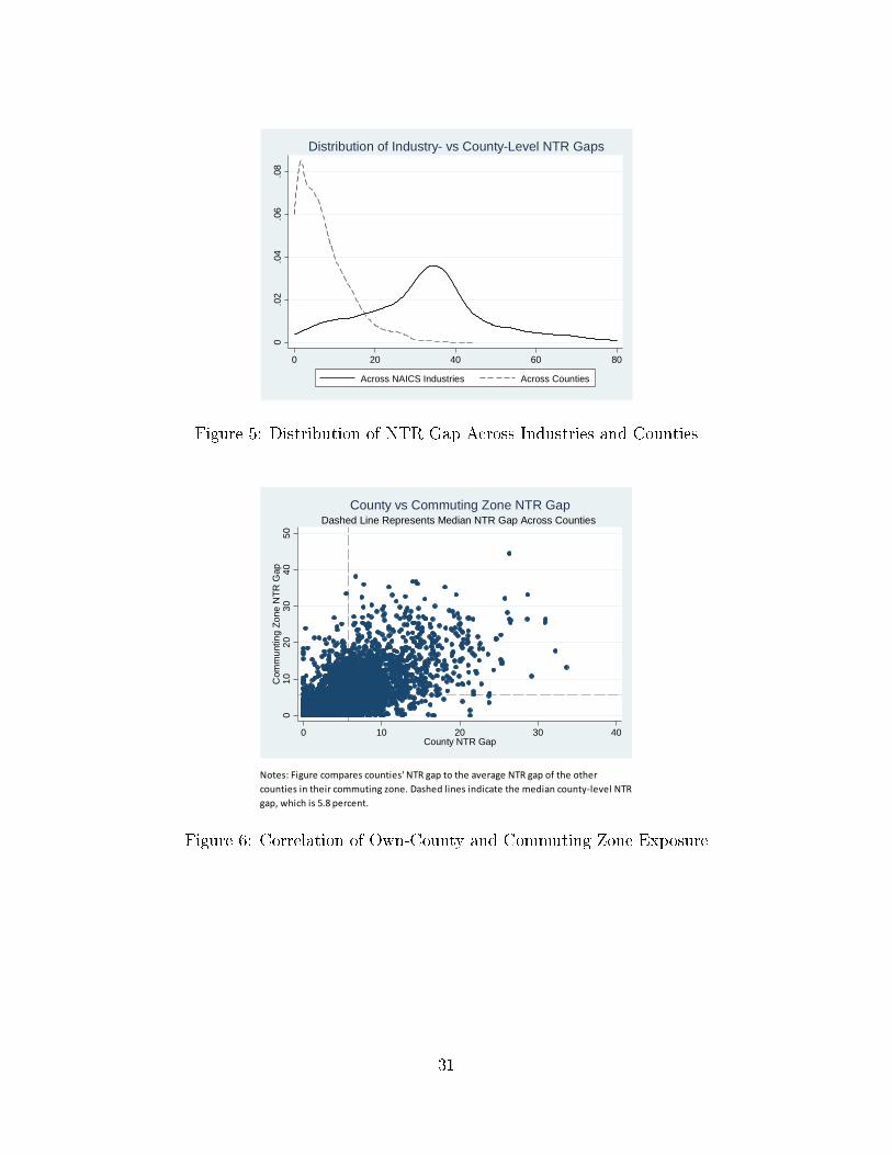
0.0

2.0

4.0

6.0

8

0 20 40 60 80

Across NAICS Industries Across Counties

Distribution of Industry- vs County-Level NTR Gaps

Figure 5: Distribution of NTR Gap Across Industries and Counties

��

��

�� !�"��

010

2030

4050

Com

mun

ting

Zon

e N

TR

Gap

0 10 20 30 40County NTR Gap

Dashed Line Represents Median NTR Gap Across CountiesCounty vs Commuting Zone NTR Gap

Figure 6: Correlation of Own-County and Commuting Zone Exposure

31

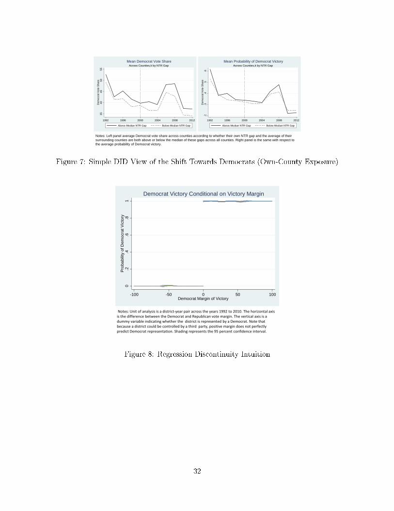
3540

4550

55D

emoc

rat V

ote

Sha

re

1992 1996 2000 2004 2008 2012

Above-Median NTR Gap Below-Median NTR Gap

Across Counties,k by NTR GapMean Democrat Vote Share

.2.3

.4.5

.6D

emoc

rat V

ote

Sha

re

1992 1996 2000 2004 2008 2012

Above-Median NTR Gap Below-Median NTR Gap

Across Counties,k by NTR GapMean Probability of Democrat Victory

Notes: Left panel average Democrat vote share across counties according to whether their own NTR gap and the average of their surrounding counties are both above or below the median of these gaps across all counties. Right panel is the same with respect to the average probability of Democrat victory.

Figure 7: Simple DID View of the Shift Towards Democrats (Own-County Exposure)

��

�� !��"� ��#�� $��#��

�" ��#�� $��

��"��" �� %��#�� $��

�� &��$��'��#� �

0.2

.4.6

.81

Pro

babi

lity

of D

emoc

rat V

icto

ry

-100 -50 0 50 100Democrat Margin of Victory

Democrat Victory Conditional on Victory Margin

Figure 8: Regression Discontinuity Intuition

32

��

�� !�"��

"��#�� $�� %��

&��'��

.3.4

.5.6

.7T

rade

-Rel

ated

Bill

s


Democrat Votes on Trade Bills

Figure 9: Democrats' Votes On Trade Bills

��

�� !��"�#��

��#��$�� !��%�� &��

'��(��

0.2

.4.6

.8E

cono

mic

Ass

ista

nce

Bill

s


Democrat Vote on Economic Assistance Bills

Figure 10: Democrats' Votes On Economic Assistance Bills

33

Appendix

This appendix contains additional empirical results referenced in the main text.

A Legislator Voting Behavior

Figure A.1 displays the McCrary (2008) test of whether there is a discontinuity inthe density of Democrats' winning margin over Republicans. The estimate of thediscontinuity is 0.003 with a standard error of 0.125, indicating that there is not astatistically signi�cant discontinuity. Figures A.2 to A.10 examine the distributionsof each of the district-level attributes included in the legislative voting regressions inSection 5, plotted against the Democrat margin of victory. As discussed there, noneof these distributions exhibit discontinuities at the cuto� point at which the Democratmargin of victory is 0.

B Approaches for Estimating Regression Discontinu-

ity Coe�cient

The nonparametric approach is a �local linear� estimation that uses observations withina window of width w on both sides of the cuto� point and assumes that g(.) and f(.)are linear, with potentially di�erent slopes on the two sides of the cuto� point. Weimplement this approach using the procedure developed by Imbens and Kalyanaraman(2014) to calculate the optimal bandwidth w∗, and estimate analytical standard errorsusing the procedure developed in Porter (2003). In robustness checks, we examinewhether our estimates are sensitive to di�erent bandwidths, e.g., halving and doublingw∗, as in Lee and Lemieux (2010). As indicated in Table A.1, we obtain similar resultsin both cases for both sets of bills.

Parametric estimation, by contrast, uses all of the observations over the domain ofthe assignment variable and assumes high-order polynomial functions of g(.) and f(.).In the main text, we implement this approach using third-order polynomial functionswith potentially di�erent coe�cients on the two sides of the cuto� point. FollowingLee and Card (2008), we calculate standard errors clustered at the assignment variablelevel. Here, we report results using second- and fourth-order polynomials to examinethe sensitivity of our estimates to using third order polynomials. As indicated in TableA.2, we obtain similar results in both cases.

34

Appendix Tables and Figures

��

��

��

��

��

�� ! !

"�#�$%&''� � ( � ��%��)�� ( � ��%��)��

*��$+�$ , � ��- �

&� �� %.�,��/0� 1�� !��2�� 234��3%�

2��.��$�%5 �%(,��

! ��6%.��3�%�0��7��% ,�%��03 �%'%��8�� 4��%3��3%��)��%$�� 0� 4%��)��%

'% ,�%�,��%'%8�� $�%� ��%�%��%��$�� %'�%+,� ,��% ,�%��8�� %��%�%�� %%

�� %��30$�% ,�%$�� 4��%3��3%$��)��8,�%� ��0 ��%��$%��8�� 4��%3��3%

� ��0 ��%$��$%��%(� ��%�%'% ,�% �# �%%&� �� %'�% ,��%�� %��%�088��$�%

234��3%�%��'��% %��30��%'% ,��$%�$��%834��3�%��%�� 0�� 0� %� ��$��$%��%��%

��8� �$%��3+%�''�� %%��%��%��$%��%��)��'4%� � �� 3%��)��'��%� % ,�%��%�%��$%�%8�� %

3��3�

Table A.1: RD Results: Alternate Bandwidths

��

��

��

��

��

�� ! !

"�#�$%&''� � ( � ��%��)�� ( � ��%��)��

*��$+�$ , � ��- �

&� �� %.�,��/0� 1�� !��2�� 234��3%�

2��.��$�%5 �%(,��

! ��6%.��3�%�0��7��% ,�%��03 �%'%��8�� 4��%3��3%��)��%$�� 0� 4%��)��%

'% ,�%�,��%'%8�� $�%� ��%�%��%��$�� %'�%+,� ,��% ,�%��8�� %��%�%�� %%

�� %��30$�% ,�%$�� 4��%3��3%$��)��8,�%� ��0 ��%��$%��8�� 4��%3��3%

� ��0 ��%$��$%��%(� ��%�%'% ,�% �# �%%&� �� %'�% ,��%�� %��%�088��$�%

234��3%�%��'��% %��30��%'% ,��$%�$��%834��3�%��%�� 0�� 0� %� ��$��$%��%��%

��8� �$%��3+%�''�� %%��%��%��$%��%��)��'4%� � �� 3%��)��'��%� % ,�%��%�%��$%�%8�� %

3��3�

Table A.2: RD Results: Alternate Polynomial Functions

35

��

�� !��"��#��$�%��&��#��

�� $�$'��#��!��

�� (��)�$��*�� $+�,$�

0.0

05.0

1.0

15.0

2

-100 0 100Democrat Margin of Victory

McCrary (2008) Manipulation TestDistribution of Democrat Victory Margins

Figure A.1: RD Identifying Assumption Density Test

��

�� !�"��"��

��#�� $�� %�� &��

�'��

13.2

13.2

513

.313

.35

13.4

13.4

5Lo

g P

opul

atio

n


Across Districts, 1992 to 2010Log Population vs Democrat Margin of Victory

Figure A.2: RD Identifying Assumption: Population

36

��

�� !��"��

��#�� !��$�� %�� &��

��'��

910

1112

13Lo

g M

edia

n H

ouse

hold

Inco

me


Across Districts, 1992 to 2010Log Median Household Income vs Democrat Margin of Victory

Figure A.3: RD Identifying Assumption: Household Income

��

�� !��"��

��#�� !��$�� %�� &��

�'��

3.2

3.3

3.4

3.5

3.6

3.7

Log

Per

Cap

ita In

com

e


Across Districts, 1992 to 2010Log Per Capita Income vs Democrat Margin of Victory

Figure A.4: RD Identifying Assumption: Per Capita Income

37

��

�� !"�� #�$�"��%� ��"��

�� "��!��&�� #�$��

'��(��"� �

0.1

.2.3

.4P

erce

nt B

lack

or

Afr

ican

Am

eric

an


Across Districts, 1992 to 2010Percent Black or African American vs Margin of Victory

Figure A.5: RD Identifying Assumption: Black or African American Population Share

��

�� !�"� ��#�$��

��$�� %�� !�"��&�� '��

(��)��

78

910

1112

Per

cent

Bac

helo

rs o

r H

ighe

r


Across Districts, 1992 to 2010Percent Bachelors of Higher vs Democrat Margin of Victory

Figure A.6: RD Identifying Assumption: College or Above Share

38

��

�� !�"��"��

��#�� $�� %�� &��

��'��

810

1214

16P

erce

nt V

eter

an


Across Districts, 1992 to 2010Percent Veteran vs Democrat Margin of Victory

Figure A.7: RD Identifying Assumption: Veteran Share

��

�� !��"��#��

� �!��$�� %�� &��'��

��

.04

.05

.06

.07

.08

Une

mpl

oym

ent R

ate


Across Districts, 1992 to 2010Unemployment Rate vs Democrat Margin of Victory

Figure A.8: RD Identifying Assumption: Unemployment Rate

39

��

�� !�"� ��#�$�� $��

��%�� !�"��&�� '�� (��

��

.09

.095

.1.1

05.1

1P

erce

nt 1

8 or

25


Across Districts, 1992 to 2010Percent 18 to 25 vs Democrat Margin of Victory

Figure A.9: RD Identifying Assumption: 18 to 25 Share

��

�� !�"��#�$��$��

�� %�� !�"��&�� '�� (��

��

.11

.12

.13

.14

.15

Per

cent

65

or O

ver


Across Districts, 1992 to 2010Percent 65 or Over vs Democrat Margin of Victory

Figure A.10: RD Identifying Assumption: Over 65 Share

40

Documents

Does Trade Liberalization with China Influence U.S. Elections? · PDF fileYi Che, Yi Lu, Justin R. Pierce, Peter K. Schott, and Zhigang Tao 2016-039 Please cite this paper as: Che,